Cool Models of Business Cycles

EC6012 2009 Lecture Notes

Stephen Kinsella∗

February 8, 2009

1 Introduction

Economists have been coming up with business cycle models since the timeof Smith, Ricardo, and Marx [5]. Most modern economists take Samuelson’sMultiplier-Accelerator model [12], and Keynes’ model of deficient demandas the starting points for modern policy debates, with the Real BusinessCycle model and it’s ‘computable’ variant, the Dynamic Stochastic Gen-eral Equilibrium model (DSGE), the modern tool for policy evaluation [15].Other business cycle models develop from either behavioural or stock-flowconsistent foundations [7, 1]. We’ll explore one of each in this lecture.

Specifically we’ll look at four models which attempt to generate the cycleswe see in modern economic life. Some of these models are more useful thanothers, some are more used than others. All are cool, for different reasons,hence the title of the lecture. You’ll see why as we go through them.

First, we’ll look at the famous multiplier-accelerator model, then at thefamous predator-prey model of [9, 2], at Minsky’s [10] financial fragilitymodel, and finally at an open economy DSGE model by Obstfeld and Rogoff[11]. We’ll finish off with some numerical examples, and some guides for theproblem set which will get you to read some of the literature around thesemodels.

∗Department of Economics, Kemmy Business School, University of Limerick, Ireland.Email: stephen.kinsella@ul.ie, www.stephenkinsella.net

1

2 Data on Cycles

It is obvious that in 2009 we are living in a downturn of a business cycle—adownturn being a slowing or reversal of the rate of growth of key macroe-conomic indicators, such as GDP, GDP per capita, inventories, gross fixedcapital formation, private investment, a change in the export/import ratio,increases in public sector borrowing requirements, efforts to stimulate ag-gregate demand through expansions of government spending, transfers tobusinesses and private households, and perhaps changes in fiscal and mon-etary policy to accommodate or ameliorate the downturn.

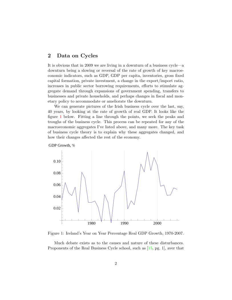
We can generate pictures of the Irish business cycle over the last, say,40 years, by looking at the rate of growth of real GDP. It looks like thefigure 1 below. Fitting a line through the points, we seek the peaks andtroughs of the business cycle. This process can be repeated for any of themacroeconomic aggregates I’ve listed above, and many more. The key taskof business cycle theory is to explain why these aggregates changed, andhow their changes affected the rest of the economy.

1980 1990 2000

0.02

0.04

0.06

0.08

0.10

GDP Growth, %

Figure 1: Ireland’s Year on Year Percentage Real GDP Growth, 1970-2007.

Much debate exists as to the causes and nature of these disturbances.Proponents of the Real Business Cycle school, such as [15, pg. 1], aver that

2

[t]he economy is viewed as being in continuous equilibrium inthe sense that, given the information available, people make de-cisions that appear optimal for them, and so do not make persis-tent mistakes. This is also the sense in which behaviour is said tobe rational. Errors, when the occur, are said to be informationgaps, such as unanticipated shocks to the economy.

This view boils down to a stochastic shock like a pebble being droppedinto the water creates the ripples which we observe as fluctuations in macroe-conomic aggregates like GDP and Unemployment.

Another view, voiced by Hyman Minsky [10] and his followers is financialfluctuations are endogenous to the economy, that, in fact, we create theshocks ourselves through our patterns of behaviour, and the actions of aself-serving government.

Before we start making any judgements, let’s look at cycle data for theIrish economy, from 1970 to the present day.

1980 1990 2000

2 ´ 109

5 ´ 109

1 ´ 1010

2 ´ 1010

5 ´ 1010

Fixed Investment HlogsL

Figure 2: Logged Fixed Investment in Ireland, 1970–2008.

First, let’s look at the multiplier-accelerator model.

3

1980 1990 2000

1 ´ 109

2 ´ 109

5 ´ 109

1 ´ 1010

2 ´ 1010

Government Consumption HlogsL

Figure 3: Logged Government consumption in Ireland, 1970–2008.

1980 1990 2000

2 ´ 107

5 ´ 107

1 ´ 108

2 ´ 108

5 ´ 108

1 ´ 109

Inventory Change HlogsL

Figure 4: Logged changes in inventory for Ireland, 1970–2008. Missing datais a reporting error.

4

1980 1990 2000

1.0 ´ 1010

1.0 ´ 1011

5.0 ´ 1010

2.0 ´ 1010

3.0 ´ 1010

1.5 ´ 1010

7.0 ´ 1010

Total Consumption HlogsL

Figure 5: Logged total consumption in the Irish economy, 1970-2008.

3 Multiplier-Accelerator Models

Simple multiplier accelerator models, which take their intellectual underpin-nings from Samuelson [12], begin from one equation: we have the nationalincome identity

Y = C + I +G+X −M, (1)

which says that national output (Y ) is the sum of Consumption, C, Invest-ment, I, Government expenditure, G, and exports minus imports, X −M .

The question is how do these variables grow, and what causes them tochange in relation to one another?

We have already seen the proxy for changes in Y , or ∂Y/∂t, the changein real GDP over time, in figure 1.

Now, let’s start with the observation that the past is a strong determi-nant of the economy’s performance today. In econo-jargon this means wehave to take account of lagged effects. Looking at a simplified version ofequation 1, and switching off changes in G,X and M for the time being, wehave the lagged dependent relation

Yt = c0 + c1Yt−1. (2)

Equation 2 says that present consumption is a function of past income,

5

and c0,1 as the marginal propensity to consume out of past or present income,respectively. Investment, I, is composed of three parts:

It = I0 + I(r) + b(Ct − Ct−1). (3)

I0 is autonomous investment, that investment which would take placewere there no additional investment in the economy. I(r) is investmentinduced by interest rates. The final part of equation 3 is investment inducedby changes in consumption demand (the ‘acceleration’ principle).

For the model to work, we need b > 0 . We can assume a constantinterest rate pretty easily, which is the same thing as saying let’s drop itentirely. Assuming I(r) = 0 (or alternatively, constant interest), we getthat

It = I0 + b(Ct − Ct−1). (4)

Aggregate demand, when not equal to equilibrium income (and thereforethe macroeconomic accounting identity in equation 2), becomes

Y td = Ct + It = c0 + I0 + cYt−1 + b(Ct − C + t− 1). (5)

If we allow the goods market to be in a rough equilibrium, then Y d = Yat time t, and we have

Yt = c0 + I0 + cYt−1 + b(Ct − Ct−1) (6)

We know the values of Ct and Ct−1 are Ct = c0 + cYt−1, and Ct−1 =c0 + cYt−2 respectively, then substituting these in:

Yt = c0 + I0 + cY t− 1 + b(c0 + cYt−1 − c0 − cYt−2) (7)

We can write equation 7 as a second order linear difference equation, or

Yt − (1 + b)cYt−1 + bcYt−2 = (c0 + I0) (8)

We solve difference equations by finding their equilibrium or steadystates, where Yt = Yt−1 = Yt−2 = Y ∗. Putting this into equation 8 andrearranging, we get

Y ∗ =(c0 + I0)(1− c)

(9)

It is straightforward to perform a stability analysis on this relation, andwe find difference regimes or cycle patterns, depending on the parameter

6

values of b and c chosen for the characteristic function. For details, consult[6, pp. 88-98].

Exercise 1 (Including I(r)) Repeat the analysis above, including a non-zero or non-fixed term for the interest rate’s effect on investment, I(r).What changes are made to the model, and what relevance does an investmentfunction dependent on the interest rate have for modern policy analysis?Think of one real world example where changing the value of r downwardwould either help or hinder investment in the business cycle.

3.1 Lessons & Stylised Facts from Samuelson

The main conclusions from this simple analysis are that, depending on therelationship between the marginal propensity to consume, and the acceler-ation in consumption from year to year. The model does generate cycles,albeit unstable ones. From this simple model we have to take a few lessons:

1. Cycle theory is tricky, and normally requires a bit of differential cal-culus;

2. Some cycles are more ‘cyclical’ than others. Some will explode, somewill dampen, some will oscillate, some will focus in on one point. Thisis where phase plots and arrow diagrams come in really handy;

3. The economy is highly dependent on itself for its current levels ofoutput, employment, etc., so lagged effects are always going to matterin these models.

Finally in this section, let me go through the ‘stylised facts’, NicholasKaldor1 gave in 1958 regarding business cycles.

Kaldor argued these seven facts should form the backdrop for any macroe-conomic theory. In other words, a truly brilliant macroeconomic ‘Theory ofEverything’ should be able to explain and simulate the real world behaviourof these facts. They are

1. Growth at a steady trend rate of aggregate production and labourproductivity;

2. Continued growth of capital per unit of labour1Kaldor, N.Capital Accumulation and Economic Growth in ‘The Theory of Capital’,

F.A. Lutz and D.C. Hague, eds, Macmillan, 1978, pp.178

7

3. A steady state of profit on capital

4. Steady, long period values of capital–output ratios;

5. High correlation between the share of profits in income and the shareof investment in output;

6. Constancy of the functional shares in output in periods when the shareof investment is constant;

7. Wide variation in output growth and growth in labour productivityacross countries.

Exercise 2 (Data Gathering) Using the trading floor or any other datagathering tool, graph the change in any one of Kaldor’s stylised facts for theUS or Irish economies from 1960 to 2008.

3.2 The Non Linear Accelerator

Goodwin [8] showed that by taking account of some limitations of the simpleaccelerator model, it was possible to explain why the capital stock was inshort supply sometimes, and in excess supply at other times, because therelations between the main economic agents are not linear. The model isa simple impulse-response mechanism, and has the very cool property thatinitial conditions (our c0, b0 couplet in the model above) don’t really matterthat much. No matter how the mechanism is started, the system will tendtowards a cycle of some sort.

Goodwin does away with Samuelson’s assumption that the acceleratorneeds realised capital stock to increase in line with output, and posits thatthe rate of investment is limited only by the capacity of the investment goodsindustry. The entrepreneurs in the system have expectations which precludebuilding in a bust, and vice versa. Investment is irreversible, so you can’tunmake a machine or a factory. In an upswing of economic activity theentrepreneurs can’t add capacity fast enough–witness the problems gettingthe WII console to market once demand outstripped supply by orders ofmagnitude—and in the downswing, capital stock can’t be run down fastenough to become competitive overnight, so we end up with excess capacityand unused machines and factories.

3.2.1 The Non Linear Accelerator Model

Call capital stock k, ψ is the desired capital stock proportional to income oroutput, C is consumption, y is income, c0, c1 and b are constants. Assum-

8

ing a linear consumption function which relates consumer spending, C, toincome, Y , such as c = c0 + c1Y D, we have

ψ = by, (10)

C = c0 + c1y, (11)

y = C + k, (12)

Here k denotes the time derivative of the capital stock, which is a proxyfor investment. If the economy seeks to adjust itself perfectly to cycles, thenwe have an overlapping cycle, where either capital is being built too quickly,or being scrapped too slowly, depending on where we are in the businesscycle. When we’re in a boom, producing at capacity, let’s call that buildupof capital k∗. When we’re in a bust, as now, call the scrapping rate k∗∗.We can point to three regimes now, where what k is doing in the economyis very different. Adding them all up, we get a piecewise-linear investmentfunction of the form

k =

k∗, ψ > k,0, ψ = k,k∗∗, ψ < k.

(13)

Now combine equations 10, 11, 12 and 13, to obtain

ψ =b

1− c1k +

c0b

1− c1. (14)

Equation 14, when plotted in phase space for values of k0, k∗, and k∗∗,

shows us a nonlinear system where the equilibrium point is actually unstable,so the system is constantly cycling between extremes of capital extensionor scrappage. The other nice thing about this model is the rate of changeoutside of the equilibrium position. Add any tiny amount of capital to k0,such as k0 + ∆k, and we have a sudden jump to a point like A in the figure.The system then travels slowly down to B, and jumps again very quickly,for opposite reasons. The rectangle ABCD is the limit cycle of this model.

Even though it is really simple, this model is cool for at least four reasons.

1. The final result is independent of initial conditions;

2. The oscillation maintains itself without any stochastic shocks whatso-ever;

3. The equilibrium exists, is attainable, but is unstable, which makessense to us intuitively;

9

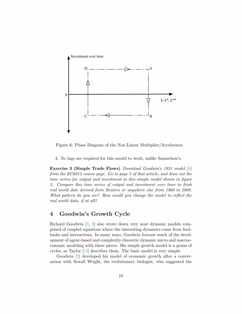
Investment over time

k, k*, k**0

A

BC

D

Figure 6: Phase Diagram of the Non Linear Multiplier/Accelerator.

4. No lags are required for this model to work, unlike Samuelson’s.

Exercise 3 (Simple Trade Flows) Download Goodwin’s 1951 model [8]from the EC6012 course page. Go to page 5 of that article, and draw out thetime series for output and investment in this simple model shown in figure2. Compare this time series of output and investment over time to Irishreal world date derived from Reuters or anywhere else from 1960 to 2008.What pattern do you see? How would you change the model to reflect thereal world data, if at all?

4 Goodwin’s Growth Cycle

Richard Goodwin [8, 9] also wrote down very neat dynamic models com-prised of coupled equations where the interesting dynamics came from feed-backs and interactions. In many ways, Goodwin foresaw much of the devel-opment of agent-based and complexity-theoretic dynamic micro and macroe-conomic modeling with these pieces. His simple growth model is a genus ofcycles, as Taylor [13] describes them. The basic model is very simple.

Goodwin [9] developed his model of economic growth after a conver-sation with Sewall Wright, the evolutionary biologist, who suggested the

10

Lotka-Volterra model of predator-prey interaction from mathematical bi-ology would be apt as both a metaphor and method of analysis for thedynamics of a capitalist macroeconomy. Goodwin took the suggestion andmodelled capitalist-worker dynamics in the following way.

Assume two homogeneous, non-specific factors of production, labour,L and capital, K, where all quantities are real and net, and all wages areconsumed with all profits being reinvested into the system. There is a steadygrowth rate β of the labour force N according to N = N0e

βt, and steadytechnical progress, α so that the capital-labour ratio evolves according toy/l = α = α0e

αt. The capital-output ratio k = Y/L is assumed constant andthe real wage rises in the neighbourhood of full employment. The workersaccrue to themselves a portion of the output of the economy, u and thecapitalists receive v for their efforts.

From these assumptions, and following [6, pgs.449–467], we can derivethe familiar and famous Goodwin equations, where γ andρ are scalars:

v ={[

1k− (α+ β)

]− 1ku

}v (15)

u = − [(α+ γ) + ρv]u (16)

Goodwin, quoted in [6, pgs.57-58], best describes the dynamics of thissystem of equations and their economic meaning:

When profit is greatest, u = u, employment is average,. . . , andthe high growth rate pushes employment to its maximum v2,which squeezes the profit rate to its average value. . . the decel-eration in the growth employment (relative) to its average valueagain, where profit and growth are again at their nadir u2. Thislow growth rate leads to a fall in output and employment to wellbelow full employment, thus restoring profitability to its aver-age value because productivity is now rising faster than wagerates . . . . The improved profitability carries the seed of its owndestruction by engendering a too vigorous expansion of outputand employment, thus destroying the reserve army of labour andstrengthening labour’s bargaining power.

What does this expansion and contraction of the economy look like?The cyclical behaviour of flow of the productive resources from the cap-

italists to the workers and back again can be seen in a different plot, figure4, below

11

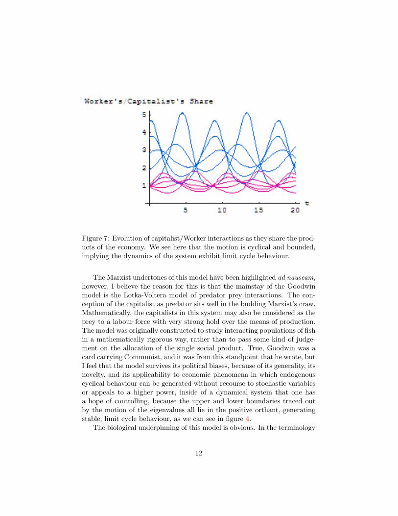
Figure 7: Evolution of capitalist/Worker interactions as they share the prod-ucts of the economy. We see here that the motion is cyclical and bounded,implying the dynamics of the system exhibit limit cycle behaviour.

The Marxist undertones of this model have been highlighted ad nauseam,however, I believe the reason for this is that the mainstay of the Goodwinmodel is the Lotka-Voltera model of predator prey interactions. The con-ception of the capitalist as predator sits well in the budding Marxist’s craw.Mathematically, the capitalists in this system may also be considered as theprey to a labour force with very strong hold over the means of production.The model was originally constructed to study interacting populations of fishin a mathematically rigorous way, rather than to pass some kind of judge-ment on the allocation of the single social product. True, Goodwin was acard carrying Communist, and it was from this standpoint that he wrote, butI feel that the model survives its political biases, because of its generality, itsnovelty, and its applicability to economic phenomena in which endogenouscyclical behaviour can be generated without recourse to stochastic variablesor appeals to a higher power, inside of a dynamical system that one hasa hope of controlling, because the upper and lower boundaries traced outby the motion of the eigenvalues all lie in the positive orthant, generatingstable, limit cycle behaviour, as we can see in figure 4.

The biological underpinning of this model is obvious. In the terminology

12

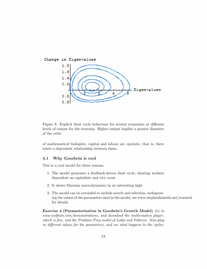
Figure 8: Explicit limit cycle behaviour for several economies at differentlevels of output for the economy. Higher output implies a greater diameterof the orbit.

of mathematical biologists, capital and labour are epistatic, that is, thereexists a dependent relationship between them.

4.1 Why Goodwin is cool

This is a cool model for three reasons.

1. The model generates a feedback-driven limit cycle, showing workersdependent on capitalists and vice versa

2. It shows Marxian macrodynamics in an interesting light

3. The model can be extended to include search and selection, endogenis-ing the values of the parameters used in the model, see www.stephenkinsella.net/researchfor details.

Exercise 4 (Parameterisation in Goodwin’s Growth Model) Go towww.wolfram.com/demonstrations, and download the mathematica player,which is free, and the Predator-Prey model of Lotka and Volterra. Now plugin different values for the parameters, and see what happens to the cycles.

13

Are they stable? Will any parameter value give you the cycle shown in thefigures above? Why, or why not?

5 Minsky’s Model of Financial Fragility

Minsky [10] wrote down several models which purported to show how thedebt structure of large firms and the institutional details of governmentbodies and corporate entities actually led to booms and busts in the financialmarkets, which spilled over into the real economy all too frequently.

Minsky felt that the market was naturally unstable, and the appearanceof stability post-1945 was actually due to the presence of big government,which damped market forces, and the big bank, in the presence of the Fed-eral Reserve and the ECB, etc, large systemically important lenders of lastresort. These were important because, each time the market got itself intotrouble through over lending and was poised for a crash, the combination ofbudget deficits and lender of last resort intervention by the big banks andbig government combined to stabilise aggregate demand in the economy,which allowed asset and income flows, and asset prices and profit flows tobe maintained, until the economy recovered.

In Minsky’s model, booms and busts are the inevitable result of institutionally-legitimised high risk lending practices which, when they go wrong, cost thetax payer billions. Modern speculative finance, Minsky argues, contributesgreatly to the problem by allowing the creation of ever more complex finan-cial products which exploit exotic risk/return profiles in markets which arenot well understood.

Minsky began looking at the data first. Writing in 1985, he documentedthree periods of financial instability between 1945 and 1980, and attemptedto find commonalities between these episodes. These were

1. The deep recession of 1975 in the US;

2. The recession of 1982 in the US;

3. The entire period from 1945–1986 in overview.

Minsky looked at how investment was financed in the modern economyto figure out where the roots of financial instability lay. The fundamentalpropositions of his instability thesis are

1. Capitalist market mechanisms cannot lead to sustained, stable, fullemployment equilibrium;

14

2. Serious business cycles are due to financial attributes that are essentialto capitalism.

I’ll show later just how diametrically opposed to mainstream views Min-sky’s thesis really is. The instability thesis needs to take as given the mannerin which ownership or operating control of assets is financed, in the contextof the institutions which facilitate the transfer of credit from one side of themarket to the other.

By capitalism, Minsky means a system of production and consumptionwhere the means of production are privately owned: the difference betweentotal revenues and labour costs gives income to the owners of the assets, andthose assets can be traded, and the surplus derived from them reinvested inthe system as necessary.

Minskey highlights the role feedbacks play in the generations of boomsand busts very clearly, writing on page 199 of [10]:

The financing of investment by means of new techniques meansthe generation of demand in excess of that allowed for by theexisting tranquil state. The rise in spending upon investmentleads to an increase in profits, which feeds back and raises theprice of capital assets and thus the demand price of investment.Thus, any full-employment equilibrium leads to an expansion ofdebt-financing—weak at first because of the memory of precedingfinancial difficulties—that moves the economy to expand beyondfull employment. Full employment is a transitory state becausespeculation upon and experimentation with liability structuresand novel financial assets will lead the economy to an investmentboom. An investment boom leads to inflation, and, by processesstill to be described, an inflationary boom leads to a financialstructure that is conducive to financial crises.

Minsky highlights the differential effects of expectations on the price ofcapital, depending on the different environments the macroeconomy findsitself in. The price, Pk, of a capital asset is said to be the stream of cashflows one can expect to derive from it (the yield of the asset), and it’sliquidity, which requires that money be in evidence in the system to allowconversion of the asset into money when the owner wants. The functionalrelationship between the price of the asset and the amount of money, M ,in the system depends crucially on the type of expectations assets holdershave at particular times in the business cycle.

15

5.1 Investment

Investment begins with the choice which price to place upon a capital asset.The quantity of money in the system, the value economic agents place onliquidity, and the income and liquidity characteristics embodied by differentcapital assets at different times give us a vector of prices for capital assets,evaluated at a certain point in time.

If we have a market price for a product (and this might not always bethe case—look at the demand for housing in Ireland now), then we can talksensibly about the source of finance for those assets.

The decision to invest is always made in a climate of uncertainty. Howthe potential investor perceives that uncertainty changes over the course ofthe business cycle. The use of finance necessitates the inclusion of time asa realistic modeling problem. Uncertainty differs from risk in that it cannotbe measured by repeated observation, thus one cannot insure against iteffectively. The appropriate liability structure for a capital asset cannot beknown in advance, exacerbating the problem the investor and their bankersface.

5.2 A digression on Money

It should not surprise this class to learn that money is non neutral, that itsvalue is anchored in money wages, and variations in its quantity affect notonly prices, but interest rates also. The central idea of liquidity preference,where the interest rate is determined by the the supply and demand formoney as an asset, has a crucial role to play in understanding where theinternational economy is now. The government can, through a monetaryauthority, affect the interest rate, which will have consequences for outputand employment in an IS-LM world.

The liquidity preference theory is not complete, nor is it a really accuratedescription of what goes on in the economy, because ‘transactions demand’can’t really be described by one mathematical object: one needs two, atleast. One needs to describe how money grows with respect to balancesalready held, and then one needs to describe how these features interact.

6 Minsky, Finally

This treatment follows [14] in its algebraic exposition. This is for two rea-sons. First, the main elements of Minsky’s theory are spread loosely through-out his seminal 1986 book [10], and second, we want to keep the expositional

16

level fairly constant across the models we show today.We start with production. There is a constant markup τ over the wage

bill w, and the labour/output ratio is b. The price level P is determined by

P = (1 + τ)wb. (17)

The profit rate, r, is given by adding up the contributions to profit fromthe various sectors of the economy:

r =PX − wbX

PK=

τwbX

(1 + τ)wbX=

τ

1 + τ

X

K, (18)

HereX is the level of output, K is the capital stock. The core of Minsky’stheory revolves around how expected returns to this capital stock, K. Wehave to have some way of understanding these expectations, and so assumefirms have a rule of thumb when it comes to pricing investments: the price ofcapital should be the sum of anticipated profits, appropriately discounted.There should also be a difference between the current interest rate, and theanticipated return to holding capital.

The investment decision is now a mechanical rule of the form

Pk = (r + ρ)P/i, (19)

here, i is the current interest rate and ρ reflects the difference between theanticipated return to holding capital, and the current profit rate r. ρ hasto carry us a long way in this model, because it represents expected lowor high profits, and is in some sense an index of investor confidence. Theinvestment demand function represents different things at different times inthe cycle. Investment depends on the price differential between capital andthe supply price of new goods, Pi, which we’ll set equal to the regular pricelevel, to give

Pk − P = (r + ρ− i)P/i. (20)

In nominal terms, equation 20 becomes

Investment Demand = PI = [g0 + h(r + ρ− i)]PK. (21)

g0 represents autonomous capital stock growth, h is a coefficient mea-suring firm’s reponsiveness to changes in the price difference between profitand interest costs. If all wages wbX are consumed, and profits rPK aredistributed, we have a savings rate, s. The supply of saving is given by

Saving Supply = srPK = sτwbX. (22)

17

There is a nice interpretation to the equation above: it gives us excessdemand when we take equation 21 from equation 22. Do that, and dividethrough by PK to get the equilibrium condition for the commodity market:

g0 + h(r + ρ− i)− sr = 0. (23)

If the profit rate r or the output level X rises when there is excessdemand, the market will be stable in its adjustment if s − h > 0, in otherwords, investment should respond less than saving to profit rate increases.Solve equation 23 for r, plug it into the investment demand function, andwe get an expression for the capital stock growth rate, g(= I/K).

g = = s[g0 + h(ρ− i)]s− h. (24)

Equation 24 is very cool: a fall in the interest rate, or an increase inanticipated profits leads to higher growth, since

g = sr, (25)

from the saving function, so the profit rate and capacity utilization go upas well.

Now let’s look at the financial side of the economy. Can you see theparallels with the IS-LM approach we used last week?

There is an outside primary asset, F , which we’ll call fiscal debt. Theasset can be converted into money, M , or short term bonds B, and thisbond is held by rentiers. The value of all plant and equipment is PkK =(r + ρ)PK/i. Firms have equity, E, which has a market price at Pe. Thedifference between capital stock and equity is firms’ net worth, N .

We can write the differential of the firms’ balance sheets as

PkI + Pk = PkK = PeE + PeE + N . (26)

We’ll be very interested in seeing how this equation evolves over time.The total wealth of all rentiers is

W = PeE +M +B = PeE + F. (27)

The rentiers’ wealth changes over time according to

W = PeE + PeE + M + B = PeE + srPK. (28)

Rentiers get rich from increases in capital gains and financial saving. Ateach point in time, rentiers have to decide to allocate their wealth acrossassets according to these balancing rules:

18

µ(i, r + ρ)W = M = 0, (29)

ε(i, r + ρ)Pe

W − E = 0, (30)

− β(i, r + ρ)W +B = 0. (31)

Here µ+ ε+ β = 1. The asset demand equations given above determine theinterest rate and the anticipated rate of profit on physical capital, r + ρ.

We can think of r+ρ as representing returns to equity, as wealthy peoplelook for ‘fundamentals’ on the production side of the economy, rather thanpurchasing shares on the Dow Jones average, Pe.

6.1 Digression: Minksy Bubbles

We can alter this model to generate bubbles, by replacing r + ρ in thepreceding equations with an expectations-driven argument. Let the returnto equity be

Πe + (r + ρ)P/Pe, (32)

now, with the actual and expected returns to inflation of equity prices equal,equation 32 can generate a bubble easily. Back to the regular model.

Higher returns will bid up the value of firm’s capital stock in this econ-omy. The same effect happens to their wealth. Combining 27 and 30, wehave

W =F

1− ε(i, r + ρ). (33)

Equation 33 says that increasing r or ρ will drive up ε, and so share pricesand financial prices will rise. Rentier’s net worth is determined macroeco-nomically by their valuation of anticipated profits, which feeds demand forasset supplies and demands in the current period. The share price can besolved for to yield

Pe = (ε/(1− ε))(F/E); (34)

In turn Pe will determine the changes in firms’ net worth, given theirinvestment levels and issuance of new equity, and excess demand in themoney markets will be the sum of

µ(i, r + ρ) =M

F[1− ε(i, r + ρ)], (35)

19

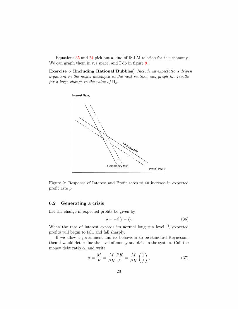
Equations 35 and 24 pick out a kind of IS-LM relation for this economy.We can graph them in r, i space, and I do in figure 9.

Exercise 5 (Including Rational Bubbles) Include an expectations drivenargument in the model developed in the next section, and graph the resultsfor a large change in the value of Πe.

Financial Mkt

Commodity Mkt

Interest Rate, i

Profit Rate, r

Figure 9: Response of Interest and Profit rates to an increase in expectedprofit rate ρ.

6.2 Generating a crisis

Let the change in expected profits be given by

ρ = −β(i− i). (36)

When the rate of interest exceeds its normal long run level, i, expectedprofits will begin to fall, and fall sharply.

If we allow a government and its behaviour to be standard Keynesian,then it would determine the level of money and debt in the system. Call themoney debt ratio α, and write

α =M

F=

M

PK

PK

F=

M

PK

(1f

), (37)

20

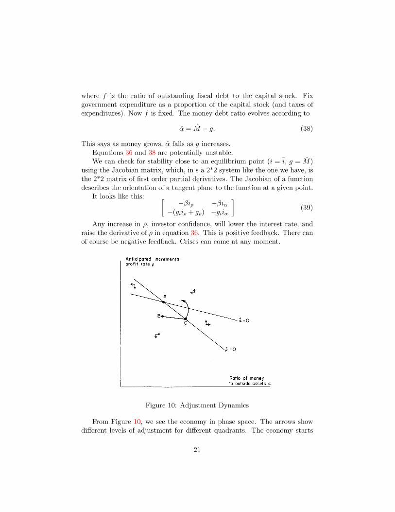
where f is the ratio of outstanding fiscal debt to the capital stock. Fixgovernment expenditure as a proportion of the capital stock (and taxes ofexpenditures). Now f is fixed. The money debt ratio evolves according to

α = M − g. (38)

This says as money grows, α falls as g increases.Equations 36 and 38 are potentially unstable.We can check for stability close to an equilibrium point (i = i, g = M)

using the Jacobian matrix, which, in s a 2*2 system like the one we have, isthe 2*2 matrix of first order partial derivatives. The Jacobian of a functiondescribes the orientation of a tangent plane to the function at a given point.

It looks like this: [−βiρ −βiα

−(giiρ + gρ) −giiα

](39)

Any increase in ρ, investor confidence, will lower the interest rate, andraise the derivative of ρ in equation 36. This is positive feedback. There canof course be negative feedback. Crises can come at any moment.

A MINSKY CRISIS 881

Anticipated incremental

profit rate p

a =o

Ratio of money to outside assets a

FIGURE II

Adjustment Dynamics When a Fall in the Expected Incremental Profit Rate p from an Initial Equilibrium at A Leads Finally to a Return to Steady State

where the subscripts on i stand for derivatives through the

IS/LM system, (7) and (18), and the growth rate derivatives come

from (8). Equations (20) and (21) are potentially unstable. From Figure

I, an increase in p lowers the interest rate and thus raises the

derivative p in (20). This positive feedback does not necessarily

dominate the system, since the Jacobian determinant - i,,figp is

easily seen to be positive (signaling possible stability).

The phase diagram appears in Figure II, with arrows showing

directions of adjustment in the different quadrants. To explore

the possibilities, assume that the economy is initially in a com-

plete steady state equilibrium at point A. A momentary lapse of

confidence would cause p to jump down from A to a point like B.

Equally, a one-shot market operation to reduce the money supply

would cause i to rise. For a newly set (lower) value of a-, (20) shows

that p would start to fall from A, setting off a dynamic process

like the one beginning to B.

If the authorities hold to a constant money supply growth

M when the economy is away from steady state, then a below-

equilibrium value of p is associated with slow capital stock growth

and a rising money-debt ratio a from (21). This increase would

Figure 10: Adjustment Dynamics

From Figure 10, we see the economy in phase space. The arrows showdifferent levels of adjustment for different quadrants. The economy starts

21

at point A. Any drop in investor confidence will move it to point B, whereauthorities will try, through policy, to increase M and hence the money debtratio, α. This would move the economy to point C, and back to equilibrium.If the economy does not turn the corner at C, then the economy enters adebt-deflation scenario, where, quoting Minsky:

Whenever profits decreased hedge units became speculative andspeculative units became Ponzi. Such induced transformations ofthe financial structure lead to falls in the price of capital assetsand therefore to a decline in investment. A recursive processis readily triggered in which a market failure leads to a fall ininvestment which leads to a fall in profits which leads to financialfailures, further declines in investment, profits, additional failure,etc.

7 The Open Economy DSGE Daddy

Obstfeld and Rogoff [11] wrote down a complicated model to do a simplething: unify the new-Keynesian macroeconomics of sticky prices and mo-nopolistic competition with a properly micro founded macrodynamic modelwhich can be modeled using dynamic optimisation techniques. This modelhas started an entire literature extending, developing, and estimating it, soit makes a lot of sense to review it here, as a way of moving us into the nextlecture.

7.1 Setup

There is a continuum of individuals, each of which tries to consume as muchas they can of the single consumption good, z. Consumption of z is indexedby

C =[∫ 1

0c(z)(θ−1)/θdx

](40)

The law of one price holds in this economy, so p(z) = Ep∗(z). The con-sumption based money price index for the economy is

P ={∫ 1

0p(z)1−θ +

∫ 1

0[Ep∗(z)]1−θdz

}1/(1−θ)

(41)

22

If rt is the real interest rate at time t earned on bonds. Ft is the stockof bonds, Mt the stock of money in the economy. The budget constraint isgiven by

PtFt +Mt = Pt(1 + rt−1)Ft−1 +Mt−1 + pt(z)yt(z)− PtCt − PtTt, (42)

where y(z) is the individual’s output and T denotes real taxes paid to thedomestic government. A home resident z maximises a utility function thatdepends positively on consumption and real balances and negatively on workeffort, which is positively related to output:

Ut =∞∑s=t

βs−t

[logCs +

χ

1− ε

(Ms

Ps

)(

1− ε)− κ

2ys(z)2

](43)

Given the utility function, a home individual’s demand for the productz in period t is

ct(z) =[pt(z)Pt

]−θ

Ct (44)

θ is the elasticity of demand with respect to price. Everyone has the samedemand function. The government spends G per period, a sum of

Gt = Tt +Mt −Mt−1

Pt, (45)

Governments take producer prices as given, and, together with private con-sumption, the world demand curve is given by

ydt (z) =

[pt(z)Pt

]−θ

(CWt +GW

t ), (46)

where CWt = nCt + (1− n)Ct is world private consumption demand, which

producers take as given, and government demand is GWt = nGt +(1−n)Gt.

Each individual producer has a degree of monopoly power, giving downwarddemand for its output.

The interest rate parity condition will be

1 + it =Et+1

Et(1 + i∗t ). (47)

The first order conditions for the maximisation problems of home andforeign individuals are

23

Ct+1 = β(1 + rt)Ct, (48)

C∗t+1 = β(1 + rt)C∗t , (49)

Mt

Pt=

[χCt

1 + itit

]1/ε

, (50)

M∗t

P ∗t=

[χC∗t

1 + itit

]1/ε

, (51)

yt(z)(θ + 1)/θ =θ − 1θκ

C−1t (CW

t +GWt )1/θ, (52)

y∗t (z)(θ + 1)/θ =

θ − 1θκ

C∗−1t (CW

t +GWt )1/θ, (53)

Exercise 6 (Pencil and Paper stuff) Go to the website and downloadthe Obstfeld and Rogoff paper. Explain the model to yourself using pencil andpaper, and write down whether the classical Ricardian equivalence postulatewill hold in this world, and why.

These first order conditions do several things. First, the consumptionequations are Euler-formed, which allows us to say something about theoptimal consumption path in the economies. Second, the money marketconditions of equations 50 and 51 show us that money demand depends onconsumption, not income. Third, equations 52 and 53 show us the marginalutility of extra revenue generated from an extra produced unit of z is equalto the disutility from producing it.

In the steady state, all exogenous variable are constant. The steady stateworld interest rate r is given by mixing the two Euler equations to get

r =1− ββ

. (54)

Steady state consumption is given by

C = rF +p(h)(y)P

− G. (55)

Also

C∗ = −r(

n

1− n

)F +

p∗(f)y∗

P ∗− G∗. (56)

We can log-linearise around the symmetric steady state to start compar-ing things, for example, the Dornbusch [3], [4] overshooting model. That’sjust what we’ll do in the next lecture.

24

7.2 Numerical Examples

It’s time to see if you understood any of the preceding bits.

Exercise 7 (Multiplier Accelerator example) There is a

References

[1] George A. Akerlof. Behavioral macroeconomics and macroeconomicbehavior. American Economic Review, 92(3):411–433, 2002.

[2] Heegab Choi. Goodwin’s growth cycle and the efficiency wage hypoth-esis. Journal of Economic Behavior and Organization, 27(2):223–35,July 1995.

[3] R. Dornbusch, S. Fisher, and P.A. Samuelson. Comparative advantage,trade, and payments in a ricardian model with a continuum of goods.The American Economic Review, 67(3):823–839, December 1977.

[4] Rudiger Dornbusch. Expectations and exchange rate dynamics. Journalof Political Economy, 84(6):1161–1176, 1976.

[5] Duncan K. Foley. Understanding Capital: Marx’s Economic Theory.Harvard University Press, 1986.

[6] G. Gandolfo. Economic Dynamics: Study Edition. Springer, Amster-dam, 1st edition edition, 2003.

[7] Wynne Godley. Money and credit in a keynesian model of incomedetermination. Cambridge Journal of Economics, 23(2):393–411, April1999.

[8] R. M. Goodwin. The nonlinear accelerator and the persistence of busi-ness cycles. Econometrica, 19:1–17, 1951.

[9] Richard Goodwin. A growth cycle. In C. H. Feinstein, editor, Social-ism, Capitalism, and Growth. Cambridge: Cambridge University Press,1967.

[10] Hyman P. Minsky. Stabilising and Unstable Economy. McGraw-Hill,New York, 1986.

[11] Maurice Obstfeld and Kenneth Rogoff. Exchange rate dynamics redux.Journal of Political Economy, 103(3):624–60, 1995.

25

[12] Paul A. Samuelson. Interaction between the multiplier analysis and theprinciple of acceleration. Review of Economics and Statistics, 21(2):75–78, 1939.

[13] Lance Taylor. Reconstructing Macroeconomics: Structuralist Critiquesof the Mainstream. Harvard University Press: Boston, 2004.

[14] Lance Taylor and Stephen O’Connell. A minsky crisis. Quarterly Jour-nal of Economics, 100(Supplement):871–885, 1985.

[15] Michael Wickens. Macroeconomic Theory. Princeton University Press,Princeton, New Jersey and Oxford, 2008.

26