convexity overview revu merger - Polytech Niceusers.polytech.unice.fr/~hugues/Polytech/IMAFA/Didier...
98
Convexity overview Convexity overview Didier Faivre
Transcript of convexity overview revu merger - Polytech Niceusers.polytech.unice.fr/~hugues/Polytech/IMAFA/Didier...
Convexity overviewConvexity overview
Didier Faivre
2
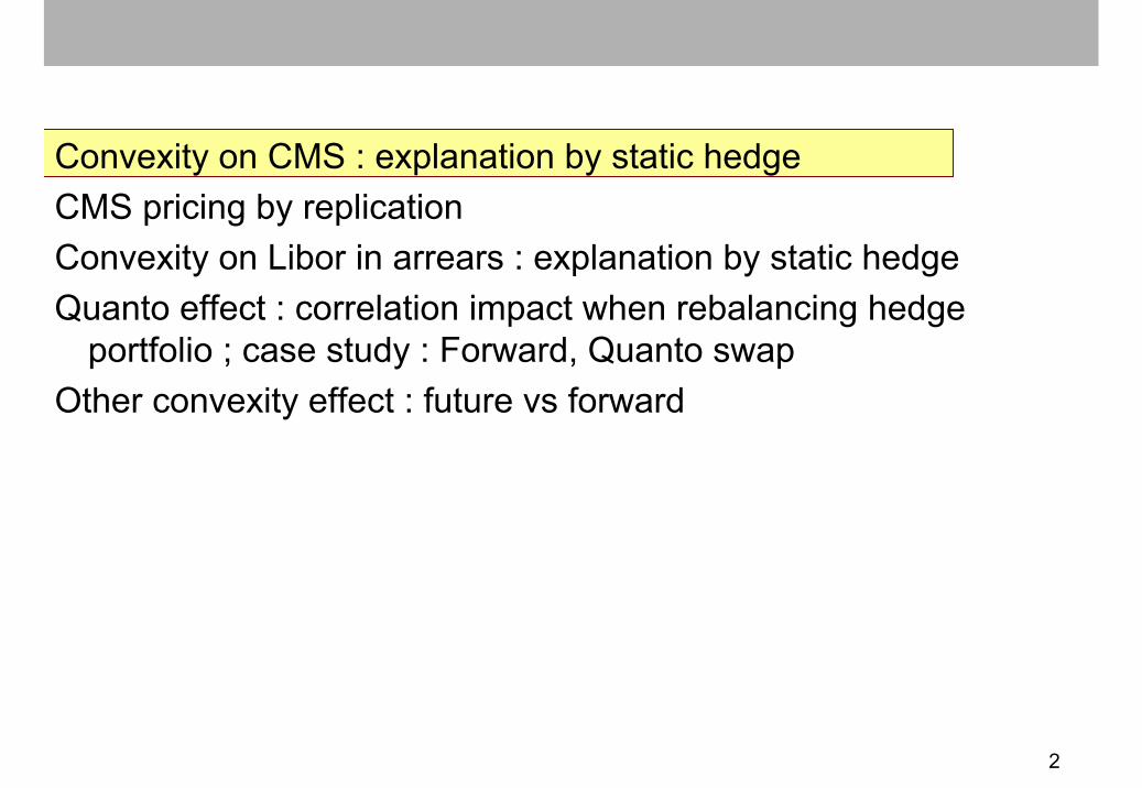
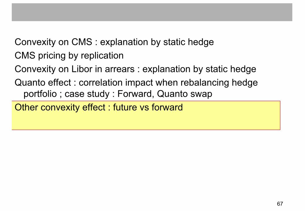
Convexity on CMS : explanation by static hedgeCMS pricing by replicationConvexity on Libor in arrears : explanation by static hedgeQuanto effect : correlation impact when rebalancing hedge
portfolio ; case study : Forward, Quanto swapOther convexity effect : future vs forward
3
topics
The presentation will focus on the Investment Bank risk-management, which is the real life explanation for convexity, not on formula.

4
CMS definition
Reminder : CMS definitionA CMS rate nYears is the rate at which one would exchange at time T’the swap rate of maturity n Years, this swap rate being fixed at time T with :
Pricing at date t of the CMS
nY which will be fixed at Tand paid at date T’ : CMS(t,T,T’)
t
Fixing of the swap rate of maturity nY : S(T,nY)
T T’
CMS(t,T,T’)
S(T,nY) = CMS(T,T,T ’)
Flows exchange
TT ≥'
5
CMS definitionRemarks
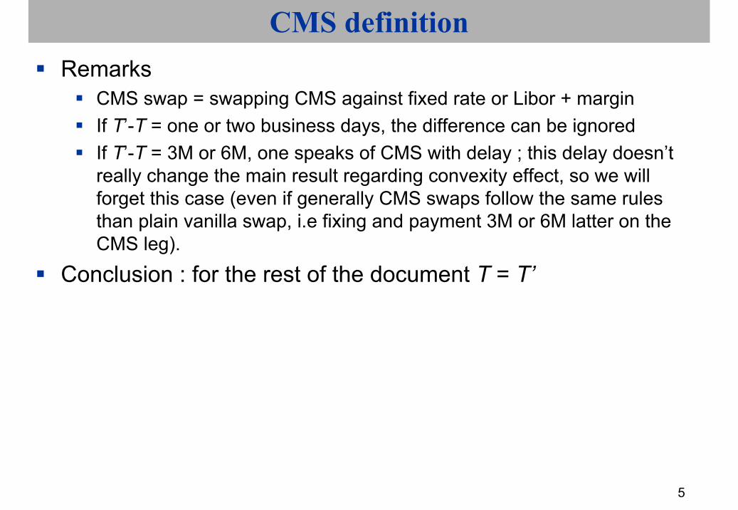
CMS swap = swapping CMS against fixed rate or Libor + marginIf T’-T = one or two business days, the difference can be ignoredIf T’-T = 3M or 6M, one speaks of CMS with delay ; this delay doesn’t really change the main result regarding convexity effect, so we will forget this case (even if generally CMS swaps follow the same rules than plain vanilla swap, i.e fixing and payment 3M or 6M latter on the CMS leg).
Conclusion : for the rest of the document T = T’

6
Examples of the Bank Quotations as of 19/5/2003
10Y swap : CMS10Y-120 against EURIBOR6M10Y swap : CMS10Y-111 against EURIBOR6M without convexity adjustment (vol = 0)
10Y swap : CMS5Y-81 against EURIBOR6M10Y swap : CMS5Y-75 against EURIBOR6M without convexity adjustment (vol = 0)
5Y swap : CMS2Y-43 against EURIBOR6M5Y swap : CMS2Y-41 against EURIBOR6M without convexity adjustment (vol = 0)

7
Examples of the Bank Quotations as of 19/5/2003
swaps forwards and swaps forwards with convexity adjustment : 10 Y vs EURIBOR6M
4.00%
4.20%
4.40%
4.60%
4.80%
5.00%
5.20%
5.40%
5.60%
5.80%
0.5 1.5 2.5 3.5 4.5 5.5 6.5 7.5 8.5 9.5
horizon
rate
s
0.01%
0.03%
0.05%
0.07%
0.09%
0.11%
0.13%
0.15%
fwd fwd with convexity adjustment convexity adjustment

8
Convexity effect on CMS
Start with an example :Quotation, as of 15/5/2003, EUR market, 30/360 fixed rate swap againstLibor 3M :
CMS 10Y in 5Y, paid in 5Y : 5.480%Forward swap 10Y in 5Y : 5.381%In 5Y, the client will receive :
Notional ×(fixing Swap10Y in 5Y-5.48%) ×coverageWe take coverage =1, just for illustration purpose

9
Convexity effect on CMS
Remark :The difference is the same whatever the frequency of the Libor : 3M,
6M, 12M…
How can the difference be explained ?
10
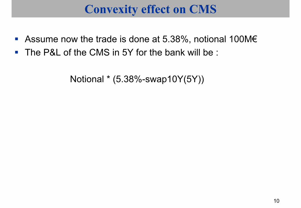
Convexity effect on CMS
Assume now the trade is done at 5.38%, notional 100M€The P&L of the CMS in 5Y for the bank will be :
Notional * (5.38%-swap10Y(5Y))

11
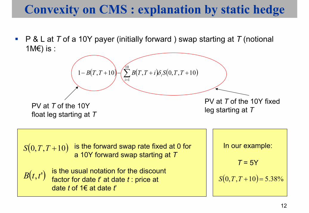
Convexity on CMS : explanation by static hedge
What would be a static hedge ?The only static hedge without options would be sellingforward swapSuppose that we want to hedge the 10Y in 5Y CMS by a payer swap forward 10Y in 5Y, the nominal of a deal being 100M.What would be the notional ?
We start by giving some formulas for valuation of a the P&L of a payer 10Y forward swap
12
Convexity on CMS : explanation by static hedge
P & L at T of a 10Y payer (initially forward ) swap starting at T (notional1M€) is :
( ) ( ) ( ) 10,,0, 10,110
1∑=
++−+−i
i TTSiTTBTTB δ
PV at T of the 10Yfloat leg starting at T
PV at T of the 10Y fixedleg starting at T
( )10,,0 +TTS is the forward swap rate fixed at 0 for a 10Y forward swap starting at T
( )', ttB is the usual notation for the discount factor for date t’ at date t : price atdate t of 1€ at date t’
In our example:
T = 5Y
( ) %38.510,,0 =+TTS

13
Convexity on CMS : explanation by static hedge
Then again, the P & L at T of a 10Y payer swap starting at T is :
( ) ( ) ( ) 0 , 10,110
110 =+−+− ∑
=iYi TSiTTBTTB δ
PV at T of the 10Yfloat leg starting at T PV at T of the 10Y fixed
leg starting at T
( ) ( )10,10 += TTSTS Yis the swap rate fixed at T for a 10Y swap starting at T
We just replaced by ( ) ( )10,10 += TTSTS Y( )10,,0 +TTS

14
Convexity on CMS : explanation by static hedge
Then we get for the P&L of the 10Y payer swap starting at T :
Just for simplification, we set :
( ) ( )( ) ( ) =++−∑=
iTTBTTSTS ii
Y , 10,,0 10
110 δ
( ) ( )( )10,,010 +−× TTSTSical Levelphys Y
1 ii ∀=δ
15
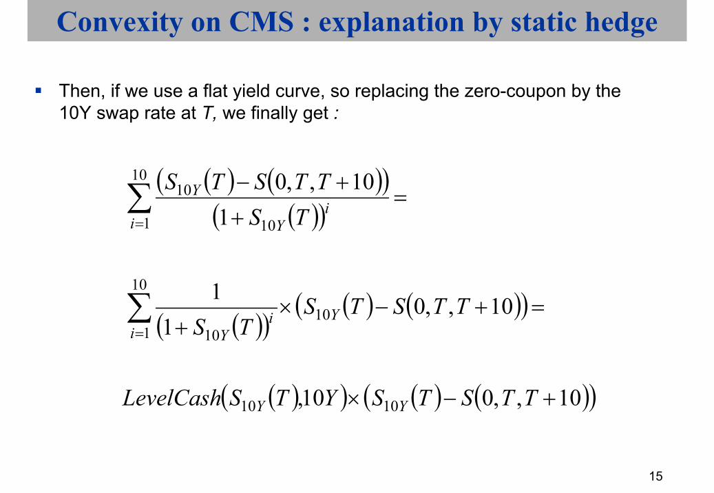
Convexity on CMS : explanation by static hedge
Then, if we use a flat yield curve, so replacing the zero-coupon by the 10Y swap rate at T, we finally get :
( ) ( )( )( )( )
( )( )( ) ( )( )
( )( ) ( ) ( )( )10,,010,
10,,01
1
1
10,,0
1010
10
10
1 10
10
1 10
10
+−×
=+−×+
=+
+−
∑
∑
=
=
TTSTSYTSLevelCash
TTSTSTS
TSTTSTS
YY
Yi
iY
ii
Y
Y

16
Convexity on CMS : explanation by static hedge
In our example, the P&L in 5Y of a10Y payer swap (notional 1M€) starting in 5Y :
We remind that the P&L on the CMS is :
Notional * (5.38% - )
( )( )( )( )%38.5
11
10
10
1 10
−×+
∑=
TSTS Y
ii
Y
( )TS Y10
17
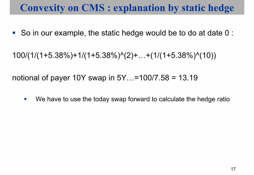
Convexity on CMS : explanation by static hedge
So in our example, the static hedge would be to do at date 0 :
100/(1/(1+5.38%)+1/(1+5.38%)^(2)+…+(1/(1+5.38%)^(10))
notional of payer 10Y swap in 5Y…=100/7.58 = 13.19
We have to use the today swap forward to calculate the hedge ratio
18
Convexity on CMS : explanation by static hedge
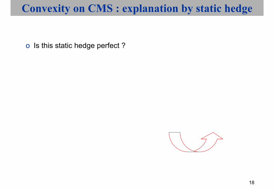
o Is this static hedge perfect ?
Of course not !

19
( ) ( )( )( )( )
( )( )( )( )
( )( )( )( )
( )( )( )( )
+−
+++
−+
+−
++
−×+−× 10
10
103
10
102
10
10
10
1010 1
%38.51
%38.51
%38.51
%38.53.191 )(%38.5100TS
TSTS
TSTS
TSTS
TSTSY
Y
Y
Y
Y
Y
Y
YY L
Convexity on CMS : explanation by static hedgeWhat happens if the bank prices the CMS at the forward swap
rate ?In 5Y the client will receive the fixing of the swap 10Y in 5Y and pay 5.38%The P&L of the Bank in 5Y on the CMS deal is :
P&L swap fwdCMS P&L (Formula of page 15)
P&L Bank = P&L swap fwd + P&L CMS

20
Convexity on CMS : explanation by static hedge
-P&L Bank on a 10Y CMS in 5Y, if pricing of CMS = forward rate and static hedgein M EUR, 100M nominal transaction
0.0
0.2
0.4
0.6
0.8
1.0
1.2
1.4
1.6
1.8
2.0
0.50% 1.00% 1.50% 2.00% 2.50% 3.00% 3.50% 4.00% 4.50% 5.00% 5.50% 6.00% 6.50% 7.00% 7.50% 8.00% 8.50% 9.00% 9.50% 10.00%
10.50%
11.00%
11.50%
12.00%
12.50%
swap10Y (in 5Y)
-P&
L B
ank
21
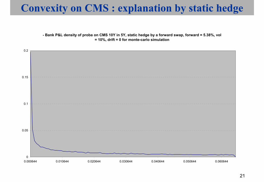
Convexity on CMS : explanation by static hedge
- Bank P&L density of proba on CMS 10Y in 5Y, static hedge by a forward swap, forward = 5.38%, vol = 10%, drift = 0 for monte-carlo simulation
0
0.05
0.1
0.15
0.2
0.000644 0.010644 0.020644 0.030644 0.040644 0.050644 0.060644

22
Convexity on CMS : explanation by static hedge
- Bank P&L density of proba on CMS 10Y in 5Y, static hedge by a forward swap, forward = 5.38%, vol = 10%, drift = 1% for monte-carlo simulation
0
0.01
0.02
0.03
0.04
0.05
0.06
0.00193 0.02193 0.04193 0.06193 0.08193 0.10193

23
Convexity on CMS : explanation by static hedge
Some remarks :Of course the P&L is 0 if swap10Y is 5.38% in 5Y.The first order derivative of the P&L with respect to the swap10Y is 0 at
5.38% value, by definition of the chosen hedge ratio.
P&L of the Bank in function of the swap10Y :As we can see on the graphs page 11 ( –P&L of the Bank as a function of swap10Y ) and page 12 and 13 (distribution of -P&L of bank, from two monte-carlo simulations), this P&L is always negative !It means that a static hedge is not efficient

24
Convexity on CMS : explanation by static hedge
We also see on the graph that –P&L the Bank is a convex function of the swap10Y ; this can also be checked by immediate calculation :
See Annex 1 for some definitions/interpretations of convexity
( )
( ) ( ) ( ) ( ) ( )Swap10Y offunction convex a is
1011
101%38.5
101%38.5
101%38.5
101%38.5
Swap10Y offunction linear a is %38.510
101032 YswapYswapYswapYswapYswap
YSwap
++
+++
++
++
+
−
L

25
Convexity on CMS : explanation by static hedge
Conclusions :The static hedge leads to negative P&L, whatever the swap10Y in 5Y
This means that the Bank has to settle a dynamic hedge; the previous results can also be used to show that any hedge rebalancing (and a fortiori two way ticket due to gamma rebalancing) generate a negative P&L

26
Convexity on CMS : explanation by static hedge
the Bank is gamma negative (we could also say short of volatility) and this must be taken into account in the price made to the client (10bp of “convexity adjustment”).
the hedge in volatility is in practice dynamically done by buying swaptions on 10Y underlying the maturity of which is the horizon of the CMS (5Y in or example), in order to be both delta and gamma neutral hedged : this hedge has a price, and this another interpretation for the additional 10bp of convexity adjustment.

27
Convexity on CMS : explanation by static hedge
Additional Remarks :Of course the previous results are true whatever the CMS underlying swap or the horizon of the CMS
The higher the maturity of the CMS underlying swap, the higher the convexity adjustment

28
Convexity on CMS : explanation by static hedge
The higher the horizon of the CMS, the higher the convexity adjustment
The higher the implied volatility on the CMS underlying swap, the higher the convexity adjustmentWe give in annex 2 an approximate formula to calculate the convexity adjustment using one unique implied volatility (ATM) ; a more acute and complex method use the full smile on the CMS underlying swap
29
Convexity on CMS : explanation by static hedge
Last but not least remark :In the previous pages, we made an approximation to calculate the P&L : the coupon 5.38 was discounted with a unique discount rate, the 10Y swap, not a zero-coupon curve ; using a zero-coupon curve would have given the same results, but with far less easy graphical representation or monte-carlo simulation (of course the P&L remains a convex function of the 10 zero-coupon rates).
30
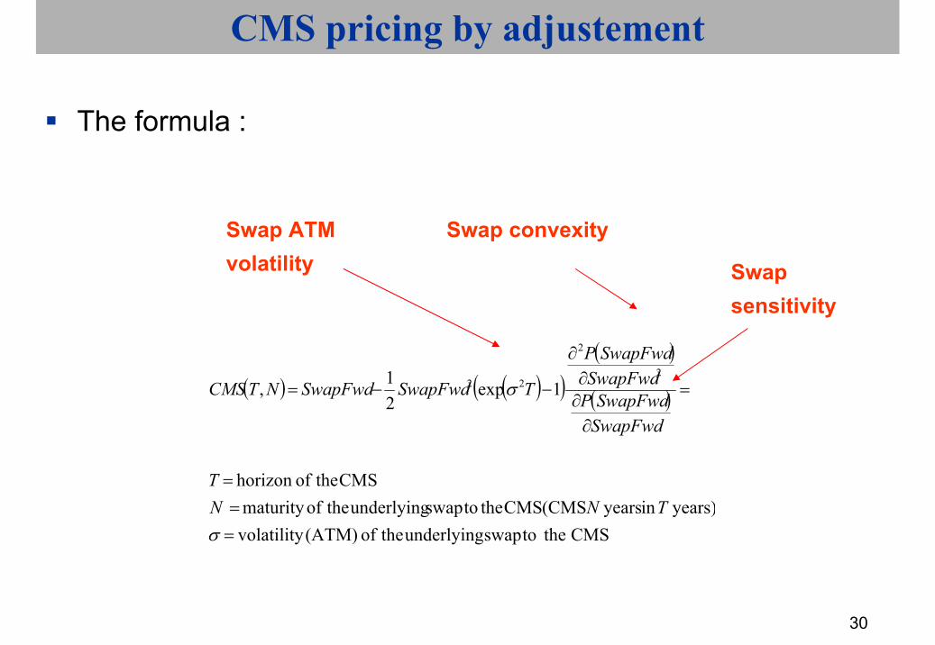
CMS pricing by adjustement
The formula :
( ) ( )( )( )
( )
CMS the toswap underlying theof (ATM) volatilityyears) in years (CMS CMS the toswap underlying theofmaturity
CMS theofhorizon
1exp21,
2
2
22
===
=
∂∂∂
∂
−−=
σ
σ
TNN T
SwapFwdSwapFwdP
SwapFwdSwapFwdP
TSwapFwdSwapFwdNTCMS
Swap convexity
Swap sensitivity
Swap ATM volatility

31
CMS pricing by adjustment
Simplified version of the formula (same result)
( )
( )( )( ) ( )( )
( )( )( ) ( )( )
( )( )( ) ( )( ) adjustmentconvexity called is
11111exp1
20 0.5, a annuel, semi 10Y, : exemplecoupons ofnumber total
leg fixed on the swap theofy 1/frequenc a
11111exp1
11111exp
2
2
2
−++−−+
====
>
−++−−+
−++−−+
=
N
N
N
aSwapFwdaSwapFwdaNSwapFwdT
NN
SwapFWdaSwapFwdaSwapFwd
aNSwapFwdTSwapFwd
aSwapFwdaSwapFwdaNSwapFwdTSwapFwdSwapFwd
T,NCMS
σ
σ
σ

32
A sketch of proof for convexity adjustment
We consider first a bond :with N year maturity at date TWe note r(T) the forward yield at date T, P(T) the forward price at date T.The dynamic of r is (under forward neutral probability) :
(warning : here σ standard deviation, not volatility)The dynamic of P(T) is then (Ito lemma) :
( ) ttt dWdtTdr σ+µ=
( )( ) ( ) ( )( ) ( )( ) tttttt dWTrPdtTrPdtTrPdP ′σ+″σ+′µ= 2
21

33
A sketch of proof for convexity adjustment
The forward price of the bond is by definition a martingale under the forward neutral probability :
This gives formula of previous slide when seeing a swap as a bond and by replacing standard deviation by volatility
( ) ( )( )( )( )
dtTrP
TrPi
ti
iti
iit ′
″σ−=µ 2
21
34
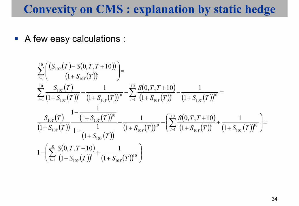
Convexity on CMS : explanation by static hedge
A few easy calculations :
( ) ( )( )( )( )
( )( )( ) ( )( )
( )( )( ) ( )( )
( )( )( )
( )( )
( )( )( )( )
( )( )( ) ( )( )
( )( )( ) ( )( )
++
++
−
=
++
++
−+
+
+−
+−
+
=+
−+
+−
++
+
=
++−
∑
∑
∑ ∑
∑
=
=
= =
=
1010
10
1 10
1010
10
1 1010
10
10
1010
10
10
10
1
10
110
101010
1010
10
10
1 10
10
11
110,,01
11
110,,0
11
111
111
1
11
110,,0
11
1
110,,0
TSTSTTS
TSTSTTS
TSTS
TSTS
TS
TSTSTTS
TSTSTS
TSTTSTS
Yii
Y
Yii
YY
Y
Y
Y
Y
i i Yi
YYi
Y
Y
ii
Y
Y

35
Convexity on CMS : explanation by static hedgeCMS pricing by replicationConvexity on Libor in arrears : explanation by static hedgeQuanto effect : correlation impact when rebalancing hedge
portfolio ; case study : Forward, Quanto swapOther convexity effect : future vs forward
36
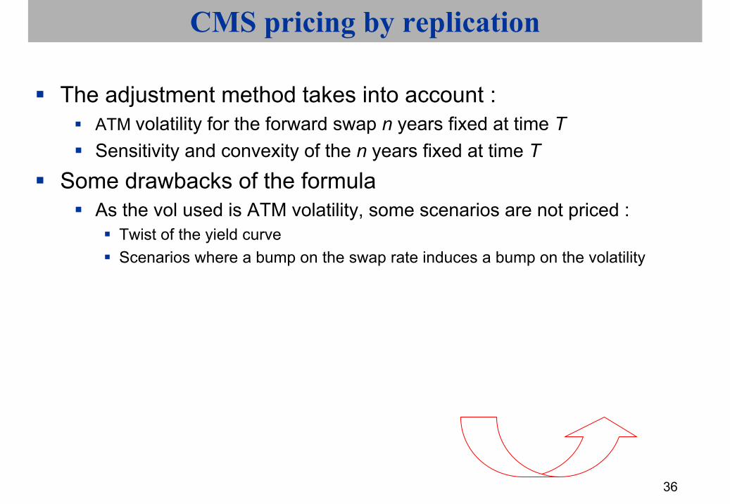
CMS pricing by replication
The adjustment method takes into account :ATM volatility for the forward swap n years fixed at time TSensitivity and convexity of the n years fixed at time T
Some drawbacks of the formulaAs the vol used is ATM volatility, some scenarios are not priced :
Twist of the yield curveScenarios where a bump on the swap rate induces a bump on the volatility

37
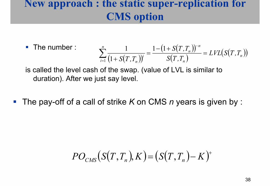
New approach : the static super-replication for CMS option
Reminder 1 :the pay-off of a cash-settled swaptions of strike K on a n years swap is given by :
( )( )( )( )
( ) ( )( )nn
nn
n
ii
n
T,TSLVLT,TS
T,TST,TS
=+−
=+
−
=∑ 11
11
1
( )( )( )( )
( )( )
( )( )( ) ( )( )
( )( ) ( )( )+
+−
+
=
−
=−+−
=−+
=∑
KT,TST,TSLVL
KT,TST,TS
T,TS
KT,TST,TS
K,T,TSPO
nn
nn
nn
n
n
ii
nncw
11
11
1
38
New approach : the static super-replication for CMS option
The number :
is called the level cash of the swap. (value of LVL is similar to duration). After we just say level.
The pay-off of a call of strike K on CMS n years is given by :
( )( ) ( )( )+−= KTTSKTTSPO nnCMS ,,,
( )( )( )( )
( ) ( )( )nn
nn
n
ii
n
T,TSLVLT,TS
T,TST,TS
=+−
=+
−
=∑ 11
11
1
39
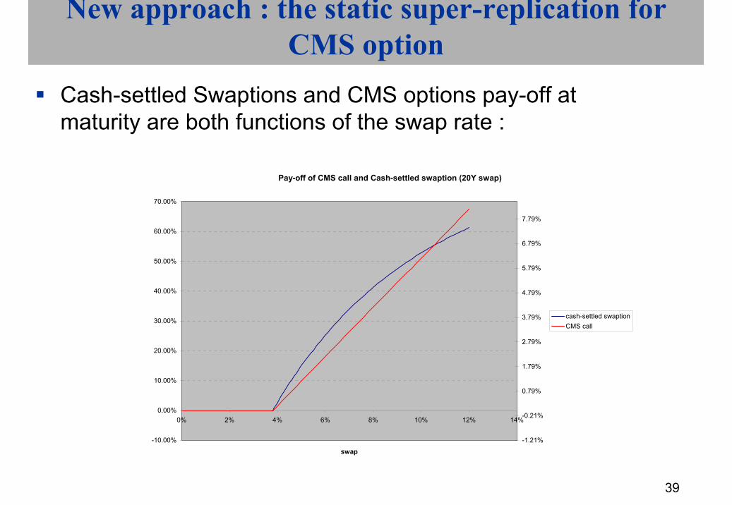
New approach : the static super-replication for CMS option
Cash-settled Swaptions and CMS options pay-off atmaturity are both functions of the swap rate :
Pay-off of CMS call and Cash-settled swaption (20Y swap)
-10.00%
0.00%
10.00%
20.00%
30.00%
40.00%
50.00%
60.00%
70.00%
0% 2% 4% 6% 8% 10% 12% 14%
swap-1.21%
-0.21%
0.79%
1.79%
2.79%
3.79%
4.79%
5.79%
6.79%
7.79%
cash-settled swaptionCMS call
40
New approach : the static super-replication for CMS option
Tricky issue : CMS call is linear function of the swap and swaption is concave in the swap rateAnyway, one can try to replicate the pay-off of the CMS call with a string of cash-settled swaptions with different strikeswith same maturity and underlying swap :
Let’s note
the strikes of the cash-settled swaptions for the super-replication.nKKKK <<<= L21

41
New approach : the static super-replication for CMS option
We want to find the weights such that :
We will choose the weights so that the previous equality between the pay-off of the call on CMS and the weighted sum of cash-settled swaptions is exact each time the swap is equal to one the strikes :
( )nTTS ,
jK
( )( ) ( )( )incw
n
iinCMS KTTSPOwKTTSPO ,,,,
1∑=
≈
( ) ( ) ,,,1
jKKPOwKKPO ijcw
n
iijCMS ∀=∑
=
iw
iw

42
New approach : the static super-replication for CMS option
If , the pay-off of the CMS call is zero, same thing for basket of swaptions.If , we just have to write :
If
KKS == 1
2KS =
( ) ( ) ( ) ( )( )122121
212 ,, KKKLVLwKKPOwKKPOKK icw
n
iiCMS −===− ∑
=
3KS =
( ) ( ) ( )
( )( ) ( )( )23321331
31
313 ,,
KKKLVLwKKKLVLw
KKPOwKKPOKK icw
n
iiCMS
−+−=
==− ∑=

43
New approach : the static super-replication for CMS option
So
By iteration, it can be shown that for I ≥ 3 :
( )( ) ( ) ( )
−
−−
=2323
132
11KLVLKLVLKK
KKw
( ) ( )
( ) 1
11
1
1
11
1
1
1
11
1
1
11
−
−
−
+
−+
−+
−+
+
−−
+
−−
−−
−−
=
ii
i
i
ii
ii
ii
i
iii
i
ii
KKKK
KLVL
KKKK
KKKK
KLVLKKKK
KLVLw
44
New approach : the static super-replication for CMS option
Weights Properties Weights are independent of the level of the swapas well as the smile
The replication is a static oneReplication methodology provides both
Exact pricingHedging
Then, for CMS pricing, just use the call-put parity, hoping you get the same CMS whatever the strike !
(use swap forward as a good choice for strike)

45
New approach : the static super-replication for CMS option : Call CMS

46
New approach : the static super-replication for CMS option
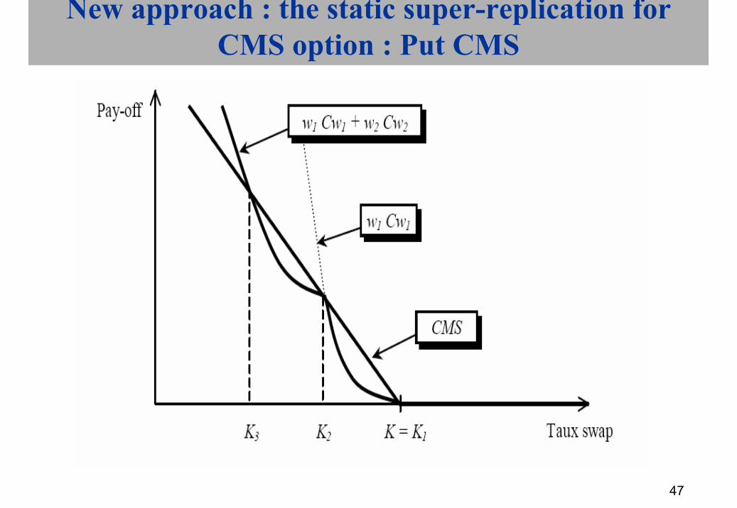
For the put on CMS we find the same formula with decreasing strikes.
Then we have an under-replicationthe first weight is positive and the other negative.
47
New approach : the static super-replication for CMS option : Put CMS

48
New approach : the static super-replication for CMS option : summary

49
New approach : the static super-replication for CMS option
In practice, to begin with replication :To price a Cap, choose a geometric step h, let’s say 10-3Choose and set and so on…To price, a put do the same thingTo price a CMS, price the call and the put of same strike, choosing the forward swap or the CMS with convexity adjustment as a strike
KK =1( )hKK +×= 112

50
New approach : the static super-replication for CMS option
But in fact, it’s more complex :You need a smile modelling and use the following formulas for CMS option of maturity T0 and swap starting at Tf :
51
New approach : the static super-replication for CMS option
You have to define upper and lower bound for integration in the previous formulasAnd also upper and lower bound for your smile modeling (outside the bounds, take constant formulas)Of course
the greater the maturity of the CMS underlying, the greater the maturity of the CMS option or CMS fixing
The greater the sensitivity of the price to the bounds !
52
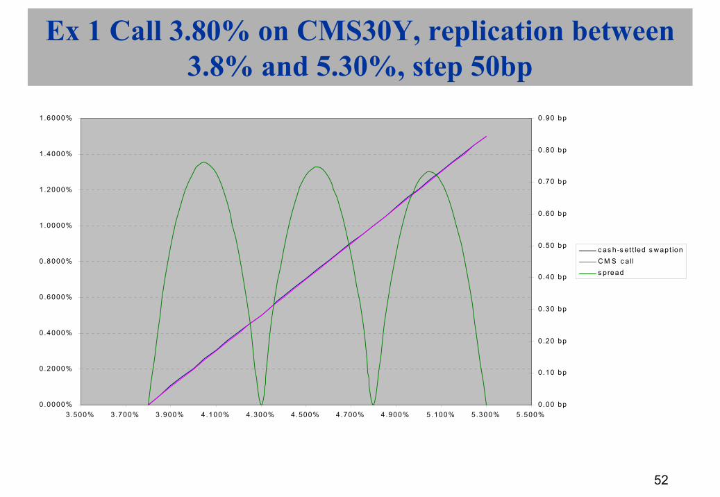
Ex 1 Call 3.80% on CMS30Y, replication between3.8% and 5.30%, step 50bp
0.0000%
0.2000%
0.4000%
0.6000%
0.8000%
1.0000%
1.2000%
1.4000%
1.6000%
3.500% 3.700% 3.900% 4.100% 4.300% 4.500% 4.700% 4.900% 5.100% 5.300% 5.500%0.00 bp
0.10 bp
0.20 bp
0.30 bp
0.40 bp
0.50 bp
0.60 bp
0.70 bp
0.80 bp
0.90 bp
c as h-s e t t led s w apt ionC M S c a lls pread

53
Ex 2 Put 3.80% on CMS30Y, replication between2.3% and 3.80%, step 50bp
0.0000%
0.2000%
0.4000%
0.6000%
0.8000%
1.0000%
1.2000%
1.4000%
1.6000%
2.300% 2.500% 2.700% 2.900% 3.100% 3.300% 3.500% 3.700% 3.900%-0.90 bp
-0 .80 bp
-0 .70 bp
-0 .60 bp
-0 .50 bp
-0 .40 bp
-0 .30 bp
-0 .20 bp
-0 .10 bp
0.00 bp
0.10 bp
c as h-s e t t led s w apt ionC M S puts pread

54
Ex 3 CMS EURO against EURIBOR6M
CMS+ margin against EURIBOR 6Mmargin quotations
10Y CMSreplic adjust difference of margin
5Y -129bp -128bp -0.48bp10Y -96bp -95bp -1.03bp15Y -82bp -80bp -2.17bp20Y -72bp -69bp -2.92bp30Y -64bp -60bp -3.72bp
20Y CMSreplic adjust difference of margin
5Y -163bp -162bp -0.79bp10Y -121bp -118bp -2.57bp15Y -101bp -96bp -4.32bp20Y -88bp -83bp -5.79bp30Y -79bp -72bp -7.34bp
30Y CMSreplic adjust difference of margin
5Y -169bp -168bp -1.03bp10Y -124bp -120bp -3.29bp15Y -103bp -97bp -5.54bp20Y -90bp -83bp -7.49bp30Y -83bp -73bp -9.71bp

55
Ex 4 cap prices, 10M euros notional
CAP CMS 10Y, strike 5%
replic adjust diff of prices10Y 588 245 586 066 2 17930Y 1 669 679 1 637 580 32 098
CAP CMS 30Y, strike 6%
replic adjust diff of prices10Y 252 580 240 414 12 16530Y 863 363 769 736 93 628

56
Ex 5 CMS10Y EUR
4.40%
4.60%
4.80%
5.00%
5.20%
5.40%
5.60%
5.80%
6.00%
6.20%
11/12/03 02/06/09 23/11/14 15/05/20 05/11/25 28/04/31
fw d 10YC M S 10Y rep licC M S 10Y ad jus t

57
Ex 6 CMS30Y EUR
5.00%
5.20%
5.40%
5.60%
5.80%
6.00%
6.20%
11/12/03 06/09/06 02/06/09 27/02/12 23/11/14 19/08/17 15/05/20 09/02/23
fw d 30YC M S 30Y rep licC M S 30Y ad jus t
58
Convexity on CMS : explanation by static hedgeCMS pricing by replicationConvexity on Libor in arrears : explanation by static hedgeQuanto effect : correlation impact when rebalancing hedge
portfolio ; case study : Forward, Quanto swapOther convexity effect : future vs forward

59
Convexity on Libor in arrears : explanation by static hedge
Reminder on Libor in arrears vs Libor standard
Fixing Lib3M = 3.20
0 3M 6M
Fixing Lib3M = 3.05
Flow = 3.20*90/360
Fixing Lib3M = 3.25
Flow = 3.05*90/360
Flow = 3.25*90/360
Flow = 3.05*90/360Flow = 3.05*90/360
Fixing Lib3M = 3.20
3M 3M 6M
Fixing Lib3M = 3.05
Flow = 3.20*90/360
Fixing Lib3M = 3.25
Flow = 3.25*90/360
Flow = 3.05*90/360
Liborstandard
Libor inarrears

60
FRA, Zero-coupon and plain vanilla swap : Libor in Arrears vs Standard libor swap
Examples (18/4/2003, USD market): (same frequency and coverage convention (ex/360) for fixed leg and Libor leg for thestandard swaps, the Bank prices)
2Yspread swap fwd 2Y in 3M vs swap 2Y 23.17bpLibor 3M vs Libor 3M in arrears, over 2Y 23.75bpspread swap fwd 2Y in 12M vs swap 2Y 109.63bpLibor 12M vs Libor in arrears, over 2Y 112.58bp
5Yspread swap fwd 5Y in 3M vs swap 5Y 18.49bpLibor 3M vs Libor 3M in arrears 19.98bpspread swap fwd 5Y in 12M vs swap 5Y 79.5bpLibor 12M vs Libor in arrears 84.53bp
61
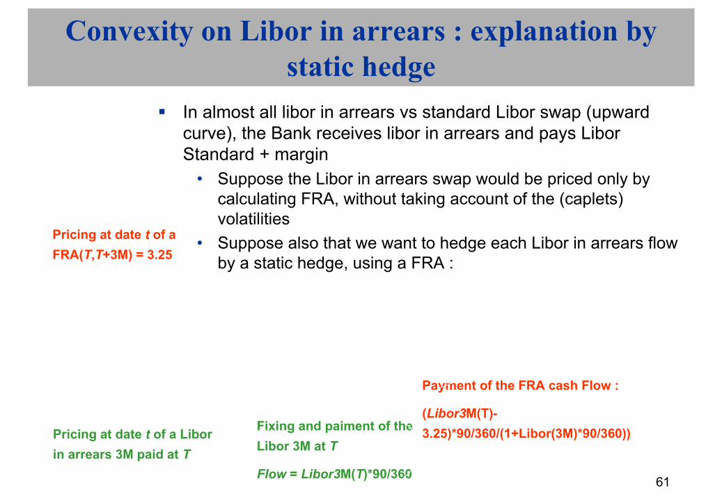
Convexity on Libor in arrears : explanation by static hedge
In almost all libor in arrears vs standard Libor swap (upwardcurve), the Bank receives libor in arrears and pays Libor Standard + margin
• Suppose the Libor in arrears swap would be priced only by calculating FRA, without taking account of the (caplets) volatilities
• Suppose also that we want to hedge each Libor in arrears flow by a static hedge, using a FRA :
Payment of the FRA cash Flow :
(Libor3M(T)-3.25)*90/360/(1+Libor(3M)*90/360))Pricing at date t of a Libor
in arrears 3M paid at T
t
Fixing and paiment of the Libor 3M at T
Flow = Libor3M(T)*90/360
T T+3M
Pricing at date t of a FRA(T,T+3M) = 3.25
62
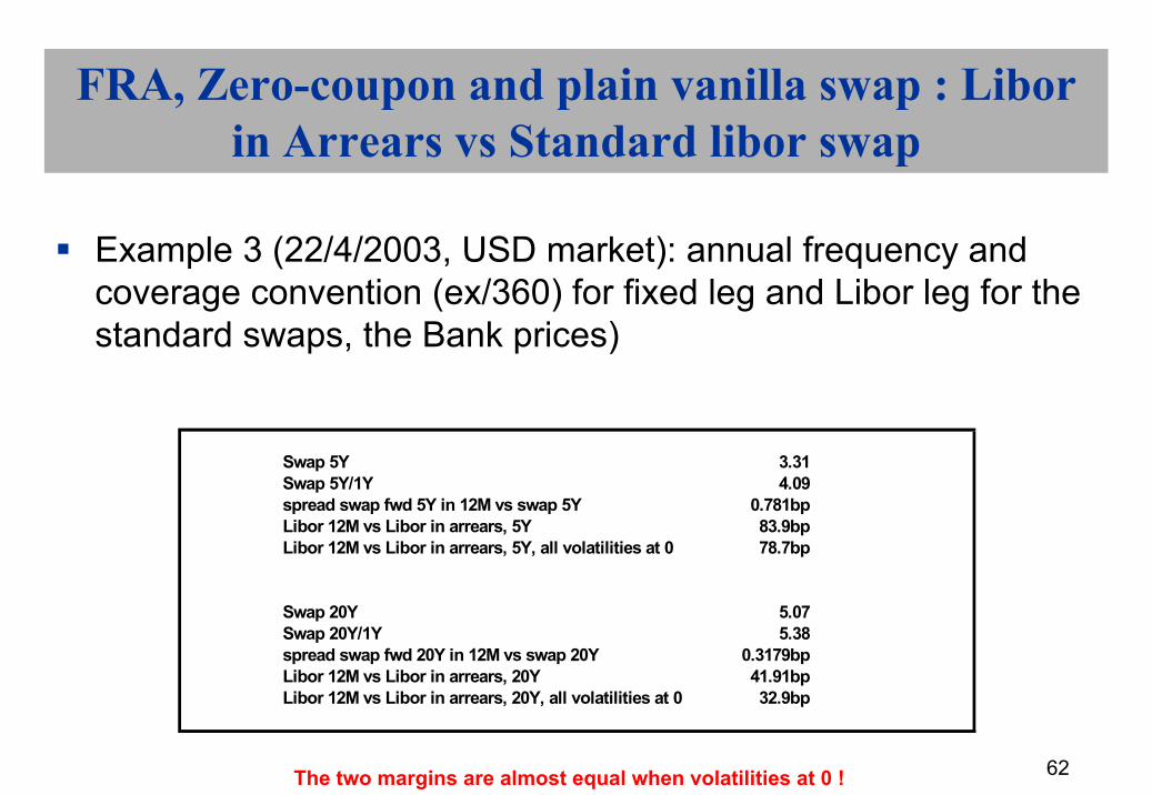
FRA, Zero-coupon and plain vanilla swap : Libor in Arrears vs Standard libor swap
Example 3 (22/4/2003, USD market): annual frequency and coverage convention (ex/360) for fixed leg and Libor leg for thestandard swaps, the Bank prices)
Swap 5Y 3.31Swap 5Y/1Y 4.09spread swap fwd 5Y in 12M vs swap 5Y 0.781bpLibor 12M vs Libor in arrears, 5Y 83.9bpLibor 12M vs Libor in arrears, 5Y, all volatilities at 0 78.7bp
Swap 20Y 5.07Swap 20Y/1Y 5.38spread swap fwd 20Y in 12M vs swap 20Y 0.3179bpLibor 12M vs Libor in arrears, 20Y 41.91bpLibor 12M vs Libor in arrears, 20Y, all volatilities at 0 32.9bp
The two margins are almost equal when volatilities at 0 !

63
Convexity on Libor in arrears : explanation by static hedge
Hedge ratio Libor in arrears/FRAObviously, the hedge ratio calculated at time t would be :
If we keep a constant hedge ratio, the Bank P&L at T will be :
( ) 0081251360902531 ./*. =+
( ) ( ) 008125.1
36090)M(31
3.25-)M(3360903.25-)M(3
36090
×
×+
×−×TLibor
TLiborTLibor

64
Convexity on Libor in arrears : explanation by static hedge
P&L of Bank, 3M in arrears with static hedge in FRA 3M
0
0.001
0.002
0.003
0.004
0.005
0.006
0.007
0.50% 1.50% 2.50% 3.50% 4.50% 5.50% 6.50%
Libor3M at the fixing
P&L
Ban
k, in
M E
UR

65
Convexity on Libor in arrears : explanation by static hedge
P&L of the Bank in function of Libor3M(T)As we see on the previous graph, of course at 0 if Libor3M(T)=3.25%, is positive whatever the value of Libor3M(T).It means that this time, the Bank is long the convexity, I.e or equivalently long of caplet volatilitiesThe higher the caplet vol, the higher the convexity adjustement

66
Convexity on Libor in arrears : explanation by static hedge
the Bank will have to sell options to pay the additional margin due to vol, and to dynamically manages this position. the Bank can also managing the position so as to be constantly delta-neutral and generate a positive P&L thanks to the convexity. In practice, of course, there is a global delta, gamma, vega…management of IR derivatives.
67
Convexity on CMS : explanation by static hedgeCMS pricing by replicationConvexity on Libor in arrears : explanation by static hedgeQuanto effect : correlation impact when rebalancing hedge
portfolio ; case study : Forward, Quanto swapOther convexity effect : future vs forward
68
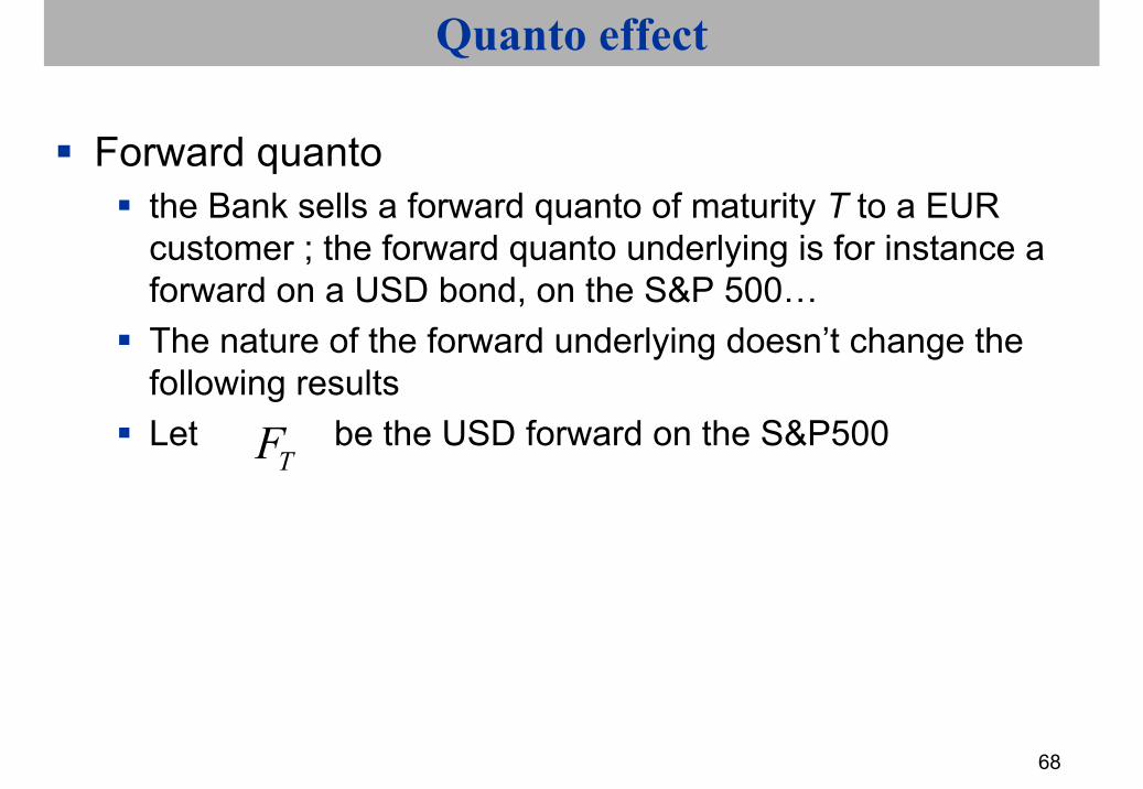
Quanto effect
Forward quantothe Bank sells a forward quanto of maturity T to a EUR customer ; the forward quanto underlying is for instance a forward on a USD bond, on the S&P 500…The nature of the forward underlying doesn’t change the following resultsLet be the USD forward on the S&P500
TF
69
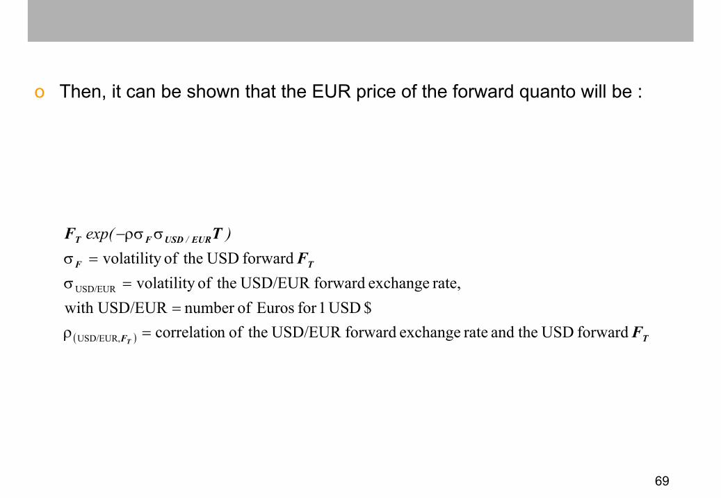
o Then, it can be shown that the EUR price of the forward quanto will be :
( ) TF
TF
EURUSDFT
F
FTF
T forward USD theand rate exchange forward USD/EUR theofn correlatio
$ USD1for Euros ofnumber URwith USD/E rate, exchange forward USD/EUR theof volatility
forward USD theof volatility
USD/EUR,
USD/EUR
=ρ=
=σ=σ
σρσ− )exp( /

70
Quanto effect
Important warning :The convention used for the FX exchange rate is not the market convention for quanto product with USD underlying and pay-off in EUR : the FX rate used is USD/EUR and not EUR/USD.For quanto product with underlying in EUR or USD and pay-off in Yen, the market convention and quanto convention are the same (EUR/YEN).

71
Quanto effect : an example
Numerical application : fwd 2A S&P 500 = 940, vol S&P = 23%, vol USD/EUR = 11%, correl (2A USD/EUR, 2A S&P500) = 0.6 fwd S&P 500 = 909.4
⇒
fwd quanto S&P 500 2A as a fucntion of correlation between fwd 2A USD/EUR and fwd 2A S&P 500
880
900
920
940
960
980
1000
-1 -0.8 -0.6 -0.4 -0.2 0 0.2 0.4 0.6 0.8 1
correlation
fwd
quan
to
fwd S&P 2A = 940

72
Quanto effect : interpretation
InterpretationSuppose first the correlation between forward USD/EUR and the forward S&P 500 is +1 :
Correlation = +1 means = that if the US $ falls, then the forward falls, if the US $ goes up then the forward goes up. Each time the S&P500 goes up by 1%, a EUR investor in the standard forward also makes a currency profit ($ goes up), each time the S&P500 goes down by 1%, the EUR investor makes a loss but the effect of the $ decline is then favorable. If the EUR investor buys a forward quanto, he doesn’t benefits from the correlation effect. Of course, P&L the Bank = -P&L client.
TF

73
Quanto effect : interpretation
Conclusion for a deal quanto such that currency of payment = EUR, currency underlying = USD
( )
( )
USD1per EUR ofnumber : USD/EUR
USDforward quanto forward0
USDforward quanto forward0
EUR/USD,
EUR/USD,
≤⇒≥
>⇒<
T
T
F
F
ρ
ρ
P&L EUR clientfwd standard fwd quanto
fwd S&P500 up 10%, $ fwd up 5% 10.50% 10%fwd S&P500 down-10%, $ fwd down -2.5% -9.75% -10%

74
Quanto : swap quanto
Swap Libor USD paid in EUR + margin vs Libor EUR
•Libor USD 6M vs EURIBOR 6M
•correl > 0 = if USD Libor falls, $ falls vs EUR
EUR annuel 30/360 USD Semi 30/360 correl -0.3 correl 0 correl 0.32y 2.3 1.495 76 78 80.255y 3.06 2.695 25.5 34 42.2510y 3.905 3.7575 -5.6 11 26.5
75
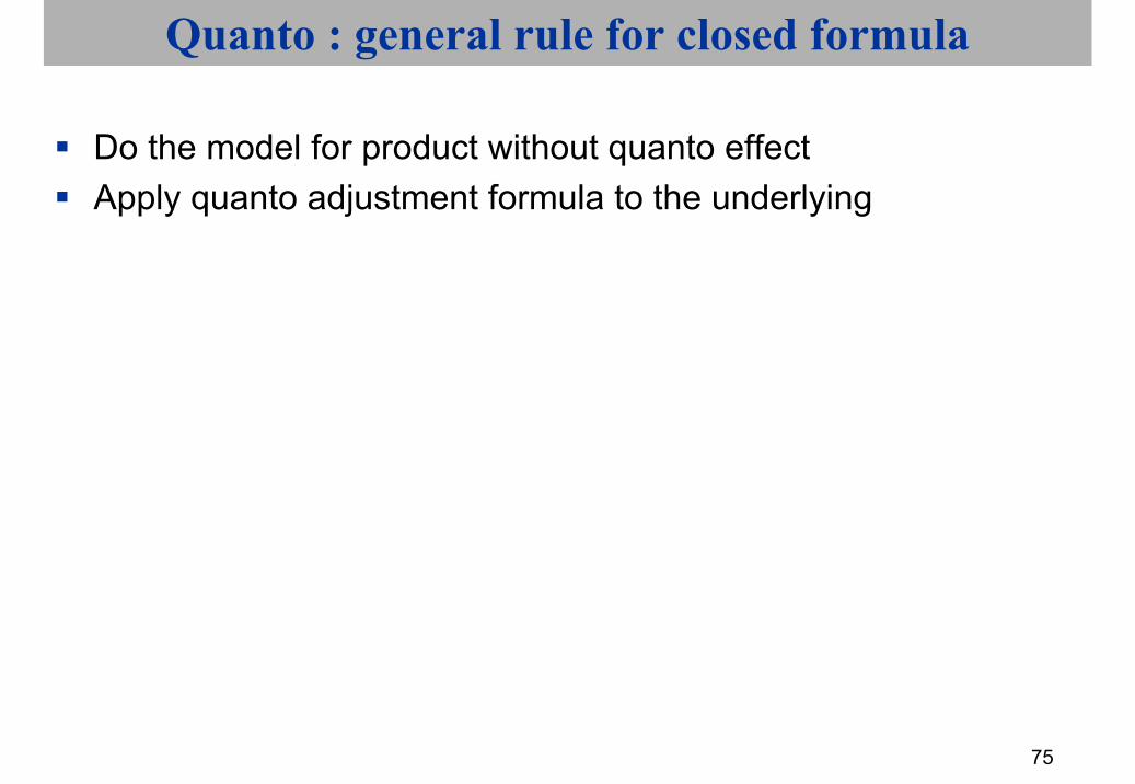
Quanto : general rule for closed formula
Do the model for product without quanto effectApply quanto adjustment formula to the underlying
76
Convexity on CMS : explanation by static hedgeCMS pricing by replicationConvexity on Libor in arrears : explanation by static hedgeQuanto effect : correlation impact when rebalancing hedge
portfolio ; case study : Forward, Quanto swapOther convexity effect : future vs forward

77
Other convexity effect : future vs forward
Reminder :Forward : contract of maturity T where the price you will buy underlying S at T is fixed at date 0.
Remark : some forward are with real physical delivery of underlying, other are forwards with cash-settlement
Future : contract of maturity T on underlying S whose price at T will be S(T) is fixed in continuous time with a call-margin system :
If price at t is F(t,T), price at t+dt is F(t,T+dt), the buyer receives F(t,T+dt)-F(t,T) at date t+dt and so on untill T.
78
Other convexity effect : future vs forward
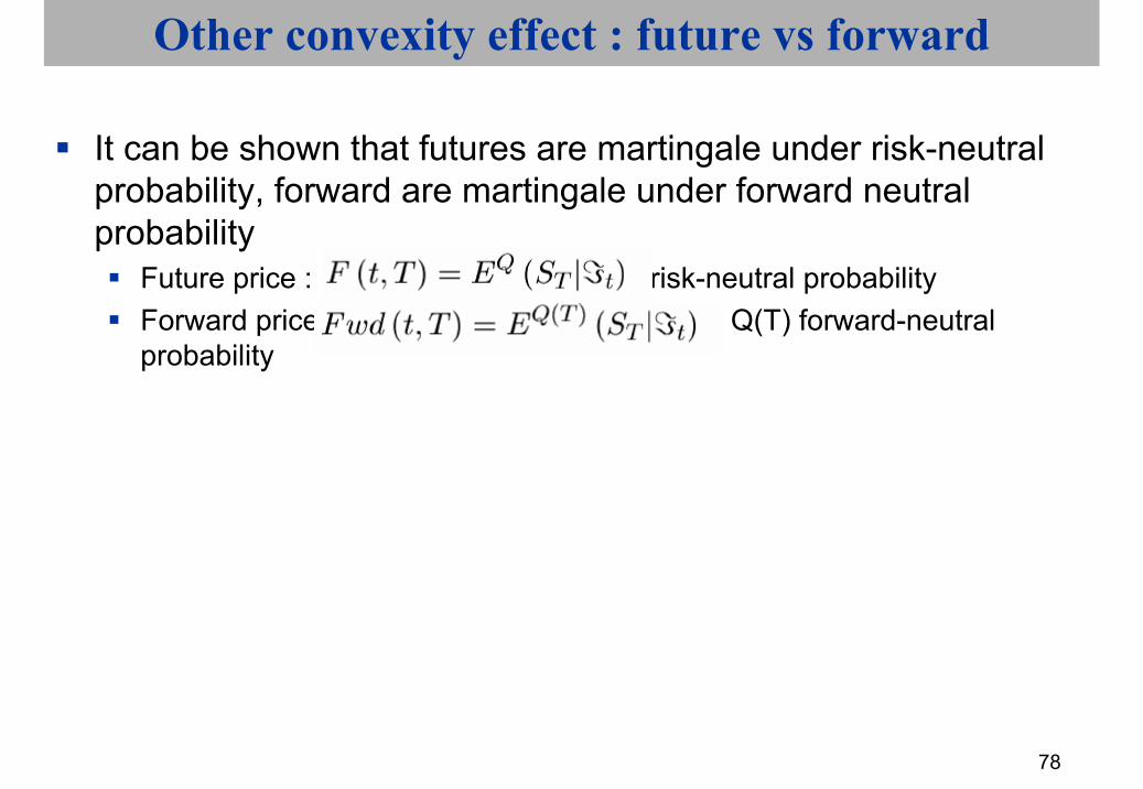
It can be shown that futures are martingale under risk-neutral probability, forward are martingale under forward neutral probability
Future price : , Q risk-neutral probabilityForward price : , Q(T) forward-neutral probability

79
Other convexity effect : future vs forward
Pricing :the forward price of assets needs no modelling, you just need :
Today underlying priceToday yield curveDividends for equities or coupon for bonds
Example : The forward price at t for date T of an asset S with no dividend and no coupon is (r continous zero-coupon rate) :
If there is a dividend yield a :

80
Other convexity effect : future vs forward
Future : if interest rates are assumed to be deterministic, future price = forward priceIt has been shown that :
If short rate and future processes are both gaussian, this formula is simpler ! :

81
Other convexity effect : future vs forward
In practice : F(t,T)-Fwd(t,T)=ρσ(r)σ(F)F(t,T)(T-t)ρ correlation between short rate and futureσ(r) standard deviation of the short rateσ(F) volatility of the futureAll these numbers are assumed constant

82
Other convexity effect : future vs forward
Hedge between futures and forwards :In order to hedge on forward of maturity T, sell
To get this formula no need complex maths, just need to know the difference between one dollar today and one dollar at T!

83
Other convexity effect : future vs forward
Future-Forward spread interpretation : What happens if correlation between short rate and future is -1 ?
Assume you buy one future, short rate is 4%Second day short rate is 4.5%, future is 99
Margin call -1 you must borrow at 4.5%Third day short rate at 4%, margin call at +1Fourth day short rate 3.5, margin call at +1…
When rates are low positive margin calls, when rate are high negative margin calls
84
Other convexity effect : future vs forward
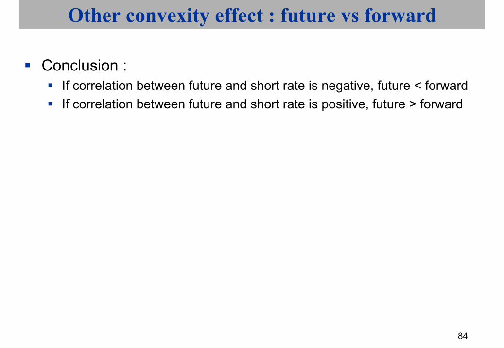
Conclusion : If correlation between future and short rate is negative, future < forwardIf correlation between future and short rate is positive, future > forward
85
Other convexity effect : future vs forward
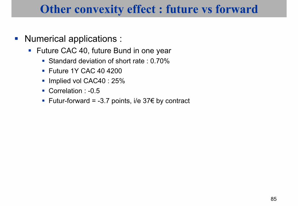
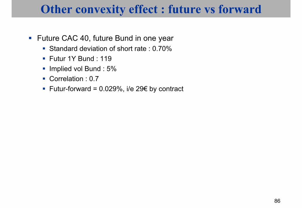
Numerical applications :Future CAC 40, future Bund in one year
Standard deviation of short rate : 0.70%Future 1Y CAC 40 4200Implied vol CAC40 : 25%Correlation : -0.5Futur-forward = -3.7 points, i/e 37€ by contract
86
Other convexity effect : future vs forward
Future CAC 40, future Bund in one yearStandard deviation of short rate : 0.70%Futur 1Y Bund : 119Implied vol Bund : 5%Correlation : 0.7Futur-forward = 0.029%, i/e 29€ by contract

87
Other convexity effect : future vs forward
Futures on equity index or bonds are not very liquid over 6 months and correlation are not easy to estimate
Is there any significant and real application of this formula in financial markets ?Yes : futures on 3M interest rates !

88
Other convexity effect : future vs forward
Futures eurodollars (or euribor, or Libor Yen, GBP..)Futures on (100-3M Libor $*100)We apply the previous formula, in the following HJMframework :
This is the simplest version of HJM ! (modern version of merton or vasicek model!)

89
Other convexity effect : future vs forward
It can be shown that spread between future and forward is then :
In addition the forward price is :
The forward price is slightly above the forward yield you can calculate using the yield curve!
90
Other convexity effect : future vs forward
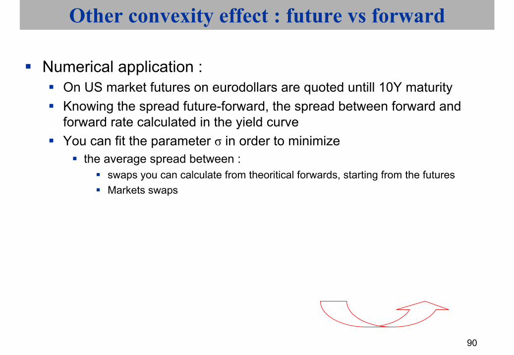
Numerical application : On US market futures on eurodollars are quoted untill 10Y maturityKnowing the spread future-forward, the spread between forward and forward rate calculated in the yield curveYou can fit the parameter σ in order to minimize
the average spread between :swaps you can calculate from theoritical forwards, starting from the futuresMarkets swaps
91
Other convexity effect : future vs forward
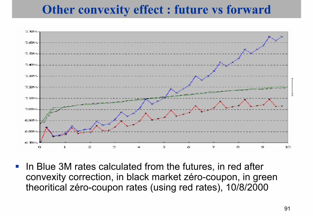
In Blue 3M rates calculated from the futures, in red after convexity correction, in black market zéro-coupon, in green theoritical zéro-coupon rates (using red rates), 10/8/2000

92
Other convexity effect : future vs forward
In blue theoritical swaps, in red market swaps, in black the spreads.

93
Other convexity effect : future vs forward
Historical value of implied σ : january 1994 to august 2000

94
Other convexity effect : future vs forward
So despite a very simple model (gaussian rates, constant standard deviation, one factor), you fit very well the markets !In real markets, the FRA (forward rate agreement) on deposits rates contracts are cash-settled with the following pay-off at T:
95
Other convexity effect : future vs forward
Where FRA is the initial price of the forward, V(T) the final value of the deposit rate between T and T* at T.
It can be shown easily that the theoritical price of the forward is the theforward rate you can calculate using the yield curveFortunately, this is the market practice !
In conclusion, the spread between future-forward on eurodollars contracts is essentially :
Future –forward effectResidual convexity effect (convexity relation between 3M rates and 3M zéro-coupon bond).

96
Annex 1 : Convex one variable functions
Graphic definitionA function is convex if the surface above its graph is convex, i.e if wetake two points in this surface, each point of the segment defined by thistwo points belongs to the surface.
-1
-0.5
0
0.5
1
1.5
2
2.5
3
3.5
4
4.5
5
5.5
6
6.5
7
7.5
8
8.5
-13 -8 -3 2 7 12
A
B
97
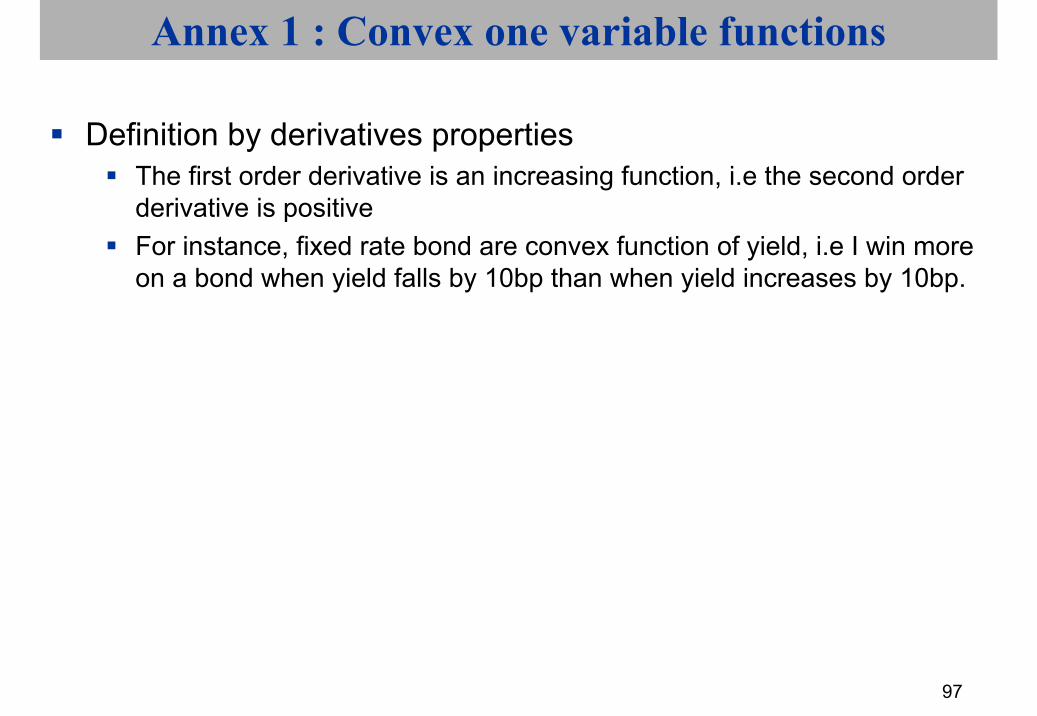
Annex 1 : Convex one variable functions
Definition by derivatives propertiesThe first order derivative is an increasing function, i.e the second order derivative is positiveFor instance, fixed rate bond are convex function of yield, i.e I win more on a bond when yield falls by 10bp than when yield increases by 10bp.
98
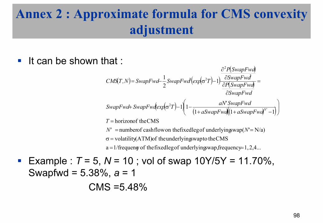
Annex 2 : Approximate formula for CMS convexityadjustment
It can be shown that :
Example : T = 5, N = 10 ; vol of swap 10Y/5Y = 11.70%, Swapfwd = 5.38%, a = 1
CMS =5.48%
( ) ( )( )( )
( )
( )( )( ) ( )( )
2,4... 1, frequencyswap, underlying of leg fixed theofy 1/frequenc aCMS the toswap underlying theof (ATM) volatility
N/a)'( swap underlying of leg fixed on the flowcash ofnumber CMS theofhorizon
11111
121
2
2
2
22
===σ
===
−++−−σ+
=
∂∂∂
∂
−σ−=
N 'NT
aSwapFwdaSwapFwdSwapFwd'aNTexpSwapFwdSwapFwd
SwapFwdSwapFwdP
SwapFwdSwapFwdP
TexpSwapFwdSwapFwdN,TCMS
'N