Convergence Prospects for CEE Countries M. Sc. Dissertation Paper ACADEMY OF ECONMIC STUDIES...
34
Convergence Prospects for CEE Countries M. Sc. Dissertation Paper ACADEMY OF ECONMIC STUDIES DOCTORAL SCHOOL OF FINANCE AND BANKING Mihaescu Flaviu Coordinator: Professor Moisa Altar
-
Upload
thomasine-nichols -
Category
Documents
-
view
216 -
download
1
Transcript of Convergence Prospects for CEE Countries M. Sc. Dissertation Paper ACADEMY OF ECONMIC STUDIES...

Convergence Prospects for CEE Countries
M. Sc. Dissertation Paper
ACADEMY OF ECONMIC STUDIES
DOCTORAL SCHOOL OF FINANCE AND BANKING
Mihaescu Flaviu
Coordinator: Professor Moisa Altar

Convergence:Hypotheses
•Poor countries catch-up with the rich ones.
•The farther the initial level of (per capita) output from the steady state, the faster the growth.
0,0,, )1
()ln(ln1
i
T
iTi YT
eaYY
T
•Equation:

Convergence:Major drawbacks
•“Steady states”: different countries have different steady states
•Unconditioned convergence holds only for some countries / regions
•E.g.: U.S. states, Japanese prefectures and OECD regions
•They have the same steady states

Conditional Convergence
•Conditional convergence accounts for different steady states
•Conditioning variables may be:
•Government consumption
•Domestic savings
•Domestic investments

Conditional Convergence
•Equation:
0,0,0,, )1
()ln(ln1
ii
T
iTi XYT
eaYY
T
•Empirical evidence:
•Barro and Sala-i-Martin (1991),
•Mankiw, Romer and Weil (1990),
•Sachs and Warner (1995)

Unconditional Convergence: CEEC11
Premises for convergence:
•the same pattern of output growth
•EU accession candidates and proximity
•converging structure of the economies
•legislative and institutional approximation
•openness of trade
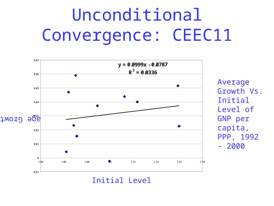
Unconditional Convergence: CEEC11
Average Growth
Initial Level
y = 0.0999x - 0.0787
R2 = 0.0336
-0.01
0
0.01
0.02
0.03
0.04
0.05
0.06
0.07
1.04 1.06 1.08 1.1 1.12 1.14 1.16 1.18
Average Growth Vs. Initial Level of GNP per capita, PPP, 1992 - 2000

Conditional Convergence:Accounting for Different Steady-States
•Split the 11 countries group by EU - Accession criteria:
1998 Group:
Poland, Czech Republic, Estonia, Hungary and Slovenia
2000 Group:
Bulgaria, Lithuania, Latvia, Romania, Slovak Republic
plus Croatia

Conditional Convergence:Accounting for Different Steady-States
•The 1998 Group1998 Group will have the per capita income level of SpainSpain as steady state (about 80% of EU level)
•The 2000 Group2000 Group will have the per capita income level of GreeceGreece as steady state (about 60% of EU level)

Conditional Convergence:Accounting for Different Steady-States
The highlighted countries are those from the 1998 group and their per-capita GNP was divided by Spain’s. The rest – not highlighted – are the 2000 group countries plus Croatia and they have Greece as steady state.
Relative Per CapitaIncome Level as a %
of Steady State
Relative Per CapitaIncome Level as a% of EU Average
1992 2000 2000Bulgaria 39.87 42.40 25.1Croatia 40.56 53.71 31.8Czech Republic 79.17 80.38 63.1Estonia 44.95 66.72 39.5Hungary 59.25 69.94 54.9Latvia 42.01 49.66 29.4Lithuania 53.86 50.66 30.0Poland 38.68 51.97 40.8Romania 42.91 46.62 27.6Slovak Republic 59.76 61.91 48.6Slovenia 78.57 97.32 76.4
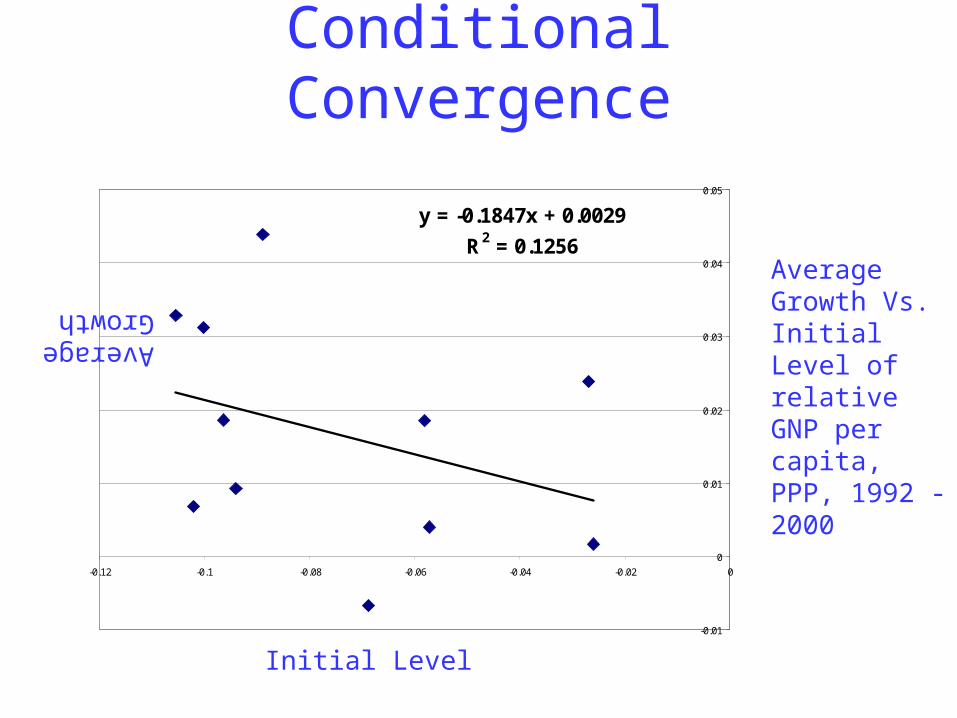
Conditional Convergence
y = -0.1847x + 0.0029
R2 = 0.1256
-0.01
0
0.01
0.02
0.03
0.04
0.05
-0.12 -0.1 -0.08 -0.06 -0.04 -0.02 0
Average Growth
Initial Level
Average Growth Vs. Initial Level of relative GNP per capita, PPP, 1992 - 2000
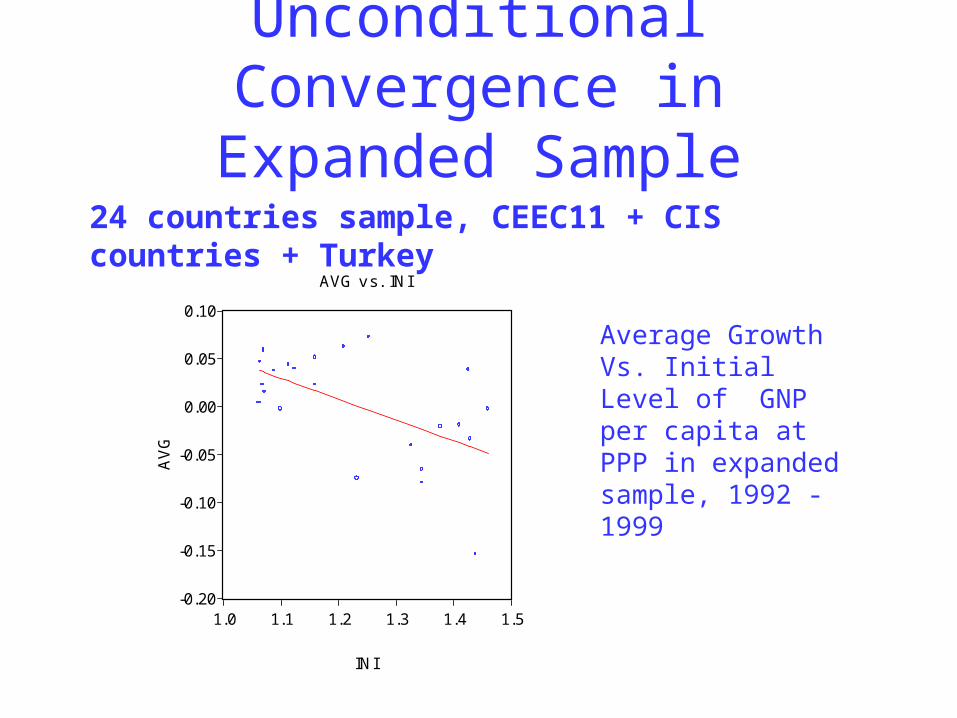
Unconditional Convergence in Expanded Sample
24 countries sample, CEEC11 + CIS countries + Turkey
-0.20
-0.15
-0.10
-0.05
0.00
0.05
0.10
1.0 1.1 1.2 1.3 1.4 1.5
INI
AV
G
AVG v s. INI
Average Growth Vs. Initial Level of GNP per capita at PPP in expanded sample, 1992 - 1999

Unconditional Convergence in Expanded Sample
CISInieaAvg T )1(
Regression output
(CIS is a dummy variable for CIS countries):
with 2153.0a 0239.0 and 0463.0 Adj. R-sqr = 0.4225
(0.0139) (0.0478) (0.0259) Prob. (F-Stat.) = 0.0016
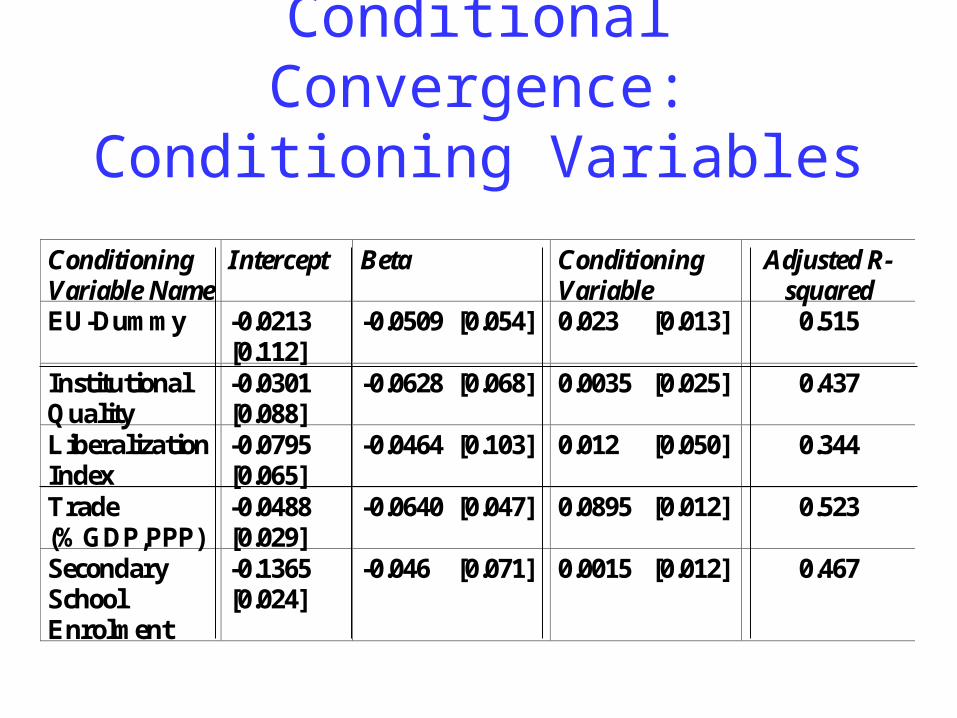
Conditional Convergence:Conditioning Variables
ConditioningVariable Name
Intercept Beta ConditioningVariable
Adjusted R-squared
EU-Dummy -0.0213[0.112]
-0.0509 [0.054] 0.023 [0.013] 0.515
InstitutionalQuality
-0.0301[0.088]
-0.0628 [0.068] 0.0035 [0.025] 0.437
LiberalizationIndex
-0.0795[0.065]
-0.0464 [0.103] 0.012 [0.050] 0.344
Trade(%GDP,PPP)
-0.0488[0.029]
-0.0640 [0.047] 0.0895 [0.012] 0.523
SecondarySchoolEnrolment
-0.1365[0.024]
-0.046 [0.071] 0.0015 [0.012] 0.467

Conditional Convergence:Conditioning Variables
InstQTradeInieaAvg T 21)1(
With a = -0.06 β = -0.089 γ1 = 0.068 γ2 = 0.0025
[0.005] [0.017] [0.019] [0.037]
R - sqr. = 0.803 F-stat. = 9.539 [0.007]
Adj. R - sqr. = 0.719

Conditional Convergence:Conditioning Variables
•“Institutional QualityInstitutional Quality” comprises voice and accountability, politically instability and violence, government effectiveness, regulatory burden, rule of law and graft.
•“TradeTrade” is the sum of imports and exports divided by GDP, all at PPP, and it is often taken as a measure of openness.

Timing Convergence
•The 1998 group (Czech Republic, Estonia, Hungary, Poland and Slovenia) will reach Spain or approximately 80 percent of EU average per capita income in 16 – 18 years
•The 2000 group (Bulgaria, Latvia, Lithuania, Slovak Republic, Romania plus Croatia) will reach Greece or approximately 60 percent of EU average income also in 16 – 18 years.

Scenario Analysis
Assumptions:
•“Trade” will increase with one Standard Deviation
•“Institutional Quality”: the 1998 Group will improve their institutional quality with 2 points, while the 2000 Group will improve with 4 points.
•“Optimistic” scenario assumes a 9% speed of convergence, the “pessimistic” one a 2.4%, while the “intermediate” one assumes 6%.

Scenario Analysis
Country Trade St. Dev. Trade +1 St. Dev.
Institutional Quality
Increase New Inst.Q. Level
BLG 0.2329 0.0243 0.2572 0.1 4 4.1
HRV 0.4087 0.0357 0.4444 0.3 4 4.3
CZ 0.3852 0.0658 0.4511 6.8 2 8.8
EST 0.5720 0.1407 0.7127 6.1 2 8.1
HUN 0.3850 0.0887 0.4738 8.7 2 10.7
LAT 0.2971 0.0742 0.3713 2.6 4 6.6
LIT 0.349 0.090 0.4392 2.6 4 6.6
POL 0.2232 0.0513 0.2745 7.0 2 9
ROM 0.1336 0.0237 0.1574 -0.8 4 3.2
SVK 0.3982 0.0572 0.4553 2.8 4 6.8
SVN 0.6336 0.0533 0.6869 8.5 2 10.5
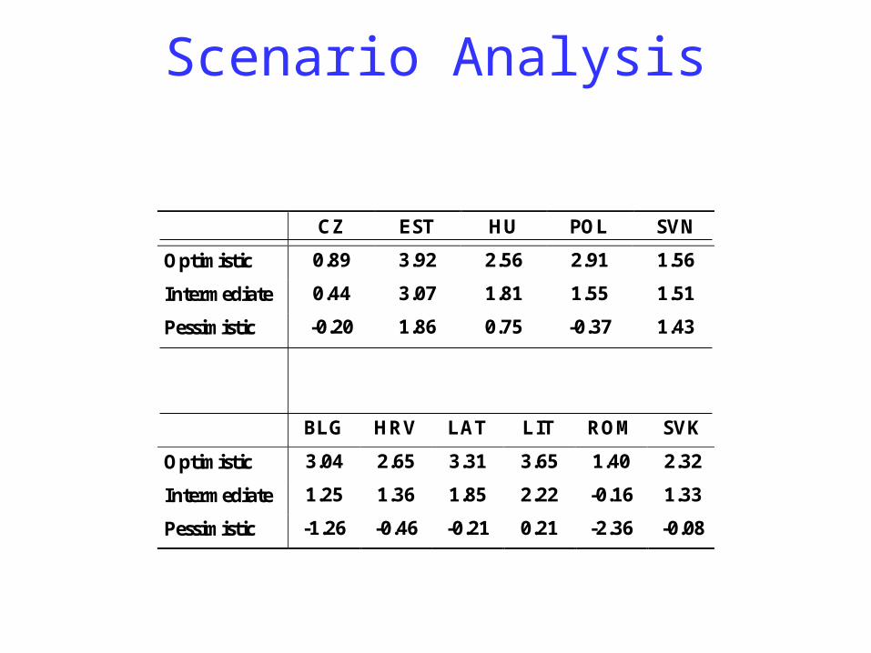
Scenario Analysis
CZ EST HU POL SVN
Optimistic 0.89 3.92 2.56 2.91 1.56
Intermediate 0.44 3.07 1.81 1.55 1.51
Pessimistic -0.20 1.86 0.75 -0.37 1.43
BLG HRV LAT LIT ROM SVK
Optimistic 3.04 2.65 3.31 3.65 1.40 2.32
Intermediate 1.25 1.36 1.85 2.22 -0.16 1.33
Pessimistic -1.26 -0.46 -0.21 0.21 -2.36 -0.08
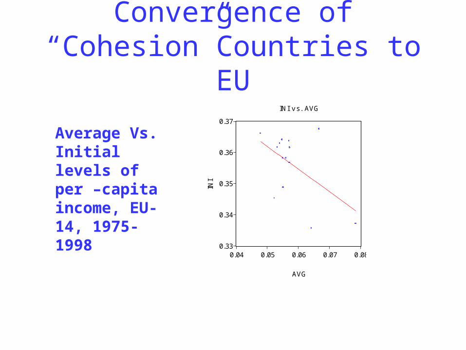
Convergence of “Cohesion”Countries to EU
0.33
0.34
0.35
0.36
0.37
0.04 0.05 0.06 0.07 0.08
AVG
INI
INI v s. AVG
Average Vs. Initial levels of per –capita income, EU-14, 1975-1998

Convergence of “Cohesion”Countries to EU
DUMDIGCIniaAvg 321
Conditioning variables:
a = -0.37 β = -0.281 γ1 = 0.051 γ2 = 0.082 γ3 = -0.021
[0.006] [0.077] [0.013] [0.003]
R - sqr. = 0.809 Adj. R - sqr. = 0.777
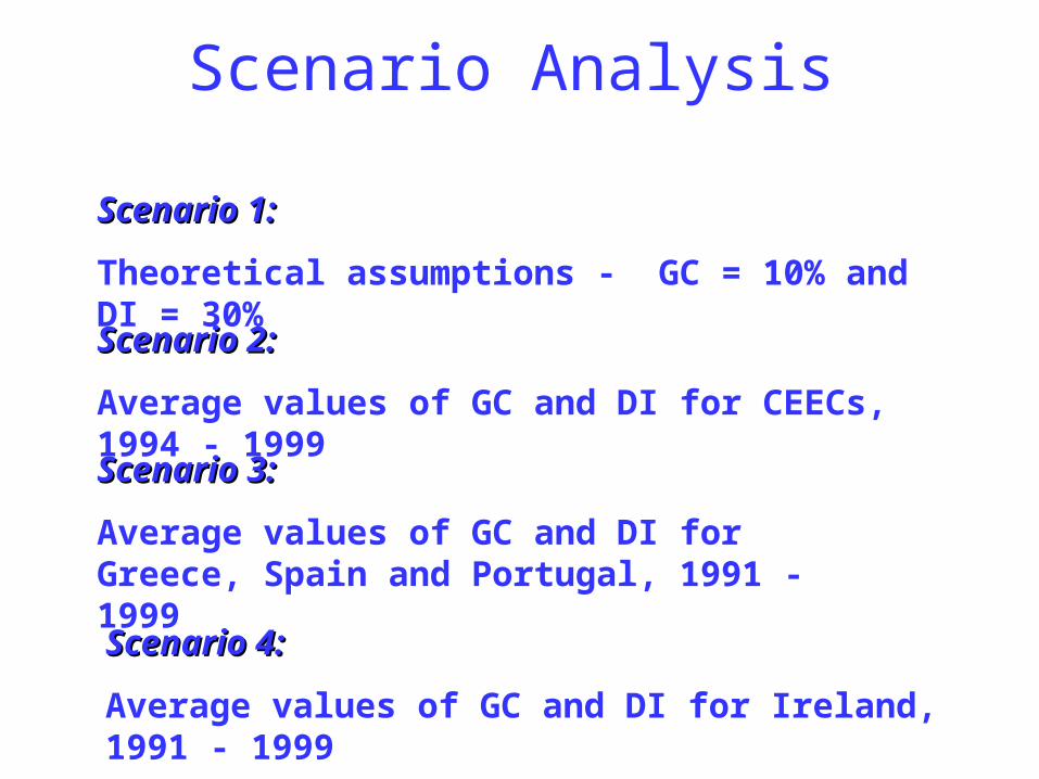
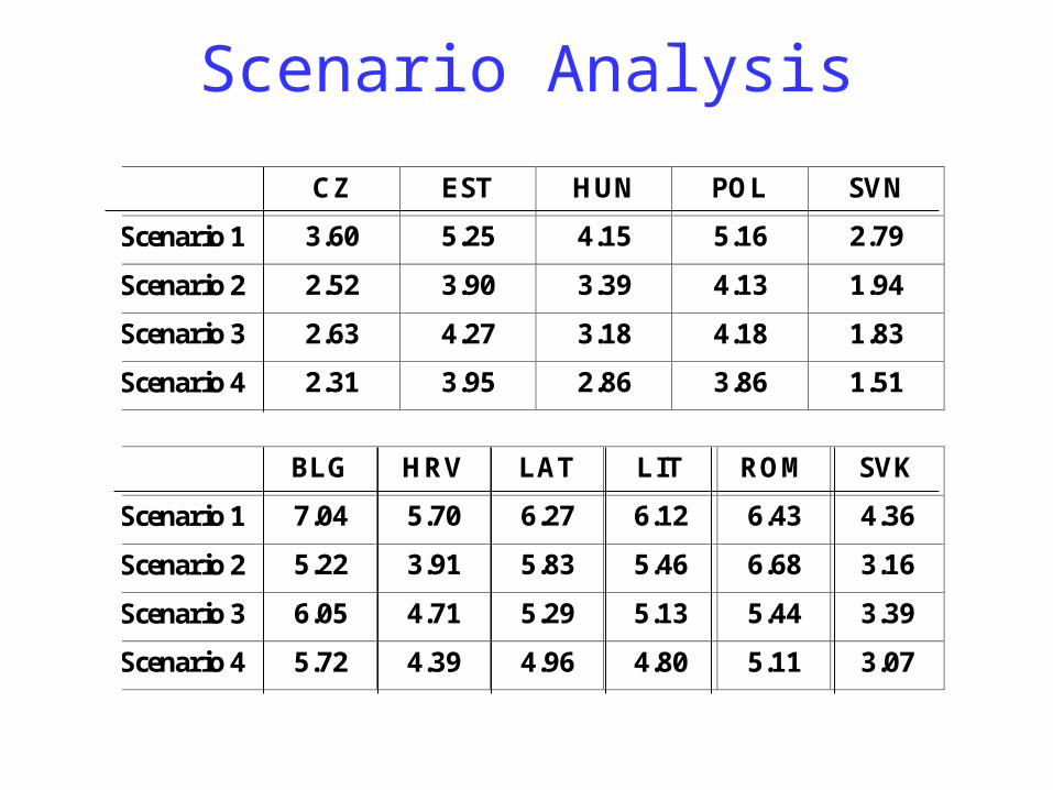
Scenario Analysis
Scenario 1:Scenario 1:
Theoretical assumptions - GC = 10% and DI = 30%
Scenario 2:Scenario 2:
Average values of GC and DI for CEECs, 1994 - 1999
Scenario 3:Scenario 3:
Average values of GC and DI for Greece, Spain and Portugal, 1991 - 1999
Scenario 4:Scenario 4:
Average values of GC and DI for Ireland, 1991 - 1999
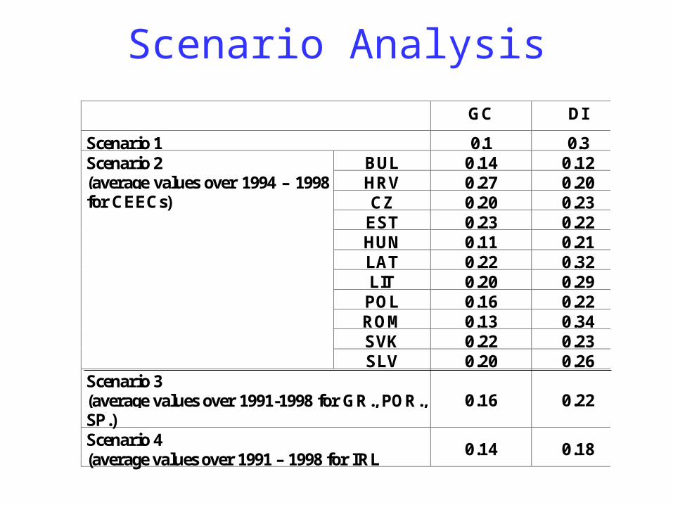
Scenario Analysis
GC DI
Scenario 1 0.1 0.3BUL 0.14 0.12HRV 0.27 0.20CZ 0.20 0.23
EST 0.23 0.22HUN 0.11 0.21LAT 0.22 0.32LIT 0.20 0.29
POL 0.16 0.22ROM 0.13 0.34SVK 0.22 0.23
Scenario 2(average values over 1994 – 1998for CEECs)
SLV 0.20 0.26Scenario 3(average values over 1991-1998 for GR., POR.,SP.)
0.16 0.22
Scenario 4(average values over 1991 – 1998 for IRL
0.14 0.18
Scenario Analysis
CZ EST HUN POL SVN
Scenario 1 3.60 5.25 4.15 5.16 2.79
Scenario 2 2.52 3.90 3.39 4.13 1.94
Scenario 3 2.63 4.27 3.18 4.18 1.83
Scenario 4 2.31 3.95 2.86 3.86 1.51
BLG HRV LAT LIT ROM SVK
Scenario 1 7.04 5.70 6.27 6.12 6.43 4.36
Scenario 2 5.22 3.91 5.83 5.46 6.68 3.16
Scenario 3 6.05 4.71 5.29 5.13 5.44 3.39
Scenario 4 5.72 4.39 4.96 4.80 5.11 3.07

σ - Convergence
•Output gap between the group members decline over time
•σ - convergence does dot imply β - convergence, nor conversely
•“catch-up at the top and downward convergence at the bottom” (Ben- David, 1997)
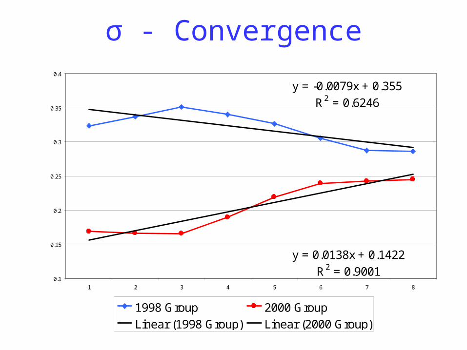
σ - Convergence
y = -0.0079x + 0.355
R2 = 0.6246
y = 0.0138x + 0.1422
R2 = 0.90010.1
0.15
0.2
0.25
0.3
0.35
0.4
1 2 3 4 5 6 7 8
1998 Group 2000 Group
Linear (1998 Group) Linear (2000 Group)

σ - Convergence
Var(Group1998) = 0.347 - 0.0078 * trend [0.00] [0.02]
R – sqr = 0.56
Var(Group 2000) = 0.156 + 0.0138 * trend [0.00] [0.00]
R – sqr = 0.88
Variance trend for restricted sample, 1992 - 1999

Ergodic Distribution
•Considers the entire income distribution
•Follows Quah (1997)
• Transition probabilities matrix of moving from one income group to another. The diagonal probabilities show the probability of staying in the same income group, while the off-diagonal probabilities are the probabilities of moving from one income group to the subsequent one (up or down).

Ergodic Distribution
•The ergodic distribution is:
1lim
m
mP
Where P is the transition probabilities matrix.
•The ergodic distribution can be obtained as the left eigenvector corresponding to the unit eigenvalue. (Because each row of the matrix sums to one)
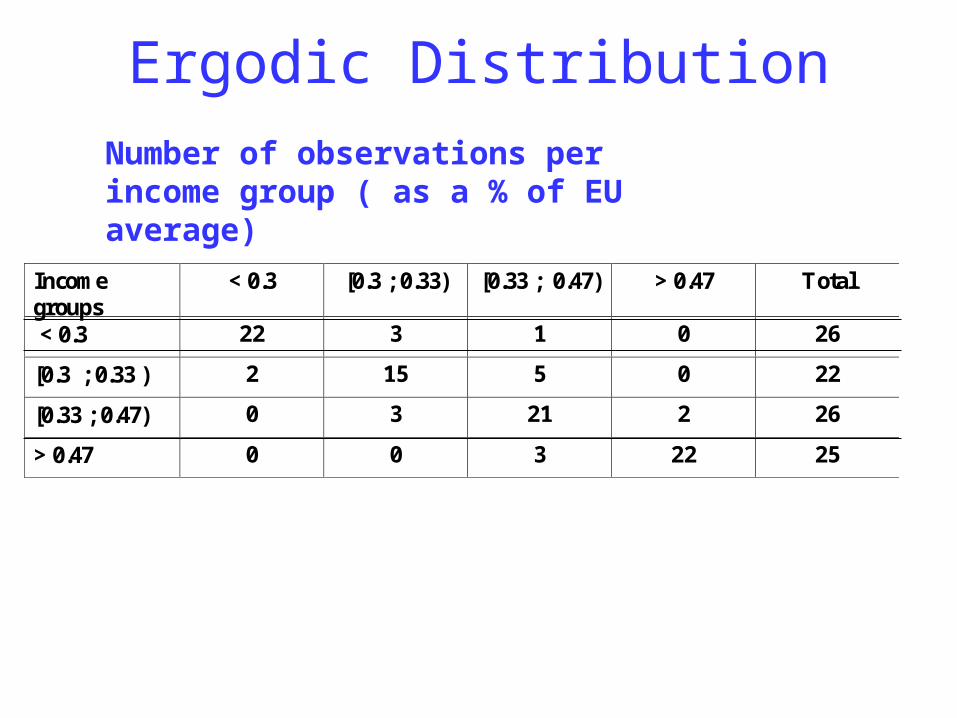
Ergodic Distribution
Incomegroups
< 0.3 [0.3 ; 0.33) [0.33 ; 0.47) > 0.47 Total
< 0.3 22 3 1 0 26
[0.3 ; 0.33 ) 2 15 5 0 22
[0.33 ; 0.47) 0 3 21 2 26
> 0.47 0 0 3 22 25
Number of observations per income group ( as a % of EU average)
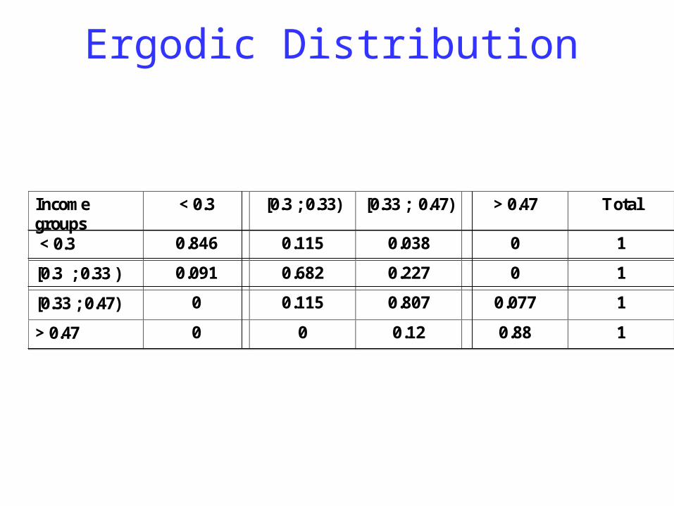
Incomegroups
< 0.3 [0.3 ; 0.33) [0.33 ; 0.47) > 0.47 Total
< 0.3 0.846 0.115 0.038 0 1
[0.3 ; 0.33 ) 0.091 0.682 0.227 0 1
[0.33 ; 0.47) 0 0.115 0.807 0.077 1
> 0.47 0 0 0.12 0.88 1
Ergodic Distribution
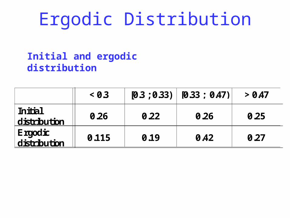
Ergodic Distribution
< 0.3 [0.3 ; 0.33) [0.33 ; 0.47) > 0.47
Initialdistribution
0.26 0.22 0.26 0.25
Ergodicdistribution
0.115 0.19 0.42 0.27
Initial and ergodic distribution
Conclusions
•β - convergence is achieved after controlling for different β - convergence is achieved after controlling for different steady statessteady states
• σ - convergence shows that there is rather divergence σ - convergence shows that there is rather divergence among 2000 Group countries, while 1998 Group among 2000 Group countries, while 1998 Group countries do also exhibit σ - convergence countries do also exhibit σ - convergence
•The ergodic distribution shows that there is convergence The ergodic distribution shows that there is convergence among CEEC 11 countries, namely the 2000 Group will among CEEC 11 countries, namely the 2000 Group will converge in per capita income to the 1998 Group.converge in per capita income to the 1998 Group.