Controllability and motion algorithms for underactuated ...andrew/papers/pdf/1997b.pdf ·...

IEEE Transactions on Automatic Control45(8), 1437–1454, 2000doi: 10.1109/9.8717532000 IEEE. Personal use of this material is permitted. However, permission to reprint/republish this material for advertising orpromotional purposes or for creating new collective works for resale or redistribution to servers or lists, or to reuse any copyrightedcomponent of this work in other works must be obtained from the IEEE

Controllability and motion algorithms for underactuatedLagrangian systems on Lie groups

Francesco Bullo∗ Naomi E. Leonard† Andrew D. Lewis‡

1997/11/29

Last updated: 1998/04/10

Abstract

In this paper, we provide controllability tests and motion control algorithms forunderactuated mechanical control systems on Lie groups with Lagrangian equal tokinetic energy. Examples include satellite and underwater vehicle control systems withthe number of control inputs less than the dimension of the configuration space. Localcontrollability properties of these systems are characterised, and two algebraic testsare derived in terms of the symmetric product and the Lie bracket of the input vectorfields. Perturbation theory is applied to compute approximate solutions for the systemunder small-amplitude forcing; in-phase signals play a crucial role in achieving motionalong symmetric product directions. Motion control algorithms are then designed tosolve problems of point-to-point reconfiguration, static interpolation and exponentialstabilisation. We illustrate the theoretical results and the algorithms with applicationsto models of planar rigid bodies, satellites and underwater vehicles.

Keywords. nonlinear control, mechanical systems, nonlinear controllability, underac-tuated systems.

AMS Subject Classifications (2010). 70E15, 70Q05, 93B05, 93B27.

1. Introduction

Underactuated mechanical control systems provide a challenging research area of in-creasing interest in both application and theory. In this paper, we examine an importantclass of underactuated mechanical control systems and address problems in both nonlinearcontrollability and nonlinear control design. It is precisely because we specialise to a richclass of mechanical systems that we can solve relevant controllability and control design

∗Associate Professor, Mechanical Engineering, University of California at Santa Barbara, En-gineering II Bldg., Santa Barbara, CA 93106-5070, U.S.A.Email: [email protected], URL: http://motion.mee.ucsb.edu/Work performed while a graduate student at the California Institute of Technology†Professor, Department of Mechanical and Aerospace Engineering, Princeton University,Princeton, NJ 08544, U.S.A.Email: [email protected], URL: http://www.princeton.edu/~naomi/‡Professor, Department of Mathematics and Statistics, Queen’s University, Kingston, ON K7L3N6, CanadaEmail: [email protected], URL: http://www.mast.queensu.ca/~andrew/Research performed while Research Fellow at the California Institute of Technology.Research in part supported by a grant from the Powell Foundation and by NSF Grant CMS–9502224.

1

http://dx.doi.org/10.1109/9.871753

2 F. Bullo, N. E. Leonard, and A. D. Lewis

problems; we derive controllability tests and motion control algorithms by making use ofthe mechanical system structure.

Underwater vehicles, satellites, surface vessels, airships and hovercraft are all examplesof simple mechanical control systems on Lie groups. For these systems, relevant Lagrangianmodels are available and lift/drag type effects are sometimes negligible. Key features are thefollowing: (1) the configuration space is a Lie group, as, for example, the group of rotationsSO(3) in the case of a satellite, (2) the Lagrangian is equal to the kinetic energy, and (3)external forces are fixed with respect to the body. From a theoretical perspective, thesesystems when underactuated offer a control challenge as they have non-zero drift (e.g., theirdynamics include Coriolis effects), their linearisation at zero velocity is not controllable, theyare not stabilisable by continuous state feedback and exponential stabilisation cannot beachieved by smooth time-varying feedback [M’Closkey and Murray 1997]. Further, theyare generically not nilpotent, not feedback linearisable, not “configuration flat,” as definedby Rathinam and Murray [1998], and no test is available to establish whether they aredifferentially flat. In other words, the motion planning and the stabilisation problem forthis class of systems cannot be solved with any established method.

We focus on this class of systems with fewer actuators than degrees of freedom, and westudy several motion control problems in the small-velocity range. From a practical pointof view, we are motivated by vehicles that are underactuated either because of an actuatorfailure or because of a design choice. In the former case, our results will improve robustnessto actuator failure and thus will provide autonomous vehicles with greater reliability. Inthe latter case, our results may allow for vehicle designs that include fewer actuators thantypical leading to lighter, less costly designs. Provided that certain controllability conditionsare satisfied, we show how underactuated vehicles can still perform important tasks suchas stabilisation (station keeping) and short range reconfigurations (parking, tracking).

Relevant past contributions include work on both the nonlinear controllability problemand the constructive controllability problem (including both motion planning and stabil-isation). For our work, the most important references for controllability are the worksof Sussmann [1987] on small-time local controllability and of Lewis and Murray [1997a](see also [Lewis and Murray 1997b]) on configuration controllability for simple mechanicalsystems. Other contributions include local controllability results for other classes of me-chanical systems, see [Kelly and Murray 1994] and [Ostrowski and Burdick 1997], and workon global controllability issues, see [Bonnard 1984], [Crouch 1984] and [Manikonda andKrishnaprasad 1997]. Regarding the constructive controllability problem, we employ thesame approach as Leonard and Krishnaprasad [1995] and Leonard [1995], where motion al-gorithms for a class of kinematic systems on Lie groups were designed with small-amplitudeperiodic inputs. In later work [Rui, Kolmanovsky, McNally, and McClamroch 1996] similartechniques were applied to a different class of mechanical system. Other contributions onoscillatory controls and Lagrangian systems include [Baillieul 1993, Gurvits 1992, Sussmannand Liu 1991]. A somewhat different approach, based on homogeneous time-varying strate-gies, was employed by Morin and Samson [1997] and Pettersen and Egeland [1997] to designexponentially stabilising control laws for underactuated satellites and surface vessels.

To derive controllability tests for our class of systems, we apply the controllability anal-ysis described by Sussmann [1987] and Lewis and Murray [1997a] to simple mechanicalcontrol systems on Lie groups (see also [Bullo and Lewis 1996]). Key features of the anal-ysis are a focus on the evolution of the system’s configuration when the initial velocity is

Underactuated Lagrangian systems on Lie groups 3

zero and the result that computations are performed on the Lie algebra of the Lie group.The local controllability properties are characterised by the algebraic operations of sym-metric product and Lie bracket. The symmetric product, which is defined more formallyin Section 2, depends upon the metric that defines the kinetic energy and, as we shall see,explicitly describes motions that involve both input vector fields and the drift dynamics.Our tests describe which velocities and configurations are reachable, independent of theinitial configuration. The notions of good and bad symmetric products play a central role.

Guided by our interpretation of the controllability tests, we apply perturbation theoryto investigate the response of the mechanical system to small-amplitude forcing. The initialvelocity is also assumed to have small amplitude. The approximations we obtain give furtherinsight into the controllability tests and are instrumental in the subsequent control design.Numerous examples illustrate the meaning of good and bad symmetric products and theeffects of in-phase and out-of-phase sinusoidal inputs.

On the basis of a controllability assumption, we design two motion primitives that per-form the basic tasks of changing and maintaining velocity. These motion primitives usein-phase inputs and compensate for contributions along bad symmetric product directions(see also [Bullo and Leonard 1997]). The two motion primitives synthesise the controllabil-ity analysis and are the building blocks for designing high-level motion procedures. Usingdiscrete-time feedback and multiple calls to the motion primitives, we design motion algo-rithms to solve the point-to-point reconfiguration problem (i.e., how to steer the system toa desired configuration) and the static interpolation problem (i.e., how to steer the systemthrough a set of desired configurations). We solve point-to-point reconfiguration using aconstant velocity algorithm. A second approach to point-to-point reconfiguration consists ofinterpolating a sequence of segments connecting initial to final configuration. We show theadvantage of the latter solution in the case the segments are steady motions of the unforcedmechanical system. Next, iterating an approximate stabilisation step we design an algo-rithm that locally exponentially stabilises the system to a desired configuration. Recall thatexponential stabilisation cannot be achieved by smooth time-varying feedback, and indeedour motion primitives are continuous, but not smooth, functions of the state. Accordingly,our approach relies on discrete-time continuous feedback, see [Sørdalen and Egeland 1995],and on the iteration of a motion planning step, see [Lafferriere and Sussmann 1991]. Fi-nally, the three algorithms are implemented numerically to verify the approximations andillustrate the control design.

The paper is organised as follows. In Section 2 we present some mathematical prelim-inaries and provide many examples of mechanical systems on Lie groups. In Section 3 acomplete controllability analysis is presented with definitions, tests and examples. In Sec-tion 4 formulas for approximate solutions are obtained and used to gain insight into thecontrollability tests. We design and simulate motion control algorithms in Section 5. Ourconclusions are given in Section 6 and Appendix A contains various proofs.

2. Preliminaries and models

In this section we review useful notions from geometric mechanics and Lie group theoryand introduce several examples of mechanical control systems on Lie groups. For a moredetailed treatment of the mathematical background, we refer the reader to [Murray, Li,and Sastry 1994] and [Marsden and Ratiu 1999]. An overview in a related investigation is


presented by Leonard and Krishnaprasad [1995].

2.1. Lie groups tools. A Lie group is a smooth manifold endowed with a smooth binaryoperation called group multiplication (satisfying associativity and existence of identity andinverse elements). A Lie algebra is a vector space endowed with a skew symmetric, bilinearoperation called the Lie bracket (satisfying the Jacobi identity). An example of a Lie groupis the rotation group SO(3) (the set of orthogonal matrices with positive determinant undermatrix multiplication). Its associated Lie algebra is the space of skew symmetric matricesso(3) (under matrix commutation). Other examples of Lie groups are the sets SE(n) ofrigid motions on the n-dimensional Euclidean space Rn.

Let G denote a matrix Lie group and g its Lie algebra. The letters g and h denoteelements in G, and Id is the identity. The Greek letters ξ and η denote elements in g andadξ η = [ξ, η] denotes the Lie bracket operation on g. Although most of the results in thispaper hold more generally, for ease of presentation we make the assumption that:

(A1) The set G is the Cartesian product of an arbitrary number of copies of SE(3) and itsproper subgroups.

G, with the assumption (A1), can be represented as a matrix Lie group with group multi-plication defined by matrix multiplication and the Lie bracket on the associated Lie algebragiven by matrix commutation, i.e., [ξ, η] = ξη − ηξ. Let × denote the cross product on R3

and define the operator · : R3 → so(3) by xy , x× y for all x, y ∈ R3. On SE(3) and se(3)we represent a group element g = (R, p) ∈ SO(3)×R3 and a velocity ξ = (Ω, V ) ∈ so(3)×R3

using homogeneous coordinates

g =

[R p0 1

], and ξ =

[Ω V0 0

].

Writing ξ as column vector (Ω, V ), simple algebra shows

adξ =

[Ω 0

V Ω

]. (2.1)

Under (A1), we can define a surjective map and local diffeomorphism called the expo-nential map exp : g→ G; we refer to [Marsden and Ratiu 1999] for the general definition.For example, given x ∈ so(3), Rodrigues’ formula gives

exp(x) = Id + sin ‖x‖ x

‖x‖ + (1− cos ‖x‖) x2

‖x‖2 ,

where ‖ · ‖ is the standard Euclidean norm. In an open neighbourhood of the origin Id ∈ G,we define x = log(g) ∈ g to be the exponential coordinates of the group element g and weregard the logarithmic map as a local chart on the manifold G. For example, if R ∈ SO(3)is such that tr(R) 6= −1, then

log(R) =φ

2 sinφ(R−RT ) ∈ so(3),


where φ satisfies 2 cosφ = tr(R) − 1 and |φ| < π. In other words, log(R) is the productof the axis and angle of rotation of R. Corresponding definitions for the group SE(3) arepresented by Murray, Li, and Sastry [1994].

On the Lie algebra g an inner product is defined by a self-adjoint positive definitetensor I : g → g∗, so that, for example, the norm of ξ is computed as ‖ξ‖g = (Iξ · ξ)1/2.This induces a metric on the group G using the logarithm map as d(g, h) = ‖ log(gh−1)‖g.

2.2. Mechanical control systems on Lie groups. A simple mechanical control systemon a Lie group is described by the following objects: an n-dimensional Lie group G(defining the configuration space), an inertia tensor I : g→ g∗ (defining the kinetic energy)and a set of input co-vectors1 f1, . . . , fm ⊂ g∗ (defining the body-fixed forces). Thesystem is said to be underactuated if the number of available input forces m is less thanthe number of degrees of freedom n.

Let g ∈ G denote the configuration of the system and ξ ∈ g the body-fixed velocity, sothat the kinetic energy is KE = 1

2ξT Iξ. The kinematic and dynamic equations of motion

for the system with Lagrangian equal to the kinetic energy are given by

g = g · ξ (2.2)

Iξ = ad∗ξ Iξ +m∑i=1

fiui(t), (2.3)

where ad∗ξ is the dual operator of adξ, the scalar input functions ui, i = 1, . . . ,m belong tothe space of bounded measurable functions Um, and

∑fiui(t) is the resultant force acting

on the mechanical system. In geometric mechanics, the dynamic equation (2.3) is calledthe Euler-Poincare equation; in robotics, the kinematic equation (2.2) is usually expressedin some choice of coordinate system, as, for example, Euler angles for SO(3).

For any vector η with the property that ad∗η Iη = 0, the curve t ∈ R 7→ (exp(tη), η) isa solution to the system (2.2)–(2.3) with no inputs. These curves are studied in mechan-ics [Marsden and Ratiu 1999] under the name of relative equilibria and describe motionthat corresponds to constant body-fixed velocity for the uncontrolled system.

Next, we introduce the notion of the symmetric product on the Lie algebra g. This op-eration is useful for characterising controllability and approximate solutions for mechanicalcontrol systems. It has an elegant generalisation using Riemannian geometry as discussedby Lewis and Murray [1997a], Lewis [1998] and Crouch [1981]. Define the symmetricproduct 〈ξ : η〉 of two vectors ξ, η on g, as the vector

〈ξ : η〉 , −I−1(

ad∗ξ Iη + ad∗η Iξ).

For example, on so(3) ≈ R3 with the inertia tensor J and with the equality ad∗ξ = −ξ, we

compute 〈ξ : η〉 = J−1(ξ × Jη + η × Jξ

). For later reference it is also useful to rewrite the

dynamic equation (2.3) as

ξ = −1

2〈ξ : ξ〉+

m∑i=1

biui(t), (2.4)

1To simplify notation, we denote the co-vectors fi with subscripts instead of superscripts.


where we define bi , I−1fi for simplicity. Additional insight into the meaning of thesymmetric product is provided by Lewis and Murray [1997a] and summarised below, wherethe operation is shown to be equivalent to a Lie bracket between certain vector fields onthe full space TG.

2.1 Remark: (Time scaling) For λ > 0 define τ = λt. Mechanical control systems verifythe following property: if (g(t), ξ(t)) is a solution for t ∈ [0, 1] to the forced system (2.2)–(2.3) with external forcing ui(t), then (g(τ/λ), ξ(τ/λ)/λ) is a solution for τ ∈ [0, λ] withexternal forcing ui(τ/λ)/λ2. In other words, if we find an input u(t) that achieves a desiredmotion in time 1, then u(t/λ)/λ2 achieves the same motion in time λ. This time/magnitudescaling property should be taken into account when applying the control laws described laterin the paper.

2.3. Examples: planar bodies, satellites and underwater vehicles. The following ex-amples of mechanical control systems on Lie groups illustrate the richness of the class ofsystems of interest. They will be often referred to later, as we study controllability anddesign control laws. To simplify notation, we let e1, . . . , en denote the standard basis onRn; for example, for n = 3 we set e1 = (1, 0, 0), e2 = (0, 1, 0) and e3 = (0, 0, 1).

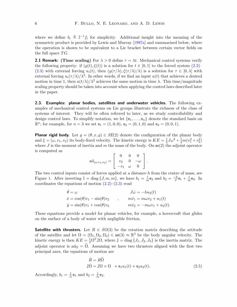
Planar rigid body. Let g = (θ, x, y) ∈ SE(2) denote the configuration of the planar bodyand ξ = (ω, v1, v2) its body-fixed velocity. The kinetic energy is KE = 1

2Jω2 + 1

2m(v21 + v2

2)where J is the moment of inertia and m the mass of the body. On se(2) the adjoint operatoris computed as

ad(ω,v1,v2) =

0 0 0v2 0 −ω−v1 ω 0

.The two control inputs consist of forces applied at a distance h from the centre of mass, seeFigure 1. After inverting I = diag J,m,m, we have b1 = 1

me2 and b2 = −hJ e1 + 1

me3. Incoordinates the equations of motion (2.2)–(2.3) read

θ = ω Jω = −hu2(t)

x = cos(θ)v1 − sin(θ)v2 , mv1 = mωv2 + u1(t)

y = sin(θ)v1 + cos(θ)v2 mv2 = −mωv1 + u2(t).

These equations provide a model for planar vehicles, for example, a hovercraft that glideson the surface of a body of water with negligible friction.

Satellite with thrusters. Let R ∈ SO(3) be the rotation matrix describing the attitudeof the satellite and let Ω = (Ω1,Ω2,Ω3) ∈ so(3) ≈ R3 be the body angular velocity. Thekinetic energy is then KE = 1

2ΩT JΩ, where J = diag J1, J2, J3 is the inertia matrix. The

adjoint operator is adΩ = Ω. Assuming we have two thrusters aligned with the first twoprincipal axes, the equations of motion are

R = RΩ

JΩ = JΩ× Ω + e1u1(t) + e2u2(t). (2.5)

Accordingly, b1 = 1J1e1 and b2 = 1

J2e2.


Σs

g = (θ, x, y)

CMf2

f1

h

Figure 1. Rigid body in SE(2) with two forces applied at a pointa distance h from the centre of mass CM. Σs denotes an inertialreference system. g = (θ, x, y) denotes the position of the body.The body reference frame (not depicted) is aligned with thedirection of application of f1 and f2.

Satellite with rotors. Satellites can alternatively be equipped with internal rotors (mo-mentum wheels). Consider the case in which there are two rotors aligned with two prin-cipal axes of the satellite. The configuration of the satellite plus rotor system is describedby R ∈ SO(3) and (θ1, θ2) ∈ R2 (describing the angular position of the wheels). LetΩrot = (θ1, θ2, 0) denote the angular velocities of the rotors and Ω the angular velocities ofthe carrier. The kinetic energy is

KE =1

2ΩT (Jlock − Jrot)Ω +

1

2(Ω + Ωrot)

T Jrot(Ω + Ωrot),

where Jlock = diag J1, J2, J3 is the inertia of the satellite-rotors system with the rotorslocked, while Jrot = diag(Jrot1, Jrot2, 0) is the inertia of the rotors about their spin axes.From the kinetic energy we compute the inertia matrix as

Jsat-rot =

[Jlock Jrot

Jrot Jrot

].

Also, the adjoint operator satisfies ad(Ω,Ωrot)(v, w) = (Ω× v, 0). The dynamic equations are[Jlock Jrot

Jrot Jrot

] [Ω

Ωrot

]=

[(JlockΩ + JrotΩrot)× Ω

0

]+

[0

e1u1(t) + e2u2(t)

],

and, by inverting the inertia matrix, the input vectors are

b1 = 1Jrot1−J1 e1 + J1

Jrot1(Jrot1−J1)e4

b2 = 1Jrot2−J2 e2 + J2

Jrot2(Jrot2−J2)e5.


Figure 2. Rigid body in SE(3) with three forces applied at a pointa distance h from the centre of mass.

Underwater vehicle in ideal fluid. The motion of a rigid body in incompressible, irrota-tional and inviscid fluid is Hamiltonian with an inertia tensor which includes added massesand inertias, see [Lamb 1932] or the original work of Kirchhoff. Let (R, p) ∈ SE(3) and(Ω, V ) ∈ se(3) denote the configuration and body velocity of the vehicle. The kinematicequations are

R = RΩ

p = RV.

For a neutrally buoyant ellipsoidal body with uniformly distributed mass, the kinetic energyis KE = 1

2ΩT JΩ + 12V

TMV , where the mass and inertia matrices of the body-fluid systemare M = diag m1,m2,m3 and J = diag J1, J2, J3. The adjoint operator is given byequation (2.1). The unforced dynamic equations are therefore

JΩ = JΩ× Ω + MV × VMV = MV × Ω.

Finally, we assume there are three body-fixed forces applied at a point a distance h fromthe centre of mass, as depicted in Figure 2. The corresponding input vectors are

b1 = 1m1

e4, b2 = − hJ3e3 + 1

m2e5, and b3 = h

J2e2 + 1

m3e6.

3. Local controllability properties

This section deals with the nonlinear controllability properties of the systems describedabove. Our treatment was originally presented by Bullo and Lewis [1996]; it is based on


the conditions for small-time local controllability (STLC) by Sussmann [1987] and for con-figuration controllability by Lewis and Murray [1997a]. While our accessibility analysis issimilar to that of Bonnard [1984], Crouch [1984] and Manikonda and Krishnaprasad [1997],important differences in studying controllability include focusing on small-time, local con-trollability properties (as opposed to global controllability) and investigating configurationcontrollability (as opposed to full-state controllability). Configuration controllability con-cerns the reachable set restricted to the configuration space G and is weaker than full-statecontrollability. The controllability conditions presented in this section provide us withenough information to allow control design for low-velocity maneuvers (described in Sec-tion 5). The main limitation is the assumption that the system is initially at rest. Theexamples at the end of this section and the perturbation analysis in the next section provideinsight into these controllability results.

3.1. Definitions and tests. For T > 0, a solution of the system (2.2)–(2.3), is a pair (g, u),where g : [0, T ] → G is a piecewise smooth curve on G, u : [0, T ] → Rm is an admissibleinput in Um and (g(t), u(t)) are a solution to the equations (2.2)–(2.3). Let g0 ∈ G, letV ⊂ G be a neighbourhood of g0 and let W ⊂ G× g be a neighbourhood of (g0, 0g), wherewe let 0g denote the zero vector in g. For T > 0, set

RVG(g0, T ) = g1 ∈ G | there exists a solution (g, u) of the system (2.2)–(2.3)

such that (g, ξ)(0) = (g0, 0g), g(t) ∈ V for t ∈ [0, T ] and g(T ) = g1,

and define the set of reachable configurations as

RVG(g0,≤ T ) =⋃

0≤t≤TRVG(g0, T ).

Similarly, set

RWG×g(g0, T ) = (g1, ξ1) ∈ G×g | there exists a solution (g, u)(t) of the system (2.2)–(2.3)

such that (g, ξ)(0) = (g0, 0g), (g, ξ)(t) ∈W for t ∈ [0, T ] and (g, ξ)(T ) = (g1, ξ1),

and define the set of reachable states as

RWG×g(g0,≤ T ) =⋃

0≤t≤TRWG×g(g0, T ).

Accessibility and configuration accessibility. We present definitions, tools and tests thatcharacterise two notions of accessibility.

3.1 Definition: The system (2.2)–(2.3) is small-time locally accessible at g0 and zerovelocity if RWG×g(g0,≤ T ) contains a non-empty open subset of G× g for all T > 0 and forall neighbourhoods W of (g0, 0g). If this holds for any g0 ∈ G, then the system is calledsmall-time locally accessible at zero velocity (accessible at zero velocity).

The system (2.2)–(2.3) is small-time locally configuration accessible at g0 ifRVG(g0,≤ T ) contains a non-empty open subset of G for all T > 0 and for all neigh-bourhoods V of g0. If this holds for each g0 ∈ G, then the system is called small-timelocally configuration accessible (configuration accessible).


The following concepts are helpful in providing computable tests for the notions of ac-cessibility. Let us denote with B = b1, . . . , bm the family2 of input vectors. Recall thatthe involutive closure of B, denoted by Lie(B), is the set of vectors obtained by takingiterated Lie brackets of the vectors b1, . . . , bm. Additionally, we define the symmet-ric closure of B, denoted by Sym(B), as the set of vectors obtained by taking iteratedsymmetric products of the vectors b1, . . . , bm.3.2 Proposition: Consider the system (2.2)–(2.3) and let B = b1, . . . , bm be the family ofinput vectors.

1. The system is locally accessible at zero velocity if and only if the subspace defined bySym(B) has full rank.

2. The system is locally configuration accessible if and only if the subspace defined byLie(Sym(B)) has full rank.

These results are a direct consequence of the accessibility computations of Lewis and Murray[1997a].

Controllability and configuration controllability. Next we present two corresponding no-tions of controllability: the “classic” small-time local controllability and a weaker versioncalled small-time local configuration controllability.

3.3 Definition: The system (2.2)–(2.3) is small-time locally controllable at g0 and atzero velocity if RWG×g(g0,≤ T ) contains a non-empty open subset of G × g for all T > 0and for all neighbourhoods W of (g0, 0g), and (g0, 0g) belongs to the interior of this subset.If this holds for any g0 ∈ G, then the system is called small-time locally controllable atzero velocity (STLC at zero velocity).

The system (2.2)–(2.3) is small-time locally configuration controllable at g0 ifRVG(g0,≤ T ) contains a non-empty open subset of G for all T > 0 and for all neighbourhoodsV of g0, and g0 belongs to the interior of this subset. If this holds for each g0 ∈ G, thenthe system is called small-time locally configuration controllable (STLCC).

To establish tests that distinguish controllability from accessibility, we need to introducethe notions of good and bad symmetric products and order of a symmetric product. Herewe do this in a somewhat simplified way to avoid introducing too much mathematicalmachinery (i.e., the notion of free Lie algebras of indeterminates).

The order of an iterated symmetric product of factors from Sym(B) is the total numberof factors. We say that a symmetric product from Sym(B) is bad if it contains an evennumber of each of the vectors in B. Otherwise, we say that the symmetric product is good .For example, the symmetric product 〈〈b1 : b2〉 : b1〉 has order three and it is good, thesymmetric product 〈〈〈b1 : b2〉 : b2〉 : b1〉 has order four and it is bad. More instances of goodand bad symmetric products can be found in the next section.

3.4 Proposition: Consider the system (2.2)–(2.3) and let B = b1, . . . , bm be the family ofinput vectors.

2Equivalently, we can think of B as a linear subspace of g or a left-invariant distribution on G.


1. The system is STLC at zero velocity if the subspace defined by Sym(B) has full rankand every bad symmetric product is a linear combination of lower-order good symmet-ric products.

2. The system is STLCC if the subspace defined by Lie(Sym(B)) has full rank and everybad symmetric product is a linear combination of lower-order good symmetric products.

These results are a direct consequence of the results of Sussmann [1987] and Lewisand Murray [1997a]. We note that symmetric and involutive closures are simple algebraicoperations that characterise controllability for the (strongly) nonlinear system (2.2)–(2.3),independent of the base point g0 ∈ G. These tests have a simple interpretation; symmetricproducts of input vectors identify which velocities are reachable, whereas Lie brackets ofreachable velocities identify which configurations are reachable. The only restriction weimpose is the requirement that the system be initially at rest.

Note that the distinction between good and bad symmetric products is analogous tothe notion of good and bad Lie brackets in [Sussmann 1987]. Similar characterisations areusually introduced when dealing with controllability properties for systems with drift. Inthe next section we present some approximate solutions that give some insight into therequirement that “bad products are spanned by lower-order good products.”

Single-input systems (n > m = 1) always fail the sufficient condition for both controlla-bility notions; if only one input vector is available, the only possible nontrivial second-ordersymmetric product is bad. It can further be proven that single-input systems are neitherSTLC at zero velocity nor STLCC, see [Lewis 1997].

3.2. Applications to the examples. We investigate the controllability properties of thesystems introduced in Section 2.3. Our examples are selected to be instructive.

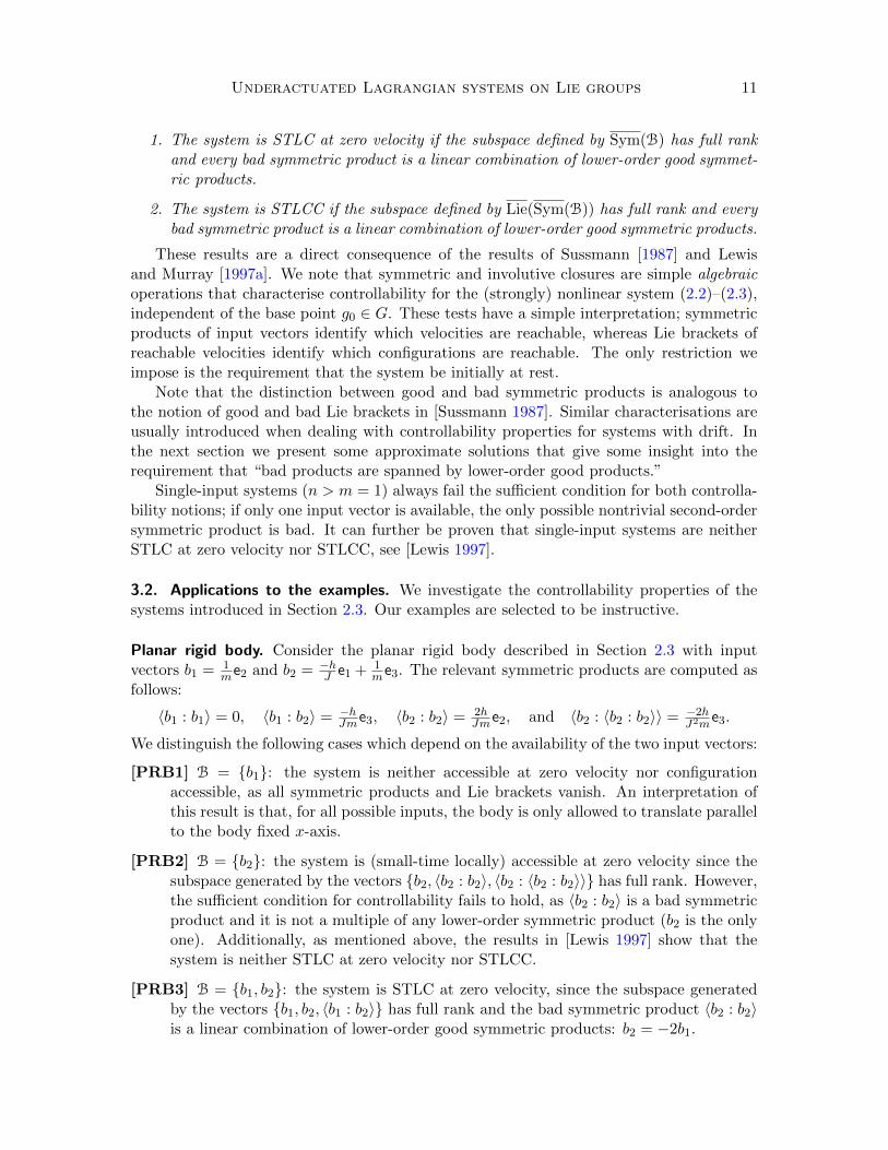
Planar rigid body. Consider the planar rigid body described in Section 2.3 with inputvectors b1 = 1

me2 and b2 = −hJ e1 + 1

me3. The relevant symmetric products are computed asfollows:

〈b1 : b1〉 = 0, 〈b1 : b2〉 = −hJme3, 〈b2 : b2〉 = 2h

Jme2, and 〈b2 : 〈b2 : b2〉〉 = −2hJ2m

e3.

We distinguish the following cases which depend on the availability of the two input vectors:

[PRB1] B = b1: the system is neither accessible at zero velocity nor configurationaccessible, as all symmetric products and Lie brackets vanish. An interpretation ofthis result is that, for all possible inputs, the body is only allowed to translate parallelto the body fixed x-axis.

[PRB2] B = b2: the system is (small-time locally) accessible at zero velocity since thesubspace generated by the vectors b2, 〈b2 : b2〉, 〈b2 : 〈b2 : b2〉〉 has full rank. However,the sufficient condition for controllability fails to hold, as 〈b2 : b2〉 is a bad symmetricproduct and it is not a multiple of any lower-order symmetric product (b2 is the onlyone). Additionally, as mentioned above, the results in [Lewis 1997] show that thesystem is neither STLC at zero velocity nor STLCC.

[PRB3] B = b1, b2: the system is STLC at zero velocity, since the subspace generatedby the vectors b1, b2, 〈b1 : b2〉 has full rank and the bad symmetric product 〈b2 : b2〉is a linear combination of lower-order good symmetric products: b2 = −2b1.


Satellite with thrusters. Consider the satellite with thrusters described in Section 2.3.Input vectors are b1 = 1

J1e1 and b2 = 1

J2e2. The relevant symmetric products and Lie

brackets are computed as

〈b1 : b1〉 = 〈b2 : b2〉 = 0, 〈b1 : b2〉 = J2−J1J1J2J3

e3, and [b1, b2] = 1J1J2

e3.

The controllability properties are as follows:

[ST] B = b1, b2 and J1 6= J2: if the satellite is not axisymmetric3, then the rank ofb1, b2, 〈b1 : b2〉 is full and there are no bad symmetric products. Therefore, thesystem is STLC at zero velocity.

Satellite with rotors. Consider the satellite with rotors introduced in Section 2.3. For b1and b2 defined in Section 2.3, we compute symmetric products and Lie brackets as

〈b1 : b1〉 = 〈b2 : b2〉 = 〈b1 : b2〉 = 0,

and

[b1, b2] = 1(Jrot1−J1)(Jrot2−J2)e3,

[[b1, b2] , b1] = 1(Jrot1−J1)2(J2−Jrot2)

e2,

[[b1, b2] , b2] = 1(Jrot1−J1)(Jrot2−J2)2

e1.

[SR] B = b1, b2: the system is not accessible at zero velocity (every symmetric productvanishes) and hence not STLC, but it is STLCC since the involutive closure has fullrank.

This result was partly expected but not trivial. Since the satellite-rotors system is notsubject to any external force, its total angular momentum is conserved. Therefore, it isintuitively clear that the system cannot be accessible in both configurations and velocities.However, the less trivial fact is that the system is STLCC. This means that, despite theconservation law, any configuration can be reached, that is, any orientation R together withany rotor angles (θ1, θ2).

Underwater vehicle in ideal fluid. Consider the underwater vehicle introduced in Sec-tion 2.3, with the input forces depicted in Figure 2. We compute some good symmetricproducts as

〈b1 : b2〉 = m2−m1J3m1m2

e3 − hJ3m2

e5,

〈b1 : b3〉 = m1−m3J2m1m3

e2 − hJ2m3

e6,

〈b2 : b3〉 = 1J1

(h2

J3− h2

J2− 1

m3+ 1

m2

)e1

and some bad ones as

〈b1 : b1〉 = 0, 〈b2 : b2〉 = 2hI3m1

e4, 〈b3 : b3〉 = 2hI2m1

e4.

3If the satellite is axisymmetric, i.e., J1 = J2, then a simple analysis shows that the system is STLCC.


[UV] B = b1, b2, b3: Consider the 6×6 matrix defined by the good symmetric products oforder one and two, that is b1, b2, b3, 〈b1 : b2〉, 〈b1 : b3〉, 〈b2 : b3〉. This matrix is gener-ically nonsingular.4 Hence, the system is small-time locally accessible at zero velocity.Additionally, since the bad second-order symmetric products are proportional to b1,they are spanned by good lower-order symmetric products (b1 is a good symmetricproduct of order 1). Therefore, the system is generically STLC at zero velocity.

4. Approximate solutions under small-amplitude forcing

In this section we investigate the behaviour of system (2.2)–(2.3) under small-amplitudeforcing. The key analysis tool is the standard perturbation method as described by Khalil[2001]. Assuming a small-amplitude input (say of order ε, for 0 < ε << 1), this methodprovides us with a solution to system (2.2)–(2.3) in the form of a Taylor series in ε. Sincethe computation of only a few terms in the series is tractable, we obtain an approximateexpansion. However, this estimate illustrates the role of symmetric products and Lie brack-ets in determining the solution of the forced system (2.2)–(2.3). Therefore, this estimateprovides insight into the controllability tests introduced above and, as we shall see, it isinstrumental in designing the motion algorithms of the next section.

4.1. Notation and results. We introduce the following notation. Given a possibly vector-valued function h(t) with t ∈ R+, define its first integral function h(t) with t ∈ R+, as thefinite integral from 0 to t

h(t) ,∫ t

0h(τ)dτ.

Higher-order integrals, as for example h(t) are defined recursively. In the following, weconsider inputs of the form

ui(t, ε) = εu1i (t) + ε2u2

i (t)

where 0 < ε << 1 and where u1i , u

2i are O(1). Accordingly, we write the resultant forcing∑

i biui(t, ε) as the sum of two terms of different order in ε

m∑i=1

biui(t, ε) =

m∑i=1

bi(εu1i (t) + ε2u2

i (t))

= ε b1(t) + ε2 b2(t), (4.1)

where we define b1(t) =∑m

i=1 biu1i (t) and b2(t) =

∑mi=1 biu

2i (t). In the following, given any

quantity y(ε), we let yk denote the kth term in the Taylor expansion of y(ε) about ε = 0; forexample, we will write ξ(t, ε) = εξ1(t)+ε2ξ2(t)+O(ε3). The following proposition describesthe system’s behaviour when forced by small (order ε and order ε2) amplitude inputs asdefined in equation (4.1).

4The matrix is singular when h2m1m2 + J3(m1 −m2) = 0 or when h2m1m3 + J2(m1 −m3) = 0or when h2(1/J3 − 1/J2) = 1/m3 − 1/m2.


4.1 Proposition: (Approximate evolution) For 0 < ε << 1 and for inputs of the formin equation (4.1), let (g(t), ξ(t)) be the solutions of system (2.2)–(2.3). Let x(t) be theexponential coordinates of g(t) about the initial condition g(0) = Id. Also, write the initialvelocity as ξ(0) = εξ1

0 + ε2ξ20 where ξ1

0 and ξ20 are O(1).

Then for t ∈ [0, 2π] it holds that ξ(t, ε) = εξ1(t) + ε2ξ2(t) + ε3ξ3(t) +O(ε4), with

ξ1(t) = ξ10 + b1(t),

ξ2(t) = ξ20 − 〈ξ1

0 : ξ10〉t

2− 〈ξ1

0 : b1(t)〉+(b2 − 1

2〈b1 : b1〉)

(t),

ξ3(t) = −〈ξ10 : ξ2

0〉t+ 〈ξ10 : 〈ξ1

0 : ξ10〉〉

t2

4+ 〈ξ1

0 : 〈ξ10 : b1(t)〉〉 − 〈ξ1

0 :

(b2 − 1

2〈b1 : b1〉)

(t)〉

− 〈b1(t) : ξ20〉+ 1

2〈〈ξ10 : ξ1

0〉t : b1(t)〉+ 〈b1 : 〈ξ10 : b1〉〉(t)− 〈b1 :

(b2 − 1

2〈b1 : b1〉)〉(t),

and x(t, ε) = εx1(t) + ε2x2(t) +O(ε3), with

x1(t) = ξ10t+ b1(t),

x2(t) = ξ20t− 〈ξ1

0 : ξ10〉t2

4+

(b2 − 1

2〈b1 : b1〉)

(t)− 〈ξ10 : b1(t)〉+ 1

2

[ξ1

0 + b1, ξ10t+ b1

](t).

The proof is based on the standard perturbation method as described by Khalil [2001] andon the approximate solutions for the kinematic system obtained by Fomenko and Chakon[1990]; see Appendix A.1 for a detailed account. Note that both symmetric products andLie brackets show up in the Taylor expansions and this agrees with the controllability testspresented above. Also, note that the approximations in Proposition 4.1 hold only over afinite period of time and particular care is needed in order to compute approximations validover a time interval of order 1/ε.

4.2. Application to examples. We now relate the approximations above to the controlla-bility tests of the previous section. To simplify the expansions above and to investigate thenonlinear second-order effects of the inputs, we let the initial velocity vanish, ξ(0) = 0g,

and the first order input b1(t) verify b1(2π) = b1(2π) = 0g. It holds that

ξ(2π) ≈ ε2(b2 − 1

2〈b1 : b1〉)

(2π), and x(2π) ≈ ε2(b2 − 1

2〈b1 : b1〉+ 12

[b1, b1

])(2π),

(4.2)where, for the remainder of this section, the symbol ≈ denotes an equality up to a thirdorder error in ε. Also, if we set b2(t) = 0g, it holds that

ξ(2π) ≈ −12ε

2〈b1 : b1〉(2π), and x(2π) ≈ −12ε

2

(〈b1 : b1〉+

[b1, b1

])(2π). (4.3)

Up to a higher-order error in ε, the final velocity ξ(2π) is determined by certain symmet-ric products and the final configuration variable x(2π) is determined by certain symmetricproducts and Lie brackets. Next, we study in more detail these remaining terms to gainsome insight into what terms are “good,” what are “bad” and which ones we can exploitto design motion algorithms.


CM

e2e3

fresultant = ±ǫ(sin(t)− 2 sin(2t))f2

Figure 3. Planar rigid body with single forcing [PRB2]. Witha resultant external force ±ε cos(t) and after a period 2π,the approximate final reconfiguration is log(g(0)−1g(2π)) =−2πε2 h

Jme2 and the approximate final velocity is ξ(2π) =

−2π2ε2 hJme2.

Single-input systems: relative equilibria and bad symmetric products. Both examples ofplanar rigid bodies, [PRB1] and [PRB2], are single-input systems. Recall that [PRB1]denotes the system with a single force b1 with the line of action through the centre of mass,and [PRB2] denotes the system with the single force b2 applied at a point a distance hfrom the centre of mass and perpendicular to b1, see Figure 1.

Let bsi denote the single input vector, e.g., bsi = b1 in [PRB1] and bsi = b2 in [PRB2].If the symmetric product 〈bsi : bsi〉 vanishes, see the [PRB1] example, the system is neitheraccessible nor configuration accessibility, and the final state (x, ξ)(2π) vanishes. Recall fromSection 2, that for any vector η such that 〈η : η〉 ≡ ad∗η Iη = 0, the curve t ∈ R 7→ (exp(tη), η)is a relative equilibria, i.e., a motion corresponding to constant body-fixed velocity. Thus,an actuator bsi aligned with a relative equilibria has vanishing bad symmetric product〈bsi : bsi〉.

Also instructive is the case in which the bad symmetric product 〈bsi : bsi〉 does not vanish,

e.g., the [PRB2] system. Assuming b1(t) = bsiφ(t) and φ(2π) = φ(2π) = 0, equations (4.3)lead to

ξ(2π) ≈ −12ε

2

∫ 2π

0φ

2dt 〈bsi : bsi〉, and x(2π) ≈ −1

2ε2

∫ 2π

0

∫ s

0φ

2dsdt 〈bsi : bsi〉. (4.4)

As already mentioned, configuration and velocity change an amount proportional to ε2

along the direction 〈bsi : bsi〉. Additionally, notice that it is impossible to change the signof the motion, which will always be along −〈bsi : bsi〉. For example the [PRB2] systemwith forcing amplitude ±ε cos(t), always moves in the direction −e2, i.e., to the left (seeFigure 3). This phenomenon suggests that the system is not locally controllable, as certainconfigurations appear to be not reachable. However, equation (4.4) does not prove thisclaim as it only specifies the final value x(2π). The sharper analysis by Lewis [1997] isneeded to show that single-input systems are neither STLC at zero velocity nor STLCC.


Multi-input systems with no bad symmetric products. Next we examine systems with(at least) two input forces. We focus on an example with two input vectors b1 and b2 thathave vanishing bad symmetric products 〈b1 : b1〉 = 〈b2 : b2〉 = 0 and either non-zero goodsymmetric product 〈b1 : b2〉 6= 0 or non-zero Lie bracket [b1, b2] 6= 0. The satellite withtwo thrusters [ST] and the satellite with two rotors [SR] are such examples. Pluggingb1(t) = b1u1(t) + b2u2(t) into equations (4.3), we have

ξ(2π) ≈ −12ε

2〈u1b1 + u2b2 : u1b1 + u2b2〉(2π)

= −ε2〈b1 : b2〉u1 u2(2π)

and

x(2π) ≈ −12ε

2

(〈b1 : b1〉+

[b1, b1

])(2π)

= −ε2〈b1 : b2〉u1 u2(2π)− ε2 [b1, b2]u1 u2 − u1 u2(2π).

We interpret the operations performed on the input signals u1(t) and u2(t) as follows:u1 u2(2π) is the inner product in the L2[0, 2π] function space between u1(t) and u2(t),

whereas u1 u2 − u1 u2(2π) is the area enclosed by the plot of signals u1(t) versus u2(t). Wedistinguish two cases:

• Out-of-phase sinusoidal inputs generate motion along Lie brackets: First, considerthe satellite with rotors [SR] example that is STLCC but not STLC at zero velocity.The symmetric product 〈b1 : b2〉 vanishes, so that we have from equation (4.3)

ξ(2π) ≈ 0 and x(2π) ≈ −ε2 [b1, b2]u1 u2 − u1 u2(2π).

If we want to steer the configuration x(2π) in the direction [b1, b2], sinusoidal signalsat the same frequency and out-of-phase are a simple standard choice. This is one ofthe basic ideas behind the algorithms presented by Leonard and Krishnaprasad [1995]and other literature on motion planning for driftless control systems.

• In-phase sinusoidal inputs generate motion along good symmetric products: Second,consider the satellite with thrusters example [ST] that is STLC at zero velocity sincethe symmetric product 〈b1 : b2〉 6= 0. If we pick sinusoidal inputs at the same frequencyand in-phase, e.g., u1(t) = u2(t) = cos(t), the contribution proportional to the Liebracket [b1, b2] vanishes, since the area included by two identical signal is zero. Further,it holds that

ξ(2π) ≈ −ε2〈b1 : b2〉(u1)2(2π) and x(2π) ≈ −ε2〈b1 : b2〉(u1)2(2π),

and both velocity and configuration variables vary along −〈b1 : b2〉.5 Motion in thesymmetric product direction is generated with sinusoidal inputs at the same frequencyand in-phase. This is in contrast with the previous case and it is reminiscent of someresults on gait selection for locomotion systems with drift, see the 1:1 gait in [Ostrowskiand Burdick 1997].

5Also, the velocity change is maximal in the sense that on the L2[0, 2π] function space the Cauchy-Schwartz inequality on the inner product of u1(t) and u2(t) holds with equality if u1(t) = u2(t).


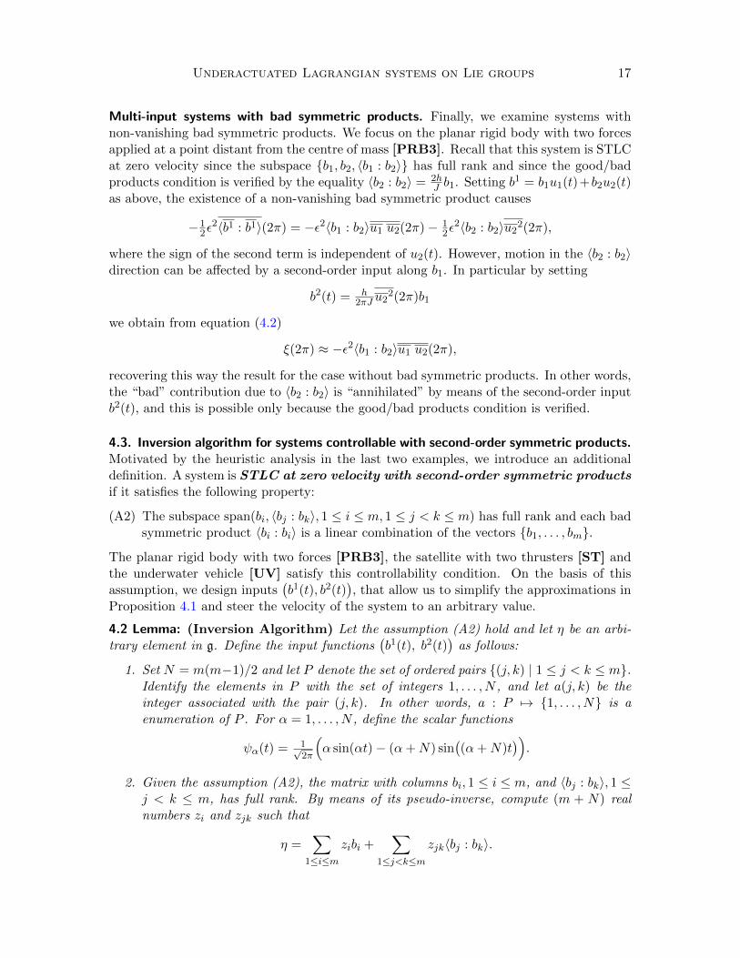
Multi-input systems with bad symmetric products. Finally, we examine systems withnon-vanishing bad symmetric products. We focus on the planar rigid body with two forcesapplied at a point distant from the centre of mass [PRB3]. Recall that this system is STLCat zero velocity since the subspace b1, b2, 〈b1 : b2〉 has full rank and since the good/badproducts condition is verified by the equality 〈b2 : b2〉 = 2h

J b1. Setting b1 = b1u1(t)+b2u2(t)as above, the existence of a non-vanishing bad symmetric product causes

−12ε

2〈b1 : b1〉(2π) = −ε2〈b1 : b2〉u1 u2(2π)− 12ε

2〈b2 : b2〉u22(2π),

where the sign of the second term is independent of u2(t). However, motion in the 〈b2 : b2〉direction can be affected by a second-order input along b1. In particular by setting

b2(t) = h2πJ u2

2(2π)b1

we obtain from equation (4.2)

ξ(2π) ≈ −ε2〈b1 : b2〉u1 u2(2π),

recovering this way the result for the case without bad symmetric products. In other words,the “bad” contribution due to 〈b2 : b2〉 is “annihilated” by means of the second-order inputb2(t), and this is possible only because the good/bad products condition is verified.

4.3. Inversion algorithm for systems controllable with second-order symmetric products.Motivated by the heuristic analysis in the last two examples, we introduce an additionaldefinition. A system is STLC at zero velocity with second-order symmetric productsif it satisfies the following property:

(A2) The subspace span(bi, 〈bj : bk〉, 1 ≤ i ≤ m, 1 ≤ j < k ≤ m) has full rank and each badsymmetric product 〈bi : bi〉 is a linear combination of the vectors b1, . . . , bm.

The planar rigid body with two forces [PRB3], the satellite with two thrusters [ST] andthe underwater vehicle [UV] satisfy this controllability condition. On the basis of thisassumption, we design inputs

(b1(t), b2(t)

), that allow us to simplify the approximations in

Proposition 4.1 and steer the velocity of the system to an arbitrary value.

4.2 Lemma: (Inversion Algorithm) Let the assumption (A2) hold and let η be an arbi-trary element in g. Define the input functions

(b1(t), b2(t)

)as follows:

1. Set N = m(m−1)/2 and let P denote the set of ordered pairs (j, k) | 1 ≤ j < k ≤ m.Identify the elements in P with the set of integers 1, . . . , N , and let a(j, k) be theinteger associated with the pair (j, k). In other words, a : P 7→ 1, . . . , N is aenumeration of P . For α = 1, . . . , N , define the scalar functions

ψα(t) = 1√2π

(α sin(αt)− (α+N) sin

((α+N)t

)).

2. Given the assumption (A2), the matrix with columns bi, 1 ≤ i ≤ m, and 〈bj : bk〉, 1 ≤j < k ≤ m, has full rank. By means of its pseudo-inverse, compute (m + N) realnumbers zi and zjk such that

η =∑

1≤i≤mzibi +

∑1≤j<k≤m

zjk〈bj : bk〉.


3. Finally, set

b1(t) =∑

1≤j<k≤m

√|zjk|

(bj − sign (zjk)bk

)ψa(j,k)(t), (4.5)

b2(t) ≡ b2 =1

2π

∑1≤i≤m

zibi +1

4π

∑1≤j<k≤m

|zjk|(〈bj : bj〉+ 〈bk : bk〉

). (4.6)

The input functions (b1(t), b2(t)) designed in equation (4.5) and (4.6) verify(b2 − 1

2〈b1 : b1〉)

(2π) = η. (4.7)

Appendix A.2 contains the lemma’s proof. In what follows, we denote the procedure de-scribed in the inversion algorithm with the notation:(

b1(t), b2(t))

= Inverse(η) .

A direct manipulation of equation (4.5) and of b1(t) =∑m

i=1 biu1i (t) leads to the equiv-

alent statement

u1i (t) = −

i−1∑j=1

√|zji| sign(zji)ψa(j,i)(t) +

m∑j=i+1

√|zij |ψa(i,j)(t).

Note that motion along the good symmetric product direction 〈bi : bj〉 (for i < j) isgenerated by the term

√|zij |ψa(i,j)(t) in u1

i (t) and the term −√|zij | sign(zij)ψa(i,j)(t) in

u1j (t). Hence the inputs u1

i (t) and u1j (t) have the common factor ψa(i,j). The other terms in

the definition of u1k(t) for all k, are at different frequencies. Therefore, they are orthogonal

to ψa(i,j) in the inner product space L2[0, 2π], and so do not generate motion in any othersymmetric product direction. The second term in the second order input b2 compensates forthe motion excited along bad symmetric product directions. Its presence is a key differencewith respect to the algorithms in [Leonard and Krishnaprasad 1995] for driftless systems.

One of the drawbacks of the previous algorithm is that the input functions containrelatively high frequencies, e.g., in an m = 3 input system, the input functions containsinusoids with frequency from 1 to m(m− 1) = 6. This can be mitigated by optimising thedesign of the coefficients zi, zjk and the numbering of the set P . For example, the designof the coefficients can be optimised by employing a weighted pseudo-inverse.

5. Control algorithms from motion primitives

In this section we design motion control algorithms based on the approximations inProposition 4.1 and the inversion algorithm in Lemma 4.2. Condition (A1) on the groupG, and condition (A2) on the controllability of the system are assumed. We start bydesigning two primitive motion patterns, Maintain-Velocity and Change-Velocity, thatprovide the system with some basic motion capabilities. We then focus on more complexcontrol algorithms to solve the point-to-point reconfiguration problem, the local exponentialstabilisation problem and the static interpolation problem.


5.1. Primitives of motion. We describe two basic maneuvers that each last 2π units oftime. The parameter σ 1 is a small positive constant. To maintain a velocity of orderO(σ), an input of order O(σ) suffices, while to obtain a change in velocity of order O(σ),we employ a control input of order O(

√σ). Each primitive is described in terms of initial

configuration and velocity, input design, and final configuration and velocity.

Maintain-Velocity(σ, ξref): keeps the body velocity ξ(t) close to a reference value σξref.

Initial state:g(0) = g0,ξ(0) = σξref + σ2ξerror,

Input:ε= σ,

(b1, b2) = Inverse(π〈ξref : ξref〉 − ξerror),

Final state:log(g−1

0 g(2π)) = 2πσξref + πσ2ξerror +O(σ3),ξ(2π) = σξref +O(σ3).

Change-Velocity(σ, ξfinal): steer the body velocity ξ(t) to a final value σξfinal.

Initial state:g(0) = g0,ξ(0) = σξ0,

Inputε=√σ,

(b1, b2) = Inverse(ξfinal − ξ0),

Final state:log(g−1

0 g(2π)) = πσ(ξ0 + ξfinal) +O(σ3/2),ξ(2π) = σξfinal +O(σ2).

The statements on the final configuration and velocity of the primitives are proved inAppendix A.3. Note that the magnitude of control input is

‖π〈ξref : ξref〉 − ξerror‖O(σ), during a Maintain-Velocity(σ, ξref) primitive,

‖ξfinal − ξ0‖O(√σ), during a Change-Velocity(σ, ξfinal) primitive.

We conclude this section by showing how to compute estimates of final configurations af-ter multiple periods of control. The following result is a direct consequence of the Campbell-Baker-Hausdorff formula, see for example [Sattinger and Weaver 1986].

5.1 Lemma: Let σ 1 be a positive constant and let g0, g1 be group elements. Define theexponential coordinates y0 = log(g0) ∈ g and y1 = log(g1) ∈ g. If the vector [y0, y1] is higherorder in σ than (y0 + y1), then it holds

log(g0g1) = y0 + y1 +O([y0, y1]).

5.2. Control algorithms. We present three algorithms to solve various motion controlproblems. These algorithms combine the two motion primitives with a discrete-time feed-back. This makes the approximations hold over multiple time intervals; for example, overa time interval of order 1/σ.

Point-to-point reconfiguration problem. This motion task reconfigures the system, i.e.,changes its position and orientation, starting and ending at zero velocity. We assume thatthe initial state is (g(0), ξ(0)) = (g0, 0g) and the final desired state is (g1, 0g). For simplicity,


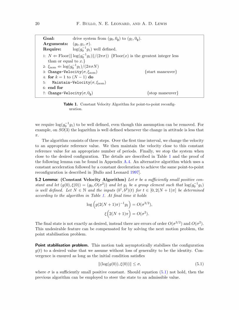
Goal: drive system from (g0, 0g) to (g1, 0g).Arguments: (g0, g1, σ).

Require: log(g−10 g1) well defined.

1: N ⇐ Floor(‖ log(g−10 g1)‖/(2πσ)) Floor(x) is the greatest integer less

than or equal to x.2: ξnom ⇐ log(g−1

0 g1)/(2πσN)3: Change-Velocity(σ, ξnom) start maneuver4: for k = 1 to (N − 1) do5: Maintain-Velocity(σ, ξnom)6: end for7: Change-Velocity(σ, 0g) stop maneuver

Table 1. Constant Velocity Algorithm for point-to-point reconfig-uration.

we require log(g−10 g1) to be well defined, even though this assumption can be removed. For

example, on SO(3) the logarithm is well defined whenever the change in attitude is less thatπ.

The algorithm consists of three steps. Over the first time interval, we change the velocityto an appropriate reference value. We then maintain the velocity close to this constantreference value for an appropriate number of periods. Finally, we stop the system whenclose to the desired configuration. The details are described in Table 1 and the proof ofthe following lemma can be found in Appendix A.4. An alternative algorithm which uses aconstant acceleration followed by a constant deceleration to achieve the same point-to-pointreconfiguration is described in [Bullo and Leonard 1997].

5.2 Lemma: (Constant Velocity Algorithm) Let σ be a sufficiently small positive con-stant and let (g(0), ξ(0)) = (g0, O(σ2)) and let g1 be a group element such that log(g−1

0 g1)is well defined. Let N ∈ N and the inputs (b1, b2)(t) for t ∈ [0, 2(N + 1)π] be determinedaccording to the algorithm in Table 1. At final time it holds

log(g(2(N + 1)π)−1g1

)= O(σ3/2),

ξ(

2(N + 1)π)

= O(σ2).

The final state is not exactly as desired, instead there are errors of order O(σ3/2) and O(σ2).This undesirable feature can be compensated for by solving the next motion problem, thepoint stabilisation problem.

Point stabilisation problem. This motion task asymptotically stabilises the configurationg(t) to a desired value that we assume without loss of generality to be the identity. Con-vergence is ensured as long as the initial condition satisfies

‖(log(g(0)), ξ(0))‖ ≤ σ, (5.1)

where σ is a sufficiently small positive constant. Should equation (5.1) not hold, then theprevious algorithm can be employed to steer the state to an admissible value.


Goal: drive system to the state (Id, 0g) exponentially as t→∞.Arguments: σ.Require: ‖(log(g(0)), ξ(0))‖ ≤ σ.

1: for k = 1 to +∞ do2: tk ⇐ 4kπ tk is the current time3: σk ⇐ ‖(log(g(tk), ξ(tk)))‖4: Change-Velocity

(σk,−

(log(g(tk)) + πξ(tk)

)/(2πσk)

)5: Change-Velocity(σk, 0g)6: end for

Table 2. Local Exponential Stabilisation Algorithm.

The key idea of the algorithm is to iterate the following procedure: measure the stateat time tk and design control inputs that try to steer the state to the desired value (Id, 0g)at time tk+1 = tk + 4π. Since we impose two requirements, one on the final configurationand one on the final velocity, two calls to the Change-Velocity primitive are needed. Theidea of iterating an approximate stabilisation step for fast convergence can be found, forexample, in [Lafferriere and Sussmann 1991]. The details are described in Table 2 and theproof of the following lemma is in Appendix A.5.

5.3 Lemma: (Local Exponential Stabilisation Algorithm) Let σ be a sufficientlysmall positive constant and assume the initial condition satisfies equation (5.1). Let theinputs (b1(t), b2(t)) be determined according to the algorithm in Table 2 and let tk = 4kπ.Then there exists a λ > 0 such that∥∥( log(g(tk)), ξ(tk)

)∥∥ ≤ ∥∥( log(g(0)), ξ(0))∥∥ e−λtk , ∀ k ∈ N.

Additionally, for t ∈ [4kπ, 4(k + 1)π] it holds that∥∥( log(g(t), ξ(t)

)∥∥ = O(e−λk/2).

Static interpolation problem. This motion task steers the system’s configuration alonga path connecting the set of the ordered points g0, g1, . . . , gM. As above, we requirelog(g−1

k−1gk) to be well defined for 1 ≤ k ≤ M . The algorithm consists of M repeatedconstant velocity (point-to-point) maneuvers (Table 1), with the only difference being thatwhen the configuration reaches the the kth desired value gk, the velocity gets changeddirectly to the reference value for the next interval, i.e., without stopping. The details aredescribed in Table 3. It can be shown that the configuration g(t) follows a path passingthrough the points g0, g1, . . . , gM with an error of order σ. We do not include a full proofof convergence as it is very similar to the one for Lemma 5.2.

5.4 Remark: (Interpolating sequences of relative equilibria versus constant veloc-ity motions) The Constant Velocity and the Static Interpolation Algorithms provide twodifferent solutions to the reconfiguration problem. These two algorithms can be comparedon the basis of an input cost of the form

‖u‖[0,T ] =

∫ T

0L(u(t))dt,


Goal: drive system through points g0, g1, . . . , gM.Arguments: (g0, g1, . . . , gM , σ).

Require: (g(0), ξ(0)) = (g0, 0g) and log(g−1i gi) well defined for all 0 ≤ i ≤M .

1: for j = 1 to M do2: gtmp,j ⇐ g(t) exp(πξ(t)) t is the current time3: Nj ⇐ Floor(‖ log(g−1

tmp,jgj)‖/(2πσ))

4: ξnom,j ⇐ log(g−1tmp,jgj)/(2πσNj)

5: Change-Velocity(σ, ξnom,j)6: for k = 1 to (Nj − 1) do7: Maintain-Velocity(σ, ξnom,j)8: end for9: end for

10: Change-Velocity(σ, 0g)

Table 3. Static Interpolation Algorithm.

where T = T (σ) is the time required to complete the maneuver and L : Um 7→ R is acost on the space of input functions. In the following we let gi and gf denote initial andfinal (desired) configurations and we let P = g0 = gi, g1, . . . , gM = gf be a sequence ofconfigurations such that log(g−1

j−1gj) is a relative equilibrium vector for all j = 1, . . . ,M .Recall that η ∈ g is a relative equilibrium vector if 〈η : η〉 vanishes.

1. The Constant Velocity Algorithm to go from g0 to gf involves 2 calls to theChange-Velocity primitive and (N − 1) calls to the Maintain-Velocity primitive.Using notation from Table 1 and some of the details in Appendix A.4, the cost of thecomplete maneuver can be computed as

‖u‖[0,T ] = 2O(√σ) + (N − 1)‖〈ξnom : ξnom〉‖O(σ) = O(1),

since ‖〈ξnom : ξnom〉‖ is of order 1 and N is of order 1/σ.

2. The Static Interpolation Algorithm applied to the set of configurations P in-volves (M + 2) calls to the Change-Velocity primitive and (

∑Mj=1Nj) calls to the

Maintain-Velocity primitive. With the notation in Table 3, a little algebra showsthat

‖u‖[0,T ] = (M + 2)O(√σ) + (

∑jNj)‖〈ξnom,j : ξnom,j〉‖O(σ).

Since the configuration g(t) follows the path determined by the set P with an error oforder σ, and since log(g−1

j−1gj) is a relative equilibrium vector, it can be shown that〈ξnom,j : ξnom,j〉 = O(σ). Summarising, the total cost is

‖u‖[0,T ] = (M + 2)O(√σ) + (

∑jNj)O(σ2) = O(

√σ).

We conclude that for small σ (or equivalently, for long final times T = O(1/σ)), movingalong a set of relative equilibria is a more efficient strategy than the Constant VelocityAlgorithm. In other words, planning a path along relative equilibria takes into takes intoproper account the full system’s dynamics and leads to some notion of optimality.


Figure 4. Constant Velocity Algorithm. The bullet-shaped ob-jects drawn in the left picture represent the location of theplanar body. Darker objects correspond to the location of thebody at the beginning and end of a primitive. The plots on theright display the time-evolution of variables (u1, u2, ω, v1, v2).

5.3. Numerical simulations. The three algorithms introduced above have been imple-mented on a planar rigid body with two forces a distance h from the centre of mass andwith two different masses along the body-fixed axes (to account for added mass when thebody is in a fluid). This example is very similar to [PRB3] of Section 2.3. The parametervalues in normalised units were chosen to be J = 1,m1 = .6,m2 = 1, h = 2. For boththe Constant Velocity Algorithm and the Static Interpolation Algorithm, we let the initialconfiguration be the identity and the final (desired) configuration consist of a rotation ofπ and a translation of 2 units along the y-axis, i.e., ginitial = (0, 0, 0) and gfinal = (π, 0, 2).We set σ = .1. For all three algorithms, the numerical results were in agreement with thetheoretical analysis presented above.

Constant Velocity, Table 1: Figure 4 illustrates how the velocity variables have a con-stant average value plus an oscillatory component. Despite the oscillations (see thelight gray configurations in Figure 4), the configuration variables evolve along a screwmotion toward the desired configuration.

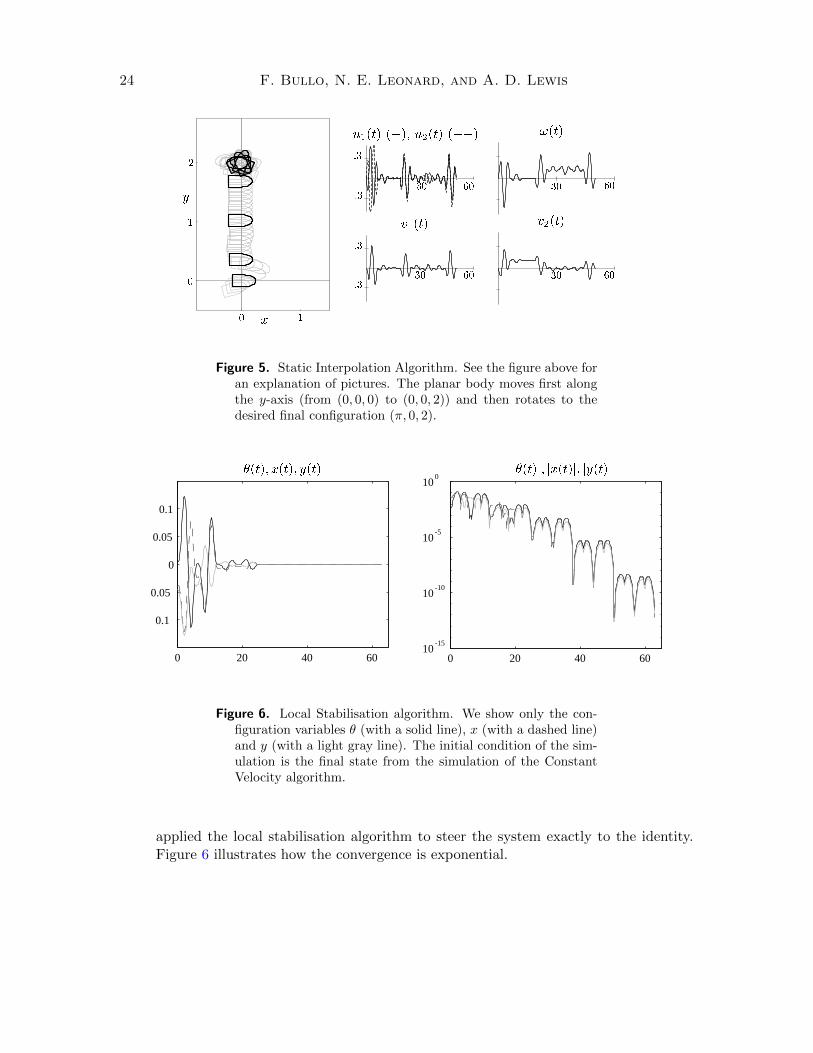
Static Interpolation, Table 3: For comparison, we next present the numerical resultsof the Static Interpolation Algorithm. The initial and final (desired) configurationsare the same as in the previous run. The set of ordered configuration points is(0, 0, 0), (0, 0, 2), (π, 0, 2). In Figure 5 one can notice the path in the x, y plane (con-sisting of a straight line and a rotation) and the various calls to the Change-Velocityand Maintain-Velocity primitives (for example, the time history of u1, u2(t) showspeaks whenever a Change-Velocity maneuver occurs).

Local Exponential Stabilisation, Table 2: Finally, we present the stabilisation algo-rithm. Starting from the final condition of the Constant Velocity Algorithm, we


Figure 5. Static Interpolation Algorithm. See the figure above foran explanation of pictures. The planar body moves first alongthe y-axis (from (0, 0, 0) to (0, 0, 2)) and then rotates to thedesired final configuration (π, 0, 2).

0 20 40 60

0.1

0.05

0

0.05

0.1

0 20 40 6010

-15

10-10

10-5

100

PSfrag replacements(t); x(t); y(t) j(t)j; jx(t)j; jy(t)j

Figure 6. Local Stabilisation algorithm. We show only the con-figuration variables θ (with a solid line), x (with a dashed line)and y (with a light gray line). The initial condition of the sim-ulation is the final state from the simulation of the ConstantVelocity algorithm.

applied the local stabilisation algorithm to steer the system exactly to the identity.Figure 6 illustrates how the convergence is exponential.


6. Conclusions

In this paper, we study motion planning and control of underactuated mechanical sys-tems with a focus on underactuated vehicles. We propose a geometric framework encom-passing analysis and synthesis tools and show its application to numerous examples. First,we characterise the controllability properties of these systems and investigate their be-haviour under small-amplitude forcing. Next, we design two motion primitives which weuse in higher-level motion control algorithms to steer the vehicle from point to point, tomove the vehicle between points in configuration space without stopping, and to provideexponential stabilisation of the vehicle to a desired configuration. Exponential stabilisa-tion is achieved using time-varying, continuous feedback control. The results in this papercomplement the controllability analysis of Lewis and Murray [1997a] and the averagingtechniques of Leonard and Krishnaprasad [1995]. Future research will focus on how toovercome the assumption of small-amplitude forcing and the absence of dissipation in ourmodels, see [Leonard 1995] for some results in this direction.

Acknowledgements. The first author thanks Prof. Richard M. Murray for his constantsupport. The research of the first author is, and of the third author was, supported inpart by the National Science Foundation under Grant CMS-9502224. The research of thesecond author is supported in part by the National Science Foundation under grant BES-9502477 and by the Office of Naval Research under grant N00014-96-1-0052. Dr Lewiswishes to acknowledge the Department of Control and Dynamical Systems which employedhim during the term in which this research was conducted.

References

Baillieul, J. [1993] Stable average motions of mechanical systems subject to periodic forcing,in Dynamics and Control of Mechanical Systems, The Falling Cat and Related Prob-lems, Fields Institute Workshop, (Waterloo, Canada, Mar. 1992), edited by M. J. Enos,1 Fields Institute Communications, pages 1–13, American Mathematical Society: Prov-idence, RI, isbn: 978-0-8218-9200-8.

Bonnard, B. [1984] Controllabilite de systemes mecaniques sur les groupes de Lie, SIAMJournal on Control and Optimization, 22(5), pages 711–722, issn: 0363-0129, doi: 10.1137/0322045.

Bullo, F. and Leonard, N. E. [1997] Motion control for underactuated mechanical systems onLie groups, in Proceedings of the 1997 European Control Conference, European ControlConference, (Brussels, June 1997), European Control Association.

Bullo, F. and Lewis, A. D. [1996] Configuration controllability of mechanical systems onLie groups, in Proceedings of 1996 International Symposium on Mathematical Theory ofNetworks and Systems, International Symposium on Mathematical Theory of Networksand Systems, (St Louis, MO, June 1996).

Crouch, P. E. [1981] Geometric structures in systems theory, Institution of Electrical Engi-neers. Proceedings. D. Control Theory and Applications, 128(5), pages 242–252, issn:1350-2379, doi: 10.1049/ip-d:19810051.

https://doi.org/10.1137/0322045

https://doi.org/10.1137/0322045

https://doi.org/10.1049/ip-d:19810051


Crouch, P. E. [1984] Spacecraft attitude control and stabilization: Application of geometriccontrol theory to rigid body models, Institute of Electrical and Electronics Engineers.Transactions on Automatic Control, 29(4), pages 321–331, issn: 0018-9286, doi: 10.1109/TAC.1984.1103519.

Fomenko, A. T. and Chakon, R. V. [1990] Recursion relations for homogeneous terms ofa convergent series of the logarithm of a multiplicative integral on Lie groups, Func-tional Analysis and its Applications, Translation of Rossiıskaya Akademiya Nauk. Funkt-sional ′nyı Analiz i ego Prilozheniya, 24(1), pages 48–58, issn: 0016-2663, doi: 10.1007/BF01077917.

Gurvits, L. [1992] Averaging approach to nonholonomic motion planning, in Proceedingsof the 1991 IEEE International Conference on Robotics and Automation, IEEE Inter-national Conference on Robotics and Automation, (Nice, France, May 1992), Instituteof Electrical and Electronics Engineers, pages 2541–2546, doi: 10.1109/ROBOT.1992.220059.

Kelly, S. D. and Murray, R. M. [1994] Geometric phases and locomotion, The Journalof Robotic Systems, 12(6), pages 417–431, issn: 1097-4563, doi: 10 . 1002 / rob .

4620120607.Khalil, H. K. [2001] Nonlinear Systems, 3rd edition, Prentice-Hall: Englewood Cliffs, NJ,

isbn: 978-0-13-067389-3.Lafferriere, G. and Sussmann, H. J. [1991] Motion planning for controllable systems without

drift, in Proceedings of the 1991 IEEE International Conference on Robotics and Au-tomation, IEEE International Conference on Robotics and Automation, (Sacramento,CA, Apr. 1991), Institute of Electrical and Electronics Engineers, pages 1148–1153, doi:10.1109/ROBOT.1991.131763.

Lamb, H. [1932] Hydrodynamics, Cambridge Mathematical Library, Cambridge UniversityPress: New York/Port Chester/Melbourne/Sydney, Reprint: [Lamb 1945].

— [1945] Hydrodynamics, Dover Publications, Inc.: New York, NY, isbn: 978-0-486-60256-1, Original: [Lamb 1932].

Leonard, N. E. [1995] Periodic forcing, dynamics and control of underactuated spacecraftand underwater vehicles, in Proceedings of the 34th IEEE Conference on Decision andControl, IEEE Conference on Decision and Control, (New Orleans, LA, Dec. 1995),Institute of Electrical and Electronics Engineers, pages 1131–1136, doi: 10.1109/CDC.1995.479226.

Leonard, N. E. and Krishnaprasad, P. S. [1995] Motion control of drift-free, left-invariantsystems on Lie groups, Institute of Electrical and Electronics Engineers. Transactions onAutomatic Control, 40(9), pages 1539–1554, issn: 0018-9286, doi: 10.1109/9.412625.

Lewis, A. D. [1997] Local configuration controllability for a class of mechanical systemswith a single input, in Proceedings of the 1997 European Control Conference, EuropeanControl Conference, (Brussels, June 1997), European Control Association.

— [1998] Affine connections and distributions with applications to nonholonomic mechan-ics, Reports on Mathematical Physics, 42(1/2), pages 135–164, issn: 0034-4877, doi:10.1016/S0034-4877(98)80008-6.

Lewis, A. D. and Murray, R. M. [1997a] Configuration controllability of simple mechanicalcontrol systems, SIAM Journal on Control and Optimization, 35(3), pages 766–790,issn: 0363-0129, doi: 10.1137/S0363012995287155.

https://doi.org/10.1109/TAC.1984.1103519

https://doi.org/10.1109/TAC.1984.1103519

https://doi.org/10.1007/BF01077917

https://doi.org/10.1007/BF01077917

https://doi.org/10.1109/ROBOT.1992.220059


https://doi.org/10.1002/rob.4620120607

https://doi.org/10.1002/rob.4620120607


https://doi.org/10.1109/CDC.1995.479226

https://doi.org/10.1109/CDC.1995.479226

https://doi.org/10.1109/9.412625

https://doi.org/10.1016/S0034-4877(98)80008-6

https://doi.org/10.1137/S0363012995287155


— [1997b] Decompositions of control systems on manifolds with an affine connection, Sys-tems & Control Letters, 31(4), pages 199–205, issn: 0167-6911, doi: 10.1016/S0167-6911(97)00040-6.

Manikonda, V. and Krishnaprasad, P. S. [1997] Controllability of Lie–Poisson reduced dy-namics, in Proceedings of the 1997 American Control Conference, American ControlConference, (Albuquerque, NM, June 1997), Institute of Electrical and Electronics En-gineers, pages 2203–2207, doi: 10.1109/ACC.1997.611084.

Marsden, J. E. and Ratiu, T. S. [1999] Introduction to Mechanics and Symmetry, A BasicExposition of Classical Mechanical Systems, 2nd edition, number 17 in Texts in AppliedMathematics, Springer-Verlag: New York/Heidelberg/Berlin, isbn: 978-0-387-98643-2.

M’Closkey, R. T. and Murray, R. M. [1997] Exponential stabilization of driftless nonlin-ear control systems using homogeneous feedback, Institute of Electrical and ElectronicsEngineers. Transactions on Automatic Control, 42(5), pages 614–628, issn: 0018-9286,doi: 10.1109/9.580865.

Morin, P. and Samson, C. [1997] Time-varying exponential stabilization of a rigid spacecraftwith two control torques, Institute of Electrical and Electronics Engineers. Transactionson Automatic Control, 42(4), pages 528–534, issn: 0018-9286, doi: 10.1109/9.566663.

Murray, R. M., Li, Z. X., and Sastry, S. S. [1994] A Mathematical Introduction to RoboticManipulation, CRC Press: Boca Raton, FL, isbn: 978-0-8493-7981-9.

Ostrowski, J. P. and Burdick, J. W. [1997] Controllability tests for mechanical systems withconstraints and symmetries, Journal of Applied Mathematics and Computer Science,7(2), pages 101–127, issn: 1641-876X.

Pettersen, K. Y. and Egeland, O. [1997] Robust attitude stabilization of an underactuatedAUV, in Proceedings of the 1997 European Control Conference, European Control Con-ference, (Brussels, June 1997), European Control Association.

Rathinam, M. and Murray, R. M. [1998] Configuration flatness of Lagrangian systems under-actuated by one control, SIAM Journal on Control and Optimization, 36(1), pages 164–179, issn: 0363-0129, doi: 10.1137/S0363012996300987.

Rui, C., Kolmanovsky, I. V., McNally, P. J., and McClamroch, N. H. [1996] Attitude controlof underactuated multibody spacecraft, in Proceedings of the 1996 IFAC World Congress,IFAC World Congress, (San Francisco, CA, July 1996), International Federation of Au-tomatic Control.

Sattinger, D. H. and Weaver, O. L. [1986] Lie Groups and Algebras, with Applicationsto Physics, Geometry, and Mechanics, number 61 in Applied Mathematical Sciences,Springer-Verlag: New York/Heidelberg/Berlin, isbn: 978-1-4757-1910-9.

Sørdalen, O. J. and Egeland, O. [1995] Exponential stabilization of nonholonomic chainedsystems, Institute of Electrical and Electronics Engineers. Transactions on AutomaticControl, 40(1), pages 35–49, issn: 0018-9286, doi: 10.1109/9.362901.

Sussmann, H. J. [1987] A general theorem on local controllability, SIAM Journal on Controland Optimization, 25(1), pages 158–194, issn: 0363-0129, doi: 10.1137/0325011.

Sussmann, H. J. and Liu, W. [1991] Limits of highly oscillatory controls and the approxi-mation of general paths by admissible trajectories, in Proceedings of the 30th IEEE Con-ference on Decision and Control, IEEE Conference on Decision and Control, (Brighton,UK, Dec. 1991), Institute of Electrical and Electronics Engineers, pages 437–442, doi:10.1109/CDC.1991.261338.

https://doi.org/10.1016/S0167-6911(97)00040-6

https://doi.org/10.1016/S0167-6911(97)00040-6

https://doi.org/10.1109/ACC.1997.611084

https://doi.org/10.1109/9.580865

https://doi.org/10.1109/9.566663

https://doi.org/10.1137/S0363012996300987

https://doi.org/10.1109/9.362901

https://doi.org/10.1137/0325011

https://doi.org/10.1109/CDC.1991.261338


A. Proofs

A.1. Proposition 4.1.

Proof: We start by proving the validity of the expansion in ξ(t, ε) by means of the standardperturbation method, as presented, for example, by Khalil [2001]. Consider the ordinarydifferential equation

x = f(x) + g(t, ε)

and let x(t, ε) denote the solution from initial condition x0(ε). At ε = 0, suppose thatf(x0(0)) = g(t, 0) = 0, so that x(t, 0) = x0(0) is a constant solution. We now expand x(t, ε)and g(t, ε) in a Taylor series about the value ε = 0 and write

x(t, ε) =∞∑i=0

εixi(t) and g(t, ε) =∞∑i=0

εigi(t).

As shown by Khalil [2001], the components in the expansion of x satisfy the followingdifferential equations

xn(t) =1

n!

∂n

∂εn

∣∣∣ε=0

f(x(t, ε)) + gn(t),

with initial condition xn(0) = 1n!

∂n

∂εn

∣∣∣ε=0

x0(ε).

The differential equation of interest in our case is equation (2.4):

ξ = −1

2〈ξ : ξ〉 + εb1(t) + ε2b2(t),

and the initial condition is ξ(0, ε) = εξ10 + ε2ξ2

0 . The constant solution we expand about isξ(t, 0) = ξ0(t) = 0.

Differentiating the function f(ξ(ε)) = −12〈ξ : ξ〉, we have

∂f

∂ε= −〈ξ :

∂ξ

∂ε〉

∂2f

∂ε2= −〈∂ξ

∂ε:∂ξ

∂ε〉 − 〈ξ :

∂2ξ

∂ε2〉

∂3f

∂ε3= −3〈∂ξ

∂ε:∂2ξ

∂ε2〉 − 〈ξ :

∂3ξ

∂ε3〉,

and noting that ∂n

∂εn

∣∣∣ε=0

ξ = n!ξn, we have

∂f

∂ε

∣∣∣ε=0

= −〈ξ0 : ξ1〉∂2f

∂ε2

∣∣∣ε=0

= −〈ξ1 : ξ1〉 − 2〈ξ0 : ξ2〉∂3f

∂ε3

∣∣∣ε=0

= −6〈ξ1 : ξ2〉 − 6〈ξ0 : ξ3〉.


Next, we write the differential equations as described above. Recalling that ξ0(t) = 0 wehave

ξ1 = b1

ξ2 = −1

2〈ξ1 : ξ1〉+ b2

ξ3 = −〈ξ1 : ξ2〉.Initial conditions are ξ1(0) = ξ1

0 , ξ2(0) = ξ20 , ξ3(0) = 0. Finally, we employ the notation

introduced in Section 5 to integrate the three ODEs,

ξ1(t) = ξ10 + b1(t)

ξ2(t) = ξ20 −

1

2〈ξ1

0 + b1(t) : ξ10 + b1(t)〉+ b2(t)

ξ3(t) = −〈ξ10 + b1(t) : ξ2

0 −1

2〈ξ1

0 + b1(t) : ξ10 + b1(t)〉+ b2(t)〉.

Expanding the terms on the right hand side, one recovers all of the terms in the expansionsof ξ(t, ε) in Proposition 4.1.

In the second part of the proof we prove the validity of the expansion of x(t, ε) by meansof the approximate solutions for kinematic systems obtained by Fomenko and Chakon [1990]and used by Leonard and Krishnaprasad [1995]. From these references we know that, ifξ(t, ε) = O(ε), then

x(t, ε) = ξ(t) +1

2

[ξ, ξ](t) +O(ε3).

Substituting ξ(t, ε) = εξ1(t) + ε2ξ2(t) +O(ε3), we have:

x(t, ε) = εξ1(t) + ε2ξ2(t) +1

2ε2[ξ1, ξ1

](t) +O(ε3).

And substituting the values for ξ1(t) and ξ2(t), and writing x(t, ε) = εx1(t)+ε2x2(t)+O(ε3),we have

x1(t) = ξ10 + b1(t)

x2(t) =

(ξ2

0t− 〈ξ10 : ξ1

0〉t2

4− 〈ξ1

0 : b1〉(t) +

(b2 − 1

2〈b1 : b1〉)

(t)

)+

1

2

[ξ1

0 + b1, ξ10 + b1

](t).

Expanding the terms on the right hand side, one recovers all of the terms in the expansionsof x(t, ε) in Proposition 4.1.

A.2. Lemma 4.2. Here, we prove the claim (4.7) in Lemma 4.2.

Proof: We start by studying the properties of the functions ψa(t). A direct computationshows that for all a, b, c

ψa(2π) = ψa(2π) = ψa(2π) = 0 (A.1)

ψa ψb(t) =δab2πt+ rab(t), where rab(2π) = rab(2π) = 0, (A.2)

ψa t (2π) = ψa ψb(2π) = ψa rbc(2π) = 0, (A.3)


where δab is the Kronecker delta function. The proof of these properties is straightforwardbut tedious.

Next, we prove the claim (4.7) in Lemma 4.2. Given the definition in equation (4.5)

and the property(A.2) of the functions ψa(t), we compute the quantity 〈b1 : b1〉(2π) as

〈b1 : b1〉(2π) =∑

1≤j<k≤m

∑1≤p<q≤m

√|zjkzpq|〈

(bj − sign(zjk)bk

):(bp − sign(zpq)bq

)〉ψa(j,k) ψa(p,q)(2π)

=∑

1≤j<k≤m|zjk|〈

(bj − sign(zjk)bk

):(bj − sign(zjk)bk

)〉

=∑

1≤j<k≤m|zjk|

(〈bj : bj〉 − 2 sign(zjk)〈bj : bk〉+ 〈bk : bk〉

)= −2

∑1≤j<k≤m

zjk〈bj : bk〉+∑

1≤j<k≤m|zjk|

(〈bj : bj〉+ 〈bk : bk〉

).

Summing up with b2(2π) = 2πb2, we have(b2 − 1

2〈b1 : b1〉)

(2π) =∑

1≤i≤mzibi +

∑1≤j<k≤m

zjk〈bj : bk〉,

which proves equation (4.7).

A.3. Primitives of Motion. The statements in the description of both primitives are directconsequences of the following result.

A.1 Proposition: Let the assumptions of Proposition 4.1 hold and let(b1(t), b2(t)

)=

Inverse(η). If ξ(0) = εξ10 + ε2ξ2

0, we have

ξ(2π) = εξ10 + ε2

(ξ2

0 − π〈ξ10 : ξ1

0〉+ η)

+ ε3π(π〈ξ1

0 : 〈ξ10 : ξ1

0〉〉 − 2〈ξ10 : ξ2

0〉 − 〈ξ10 : η〉

)+O(ε4)

(A.4)

x(2π) = ε2πξ10 + ε2π

(2ξ2

0 − π〈ξ10 : ξ1

0〉+ η)

+O(ε3). (A.5)

Proof: Note that property (A.1) implies directly that b1(2π) = b1(2π) = b1(2π) = 0, so thatthe terms in the Taylor expansion in Proposition 4.1 simplify to

ξ1(2π) = ξ10

ξ2(2π) = ξ20 − π〈ξ1

0 : ξ10〉+

(b2 − 1

2〈b1 : b1〉)

(2π),

ξ3(2π) = −2π〈ξ10 : ξ2

0〉+ π2〈ξ10 : 〈ξ1

0 : ξ10〉〉 − 〈ξ1

0 :

(b2 − 1

2〈b1 : b1〉)

(2π)〉

+ 〈〈ξ10 : ξ1

0〉 : b1〉 t2

(2π) + 〈b1 : 〈ξ10 : b1〉〉(2π)− 〈b1 :

(b2 − 1

2〈b1 : b1〉)〉(2π),

x1(2π) = 2πξ10 ,

x2(2π) = 2πξ20 − π2〈ξ1

0 : ξ10〉+

(b2 − 1

2〈b1 : b1〉)

(2π) + 12

[ξ1

0 + b1, ξ10t+ b1

](2π).


Hence, ξ1(2π) and x1(2π) are as computed above. We employ Lemma 4.2 and property (A.2)to simplify the remaining terms into

ξ2(2π) = ξ20 − π〈ξ1

0 : ξ10〉+ η,

ξ3(2π) = −2π〈ξ10 : ξ2

0〉+ π2〈ξ10 : 〈ξ1

0 : ξ10〉〉 − π〈ξ1

0 : η〉

+ 〈〈ξ10 : ξ1

0〉 : b1〉 t2

(2π) + 〈b1 : 〈ξ10 : b1〉〉(2π)− 〈b1 :

(b2 − 1

2〈b1 : b1〉)〉(2π),

x2(2π) = 2πξ20 − π2〈ξ1

0 : ξ10〉+ πη + 1

2

[ξ1

0 + b1, ξ10t+ b1

](2π).

Regarding the term ξ3(t), the claim is proven if

〈〈ξ10 : ξ1

0〉 : b1〉 t2

(2π) = 〈b1 : 〈ξ10 : b1〉〉(2π) = 〈b1 :

(b2 − 1

2〈b1 : b1〉)〉(2π) = 0.

However, since b1(t) is linear combination of the functions ψa(t), the latter relations cor-respond equality sign by equality sign to the properties in equation (A.3). Regarding theterm x2(t), it holds that[

ξ10 + b1, ξ1

0t+ b1](2π) = 2π2

[ξ1

0 , ξ10

]+

[ξ1

0 , b1(2π)

]+[b1, ξ1

0t](2π) +

[b1, b1

](2π) = 0,

as all terms in the middle expression vanish.

A.4. Lemma 5.2.

Proof: Given the descriptions of the primitives Change-Velocity and Maintain-Velocity,we compute the evolution of ξ(t) as follows. Starting from ξ(0) = O(σ2), we have:after first Change-Velocity(σ, ξnom) : ξ(2π) = σξnom +O(σ2),after first Maintain-Velocity(σ, ξnom) : ξ(4π) = σξnom +O(σ3),after kth step in the for loop : ξ(2(k + 1)π) = σξnom +O(σ3),after the final Change-Velocity(σ, 0) : ξ(2(N + 1)π) = O(σ2).

The final value of ξ is therefore as in the claim. Similarly, we can compute the change inconfiguration during each interval:after first Change-Velocity(σ, ξnom) : log

(g(0)−1g(2π)

)= πσξnom +O(σ3/2),

after first Maintain-Velocity(σ, ξnom) : log(g(2π)−1g(4π)

)= 2πσξnom +O(σ2),

after kth step in the for loop : log(g(2kπ)−1g(2(k + 1)π)

)= 2πσξnom +O(σ3),

after final Change-Velocity(σ, 0) : log(g(2Nπ)−1g(2(N + 1)π)

)= πσξnom +O(σ3/2).

We now need to sum the changes in configuration due to each interval by means of theapproximation in Lemma 5.1. Combining the contributions during the first two intervals,and recalling that [ξnom, ξnom] vanishes, we have

log(g−1

0 g(4π))

= 3πσξnom +O(σ3/2) =: 3πσξnom + σ3/2η1, (A.6)

where η1 = O(1) is an appropriate vector in g. Next, we claim that for all k = 1, . . . , N −1,it holds

log(g−1

0 g(2(k + 1)π))

= akξnom + σ3/2ηk,

where the scalar ak and the vector ηk are of order at most 1. We prove the claim byinduction. At k = 1, we recover equation (A.6), with a1 = 3πσ. Next, we assume that the


claim holds at k, and we prove it for k + 1. As dictated by Lemma 5.1, we compute thebracket between the current value akξnom +σ3/2ηk and the contribution 2πσξnom +O(σ3) =:2πσξnom + σ3ζk, where ζk = O(1) is an appropriate vector in g. We have:

[akξnom + σ3/2ηk , 2πσξnom + σ3ζk] = O(σ5/2),

so that

log(g−1

0 g(2(k + 2)π))

=(akξnom + σ3/2ηk

)+(2πσξnom + σ3ζk

)+O(σ5/2)

=(ak + 2πσ

)ξnom + σ3/2

(ηk + σ3/2ζk + σνk

),

where νk = O(1) is an appropriate vector in g. Hence, the claim holds at k + 1, withak+1 = ak + 2πσ and ηk+1 = ηk + σ3/2ζk + σνk. At the end of the for loop, as k = N − 1,we have

log(g−1

0 g(2Nπ))

= aN−1ξnom + σ3/2ηN−1,

where we can compute the coefficients as

aN−1 = a1 +N−1∑k=2

2πσ = (2N − 1)πσ and ηN−1 = η1 +N−1∑k=2

(σ3/2ζk + σνk

)= O(1).

The contribution of the last interval is σπξnom plus some higher-order terms, so that

log(g−1

0 g(2(N + 1)π))

= 2Nπσξnom +O(σ3/2).

Finally, we apply the approximation in Lemma 5.1 for a last time to obtain

log(g(2(N + 1)π)−1g1) = log((g−1

0 g(2(N + 1)π))−1(

g−10 g1

))= O(σ3/2),

where we recall that log(g−10 g1) = 2Nπσξnom and log(h−1) = − log(h).

A.5. Lemma 5.3.

Proof: We start by investigating the two Change-Velocity primitives described inside thewhile statement in Algorithm 2. Assuming that at time tk it holds∥∥( log(g(tk)), ξ(tk)

)∥∥ = σk 1,

we claim that ∥∥( log(g(tk+1)), ξ(tk+1))∥∥ = O(σ

3/2k ). (A.7)

This can be seen as follows. By assumption there exist two vectors xerr and ξerr of orderO(1) such that

log(g(tk)) = σkxerr

ξ(tk) = σkξerr.


With this notation, it holds −(

log(g(tk)) + πξ(tk))/(2πσk) = −

(xerr + πξerr

)/(2π). After

the primitive Change-Velocity(σk,−(xerr + πξerr

)/(2π)), we compute

log(g(tk + 2π)) = 12σk(xerr + πξerr) +O(σ

3/2k )

ξ(tk + 2π) = −σk(xerr + πξerr

)/(2π) +O(σ2

k),

and after the final Change-Velocity(σk, 0), we have

log(g(tk + 4π)) = O(σ3/2k ),

ξ(tk + 4π) = O(σ2k).

As tk+1 = tk + 4π, this proves equation (A.7). The latter equations are equivalent to∥∥( log(g(tk+1)), ξ(tk+1))∥∥ ≤Mkσ

3/2k , (A.8)

where the positive scalar Mk depends continuously on initial state and parameters of thesystem of ordinary differential equations (2.2) and (2.3). The parameters are σk and thecoefficients in the design of (b1(t), b2(t)), for tk < t < tk+1. By looking at the details of theinversion algorithm in Lemma 4.2, these parameters are seen to be continuous function of theinitial conditions

(log(g(tk), ξ(tk))

). Hence, we know that Mk(g(tk), ξ(tk)) is a continuous

function of its arguments and it is therefore bounded in a neighbourhood of the point(g(tk), ξ(tk)) = (Id, 0). In other words, there exist positive constants B1, B2 such that∥∥( log(g(tk)), ξ(tk)

)∥∥ < B1 =⇒ Mk(g(tk), ξ(tk)) < B2.

Finally, for some α < 1, we set σ = αmin(B1, 1/B

22

)and we prove by induction that

σk < σ and Mkσ1/2k ≤ α. At k = 0, we have by assumption

σ0 = ‖(log(g(0)), ξ(0))‖ ≤ σ < B1,

so that M0 < B2 andM0σ

1/20 < B2σ

1/2 < α < 1.

Therefore, the claim holds at k = 0. Next, we assume it at k, and prove it for k + 1. Werewrite equation (A.8) as

σk+1 =∥∥( log(g(tk+1), ξ(tk+1)

)∥∥ ≤ (Mkσ1/2k

)σk ≤ ασ < B1.

Hence, Mk+1 is also bounded by B2 and we have

σ1/2k+1Mk+1 ≤ σ1/2B2 < α.

This proves thatMkσ1/2k ≤ α for all k. In other words, we have that the sequence σk, k ≥ 0

satisfies σk+1 ≤ ασk with α < 1, or equivalently σk ≤ αkσ0. Therefore, for λ = − lnα > 0,∥∥( log(g(tk)), ξ(tk))∥∥ ≤ ∥∥( log(g(0)), ξ(0)

)∥∥ e−λk.Finally we prove the last statement in Lemma 5.3. From time tk to tk+1, the systemundergoes two Change-Velocity primitives and evolves starting from a state of order


O(σk) = O(e−λk) to a final state of higher order. During the two Change-Velocity

primitives, the input is of order√σk = e−λk/2 (with the notation in Section 5.1 and in

Proposition 4.1, it holds ε =√σ). Therefore, the expansions in Proposition 4.1 show that

the state is of order√σk = e−λk/2 from time tk to tk+1.

Controllability and motion algorithms for underactuated ...andrew/papers/pdf/1997b.pdf ·...

Documents

Transcript of Controllability and motion algorithms for underactuated ...andrew/papers/pdf/1997b.pdf ·...