CONTROL FOR SMALL OFFICE BUILDINGS
81
MICROPROCESSOR-BASED COOLING SYSTEM CONTROL FOR SMALL OFFICE BUILDINGS by CHI-SHING JOSEPH NG, B.S. A THESIS IN ELECTRICAL ENGINEERING Submitted to the Graduate Faculty of Texas Tech University in Partial Fulfillment of the Requirements for the Degree of MASTER OF SCIENCE IN ELECTRICAL ENGINEERING Approved Accepted May 1979
Transcript of CONTROL FOR SMALL OFFICE BUILDINGS

MICROPROCESSOR-BASED COOLING SYSTEM
CONTROL FOR SMALL OFFICE BUILDINGS
by
CHI-SHING JOSEPH NG, B.S.
A THESIS
IN
ELECTRICAL ENGINEERING
Submitted to the Graduate Faculty of Texas Tech University in Partial Fulfillment of the Requirements for
the Degree of
MASTER OF SCIENCE
IN
ELECTRICAL ENGINEERING
Approved
Accepted
May 1979

ACKNOWLEDGEMENTS
I am deeply indebted to Dr. Donald L. Gustafson for
his patient guidance and discussions through the course of
this investigation, also to Dr. Wayne T. Ford and Dr. K. S
Chao for their helpful suggestions and criticisms in the
preparation of this thesis.
11

TABLE OF CONTENTS
Page
ACKNOWLEDGEMENTS - - i i
LIST OF TABLES - -v
LIST OF FIGURES vi
I. INTRODUCTION - 1
II. COOLING LOAD CALCULATIONS AND ENERGY
ANALYSIS - - 5
2.1 Cooling Load Calculations - 5
2.2 Energy Consumptions 20
III. ENERGY MINIMIZATION CONTROL STRATEGIES 21
3 .1 Introduction - --21
3 . 2 Clock Control - 2 2
3.3 Operating Mode Selection 22
3.4 Start Time Optimization 23
3.5 Electric Demand Limiting 25
3.6 Increase Space Temperature and Relative Humidity - 28
3.7 Mixed Air Systems Optimization
Based on Enthalpy 29
IV. THE MICROPROCESSOR-BASED CONTROL SYSTEM 35
4.1 National Semiconductor PACE Microprocessor--35
4.2 Description of The Control System 37
4 . 3 Software System 40
4.4 Cost of The Control System 47
ill

V. COMPUTER SIMULATION RESULTS - 49
5.1 Introduction 49
5.2 An Example 49
5.3 The Office Room Characteristics -- 51
5.4 Energy Consumption for Different
Control Strategies - 57
VI. CONCLUSION- - - - 60
REFERENCES - --- -62
APPENDIX - - --64,
A.l Nomenclature of Chapter Two - 64
A.2 Multiplication Subroutine (MULT) 66
A.3 Division Subroutine (DIV) - 68
A.4 Truncation Subroutine (TRCS) --69
A.5 Search Subroutine (SEARCH) - --70
A.6 Interpolation Subroutine (INTER) 70
A.7 Approximation Subroutine (APPROX) 72
IV

LIST OF TABLES
TABLE PAGE
5.1 Average Seasonal Temperature Variations of Lubbock, Texas in 1961 52
5.2 Daily Energy Consumption for Typical Days in Spring, Summer, and Fall 52
5.3 Energy Consumption for Different Control Strategies during Occupied Period 58
5.4 Energy Consumption for Different Control Strategies during Unoccupied Period 58

LIST OF FIGURES
FIGURE PAGE
3.5 Forecasting Technique 27
3.7 Enthalpy Control Strategy 30A
4.1 Control System Hardware Organization 38
4.2 Block Diagram of Digital Controller Components -- 58
4.3 Flow Chart for Main Program 42
4.4 Flow Chart for Start-Time Optimization Subroutine 44
4.5 Flow Chart for Demand Limiting Subroutine 46
4.6 Flow Chart for Enthalpy Control Subroutine 48
5.1 Hourly Cooling Loads on May 13-14 (Spring) 53
5.2 Hourly Cooling Loads on June 27-28 (Summer) 54
5.3 Hourly Cooling Loads on Oct. 1-2 (Fall) 55
APPENDIX
A.2 Multiplication Subroutine (MULT) 67
A.3 Division Subroutine (DIV) 68
A.4 Truncation Subroutine (TRCS) 69
A.5 Search Subroutine (SEARCH) 71
A.6 Interpolation Subroutine (INTER) 73
VI

CHAPTER 1
INTRODUCTION
The utilization of air conditioning has made it possi
ble for man to live comfortably under severe climatic
conditions. In the United States, domestic air conditioning
began to develop rapidly after 1964. Since then almost all
commercial buildings have been equipped with air condition
ing systems.
The term air conditioning refers to the use of energy
to create and maintain an atmosphere having such conditions
as temperature, humidity, and air purity desirable for the
occupants of that space. Even though cooling methods have
changed greatly since the early days of air conditioning,
the fundamental problem, namely the conservation of energy,
remains.
Due to the accelerating cost of energy during the past
few years, the magnitude of the task of achieving energy
conservation is staggering. Numerous studies on the matter
of energy shortage lead one to believe that the U.S. demand
for energy will shortly outstrip her power generating
capacity and fossil fuel supply. According to a well quoted
report of the Stanford Research Institute (1), space heat
ing and cooling for residential and commercial buildings
amounts to approximately 20^ of the total energy consumption
1

in the country, which was 60 trillon Btu per year in 1968.
Reducing total energy used in all buildings by 301 without
impairing the indoor environment is a realistic and reason-
able goal.
Among all the energy used in an office building, about
701 is consumed in cooling and heating the space (2). Thus
air conditioning along with heating plays an important role
in our concern for energy conservation. In the present
study, only air conditioning is considered. This choice
does not imply that air conditioning is more important, but
was made because most of the control strategies used to
conserve energy during summer cooling seasons can also be
similarly applied to winter heating seasons.
Most of the buildings now in use were designed and
constructed when fuels and electric power were readily
available and inexpensive. At that time the need for energy
conservation was not important. The structures and their
mechanical and electrical systems were designed to minimize
initial cost, not energy usage. Buildings are generally
overheated in the winter, overcooled in the summer, over-
lighted, overventilated year-round, and not operated effici
ently. Each year they consume increasing amounts of energy
because systems and building components deteriorate as
maintainence and service becomes more costly and neglected.

3
The majority of the air conditioning systems today are
controlled either by semi-manual or analog methods which
consist primarily of pneumatic controllers. Although these
control systems are functionally reliable, they generally
do not minimize system energy requirements. Today the
application of digital control for air-handling equipment
appears to be a fruitful area for investigation.
It is recognized by the author that computer control
of building environmental system is not new. However,
the present computer control systems are complex and
expensive (3). They usually contain CRT displays, alpha
numeric keyboards, printers, etc.. These complex systems
are mostly employed in manufacturing plants, large office
buildings and airport terminals, they also control alarms,
smoke detectors, security, and building maintainence
instruction as well.
The low cost, miniature size, and the sophisticated
control capability of microprocessors establish them as
the most rapidly ascending stars in the computer galaxy.
One of the major advantages of microprocessor control, as
compared to analog control, is the programming flexibility
that a microprocessor exhibits in implementing control
strategies. It is the purpose of this study to evaluate
the potential of microprocessors in building automation

applications. The criteria for evaluation is to determine
if microprocessors can do more than conventional systems
to achieve energy conservation as well as low cost, so as
to establish that the microprocessor-based control system
is cost effective to install in small office buildings.
In this report the mathematical model and energy load
analysis of an air-conditioned space are given in Chapter
Two. Chapter Three discusses different energy saving
strategies and the merits of using microprocessors to
implement them. The microprocessor-based digital controller
is introduced in Chapter Four. In Chapter Five, a medium-
sized office room is used as an example to illustrate the
cooling load calculations and the results of energy analysis
for different control strategies. Finally, some concluding
remarks are given in Chapter Six.

CHAPTER 2
COOLING LOAD CALCULATIONS AND ENERGY ANALYSIS
2.1 COOLING LOAD CALCULATIONS
2.1.1 Introduction
A mathematical model which will account for the hourly
cooling loads of an air-conditioned space is going to be
developed in this chapter. The cooling load is the rate at
which heat must be removed from the space to maintain air
temperature at the assumed constant value. In order to
keep the air-conditioned space at the desired temperature
and humidity, the heat extraction rate from the space must
be approximately equal to the cooling load. Thus an
accurate mathematical model is needed both in predicting
energy consumption and in deciding the size of the air
conditioning system required for the space.
General cooling load calculations require consideration
of:
1) Building information and design conditions such as
building orientation, building materials, component
size, external shading, weather data, indoor
design temperature, etc..
2) Operating schedules of lighting, people, internal
equipment and applicance on weekdays, weekends and
holidays.
5

3) Instantaneous heat gain calculations including
internal and external heat sources.
4) Calculations of cooling load from instantaneous
heat gain.
The following sections will be devoted to partial
cooling load calculations from different heat sources,
i.e., heat gains from walls, roofs, glass area, infiltra
tion, equipment or electric appliance, lighting, and
people. Hourly total cooling load can then be calculated
from the total effects of these essential partial loads,
and total energy consumptions can be obtained.
2.1.2 Transient Heat Conduction Through Opaque W^alls
or Roofs
Conduction transfer functions are used widely and
considered as a convenient and effective tool for the
evaluation of transient heat transfer in building
construction components. The conventional steady state
heat transfer equation for calculation of heat gain:-^
Q = U (T^ - T^) C2a)
where
Q : heat gain or loss in Btu/hr
All the heat gains developed in this chapter are
on hourly basis.

a
To
U : overall heat transfer coefficient of roof or wall
T_ : inside air temperature
outside air temperature
is not sufficient for evaluating transient heat transfer.
This equation becomes invalid because the outdoor tempera
ture, T , usually varies due to solar radiation, cloud
cover and wind effect. The rapid change of the outdoor
temperature will not affect the room air unless the
structure is made up of the kind of materials which have
high heat conduction coefficients, such as galvanized steel.
Approximate calculation for a more accurate deter
mination of the instantaneous heat transfer can be made
by replacing the (T^ - T^) of equation (2.1) by a Total o a
Equivalent Temperature Difference (TETD) which is usually
precalculated for typical building construction components
and takes into account the thermal storage effect. Although
very useful, the TETD concept is only valid when the outside
temperature undergoes diurnal periodic changes. The TETD
concept is therefore especially useful in computing design
heat transfer rates for the building where very warm or
very cold conditions are assumed to occur for several
successive days.
A more accurate model which accounts for the effects
of randomly fluctuating outdoor conditions would use the

8
hourly history of temperatures in conjunction with heat
conduction transfer functions.
In order to calculate the convective energy transfer
between walls and room-air,the inside surface temperature,
Tg^, must be known. This can be determined by solving the
system of heat-conduction equations for a wall that consists
of J layers:
aT. 8^T. - ^ " j ^ Ij.i ^ X ^ 1. , j - 1,2...,J (2.2) 9t 3x^;
where
1 T. : temperature in the j layer of the wall
r\. : thermal diffusivity of the j^ layer of a surface 1" Vt
1- - In.2. • thickness of the j layer.
These equations must be solved subject to the following
boundary conditions: X = 1^ = 0; q = -k^ ^ = h^ (T^ - T^) ;
9X
X = 1^; j = 1,2---,J-1 ; Tj = T^^^ ;
Z T
where
q : heat flow going into the inside surface, Btu/hr
q, : heat flow leaving the outside surface, Btu/hr
k-, , kj : thermal conductivity of the inside and
outside surface

T^,Tj : temperature of the inside and outside surface
h-,hj : inside and outside surface heat transfer
coefficient,
and Qg j is the energy absorbed by an outside nonglass
surface and can be calculated as:
^ s u n " ^ •'•T
with a being the absorptivity of surface and I^ the total
solar radiation. In order to avoid the tedious and repetitive
solution of partial differential equations as part of the
overall cooling load calculations for a building, it is
advantageous to solve Eqs.(2.2) and (2.3) only once for a
set of construction materials in terms of so called
transfer functions (4). Wall heat fluxes and temperatures
can then be expressed in terms of previous values:
q = y X 7 T . . - T Y . T ^ • + C o q . 1 ° -=0 ^ s,in,i . Q 1 s,out,i R ^in,l
where
common ratio of the transfer function:
R " "T; T7~ Z,
T . •, T * • : inside and outside surface tempera-s,in,i* s,out,i ^

10
ture history of the surface i
^A-n 1 » Q«,,4. 1 • heat fluxes conducted in and out of 'in,i' ^out,l
the surface in the previous hour,
Btu/hr
Nj : number of nonzero terms in transfer function
relationship.
The X , Y , Z are the modified transfer functions which
have only Nj. nonzero terms. The value of N^ depends upon
the type of roof or wall construction. Generally heavy
construction requires a large value, although for most
conventional constructions, it seldom exceeds 20. Stephenson
and Mitalas have shown that the value of N , can be further
decreased by employing more than one past record of q (5).
The subscripts i in the equations denote the property at
time t - iAt. The method of finding these transfer func
tions has been discussed in detail in a National Bureau of
Standard Report (4), and will not be repeated here.
2.1.3 Heat Gain through Windows
The ability of glazing materials to transmit solar
radiation depends upon the wavelength of the radiation,
the thickness of the material, and the incident angle.
Virtually all types of glass are completely opaque to the
long wave radiation emitted by surfaces at temperatures

11
below about 250 F. This characteristic produces the green
house effect by which the solar radiation which enters
through a window is trapped. When the radiation is absorbed
by a surface within the room and then emitted as longwave
radiation, the heat cannot escape outward.
Heat transmitted through windows is affected by many
factors, of which the following are most significant :
1) Solar radiation intenisty, I^, and incident angle, e.
2) Outdoor-indoor temperature difference.
3) Velocity and direction of air flow across the
exterior and interior surfaces of the window.
When the window is irradiated by sunshine, the rate of
heat flow inward (6) by radiation and convection from an
unshaded single glazing is :
i " glass ^ V ^ + T - TJ (2.5) XT o a-o
where
U 1 : overall heat transfer coefficient of the glass
glass material
h^ : surface heat transfer coefficient. 0
Total instantaneous rate of heat gain through the glazing
material is the sum of transmitted and absorbed solar heat
gain, and conduction heat gain. Total heat gain per unit
area is expressed as :

12
Qglass = - IT * - ^T ^ K p * "glass ^ 0 " 3) (2-6)
where
T : transmissivity of glass.
When shading devices such as Venetian blinds, roller
shades, etc. are used, significant amount of heat gain
through window will be reduced due to the corresponding
change of T and U , ^ glass
2.1.4 Heat Gain from Infiltration
Infiltration may contribute a significant fraction to
the overall cooling load. Such infiltration heat gain
depends on the outside weather (temperature, humidity, and
primarily, wind speed and direction) as well as on the
quality of construction of the building under consideration
(crack sizes, etc.). Unfortunately, it is usually very
difficult, if not impossible, to estimate accurately crack
locations and sizes in a building. Furthermore, information
on frequency and timing of door and window openings or
closings are often insufficient.
Because of the above mentioned difficulties, infil
tration heat gain is generally estimated through the Air-
Change Method (7). This method assumes that the air inside
the air-conditioned space is exchanged for outside air a
number of times per hour, N^ ^^, e.g., between h and 2.
13
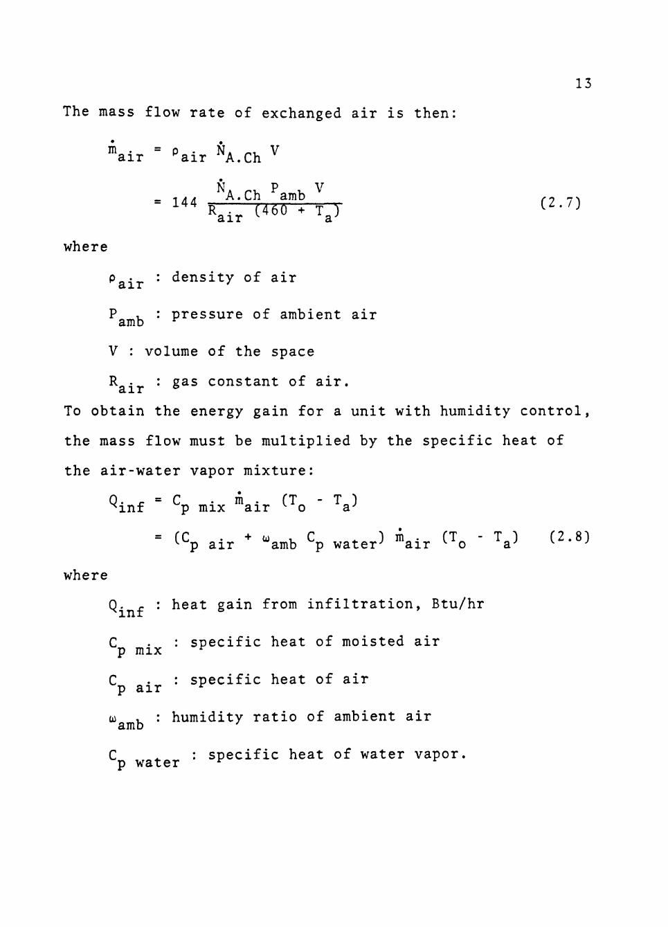
The mass flow rate of exchanged air is then:
ni • = p • N* i V air ^air A.Ch
= 144 A.Ch amb ^ j^ RTTrTTOnrin" C2.7) air a
where ^air * ^^sity of air
P r : pressure of ambient air
V : volume of the space
R«4« • gas constant of air. air ^
To obtain the energy gain for a unit with humidity control,
the mass flow must be multiplied by the specific heat of
the air-water vapor mixture: Q. n = C . m . (T - T„) ^ m f p mix air ^ o a-'
= (C . + w , C ^ ) in„. (T - T„) (2.8) ^ p air amb p water-' air ^ o a-* ^ •'
where
Q. r : heat gain from infiltration, Btu/hr
C . : specific heat of moisted air p mix ^
C . : specific heat of air p air ^
oj , : humidity ratio of ambient air
C ^ : specific heat of water vapor, p water ^ ^

14
2.1.5 Internal Heat Gain
Internal heat gain is the sensible and latent heat
released within the air-conditioned space by the occupants,
lights, appliances, machines, etc.. A portion of the
heat gain from internal sources is radiant heat which is
partially absorbed in the building structure, thereby
reducing the instantaneous heat gain.
Lights generate sensible heat by the conversion of
the electrical power input into light and heat. The heat
is dissipated by radiation to the surrounding surfaces, by
conduction into the adjacent materials and by convection to
the surrounding air. The radiant portion of the light
load is partially stored, and contributes to the space
cooling load after a time lag.
Incandescent lights converts approximately 10% of the
power input into light with the rest being generated as
heat within the bulb and dissipated by radiation, convec
tion and conduction. About 80% of the power input is
dissipated by radiation.
Fluorescent lights convert about 25% of the power
•'•Sensible heat is the energy involved in temperature
rise or fall; latent heat is the energy required to trans
form one pound of water into one pound of steam.

15
input into light, with about 25% being dissipated by
radiation to the surrounding surfaces. The other 50% is
dissipated by conduction and convection.
The heat generated from lights is expressed as :
Qi-ii- = 3413 QT . QI . , ^lite ^litx ^li.sch C2.9)
where
^litx * " ^ i" ^ energy output of lights per hour
in watts
^li.sch • igh^i^g schedule.
Most appliances contribute both sensible and latent
heat to a space. Electric appliances contribute latent
heat, only by virtue of the function they perform, that
is, drying, cooking, etc., whereas gas burning appliances
contribute additional moisture as a product of combustion.
A properly designed hood with a positive exhaust system
removes a considerable amount of the generated heat and
moisture.
Generally speaking, the entire wattage input to any
electrical heating appliance can be assumed to be converted
to sensible load. The rating printed on the nameplate
of the appliance is the value of watts input which should
be used. Again, as in the case of lights, the heat gain
from appliances is :

16
Q^„ = 3413 Q Q . (2.10) ^eq " eqx ^eq.sch ^ -'
where
Q^ : maximum energy output of equipment, watts
per hour
Q u ' equipment use schedule.
The human body in maintaining its temperature regula
tion must give off heat and must have moisture evaporated
from the skin. The percentages of the total heat given
off which are sensible heat and latent heat depend on
the degree of activity in which the person is engaged.
Generally speaking, the heat released by children is
about 50% of that for an adult under normal activities.
The sensible heat released by a normal person is :
Q = Q Q 1, ; ^occs ^os ^occ.sch *
and the latent heat is :
Q 1 = Q 1 Q V, (2.11) ^occl ^ol ^occ.sch ^
where
0 : sensible heat generated from an adult, Btu/hr ^os
Q , : occupancy schedule
Q , : latent heat generated from an adult, Btu/hr.
2.1.6 Cooling Loads
Cooling loads or room temperature can be obtained

17
by solving heat balance equations involving each of the
room surfaces. A room surface receives conduction heat
flow through the solid wall, roof or floor material from
behind, convection heat flow from the air and radiation
heat flow from other surfaces and internal heat sources
such as occupants, equipment and lighting fixtures.
The heat balance equation at the i surface at
any time is given by :
NR i ^ \ i , ''o ° J o ^ j . i ' ^s . in . j • J o ^ j , i ^ s . o u t . j
+ Cr. • Q • 1 R , i ^ i n , l
NS
- " i ^ \ ' Ts , in , i ^ ' J , ^ i ,k ^^s, in,k - ^ s , i n , i ^
•*• T ( 2 . 1 2 )
where
G. ^ = ( 4 ) ( 0 . 1 7 1 4 ) ( 1 0 " ^ ) e . F.^^^ (T^ + 460)^
T = ^T,i ' ^ ^ ^ ^^- ^^ % * ' - o V c
i-1 ^
^ CI - %) Qute >
with S. and e. being the area and the emissivity of the
i" ^ surface, F. , being the radiation view factor between 1 ,x
the i^^ surface and the k^^ surface, and NS being the
number of surfaces. And R , R , R, are the fractions of w ^J ^

18
heat gain from equipment, lights, and occupants, which
can be assumed to be convective. The heat balance equation
for the room air is :
NS S. TT . . - T 1 + 0. . + m _ - ,-
sa p mix ^ sa a
I S. (T . . - T ) + Q. r + in C . (T - T ) j ^ 1 ^ s,in,i a-' ^mf -^ ' ^^ ^^^ ^
+ Q^ioo. + Q R + Q R + Qi-^ R, = 0 (2.13) ^glass eq e ^occ o ^lite 1 ^ ^
where
m : mass flow rate of supply air s a
T : temperature of supply air. s a
Assigning matrix elements for i = 1,2,««',NS and for
k = 1,2,.-.,NS :
NS A. .. = H. I. • • — H • **• ) G . I 1,1 1 ^ti ^>^
\,k ^ "^i,k " \,i " ' k,i
^i,NS+l " ""i
%.i . ^R,i i ' • Jo ^j,i ' s,in,j "" J Q ^j,i ' s,out,j
- ^R,i ^in,l " T
\s+l,k " k \ NS
^NS+1,NS+1 = " C" air ^ a^ S mix ^ J^ "k k
^NS+1 " " eq e " occ o " lite 1 " air S mix 'o
- m C - T - Q -, sa p mix sa ^glass
Then Eqs.(2.12) and (2.13) can be written in matrix form

19
as :
1,1
2,1
1,2 •
7,2 •
. A 1,NS+1
. A 2,NS+1
'NS,1
'NS + 1,1
^NS,2* • • ^NS,NS+l
^NS+1,2* • ^NS+1,NS+1
s,in,l
s,in,2
s,in,NS
B.
B,
\^S+1
The above NS+1 equations should be solved simultaneously
for T . • . with i = 1,2,---,NS, and for T .
When the value of T has been specified, as in the
case of a constant temperature condition, the following
NS equations should be solved instead of the NS+1
equations given above :
1,1
A 2,1
^1,2 • • • "^1,NS
"^2,2 ' • • '^2,NS
'NS,1 ^NS,2- • • '^NS,NS
s,in,1
s,in,2
T s,in,NS B NS
where
^i " ^i • ^i,NS+l " a

20
The sensible load is then calculated as :
NS QcT = y S. (T . . - T ) + Q. ^ + m C • (T
i=l ^ s,in,i a ^mf sa p mix ' sa
T ) + Q i + Q R + Q R + Q , . ^ R i a^ ^ g l a s s ^eq e ^occ o ^ l i t e 1
( 2 . 1 4 )
This is the heat picked up by the room air which has to be
removed by the air-conditioning system. The latent load
is the same as the latent heat gain if moisture and
absorption by room walls, or drying of the wall panels
can be neglected.
2.2 ENERGY CONSUMPTIONS
Energy is required to remove the hourly cooling load
so that the air-conditioned space is maintained at the
desirable conditions. In order to obtain the hourly
energy consumption, a partial load performance curve of
the cooling system in use is referred to and the energy
consumption for each corresponding cooling load is obtained
from the curve.
A mathematical model for cooling load calculations
has been developed in this chapter. In the next chapter,
energy minimization control strategies will be developed,
and some of these control strategies can be evaluated by
the mathematical model on an energy conservation basis.

CHAPTER 3
ENERGY MINIMIZATION CONTROL STRATEGIES
3.1 INTRODUCTION
Energy analysis for an air-conditioned space has
been done in the last chapter. In this chapter, some
energy minimization control strategies will be developed
for the model. The most promising ones will be implemented
in software algorithms in the microprocessor-based control
system in the next chapter.
Some of the automation and energy conservation
strategies involve the whole space under control, while
others are limited to a specific group of equipment. For
each of the many potential energy minimization strategy,
all three levels--semi-manual, analog hardware and micro
processor control will be reviewed. When it appears that
the microprocessor control is superior for a particular
task, the reasons for that will be stated.
A microprocessor combined with memory and I/O devices
is itself a complete microcomputer, which is important
because its small size and low cost make the power of
computers available for a vast new range of applications.
Of course, any computer system can do everything that a
microprocessor-based system is able to control and even
more. But due to the high cost of full-sized computer
systems, owners of small commercial offices can hardly
21

9 -
afford one. Thus the use of computers in building control
will not be considered here.
3.2 CLOCK CONTROL
All three levels of automation can handle the task
of turning the system on and off as a function of time, but
the microprocessor implementation is more flexible, easier
to modify, less subject to human error and more suited
to unattended operation.
3.3 OPERATING MODE SELECTION
In order to maximize energy conservation, the control
system must be able to determine the mode of operation
which the building is in. The control system has different
functions in each of the operating modes :
SS - summer startup
WS - winter startup
0 - occupied
U - unoccupied
N - normal
E - emergency
Microprocessor implementation of this task is clearly
superior to the other two levels of automation. If micro
processor control is not used, it is better off to make
the operating mode selection manually than to rely on the
conventional analog hardware.

1 -7 i . w)
3.4 START-TIME OPTIMIZATION
The purpose of start-time optimization is to produce
a comfort condition at the time of occupancy for buildings
that shut down the mechanical equipment. For 24-hour
operational buildings (such as hospitals), start-time
optimization will be of no value.
Cooling machines and fan systems are started so that
comfort conditions will be reached at occupancy time with
out any waste of prime energy. Start-time is dependent
upon space conditions and outdoor conditions. The building
equipment and fan systems should be logically grouped so
that the start-up of groups of equipment are properly
sequenced. In addition to the proper sequencing, other
parameters must be considered in start-time optimization:
the time interval between equipment in the same start-up
group, the outside air damper position during the start
up time, and the day of the week. The time interval may
be predetermined when based on the nature of equipment
used. For purposes of energy conservation, the outside
air dampers should be kept closed during the start-up
period unless it is advantageous to use outside air.
The chiller plant start-up time should include the
hydraulic lag time and the equipment time delays. The
fan system start-up time must include a nominal time
24
interval for the fresh air intake and circulation.
The basic start-up units are fan systems. One or
more fan systems can be started as an individual start
up group. The fan system with the longest start-up time
will determine the chiller plant start-up time. The
space temperature for each fan system is the temperature
at the representative point in the spaces served by the
fan system. In essence, the program stored in the micro
processor system generally checks the space temperature
of a given start-up group and the outside air conditions
to determine the start-up time. The start-up program is
activated one or two hours prior to the occupancy time
at certain time intervals.
The program will check outdoor conditions, scan
space temperature, and compare them with stored tables
for start-up time. The stored tables are either estimated,
based on historical data; or calculated, depending upon
the building heat transfer characteristics through an
energy analysis program. When actual start-up data is
accumulated, the stored data may be modified for better
start time accuracy and maximum operating efficiency.
This type of operation is ideally suited for micro
processor control while it cannot be fully implemented
with analog hardware.

25
3.5 ELECTRIC DEMAND LIMITING
The electricity bill for commercial buildings is
composed of total electric energy consumption and demand
charge. The demand charge is based on the highest average
electrical load occuring in a demand period. Depending on
the power company rate schedule, a 15 minute demand period
is generally used, but occasionally a 30 or 60 minute
period is used. Rate schedules vary substantially between
power companies. In some rare cases where there is no
demand charge, the demand limiting is of course of no
value to the owner. Therefore, the object of demand
limiting is to avoid establishing a new higher peak and
confine demand within a preset limit.
Typically, the power company installs, in addition to
the energy meter, a demand meter which has an internal
clock and counter. The clock resets the counter at demand
intervals. During the demand period, the counter is
advanced with each revolution of the watt-hour disc. At
the end of the period, the quantity accumulated by the
counter is recorded immediately preceding counter reset.
Most power companies furnish auxiliary contacts which are
synchronized with the counter advances and counter reset
of the demand meter. Closures of the contacts can be
detected by the automation system, and proper action can
be taken to limit the demand during this period.

26
For billing advantages, it is desirable to limit the
peak demand below an optimal level. This can be accomplished
by shedding selected nonessential loads in a building during
the peak demand period. These nonessential loads can be
determined by the building manager and are highly dependent
upon the nature of the building and the available sheddable
devices. In general, corrider lights; garage lights;
certain fans; pumps; heat transferring equipment with long
time lags; and certain electric heat terminal units can
be used for shedding electrical loads. If the lighting
level permits, reducing lighting level results in savings
in demand, power consumption, and decreased cooling load.
A common forecasting method (Fig. 3.5) can be used to
compute the current demand rate and project the demand
value at the end of the demand interval. In other words,
the average rate of electrical load occurence up to the
time of computation is used to project the ultimate value
at the end of the demand period. Should the predicted
value exceed the preset limit, load shedding will take
place to prevent excessive electric demand during this
period.
Moreover, the load shedding devices may be grouped
so that the priority of shedding can be handled in a
rotating manner. In other words, the same device will
not be turned off every time. Groups of equipment will

27
3 4 5 6 7 8 9 10 11 12 13 14 15
Time, minute
Fig. 3.5 Forecasting Technique

28
share in a certain manner so that all the load shedding
devices are properly distributed in the load shedding
schedule.
Peak shedding can be implemented by all three levels
of automation. In comparision with a semi-manual approach,
microprocessor implementation eliminates human error and
the need for continuous observation by the operator. In
comparision with the use of demand limiting hardware
packages, microprocessor control is superior because it
is easily reprogrammable and flexible. This makes it
easier to adopt to changing operating conditions.
3.6 INCREASE SPACE TEMPERATURE AND RELATIVE HUMIDITY
3.6.1 Occupied Period
The air conditioning systems in many buildings were
designed to maintain 72 to 75 F D.B. and 50% R.H. during
peak loads in the cooling season. They are operated to
maintain these levels at peak conditions, and to achieve
even lower levels during the part load conditions which
occur most of time.
A substantial amount of energy will be saved if the
indoor temperature and humidity levels are allowed to
increase from 74 F D.B. and 50% R.H. to 78 F D.B. and
60% R.H., as recommended by the Federal Government.

29
3.6.2 Unoccupied Period
Energy will be saved if the space temperature is
allowed to increase up to 85 F during unoccupied period.
However, due to the heat storage effect of building
construction materials, there will still be existing
cooling loads in the space for the first few hours of an
unoccupied period, and the cooling system is still required.
But in geographic areas which usually have relatively
chilly nights like Lubbock, temperature in the space at
night can be allowed to 'float'. It is advantageous to
have an air damper or a window open so that natural
ventilation and infiltration alone will eventually cool
off the space.
3.7 MIXED AIR SYSTEMS OPTIMIZATION BASED ON ENTHALPY
In recent years an economizer cycle has been frequently
used in controlling the mixed air system. This system
controls the use of minimum outside air or the mixture of
outside air and return air based on dry-bulb temperature
only. Because the economizer cycle is only based on the
dry-bulb temperature and not the total heat content of
air, there are times when minimum outside air is more
economical but mixed air is called for. Conversely, there
are times when a mixture of outside air and return air is
more economical but a minimum amount of outside air is used.

30
The enthalpy of the air is based on both the dry-
bulb temperature and the moisture content of the air. The
moisture content can be determined by measuring the
relative humidity or wet-bulb temperature of the air.
The enthalpy optimization by the microprocessor-
based system is to determine the outside air and the return
air ratio based on enthalpy calculations. To minimize
energy consumption, the outside air and return air enthalpy
are calculated so that the precise mixing ratio will
satisfy the need of the space at a minimum cost of prime
energy.
The basic logic of enthalpy optimization can be
implemented in many ways. When the outside air dry-bulb
temperature is below the cooling coil discharge temperature,
there is no need for cooling. In this case, a mixture of
outside air and return air will satisfy the cooling needs
(Fig. 3.7, Region I). The cooling coil is generally
controlled within an operating range. But, at any instant,
the control point is fixed. The discharge temperature
control of the cooling coil must be stable before the
enthalpy optimization can be meaningful. Fig. 3.7 shows
a typical enthalpy optimization logic diagram. This method
assumes that the ideal return air dew point is near the
Heat content in Btu/lb.

3 0A'
0)
cd
o
o u
Cd
• H

31
cooling coil discharge temperature. In other words, no
moisture gain or loss is assumed in the building. It
further assumes the non-existence of an extremely dry
climate. On this basis, typical enthalpy optimization
logic is developed.
It is simple to understand the essence of Fig. 3.7
type enthalpy optimization logic from the following
examples :
Example 1 : Assume outside air conditions are :
Outside air dry-bulb temperature : DB = 95 F * oa
Outside air dew point temperature : DP^ - 60 F
The enthalpy that can be found from a psychrometric chart
is 35.4 Btu/lb. If the return air conditions are :
Return air dry-bulb temperature : DB = 77 F
Return air dew point temperature : DP = 55 F
The enthalpy is approximately 28,7 Btu/lb. It is apparent
that the outside air dew point and dry-bulb are both
higher than that of the return air. Therefore, if the
cooling coil must condition the mixed air to a desirable
level, say 55 F dry-bulb at near saturation, the outside
air will require more energy to remove the latent and
sensible heat than that of the return air. The apparent
solution is to use minimum outside air. Therefore, when
enthalpy of outside air is higher than that of return

32
air, minimum outside air should be used.
Example 2 : Assume the outside air conditions are :
DB^^ * 75 F oa
DP^^ = 64 F oa
The enthalpy of the outside air is approximately 32.2
Btu/lb. Assume the same return air conditions as in
Example 1 :
DB^^ - 77 F ra
DP^, = 55 F ra
It is seen that the return air enthalpy is only 28.6
Btu/lb. Although the dry-bulb of outside air is lower
than the return air dry-bulb, the latent load in the outside
air is much greater than that of the return air. Therefore,
it is advantageous to use minimum outside air.
Example 3 : Assume the same return air conditions as in
Example 1. Let :
DB = 67 F oa
DP^, = 57 F oa
In this case, there is more latent load in the outside
air than in the return air. However, the sensible load
of the outside air is much less than that of return air.
The total latent and sensible heat removal of the outside
air (27.1 Btu/lb) is less than that of return air (28,6
Btu/lb). Therefore, it is advantageous to use 100% outside
33
air again.
Example 4 : Assume the outside air conditions are :
DB^^ = 40 F oa
I P o = 35 F oa
In this case, a mixing of outdoor air and return air will
provide the proper mixed air requirement. No cooling is
necessary. Therefore, it is advantageous to turn off the
cooling coil and use mixed air control only.
Based on the above examples, it can be concluded
that :
1) When the outside air enthalpy is greater than
that of the return air or when the outside air
dry-bulb is greater than that of the return air
(Region III), the outside air damper must be set
to minimum.
2) When the outside air enthalpy is below the return
air enthalpy and the outside air dry-bulb is
below the return air dry-bulb but above the cool
ing coil discharge control point (Region II),
100% outside air must be used.
3) When the outside air enthalpy is below the return
air enthalpy and the outside air dry-bulb is
below the return air dry-bulb and below the cool
ing coil controller setting (Region I), the mix
ing dampers must be used.

34
This method of optimization can be implemented by all
three levels of automation, but microprocessor control is
superior. This is because manual damper optimization is
expensive due to the need for continuous operator involve
ment. Analog implementation is even more expensive
because an extensive hardware package is needed to evalu
ate the outside air on an enthalpy basis. Most presently
available hardware packages provide only partial optimiza
tion (8) . They frequently evaluate the outside air on the
basis of temperature only and not on enthalpy.

CHAPTER 4
THE MICROPROCESSOR-BASED CONTROL SYSTEM
Some energy minimization control strategies for an
air-conditioned space were developed in the last chapter.
In this chapter, the implementation of the control system
will be discussed, and the software system for the energy
minimization algorithms will be developed for the National
Semiconductor PACE Microprocessor. The PACE is one of the
few 16-bit microprocessors available, and the only one made
with a low-cost PMOS process. It can operate with just a
single-phase clock, and still deliver much of the perform
ance formerly requiring a minicomputer. In the implementa
tion here, 16-bit microprocessor is more convenient in
data manipulation, and the unique feature of PACE in memory
and I/O device addressing makes data flow easily on the
bus. Of course, before developing the software, it is
necessary to consider the features of the microprocessor
in use in more detail.
4.1 NATIONAL SEMICONDUCTOR PACE MICROPROCESSOR
PACE (Processing and Control Element) is the first
16-bit, single chip microprocessor developed by National
Semiconductor from the implementation of its multi-chip
35

36
product IMP-16. It is packaged in a standard, hermetically
sealed, 40-pin ceramic dual-in-line package.
PACE has seven data registers, four of which, AGO to
AC3, are directly available to the programmer for data
storage and address formation. AGO and ACl are the work
ing registers, and AC2 and AC3 are page pointers or auxi
liary data registers. The other three registers serve as
a program counter (PC). A 16-bit push-pull stack is also
provided for additional data storage for up to 10 words.
The programmer can specify the PACE ALU to operate
on either 8- or 16-bit data through the use of a byte
flag. All status and control bits are provided in a
single status flag register, which includes the status
bits for carry, overflow, link, etc. The execution time
for an instruction is in the range of 8 to 20 microseconds
when a 500-nanosecond clock is used. All data transfers
between PACE and external memories or peripheral devices
take place over the 16 data lines (D00-D15). All memory
addresses of PACE are shared by memory and I/O devices.
In connection with the memory, measuring devices,
A/D and D/A converters, buffer devices and some necessary
interface circuits, the PACE can be an independent
controller. It receives input from the measuring devices,
process it through the control program stored in the

37
memory, and output the control signal to the actuator of
the controlled system.
4.2 DESCRIPTION OF THE CONTROL SYSTEM
The control system hardware consists of four basic
components (Fig. 4.1) : (1) the digital controller and
associated interface, (2) the control console, (3) the valve
and damper station, and (4) the sensing devices.
The digital controller (Fig. 4.2) consists of the PACE
Microprocessor; approximately 2K of ROM memory to store the
energy minimization control program; IK of RAM memory,
which will have battery backup so that system status and
data are lost during a power failure, is used to store
current data and system status; a A/D converter; a multi
plexer which will accomodate 16 process signals; signal
conditioners; a D/A converter; and interface logic. This
unit will be the heart of the system. It will perform all
data acquisition, control and optimization calculations,
valve and damper activation, as well as communications
with the control console and/or a host microprocessor
which manages all the digital controllers of the building.
The control console will provide for communications
with the control system for both process monitoring and
table update.

Sensing
Devices ->
Control
Console
TTNT
^
Digital
Controller ^
38
^
Valve and
Damper Station
Fig, 4.1, Control System Hardware Organization.
2K ROM
Memory
A/D
Converter 77
<,<
Parallel
Interface
Analog Multiplexer
7K^
Analog input signals
from signal conditioners
IK RAM
Memory
J_ PACE
Microprocessor T7
Serial
Interface 7f^
Control
Console
<: t' Parallel
Interface
D/A
Converter
Output con
trol signals
Fig. 4.2. Block Diagram of Digital Controller Components

39
The valve and damper station will contain the interface
between the valves or dampers and the digital controller.
It should be such designed that manual control over the
valves and dampers can be employed in emergency situations
or microprocessor failure.
The sensing devices are analog sensors for dry-bulb
temperature, wet-bulb temperature, and humidity. Two pairs
of dry-bulb and wet-bulb temperature sensors are used.
One pair is located at the outdoor side of the controlled
space to measure outside conditions, another one is at
the inlet of the return air damper to measure return air
conditions. Also, a set of dry-bulb temperature and
humidity sensors is mounted on one of the walls not adjacent
to any heat sources to measure room conditions. And two
flip-flops are provided to detect the closures of the
demand meter auxiliary contects.
In addition to the four basic components, the control
system will also have a digital calender clock that records
both the day and the time of the day so that different
control conditions can be applied for weekdays and weekends.
In order to maintain correct time in case of an outage, the
clock should have a battery-charging circuit. Timers are
available for the system to trigger inputs to the micro
processor at certain preset time intervals.

40
4.3 SOFTWARE SYSTEM
In developing the operational subroutines for data
manipulations, the basic set-up form of a number is necessary
to be considered. In the PACE Microprocessor, the binary
bit is the basic unit, and eight bits form a byte. Each
accumulator of the microprocessor and each memory location
is able to store a 2-byte word. Here, two bytes will be
used to represent any number so that double-precision can
be obtained with single-word instructions.
Although floating point representation is convenient
in such a way that it offers a means to automatically keep
track of the decimal point. But from the microprocessors
point of view, it is more complicated to build a floating
point operating system than to build an integer operating
system. In order to build an integer operating system, the
inputs and the data stored in the memory should be appropri
ately scaled up so that the microprocessor only operates
on integers.
Binary representation of numbers will be used as it
has both speed and memory storage efficiency advantages
over BCD form of numbers. However, space temperature and
humidity inputs may be converted to BCD form for display
purpose.

41
4.3.1 Main Program
The main program implements all the energy minimization
control strategies discussed before. It contains time of
day control, operating mode determination, start-time
optimization, demand limiting, and enthalpy control. The
program checks for the day of the week and the time of the
day so that different temperature and humidity profiles can
be used accordingly. The start-time optimization subroutine
is called 1 hour before the occupied period to obtain the
optimal start-time for each start-up group. For any time
during the occupied period, should the space temperature
rise higher than 85 F, the system will be in emergency mode
and proper actions will be taken. Enthalpy of both outside
air and return air are calculated and are compared frequent
ly so as to determine the proper amount of air from outside
to be used for the interval between two consecutive calcu
lations. During a demand interval, the demand limiting
subroutine will be used to predict and limit the demand.
The flow chart is shown in Fig. 4.3.
4.3.2 Start-Time Optimization Subroutine
For each start-up group of equipment, a two-dimensional
table, which contains optimal start-times for different
combinations of inside and outside temperatures, is stored
in the memory. In order to minimize the size of the table.

42
MAIN
YES.
NO
YES
occupied period profile
Operating mode is N
J ^
Call ECS
Weekend profile Operating
mode is WS
Unoccupied period profile
Operating mode is SS
Call STS
Operating mode is E
YES Call DLS
Fig. 4.3. Flow Chart for Main Program.

43
all the inside and outside temperature coordinates of the
table are in integer form. For an input temperature that
is to the tenth of an integer, the fractional part will be
truncated and the input be approximated to the whole
integer yalue so that the table can be used. For example,
if the inputs of the inside and outside temperatures are
66.3 and 75.8 respectively, then these values will be
approximated to 66 and 75, and the optimum start-time is
the entry of the table corresponds to an inside temperature
of 66 F and an outside temperature of 75 F.
The start-up groups will be of such sequence that the
one requires the longest start-up time is serviced first.
And it is assumed that inside and outside temperature
inputs are available when the subroutine is called. The
flow chart is shown in Pig, 4.4.
4,3.3 Demand Limiting Subroutine
Whenever the synchronous flip-flop is set, the air-
conditioned space starts to be under a demand interval.
This subroutine is used to predict the power demand at the
end of the interval so that shedding will take place if
the predicted yalue exceeds the preset limit. It starts
calculating the predicted demand two minutes before the
end of the interval, for a period of 1,5 minutes, and the

STS
44
1L5-
GN = 1
><-
NO
JAL
Call APPROX
<r
Call SEARCH to get t
^
t = t - t^ c o
GN : start-up group
number
TN : total number
of groups
t : time on calen-c
der clock
t : time starts 0
occupied period t : start-time s
from the table
YES
GN = GN +1
YES
RET
Fig. 4.4 Flow Chart for Start-Time Optimization Subrou
tine.

45
predicted value will be renewed every time a higher value
occurs.
The rate of the electric demand occurence is calculated
every second. The demand prediction is done according to
the average rate of the demand curve, and the value of the
meter counter at time of computation :
PV = R (TT - N) + PR
where
PV : the predicted value
R : average rate
TT : length of the demand interval in seconds
N : number of seconds elapsed
PR : present value of the counter.
The flow chart is shown in Fig. 4.5.
4.3.4 Enthalpy Control Subroutine
A two-dimensional enthalpy table is stored in the
memory for different combinations of dry-bulb and wet-bulb
temperatures that are likely to occur. In order to minimize
the size of the table, all dry-bulb and wet-bulb temperature
coordinates of the table are in integer form, and wet-bulb
temperature coordinates are given in increment of five.
Interpolation scheme is used to find corresponding enthalpy
for those wet-bulb temperature values that lie in between

\ f
N = N + 1
^ /
R = RATE + R
46
^ Reset F/F
^
Set control F/F
Calculate PV
'><r
RET
Fig. 4.5 Flow Chart for Demanding Limiting Subroutine

47
the coordinates. For an inputting dry-bulb temperature
with fractional part, it will be approximated to the whole
integer value as described before.
For outside air condition being in Region I as shown
in Fig. 3.7, mixture of return and outside air will be
supplied to the space, and the percentage of outside air
used will be determined by :
X E^ + (1 - X) E^ = E^
where
X : percentage of outside air used
E^ : enthalpy of outside air
E^ : enthalpy of return air
Eg : enthalpy of supply air which is used to maintain
the space condition at 75 F and 60% R.H.
Assume all outside air and return air temperature
conditions are available when the subroutine is called.
The flow chart is shown in Fig. 4.6,
4.4 COST OF THE CONTROL SYSTEM
Total implementation cost of the control system depends
on specific components used. Speaking of mass production,
the total cost will be amounted to approximately five-
hundred dollars for all the hardware components and soft
ware programming.

ECS 48
YES
Call APPROX to get inte-ggr DBQ, DBr
Call INTER to get EQ
Call INTER to get Ey
DB
DB.
outside air temperature
return air temperature
YES. Calculate % of outside air
YES 100% outside
air
Minimum
outside air RET
Fig. 4.6 Flow Chart for Enthalpy Control Subroutine

CHAPTER 5
COMPUTER SIMULATION RESULTS
5.1 INTRODUCTION
In the previous chapters, a mathematical model for
the energy analysis of an air-conditioned space, some
energy minimization control strategies, and a microprocessor
based control system have all been developed. A computer
simulation program for the mathematical model has been
written in the Fortran language. Actual weather data
obtained from the National Climatic Center together with
the characteristics of the particular space under study
are used as input data. Outputs of the program are hourly
cooling loads and inside temperature and humidity varia
tions. Different control strategies can then be evaluated
by the program on an energy conservation basis. In this
chapter, a hypothetical office room will be studied in
order to illustrate the effects of different outside
weather conditions and different control schemes on energy
consumption.
5.2 AN EXAMPLE
A medium-sized office room is used as an illustration
for the variation of hourly cooling loads and hourly
energy consumption for some typical days in Lubbock, Texas.
49
50
Lubbock is located on the high-plains of West Texas,
which is usually hot in summer and relatively chilly at
night, with a daily temperature range of 26 F. For
example, the average maximum and minimum temperatures
during the summer of 1961 were 88.3 F and 63.4 F respec
tively, with the highest temperature being 101 F, and the
lowest being 55 F. The average seasonal temperature
variations of Lubbock in the year 1961 are shown in Table
5.1. Year 1961 is a normal year that does not have
extreme weather conditions, and thus the weather data in
that year is used as weather input to the computer program.
The office room is a hypothetical 3265 sq ft. commer
cial space located in a single-story building in Lubbock.
The space is equipped with a refrigerant air-conditioning
system. The maximum power input for office lighting is
3 watts per sq ft. of floor area, and for appliances and
mechanical equipment is 0.2 watt per sq ft.. There are
21 occupants during office hours. A detailed description
of the characteristics of the office room is given in the
next section.
The cooling system has a nominal capacity of 6 tons.
Whenever cooling is required, the system operates to
supply that need up to the limit of its capacity. Any
additional load is held over to the next hour and results
51
in an increase of temperature in the air-conditioned
space.
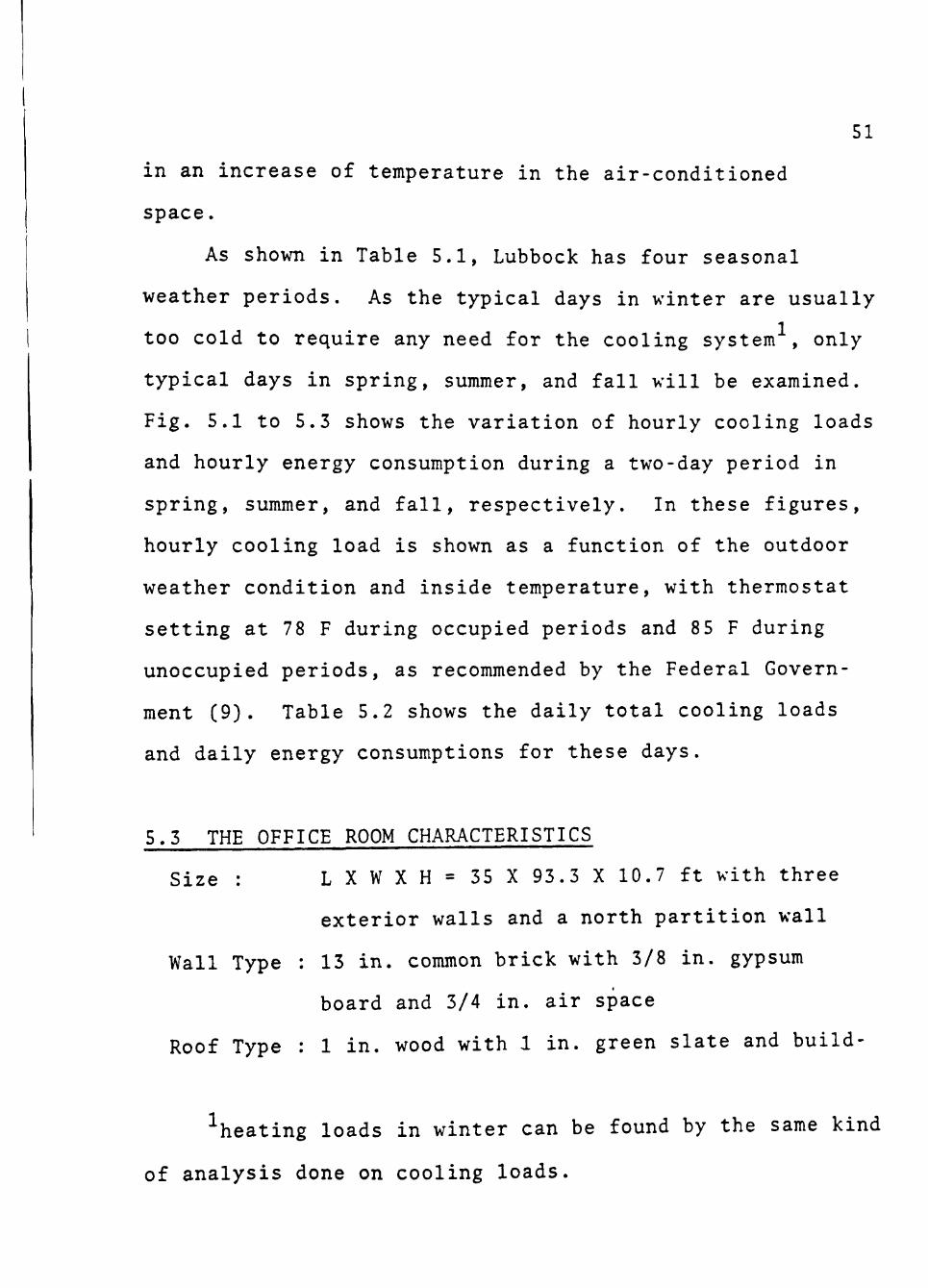
As shown in Table 5.1, Lubbock has four seasonal
weather periods. As the typical days in winter are usually
too cold to require any need for the cooling system , only
typical days in spring, summer, and fall will be examined.
Fig. 5.1 to 5.3 shows the variation of hourly cooling loads
and hourly energy consumption during a two-day period in
spring, summer, and fall, respectively. In these figures,
hourly cooling load is shown as a function of the outdoor
weather condition and inside temperature, with thermostat
setting at 78 F during occupied periods and 85 F during
unoccupied periods, as recommended by the Federal Govern
ment (9). Table 5.2 shows the daily total cooling loads
and daily energy consumptions for these days.
5.3 THE OFFICE ROOM CHARACTERISTICS
Size : L X W X H = 3 5 X 93.3 X 10.7 f t wi th t h r e e
exterior walls and a north partition wall
Wall Type : 13 in. common brick with 3/8 in. gypsum
board and 3/4 in. air space
Roof Type : 1 in. wood with 1 in. green slate and build-
•''heating loads in winter can be found by the same kind
of analysis done on cooling loads.

52
Table 5.2
Daily Energy Consumption for Typical Days
in Spring, Summer, and Fall
Date
May 13
May 14
June 27
June 28
Oct. 1
Oct. 2
Daily Cooling Load
(Btu)
164180
191878
536472
552178
45485
17812
Energy consumption
(KWH)
18.4
20.28
59.52
60.12
5.83
2.12
Table 5,1
Average Seasonal Temperature Variations of
Lubbock, Texas in 1961
Season
summer
fall
winter
spring
— _
Dry-Bulb Temperature (F)
75.77
58,60
39,43
60,47

53
o
X
—
PQ
a o
750 •
700 •
650
600
550 f-
500
450
400
350
^ 300
o o u
o
Cd
250
200
150
100
50
i8o
90
80
70
60
50
40
30^
inside temperature
outside temperature
8 12 16 20 24 28 32 36 40 44 48
Hours
Fig. 5.1. Hourly cooling loads on May 13-14 (spring).

750
o r-i
Btu/hr (x
^3 cd O
Dling
o u
700
650
600
550
500
450
400
350
300
250
200
150
100
U
Cd
o B H
50
0 100
90
80
70
60
50
40
30
54
s a
1 u
inside temperature
outside temperature
I . J
4 8 12 16 20 24 28 32 36 40 44 48
Hours
Fig. 5.2. Hourly cooling loads on June 27-28 (summer).

CVl
o
PQ
+-> cd >-• 0
H
750
700
650
600
550
500
450
400 'T3 cd
o h-1
•H r-i
o o u
350
300
250
200
150
100
50
0 100
90
80
70
60
50
40
30
55
J\
1 inside temperature
outside temperature
8 12 16 20 24 28 32 36 40 44 48
Hours
Fig. 5,3. Hourly cooling loads on Oct. 1-2 (fall).

56
Partition Wall Type :
Room Furnishing Structure
Glass Area and Types :
mg paper
3/4 in. gypsum board with
1/4 in. air space
Lightweight
155 ft^, 4.5 ft^, and 80 ft^
on the west, south, and east
Internal Loads :
Weekdays
Weekends
Schedule :
wall, respectively. All are
single, unshaded glass with
light Venetian blinds
Lights Equipment People
3 watt/ft^ .2 watt/ft^ 21
.6 watt/ft^ 0 watt/ft 1
Lights on at 0800 and off at
1800 hr. Occupants enter at
0800 and leave at 1800 hr.
Cooling System Capacity : 6 tons
Ventilation Requirement : 5 CFM/person
Single-story office buildings are commonly seen in
the Lubbock area. The hypothetical office room described
in this section is part of a single-story office building
which is typical of the existing buildings, and of the
ones under construction.

57
5.4 ENERGY CONSUMPTION FOR DIFFERENT CONTROL STRATEGIES
The energy minimization control strategies have been
developed in Chapter Three, and some of them can be evalu
ated by the present computer program. Using the same office
room and the weather conditions of the two typical days in
the summer of 1961 (June 27-28), energy consumptions for
each control strategy used during occupied period and un
occupied period are shown in Table 5.3 and 5.4, respectively,
Data in Table 5.3 and 5.4 are obtained with the space thermo
stat set at 85 F during unoccupied periods, and "8 F during
occupied periods, respectively. With the temperatures set
at 85 F during unoccupied periods for all the cases, the
control strategies used during occupied periods can be
compared to each other on an energy conservation basis.
Similarly, the control strategies for unoccupied periods can
be compared when the temperatures during occupied periods
are set at 78 F for all the cases.
As illustrated in Table 5.3 and 5,4, maintaining
space conditions at 78 F and 60% R.H. during occupied
period and letting space temperature to float during unoccu
pied period is the most economical combination which should
be used particularly in areas with weather conditions
similar to Lubbock. In other warmer geographical areas,
using night-setback at 85 F may be more advantageous.
By employing the data found, it is shown that using

58
Table 5.3
Energy Consumption for Different Control
Strategies during Occupied Period
Daily Cooling Load (Btu)
Energy Consumption (KWH)
June 27
June 28
June 27
June 28
Control Strategies
78 F, 60% R.H.
536472
552178
59.52
60.12
74 F, 50% R.H.
694651
711371
83.82
87.26
Table 5,4
Energy Consumption for Different Control
Strategies during Unoccupied Period
Daily Cooling Load (Btu)
Energy
Consumption (KWH)
June 2 7
June 28
June 27
June 28
Control Strategies
78 F
660131
675004
72,42
72.56
85 F
536472
552178
59,52
60.12
Temperature Floating
487941
512932
52.75
54.84

59
the most economical combination of control strategies
mentioned above can save energy consumption by 25%, when
compared to the common practice of maintaining the space
temperature at 78 F all day and night. When all the control
strategies developed in Chapter Three are used, seasonal
savings could be about one third. And thus it is worth
while to invest the money in installation of the micro
processor-based control system.

CHAPTER 6
CONCLUSION
As the impact of energy crisis is becoming a serious
problem, building owners are forced to seek more sophisti
cated energy conservation techniques other than the common
sense measures that were taken. Computer systems have
been used in some large buildings, which implemented the
more sophisticated conservation techniques so that heating
and cooling operations are done more efficiently. However,
it is not practical to use computer control in small
office buildings when cost factor is considered. The low
cost, versatile microprocessor-based system is a strong
candidate for use in small buildings in conserving energy.
A large building may also be divided into zones, each
zone being controlled by a microprocessor-based controller,
which in terms, are controlled by a host microprocessor.
In this thesis, a complete energy analysis of an air-
conditioned space has been done in Chapter Two. A computer
program has been written to calculate hourly energy consump
tion, and the simulation results of an office room example
is given in Chapter Five. Some of the control strategies
developed in Chapter Three can be tested by the program to
verify the amount of energy saved. These control
60

61
strategies can reduce yearly operating costs of building
cooling systems by about one third. The hardware organi
zation and the software control subroutines of the control
system are introduced in Chapter Four.
The control strategies developed in this thesis
involved the whole space under control. Further research
is needed to develop optimization control strategies for
specific groups of equipment so that the maximum efficiency
of each equipment can be fully utilized. Future research
may be directed towards using microprocessor-based control
system in large buildings.
With the continued decreasing of hardware costs, it
is likely in the future that microprocessor-based control
systems can be afforded in general residential homes.

REFERENCES
1. "Pattern of Energy Consumption in The United States," Stanford Research Institute Report, pp, 6-7.
2. "Tips for Energy Savers," Federal Energy Administration, and Energy Research and Developement Administration, Aug. 1977, pp, 8,
3. James Y, Shih, "Automation System with Addressable Sensing Devices," ASHRAE Transactions, Vol. 83, Part I, 1977, pp, 393-397.
4. "Algorithms for Calculating Transient Heat Conduction by Thermal Response Factors for Multi-Layer Structures of Various Heat Conduction Systems", National Bureau of Standards, Report # 10108,
5. D. G. Stephenson, and G, P, Mitalas, "Calculation of Heat Conduction Transfer Functions for Multi-Layer Slabs," ASHRAE Transactions, Vol. 77, Part II, 1971,
6. D. J. Vild, "Solar Heat Gain Factors and Shading Coefficients," ASHRAE Journal, Oct. 1964, pp. 47.
7. "Infiltration and Natural Ventilation," Chapter 19, ASHRAE Handbook of Fundamentals, American Society of Heating, Refrigeration, and Air-Conditioning Engineers, Inc., N,Y,, 1972, pp, 333-346.
8. D. H. Spethmann, "The Importance of Control in Energy Conservation," ASHRAE Journal, Vol. 17, No, 8, Feb, 1975, pp, 35-41.
9. "Guidelines for Saving Energy in Existing Buildings," U,S. Federal Energy Administration, June, 1975, pp. 159-161.
10. K. Kimura, and D. G. Stephenson, "Solar Radiation on Cloudy Days," ASHRAE Transactions, pp. 227-233, Part I, 1969,
11. T, Kusuda, "Algorithms for Psychrometric Calculations," Building Science Series 21, National Bureau of Standards, Jan. 1970,
62

63
12. "Air-Conditioning Cooling Load," Chapter 22, ASHRAE Handbook of Fundamentals, American Society of Heating, Refrigeration, and Air-Conditioning Engineers, Inc, N.Y., PP, 305-444, 1972,
13. C. S. Allio, "Practical Applications of Computer-Controlled Systems," ASHRAE Transactions, Vol. 80, Part I, 1974, PP. 407-408.
14. L. W. Nelson, and J. R. Tobias, "Studies of Control Applications for Energy Conservation," ASHRAE Transactions, Vol. 80, Part I, 1974, PP. 424-435.
15. A, Osborne, "An Introduction to Microcomputers Volume II--Some Real Products," Adam Osbornes and Associates, Inc,, 1976, pp. 14,1-14.24.
16. G. P. Mitalas, and J. G. Arseneault, "Fortran IV Program to Calculate z-Transform for the Calculation of Transient Heat Transfer Through Walls and Roofs," Proceedings of the first symposium on the Use of Computers for Environmental Engineering, Sept. 1971, pp. 633-668 .

APPENDIX
A-1 NOMENCLATURE OF CHAPTER TWO
a
T
"J
1. - 1 J - 1
air 03 amb
'R
p air
'p water
'p mix
^i
F. i,k
H. 1
N R
N A.CH
Absorptivity of surface
Transmissivity of glass
th Thermal diffusivity of the i surface
Final value of 1 at outside surface
Thickness of the j layer of a surface
Initial value of 1 = 0 at inside surface
Density of air
Humidity ratio of ambient air
Common ratio of transfer functions
Specific heat of air
Specific heat of water vapor
Specific heat of moisted air
Emisivity of the i surface
Radiation heat exchange view factor between
the i^ surface and k surface
: Inside surface convection heat transfer
coefficient for the i surface
: Total radiation on a surface, per unit area
: Number of nonzero terms in transfer function
relationship
: Number of air changes per hour
64

65
amb
Q ^eq
Q ^eqx
^eq,sch
^glass
Qinf
Qlite
Qlitx
^li,sch
Q ^occs
^occl
^occ.sch
%i
Q. •OS
^air
Re» ^i> ^0
3
: Pressure of ambient air
: Heat gain from equipment
: Maximum energy output of the equipment
per hour
Equipment use schedule
Heat gain due to glass area
Heat gain due to infiltration
Heat gain from lights
Maximum energy output of lights per hour
Lighting schedule
Sensible heat gain from occupants
Latent heat gain from occupants
Occupancy schedule
Latent heat generated from an adult
Sensible heat generated from an adult
Gas constant of air
Fractions of heat gain from equipment,
lights, and occupants which can be assumed
to be convective
: Temperature of outside surface
: Temperature of air in the space
: Temperature of the inside surface
: Temperature of the j^ layer of the wall
: Outside air temperature

66 T si • Inside surface temperature at the
..th surface
'^s,in,i» '^s,out,i * ^^^ide and outside surface tempera
ture history of a surface i
V : Volume of the space
^glass • Overall heat transfer coefficient
of the glass material
^f^*"^ : Transfer functions
^'» ^*» Z' : Modified transfer functions
^o • Surface heat transfer coefficient
" sa • ^ss flow rate of supply air
"^air ' ^^^ ^^0^ ^^® 0^ infiltrating air
^j • Heat flow leaving the outside surface
^in 1' ^out 1 * ^^^^ fluxes conducted in and out of
the surface in the previous hour
^sun ' Solar energy absorbed by outside wall
QQ : Heat flow going into the inside surface
A-2 MULTIPLICATION SUBROUTINE (MULT)
Binary multiplication of two 16-bit numbers produces
a 32-bit result. The calculating procedure used is the
usual add-and-shift technique. This subroutine multiplies
the value in AC2 (multiplicand) by the value in AGO
(multiplier) and provides a result in AGO (high order) and

67
ACl Clo^ order). The flow chart is shown in Fig. A.l.
MJLT
il Set loop ind^ counter
AC? = 16
Shift ACl., c-- carry
Shift carry->ACO
:>/_
Shift ACO^j-^carry
YES
ACl + AC2->AC1
Shift AGO,ACl ^left by 1 bit
AC3 - 1-^AC3
AGO + carry -^ACO
^ES
RET
Fig. A.2. Multiplication Subroutine (MULT)

68
A-3 DIVISION SUBROUTINE (DIV
Binary division is done similar to the pencil and
paper method of division. The divisor in AC2 is compared
with appropriate orders of the dividend in ACl and a
subtraction is executed only when the comparison indicates
the remainder will be positive. Result of division is
stored in ACl. The flow chart is shown in Fig. A.2.
DIV
:L Set loop in dex counter AC3 = 16
<r
Shift ACI25—>carry
Shift carry-^ACO^
AC3 - 1-^AC3
ACl + l-^ACl
/fT
>^ACO - AC2 AGO
AC3 = AC3
YES
RET
Fig. A.3. Division Subroutine iHlY)

69
A-4 TRUNCATION SUBROUTINE (TRCS)
For the interpolation calculations performed in the
enthalpy control subroutine, the 32-bit product obtained
from multiplication of a temperature difference to an
enthalpy value will be shortened to a 16-bit result by
truncating some insignificant bits. As the largest
possible value of all the products from these multipli
cations will only have 18 bits, it is a waste of memory
space and a loss of execution speed to keep every product
in two memory locations. The truncation will be done
by shifting the whole number to the left by 14 bits and
the most least significant two bits will be truncated.
The flow chart is shown in Fig. A.3.
TRCS
Shift ACl right by 2 bits
± •Shift AGO l e f t by 14 b i t s
^AC0+AC1->AC0
RET
F i g . A.4 T r u n c a t i o n Subrou t ine CTRCS)

70
A-5 SEARCH SUBROUTINE (SEARCH)
This subroutine is used to search for an entry of a
two-dimensional table providing that both the row coordin
ate (R^) and column coordinate (C ) for this particular
entry are available. The table will be arranged in memory
in the order : C^. R^. C^, R^, c^, R^, •••, c^, R^_^,
C^, RQ, ''*• The displacement from the start of the table
storage area is given by :
D = (C) (m) + R
where
C : column number (beginning with 0)
m : number of rows
R : row number (beginning with 0).
The flow chart is shown in Fig. A.5.
A-6 INTERPOLATION SUBROUTINE (INTER)
Interpolation scheme is used in the enthalpy control
subroutine to calculate corresponding enthalpy of wet-
bulb temperatures not included in the enthalpy table.
The formula which can always be used to calculate these
enthalpy is :
E = EQ (WB^ - WB) / 5 + E^ (WB - WB^) / 5
where
WB : input wet-bulb temperature

f SEARCH j
yf .
Set column no, counter N = 0
>'
Set row no.
counter L = C
71
SA : starting address
AR : address register
YES
Call MULT to get (m)(C^O
SA + (m) (Cj O + R^-^AR
RET
Fig. A.5. Search Subroutine (SEARCH)

WB , WB- : the two consecutive coordinates, which the 0 1
value of WB falls in between
E : enthalpy corresponding to WB
E. : enthalpy corresponding to WB-
The flow chart is given in Fig, A.6.
A-7 APPROXIMATION SUBROUTINE (APPROX)
This subroutine approximates a fractional number to
a whole integer value. In order to use the two tables,
dry-bulb temperature input is integerized by dividing
its value by 10 and neglecting the remainder. The flow
chart of this subroutine is very straightforward and
will be omitted here.

INTER 73
WB -WBX-^K
YES
Call SEARCH to get EQ
Call MULT to get (5 - K)E,
WBX + 5->WBX Call TRCS
WBX + 5-vWBX
WBX : minimum value on
the WB coordinate
Call DIV to get E
Call SEARCH to get E^
Call MULT to get (K)(Ei)
Call TRCS
RET
Fig. A.6. Interpolation Subroutine (INTER)