IPN Progress Report 42-159 November 15, 2004

Control and Pointing Challenges of Antennasand (Radio) Telescopes

W. Gawronski1

Extremely large telescopes will be constructed in the near future, and new radiotelescopes will operate at significantly higher radio frequencies; both features createsignificantly increased pointing-accuracy requirements that have to be addressedby control system engineers. This article presents control and pointing problemsencountered during design, testing, and operation of antennas, radio telescopes,and optical telescopes. This collection of challenges provides information on theircurrent status, helps to evaluate their importance, and is a basis for discussion onways to improve antenna pointing accuracy.

I. Introduction

In this article, we present pointing and control challenges that new antennas, radio telescopes, andoptical telescopes will meet. Radio telescopes perform operations at radio frequencies lower than opticaltelescopes. They use parabolic dishes rather than mirrors. The dish size is larger (up to 100 m) thanmirrors of optical telescopes (up to 10 m). Antennas are radio telescopes that not only can receiveradio frequency signals but also can send them. They are used for spacecraft communication. The newlydesigned antennas, radio telescopes, and telescopes have to satisfy control and pointing requirements thatchallenge existing technology. In order to increase the data rate, the antennas are required to communicateat higher radio frequencies: from S-band (2.3 GHz), to X-band, (8.5 GHz), to Ka-band (32 GHz). Theincreased frequency requires more precise pointing: 28 mdeg for S-band, 8 mdeg for X-band, and 2 mdegfor Ka-band. The telescope size also increases, from the 12-m Keck Telescope to the 30- or 50-m futuretelescopes now on drawing boards. The increased size creates multiple pointing and control challenges.

II. Antenna and Telescope Examples

A. NASA Deep Space Network

The NASA Deep Space Network (DSN) antennas communicate with spacecraft by sending commands(uplink) and by receiving information from spacecraft (downlink). To assure continuous tracking duringEarth rotation, the antennas are located at three sites: Goldstone (California), Madrid (Spain), andCanberra (Australia). The signal frequencies are 8.5 GHz (X-band) and 32 GHz (Ka-band). The dishsize of the antennas is either 34 m or 70 m. An example of a 70-m antenna is shown in Fig. 1. The

1 Communications Ground Systems Section.

The research described in this publication was carried out by the Jet Propulsion Laboratory, California Institute ofTechnology, under a contract with the National Aeronautics and Space Administration.

1

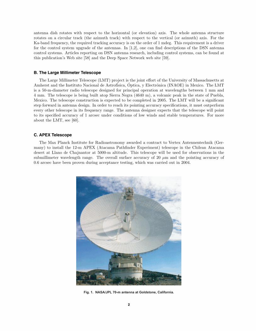
antenna dish rotates with respect to the horizontal (or elevation) axis. The whole antenna structurerotates on a circular track (the azimuth track) with respect to the vertical (or azimuth) axis. For theKa-band frequency, the required tracking accuracy is on the order of 1 mdeg. This requirement is a driverfor the control system upgrade of the antennas. In [1,2], one can find descriptions of the DSN antennacontrol systems. Articles reporting on DSN antenna research, including control systems, can be found atthis publication’s Web site [58] and the Deep Space Network web site [59].

B. The Large Millimeter Telescope

The Large Millimeter Telescope (LMT) project is the joint effort of the University of Massachusetts atAmherst and the Instituto Nacional de Astrofisica, Optica, y Electronica (INAOE) in Mexico. The LMTis a 50-m-diameter radio telescope designed for principal operation at wavelengths between 1 mm and4 mm. The telescope is being built atop Sierra Negra (4640 m), a volcanic peak in the state of Puebla,Mexico. The telescope construction is expected to be completed in 2005. The LMT will be a significantstep forward in antenna design. In order to reach its pointing accuracy specifications, it must outperformevery other telescope in its frequency range. The antenna designer expects that the telescope will pointto its specified accuracy of 1 arcsec under conditions of low winds and stable temperatures. For moreabout the LMT, see [60].

C. APEX Telescope

The Max Planck Institute for Radioastronomy awarded a contract to Vertex Antennentechnik (Ger-many) to install the 12-m APEX (Atacama Pathfinder Experiment) telescope in the Chilean Atacamadesert at Llano de Chajnantor at 5000-m altitude. This telescope will be used for observations in thesubmillimeter wavelength range. The overall surface accuracy of 20 µm and the pointing accuracy of0.6 arcsec have been proven during acceptance testing, which was carried out in 2004.

Fig. 1. NASA/JPL 70-m antenna at Goldstone, California.

2

D. ESA Deep Space Antennas

For use in deep space, high elliptical orbit missions, and future missions to Mars, the European SpaceAgency (ESA) procured 35-m deep-space ground stations. The antennas are designed for frequencies upto 35 GHz and a pointing accuracy of 6 mdeg. The first antenna has been installed in Australia andhas proven its compliance to the specifications. The second antenna is under construction in Spain. The35-m antenna incorporates a full-motion pedestal with a beam-waveguide system.

E. ALMA Prototype

The Atacama Large Millimeter Array (ALMA) has been successfully installed and tested by Vertex; abrief description can be found at [61]. The pointing accuracy of the 12-m ALMA telescope is 0.6 arcsec.The control system must handle very accurate movement at sidereal tracking velocities as well as severalextremely fast switching functions. To do this, the drives are designed to accelerate up to 24 deg/s2,which is very unusual for a telescope of this size.

F. The Thirty Meter Telescope

The Thirty Meter Telescope (TMT) will be the first of the giant optical/infrared ground-based tele-scopes addressing these compelling areas in astrophysics: the nature of dark matter and dark energy, theassembly of galaxies, the growth of structure in the universe, the physical processes involved in star andplanet formation, and the characterization of extra-solar planets. The TMT will operate over a 0.3- to30-µm wavelength range, providing 9 times the collecting area of the current largest optical telescope,the 10-m Keck Telescope. It will use an adaptive optics system to allow diffraction-limited performance,resulting in spatial resolution 12.5 times sharper than is achieved by the Hubble Space Telescope. Formore about the TMT, see [62].

G. The Multiple Mirror Telescope

The Multiple Mirror Telescope (MMT) is a joint project of the University of Arizona and the Smith-sonian Institution. Located on Mount Hopkins, Arizona, the MMT is a 6.5-m optical telescope used forspectroscopy, wide-field imaging, and adaptive optics astronomy.

Several advances in telescope design were pioneered at the MMT. Among these are a compact, altitude–azimuth structure with a co-rotating building, in-situ aluminization of the primary mirror, and adaptiveoptics with deformable secondary mirrors and artificial guide stars.

The MMT was first designed as a multiple-mirror telescope, with six 1.8-m primary mirrors in a singlemount. Automated alignment of the individual light paths gave the telescope an equivalent aperture of4.5 m, with a 6.9-m baseline for interferometry. The recent upgrade created a new 6.5-m-class telescope,although significant challenges remain in improving the telescope performance in pointing and tracking,because the structural behavior of the new telescope is not completely understood and the control systemis in the process of being re-designed. (See the MMT web site [63].)

III. Control System Structure

A typical antenna is moved in the azimuth (vertical) axis and the elevation (horizontal) axis. Themovements are independent, and their control systems are independent as well. Due to the independence,in the following we will consider a single axis only.

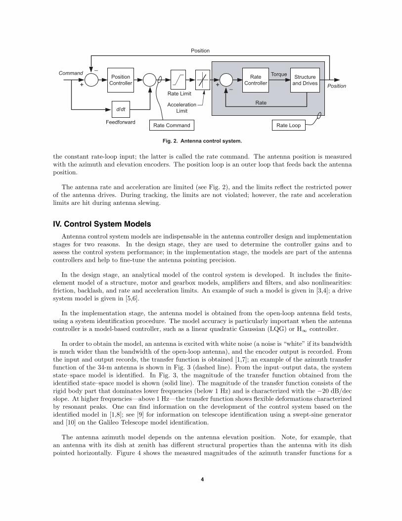
An antenna control system consists of the rate and position feedback loops, as shown in Fig. 2. Therate loop includes the antenna structure and the drives. The drive (motor) rate is fed back to the ratecontroller. Typically, the rate loop is designed such that the antenna steady-state rate is proportional to

3

Command

Position

Position

Acceleration

Limit

Torque

Rate Limit

Feedforward

Position

Controller

Rate

Controller

Rate LoopRate Command

Structure

and Drives

d/dt

+

-

+

Rate

Fig. 2. Antenna control system.

-

the constant rate-loop input; the latter is called the rate command. The antenna position is measuredwith the azimuth and elevation encoders. The position loop is an outer loop that feeds back the antennaposition.

The antenna rate and acceleration are limited (see Fig. 2), and the limits reflect the restricted powerof the antenna drives. During tracking, the limits are not violated; however, the rate and accelerationlimits are hit during antenna slewing.

IV. Control System Models

Antenna control system models are indispensable in the antenna controller design and implementationstages for two reasons. In the design stage, they are used to determine the controller gains and toassess the control system performance; in the implementation stage, the models are part of the antennacontrollers and help to fine-tune the antenna pointing precision.

In the design stage, an analytical model of the control system is developed. It includes the finite-element model of a structure, motor and gearbox models, amplifiers and filters, and also nonlinearities:friction, backlash, and rate and acceleration limits. An example of such a model is given in [3,4]; a drivesystem model is given in [5,6].

In the implementation stage, the antenna model is obtained from the open-loop antenna field tests,using a system identification procedure. The model accuracy is particularly important when the antennacontroller is a model-based controller, such as a linear quadratic Gaussian (LQG) or H∞ controller.

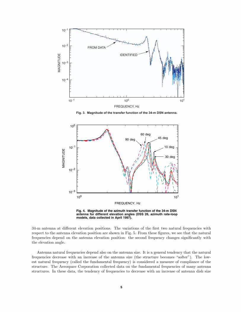
In order to obtain the model, an antenna is excited with white noise (a noise is “white” if its bandwidthis much wider than the bandwidth of the open-loop antenna), and the encoder output is recorded. Fromthe input and output records, the transfer function is obtained [1,7]; an example of the azimuth transferfunction of the 34-m antenna is shown in Fig. 3 (dashed line). From the input–output data, the systemstate–space model is identified. In Fig. 3, the magnitude of the transfer function obtained from theidentified state–space model is shown (solid line). The magnitude of the transfer function consists of therigid body part that dominates lower frequencies (below 1 Hz) and is characterized with the −20 dB/decslope. At higher frequencies—above 1 Hz—the transfer function shows flexible deformations characterizedby resonant peaks. One can find information on the development of the control system based on theidentified model in [1,8]; see [9] for information on telescope identification using a swept-sine generatorand [10] on the Galileo Telescope model identification.

The antenna azimuth model depends on the antenna elevation position. Note, for example, thatan antenna with its dish at zenith has different structural properties than the antenna with its dishpointed horizontally. Figure 4 shows the measured magnitudes of the azimuth transfer functions for a

4

10-2

10-1

10-3

10-4

FREQUENCY, Hz

FROM DATA

IDENTIFIED

10010-1 101

MA

GN

ITU

DE

Fig. 3. Magnitude of the transfer function of the 34-m DSN antenna.

90 deg

60 deg45 deg

10 deg

30 deg

MA

GN

ITU

DE

100

10−1

10−2

10−3

FREQUENCY, Hz

100 101

Fig. 4. Magnitude of the azimuth transfer function of the 34-m DSNantenna for different elevation angles (DSS 26, azimuth rate-loopmodels, data collected in April 1997).

34-m antenna at different elevation positions. The variations of the first two natural frequencies withrespect to the antenna elevation position are shown in Fig. 5. From these figures, we see that the naturalfrequencies depend on the antenna elevation position: the second frequency changes significantly withthe elevation angle.

Antenna natural frequencies depend also on the antenna size. It is a general tendency that the naturalfrequencies decrease with an increase of the antenna size (the structure becomes “softer”). The low-est natural frequency (called the fundamental frequency) is considered a measure of compliance of thestructure. The Aerospace Corporation collected data on the fundamental frequencies of many antennastructures. In these data, the tendency of frequencies to decrease with an increase of antenna dish size

5

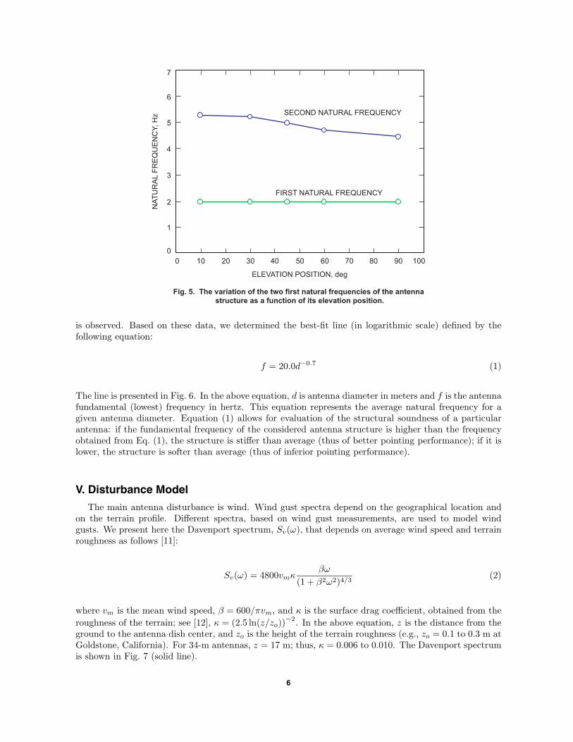
Fig. 5. The variation of the two first natural frequencies of the antenna

structure as a function of its elevation position.

7

6

5

4

3

2

1

0

0 20 40 10030 50 60 70 80 9010

NA

TU

RA

L F

RE

QU

EN

CY, H

z

ELEVATION POSITION, deg

SECOND NATURAL FREQUENCY

FIRST NATURAL FREQUENCY

is observed. Based on these data, we determined the best-fit line (in logarithmic scale) defined by thefollowing equation:

f = 20.0d−0.7 (1)

The line is presented in Fig. 6. In the above equation, d is antenna diameter in meters and f is the antennafundamental (lowest) frequency in hertz. This equation represents the average natural frequency for agiven antenna diameter. Equation (1) allows for evaluation of the structural soundness of a particularantenna: if the fundamental frequency of the considered antenna structure is higher than the frequencyobtained from Eq. (1), the structure is stiffer than average (thus of better pointing performance); if it islower, the structure is softer than average (thus of inferior pointing performance).

V. Disturbance Model

The main antenna disturbance is wind. Wind gust spectra depend on the geographical location andon the terrain profile. Different spectra, based on wind gust measurements, are used to model windgusts. We present here the Davenport spectrum, Sv(ω), that depends on average wind speed and terrainroughness as follows [11]:

Sv(ω) = 4800vmκβω

(1 + β2ω2)4/3(2)

where vm is the mean wind speed, β = 600/πvm, and κ is the surface drag coefficient, obtained from theroughness of the terrain; see [12], κ = (2.5 ln(z/zo))

−2. In the above equation, z is the distance from theground to the antenna dish center, and zo is the height of the terrain roughness (e.g., zo = 0.1 to 0.3 m atGoldstone, California). For 34-m antennas, z = 17 m; thus, κ = 0.006 to 0.010. The Davenport spectrumis shown in Fig. 7 (solid line).

6

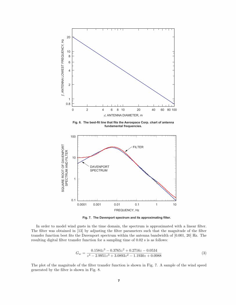
Fig. 6. The best-fit line that fits the Aerospace Corp. chart of antenna

fundamental frequencies.

20

6

4

2

10

8

1

0.8

0 20 40 1004 10 60 802 86

ƒ, A

NT

EN

NA

LO

WE

ST

FR

EQ

UE

NC

Y, H

z

d, ANTENNA DIAMETER, m

FILTER

DAVENPORT

SPECTRUM

FREQUENCY, Hz

100

10

1

0.1

0.0001 0.001 0.01 0.1 101

SQ

UA

RE

RO

OT

OF

DA

VE

NP

OR

T

SP

EC

TR

UM

AN

D F

ILT

ER

Fig. 7. The Davenport spectrum and its approximating filter.

In order to model wind gusts in the time domain, the spectrum is approximated with a linear filter.The filter was obtained in [13] by adjusting the filter parameters such that the magnitude of the filtertransfer function best fits the Davenport spectrum within the antenna bandwidth of [0.001, 20] Hz. Theresulting digital filter transfer function for a sampling time of 0.02 s is as follows:

Gw =0.1584z3 − 0.3765z2 + 0.2716z − 0.0534

z4 − 2.9951z3 + 3.0893z2 − 1.1930z + 0.0988(3)

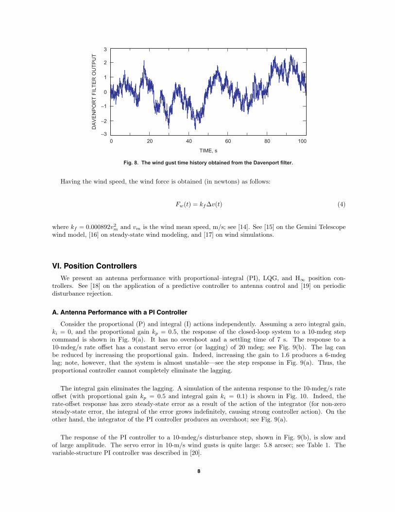
The plot of the magnitude of the filter transfer function is shown in Fig. 7. A sample of the wind speedgenerated by the filter is shown in Fig. 8.

7

0 20 40

TIME, s

Fig. 8. The wind gust time history obtained from the Davenport filter.

DA

VE

NP

OR

T F

ILT

ER

OU

TP

UT

60 80 100

-3

-2

-1

0

1

2

3

Having the wind speed, the wind force is obtained (in newtons) as follows:

Fw(t) = kf∆v(t) (4)

where kf = 0.000892v2m and vm is the wind mean speed, m/s; see [14]. See [15] on the Gemini Telescope

wind model, [16] on steady-state wind modeling, and [17] on wind simulations.

VI. Position Controllers

We present an antenna performance with proportional–integral (PI), LQG, and H∞ position con-trollers. See [18] on the application of a predictive controller to antenna control and [19] on periodicdisturbance rejection.

A. Antenna Performance with a PI Controller

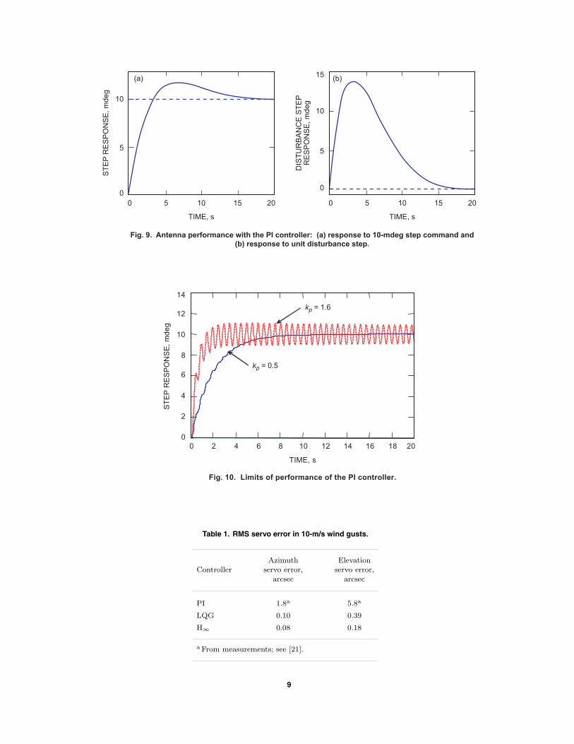
Consider the proportional (P) and integral (I) actions independently. Assuming a zero integral gain,ki = 0, and the proportional gain kp = 0.5, the response of the closed-loop system to a 10-mdeg stepcommand is shown in Fig. 9(a). It has no overshoot and a settling time of 7 s. The response to a10-mdeg/s rate offset has a constant servo error (or lagging) of 20 mdeg; see Fig. 9(b). The lag canbe reduced by increasing the proportional gain. Indeed, increasing the gain to 1.6 produces a 6-mdeglag; note, however, that the system is almost unstable—see the step response in Fig. 9(a). Thus, theproportional controller cannot completely eliminate the lagging.

The integral gain eliminates the lagging. A simulation of the antenna response to the 10-mdeg/s rateoffset (with proportional gain kp = 0.5 and integral gain ki = 0.1) is shown in Fig. 10. Indeed, therate-offset response has zero steady-state error as a result of the action of the integrator (for non-zerosteady-state error, the integral of the error grows indefinitely, causing strong controller action). On theother hand, the integrator of the PI controller produces an overshoot; see Fig. 9(a).

The response of the PI controller to a 10-mdeg/s disturbance step, shown in Fig. 9(b), is slow andof large amplitude. The servo error in 10-m/s wind gusts is quite large: 5.8 arcsec; see Table 1. Thevariable-structure PI controller was described in [20].

8

10

0 5 1510

TIME, s

20

5

0

0 5 1510

TIME, s

20

ST

EP

RE

SP

ON

SE

, m

deg

10

15

5

0

DIS

TU

RB

AN

CE

ST

EP

RE

SP

ON

SE

, m

deg

(a) (b)

Fig. 9. Antenna performance with the PI controller: (a) response to 10-mdeg step command and

(b) response to unit disturbance step.

0 2 4 6 8 10

TIME, s

12 14 16 18 20

0

2

4

6

8

10

12

14

kp = 1.6

kp = 0.5

ST

EP

RE

SP

ON

SE

, m

deg

Fig. 10. Limits of performance of the PI controller.

Table 1. RMS servo error in 10-m/s wind gusts.

Azimuth ElevationController servo error, servo error,

arcsec arcsec

PI 1.8a 5.8a

LQG 0.10 0.39

H∞ 0.08 0.18

a From measurements; see [21].

9

B. Antenna Performance with a Feedforward Controller

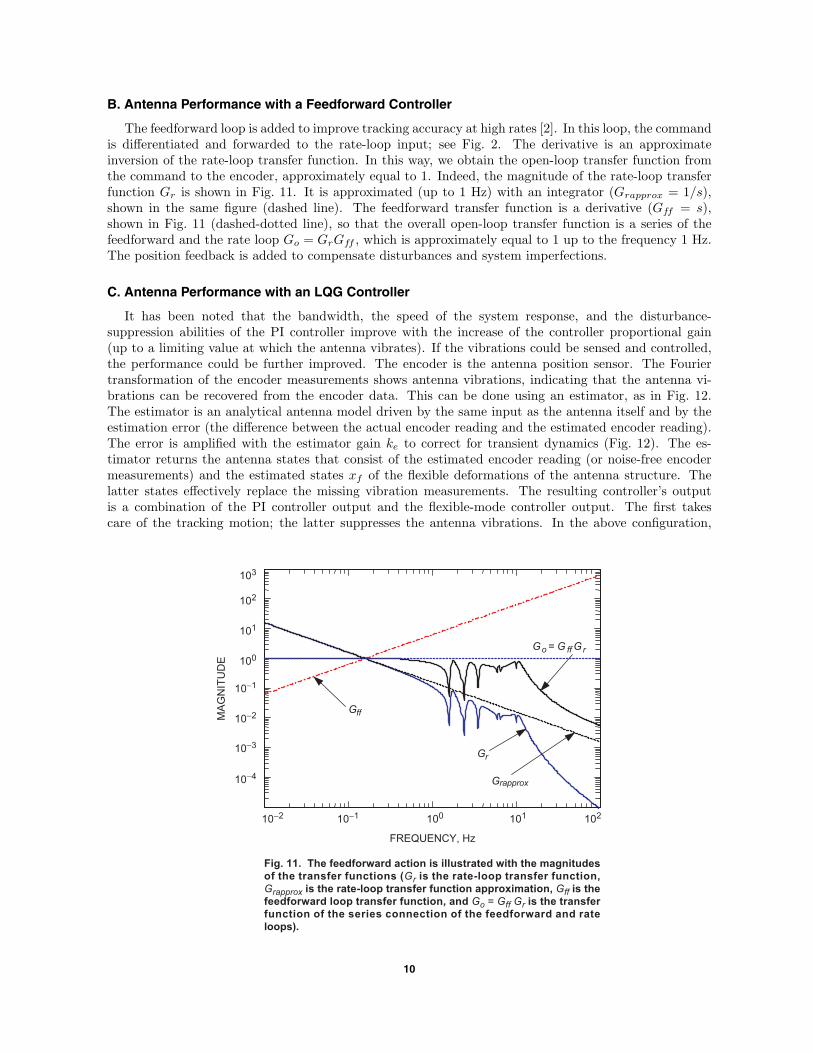
The feedforward loop is added to improve tracking accuracy at high rates [2]. In this loop, the commandis differentiated and forwarded to the rate-loop input; see Fig. 2. The derivative is an approximateinversion of the rate-loop transfer function. In this way, we obtain the open-loop transfer function fromthe command to the encoder, approximately equal to 1. Indeed, the magnitude of the rate-loop transferfunction Gr is shown in Fig. 11. It is approximated (up to 1 Hz) with an integrator (Grapprox = 1/s),shown in the same figure (dashed line). The feedforward transfer function is a derivative (Gff = s),shown in Fig. 11 (dashed-dotted line), so that the overall open-loop transfer function is a series of thefeedforward and the rate loop Go = GrGff , which is approximately equal to 1 up to the frequency 1 Hz.The position feedback is added to compensate disturbances and system imperfections.

C. Antenna Performance with an LQG Controller

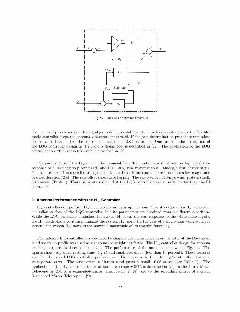
It has been noted that the bandwidth, the speed of the system response, and the disturbance-suppression abilities of the PI controller improve with the increase of the controller proportional gain(up to a limiting value at which the antenna vibrates). If the vibrations could be sensed and controlled,the performance could be further improved. The encoder is the antenna position sensor. The Fouriertransformation of the encoder measurements shows antenna vibrations, indicating that the antenna vi-brations can be recovered from the encoder data. This can be done using an estimator, as in Fig. 12.The estimator is an analytical antenna model driven by the same input as the antenna itself and by theestimation error (the difference between the actual encoder reading and the estimated encoder reading).The error is amplified with the estimator gain ke to correct for transient dynamics (Fig. 12). The es-timator returns the antenna states that consist of the estimated encoder reading (or noise-free encodermeasurements) and the estimated states xf of the flexible deformations of the antenna structure. Thelatter states effectively replace the missing vibration measurements. The resulting controller’s outputis a combination of the PI controller output and the flexible-mode controller output. The first takescare of the tracking motion; the latter suppresses the antenna vibrations. In the above configuration,

103

102

101

100

10-1

10-2

10-2 10-1 101 102100

10-3

10-4

Gff

Gr

Grapprox

Go = G ff Gr

MA

GN

ITU

DE

FREQUENCY, Hz

Fig. 11. The feedforward action is illustrated with the magnitudes

of the transfer functions (Gr is the rate-loop transfer function,

Grapprox is the rate-loop transfer function approximation, Gff is the

feedforward loop transfer function, and Go = Gff Gr is the transfer

function of the series connection of the feedforward and rate

loops).

10

++

+

_

_

+

+

Estimator

e

r e

y

x fest

yest

kf

ki

kp

uc

uc

ei

ke

Fig. 12. The LQG controller structure.

the increased proportional-and-integral gains do not destabilize the closed-loop system, since the flexible-mode controller keeps the antenna vibrations suppressed. If the gain determination procedure minimizesthe so-called LQG index, the controller is called an LQG controller. One can find the description ofthe LQG controller design in [1,7], and a design tool is described in [22]. The application of the LQGcontroller to a 20-m radio telescope is described in [23].

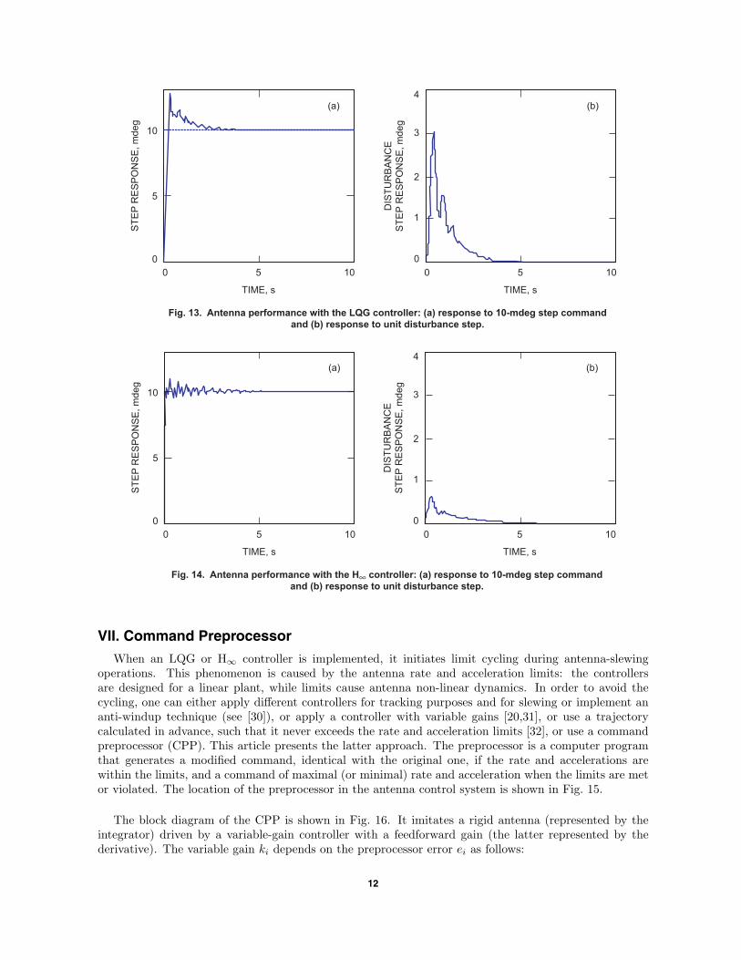
The performance of the LQG controller designed for a 34-m antenna is illustrated in Fig. 13(a) (theresponse to a 10-mdeg step command) and Fig. 13(b) (the response to a 10-mdeg/s disturbance step).The step response has a small settling time of 2 s, and the disturbance step response has a low magnitudeof short duration (2 s). The rate offset shows zero lagging. The servo error in 10-m/s wind gusts is small:0.10 arcsec (Table 1). These parameters show that the LQG controller is of an order better than the PIcontroller.

D. Antenna Performance with the H∞ Controller

H∞ controllers outperform LQG controllers in many applications. The structure of an H∞ controlleris similar to that of the LQG controller, but its parameters are obtained from a different algorithm.While the LQG controller minimizes the system H2 norm (its rms response to the white noise input),the H∞ controller algorithm minimizes the system H∞ norm (in the case of a single-input–single-outputsystem, the system H∞ norm is the maximal magnitude of its transfer function).

The antenna H∞ controller was designed by shaping the disturbance input. A filter of the Davenportwind spectrum profile was used as a shaping (or weighting) factor. The H∞ controller design for antennatracking purposes is described in [1,24]. The performance of the antenna is shown in Fig. 14. Thefigures show very small settling time (1.2 s) and small overshoot (less than 10 percent). These featuressignificantly exceed LQG controller performance. The response to the 10-mdeg/s rate offset has zerosteady-state error. The servo error in 10-m/s wind gusts is small: 0.08 arcsec (see Table 1). Theapplication of the H∞ controller to the airborne telescope SOFIA is described in [25], to the Thirty MeterTelescope in [26], to a segmented-mirror telescope in [27,28], and to the secondary mirror of a GiantSegmented Mirror Telescope in [29].

11

(a) (b)

10

5

0

0 5

TIME, s

10

ST

EP

RE

SP

ON

SE

, m

deg

3

4

2

1

0

0 5

TIME, s

10

DIS

TU

RB

AN

CE

ST

EP

RE

SP

ON

SE

, m

deg

Fig. 13. Antenna performance with the LQG controller: (a) response to 10-mdeg step command

and (b) response to unit disturbance step.

(a) (b)

10

5

0

0 5

TIME, s

10

ST

EP

RE

SP

ON

SE

, m

deg

3

4

2

1

0

0 5

TIME, s

10

DIS

TU

RB

AN

CE

ST

EP

RE

SP

ON

SE

, m

deg

Fig. 14. Antenna performance with the H• controller: (a) response to 10-mdeg step command

and (b) response to unit disturbance step.

VII. Command Preprocessor

When an LQG or H∞ controller is implemented, it initiates limit cycling during antenna-slewingoperations. This phenomenon is caused by the antenna rate and acceleration limits: the controllersare designed for a linear plant, while limits cause antenna non-linear dynamics. In order to avoid thecycling, one can either apply different controllers for tracking purposes and for slewing or implement ananti-windup technique (see [30]), or apply a controller with variable gains [20,31], or use a trajectorycalculated in advance, such that it never exceeds the rate and acceleration limits [32], or use a commandpreprocessor (CPP). This article presents the latter approach. The preprocessor is a computer programthat generates a modified command, identical with the original one, if the rate and accelerations arewithin the limits, and a command of maximal (or minimal) rate and acceleration when the limits are metor violated. The location of the preprocessor in the antenna control system is shown in Fig. 15.

The block diagram of the CPP is shown in Fig. 16. It imitates a rigid antenna (represented by theintegrator) driven by a variable-gain controller with a feedforward gain (the latter represented by thederivative). The variable gain ki depends on the preprocessor error ei as follows:

12

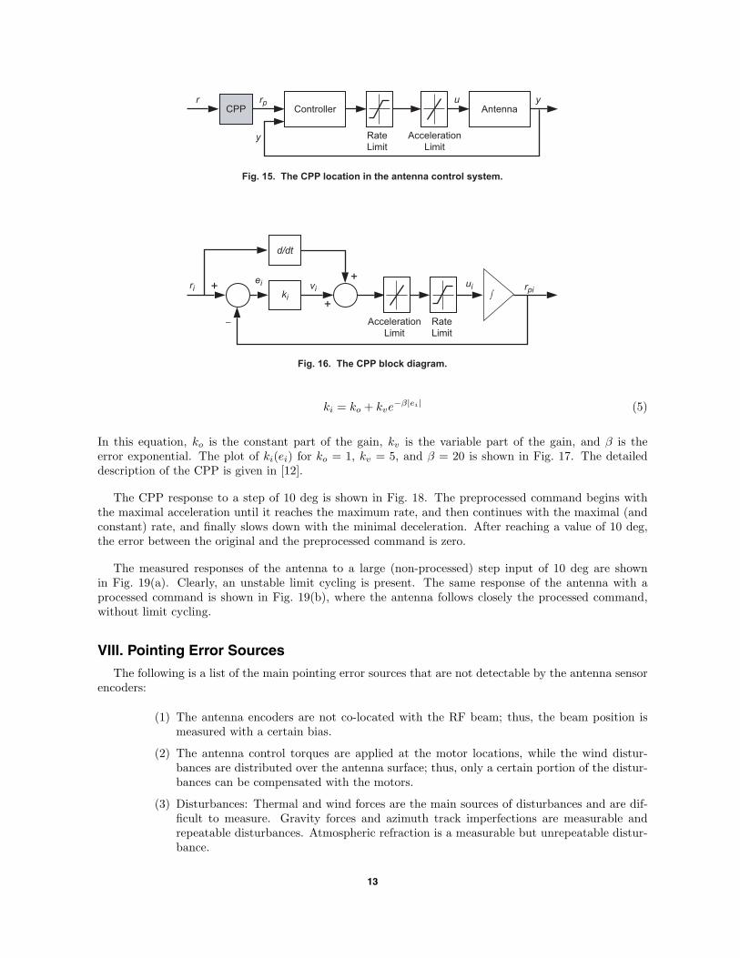
Fig. 15. The CPP location in the antenna control system.

Rate

Limit

Acceleration

Limit

r u y

y

rpController AntennaCPP

Fig. 16. The CPP block diagram.

Acceleration

Limit

Rate

Limit

ki

ri

d/dt

+

+

+ei viui rpi

-

ki = ko + kve−β|ei| (5)

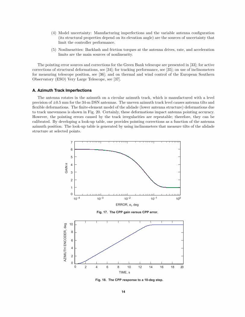
In this equation, ko is the constant part of the gain, kv is the variable part of the gain, and β is theerror exponential. The plot of ki(ei) for ko = 1, kv = 5, and β = 20 is shown in Fig. 17. The detaileddescription of the CPP is given in [12].

The CPP response to a step of 10 deg is shown in Fig. 18. The preprocessed command begins withthe maximal acceleration until it reaches the maximum rate, and then continues with the maximal (andconstant) rate, and finally slows down with the minimal deceleration. After reaching a value of 10 deg,the error between the original and the preprocessed command is zero.

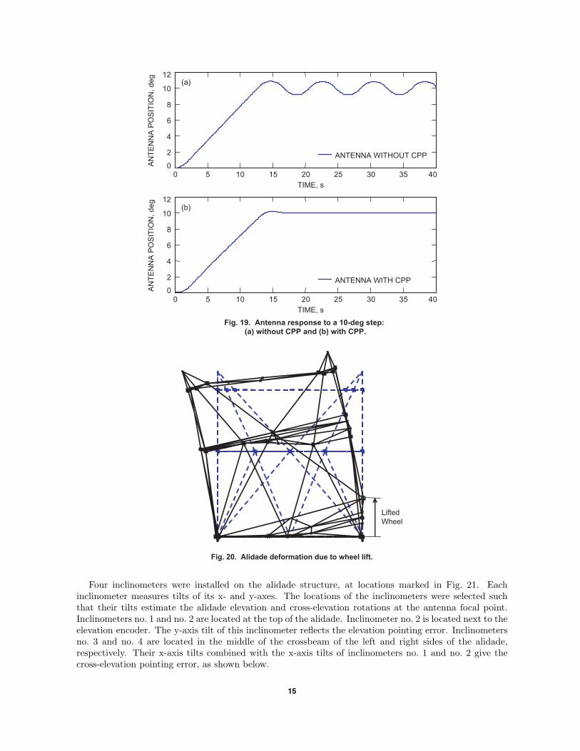
The measured responses of the antenna to a large (non-processed) step input of 10 deg are shownin Fig. 19(a). Clearly, an unstable limit cycling is present. The same response of the antenna with aprocessed command is shown in Fig. 19(b), where the antenna follows closely the processed command,without limit cycling.

VIII. Pointing Error Sources

The following is a list of the main pointing error sources that are not detectable by the antenna sensorencoders:

(1) The antenna encoders are not co-located with the RF beam; thus, the beam position ismeasured with a certain bias.

(2) The antenna control torques are applied at the motor locations, while the wind distur-bances are distributed over the antenna surface; thus, only a certain portion of the distur-bances can be compensated with the motors.

(3) Disturbances: Thermal and wind forces are the main sources of disturbances and are dif-ficult to measure. Gravity forces and azimuth track imperfections are measurable andrepeatable disturbances. Atmospheric refraction is a measurable but unrepeatable distur-bance.

13

(4) Model uncertainty: Manufacturing imperfections and the variable antenna configuration(its structural properties depend on its elevation angle) are the sources of uncertainty thatlimit the controller performance.

(5) Nonlinearities: Backlash and friction torques at the antenna drives, rate, and accelerationlimits are the main sources of nonlinearity.

The pointing error sources and corrections for the Green Bank telescope are presented in [33]; for activecorrections of structural deformations, see [34]; for tracking performance, see [35]; on use of inclinometersfor measuring telescope position, see [36]; and on thermal and wind control of the European SouthernObservatory (ESO) Very Large Telescope, see [37].

A. Azimuth Track Imperfections

The antenna rotates in the azimuth on a circular azimuth track, which is manufactured with a levelprecision of ±0.5 mm for the 34-m DSN antennas. The uneven azimuth track level causes antenna tilts andflexible deformations. The finite-element model of the alidade (lower antenna structure) deformations dueto track unevenness is shown in Fig. 20. Certainly, these deformations impact antenna pointing accuracy.However, the pointing errors caused by the track irregularities are repeatable; therefore, they can becalibrated. By developing a look-up table, one provides pointing corrections as a function of the antennaazimuth position. The look-up table is generated by using inclinometers that measure tilts of the alidadestructure at selected points.

0

1

2

3

4

5

6

7

10-4 10-3 10-2 10-1 100

GA

IN k

ERROR, ei, deg

Fig. 17. The CPP gain versus CPP error.

0 2 4 6 8 10 12 14 16 18 20

0

2

4

6

8

10

TIME, s

AZ

IMU

TH

EN

CO

DE

R,

de

g

Fig. 18. The CPP response to a 10-deg step.

14

0 5 10 15 20 25 30 35 400

2

4

6

8

10

12

ANTENNA WITHOUT CPP

TIME, s

AN

TE

NN

A P

OS

ITIO

N,

de

g

(a)

0

2

4

6

8

10

12

ANTENNA WITH CPP

0 5 10 15 20 25 30 35 40

TIME, s

AN

TE

NN

A P

OS

ITIO

N,

de

g

(b)

Fig. 19. Antenna response to a 10-deg step:

(a) without CPP and (b) with CPP.

Lifted

Wheel

Fig. 20. Alidade deformation due to wheel lift.

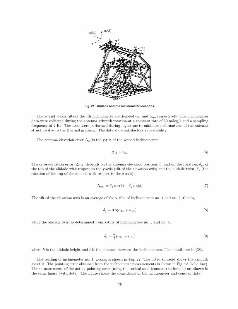
Four inclinometers were installed on the alidade structure, at locations marked in Fig. 21. Eachinclinometer measures tilts of its x- and y-axes. The locations of the inclinometers were selected suchthat their tilts estimate the alidade elevation and cross-elevation rotations at the antenna focal point.Inclinometers no. 1 and no. 2 are located at the top of the alidade. Inclinometer no. 2 is located next to theelevation encoder. The y-axis tilt of this inclinometer reflects the elevation pointing error. Inclinometersno. 3 and no. 4 are located in the middle of the crossbeam of the left and right sides of the alidade,respectively. Their x-axis tilts combined with the x-axis tilts of inclinometers no. 1 and no. 2 give thecross-elevation pointing error, as shown below.

15

x(EL)z(AZ)

y

y

xy

x

Fig. 21. Alidade and the inclinometer locations.

The x- and y-axis tilts of the ith inclinometer are denoted αix and αiy, respectively. The inclinometerdata were collected during the antenna azimuth rotation at a constant rate of 50 mdeg/s and a samplingfrequency of 2 Hz. The tests were performed during nighttime to minimize deformations of the antennastructure due to the thermal gradient. The data show satisfactory repeatability.

The antenna elevation error ∆el is the y-tilt of the second inclinometer:

∆el = α2y (6)

The cross-elevation error, ∆xel, depends on the antenna elevation position, θ, and on the rotation, δy, ofthe top of the alidade with respect to the y-axis (tilt of the elevation axis) and the alidade twist, δz (therotation of the top of the alidade with respect to the z-axis):

∆xel = δz cos(θ) − δy sin(θ) (7)

The tilt of the elevation axis is an average of the x-tilts of inclinometers no. 1 and no. 2, that is,

δy = 0.5(α1x + α2x) (8)

while the alidade twist is determined from x-tilts of inclinometers no. 3 and no. 4,

δz =h

l(α7x − α8x) (9)

where h is the alidade height and l is the distance between the inclinometers. The details are in [38].

The reading of inclinometer no. 1, x-axis, is shown in Fig. 22. The fitted sinusoid shows the azimuthaxis tilt. The pointing error obtained from the inclinometer measurements is shown in Fig. 23 (solid line).The measurements of the actual pointing error (using the conical scan (conscan) technique) are shown inthe same figure (with dots). The figure shows the coincidence of the inclinometer and conscan data.

16

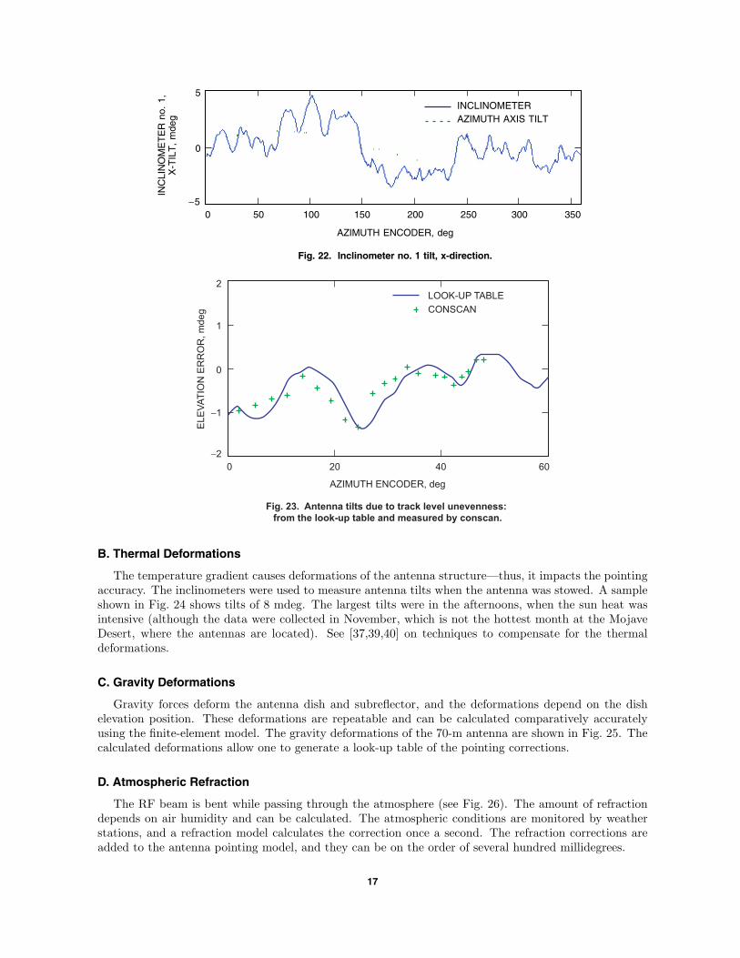
350

Fig. 22. Inclinometer no. 1 tilt, x-direction.

−5

5

0IN

CLI

NO

ME

TE

R n

o. 1

,X

-TIL

T,

mde

g

AZIMUTH ENCODER, deg

INCLINOMETERAZIMUTH AXIS TILT

300250200150100500

Fig. 23. Antenna tilts due to track level unevenness:

from the look-up table and measured by conscan.

-2

-1

2

1

0

0 20 40 60

ELE

VA

TIO

N E

RR

OR

, m

deg

AZIMUTH ENCODER, deg

LOOK-UP TABLE

CONSCAN

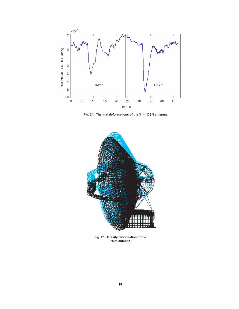
B. Thermal Deformations

The temperature gradient causes deformations of the antenna structure—thus, it impacts the pointingaccuracy. The inclinometers were used to measure antenna tilts when the antenna was stowed. A sampleshown in Fig. 24 shows tilts of 8 mdeg. The largest tilts were in the afternoons, when the sun heat wasintensive (although the data were collected in November, which is not the hottest month at the MojaveDesert, where the antennas are located). See [37,39,40] on techniques to compensate for the thermaldeformations.

C. Gravity Deformations

Gravity forces deform the antenna dish and subreflector, and the deformations depend on the dishelevation position. These deformations are repeatable and can be calculated comparatively accuratelyusing the finite-element model. The gravity deformations of the 70-m antenna are shown in Fig. 25. Thecalculated deformations allow one to generate a look-up table of the pointing corrections.

D. Atmospheric Refraction

The RF beam is bent while passing through the atmosphere (see Fig. 26). The amount of refractiondepends on air humidity and can be calculated. The atmospheric conditions are monitored by weatherstations, and a refraction model calculates the correction once a second. The refraction corrections areadded to the antenna pointing model, and they can be on the order of several hundred millidegrees.

17

0 5 10 15 20

TIME, h

INC

LIN

OM

ET

ER

TIL

T, m

deg

25 30 35 40 45

-6

-5

-4

-3

-2

-1

0

1

2

x10-3

DAY 1 DAY 2

Fig. 24. Thermal deformations of the 34-m DSN antenna.

Fig. 25. Gravity deformation of the

70-m antenna.

18

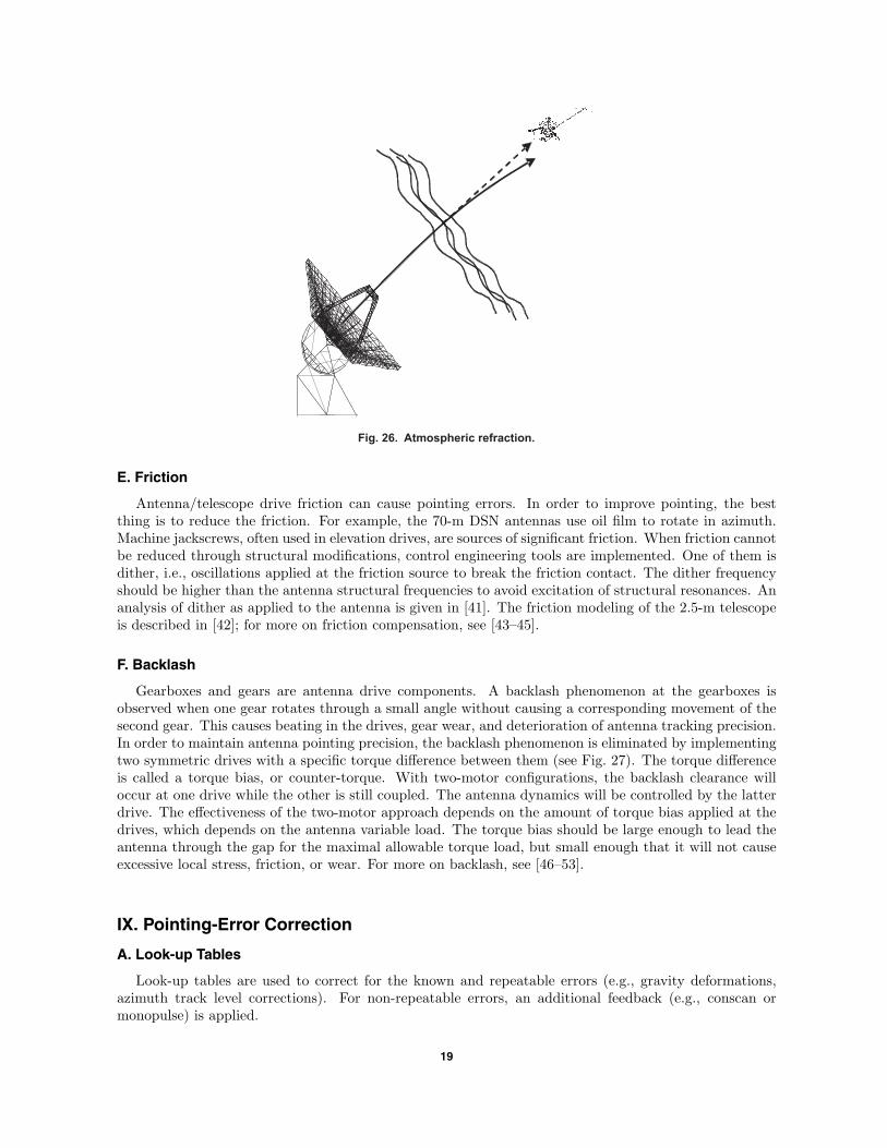
Fig. 26. Atmospheric refraction.

E. Friction

Antenna/telescope drive friction can cause pointing errors. In order to improve pointing, the bestthing is to reduce the friction. For example, the 70-m DSN antennas use oil film to rotate in azimuth.Machine jackscrews, often used in elevation drives, are sources of significant friction. When friction cannotbe reduced through structural modifications, control engineering tools are implemented. One of them isdither, i.e., oscillations applied at the friction source to break the friction contact. The dither frequencyshould be higher than the antenna structural frequencies to avoid excitation of structural resonances. Ananalysis of dither as applied to the antenna is given in [41]. The friction modeling of the 2.5-m telescopeis described in [42]; for more on friction compensation, see [43–45].

F. Backlash

Gearboxes and gears are antenna drive components. A backlash phenomenon at the gearboxes isobserved when one gear rotates through a small angle without causing a corresponding movement of thesecond gear. This causes beating in the drives, gear wear, and deterioration of antenna tracking precision.In order to maintain antenna pointing precision, the backlash phenomenon is eliminated by implementingtwo symmetric drives with a specific torque difference between them (see Fig. 27). The torque differenceis called a torque bias, or counter-torque. With two-motor configurations, the backlash clearance willoccur at one drive while the other is still coupled. The antenna dynamics will be controlled by the latterdrive. The effectiveness of the two-motor approach depends on the amount of torque bias applied at thedrives, which depends on the antenna variable load. The torque bias should be large enough to lead theantenna through the gap for the maximal allowable torque load, but small enough that it will not causeexcessive local stress, friction, or wear. For more on backlash, see [46–53].

IX. Pointing-Error Correction

A. Look-up Tables

Look-up tables are used to correct for the known and repeatable errors (e.g., gravity deformations,azimuth track level corrections). For non-repeatable errors, an additional feedback (e.g., conscan ormonopulse) is applied.

19

MOTOR 2

TORQUE BIAS

MOTOR 1

100

80

60

20

0

-20

-40

-80

-60

-100

-100 -80 -60 -40 -20 0 20

ANTENNA LOAD/MAXIMUM ANTENNA LOAD, percent

60 10040 80

40

MO

TO

R L

OA

D/M

AX

IMU

M M

OT

OR

LO

AD

, perc

ent

Fig. 27. Motor torques and the counter-torque.

MOTOR 1 + MOTOR 2 = ANTENNA LOAD

B. Conical Scan (Conscan)

Conscan is an additional feedback. This technique is commonly used for the determination of the truespacecraft position. During conscan, circular movements are added to the antenna command, as shownin Fig. 28. The circular movements cause sinusoidal variations of the power of the signal received fromthe spacecraft, as illustrated in Fig. 29. The power variations are used to estimate the true spacecraftposition. The time of one cycle is between 30 and 60 s; thus, the correction update is comparatively slow.The drawback of this technique is that the antenna is always off the peak power, i.e., always slightly offthe target.

The control system of the conscan consists of the additional (outer) feedback that corrects for thedifference between the encoder and RF beam position (see Fig. 30). For more about conscan, see [54,55].

C. Monopulse

In this algorithm, the pointing error is estimated from RF signals received by the monopulse feedhorn. These signals are uniquely related in amplitude and phase as a function of the antenna pointingerror. The single monopulse feed design allows direct pointing at the target at all times, allowing for thespacecraft to be tracked at the peak of the antenna pattern. This technique is much faster than conscan(the updating time is 0.02 s). For more about monopulse, see [56,57].

X. Conclusions

This article presented the challenges that control system engineers encounter while trying to satisfydemanding pointing requirements. Not all challenges have satisfactory solutions. One of the reasons isthe lack of a stable point of reference to measure the RF beam position. The substitute beam positionmeasurements using encoders are subject to painstaking corrections, which do not always satisfy therequirements. A fast and inexpensive measurement system of beam position would be a breakthrough inantenna/telescope technology.

20

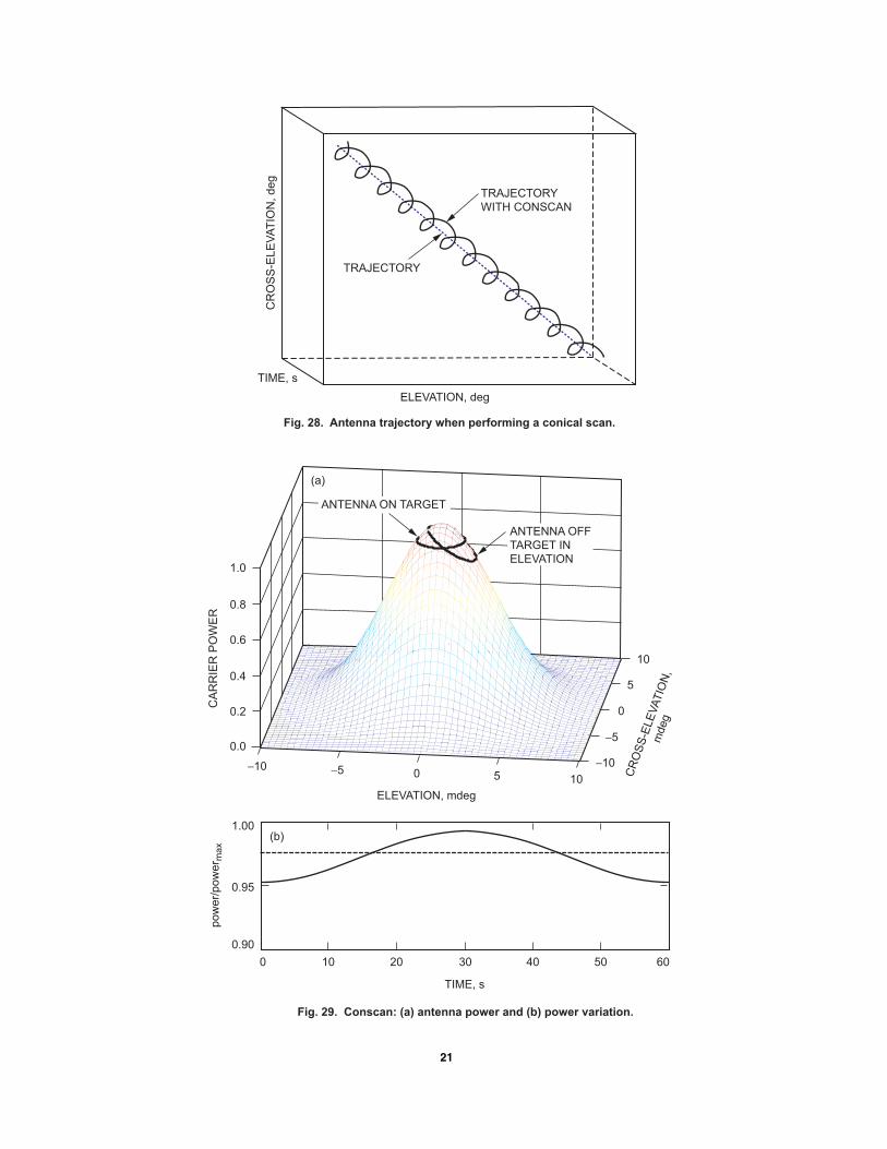
Fig. 28. Antenna trajectory when performing a conical scan.

TRAJECTORY

WITH CONSCAN

TRAJECTORYC

RO

SS

-ELE

VA

TIO

N, deg

ELEVATION, deg

TIME, s

Fig. 29. Conscan: (a) antenna power and (b) power variation.

TIME, s

10

0.95

0.90

1.00

0 20

pow

er/

pow

er m

ax

30 40 50 60

(b)

0.8

1.0

0.6

0.4

0.2

0.0

-10 -5 0

CA

RR

IER

PO

WE

R

5 10

-10

-5

0

5

10

CR

OS

S-E

LE

VA

TIO

N,

mdeg

ANTENNA ON TARGET

ELEVATION, mdeg

ANTENNA OFF

TARGET IN

ELEVATION

(a)

21

Fig. 30. Antenna conscan controller.

Conscan

Estimator

Conscan

ControllerAntenna

BeamPosition

Encoder

Command

Antenna

Controller

References

[1] W. Gawronski, Advanced Structural Dynamics, and Active Control of Structures,New York: Springer, 2004.

[2] W. Gawronski and J. A. Mellstrom, “Control and Dynamics of the Deep SpaceNetwork Antennas,” chapter in Control and Dynamic Systems, vol. 63, ed.,C. T. Leondes, San Diego, California: Academic Press, 1994.

[3] W. Gawronski and K. Souccar, “Control System of the Large Millimeter Tele-scope,” SPIE Astronomical Telescopes and Instrumentation Conference, Glas-gow, United Kingdom, June 2004.

[4] D. Clark “Control System Prototyping—A Case Study,” Technical Memoran-dum ITM-04-3, MMT Observatory, Smithsonian Institution and The Universityof Arizona, www.mmto.org/MMTpapers/tech00 10.shtml#2004

[5] T. Erm and P. Gutierrez, “Integration and Tuning of the VLT Drive Systems,”Proceedings of the SPIE, Telescope Structures, Enclosures, Controls, Assem-bly/Integration/Validation, and Commissioning, vol. 4004, 2000.

[6] S. Jimenez-Garcia, M. E. Magana, J. S. Benitez-Read, and J. Martinez-Carbalido, “Modeling, Simulation, and Gain Scheduling Control of Large Ra-diotelescopes,” Simulation Practice and Theory, vol. 8, pp. 141–160, 2000.

[7] W. Gawronski, C. Racho, and J. Mellstrom, “Application of the LQG and Feed-forward Controllers for the DSN Antennas,” IEEE Transactions on Control Sys-tems Technology, vol. 3, pp. 417–421, 1995; also seetmo.jpl.nasa.gov/tmo/progress report/42-109/109R.PDF andtmo.jpl.nasa.gov/tmo/progress report/42-112/112J.PDF

[8] W. Gawronski, H. G. Ahlstrom, and A. M. Bernardo, “Analysis and Performanceof the Control Systems of the NASA 70-Meter Antennas,” ISA Transactions,vol. 43, 2004; also seetmo.jpl.nasa.gov/tmo/progress report/42-144/144D.pdf

[9] D. Clark, “Selected Results of Recent MMT Servo Testing,” Technical Memoran-dum ITM-03-5, MMT Observatory, Smithsonian Institution and The Universityof Arizona, July 2003, www.mmto.org/MMTpapers/pdfs/itm/itm03-5.pdf

[10] E. Cascone, D. Mancini, and P. Schipani, “Galileo Telescope Model Identifica-tion,” Proceedings of the SPIE, vol. 3112, pp. 343–350, 1997.

22

[11] E. Simiu and R. H. Scanlan, Wind Effects on Structures, New York: Wiley, 1978.

[12] W. Gawronski and W. Almassy, “Command Pre-Processor for Radiotelescopesand Microwave Antennas,” IEEE Antennas and Propagation Magazine, vol. 44,no. 2, pp. 30–37, 2002; also seehtmo.jpl.nasa.gov/tmo/progress report/42-136/136A.pdf andipnpr.jpl.nasa.gov/tmo/progress report/42-150/150G.pdf

[13] W. Gawronski, B. Bienkiewicz, and R. E. Hill, “Wind-Induced Dynamics of aDeep Space Network Antenna,” Journal of Sound and Vibration, vol. 178, no. 1,pp. 67–77, 1994; also seetmo.jpl.nasa.gov/tmo/progress report/42-108/108J.PDF

[14] W. Gawronski, “Modeling Wind Gusts Disturbances for the Analysis of An-tenna Pointing Accuracy,” IEEE Antennas and Propagation Magazine, vol. 46,no. 1, pp. 50–58, 2004; also seeipnpr.jpl.nasa.gov/tmo/progress report/42-149/149A.pdf

[15] G. Z. Angeli, M. K. Cho, M. Sheehan, and L. M. Stepp, “Characterization ofWind Loading of Telescopes,” Proceedings of the SPIE, Integrated Modeling ofTelescopes, vol. 4757, pp. 72–83, 2002.

[16] W. Gawronski, J. Mellstrom, and B. Bienkiewicz, “Antenna Mean Wind Torques:A Comparison of Field and Wind Tunnel Data,” IEEE Antennas and Propaga-tion Magazine, vol. 46, 2004.

[17] J. Mann, “Wind Field Simulations,” Prob. Engrg. Mech., vol. 13, pp. 269–282,1998.

[18] W. Gawronski, “Predictive Controller and Estimator for NASA Deep Space Net-work Antennas,” ASME Transactions, Journal of Dynamic Systems, Measure-ments, and Control, no. 2, 1994; also seetmo.jpl.nasa.gov/tmo/progress report/42-104/104D.PDF

[19] T. Erm and S. Sandrock, “Adaptive Periodic Error Correction for the VLT Tele-scopes,” Proceedings of the SPIE, Large Ground-Based Telescopes, vol. 4837,paper 106, 2002.

[20] D. Mancini, M. Brescia, E. Cascote, and P. Schipani, “A Variable StructureControl Law for Telescopes Pointing and Tracking,” Proceedings of the SPIE,vol. 3086, 1997.

[21] W. Gawronski, “Antenna Control Systems: From PI to H∞,” IEEE Antennasand Propagation Magazine, vol. 43, no. 1, pp. 52–60, 2001.

[22] E. Maneri and W. Gawronski, “LQG Controller Design Using GUI: Applicationto Antennas and Radio-Telescopes,” ISA Transactions, vol. 39, pp. 243–264,2000; also see tmo.jpl.nasa.gov/tmo/progress report/42-140/140D.pdf

[23] M. Olberg, C. Lindeborg, A. Seyf, and C. F. Kastengren, “A Simple RobustDigital Controller for the Onsala 20m Radio Telescope,” Proceedings of the SPIE,vol. 2479, pp. 257–265, 1995.

[24] W. Gawronski, “An H∞ Controller With Wind Disturbance Rejection Prop-erties for the DSS-13 Antenna,” The Telecommunications and Data Acquisi-tion Progress Report 42-127, July–September 1996, Jet Propulsion Laboratory,Pasadena, California, pp. 1–15, November 15, 1996,tmo.jpl.nasa.gov/tmo/progress report/42-127/127G.pdf

23

[25] U. Schoenhoff, A. Klein, and R. Nordmann, “Attitude Control of the AirborneTelescope SOFIA: µ-Synthesis for a Large Scaled Flexible Structure,” Proceedingsof the 39th IEEE Conference on Decision and Control, Sydney, Australia, 2000.

[26] T. Erm, B. Bauvir, and Z. Hurak, “Time to Go H-Infinity?,” Proceedings of theSPIE, Advanced Software, Control, and Communication Systems for Astronomy,vol. 5496, Glasgow, United Kingdom, 2004.

[27] K. Li, E. B. Kosmatopoulos, P. A. Ioannou, and H. Ryaciotaki-Boussalis, “LargeSegmented Telescopes: Centralized, Decentralized and Overlapping Control De-signs,” IEEE Control Systems Magazine, vol. 20, pp. 59–72, October 2000.

[28] K. Li, E. B. Kosmatopoulos, P. A. Ioannou, H. Boussalis, and A. Chassiakos,“Control Techniques for a Large Segmented Reflector,” Proceedings of the 37thIEEE Conference on Decision and Control, Tampa, Florida, 1998.

[29] M. Whorton and G. Angeli, “Modern Control for the Secondary Mirror of a GiantSegmented Mirror Telescope,” Proceedings of the SPIE, Future Giant Telescopes,vol. 4840, 2003.

[30] Y. Peng, D. Vrancic, and R. Hanus, “Anti-Windup, Bumpless, and ConditionedTransfer Techniques for PID Controllers,” IEEE Control Systems Magazine,vol. 16, no. 4, pp. 48–57, 1996.

[31] D. Mancini, M. Brescia, E. Cascote, and P. Schipani, “A Neural Variable Struc-ture Controller for Telescopes Pointing and Tracking Improvement,” Proceedingsof the SPIE, vol. 3112, 1997.

[32] S. R. Tyler, “A Trajectory Preprocessor for Antenna Pointing,” The Telecom-munications and Data Acquisition Progress Report 42-118, April–June 1994,Jet Propulsion Laboratory, Pasadena, California, pp. 139–159, August 15, 1994,tmo.jpl.nasa.gov/tmo/progress report/42-118/118E.pdf

[33] J. J. Brandt, “Controlling the Green Bank Telescope,” Proceedings of the SPIE,Advanced Telescope and Instrumentation Control Software, vol. 4009, 2000.

[34] H. Baier, and G. Locatelli, “Active and Passive Microvibration Control in Tele-scope Structures,” Proceedings of the SPIE, Telescope Structures, Enclosures,Controls, Assembly/Integration/Validation, and Commissioning, vol. 4004,2000.

[35] T. Erm, “Analysis of Tracking Performance,” Proceedings of the SPIE, OpticalTelescopes Of Today And Tomorrow, vol. 2871, pp. 1032–1040, 1996.

[36] R. Kibrick, L. Robinson, V. Wallace, and D. Cowley, “Tests of a PrecisionTiltmeter System for Measuring Telescope Position,” Proceedings of the SPIE,vol. 3351, 1998.

[37] M. Cullum and J. Spyromilio, “Thermal and Wind Control of the VLT,”Proceedings of the SPIE, Telescope Structures, Enclosures, Controls, Assem-bly/Integration/Validation, and Commissioning, vol. 4004, 2000.

[38] W. Gawronski, F. Baher, and O. Quintero: “Azimuth Track Level Compensa-tion to Reduce Blind Pointing Errors of the Deep Space Network Antennas,”IEEE Antennas and Propagation Magazine, vol. 42, pp. 28–38, 2000; also seetmo.jpl.nasa.gov/tmo/progress report/42-139/139D.pdf

[39] A. Greve, M. Dan, and J. Penalver, “Thermal Behavior of Millimeter WavelengthRadio Telescopes,” IEEE Transactions on Antennas and Propagation, vol. 40,no. 11, pp. 1375–1388, 1992.

24

[40] A. Greve and G. MacLeod, “Thermal Model Calculations of Enclosures for Mil-limeter Wavelength Radio Telescopes,” Radio Science, vol. 36, no. 5, 2001.

[41] W. Gawronski and B. Parvin, “Radiotelesope Low Rate Tracking Using Dither,”AIAA Journal of Guidance, Control, and Dynamics, vol. 21, pp. 1111–1128,1998.

[42] C. H. Rivetta and S. Hansen, “Friction Model of the 2.5 mts SDSS Telescope,”Proceedings of the SPIE, vol. 3351, 1998.

[43] A. Ramasubramanian and L. R. Ray, “Adaptive Friction Compensation UsingExtended Kalman-Bucy Filter Friction Estimation: A Comparative Study,” Pro-ceedings of the American Control Conference, Chicago, Illinois, 2000.

[44] J. Moreno, R. Kelly, and R. Campa, “On Velocity Control Using Friction Com-pensation,” Proceedings of the 41st Conference on Decision and Control, LasVegas, Nevada, 2002.

[45] M. Feemster, P. Vedagarbha, D. M. Dawson, and D. Haste, “Adaptive ControlTechniques for Friction Compensation,” Proceedings of the American ControlConference, Philadelphia, Pennsylvania, 1998.

[46] M. Nordin and P. O. Gutman, “Controlling Mechanical Systems with Backlash—A Survey,” Automatica, vol. 38, pp. 1633–1649, 2002.

[47] R. Dhaouadi, K. Kubo, and M. Tobise, “Analysis and Compensation of SpeedDrive System with Torsional Loads,” IEEE Transactions on Industry Applica-tions, vol. 30, no. 3, pp. 760–766, 1994.

[48] M. T. Mata-Jimenez, B. Brogliato, and A. Goswami “On the Control of Mechan-ical Systems with Dynamics Backlash,” Proceedings of the 36th Conference onDecision and Control, San Diego, California, 1997.

[49] B. Friedland, “Feedback Control of Systems with Parasitic Effects,” Proceedingsof the American Control Conference, Albuquerque, New Mexico, 1997.

[50] J. L. Stein and C.-H. Wang, “Estimation of Gear Backlash: Theory and Simula-tion,” Journal of Dynamic Systems, Measurement, and Control, vol. 120, 1998.

[51] N. Sarkar, R. E. Ellis, and T. N. Moore, “Backlash Detection in Geared Mech-anisms: Modeling, Simulation, and Experimentation,” Mechanical Systems andSignal Processing, vol. 11, no. 3, pp. 391–408, 1997.

[52] A. A. Stark, R. A. Chamberlin, J. G. Ingalis, J. Cheng, and G. Wright, “Opticaland Mechanical Design of the Antarctic Submillimeter Telescope and RemoteObservatory,” Rev. Sci. Instrum., vol. 68, pp. 2200–2213, 1997.

[53] W. Gawronski, J. J. Brandt, H. G. Ahlstrom, Jr., and E. Maneri: “Torque BiasProfile for Improved Tracking of the Deep Space Network Antennas,” IEEEAntennas and Propagation Magazine, vol. 42, pp. 35–45, December 2000; alsosee tmo.jpl.nasa.gov/tmo/progress report/42-139/139F.pdf

[54] W. Gawronski and E. Craparo “Antenna Scanning Techniques for Estimation ofSpacecraft Position,” IEEE Antennas and Propagation Magazine, vol. 44, no. 6,pp. 38–45, December 2002; also seeipnpr.jpl.nasa.gov/tmo/progress report/42-147/147B.pdf

[55] N. Levanon, “Upgrading Conical Scan with Off-Boresight Measurements,” IEEETransactions on Aerospace and Electronic Systems, vol. 33, no. 4, pp.1350–1357,1997.

25

[56] M. A. Gudim, W. Gawronski, W. J. Hurd, P. R. Brown, and D. M. Strain, “De-sign and Performance of the Monopulse Pointing System of the DSN34-Meter Beam-Waveguide Antennas,” The Telecommunications and MissionOperations Progress Report 42-138, April–June 1999, Jet Propulsion Labora-tory, Pasadena, California, pp. 1–29, August 15, 1999,tmo.jpl.nasa.gov/tmo/progress report/42-138/138H.pdf

[57] W. Gawronski and M. A. Gudim, “Design and Performance of the MonopulseControl System,” IEEE Antennas and Propagation Magazine, vol. 41, pp. 40–50,1999; also see tmo.jpl.nasa.gov/tmo/progress report/42-137/137A.pdf

[58] http://ipnpr.jpl.nasa.gov/

[59] deepspace.jpl.nasa.gov/dsn/

[60] www.lmtgtm.org/

[61] www.alma.nrao.edu/info

[62] tmt.ucolick.org/

[63] www.mmto.org/

26