Control and Pointing Challenges ofAntennas and Telescopes

Wodek Gawronski

Abstract— Extremely large telescopes will be constructed in the near future, and new radiotelescopeswill operate at significantly higher radio frequencies;both features create significantly increased pointing accuracy requirements that have to be addressed bycontrol system engineers. The paper presents controland pointing problems encountered during design,testing, and operation of antennas, radiotelescopes, andoptical telescopes. This collection of challenges informsof their current status, helps to evaluate their importance, and is a basis for discussion on the ways ofimprovement of antenna pointing accuracy.

I. INTRODUCTIONIn this paper we present pointing and control challengesthat new antennas, radiotelescopes, and optical telescopes shall satisfy. Radiotelescopes perform operations atradiofrequencies lower than optical telescopes. They useparabolic dishes rather than mirrors. The dish size is larger(up to 100 meter) than mirrors of optical telescopes (upto10 m). Antennas are radiotelescopes that not only can receive radiofrequency signal, but also sent them. They areused for spacecraft communication. The newly designedantennas, radiotelescopes and telescopes have to satisfycontrol and pointing requirements that challenge existingtechnology. In order to increase the data rate, the antennasare required to communicate at higher radiofrequencies:from S-band (2.3 GHz), to X-band, (8.5 GHz), to Ka-band(32 GHz). The increased frequency requires more precisepointing: 28 mdeg for S-band, 8 mdeg for X-band, and 2 mdeg for Ka-band. The telescope size also increase, from 12 m Keck telescope to 30 or 50 m future telescopes nowon drawing boards. The increased size creates multiplepointing and control challenges.

II. ANTENNA AND TELESCOPE EXAMPLES

A. NASA Deep Space Network

The NASA Deep Space Network (DSN) antennascommunicate with spacecraft by sending commands

Wodek Gawronski is with the Jet Propulsion Laboratory, CaliforniaInstitute of Technology, Pasadena, CA 91109, USA (e-mail:wodek.k.gawronski@jpl.nasa.gov)

(uplink) and by receiving information from spacecraft (downlink). To assure continuous tracking during Earthrotation the antennas are located at three sites: at Goldstone (California), Madrid (Spain), and Canberra(Australia). The signal frequencies are 8.5 GHz (X-band), and 32 GHz (Ka-band). The dish size of the antennas is either 34 meters or 70 meters. An example of the 70-meter antenna is shown in Fig.1. The antenna dish rotateswith respect to horizontal (or elevation) axis. The wholeantenna structure rotates on a circular track (azimuthtrack) with respect to the vertical (or azimuth) axis. For the Ka-band frequency the required tracking accuracy ison the order of 1 mdeg. This requirement is a driver forthe control system upgrade of the antennas. In [1] and [2]one can find the description of the DSN antenna controlsystems, and at the webpagetmo.jpl.nasa.gov/tmo/progress_report/ the DSN antennasresearch reports, including control systems. The DeepSpace Network webpage is atdeepspace.jpl.nasa.gov/dsn/.

Figure 1. NASA/JPL 70-meter antenna at Goldstone, CA

2005 American Control ConferenceJune 8-10, 2005. Portland, OR, USA

0-7803-9098-9/05/$25.00 ©2005 AACC

FrA11.2

3758

B. The Large Millimeter TelescopeThe Large Millimeter Telescope (LMT) project is the jointeffort of the University of Massachusetts at Amherst andthe Instituto Nacional de Astrofísica, Óptica, y Electrónica(INAOE) in Mexico. The LMT is a 50m diameter radio-telescope, designed for principal operation at wavelengthsbetween 1mm and 4mm. The telescope is being built atop Sierra Negra (4640m), a volcanic peak in the state of Puebla, Mexico. The telescope construction expected to becomplete in 2005. The LMT will be a significant stepforward in antenna design: in order to reach its pointingaccuracy specifications, it must outperform every other telescope in its frequency range. The antenna designer expects that the telescope will point to its specifiedaccuracy of 1 arcsec under conditions of low winds andstable temperatures. More about LMT, seewww.lmtgtm.org/.

C. APEX TelescopeThe Max Planck Institute for Radioastronomy awarded a contract to Vertex Antennentechnik (Germany) to install the 12 m APEX (Atacama Pathfinder Experiment)telescope in the Chilean Atacama desert at Llano deChajnantor at 5000 m altitude. This telescope will be usedfor observations in the sub-millimeter wavelength range.The overall surface accuracy of 20 microns and the pointing accuracy of 0.6 arcsec have been proven duringacceptance testing which was carried out in 2004.

D. ESA Deep Space AntennasFor use in Deep Space, High Elliptical Orbit Missions, andfuture missions to Mars, the European Space Agency(ESA) procured 35 m Deep Space Ground Stations. The antennas are designed for frequencies up to 35 GHz and apointing accuracy of 6 mdeg. The first antenna has beeninstalled in Australia and has proven its compliance to thespecifications. The second antenna is under construction in Spain. The 35 m antenna incorporates a full motionpedestal with a beam waveguide system.

E. ALMA prototypeIt has been successfully installed and tested by Vertex. A brief description can be found at www.alma.nrao.edu/info.The pointing accuracy of the 12m ALMA telescope is 0.6arcsec. The control system must handle very accuratemovement at sidereal tracking velocities as well as severalextremely fast switching functions. To do this, the drivesare designed to accelerate up to 24 deg/s², which is veryunusual for a telescope of this size.

F. The Thirty Meter TelescopeThe Thirty Meter Telescope (TMT) will be the first of thegiant optical/infrared ground-based telescopes addressingthe compelling areas in astrophysics: the nature of DarkMatter and Dark Energy, the assembly of galaxies, thegrowth of structure in Universe, the physical processesinvolved in star and planet formation, and thecharacterization of extra-solar planets. TMT will operate

over 0.3-30 µm wavelength range, providing 9 times thecollecting area of the current largest optical telescope, the10m Keck Telescope. It will use adaptive optics system toallow diffraction-limited performance, resulting in spatialresolution 12.5 times sharper than is achieved by theHubble Space Telescope. More about TMT see at tmt.ucolick.org/.

G. The Multiple Mirror TelescopeThe Multiple Mirror Telescope (MMT) is a joint project ofthe University of Arizona and the Smithsonian Institution.Located on Mount Hopkins, Arizona, the MMT is a 6.5moptical telescope used for spectroscopy, wide-fieldimaging, and adaptive optics astronomy.

Several advances in telescope design were pioneered atthe MMT. Among these: Compact, altitude-azimuthstructure with co-rotating building, in-situ aluminization of the primary mirror, and adaptive optics with deformablesecondary mirrors and artificial guide stars.

The MMT was first designed as a multiple-mirrortelescope, with six 1.8m primary mirrors in a single mount.Automated alignment of the individual light paths gave thetelescope an equivalent aperture of 4.5m, with a 6.9mbaseline for interferometry. The recent upgrade created anew 6.5m-class telescope, although significant challengesremain in improving the telescope performance in pointingand tracking, as the structural behavior of the newtelescope is not completely understood and the controlsystem is in the process of being re-designed. MMTwebpage is www.mmto.org/ .

III. CONTROL SYSTEM STRUCTUREA typical antenna is moved in azimuth (vertical) axis and elevation (horizontal) axis. The movements areindependent, and their control systems are independent aswell. Due to the independence, in the following we willconsider a single axis only.

An antenna control systems consists of the rate andposition feedback loops, as shown in Fig.2. The rate loopincludes antenna structure and the drives. The drive(motor) rate is fed back to the rate controller. Typically, therate loop is designed such that the antenna steady-state rate is proportional to the constant rate-loop input; the latter is called the rate command. The antenna position is measuredwith the azimuth and elevations encoders. The positionloop is an outer loop that feds back the antenna position.

command

Figure 2. Antenna control system

ratecommand

structureand drives

ratecontroller

positioncontroller+ +

position

rate

positiontorque

rate loop

ratelimit acc.limit

d/dt

feedforward

3759

The antenna rate and acceleration are limited (seeFig.2) and the limits reflect the restricted power of theantenna drives. During tracking the limits are not violated, however the rate and acceleration limits are hit during antenna slewing.

IV. CONTROL SYSTEM MODELSAntenna control system models are indispensable in theantenna controller design and implementation stages fortwo reasons. In the design stage, they are used to determinethe controller gains and to asses the control system performance; in the implementation stage the models are part of antenna controllers, and help to fine-tune theantenna pointing precision.

In the design stage an analytical model of the controlsystem is developed. It includes the finite element model ofa structure, motor and gearbox models, amplifiers andfilters, and also nonlinearities: friction, backlash, rate and acceleration limits. An example of such model is given in [3] and [4]; drive system model in [5] and [6].

In the implementation stage the antenna model isobtained from the open-loop antenna field tests, using asystem identification procedure. The model accuracy isparticularly important when the antenna controller is a model-based controller, such as LQG or H controller.

In order to obtain the model an antenna is excited withthe white noise (a noise is “white”, if its bandwidth is muchwider than the bandwidth of the open-loop antenna), andthe encoder output is recorded. From the input and outputrecords the transfer function is obtained [7], [1] and the example of the azimuth transfer function of the 34-meterantenna is shown in Fig.3, dashed line. From the input-output data the system state-space model is identified. InFig.3 the magnitude of the transfer function obtained fromthe identified state-space model is shown in solid line. Themagnitude of the transfer function consists of the rigidbody part that dominates lower frequencies (below 1 Hz),and is characterized with the -20 dB/dec slope. At higherfrequencies – above 1 Hz – the transfer function showsflexible deformations characterized by resonant peaks. Thedevelopment of the control system based on the identifiedmodel one can find in [8] and [1]; on a telescopeidentification using swept-sine generator, see [9]; on Gallileo Telescope model identification see [10].

The antenna azimuth model depends on the antennaelevation position. Note, for example, that an antenna withits dish at zenith has different structural properties than theantenna with its dish pointed horizontally. Figure 4 showsthe measured magnitudes of the azimuth transfer functionsfor a 34-meter antenna at different elevation positions. Thevariations of the first two natural frequencies with respectto the antenna elevation position are shown in Fig.5. Fromthese figures we see that the natural frequencies depend onthe antenna elevation position: the second frequencychanges significantly with the elevation angle.

Figure 3. Magnitude of the transfer function of 34-meter DSN antenna

100 10110-3

10-2

10-1

100

frequency, Hz

mag

nitu

de

DSS26, AZ rate-loop models, data collected on April 1997

90 deg 60 deg

45 deg

30 deg

10 deg

Figure 4. Magnitude of the azimuth transfer function of 34-meter DSNantenna for different elevation angles

0 10 20 30 40 50 60 70 80 90 100

Figure 5. The variation of the two first natural frequencies of the antennastructure as a function of its elevation position.

Antenna natural frequencies depend also on theantenna size. It is a general tendency that the naturalfrequencies decrease with the increase of the antenna size(the structure becomes “softer”). The lowest naturalfrequency (called the fundamental frequency) is considereda measure of compliance of the structure. The AerospaceCorporation collected data of fundamental frequencies of many antenna structures. In these data the decreasing

0

1

2

3

4

5

6

7

EL angle, deg

natu

ral f

requ

ency

, Hz

DSS26

first natural frequency

second natural frequency

3760

tendency of frequencies with the increase of antenna dishsize is observed. Based on these data, we determined thebest-fit line (in logarithmic scale) defined by the followingequation

0.720.0f d (1)

he line is presented in Fig.6. In the above equation d is

V. DISTURBANCE MODELThe antenna m gusts spectra

Tantenna diameter in meters, and f is the antennafundamental (lowest) frequency in Hz. This equationrepresents the average natural frequency for a givenantenna diameter. Equation (1) allows evaluating thestructural soundness of a particular antenna: if the fundamental frequency of the considered antenna structureis higher than the frequency obtained from Eq. (1), thestructure is stiffer than the average (thus of better pointingperformance), if it is lower – the structure is softer thanaverage (thus of inferior pointing performance).

Figure 6. The best-fit line that fits the Aerospace Corp. chart of antenna fundamental frequencies.

ain disturbance is wind. Winddepend on the geographical location and on terrain profile.Different spectra, based on wind gusts measurements, areused to model wind gusts. We present here the Davenportspectrum, ( )vS , that depends on average wind speed andterrain roug as follows [11]hness

432 2

(S ) 4800(1 )v mv (2)

here vm is the mean wind speed, =600/ vm, and is the

rom the ground to t

del wind gusts in time domain, thespec

wsurface drag coefficient, obtained from the roughness of theterrain, see [12] 22.5ln( / )oz z . In the above equationz is the distance f he antenna dish center,and zo is the height of the terrain roughness (e.g., zo= 0.1 to0.3 m at Goldstone, CA). For 34-meter antennas z=17 m,

thus =0.006 to 0.010. The Davenport spectrum is shownin Fig.7, solid line.

In order to motrum is approximated with a linear filter. The filter was

obtained in [13], by adjusting the filter parameters, suchthat the magnitude of the filter transfer function best fitsthe Davenport spectrum within the antenna bandwidth of[0.001, 20] Hz. The resulting digital filter transfer functionis for the sampling time of 0.02 s is as follows

3 20.1584zG 4 3 2

-0.3765z +0.2716z-0.0534z -2.9951z +3.0893z -1.1930z+0.0988w (3)

igure 7. The Davenport spectrum and its approximating filter.

he plot of the magnitude of the filter transfer function is

e wind force is obtained (inNe

F

Figure 8. The wind gust time history obtained from the Davenport filter.

Tshown in Fig.7. A sample of the wind speed generated bythe filter is shown in Fig.8.

Having wind speed, thwtons) as follows:

( ) ( )w fF t k v t (4)

here , and is the wind mean speed,[14]. On Gemi sc

w 20.000892f mk v mv

m/s, see ni Tele ope wind model see [15],and on steady-state wind modeling see [16], on windsimulations see [17].

0.001 0.01 0.1 1 100.1

1

10

100

frequency, Hz

er

Davenportspectrum

filter

squa

rero

ot o

f Dav

enpo

rt sp

ectru

m a

nd fi

ltt.f

.

0.0001

0 20 40 60 80 100-3

-2

-1

0

1

2

3

time, s

Dav

enpo

rt fil

ter o

utpu

t

3761

VI. POSITION CONTROLLERSWe present an antenna performance with PI, LQG, and Hposition controllers. On the application of predictivecontroller to antenna control, see [18]; on periodicdisturbance rejection see [19].

A. Antenna performance with PI controllerConsider the proportional (P) and integral (I) actionsindependently. Assuming a zero integral gain, ki=0, and theproportional gain kp=0.5 the response of the closed loopsystem to a 10-mdeg step command is shown in Fig.9a. Ithas no overshoot and a settling time 7s. The response to 10mdeg/s rate offset has constant servo error (or lagging) of20 mdeg, see Fig.9b. The lag can be reduced by increasingthe proportional gain. Indeed, increasing the gain to 1.6produces 6 mdeg lag; note, however, that the system isalmost unstable (see the step response in Fig.9a). Thus, theproportional controller cannot completely eliminate thelagging.

Figure 9. Antenna performance with the PI controller

The integral gain eliminates the lagging. A simulationthe antenna response to the 10 mdeg/s rate offset (with proportional gain kp=0.5 and integral gain, ki=0.1) isshown in Fig.10. Indeed, the rate-offset response has zerosteady-state error, as a result of the action of the integrator(for non-zero steady-state error the integral of the error grows indefinitely causing strong controller action). On theother hand, the integrator of the PI controller produces anovershoot, see Fig.9a.

The response of the PI controller to 10 mdeg/sdisturbance step (pictured in Fig.9b) is slow and of largeamplitude. The servo error in 10 m/s wind gusts is quitelarge: 5.8 arcsec, see Table 1. The variable structure PIcontroller was described in [20].

TABLE 1RMS SERVO ERROR IN 10 M/S WIND GUSTS

ControllerAZ servo error

(arcsec)EL servo error

(arcsec)PI 1.8 # 5.8#

LQG 0.10 0.39H 0.08 0.18

# from measurements, see [21].

B. Antenna performance with feedforward controllerThe feedforward loop is added to improve its trackingaccuracy at high rates [2]. In this loop the command is

differentiated and forwarded to the rate-loop input, seeFig.2. The derivative is an approximate inversion the rateloop transfer function. In this way we obtain the open-looptransfer function from the command to the encoderapproximately equal to 1. Indeed, the magnitude of therate-loop transfer function r is shown in Fig.11. It isapproximated (up to 1 Hz) with an integrator(

G

1/rapproxG s ), shown in the same figure, dashed line. Thefeedforward transfer function is a derivative ( ffG s )shown in Fig.11, dash-dotted line, so that the overall open-loop transfer function is a series of the feedforward and therate loop ffo rG G G , which is approximately equal to 1 upto the frequency 1 Hz. The position feedback is added tocompensate disturbances and system imperfections.

step

resp

onse

, mde

g

0 2 4 6 8 10 12 14 16 18 200

2

4

6

8

10

12

14

time, s

kp=0.5

kp=1.6

2

4

Figure 10. Limits of performance of the PI controller

103

Figure 11. The feedforward action is illustrated with the magnitudes of the transfer functions ( is the rate-loop transfer function, is therate-loop transfer function approximation,

rG rapproxG

ffG is the feedforward loop transfer function, and is the transfer function of the seriesconnection of feedforward and rate-loops).

o ffG G Gr

C. Antenna performance with LQG controllerIt has been noted that the bandwidth, the speed of the system response, and the disturbance suppression abilitiesof the PI controller improve with the increase of the

10 -2 10-1 10 0 101 102

10-4

10-3

10-2

10-1

100

101

102

frequency, Hz

mag

nitu

de

Gf

Gr

Go =Gff Gr

Grapprox

3762

controller proportional gain (up to a limiting value at whichthe antenna vibrates). If the vibrations could be sensed andcontrolled the performance could be further improved.Encoder is the antenna position sensor. The Fouriertransformation of the encoder measurements showsantenna vibrations, indicating that the antenna vibrationscan be recovered from the encoder data. This can be doneusing an estimator, as in Fig.12. The estimator is ananalytical antenna model driven by the same input as theantenna itself, and by the estimation error (the differencebetween the actual encoder reading and the estimatedencoder reading). The error is amplified with the estimatorgain ke to correct for transient dynamics, Fig.12. Theestimator returns the antenna states that consists of the estimated encoder reading (or noise free encodermeasurements), and the estimated states xf of the flexibledeformations of the antenna structure. The latter stateseffectively replace the missing vibration measurements.The resulting controller’s output is a combination of the PIcontroller outputs and the flexible mode controller output.The first take care of the tracking motion, the latter suppresses the antenna vibrations. In the aboveconfiguration the increased proportional and integral gainsdo not destabilize the closed-loop system, since the flexible-mode controller keeps the antenna vibrationssuppressed. If the gain determination procedure minimizesthe so called LQG index the controller is called an LQG controller. The description of the LQG controller designone can find in [1] and [7], and a design tool is described in[22]. The application of the LQG controller to 20mradiotelescope is described in [23].

Figure 12. The LQG controller structure

The performance of the LQG controller designed for a34-meter antenna is illustrated in Fig.13a (the response to a10 mdeg step command), and in Fig.13b (the response to10 mdeg/s disturbance step). The step response has smallsettling time of 2 s, and disturbance step response has low magnitude of short duration (2 s). The rate offset shows

zero lagging. The servo error in 10 m/s wind gusts is small:0.10 arcsec (Table 1). These parameters show that the LQGcontroller is of an order better than the PI controller.

D. Antenna performance with H controller

H controllers outperform LQG controllers in manyapplications. The structure of an H controller is similar tothat of the LQG controller, but its parameters are obtainedfrom a different algorithm. While LQG controllerminimizes the system H2 norm (its rms response to the white noise input), the H controller algorithm minimizesthe system H norm (in case of single-input-single-outputsystem, the system H norm is the maximal magnitude ofits transfer function).

Figure 13. Antenna performance with LQG controller

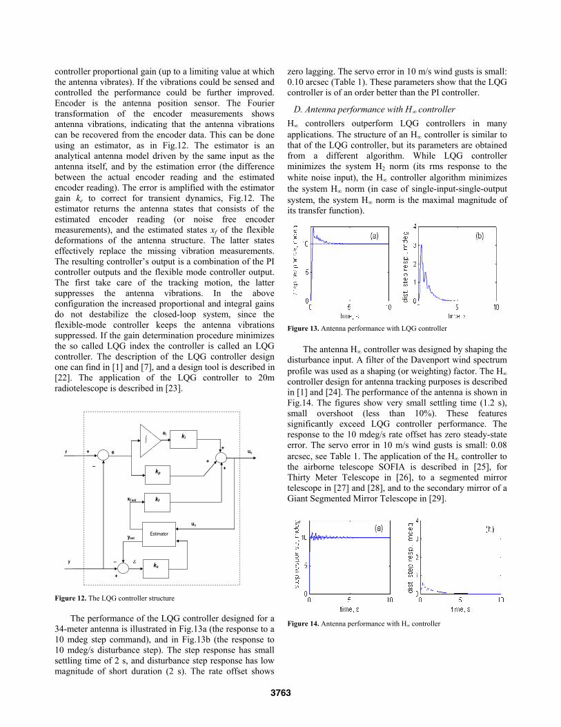
The antenna H controller was designed by shaping thedisturbance input. A filter of the Davenport wind spectrumprofile was used as a shaping (or weighting) factor. The Hcontroller design for antenna tracking purposes is describedin [1] and [24]. The performance of the antenna is shown inFig.14. The figures show very small settling time (1.2 s), small overshoot (less than 10%). These featuressignificantly exceed LQG controller performance. Theresponse to the 10 mdeg/s rate offset has zero steady-stateerror. The servo error in 10 m/s wind gusts is small: 0.08 arcsec, see Table 1. The application of the H controller tothe airborne telescope SOFIA is described in [25], forThirty Meter Telescope in [26], to a segmented mirrortelescope in [27] and [28], and to the secondary mirror of aGiant Segmented Mirror Telescope in [29].

uc

+

_

xf est

yest

+

ei

e

+

+

_

+ uc

y

r

ki

kp

kf

ke

Estimator

Figure 14. Antenna performance with H controller

3763

VII. COMMAND PREPROCESSORWhen LQG or H controller is implemented, it initiateslimit cycling during antenna slewing operations. Thisphenomenon is caused by the antenna rate and accelerationlimits: the controllers are designed for a linear plant, whilelimits cause antenna non-linear dynamics. In order to avoidthe cycling one can either apply different controllers fortracking purposes, and for slewing; or implement an anti-windup technique, see [30]; or apply a controller withvariable gains [20], [31]; or use a trajectory calculated inadvance, such that it never exceeds the rate and acceleration limits [32]; or use a command preprocessor(CPP). This paper presents the latter approach. The preprocessor is a computer program that generates a modified command, identical with the original one, if therate and accelerations are within the limits; and a commandof maximal (or minimal) rate and acceleration, when thelimits are met or violated. The location of the preprocessorin the antenna control system is shown in Fig.15.

Figure 15. The CPP location in the antenna control system

Figure 16. The CPP block diagram.

The block diagram of the CPP is shown in Fig.16. Itimitates a rigid antenna (represented by the integrator)driven by variable-gain controller with a feedforward gain(the latter represented by the derivative). The variable gainki depends on the preprocessor error ei as follows

iei o vk k k e (5)

In this equation ko is the constant part of the gain, kv is the variable part of the gain, and is the error exponential. The plot of ki(ei) for ko=1, kv=5, and =20 is shown in Fig.17.The detail description of CPP is given in [12].

The CPP response to the step of 10 deg is shown inFig.18. Preprocessed command begins with the maximalacceleration until it reaches the maximum rate, thencontinues with the maximal (and constant) rate and finallyslows-down with the minimal deceleration. After reaching

the value of 10 deg the error between the original and thepreprocessed command is zero.

Figure 17. The CPP gain versus CPP error.

The measured responses of the antenna to a large (non-processed) step input of 10 deg are shown in Fig.19a.Clearly, an unstable limit cycling is present. The sameresponse of the antenna with processed command is shownin Fig.19b, where the antenna follows closely the processedcommand, without limit-cycling.

Figure 18. The CPP response to 10-deg step

Figure 19. Antenna response to 10 deg step: (a) without CPP, and (b)with CPP.

10-4 10-3 10-2 10-1 1000

1

2

3

4

5

6

7

error, ei, deg

gain

,ki

y

rp u

CONTROLLER ANTENNA y CPP

r

acc. limitrate limit

0 2 4 6 8 10 12 14 16 18 200

2

4

6

8

10

time, s

AZ e

ncod

er, d

eg

+

+_+ rpiuiei vi

d/dt

ri ki

rate limitaccel. limit

0 5 10 15 20 25 30 35 400

2

4

6

8

10

12

time, s

DSS26 antenna response to 10 deg step

antenna without CPP

0 5 10 15 20 25 30 35 400

2

4

6

8

10

12

ante

nna

posi

tion,

deg

ante

nna

posi

tion,

deg

time, s

antenna withCPP

3764

VIII. POINTING ERROR SOURCESThe following is a list of the main pointing error sourcesthat are not detectable by the antenna sensors encoders):

The antenna encoders are not collocated with the RFbeam, thus the beam position is measured with a certain bias.The antenna control torques are applied at the motorlocations, while the wind disturbances are distributedover the antenna surface; thus only certain portion ofthe disturbances can be compensated with the motors..Disturbances. Thermal, and wind forces are the mainsources of disturbances and are difficult to measure.Gravity forces, and azimuth track imperfections aremeasurable and repeatable disturbances. Atmosphericrefraction is a measurable but unrepeatable disturbance.Model uncertainty. Manufacturing imperfections and the variable antenna configuration (its structuralproperties depend on its elevation angle) are the sourcesof uncertainty that limit the controller performance.Nonlinearities. Backlash and friction torques at theantenna drives, rate and acceleration limits are the mainsources of nonlinearity.

The pointing error sources and corrections for the GreenBank telescope are presented in [33]; for active correctionsof structural deformations see [34]; for trackingperformance [35]; on use of inclinometers for measuringtelescope position see [36]; on thermal and wind control ofthe Very Large Telescope (European SouthernObservatory) see [37].

A. Azimuth track imperfectionsAntenna rotates in azimuth on a circular azimuth track,which is manufactured with level precision of 0.5 mm forthe 34-m DSN antennas. The uneven azimuth track level causes antenna tilts and flexible deformations. The finiteelement model of the alidade (lower antenna structure)deformations due to track unevenness is shown in Fig.20.Certainly, these deformations impact antenna pointingaccuracy. However, the pointing errors caused by the trackirregularities are repeatable therefore they can becalibrated. By developing a look-up table one providespointing corrections as a function of the antenna azimuthposition. The look-up table is generated by usinginclinometers that measured tilts of the alidade structure atselected points.

Four inclinometers were installed on the alidadestructure, at locations marked in Fig.21. Each inclinometermeasures tilts of its x- and y-axes. The locations of theinclinometers were selected such that their tilts estimate thealidade elevation and cross-elevation rotations at theantenna focal point. Inclinometers No.1 and 2 are located atthe top of the alidade. Inclinometer No.2 is located next tothe elevation encoder. The y-axis tilt of this inclinometerreflects the elevation pointing error. Inclinometers No 3and 4 are located in the middle of the crossbeam of the leftand right sides of the alidade, respectively. Their x-axis tilts combined with the x-axis tilts of the inclinometers No.1

and 2, give the cross-elevation pointing error, as shownbelow.

Liftedwheel

Figure 20. Alidade deformation due to wheel lift.

Figure 21. Alidade and the inclinometer locations.

The x- and y-axis tilts of the ith inclinometer are denoted ix and iy, respectively. The inclinometer datawere collected during the antenna azimuth rotation atconstant rate of 50 mdeg/s, and the sampling frequency of2 Hz. The tests were performed during nighttime tominimize deformations of the antenna structure due to thethermal gradient. The data show satisfactory repeatability.

The antenna elevation error el is the y-tilt of the secondinclinometer

2el y (6)

3765

The cross-elevation error ( xel) depends on the antennaelevation position ( ), and on the rotation ( y) of the top ofthe alidade with respect to the y-axis (tilt of the elevationaxis) and the alidade twist z (the rotation of the top of thealidade with respect to the z-axis):

cos( ) sin( )xel z y (7)

The tilt of the elevation axis is an average of the x-tiltsof the inclinometers 1 and 2, that is,

1 20.5( )y x x (8)

while the alidade twist is determined from x-tilts of the inclinometer No3 and No4,

7 8( )z x x

hl

(9)

where h is the alidade height, and l is the distance betweenthe inclinometers. The details are in [38].

The reading of the inclinometer 1, x-axis, is shown in Fig.22. The fitted sinusoid shows the azimuth axis tilt. The pointing error obtained from the inclinometermeasurements is shown in Fig.23, dashed line. Themeasurements of the actual pointing error (using conscantechnique) are shown in the same figure, solid line with dots. The figure shows the coincidence of the inclinometerand conscan data.

0 50 100 150 200 250 300 350

-6

-4

-2

0

2

4

6

azimuth position, deg

incl

inom

eter

1,x

-tilt,

mde

g

Figure 22. Inclinometer No.1 tilt, x-direction.

100 110 120 130 140 150 160 170 180 190-8

-6

-4

-2

0

azimuth position, deg

EL

poin

ting

erro

r, m

deg

measured

from look-up table

Figure 23. Antenna elevation pointing error due to track level unevenness: from the look-up table (dashed line), and measured by conscan (solid line with dots)

B. Thermal deformations.The temperature gradient causes deformations of theantenna structure, thus it impacts the pointing accuracy.The inclinometers were used to measure antenna tilts when it was stowed. A sample shown in Fig.24 shows tilts of 8

mdeg. The largest tilts were in afternoons, when the sunheat was intensive (although the data were collected in November, which is not the hottest day at the MojaveDesert, where antennas are located). On techniques tocompensate for the thermal deformations see [39], [37],and [40].

C. Gravity deformationsGravity forces deform antenna dish and subreflector, andthe deformations depend on the dish elevation position.These deformations are repeatable and can be calculatedcomparatively accurately using the finite element model.The gravity deformations of the 70-meter antenna areshown in Fig.25. The calculated deformations allow togenerate a look-up table of the pointing corrections.

0 5 10 15 20 25 30 35 40 45-6

-5

-4

-3

-2

-1

0

1

2x 10 -3 inc linom eter1 , y -ax is

t im e, hours

tilt,

deg

day 1 day 2

Figure 24. Thermal deformations of the 34-meter DSN antenna.

Figure 25. Gravity deformation of the 70-meter antenna

D. Atmospheric refractionThe RF beam is bent while passing through the atmosphere, see Fig.26. The amount of refraction dependson air humidity, and can be calculated. The atmosphericconditions are monitored by weather stations, and refraction model calculates the correction once a second.The refraction corrections are added to the antenna pointing

3766

model, and they can be of order of several hundredmilidegrees.

E. FrictionA ope drive friction can cause pointing errors.

igure 26. Atmospheric refraction

F. BacklashG gears are an antenna drive components. A

IX. POINTING ERROR CORRECTION

A. LookT rrect for the known and repeatable

C feedback. This technique is

ntenna/telescIn order to improve pointing, the best thing is to reduce thefriction. For example the 70-meter DSN antennas use oilfilm to rotate in azimuth. Machine jack-screws, often usedin elevation drives, are sources of significant friction.When friction cannot be reduced through structuralmodifications a control engineering tools are implemented.One of them is dither, i.e., oscillations applied at thefriction source to break the friction contact. The ditherfrequency shall be higher than the antenna structuralfrequencies, to avoid excitation of structural resonances.The analysis of dither as applied to the antenna is given in [41]. The friction modeling of the 2.5 meter telescope is described in [42]; more on friction compensation, see [43],[44], and [45].

F

earboxes andbacklash phenomenon at the gearboxes is observed whenone gear rotates through a small angle without causing acorresponding movement of the second gear. This causesbeating in the drives, gear wear, and deterioration ofantenna tracking precision. In order to maintain antenna pointing precision the backlash phenomenon is eliminatedby implementing two symmetric drives with a specific torque difference between them, see Fig.27. The torque difference is called a torque bias, or counter-torque. Withtwo motor configurations the backlash clearance will occur at one drive while the other is still coupled. The antennadynamics will be controlled by the latter drive. Theeffectiveness of the two-motor approach depends on theamount of torque bias applied at the drives, which dependson the antenna variable load. The torque bias should belarge enough to lead the antenna through the gap for themaximal allowable torque load, but small enough that it will not cause excessive local stress, friction, or wear.

More on backlash, see [46], [47], [48], [49], [50], [51], [52]and [53].

-up tableshey are used to co

errors (e.g. gravity deformations, azimuth track levelcorrections). For non-repeatable errors an additionalfeedback (e.g., conscan or monopulse) is applied.

B. Conical scan (conscan)onscan is an additional

commonly used for the determination of the true spacecraftposition. During conscan, circular movements are added tothe antenna command as shown in Figure 28. The circularmovements cause sinusoidal variations of the power of thesignal received from the spacecraft, as illustrated in Fig.29. The power variations are used to estimate the truespacecraft position. The time of one cycle is between 30and 60 s, thus the correction update is comparatively slow.The drawback of this technique is that antenna is alwaysoff the peak power, i.e., always slightly off the target.

Figure 27. Motor torques and the counter-torque.

Figure 28. Antenna trajectory when performing conical scan.

80

-100 -80 -60 -40 -20 0 20 40 60 80 100-100

-80

-60

-40

-20

0

20

40

60

100

antenna load / max. antenna load, %

torque bias

motor 2

motor 1

motor 1+ motor2=antenna load

mot

orlo

ad /

max

. mot

orlo

ad,%

3767

The control system of the conscan consists of theadd

In the pointing error is estimated from RF

igure 29. Antenna power variation during conscan.

X. CONCLUSIONSThe paper presen t control systemengineers encounter while trying to satisfy the demandingpointing requirements. Not all challenges have satisfactory

scribed in this paper wascarried out by the Jet ory, California Institute of Tech ith the National

ics, and Active Controlof Structures, Springer, New York, 2004.

[2] W. Gawronski, and trol and Dynamics of the

itional (outer) feedback that corrects for the differencebetween encoder and RF beam position, see Fig.30. Moreabout conscan, see [54] and [55].

C. Monopulsethis algorithm

signals received by the monopulse feed-horn. These signals are uniquely related in amplitude and phase as a function ofthe antenna pointing error. The single monopulse feeddesign allows direct pointing at the target at all times,allowing for the spacecraft to be tracked at the peak of theantenna pattern. This technique is much faster than conscan(updating time is 0.02 s). More about monopulse see [56]and [57].

F

Figure 30. Antenna conscan controller.

ts the challenges tha

solutions. One of the reasons is the lack of a stable point ofreference to measure the RF beam position. The substitute beam position measurements using encoders are subject to painstaking corrections, which not always satisfy therequirements. A fast and inexpensive measurement systemof beam position would be a breakthrough in theantenna/telescope technology.

ACKNOWLEDGMENTA portion of the research de

Propulsion Laboratnology, under a contract w

Aeronautics and Space Administration.

REFERENCES[1] Gawronski, W., Advanced Structural Dynam

J.A. Mellstrom, "ConDeep Space Network Antennas," a chapter in Control and DynamicSystems, vol.63, ed. C.T. Leondes, Academic Press, San Diego,1994.

[3] W. Gawronski and K. Souccar, “Control system of the LargeMillimeter Telescope,” SPIE Astronomical Telescopes andInstrumentation Conference, Glasgow, June 2004.D. Cla[4] rk “Control system prototyping – A case study” TechnicalMemo, ITM-04-3,www.mmto.org/MMTpapers/tech00_10.shtml#2004T. Erm and P. Gutierrez, “Integration and tuning o[5] f the VLT drivesystems,” Proc. SPIE Telescope Structures, Enclosures, Controls,Assembly/Integration/Validation and Commissioning, Vol.4004,2000.

[6] S. Jimenez-Garcia, M.E. Magana, J.S. Benitez-Read, and J.Martinez-Carbalido, “Modeling, simulation, and gain schedulingcontrol of large radiotelescopes,” Simulation Practice and Theory,vol. 8, pp.141-160, 2000.

[7] W. Gawronski, C. Racho, and J. Mellstrom, "Application of theLQG and feedforward controllers for the DSN antennas," IEEETrans. on Control Systems Technology, vol.3, 1995, also see tmo.jpl.nasa.gov/tmo/progress_report/42-109/109R.PDF,tmo.jpl.nasa.gov/tmo/progress_report/42-112/112J.PDF.W. Gawronski, H. G. Ahlstrom, and A. M. Bernardo, “Analysis and performance of the control systems of the NASA 70

[8]meter-

antennas,” ISA Transactions, 2004, also see tmo.jpl.nasa.gov/tmo/progress_report/42-144/144D.pdf

[9] D. Clark, “Selected results of recent MMT servo testing,”Technical Memo, ITM-03-5,

5.pdfwww.mmto.org/MMTpapers/pdfs/itm/itm03-[1 ] E. Cascone, D. Mancini, and P. Schipani, “Galileo Telesc0 ope model

identification,” Proc. SPIE, vol. 3112, pp.343-350, 1997.E. Simiu and R.H. Scanlan,[11] Wind Effects on StructNew York 1978.

ures, Wiley,

[12] W. Gawronski, W. Almassy, “Command pre-processor forradiotelescopes and microwave antennas,” IEEE Antennas andPropagation Magazine, vol.44, No2, 2002, also seehtmo.jpl.nasa.gov/tmo/progress_report/42-136/136A.pdf ipnpr.jpl.nasa.gov/tmo/progress_report/42-150/150G.pdfW. Gawronski, B. Bienkiewicz, and R.E. Hill, "Wind-induceddynamics of a Deep Space Network antenna," Journa

[13]ndl of Sound a

Vibration, vol.178, No.1, 1994, also see tmo.jpl.nasa.gov/tmo/progress_report/42-108/108J.PDF

[14] W. Gawronski, “Modeling Wind Gusts Disturbances for theAnalysis of Antenna Pointing Accuracy,” IEEE Antennas andPropagation Magazine, vol.46, 2004, also seeipnpr.jpl.nasa.gov/tmo/progress_report/42-149/149A.pdf

[15] G.Z. Angeli, M.K. Cho, M. Sheehan, and L.M. Stepp,“Characterization of Wind Loading of Telescopes,” Proc. SPIE,Integrated Modelingvof Telescopes,vol. 4757, pp.72-83, 2002.

antennacontroller antenna

encoder

conscanestimator

conscancontroller

beamposition

command

3768

[16] W. Gawronski, J. Mellstrom and B. Bienkiewicz, “Antenna Mean Wind Torques: A Comparison of Field and Wind Tunnel Data,” IEEE Antennas and Propagation Magazine, 2004.

[17] J. Mann, “Wind field simulations, Prob. Engrg. Mech., vol. 13, pp. 269-282, 1998. W. Gawronski, "Predictive controller and estima[18] tor for NASA

s, Measurements, and Control, No2, 1994, also see Deep Space Network antennas," ASME Transactions, Journal of Dynamic Systemtmo.jpl.nasa.gov/tmo/progress_report/42-104/104D.PDF.T. Erm, and S. Sandrock, “Adaptive periodic error correction for the VLT telescopes,” Proc. SPIE Large Ground-Based Telescopes,

[19]

[22] ronski, “LQG controller design using GUI:

40D.pdf

Vol. 4837-106, 2002 [20] D. Mancini, M. Brescia, E. Cascote, P. Schipani, “A variable

structure control law for telescopes pointing and tracking,” Proc. SPIE, vol.3086, 1997.

[21] W. Gawronski, “Antenna control systems: from PI to H ,” IEEE Antennas and Propagation Magazine, vol.43, no.1, 2001 Maneri, E., and W. Gawapplication to antennas and radio-telescopes,” ISA Transactions, 2000, also tmo.jpl.nasa.gov/tmo/progress_report/42-140/1

sa.gov/tmo/progress_report/42-

[23] M. Olberg, C. Lindeborg, A. Seyf, and C.F. Kastengren, “A simple robust digital controller for the Onsala 20m radio telescope,” Proc. SPIE, vol. 2479, pp.257-265, 1995.

[24] Gawronski, W. "H controller for the DSS13 antenna with wind disturbance rejection properties,” TDA Progress Report, vol.42-127, November 1996, tmo.jpl.na127/127G.pdf U. Schoenhoff, A. Klein, and R. Nordmann, “Attitude control of the airborne telescope SOFIA: -synthesis for a large scaled flexible structure,” th

[25]

Proc. 39 IEEE Conf. Decision and Control,

[26]

5496, 2004.

Systems Magazine,

[28]

Conference on Decision and Control, Tampa, FL,

[29]

pes, vol.4840, 2003.

.4, 1996.

97.

/118E.pdf

Sydney, Australia, 2000. T. Erm, B.Bauvir, and Z. Hurak, “Time to go H-infinity?” Proc. SPIE, Advanced Software, Control, and Communication Systems for Astronomy, Glasgow, UK, vol.

[27] K. Li, E.B. Kosmatopoulos, P.A. Ioannou, and H. Ryaciotaki-Boussalis, “Large segmented telescopes: Centralized, decentralized and overlapping control designs,” IEEE Control October 2000. K. Li, E.B. Kosmatopoulos, P.A. Ioannou, H. Boussalis, and A. Chassiakos, “Control techniques for a large segmented reflector,” Proc. 37th IEEE1998. M. Whorton, G. Angeli, “Modern control for the secondary mirror of a Giant Segmented Mirror Telescope,” Proc. SPIE, Future Giant Telesco

[30] Y. Peng, D. Vrancic, and R. Hanus, “Anti-windup, bumpless, and conditioned transfer techniques for PID controllers,” IEEE Control Systems Magazine, vol.16, No

[31] D. Mancini, M. Brescia, E. Cascote, P. Schipani, “A neural variable structure controller for telescopes pointing and tracking improvement,” Proc. SPIE, vol.3112, 19

[32] Tyler, S. R., "A trajectory preprocessor for antenna pointing," TDA Progress Report, 42-118, pp. 139-159, 1994, tmo.jpl.nasa.gov/tmo/progress_report/42-118

Control Software,

ontrols, Assembly/Integration/Validation and

[35]

[36] ace, and D. Cowley “Tests of a

alidation and Commissioning,vol. 4004,

[38]compensation to reduce blind pointing errors of the Deep Space

lso tmo.jpl.nasa.gov/tmo/progress_report/42-139/139D.pdf

[33] J.J. Brandt, “Controlling the Green Bank Telescope,” Proc. SPIE, “Advanced Telescope and Instrumentationvol.4009, 2000.

[34] H. Baier, and G. Locatelli, “Active and passive microvibration control in telescope structures,” Proc. SPIE, Telescope Structures, Enclosures, CCommissioning, vol. 4004, 2000. T.Erm, “Analysis of tracking performance,” Proc. SPIE, Optical Telescopes Of Today And Tomorrow, vol.2871, p 1032-1040, 1996 R. Kibrick, L. Robinson, V. Wallprecision tiltmeter system for measuring telescope position,” Proc. SPIE, vol.3351, 1998.

[37] M. Cullum, and J. Spyromilio, “Thermal and wind control of the VLT,” Proc. SPIE, Telescope Structures, Enclosures, Controls, Assembly/Integration/V2000. W. Gawronski, F. Baher, and O. Quintero: “Azimuth track level

Network antennas,” IEEE Antennas and Propagation Magazine,2000, a .

[40]

[41] telesope low rate tracking

[42] , and S. Hansen, “Friction model of the 2.5 mts SDSS

[43]ed Kalman-Bucy filter friction estimation: a

[45] emster, P. Vedagarbha, D.M. Dawson, and D. Haste,

[46] .O. Gutman, “Controlling mechanical systems

[47] nd compensation

[48] ata-Jimenez, B. Brogliato, and A. Goswami “On the control

[49] s with parasitic effects,”

[50]s, Measurement, and

[51] tection in

[52] rlin, J.G. Ingalis, J. Cheng, and G. Wright,

2000, also see tmo.jpl.nasa.gov/tmo/progress_report/42-

[39] A. Greve, M. Dan, and J. Penalver, “Thermal behavior of millimeter wavelength radio telescopes,” IEEE Trans. on Antennas and Propagation, vol.40, No.11, 1992. A. Greve, G. MacLeod, “Thermal model calculations of enclosures for millimeter wavelength radio telescopes,” Radio Science, Vol.36, No.5, 2001. Gawronski, W., and Parvin, B., "Radiousing dither,” AIAA Journal of Guidance, Control, and Dynamics,vol.21, 1998. C. H. Rivettatelescope,” Proc. SPIE, vol.3351, 1998.A. Ramasubramanian, L.R. Ray, “Adaptive friction compensation using extendcomparative study,” Proc. American Control Conf., Chicago, IL, 2000.

[44] J. Moreno, R. Kelly, and R. Campa, “On velocity control using friction compensation,” Proc 41st Conf. Decision and Control, Las Vegas, NV, 2002. M. Fe“Adaptive control techniques for friction compensation,” Proc. American Control Conf., Philadelphia, PA, 1998. M. Nordin, and Pwith backlash—a survey,” Automatica, vol.38, pp.1633-1649, 2002. R. Dhaouadi, K. Kubo, and M. Tobise, “Analysis aof speed drive system with torsional loads,” IEEE Trans. on Industry Applications, vol.30, No.3, 1994. M.T. Mof mechanical systems with dynamics backlash,” Proc 36th Conf. Decision and Control, San Diego, CA, 1997. B. Friedland, “Feedback control of systemProc. American Control Conf., Albuquerque, NM, 1997. J.L. Stein, and C.-H. Wang, “Estimation of gear backlash: Theory and simulation,” Journal of Dynamic SystemControl, vol. 120, 1998. N. Sarkar, R.E. Ellis, and T.N. Moore, “Backlash degeared mechanisms: Modeling, simulation, and experimentation,” Mechanical Systems and Signal Processing, vol.11, No.3, 1997. A.A. Stark, R.A. Chambe“Optical and mechanical design of the Antarctic Submillimeter Telescope and Remote Observatory,” Rev. Sci. Instrumm vol.68, 1997.

[53] W. Gawronski, J.J. Brandt, H.G. Ahlstrom, Jr., and E. Maneri: “Torque bias profile for improved tracking of the Deep Space Network antennas,” IEEE Antennas and Propagation Magazine,Dec. 139/139F.pdfW. Gawronski, and E. Craparo “Antenna scanning techniques for estimation of spacecraft position,” IEEE Antennas and Propagation Magazine, vol.44, no.6, Dec. 2002, also see

[54]

ov/tmo/progress_report/42-147/147B.pdfipnpr.jpl.nasa.g

[56] nd D. M.

1-29, August 15, 1999,

[55] N. Levanon, “Upgrading conical scan with off-boresight measurements,” IEEE Trans. Aerospace and Electronic Systems,vol.33, No.4, 1997. Gudim, M. A., W. Gawronski, W. J. Hurd, P. R. Brown, aStrain, "Design and performance of the monopulse pointing system of the DSN 34-meter beam-waveguide antennas," TMO PR 42-138, April-June 1999, pp.tmo.jpl.nasa.gov/tmo/progress_report/42-138/138H.pdf Gawronski, W., and M.A. Gudim, “Design and performance of the monopulse control system," IEEE Antennas and Propagation Magazine, 1999, also see

[57]

o/progress_report/42-tmo.jpl.nasa.gov/tm137/137A.pdf .

3769