Helsinki University of Technology Signal Processing LaboratoryTeknillinen korkeakoulu Signaalinkasittelytekniikan laboratorioEspoo 2004 Report 47

CONTRIBUTIONS TO THEORY AND ALGORITHMS OFINDEPENDENT COMPONENT ANALYSIS AND SIGNALSEPARATION

Jan Eriksson

Dissertation for the degree of Doctor of Science in Technology to be pre-sented with due permission of the Department of Electrical and Communi-cations Engineering for public examination and debate in Auditorium S4 atHelsinki University of Technology (Espoo, Finland) on the 20th of August,2004, at 12 noon.

Helsinki University of TechnologyDepartment of Electrical and Communications EngineeringSignal Processing Laboratory

Teknillinen korkeakouluSahko- ja tietoliikennetekniikan osastoSignaalinkasittelytekniikan laboratorio

Distribution:Helsinki University of TechnologySignal Processing LaboratoryP.O. Box 3000FIN-02015 HUTTel. +358-9-451 3211Fax. +358-9-452 3614E-mail: Mirja.Lemetyinen@hut.fi

c© Jan Eriksson

ISBN 951-22-7224-5 (Printed)ISBN 951-22-7227-X (Electronic)ISSN 1458-6401

Otamedia OyEspoo 2004

Abstract

This thesis addresses the problem of blind signal separation (BSS) usingindependent component analysis (ICA). In blind signal separation, signalsfrom multiple sources arrive simultaneously at a sensor array, so that eachsensor array output contains a mixture of source signals. Sets of sensoroutputs are processed to recover the source signals or to identify the mix-ing system. The term blind refers to the fact that no explicit knowledge ofsource signals or mixing system is available. Independent component anal-ysis approach uses statistical independence of the source signals to solvethe blind signal separation problems. Application domains for the materialpresented in this thesis include communications, biomedical, audio, image,and sensor array signal processing.

In this thesis reliable algorithms for ICA-based blind source separationare developed. In blind source separation problem the goal is to recover alloriginal source signals using the observed mixtures only. The objective is todevelop algorithms that are either adaptive to unknown source distributionsor do not need to utilize the source distribution information at all. Twoparametric methods that can adapt to a wide class of source distributionsincluding skewed distributions are proposed. Another nonparametric tech-nique with desirable large sample properties is also proposed. It is basedon characteristic functions and thereby avoids the need to model the sourcedistributions. Experimental results showing reliable performance are givenon all of the presented methods.

In this thesis theoretical conditions under which instantaneous ICA-based blind signal processing problems can be solved are established. Theseresults extend the celebrated results by Comon of the traditional linear real-valued model. The results are further extended to complex-valued signalsand to nonlinear mixing systems. Conditions for identification, uniqueness,and separation are established both for real and complex-valued linear mod-els, and for a proposed class of non-linear mixing systems.

iii

Preface

The work constituting this thesis was carried out in the Signal ProcessingLaboratory at Helsinki University of Technology during years 2000–2004.The research group is a member of SMARAD, Center of Excellence of theAcademy of Finland.

I wish to express my deep gratitude to my supervisor Prof. VisaKoivunen for his continuous encouragement, guidance and support duringthe course of this work. I especially admire his excellent work ethic anddedication to the science. It has been a real pleasure to work with him.

I would like to thank the thesis pre-examiners, Prof. Christian Juttenand Dr. Arie Yeredor, for their constructive and helpful comments thatimproved the manuscript a lot. Prof. Iiro Hartimo, the director of Grad-uate School in Electronics, Telecommunications and Automation (GETA)and the GETA coordinator Marja Leppaharju are also highly acknowledged.Many thanks go to our laboratory secretaries Mirja Lemetyinen and AnneJaaskelainen for the help with all the practical issues and arrangements.

I am grateful to all the colleagues in the lab and especially co-workers Dr.Annaliisa Kankainen and Dr. Juha Karvanen. Prof. Risto Wichman, Dr.Samuli Visuri, Dr. Mihai Enescu, Dr. Marius Sirbu, Dr. Esa Ollila, MaaritMelvasalo, Timo Roman and Traian Abrudan are also acknowledged for ourmany interesting discussions, not only research related. I would like to givemy warmest thanks to my parents, Terttu and Trygve, and to my sister,Tiia, for all their support. I am also thankful to all my friends, in particularJarkko and Ville, for the quality leisure time and memorable moments.

The financial support from Academy of Finland, GETA, Nokia Founda-tion and Jenny and Antti Wihuri Foundation is gratefully acknowledged.

Finally, the work put into this thesis was worthwhile due to Sanna, theforemost source of happiness in my life. Thank you so much.

Espoo, August 2004

Jan Eriksson

iv

Contents

Abstract iii

Preface iii

List of original publications vi

List of abbreviations and symbols ixAbbreviations . . . . . . . . . . . . . . . . . . . . . . . . . . . ixSymbols . . . . . . . . . . . . . . . . . . . . . . . . . . . . . . ix

1 Introduction 11.1 Motivation . . . . . . . . . . . . . . . . . . . . . . . . . . . . 11.2 Scope of the thesis . . . . . . . . . . . . . . . . . . . . . . . . 31.3 Contribution of the thesis . . . . . . . . . . . . . . . . . . . . 31.4 Summary of publications . . . . . . . . . . . . . . . . . . . . . 4

2 Overview of ICA 72.1 Problem formulation and general assumptions . . . . . . . . . 72.2 Anatomy of ICA methods . . . . . . . . . . . . . . . . . . . . 82.3 Measuring stochastic independence . . . . . . . . . . . . . . . 9

2.3.1 Correlation . . . . . . . . . . . . . . . . . . . . . . . . 92.3.2 Mutual Information . . . . . . . . . . . . . . . . . . . 102.3.3 Characteristic function, generating functions, mo-

ments and cumulants . . . . . . . . . . . . . . . . . . . 112.3.4 Complex random variables . . . . . . . . . . . . . . . 122.3.5 Discussion . . . . . . . . . . . . . . . . . . . . . . . . . 14

2.4 Review of optimization algorithms . . . . . . . . . . . . . . . 142.4.1 Gradient descent methods . . . . . . . . . . . . . . . . 152.4.2 Jacobi algorithms . . . . . . . . . . . . . . . . . . . . . 16

2.5 Discussion . . . . . . . . . . . . . . . . . . . . . . . . . . . . . 17

3 Identifiability, separability, and uniqueness of linear ICAmodels 193.1 Real-valued linear instantaneous ICA model . . . . . . . . . . 19

v

3.1.1 Identifiability . . . . . . . . . . . . . . . . . . . . . . . 213.1.2 Separability . . . . . . . . . . . . . . . . . . . . . . . . 223.1.3 Uniqueness . . . . . . . . . . . . . . . . . . . . . . . . 223.1.4 Discussion . . . . . . . . . . . . . . . . . . . . . . . . . 25

3.2 Complex linear instantaneous signal model . . . . . . . . . . 253.2.1 Identifiability, separability, and uniqueness . . . . . . . 26

3.3 Discussion . . . . . . . . . . . . . . . . . . . . . . . . . . . . . 27

4 Nonlinear instantaneous ICA models 284.1 Models implied by Addition Theorem . . . . . . . . . . . . . 284.2 Post-nonlinear model . . . . . . . . . . . . . . . . . . . . . . . 314.3 Discussion . . . . . . . . . . . . . . . . . . . . . . . . . . . . . 32

5 Source adaptive methods for blind separation 345.1 Overview of mutual information-based separation methods . . 345.2 Extended generalized lambda distribution . . . . . . . . . . . 365.3 Pearson system . . . . . . . . . . . . . . . . . . . . . . . . . . 385.4 Discussion . . . . . . . . . . . . . . . . . . . . . . . . . . . . . 39

6 Characteristic function-based methods for blind separation 416.1 Cumulant-based methods . . . . . . . . . . . . . . . . . . . . 416.2 Characteristic function enabled source separation . . . . . . . 426.3 Jacobi optimized empirical characteristic function ICA . . . . 436.4 Discussion . . . . . . . . . . . . . . . . . . . . . . . . . . . . . 44

7 Conclusion 477.1 Summary . . . . . . . . . . . . . . . . . . . . . . . . . . . . . 477.2 Future work . . . . . . . . . . . . . . . . . . . . . . . . . . . . 48

Bibliography 50

Publications 59Errata . . . . . . . . . . . . . . . . . . . . . . . . . . . . . . . 59

vi

List of original publications

(I) J. Eriksson, J. Karvanen, and V. Koivunen. Source distribution adap-tive maximum likelihood estimation of ICA model. In Proc. of Sec-ond International Workshop on Independent Component Analysis andBlind Source Separation (ICA 2000), pp. 227–232, Helsinki, Finland,June 2000.

(II) J. Karvanen, J. Eriksson, and V. Koivunen. Pearson system basedmethod for blind separation. In Proc. of Second International Work-shop on Independent Component Analysis and Blind Source Separa-tion (ICA 2000), pp. 585–590, Helsinki, Finland, June 2000.

(III) J. Karvanen, J. Eriksson, and V. Koivunen. Adaptive Score Functionsfor Maximum Likelihood ICA. Journal of VLSI Signal Processing, 32:83–92, 2002.

(IV) J. Eriksson and V. Koivunen. Blind separation using characteristicfunction based criterion. In Proc. of 35th Conference on InformationSciences and Systems (CISS 2001), vol. 2, pp. 781–785, Baltimore,Maryland, March 2001.

(V) J. Eriksson, A. Kankainen, and V. Koivunen. Novel characteristicfunction based criteria for ICA. In Proc. of Third International Con-ference on Independent Component Analysis and Blind Source Sep-aration (ICA 2001), pp. 108–113, San Diego, California, December2001.

(VI) J. Eriksson and V. Koivunen. Blind identifiability of class of nonlin-ear instantaneous ICA models. In Proc. of the XI European SignalProcessing Conference (EUSIPCO 2002), vol. 2, pp. 7–10, Toulouse,France, September 2002.

(VII) J. Eriksson and V. Koivunen. Characteristic-function-based indepen-dent component analysis. Signal Processing, 83: 2195-2208, 2003.

(VIII) J. Eriksson and V. Koivunen. Identifiability, separability, and unique-ness of linear ICA models. IEEE Signal Processing Letters, vol. 11,No. 7, pp. 601–604, July 2004.

vii

(IX) J. Eriksson and V. Koivunen. Complex Random Vectors and ICAModels: Identifiability, Uniqueness and Separability. Submitted toIEEE Transactions on Information Theory, March 2004. Materialpresented also in the technical report: Identifiability, Separability, andUniqueness of Complex ICA Models. Signal Processing LaboratoryTechnical Report 44, Helsinki University of Technology, 2004, ISBN951-22-6774-8, ISSN 1458-6401.

viii

Abbreviations and symbols

Abbreviations

BSP blind signal processingBSS blind source/signal separationc.f. characteristic functionCHESS characteristic function enabled source separationd.f. distribution functione.c.f. empirical characteristic functionEGLD extended generalized lambda distributionGBD generalized beta distributionGLD generalized lambda distributioni.i.d. independent identically distributedICA independent component analysisJECFICA Jacobi optimized empirical characteristic function ICAm.g.f. moment generating functionm.i. mutual informationMIMO multiple-input multiple-outputp.d.f. probability density functionPCA principal component analysisPNL post-nonlinearr.v. random variabler.vc. random vectors.c.f. second characteristic function

Symbols

A, B mixing matrixα column of a matrix, real vectora, b scalar constantC field of complex numbersE(·)

{·}

expectation operatorFx distribution function of a random variable x

ix

fx probability density function of a random variable xF{·} system operatorF(·), G(·), H(·) vector-valued functionF(·), G(·), H(·) scalar-valued functionH(x) entropy of a random vector x

AH hermitian transpose of a matrix AI identity matrix imaginary unit, 2 = 1k, l, n discrete indexKL

(fx, fs

)Kullback-Leibler divergence betweenprobability density functions fx and fs

MI(x) mutual information of a random vector xm number of sourcesn[·] discrete-time noise signalN set of natural numbers 0, 1, 2, . . .p number of mixturesP permutation matrixP(·) polynomialR field of real numberss[·] discrete-time source signals, r random vector (sources)s, r random variable (source)AT transpose of a matrix At, x real vectort, x, y, u, v real variableU , V orthonormal matrixW separating matrixx[·] discrete-time mixture signalx, y random vectorx, y random variablez complex vectorΛ diagonal matrixφx characteristic function of a random variable xφx empirical characteristic function of a random variable xψx second characteristic function of a random variable xϕx score function of a random variable xϕx vector of score functions of the marginals of a random vector x∇F gradient of a function F∇NF natural gradient of a function F

x

Chapter 1

Introduction

1.1 Motivation

Multichannel observations are often encountered in signal processing appli-cation areas. For example, there may be several microphones recording thesound waves in audio and speech signal processing, in biomedical signal pro-cessing there are several sensors measuring e.g. heart or brain activity, andin communication systems multiple antennas are receiving the communica-tion signals. Multiple time series may be describing the same phenomenon,e.g. consumer confidence, in econometrics, and several images, e.g. in dif-ferent wave lengths or from different angles, may be available from the sameobject in image processing. These measurements can be obtained over aperiod of time (e.g. in communications), or over a certain surface area (e.g.in image processing). Such measurements can be then discretized such thatthere is a collection of observation vectors, each vector representing all mea-surements from different sensors at a specific observation time instant orspatial location.

Often each of these several measurements is a mixture of some sourcesignals. For instance, each communication antenna receives the superposi-tion of all communication signals transmitted in the same carrier frequency,and each sensor measuring the brain activity records the brain activity sig-nals coming from different areas of the brain. Although different sensorsmay be recording a mixture of the same source signals, the measurementsmay be different in all sensors due to the differences in e.g. positions of thesensors. For instance, each antenna receives each transmitted signal from adifferent angle with different amplitude depending the relative positioningof the transmitter and the antenna. Systems with multiple signal emittersand multiple sensors used for observing them are generally called multiple-input multiple-output (MIMO) systems. An example of a MIMO system isillustrated in Figure 1.1.

In blind source separation (BSS) the observations from a MIMO system

1

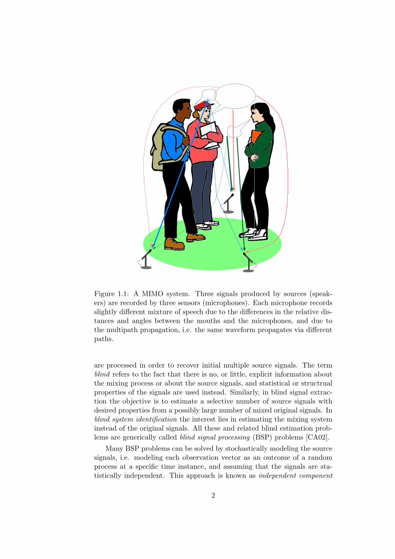
Figure 1.1: A MIMO system. Three signals produced by sources (speak-ers) are recorded by three sensors (microphones). Each microphone recordsslightly different mixture of speech due to the differences in the relative dis-tances and angles between the mouths and the microphones, and due tothe multipath propagation, i.e. the same waveform propagates via differentpaths.

are processed in order to recover initial multiple source signals. The termblind refers to the fact that there is no, or little, explicit information aboutthe mixing process or about the source signals, and statistical or structrualproperties of the signals are used instead. Similarly, in blind signal extrac-tion the objective is to estimate a selective number of source signals withdesired properties from a possibly large number of mixed original signals. Inblind system identification the interest lies in estimating the mixing systeminstead of the original signals. All these and related blind estimation prob-lems are generically called blind signal processing (BSP) problems [CA02].

Many BSP problems can be solved by stochastically modeling the sourcesignals, i.e. modeling each observation vector as an outcome of a randomprocess at a specific time instance, and assuming that the signals are sta-tistically independent. This approach is known as independent component

2

analysis (ICA). Recent textbooks [CA02, HKO01, Hay00] provide a goodintroduction to ICA-based BSP.

1.2 Scope of the thesis

The purpose of this thesis is to further develop the theory of ICA-basedblind signal processing, and derive algorithms for practical ICA-based blindsource separation. This thesis considers only the situation where there is notime dependency in the mixing system, i.e. the system is instantaneous, norany time dependency in the source signals themselves, i.e. each source signalis considered as an outcome of a random process that consist of independentidentically distributed (i.i.d.) random variables. Some results on ICA-basedmethods utilizing time structure in the system, e.g. convolutive mixing, orin the source signals, e.g. autocovariance, can be found from [CA02, HKO01,Hay00].

The first goal of this thesis is to develop reliable algorithms for ICA-based blind source separation. The objective is to develop algorithms thatare either adaptive to unknown source distributions or do not need to utilizethe source distribution information at all. The algorithms should performreliably for all type of source signals, and their performance should improveas there are more observations available (consistency).

The second goal of this thesis is to establish theoretical conditions underwhich instantaneous ICA-based BSP problems can be solved. This includesthe traditional linear real-valued model and its extensions to complex-valuedsignals and to nonlinear mixing systems. The conditions should be estab-lished for identification, extraction, and separation type of BSP problems.

1.3 Contribution of the thesis

The contributions of this thesis include the following.

• Extended Generalized Lambda Distribution (EGLD) is proposed asan adaptive score function model in the ICA separation problem.

• The use of L-moments is proposed for the estimation of the GeneralizedLambda Distribution (GLD) and the use of Pearson system in the ICAseparation problem is introduced in co-operation with the co-authors.

• Characteristic function-based method is proposed for the ICA separa-tion problem. The connection of the criterion to nonlinear correlations-based independence characterization is derived.

• Consistent characteristic function-based objective function is proposedfor the ICA separation problem. Consistency being established in

3

[CB04]. Novel minimization algorithm for the consistent objectivefunction is developed, and connection to the cumulant-based methodsis established.

• The concept “uniqueness” is introduced to the ICA models. Separa-bility conditions for the real-valued linear ICA model are extended tonecessary conditions by removing earlier requirement of finite second-order moments. Conditions for identifiability and uniqueness are es-tablished.

• A class of nonlinear ICA models is introduced, and the separabilityof the class is established. A generic algorithm for separation of thesemodels is proposed. A nonlinear ICA model is applied to an imageenhancement problem.

• Conditions for separability, identifiability, and uniqueness of complex-valued ICA models are established. The condition for separability isshown to be sufficient and necessary.

• A characterization of second-order structure of circular and non-circular complex-valued random vectors, a decomposition of complexnormal random vector, and extensions of the Darmois-Skitovich theo-rem to complex-valued random variables are established.

1.4 Summary of publications

This thesis consists of nine publications and a summary. The summary partof the thesis is organized as follows: Chapter 2 introduces the general ICAmodel and reviews the related probabilistic concepts and optimization algo-rithms. The theoretical conditions for linear real and complex-valued ICAmodels are summarized in Chapter 3. Chapter 4 introduces a class of non-linear ICA models and reviews are related nonlinear model. Source adaptiveICA separation methods are reviewed and Pearson and EGLD-based meth-ods are summarized in Chapter 5. Chapter 6 reviews characteristic function-based ICA methods and summarizes the JECFICA algorithm. Chapter 7provides a brief summary and outlines future research.

In Publication I, a EGLD-based BSS method is introduced. An ICAmethod utilizing the method of moments for fitting the EGLD, the mutualinformation contrast, and the fixed point algorithm [H+] is proposed. Thegood performance of the algorithm is demonstrated in simulations.

In Publication II, a Pearson system-based BSS method is introduced. AnICA method utilizing the method of moments for finding the parameters ofthe Pearson system, the mutual information contrast, and the fixed pointalgorithm [H+] is proposed. The simulation examples demonstrate that themethod can separate both super- and sub-Gaussian sources.

4

In Publication III the methods proposed in Publication I and in Publica-tion II are further studied and compared. It is demonstrated in simulationsthat the standard BSS methods may perform poorly in the cases wherethe sources have asymmetric distributions. Due to source adaptation theEGLD and Pearson system based methods reliably separate the sources.Additionally the method of L-moments is proposed for the estimation ofGLD parameters.

Publication IV proposes the use of characteristic functions to solve reli-ably the ICA-based BSS problem without need to model the source distri-butions. The method utilizing empirical characteristic functions, pairwiseprocessing, and golden section search is proposed. The reliable performanceis demonstrated in simulations.

Publication V improves the method of Publication IV by introducing theconsistent objective functions. The consistency of such objective functionswas recently shown in [CB04]. Additionally, a connection between the twodimensional criterion introduced in Publication IV and the independencecharacterization by nonlinear correlations is established.

Publication VI introduces a class of nonlinear ICA models. The condi-tions for separability are established, and a generic method for separation isproposed. An application to image enhancement is presented.

In Publication VII the characteristic function-based methods of Publica-tion IV and of Publication V are further developed. A fast minimization ofthe two dimensional objective function based on Fourier series representationis proposed. A connection to cumulant-based methods is established, andcriteria for noisy ICA are proposed. Further extensive simulations highlightthe highly reliable performance of the proposed method.

The sufficient conditions for separability, identifiability, and uniquenessof real-valued linear ICA models are established in Publication VIII. Theconditions for separability are proved to be necessary thereby extending theseminal results by Comon [Com94].

The sufficient conditions for separability, identifiability, and uniquenessof complex-valued linear ICA models are established in Publication IX. Theconditions for separability are also found to be necessary. A novel charac-terization of the second-order structure of complex random vectors, and adecomposition of complex normal random vectors is derived. This is ap-plied to derive the characteristic functions and the entropy of complex nor-mal random vector. Also extensions of the Darmois-Skitovich theorem tocomplex-valued random variables are presented.

The author of this thesis proposed the use of EGLD system and derivedthe analytical results in Publication I. The experiments were performed andthe writing was done in co-operation with co-authors.

In Publication II, the idea of using the Pearson system for the score func-tion modeling is due to Juha Karvanen. Also the idea of using L-momentsfor estimating the EGLD parameters, proposed in Publication III, is due to

5

him. The implementation of the ICA method, the experiment designs, andwriting were done by Jan Eriksson in co-operation with the co-authors.

The results in publications IV–IX were derived independently by the au-thor of this thesis. Visa Koivunen contributed in steering the research, andhelped in writing and structuring the publications. Annaliisa Kankainen,the second author of Publication V, helped providing useful references.

6

Chapter 2

Overview of ICA

2.1 Problem formulation and general assumptions

The general discrete-time blind source separation (BSS) system model isdescribed by the input-output relationship

x[k] = F{s[k], n[k]}, (2.1)

where k is the discrete time index, x[k] is the observed multidimensionalmixture signal and n[·] is the noise. The goal of BSS is to reconstruct theoriginal source signal s[k] and/or identify the system operator F{·} fromthe observed mixture signal without explicit knowledge of the source signalsnor the system operator. The term blind is used to distinguish the problemfrom the cases, where there is some explicit information available, e.g. aknown training source signal.

The general problem of Eq. (2.1) is naturally ill-posed, and further con-straints are needed. A common approach is to model the signals stochasti-cally, that is, to view the source signal as a realization of a random process.Then one can exploit statistical properties of the processes e.g. in time or inspace to obtain the goal. A relatively recent approach is to try to obtain thesolution based on the assumption that the source signals are stochasticallymutually independent. This approach is known as independent componentanalysis (ICA). If the system is memoryless, the model is called instanta-neous ICA, and the problems where noise is taken into account the modelis known as noisy ICA. If the signals have no time structure, then they aretypically assumed to be vector random processes of independent identicallydistributed (i.i.d.) random vectors (r.vc.’s). Thus the general instantaneoustime-independent noiseless ICA model is described by the equation

x = F(s), (2.2)

where (s1, . . . , sm)T = s are unknown mutually independent non-degeneraterandom variables (r.v.’s) called sources, F(·) is an unknown mixing function,

7

and x = (x1, . . . , xp)T are mixtures, i.e., the observed r.vc. (sensor arrayoutput). In the traditional setting, the mixing functions are constrained tobe matrices, i.e. linear mappings, and the ICA model is described by theequation

x = As, (2.3)

and the model is known as linear ICA model. When this property does nothold, the corresponding model is naturally called nonlinear ICA model. Itshould be noted that the methods to solve linear ICA model-based BSPproblems usually require nonlinear methods, e.g. higher order statistics.

The models with the form (2.2) are studied in this thesis. The ICA mod-els with system memory, e.g. convolutive mixtures, have also found someapplications, for instance in audio and speech separation and wireless com-munications. In convolutive mixtures, the system operator F is multidimen-sional linear time-invariant filter (usually also with finite impulse response).For recent reviews of such ICA models, ICA models with time structuredprocesses, or with noise, the reader is referred to the recent textbooks [CA02,Chapters 8 and 9][HKO01, Chapters 15 and 18] [Hay00, Chapter 8 and 9].

2.2 Anatomy of ICA methods

An ICA method is an algorithm which, given a realization x[·] of the pro-cess (2.2), estimates or learns the system function F(·) and/or the sourcesignals s[·]. Since ICA is based on the crucial assumption on mutual in-dependence of sources, the first step in derivation of an ICA method is toformulate a criterion which serves as a measure of independence. After thatthere is essentially two ways to proceed, as noted for instance in [APJ03]:

1. Derive an algorithm to optimize the criterion with respect to the spaceof mixing functions, and then replace the theoretical quantities in theoptimization algorithm by their estimates obtained from the mixturesignal x[·].

2. Derive an objective function, which estimates the criterion from themixture signal x[·], and then derive an algorithm to optimize the ob-jective function with respect to the space of mixing functions.

The most of commonly used ICA methods as well as the methods pro-posed in Chapter 5 of this thesis are of the first type whereas the methodsproposed in Section 6.3 belong to the second class. The difference betweenthe two approaches comes from the optimizing algorithms which usuallyinclude differential operators. Thus the first approach places smoothnessconstraints on the criterion thereby possibly restricting the class of allowedr.v.’s. On the other hand, this may lead to easier computations. In manycases, however, the two approaches may lead to the same final method.

8

From the optimization point of view, it is convenient that a criterionattains its maximum if and only if the components of a r.vc. are mutuallyindependent. Furthermore the criterion should be invariant with respect topermutation and scaling. Such criteria are generally called contrast functions[Com94]. Finally, ICA methods that work on the entire data set are calledbatch methods, whereas the methods that work sequentially one sample atthe time are referred to as on-line methods.

2.3 Measuring stochastic independence

The stochastic independence is a property of the underlying probabilityspace. Since in ICA modeling one is not working directly with the prob-ability space but with r.v.’s (i.e. mappings of the space), the definition ofindependence should be given in terms of functions of r.vc.’s in order to beuseful for formulating a criterion. The definition is usually given in termsof distribution functions (d.f.’s) as follows. A r.vc. x has independent com-ponents if and only if its joint d.f. Fx factors to a product of the marginald.f.’s Fxk

, i.e.

Fx(t) =p∏

k=1

Fxk(tk) (2.4)

for all t = (t1, . . . , tp)T ∈ Rp. This definition could be used [BZP00] as abasis of forming a criterion. However, finding the factorization of Eq. (2.4)is numerically cumbersome. Therefore, alternative characterizations of in-dependence are considered in this section.

2.3.1 Correlation

A natural starting point in finding independent components is to requirethat r.v.’s are uncorrelated, i.e.

E(s,r)T

{(s− Es

{s})(r − Er

{r})}

= 0, (2.5)

where Es

{·}

denotes the expectation with respect to r.vc. s and T denotesthe transpose of a vector. Thus, the covariance matrix measures the pair-wise linear correlation. Correlations are quantified by off-diagonal elementsof the covariance matrix. Although uncorrelateness implies independencefor jointly Gaussian r.vc.’s, r.vc.’s in general can have uncorrelated but de-pendent marginals. However, uncorrelateness is a necessary condition forindependence whenever the covariance exists (i.e. for r.v.’s with finite vari-ance).

Any r.vc. with finite marginal variances can be linearly transformedsuch that the resulting r.vc. has uncorrelated components with equal (unit)variance. Such a r.vc. is called white, and procedure of making a r.vc.

9

white is referred as whitening transform. This is essentially the same as per-forming the well-known principal component analysis (PCA) or the discreteKarhunen-Loeve transform in signal processing jargon. It is easily shownthat whitening a r.vc. in a linear ICA structure (Eq. (2.3) with at leastas many mixtures as sources results to a r.vc. with orthonormal mixing ofthe sources. Consequently the matrix A in Eq. (2.3) becomes orthonormal.Since by the singular value decomposition any matrix A can be decomposedas UΛV T , where U and V are orthonormal matrices and Λ is a diagonalmatrix, PCA reduces the number of unknown system parameters to half.This technique is used in many practical ICA algorithms, and it can be saidthat “PCA reduces approximately the number of unknown systems parame-ters to half”. For details and algorithms performing the whitening transformin ICA context, see [HKO01, Chapter 6][CA02, Chapter 3].

Independence can be guaranteed with nonlinear correlations. Two r.v.’ss and r are independent if and only if

E(s,r)T

{F(s)G(r)

}= Es

{F(s)

}Er

{G(r)

}(2.6)

for all functions F and G ranging over a separating class of functions[Bre92, Feu93]. A well-known separating class consists of the functionscos(tx), sin(tx), t ≥ 0. This requires infinite number of correlation val-ues which is impractical. However, one may try to rely on a few well-chosenfunctions and hope that they guarantee independence. Incidentally, the pio-neering work [Jut87] in ICA was essentially based on this idea (see [HKO01,Chapter 12.2]).

2.3.2 Mutual Information

If it assumed that the source r.v.’s have d.f.’s which are absolutely continuouswith respect to Lebesque measure, i.e. r.v.’s with the probability densityfunction (p.d.f.), the condition for independence may be also stated as

fx(t) =p∏

k=1

fxk(tk) (2.7)

for all t ∈ Rp by employing the joint p.d.f. fx and the marginal p.d.f.’s fxk.

Since this is again a functional relationship, one might try to average thefunction values over Rp. This leads to the expression

MI(x) ,∫fx(t) log

fx(t)∏pk=1 fxk

(tk)dt = Ex

{log

fx(x)∏pk=1 fxk

(xk)}

(2.8)

known as the mutual information (m.i.), which is the Kullback-Leibler di-vergence [CT91]

KL(fx, fs

),

∫fx(t) log

fx(t)fs(t)

dt = Ex

{log

fx(x)fs(x)

}10

between the joint p.d.f. and the product of the marginal p.d.f.’s. Mutual in-formation is also the difference between the sum of entropies of the marginalsand the entropy of a r.vc. x

H(x) , −∫fx(t) log fx(t)dt = −Ex

{log fx(x)

}, (2.9)

i.e.

MI(x) = KL(fx,

p∏k=1

fxk

)=

p∑k=1

H(xk)−H(x). (2.10)

Kullback-Leibler divergence is a semi-distance, and therefore mutual infor-mation is always non-negative and zero only for independent marginals,i.e. −MI(·) is a contrast function [Com94]. For further properties, see[CT91, Gra90]. It should be also recognized that Kullback-Leibler diver-gence can be defined more generally [Kul68, Gra90], but this is rarely usedin the BSS context.

2.3.3 Characteristic function, generating functions, mo-ments and cumulants

A characteristic function (c.f.) of a p-dimensional r.vc. x is defined (see[Ush99, Cup75, LO77]) as

φx(t) ,∫

Rp

e<t,x>dFx(x) = Ex

{e<t,x>

},

where t = (t1, . . . , tp)T ∈ Rp, < ·, · > denotes the standard vector innerproduct, and is the imaginary unit, 2 = −1. Characteristic functionsare connected to d.f.’s via Fourier transform, they always exist, and areunique, i.e. there is one-to-one correspondence between c.f.’s and d.f.’s.Therefore by (2.4), a r.vc. x has independent components if and only if thejoint c.f. φx(t) factorizes to the product of the marginal c.f.’s, i.e. for allt = (t1, . . . , tp)T ∈ Rp,

φx(t) =p∏

k=1

φxk(tk), (2.11)

where φxkdenotes the c.f. of the kth marginal distribution. Thus depen-

dence may be quantified by deviations of the difference

∆φx(t) , φx(t)−p∏

k=1

φxk(tk) (2.12)

from zero. The independence characterization (2.11) is also obtained fromthe nonlinear correlation characterization (2.6), since complex exponentialsform a separating class of functions [Bre92].

11

The c.f. φx of a r.v. x is said to be analytic [Luk70, Ush99], if there existsa function of the complex variable such that the function is analytic in aneighborhood of zero, and the restriction of the complex function to the realline coincides with φx in the neighborhood. This is extended naturally toc.f.’s of r.vc.’s. Analytic c.f.’s have the appealing property that all c.f. factorsof an analytic c.f. are also analytic c.f.’s. The r.v.’s x with analytic c.f.’sare exactly those r.v.’s for which the moment generating function (m.g.f.)Mx(t) , Ex

{etx

}exists, i.e. Mx(t) is convergent for all t belonging to an

interval containing the origin. The moments Ex

{xk

}of a r.v. x with the

m.g.f. Mx(t) are finite for all k ∈ N, and they are obtained as the kthderivative of Mx evaluated at zero. Independence can be also characterizedwith m.g.f.’s by an identity analogous to (2.11).

Since a c.f. is continuous and equals unity at zero, there exists a neigh-borhood of the origin where the principal branch of logarithm of the c.f. isuniquely defined. The function ψx , log φx is called the second character-istic function (s.c.f.) of a r.vc. x. A necessary condition for independenceby Eq. (2.11) is given by the identity

ψx(t) =p∑

k=1

ψxk(tk) (2.13)

for all t in the neighborhood of the origin where the s.c.f.’s are defined. Iftwo analytic c.f.’s coincide for all t in a neighborhood of the origin, theyare the same. Thus the condition (2.13) is also sufficient for r.vc.’s withanalytic c.f.’s. The coefficients of the differentials at t = 0 of s.c.f. arecalled cumulants. Because of this property s.c.f. is sometimes called thecumulant generating function. However, this is somewhat misleading, sinces.c.f. exists even when the cumulants do not. Therefore, it is better toreserve the name cumulant generating function for the logarithm of m.g.f.From Eq. (2.13) it may be seen that the cross-cumulants should vanish fora r.vc. with independent marginals.

2.3.4 Complex random variables

In many applications signals are complex-valued in Eq. (2.1). Therefore, forthese type of applications, complex-valued random quantities are needed inEq. (2.2). A p-variate complex r.vc. x is defined as a r.vc. of the form

x = xR + xI , (2.14)

where xR and xI are p-variate real r.vc.’s. Due to the separability of thecomplex space, the probabilistic structure of the r.vc. x of (2.14) is equiv-alent to the structure of 2p-variate real r.vc. (xT

R xTI )T . Therefore, the

12

probabilistic tools for complex r.vc.’s can be defined through this equiva-lence. For instance, the c.f. of the complex r.vc. x is given as

φx(z) , φxR(zR) = ExR

{exp

( <zR, xR>

)}= Ex

{exp

(Re

{<z, x>

})},

(2.15)where z ∈ Cp and the operator ()R gives for a p-variate complex vector the2p-dimensional real representation described above.

Although the probabilistic structure of the complex r.vc.’s can be easilydescribed by their real counterparts, the operational structure can not. Thisis due to the fact that the p-dimensional complex space is not equivalent tothe 2p-dimensional real space as an inner product space. Thus r.vc.’s withvalues in complex space have distinct properties, and they need to be studiedseparately from their real counterparts. Some work on complex r.vc.’s canbe found from [AGL96a, AGL96b, NM93, Pic96, PB97, SS03, VK96].

The difference between real and complex r.vc.’s is evident already fromthe second-order properties studied in Publication IX. Since the real normalr.vc.’s are fully specified by the mean and the second-order structure, thisleads to the characterization of complex normal r.vc.’s. A complex r.vc. xis naturally called complex normal if xR is multivariate real normal r.vc.Let λ = (λ1, . . . , λp)T be a vector such that 1 ≥ λ1 ≥ · · · ≥ λp ≥ 0, andlet diag

(λ

)denote the p× p square matrix with λ on its main diagonal and

zeros elsewhere. Now it is shown in Publication IX that any complex normalr.vc. n with mean µ can be decomposed as

n = C(nR + nI) + µ, (2.16)

where C is a nonsingular complex matrix and independent zero mean multi-normal real r.vc.’s nR and nI have the covariance matrices diag

(1+λ

2

)and

diag(

1−λ2

)(respectively) for some λ. The vector λ is called the spectrum

of the r.vc. n, and the elements of a spectrum λ are called spectral coef-ficients. The decomposition (2.16) together with the spectrum λ allows acomplete characterization of complex normal r.vc.’s, and an easy derivationof some fundamental theorems. For instance, the entropy (see Eq. (2.9)) ofa complex normal r.vc. n is given as (see Publication IX)

H(n) = H(nR) = log(det(πeCCH)

)+

12

p∑k=1

log(1− λ2k),

where C is given by Eq. (2.16), CCH = En

{(n−En

{n

})(n−En

{n

})H

}is

the covariance matrix of the r.vc. n, and (λ1, . . . , λp)T denotes its spectrum.The spectrum is an inherited property of any complex r.vc. x with sec-

ond order statistics. Indeed, it can be shown that the spectrum is invariantwith respect to nonsingular linear transformations. There always exists anonsingular transformation C such that the r.vc. y = Cx has the covari-ance matrix equal to the identity matrix and the pseudo-covariance matrix

13

Ey

{(y − Ey

{y})(y − Ey

{y})T

}is a diagonal matrix with the spectrum in

its diagonal. Such a transform is called a strong-uncorrelating transform. Ifthe spectrum of a r.vc. is distinct, then the strong uncorrelating transformis essentially unique. For the proofs of these statements, see Publication IX.

If the spectrum of a r.vc. x consists of zeros, the r.vc. is called circular(or proper). Most of the result concerning complex r.vc.’s in the literatureare derived for circular r.vc.’s. Therefore, the results allowing any spectrumcontain the results for circular r.vc.’s as special cases.

The characterization of the complex normal r.vc. and the second orderstatistics is used in Publication IX to extend some independence relatedtheorems of the real-valued r.vc.’s to the complex-valued r.vc.’s. These the-orems, including the extension of the celebrated Darmois-Skitovich theorem[KLR73], allow the extension of results concerning real-valued ICA modelsto be extended to the complex field. This is done in Section 3.2.

2.3.5 Discussion

It is important to realize that although all the expressions of independence inthis section are necessary conditions for independence, only the conditions(2.4), (2.6), and (2.11) are also sufficient for all r.v.’s. This means thatif other expressions are used, then there exist r.vc.’s such that either thecondition is satisfied but the marginals are dependent or the expression isnot defined. If such an expression, e.g. mutual information, is used as thebasis for an ICA criterion, the corresponding methods, e.g. those consideredin Chapter 5, are only guaranteed to work with the subset of r.v.’s forwhich the expression is also sufficient for independence. Consequently, suchICA methods are limited to a subclass of problems. In the case of mutualinformation, the model is limited to r.v.’s that have p.d.f.’s. Moreover, thesequantitities may be hard to estimate. For instance, there does not even existan umbiased estimator for mutual information [Pan03].

Although the independence related expressions remain essentially thesame for complex-valued r.vc.’s, the behavior of these quantities is differentfrom their real counterparts due to the difference in multiplication structure.Therefore, the properties of functions of complex r.vc.’s should be studiedseparately. The second-order properties of complex r.vc.’s are studied inPublication IX. Additionally, some well-known theorems for real r.vc.’s areextended to complex-valued r.vc.’s. These theorems cover both circular andnon-circular complex r.vc.’s. The publication is also referred for referencesfor literature about complex r.vc.’s.

2.4 Review of optimization algorithms

Every ICA method needs an optimization method for minimizing or maxi-mizing the employed ICA criterion. In these optimization techniques there

14

is nothing specifically ICA related, although some new development hastaken place while researching the BSS problem. Optimization algorithmshave been studied for a long time, and there are plenty of algorithms (e.g.[Lue73, PTVF92, GL89]) to choose from. Thus only the basic methods usedin ICA context (for details, see [Hay00, HKO01, CA02]) are reviewed in thisSection.

2.4.1 Gradient descent methods

The most classical method of minimizing a function with respect to param-eter vector α is gradient descent. It is based on the observation that thegradient ∇F of the function F gives the direction of the greatest increaseof the function value. Thus the gradient descent algorithm starts with aninitial guess, and calculates the gradient at this point. Then the parame-ter vector is updated to the opposite direction of the gradient by a smallamount (step size). The gradient is evaluated at the new parameter value,the parameter vector is updated, and so on. This is repeated until the min-imum is found. The algorithm has a direct generalization to matrix valuedparameters with the matrix gradient (see e.g. [HKO01, Chapter 3]). Thegradient descent algorithm for functions involving r.v.’s is called stochasticgradient descent [Hay96, p. 11], since the true gradient depends on the un-known distribution, and the corresponding method is an approximate or astochastic implementation of the true descent procedure. The ICA methodsproposed in Chapter 5 use enhanced versions of this type of optimizationidea to be described in the following.

The main problem with the steepest descent method is the selection ofthe correct step size, which is crucial for the convergence even to a local min-imum as well as for the convergence speed. This problem can be avoided bythe use of the inverse of second derivative of the function, i.e. the inverseof the Hessian in the multidimensional parameter case. Such an algorithmis known as Newton’s method. Since the direct calculation of the inverseof the Hessian may be computationally demanding, there are a number ofalgorithms that make a trade-off between the convergence speed and compu-tational complexity. A popular ICA method known as FastICA [HO97, H+]uses quasi-Newton optimization specifically tailored to the ICA model (fordifferent versions and details, see [HKO01, Chapter 8]).

The ordinary gradient gives the direction of the deepest ascent for pa-rameters in the Euclidean orthogonal coordinate system. However, this isnot true if the coordinate system is non-Euclidean. For example, this is thecase when the parameter space is the space of all invertible matrices or thespace of all orthonormal matrices. If the parameter space is Riemannian, thedeepest ascent direction is given by natural gradient ∇N [ACY96] or relativegradient [CL96] first introduced in [CUR94]. The corresponding gradientdescent optimization algorithm is known as natural gradient learning. In-

15

Figure 2.1: The shortest path between Vardø, Norway, and Sagres, Portugal,on the map (dotted line) and in reality (solid arc). The gradients towardsthe shortest path are given using the map geometry (Euclidean) and thetrue geometry (Riemannian).

tuitive difference between natural and conventional gradients is understoodby the well-known map analogy: the shortest path between two places onearth is given by an arc on a map. The natural gradient gives the directionof the arc while the ordinary gradient gives the direction of the straight linebetween the two points on the map. See Figure 2.1 for an illustration. Adetailed discussion of natural gradient methods for different type of ICAand BSS problems can be found from [CA02, Chapter 6][Hay00, Chapters2 and 3]. See [Man02, Dou00, DAK00, EAS98] for related algorithms withorthogonality constraints and for further references.

2.4.2 Jacobi algorithms

Another popular optimization method type in ICA context are algorithms,which are based on a classical idea in multivariate numerical analysis [GL89]:instead of optimizing directly with respect to all dimensions of data, oneoptimizes the function iteratively in a pairwise manner. This means thatinstead of hopefully going directly towards the global optimum, one finds

16

the optimum of two dimensional data, transforms the data accordingly, andhopes that by iterating this several times to each pair finally leads to theglobal optimum. This is especially useful approach if the parameter spaceconsists of orthonormal matrices since each two dimensional orthonormalmatrix can be parameterized with a single parameter. Such algorithms areknown as Jacobi algorithms [Car99, Com94].

The advantage of the Jacobi algorithms is that the two-dimensional op-timization surface and function may be relatively simple compared to thefull multidimensional case. The main drawback is that the computationalcomplexity is quadratic with respect to the number of dimensions. The ICAmethods presented in Chapter 6 use Jacobi type of optimization.

Jacobi optimization has been extensively used [Car99, Com94] in the ICAcontext when the function to be optimized can be viewed as a set of matriceswhose off-diagonals should vanish for the correct parameter (usually an or-thonormal matrix). Since the matrices are also estimated, the off-diagonalsof different matrices do not usually vanish simultaneously for any param-eter value, and one is left to find a parameter vector that minimizes theoff-diagonals e.g. in mean square sense. An example of such a procedure iscalled joint diagonalization [Car96]. This optimization procedure is behindthe well-known JADE algorithm [CS93, Car], where a set of forth-order cu-mulant matrices are orthogonally jointly diagonalized. In the the CHESSmethod [Yer00] described in Section 6.2 the matrices are obtained from thesecond derivative of the s.c.f. In the SOBI method [BAMCM97] , a set ofautocovariance matrices are unitary diagonalized, and a method for unitarydiagonalizing cumulants of any order greater or equal to three is proposedin [Mor01]. See also [Yer02] for a recent extension of joint-diagonalizationto non-orthonormal matrices.

2.5 Discussion

The most important part for the success of an ICA method is naturallythe correct model structure, i.e. if the system is linear, memoryless, con-volutive etc. If the model approximately holds, then the criterion the ICAmethod is based on becomes crucial. If the criterion does not quantify theindependence well or it is hard to estimate, one can not expect a good per-formance from the method no matter which type of optimization is used.The mutual information is a relatively good independence measure, but itis extremely hard to estimate. The characteristic function-based criteriaallow good quantification of the dependence, and are also relatively eas-ily estimated. However, the computational costs of the estimation seemsto be higher, especially if compared to the methods approximating mutualinformation.

Gradient-based methods usually offer a fast optimization for ICA meth-

17

ods if the gradient is easily computed. This is usually the case if the methodis based on the mutual information or a related criterion. However, whenthe gradient is computationally cumbersome, as it seems to be the case withcharacteristic function or cumulants -based criteria, the Jacobi algorithmsoffer usually a decent optimization alternative.

18

Chapter 3

Identifiability, separability,and uniqueness of linear ICAmodels

In a BSS problem, the goal is to reconstruct the original source signalsand/or identify the mixing system (or its inverse) only from the observations.In the ICA model there is an underlying assumption that the original sourcer.v.’s are mutually independent. To what extend and with what restrictionsthis is possible, i.e. when the model is well-defined, is considered is thischapter.

The traditional real-valued ICA model is considered in Section 3.1. Theoriginal results for this model were established by Comon [Com94] stat-ing essentially the separability and the system identification conditions formodels with at least as many mixture r.v.’s as source r.v.’s with finite vari-ance. These results are extended to cases where there are more sourcesthan mixtures and also the requirement for finite variances is relaxed inPublication VIII. The extension to complex-valued variables introduced inPublication IX is treated in Section 3.2.

3.1 Real-valued linear instantaneous ICA model

The linear instantaneous real-valued ICA model is obtained from the generalmodel (2.2) by allowing only linear mixing functions, i.e.

x = As, (3.1)

where (s1, . . . , sm)T = s are unknown real-valued independent r.v.’s, i.e.sources, A is a constant p × m unknown mixing matrix, p ≥ 2, andx = (x1, . . . , xp)T are mixtures, i.e., the observed r.vc. (sensor array out-put). The couple (A, s) is called a representation of r.vc. x. It is said

19

that a representation is reduced if no two columns in the mixing matrix arecolinear, that is, the columns in the mixing matrix are not pairwise linearlydependent. Finally, a reduced representation (B, r) of x is proper, if it sat-isfies the same assumptions as (A, s) in Eq. (3.1), i.e. the representation(B, r) satisfies the assumptions for the model.

When there are more sources than mixtures, the ICA model is termedovercomplete ICA, and the problem is underdetermined source separation.Since x = As = (AΛP )(P−1Λ−1s), where r = P−1Λ−1s has independentcomponents, for scaling by any diagonal matrix Λ with nonzero diagonalsand for any permutation matrix P , the mixtures x can never have com-pletely unique representation. These ambiguities are called the fundamentalindeterminacy.

If one does not assume reduced representations, it is hard to obtain anytype of uniqueness. Indeed, if any two columns, say αk and αl, of A arecolinear, i.e. αk = aαl for some constant a ∈ R, then x has also a represen-tation with only m− 1 source r.v.’s by combining the kth and lth source toa single source ask + sl. Furthermore, suppose that colinear columns wereallowed. Then if any of the source r.v.’s has a divisible distribution, then xwould have representations also for some dimension m > m. A divisible dis-tribution means that the c.f. of a r.v. r can be written as product of n c.f.’sfor some positive integer n > 1 [Luk70], i.e. the r.v. r can be presented as asum

∑nk=1 rk of independent r.v.’s rk, k = 1, . . . , n. A r.v. can even have an

infinitely divisible distribution, and then the mixture x would have repre-sentations for any given dimension m ≥ m. Infinitely divisible distributionsinclude normal, Cauchy, Poisson, Gamma and all α-stable distributions (forthe use of heavy-tailed distributions in signal processing, see e.g. [NS95]).

One is trying to solve the BSP problem based on a priori assumptionsabout the model. The solutions not satisfying these assumptions have littlemeaning. Thus, alternative non-proper representations of x should not beconsidered. In many cases, a mixture has infinitely non-proper representa-tions as the following example shows.

Example 1. Let s1 and s2 be non-normal independent r.v.’s and let n1, n2

and n3 be independent and standard normal (also independent of s1 and ofs2). Then the mixture

x =(

1 00 1

) (s1 + n1 + n2

s2 + n1 − n2

)=

(1 0 cos(t) sin(t)0 1 − sin(t) cos(t)

) s1s2√2n1√2n2

=(

1 0 cos(t) sin(t) sin(t)0 1 − sin(t) cos(t) cos(t)

) s1s2√2n1

n2

n3

,

20

where t ∈ R is an arbitrary angle, has a unique (up to the fundamen-tal indeterminacy) representation among representations with no normalr.v.’s. However, it has infinitely non-trivially different reduced representa-tions with four r.v.’s and (non-reduced) representations for more than foursource r.v.’s.

The different underlying assumptions required for the ICA model aredefined below, and studied in detail in the following subsections. The firstdefinition formalizes the concept of the traditional source separation in theICA context.

Definition 1. The model (3.1) is called separable, if for every matrix Wsuch that Wx has m independent components, we have ΛP s = Wx forsome diagonal matrix Λ (with nonzero diagonals) and permutation matrixP . Moreover, such a separating matrix W has to always exist.

Separating matrices are also called solution matrices. It is seen that aseparating matrix is unique up to the scaling and permutation of its rowsfor a given separable mixture.

Sometimes we can not separate the sources in the sense of Definiton 1,but the goal may be the blind identification of the system or some proba-bilistic treatmeat of the source signals. These ideas are formalized in thefollowing definitions.

Definition 2. The model (3.1) is called identifiable, if in every proper rep-resentations (A, s) and (B, r) of x, every column of A is colinear with acolumn of B and vice versa.

Definition 3. The model (3.1) is called unique, if the model is identifiableand further source r.vc.’s s and r in different proper representations havethe same distribution for some permutation up to changes of location andscale.

3.1.1 Identifiability

Identifiability states the conditions when it is possible to identify the mixingsystem up to the fundamental indeterminacy. This is formulated in thefollowing theorem proved in Publication VIII.

Theorem 3.1.1 (Identifiability of Linear ICA). The model of Eq. (3.1)is identifiable, if

(i) all source r.v.’s are non-normal, or

(ii) the mixing matrix A is of full column rank and at most one source r.v.is normal.

21

Since independent normal r.v.’s are independent for any orthogonaltransformation, the mixing matrix associated with Gaussian source r.v.’scan not be identified (see Example 1 in Publication VIII). For overcom-plete ICA, even single normal r.v. is too much (see Example 3 in Publica-tion VIII).

It also follows from the assumption on reduced representations that iden-tifiability does not only guarantee that columns in different representationsare necessarily linearly dependent but also that the number of sources, or themodel order, is the same. For more information on ICA methods identifyingunderdetermined mixtures, see e.g. [HKO01, Tal01a, LMVC03].

3.1.2 Separability

Separability addresses the problem of whether (and if so, under what con-ditions) it is possible to reconstruct the original source signals up to thefundamental indeterminacy. It is seen that separation is possible in gen-eral if there are at least equal number of mixtures as sources, and at mostone normal source. This is formulated in the following theorem originallyestablished in [Com94] and extended in Publication VIII by removing therequirement for finite variances. Separation of infinite-variance sources wasconsidered in [SYM01].

Theorem 3.1.2 (Separability of Linear ICA). The model of Eq. (3.1)is separable if and only if the mixing matrix A is of full column rank and atmost one source r.v. is normal.

It should be noticed that although the scaling is unavoidable ambiguityin ICA, the location can be recovered (up to scaling) in a separable model.Furthermore, the separation is only possible if there are at least as manymixtures as sources. Some separation methods are presented in chapters 5and 6 of this thesis.

3.1.3 Uniqueness

Separation in the sense of Definition 1 is only possible if there are at least asmany mixtures as sources. However, even if there are fewer mixtures thansources, the model may be identifiable. In these cases, it would be valuableif also the distribution of the sources could be uniquely determined. Then itmight be possible to reconstruct the original sources in a non-deterministicway, e.g. by maximizing the a posteriori distribution, as for instance in[PK97, GC98, LLS99, Com04]. Thus, uniqueness essentially means separa-bility for overcomplete mixtures.

Except for the last condition, the following theorem is proved in Pub-lication VIII. In the theorem � denotes the Khatri-Rao product, i.e. thecolumnwise Kronecker product of matrices. It is said in the following that

22

a c.f. φ1(t) has an exponential factor with a polynomial P(t), if φ1(t) canbe written as φ1(t) = φ2(t) exp(P(t)) for a c.f. φ2(t).

Theorem 3.1.3 (Uniqueness of Linear ICA). The model of Eq. (3.1)is unique if any of the following properties holds.

(i) The model is separable.

(ii) All c.f.’s of source r.v.’s are analytic (or all c.f.’s are non-vanishing),and none of the c.f.’s has an exponential factor with a polynomial ofdegree at least 2.

(iii) All source r.v.’s are non-normal with non-vanishing c.f.’s, andrank

[A�A

]= m.

(iv) All source r.v.’s have non-vanishing c.f.’s without exponential factorswith a polynomial of degree k, 1 < k ≤ q, and rank

[(A�)qA

]= m >

rank[(A�)q−1A

].

(v) All source r.v.’s are non-normal with finite variances and non-vanishing c.f.’s, and rank

[(A�)3A

]= m.

Proof of Case (v). The model is identifiable by Theorem 3.1.1. Without lossof generality we may assume that sources have zero mean and unit variance,since the means can be removed and there is the scaling ambiguity anyway.Then uniqueness follows from the main theorem in [SR00], which statesthat the distribution of the sources is uniquely determined if the mixingmatrix satisfies the assumed rank condition, given the first two moments,and assuming c.f.’s are non-vanishing.

By Marcinkiewicz theorem all c.f.’s of the form exp(P(t)

)are normal

(or degenerate). Further, all c.f. factors of an analytic c.f.’s are analytical.Therefore, it seems 1 that if analytical s.c.f.’s differ by a polynomial, thenthe polynomial must be of degree at most two. Thus it is conjectured thatthe analytic part of Case (ii) could be reformulated in a compact form as

(ii’) All source r.v.’s have m.g.f.’s and none has a normal component.

R.v. x is said to have a normal component, if it allows the decompositionx = s+ n for some independent r.v. s and a normal r.v. n.

In Case (ii) the number of sources for any given number of mixtures isunlimited. In other cases, the number of sources is limited. However, itgrows fast for the last three cases as the number of mixtures gets larger.Additionally, the cases (iii) and (iv) impose no restrictions on the moments

1According to prof. Nikolai Ushakov from NTSU, Norway, it is not known if there existanalytical c.f.’s φ1(t) and φ2(t) and a polynomial P(t) of degree greater than 2 such thatφ1(t) = φ2(t) exp

(P(t)

)(personal communication).

23

of the source r.v.’s. Especially, they apply to all non-normal α-stable distri-butions. This follows from the canonical representation of the stable distri-butions (e.g. Theorem 5.7.3. in [Luk70]).

In Case (v) the rank condition holds if(p+23

)≥ m with some trivial

exceptions, and surely does not hold if(p+23

)< m [SR00]. This means that

the existence of the variances of the sources can guarantee the uniquenessof the model up to, for instance, 220 sources for only ten mixtures.

The importance of the non-analytical c.f.’s to be non-vanishing is demon-strated in the following example.

Example 2 (Adapted from Remark 3 in [SR00]). Let x =(

1 0 10 1 1

)( s1s2r1

)with the following Polya-type c.f.’s (see e.g. [Ush99]):

φs1(t) = φs2(t) =

{1− |t|, |t| ≤ 10, |t| > 1

,

and

φr1(t) =

{1− |t|

2 , |t| ≤ 20, |t| > 2

.

Define further a c.f. φr2(t) = φr1(t), |t| ≤ 2, and φr2(t + 4) = φr2(t). Butnow φx

((t1 t2)T

)= φs1(t1)φs2(t2)φr1(t1 + t2) = φs1(t1)φs2(t2)φr2(t1 + t2),

and thus r.vc. x has another representation x =(

1 0 10 1 1

)( s1s2r2

). Since r.v.’s

r1 and r2 differ more than just by the change of location and scale, it is seenthat the corresponding model can not be unique.

Another example of identifiable but non-unique representation is givenin Example 2 of Publication VIII. It is based on the property that r.v.’shave a normal component, which means that the corresponding s.c.f.’s havea polynomial term of degree two. The example can be generalized to r.v.’s,which do not have a normal component, but the s.c.f. has a polynomialterm P(t) of any degree. This is shown for a third order polynomial in thefollowing example.

Example 3. Let φ1(t) = exp(t3)φ2(t), and let independent r.v.’s sk,k = 1 . . . , 6, and rk, k = 1 . . . , 6, have non-vanishing c.f.’s φ1 and φ2 (re-spectively). Existence of such c.f.’s follows from Lemma 3 in [SR00]. Since2t31−108t32 +(t1 +7t2)3− (t1−2t2)3− (t1 +3t2)3− (t1 +6t2)3 ≡ 0, it followsthat the c.f. of a r.vc.

x =(

1 0 1 1 1 10 1 7 −2 3 6

) (3√

2s1 −3 3√

4s2 s3 −s4 −s5 −s6)T

equals to the c.f. of a r.vc.(1 0 1 1 1 10 1 7 −2 3 6

) (3√

2r1 −3 3√

4r2 r3 −r4 −r5 −r6)T,

24

i.e. x has two representations that are not equivalent.

C.f.’s with a factor exp(P(t)

)are not limited by moment properties, since

it is known [Gol73] that for any even polynomial P(t), P(0) = 0, there existc.f.’s φ1 and φ2 such that φ1(t) = φ2(t) exp

(P(t)

), and the corresponding

r.v.’s possess moments of all orders. Further, it is known [SR00] that thec.f.’s φ1 and φ2 can be non-vanishing for polynomials of all orders. ThusExamples 2 and 3 show that requirement of non-vanishing c.f.’s withoutexponential polynomial factors can not be in general avoided, i.e. there isnot much room for improvement in Theorem 3.1.3.

3.1.4 Discussion

M.g.f.’s have most of the nice properties of c.f.’s, and are further real-valued.Therefore, in the light of Conjecture 3.1.3(ii’), they might offer a naturalframework for developing algorithms that try to reconstruct the originalsignals in underdetermined ICA. This is also supported by the fact thatthe existing identification algorithms are all based on either cumulants (e.g.[LMVC03]) or on c.f.’s (e.g. [Tal01a]).

3.2 Complex linear instantaneous signal model

The real-valued model of Eq. (3.1) can be extended to complex domain, i.e.

x = As, (3.2)

where (s1, . . . , sm)T = s are unknown complex-valued independent non-constant r.v.’s and A is a constant p×m unknown complex-valued matrix,p ≥ 2. As noted in subsection 2.3.4, the operator structure of complex r.vc.’sis different from real r.vc.’s. Therefore, it is not a priori clear under whatconditions the model (3.2) is well-defined. Considering two dimensional realr.vc.’s it may actually appear that the model is not identifiable under anygeneral conditions as the following example shows.

Example 4. Let rk, k = 1 . . . , 4, be independent real r.v.’s, and let A1, A2,B1, and B2 be 2×2 nonsingular real matrices. Define s1 = A1(r1 r2)T ands2 = A2(r3 r4)T . Now s1 and s2 are independent, but so are also y1 andy2, (

y1

y2

)=

(B1 00 B2

)P

(A−1

1 00 A−1

2

) (s1

s2

),

for any permutation matrix P .

However, it turns out that theorems similar to the real case (Section 3.1)hold also in complex domain as it was shown in Publication IX. This isconsidered next.

25

3.2.1 Identifiability, separability, and uniqueness

The definitions of different degrees of unambiguity, i.e. identifiability, sepa-rability, and uniqueness, do not require any changes for the complex model(3.2). However, notice that in uniqueness by scaling it is now meant complexscaling, i.e. multiplication by a complex number. The relevant theorems areall stated in this subsection. For the proofs and some examples, see Publi-cation IX.

The identifiability theorem is completely analogous to the real-case.

Theorem 3.2.1 (Identifiability of Linear Complex ICA). The modelof Eq. (3.2) is identifiable, if

(i) no source r.v. is complex normal, or

(ii) the model is separable.

The separability is different from the separability of real r.v.’s. Namely,it turns out that mixtures of some complex normal r.v.’s can be separated(see Example 5 in Publication IX).

Theorem 3.2.2 (Separability of Linear Complex ICA). The model ofEq. (3.2) is separable if and only if the complex mixing matrix A is of fullcolumn rank and there are no two complex normal source variables with thesame spectral coefficient.

Some work on separation algorithms for complex ICA can be found from[Car93, Com94, BH00, Fio03, ASM03]. Notice also that if the source r.vc.has a distinct spectrum, then the separation can be achieved simply byapplying the strong-uncorrelating transform (see Publication IX), i.e. usingthe second order statistics only.

Finally, the first two cases of the real uniqueness theorem (Theo-rem 3.1.3) can be extended also to the complex case. The rest of the casesdepend on the structure of the coefficients in the mixing matrix, and furtherwork is needed to see if those theorems also have a complex counterpart.

Theorem 3.2.3 (Uniqueness of Linear Complex ICA). The model ofEq. (3.2) is unique if either of the following properties hold.

(i) The model is separable.

(ii) All c.f.’s of source r.v.’s are analytic (or all c.f.’s are non-vanishing),and none of the c.f.’s has an exponential factor with a polynomial ofdegree at least two, i.e. no source r.v. has the c.f. φ1 such thatφ1(z) = φ2(z) exp(P(z, z∗)) for some polynomial P(z, z∗) of degree atleast two.

26

3.3 Discussion

Identifiability considers the reconstruction of the mixing system. It is ratherstriking that theoretically we can obtain the mixing matrix from only twosensors for whatever number of non-Gaussian sources. It would be ratherinteresting to know what are the true practical limitations. This is ulti-mately connected to the convergence rate of the central limit theorem. Theseparation, that is the exact reconstruction of the source signals by a trans-formation, is only possible if there are at least as many sensors as sources.However, it may turn out that there are some other ways of reconstructingthe source signals in underdetermined unique models, since the full proba-bilistic information can be recovered. Developing such algorithms may bean interesting future research topic.

There are some differences between real- and complex-valued ICA mod-els. First, the separability of some complex mixtures with more than asingle normal r.v. is rather surprising. Second, some complex mixtures canbe separated by the second order statistics only. This may have interestingapplications in areas where one can affect the statistics of the source signals,e.g. in communications.

27

Chapter 4

Nonlinear instantaneous ICAmodels

Both the models introduced in the previous chapter were subclasses of thegeneral instantaneous ICA model of Eq. (2.2) with the restriction thatthe mixing functions are linear. It can be fairly easily shown (see e.g.[HP99, TJ99b]) that there are infinite number of mixing functions that pro-duce independent marginals but are still mixtures of original independentsources. Thus, the general model is not separable in the sense [Tal01b]that if a function produces independent components from the mixture, eachcomponent is necessarily a transformation of a source signal.

However, one may still find classes of functions and r.v.’s such that thecorresponding model is separable. This type of ICA model is called non-linear instantaneous ICA. Some interesting nonlinear models are reviewedin this section. A fairly general class of nonlinear models stemming fromthe addition theorem [Acz66] is considered in Section 4.1. These models areintroduced in Publication VI. A overview of the well-known post-nonlinearmodel is given in Section 4.2. Recent reviews of nonlinear general ICA mod-els and methods are given in [JK03, JBZH04]. Some nonlinear ICA mod-eling approaches, especially Bayesian methods, can be found from [HKO01,Chapter 17]. A general framework and relative gradient-based method forseparation of nonlinear mixtures whose parameters form a Lie group, ispresented in [Tal02].

4.1 Models implied by Addition Theorem

Symmetry is a fundamental property of the physics of nature [HL]. Math-ematically symmetry is described by the group theory (see [HL] for a nicediscussion on symmetry in nature and the group theory). Therefore, fromthe application point of view, it is natural to require that the mixing func-tions in Eq. (2.2) satisfy the group axioms with respect to source r.v.’s. This

28

motivates the following construction.A closed operation ◦ on a set forms a group [Sco87], if the operation is

associative, there exists a unit element, and every element has an inverseelement. A group is called Abelian if additionally the group operation iscommutative. It is straightforward to check that any continuous and strictlymonotonic (i.e. invertible) function G : R → U gives an Abelian group onan open interval U ⊆ R by defining for all u, v ∈ U,

u ◦ v , G(G−1(u) + G−1(v)). (4.1)

By denoting x = G−1(u), y = G−1(v), and H2

(u, v

)= u ◦ v, Eq. (4.1) can

be written asG(x+ y) = H2

(G(x),G(y)

). (4.2)

This type of equations are called addition theorems [Acz66]. It can be shown[Acz66] that given an Abelian operation ◦ on an open interval U, Eq. (4.2)is satisfied for a unique (up to constant multiplication of its argument) con-tinuous strictly monotonic function G. The converse is also true. For afixed continuous function G satisfying (4.2) with some function H2

(·, ·

), the

operation H2

(·, ·

)necessarily defines an Abelian group and G is strictly

monotonic.Since G has the inverse function G−1, it follows by (4.2)

G(kx) = G(x+ x+ · · ·+ x) = G(x) ◦ G(x) ◦ · · · ◦ G(x) , k ? G(x) = k ? u,

which gives a new multiplication operation ? for an integer k. This extendsuniquely by continuity to all reals a by defining

a ? u , G(ax) = G(aG−1(u)). (4.3)

Using operators defined by Eq. (4.1) and Eq. (4.3) one can define a nonlinearfunction

F : Um → R, F(u1, . . . , um) = (a1 ? u1) ◦ (a2 ? u2) ◦ · · · ◦ (am ? um), (4.4)

where the parenthesis could be dropped since ◦ is associative. Using thesetype of functions as mixing functions, a nonlinear ICA model of Eq. (2.2)can be written as

x = F(s) =

F1(s1, . . . , sm)F2(s1, . . . , sm)

...Fp(s1, . . . , sm)

=

a11 ? s1 ◦ a12 ? s2 ◦ · · · ◦ a1m ? sm

a21 ? s1 ◦ a22 ? s2 ◦ · · · ◦ a2m ? sm...

ap1 ? s1 ◦ ap2 ? s2 ◦ · · · ◦ apm ? sm

.(4.5)

These models were introduced in Publication VI. It should be emphasizedthat any continuous strictly monotonic function introduces a model of theform (4.5) by Eq.’s (4.1) and (4.3).

29

Now, let αk = (a1k a2k · · · apk)T . Since the location parameter ofa separable linear ICA model can be recovered as noted on page 22, thefollowing separability result holds (see Publication VI and Theorem 3.1.2).

Theorem 4.1.1 (Separability of Addition Theorem models). Sup-pose the model (4.5) holds such that at most one of the r.v.’s G−1(sk),k = 1, 2, . . . ,m is normal, where G is the function defined by the opera-tor ◦, and that vectors αk, k = 1, 2, . . . ,m, define a full column rank ma-trix A =

(α1 α2 ··· αm

). Then the model (4.5) is separable up to arbitrary

permutation and a constant ?-multiplication (defined in Eq. (4.3)) of eachsource.

Theorem 3.1.1 and Theorem 3.1.3 (results from Publication VIII) aresimilarly extended to addition theorem models. An important consequenceof Theorem 4.1.1 is that if G does not preserve normality, then it is possibleto separate normal r.v.’s contrary to the linear model.

A function is called algebraic, if it can be formed by using finite numberadditions, subtractions, multiplications, divisions, and root taking. All ana-lytic algebraic mixing functions of Eq. (4.4) are obtained from the followingfundamental theorem from the theory of elliptic functions, see [Acz66] forreferences to the original papers.

Theorem 4.1.2. Every single-valued analytic function G with an algebraicaddition theorem is either a rational function of x, or a rational functionof eax or a doubly periodic function (a rational function of Weierstrass’p-function and its derivative).

However, there are some non-algebraic and non-analytic mixing func-tions that are of engineering interest. The operator ◦ may be describedby common non-algebraic operations such as the exponential function orthe trigonometric functions. Furthermore, the function G could be definedpiecewise. This type of models arise, if the system is homogeneous withincertain interval of signal values but treats differently values from two differ-ent intervals. In the following example the model has two “subsystems” (fornegative and positive signals), which are both linear, but the overall modelis not.

Example 5. By Eq. (4.1) the piecewise linear function

G(x) =

{x x ≥ 0bx x < 0

, (4.6)

where b is a positive constant, introduces the group operation

u ◦ v =

u+ v, uv ≥ 01b min(u, v) + max(u, v), uv < 0, b ≥ −min(u,v)

max(u,v)

min(u, v) + bmax(u, v), uv < 0, b < −min(u,v)max(u,v)

,

30

which is seen to be bilinear in first and third quadrants of R2. The multipli-cation operation is given by

a ? u =

1bau, a, u < 0au, a ≥ 0bau, a < 0, u ≥ 0

.

Notice that by Theorem 4.1.1, normal r.v.’s can be separated in the ICAmodel (4.5) defined by the function (4.6) (assuming b 6= 1).

A separation method for the addition theorem models (4.5) with knownstructure (i.e. function G is known) is obtained from any ICA method for thelinear model (3.1) with the following generic procedure (see Publication VI):

1. Transform every value of the observed signal x[k], k = 1, . . . , N , withthe function G−1.

2. Use the linear ICA method for the transformed signal.

3. Transform the output of the linear method with the function G.

Such a method is applied in Publication VI to the reduction of light reflectionfrom specular object surfaces in natural images. Also a toy example ofseparation of Gaussian signals is presented for illustration purposes.

4.2 Post-nonlinear model

Another nonlinear ICA model (2.2) is described by

x = F(As), (4.7)

where F(t) = (F1(t1), . . . ,Fp(tp))T is a component-wise nonlinear function.The model is known as post-nonlinear (PNL) model [TJ99c], and can beviewed as linear mixing followed by a nonlinear distortion at each sensor.Since F(·) is also unknown, the PNL model provides a wide variety of non-linear mixing systems.

The separating structure of Eq. (4.7) is a pair (G,W ), where G is also acomponent-wise nonlinear function, such that WG(x) has m mutually in-dependent components. The model of Eq. (4.7) is then separable if for everyseparating structure (G,W ) the r.vc. WG(x) is a permuted, scaled, andtranslated version of the source s. The separability of the PNL model (4.7)is shown in [TJ99c] under the following conditions:

(i) The number of mixtures is equal to the number of sources, i.e. p = m,and the matrix A is invertible.

31

(ii) The matrix A has at least two nonzero entries per row or per column.

(iii) Functions Fk, k = 1, . . . , p, of Eq. (4.7) , are differentiable and invert-ible functions such that the derivative of the composition of Gk and Fk

does not vanish.

(iv) Each source sk, k = 1, . . . ,m, has a p.d.f. such that it vanishes at leastat a single point.

For slightly more restricting conditions, but for a simpler proof, see [BZ02].Especially conditions (iii) and (iv) are restrictive. Further research is neededto determine if the conditions could be relaxed.

The PNL model does not describe truly nonlinear mixing but rathernonlinear distortion after linear mixing. However, if the components Fk

of F are the same and p = m, i.e. F(t) = (F(t1), . . . ,F(tm))T , then bywriting s = F−1(r) and using the addition theorem (4.2), the model ofEq. (4.7) reduces to an addition theorem model (4.5) in source r.v.’s rk,k = 1, . . . ,m. Therefore, the PNL mixture can be viewed as an outcomeof a truly nonlinear mixing. If the mixing functions of Eq. (4.5) satisfyconditions for PNL mixture, the statement may be formulated another wayaround: the addition theorem models belong to the class of PNL modelswith post-processing.

Methods for separating the PNL mixtures based on mutual informationand score function estimation are proposed in [TJ99c, TJ99a]. A geometricalgorithm based on the border detection for bounded PNL models is pro-posed in [BZJN02, BZ02]. Methods essentially relying on the c.f. differencecondition of Eq. (2.12) are proposed in [APJ03, Ach03].

4.3 Discussion

So far, there have been relatively few applications of nonlinear ICA mod-els. However, it is hard to imagine any physical mixing system that wouldnot satisfy the group operations. Furthermore, many of PNL outputs canactually be viewed as results of a truly nonlinear mixing described by theaddition theorem. It is probably fair to say, at this state of development ofnonlinear ICA models and algorithms, that there either do not exist manyblindly invertible truly nonlinear mixing systems in nature, or that they areyet to be found. However, they are likely to belong to the class of modelsdescribed by the addition theorem because of the inherited symmetry innature.

It is stated in [JK03, JBZH04] that the general addition theorem sepa-ration method described on page 31 is not blind, since the function G has tobe known. This statement is inaccurate requiring some clarification. The

32

proposed method is blind in exactly the same way as the usual linear ICA:unknown mixing coefficients are obtained from mixtures of unknown sourcesignals. Indeed, the linear ICA model of Eq. (3.1) is just a special case ofthe model of Eq. (4.5) with G(x) = x.

Naturally, there might be room for additional degrees of freedom (i.e.blindness) in addition theorem models. That is, instead of considering amodel described by a known function G, one could try to find a param-eterized family of functions such that each of them describes an additiontheorem model, and the parameters are also unknown. An example of asuch class of functions is obtained from Example 5 by taking the constantb as a parameter. However, with such an extension, one should show thatonly the true parameter values b and A lead to independent componentsfor any allowed r.v.’s. This might be an interesting topic for a future re-search, and one should especially look for families where the sources couldbe recovered up to scaling (no non-linear distortion). Since this extensioncan be viewed as a PNL mixture, the separation conditions proved for PNLmixtures give sufficient but rather restrictive conditions for some functionclasses. There exists also an interesting connection to nonlinear filteringtheory. Namely, taking G(x) = exp(x) the function of Eq. (4.4) defines ahomomorphic system [OS89].

33

Chapter 5

Source adaptive methods forblind separation

When the gradient based optimization is applied to the mutual informationcriterion of Eq. (2.8), it turns out that the optimal gradient depends on theunknown distribution of the sources. ICA methods that try to calculate theoptimal gradient by also estimating the source distribution, or a function re-lated to it, are generally called source adaptive ICA methods. In sections 5.2and 5.3 two such ICA methods, originally introduced in Publication I andin Publication II respectively, are reviewed. These methods are applicableto separating the linear instantaneous model of Eq. (3.1). Source adaptivemethods are first briefly reviewed in Section 5.1. For convenience, it is as-sumed that the number of sources is equal to the number of mixtures, i.e.A is a square matrix of rank m.

5.1 Overview of mutual information-based separa-tion methods

Lety = Wx. (5.1)

Then the ICA separating methods based on m.i. (2.8) criterion minimizethe m.i. of y, i.e. the separating matrix is obtained as

W = argminW

MI(Wx). (5.2)

It is possible to use the second type approach (see Section 2.2) in derivingthe ICA method (e.g. [DT00, MI03]). However, since the p.d.f.’s are un-known, the direct estimation of m.i. is hard [Pan03]. It is also possible toapproximate m.i. by series approximations. However, the resulting approx-imation is in terms of moments, and moments and cumulants are related.

34

Therefore, this type of approximation methods are essentially the same ascumulant methods treated in Section 6.1. A more traditional way is to adoptthe first type of approach (see Section 2.2), and directly solve (5.2) using astochastic gradient descent method. By Eq. (2.10) and the relation (5.1),

MI(y) =p∑

k=1

H(yk)−H(x)− log |det(W )|,

and a direct calculation gives the matrix gradient

∇MI(y) = Ey

{ϕy(y)xT

}− (W T )−1 = Ey

{ϕy(y)yT

}(W T )−1 − (W T )−1,

(5.3)where ϕy(t) =

(ϕy1(t1), . . . , ϕyp(tp)

)T is the vector of the score functions

ϕy(t) , − d

dtlog fy(t) = −

f ′y(t)fy(t)

(5.4)

of the marginal r.v.’s of the r.vc. y. The associated natural gradient is givenby

∇NMI(y) = ∇MI(y)W T W =(Ey

{ϕy(y)yT

}− I

)W , (5.5)

see [CA02, Hay00, HKO01, Car98, Pha96] for detailed derivation and histor-ical references. Eq. (5.3) shows that the gradient is a function of the updatedoutput y and the previous estimate of W in every iteration of the learningalgorithm. Essentially the same result is obtained with other methods rely-ing on Eq. (2.7), e.g. information maximization [BS95], (quasi)-maximumlikelihood approach [PG97], and maximization of non-Gaussianity [DL95],see [Hay00, HKO01, CA02, Car98] for detailed discussion and references.

In order to have a complete ICA method, an estimate of Ey

{ϕy(y)yT

}is

needed. The expectation operator can be replaced by the realization sampleaverage, and therefore the only remaining problem is the unknown vector ofscore functions ϕy(·). Perhaps the simplest solution is to use a score vec-tor comprised of fixed nonlinear functions ϕ(·). The resulting methods canbe interpreted from the nonlinear correlation (2.6) viewpoint. Rather sur-prisingly, some well-chosen nonlinear functions seem to work well in manypractical situations, see [Hay00, Appendix 3.3 and Section 4.6][HKO01, Sec-tion 14.3][CA02, Chapter 6] for some local stability theorems. However, inthe view of the necessity part of Eq. (2.6), it comes as no surprise that meth-ods relying on a fixed nonlinearity are bound to fail for some r.vc.’s evenin the case, where it is assumed that the sources have symmetric p.d.f.’s[MD02].

Another, theoretically more justified method is to adapt to the sourcedistributions by estimating the score vector ϕy(·). This type of source adap-tive ICA is essentially adaptive score function modeling. Two parametricsolutions, originally introduced in Publication I and in Publication II, are

35

considered in the following sections of this chapter. Another method relyingon generalized Gaussian distribution is presented in [CCA00], a method us-ing the t-distribution is proposed in [CM99], a nonparametric method basedon linear combination of basis function is found from [PG97], and a kerneldensity estimation based methods are proposed in [BPR04, LY03]. Both thegeneralized Gaussian distribution and the t-distribution are symmetrical.

5.2 Extended generalized lambda distribution

By the relation (5.4), a parametric model for the score function is obtainedfrom any twice differentiable parametric model for d.f.’s. This approach wastaken in Publication I, where the extended generalized lambda distribution(EGLD) was used as the d.f. model. This distribution family is a generaliza-tion of Tukey’s lambda distribution [Tuk60], and it has been mainly used infitting a distribution to the empirical data. The latest extension, the EGLDfamily [KDM96], is a combination of generalized lambda distribution (GLD)and generalized beta distribution (GBD). See Figure 1 in Publication I forthe characterization of the EGLD family and some common distributions interms of the third and the fourth central moments.

A r.v. x belongs to the GLD family if its inverse d.f. can be expressedin the form

F−1x (u) = λ1 +

uλ3 − (1− u)λ4

λ2, (5.6)

where 0 ≤ u ≤ 1 and λ1, λ2, λ3 and λ4 are the parameters of the distribution.The other part of EGLD, the GBD family is characterized by the p.d.f.

fx(t) = aβ2−(β3+β4+1)(t− β1)β3(β1 + β2 − t)β4 , (5.7)

where a is a constant and β1, β2, β3 and β4 are the parameters of thedistribution. The score functions of the EGLD distributions (5.6) and (5.7)can be solved in a closed form, see Publication III for correct formulas.

Finally, one needs to estimate the parameters of distributions. Thiscan be achieved [KDM96] by the method of moments, which means thatthe estimated moment values are substituted in the place of the theoreticalmoments directly calculated from the formulas describing the family. In thecase of GBD, the parameters can be given in a closed form in terms of thesample moments. On the other hand, the corresponding GLD equations donot allow simple formulas, and computationally complex numerical solutionsare needed. These solutions are tabulated in [DK96], and they have beenused in the EGLD based method in Publication I and in Publication III.

A more convenient way to estimate the parameters of GLD distributionis proposed in Publication III. It is based on L-moments, which are linearcombinations of order statistics. In this case, the parameters of GLD are

36

0 100 200 300 400 500 600 700 800 900 10000

1

2

3

4

5

6

7

8

9

10

Signal length

Per

form

ance

inde

x

Four Rayleigh(1) signals

EGLD−ICAPearson−ICAJECFICAFastICA (pow3)JADE

Figure 5.1: Performance of different ICA methods for four Rayleigh(1) dis-tributed signals with varying signal length. Compared methods: EGLD-ICA(Section 5.2), Pearson-ICA (Section 5.3), JECFICA (Section 6.3), FastICA[H+], and JADE [Car].

obtained in a simpler form, and thus the extensive use of the tabulatedvalues is avoided.

Comparison of the performance of the conventional moment based ICAmethod (EGLD-ICA) and four other methods is presented in Fig. 5.1. In thesimulation four signals with skewed distributions (Rayleigh(1) distributed)were mixed with varying signal length. For each of 500 realization, thequality of separation was measured by the performance index [ACY96]

J ,p∑

k=1

( p∑l=1

|P kl|maxn |P kn|

− 1)

+p∑

l=1

( p∑k=1

|P kl|maxn |P nl|

− 1), (5.8)

where the matrix P = (P kl) , WA for the solution matrix estimate W andthe true mixing matrix A. The zero value corresponds to the perfect sepa-ration. The average performance as function of signal length is presented inFig. 5.1 and the detailed analysis of the performance for the signal length500 is plotted in Fig. 5.2. For longer signals, EGLD-ICA shows the best

37

EGLD−ICA Pearson−ICA JECFICA FastICA (pow3) JADE

0

5

10

15

Four Rayleigh(1) signals, signal length 500

Per

form

ance

inde

x

ICA method

Figure 5.2: Performance of different ICA methods for four Rayleigh(1) dis-tributed signals with signal length 500. Compared methods: EGLD-ICA(Section 5.2), Pearson-ICA (Section 5.3), JECFICA (Section 6.3), FastICA[H+], and JADE [Car].

performance among tested methods. Another simulation with four discretePoisson(1) signals is presented in figures 6.1 and 6.2. Also there the EGLD-ICA method shows relatively good performance although it was designed forabsolutely continuous distributions. Extensive simulation examples showingthe reliable performance of the EGLD methods are presented in Publica-tion III. For some new estimation procedures of EGLD parameters and forfurther references, see [KM99].

5.3 Pearson system

Another parametric model for the score function is proposed in Publica-tion II. A r.v. x belonging to the Pearson system is described through thedifferential equation

f ′x(t) =

(t− a)fx(t)b0 + b1t+ b2t2

, (5.9)

38

where a, b0, b1, and b2 are parameters of the distribution. In the view of theequations (5.4) and (5.9), the Pearson system is convenient for modeling thescore functions. The score may be easily found to be

ϕx(t) = − (t− a)b0 + b1t+ b2t2

. (5.10)

Since only the the score functions and not the densities are actually neededin gradients, the simplicity of the score (5.10) makes the Pearson systemparticularly appealing for a source adaptive ICA method. The parametersof the Pearson system can be found using the method of moments, and thecorresponding equations can be solved in a closed form, see Publication II.Such an ICA method is called Pearson-ICA.

The simulations results presented in figures 5.1 and 5.2 show thatPearson-ICA has only marginally worse average performance than EGLD-ICA for longer signals, but it shows better performance for short signals.The same phenomenon is also apparent in the simulation results presentedin figures 6.1 and 6.2. Further simulations are presented in Publication II,in Publication III, and in [BPR04]. It is seen that the Pearson systembased ICA works reliably, and also separates skewed distributions with highfidelity. All distributions modeled by Eq. (5.9) are unimodal. For the exten-sion of the Pearson system to multi-modal distributions, and also for someadditional simulation examples, see [KK02].

5.4 Discussion

In his 1998 review paper [Car98], J-F. Cardoso states that the design ofpractical algorithms achieving source adaptivity is the first open questionin ICA. The methods proposed in sections 5.2 and 5.3 provide feasible so-lutions to this problem. Both the proposed methods can model asymmetricdistributions unlike other parametric models proposed for ICA in the litera-ture. The EGLD family covers slightly wider class of distributions than thePearson system, and it can be therefore considered a bit more general. How-ever, the computational simplicity allowed by the direct relationship to thescore function makes the Pearson system an appealing choice for a sourceadaptive ICA method.

Both EGLD and Pearson methods are able to separate significantlylarger family of distributions than any conventional method with any fixednonlinear score function. Furthermore, the computational cost is onlymarginally higher. Therefore, these adaptive methods should be preferredover the traditional fixed nonlinearity methods unless one has some spe-cific a priori knowledge about the source distributions. Furthermore, bothproposed methods can exploit the skewness information of the distribution.Therefore, they may be also preferable to the traditional nonparametric

39

methods such as JADE [Car] implicitly assuming that the distributions aresymmetric.

40

Chapter 6

Characteristic function-basedmethods for blind separation

The mutual information-based separation methods discussed in Chapter 5lead essentially to the estimation of the score function. However, the distri-bution and the score of the sources are nuisance parameters for separablemodels. One may ask if it is really necessary to estimate them. Furthermore,the use of m.i. limits the methods to class of the source r.v.’s where p.d.f.’sexist, and the direct estimation of m.i. is hard. A solution for these problemsmay be obtained by using the independence characterization of Eq. (2.11)instead of m.i. (2.8) as a criterion. Cumulant-based methods are reviewedin Section 6.1, and a method based on derivatives of s.c.f. is reviewed inSection 6.2. Finally, a c.f.-based method originally introduced in Publica-tion IV and further improved in Publication V and in Publication VII isproposed in Section 6.3.

6.1 Cumulant-based methods

An alternative criterion for independence can be constructed based onEq. (2.13) showing that all cross-cumulants should vanish for independentmarginals. Additionally, the Taylor expansion of Eq. (2.13) gives the optimalrelative weighting between different order cumulants to be minimized. How-ever, cumulants need to be estimated in any cumulant-based ICA method,thus factors like estimation error variance should be also considered in de-signing such an ICA method.

Popular methods such as JADE [Car] use prewhitening to obtain an or-thogonal mixture, and then find the final orthonormal matrix by minimizinga criterion based on equally weighted fourth order cumulants (see [HKO01]).This implicitly assumes that the source distributions are symmetrical. Somemore advanced methods (see [PM01, Mor01]) incorporate third order cumu-lants with different weighting between third and fourth order cumulants at

41

the price of increased computational complexity. Computationally attrac-tive method optimally combining second and fourth order cumulants wasrecently proposed in [SY04].

Since there is one-to-one correspondence between cumulants and mo-ments, the methods based on polynomial approximations, such as Gram-Charlier (see [HKO01]), of m.i. (2.8) can be viewed as cumulant-basedmethods. Furthermore, cumulants are usually estimated through samplemoments.

6.2 Characteristic function enabled source separa-tion

Instead of approximating Eq. (2.13) with cumulants, an alternative methodbased on the same equation and called CHaracteristic-function EnabledSource Separation (CHESS) was proposed in [Yer00]. If the 2nd order mo-ments of a r.vc. x exist, the Hessian of s.c.f. exist. Now the identityφAs(t) = φs(AT t) implies ∂2

∂t2ψAs(t) = A

(∂2

∂t2ψs(t)

)AT . Since ∂2

∂t2ψs(t)

is diagonal for independent marginals, one could separate the mixture ofEq. (3.1) with the following method:

1. Estimate the matrix ∂2

∂t2ψx(t)

)at points t ∈ {t1, . . . , tK}.

2. Jointly diagonalize (see Section 2.4.2) the K matrices.

The matrices are easily estimated from the realization vectors x[k], k =1, . . . , N , using empirical characteristic functions (e.c.f.’s). Namely, thevalue of c.f. φx of r.vc. x can be directly estimated at any point t bythe e.c.f. defined [Cso81, Ush99] as

φx(t) ,1N

N∑k=1

ei<t,x[k]>. (6.1)

At every fixed point t, the empirical characteristic function is an unbiased es-timator of the corresponding characteristic function, and the estimator con-verges both almost surely and in the mean square sense which implies con-sistency. Further, it is almost surely uniformly consistent on each boundedsubset in Rp.

Additionally, it was proposed in [Yer00] to evaluate the second derivativematrices ∂2

∂t2ψx(z) also with complex arguments z ∈ Cp. However, the

benefits of this extension are unclear.

42

6.3 Jacobi optimized empirical characteristicfunction ICA

The advantage of the difference ∆φx(t) of Eq. (2.12) compared to the anal-ogous difference obtained from Eq. (2.4) is that the former allows directestimate of its value at any point using the e.c.f.’s. The square

|∆φx(t)|2 = |φx(t)−p∏

k=1

φxk(tk)|2 (6.2)

of the difference (2.12) is always nonnegative, and zero for all t ∈ Rp iffr.vc. x has independent components. Thus an objective function (see Sec-tion 2.2) is obtained if c.f.’s in Eq.(6.2) are replaced by their empirical coun-terparts (6.1), and the function is evaluated at a point t0. Since the theoreti-cal difference can then vanish at a point even if the marginals are dependent,a better objective function is obtained by summing the square values eval-uated at different points tk. This e.c.f.-based ICA method is introduced inPublication IV. Minimization is done by orthogonal Jacobi algorithm (seeSection 2.4.2), where the required two dimensional minimization is achievednumerically by using the golden section search [PTVF92]. See also Publica-tion V for a derivation based on the separating class of Eq. (2.6).

Since the difference (2.12) can vanish even for dependent marginals, itshould be evaluated at every point to guarantee independence. One way todo this is to integrate the nonnegative quadratic function (6.2) over Rp, i.e.to consider independence criteria of the form∫

Rp

|∆x(t)|2gp(t)dt, (6.3)

where gp(·) is an appropriate nonnegative weight function. This functionalform is considered in [Kan95, KU98] for testing the independence, and in-troduced in Publication V as an ICA criterion. The empirical counterpartof Eq. (6.3) (see Eq. (9) in Publication VII) has a desirable statistical largesample property. Namely it is a consistent estimator of independence for allr.vc.’s with an appropriate weight function. One such weight function is theproduct of standard normal p.d.f.’s which was used in [Kan95] and in Pub-lication V. Another appropriate weight function is the product of standardLaplace p.d.f.’s, which was introduced in Publication VII. The objectivefunctions associated with these weight functions are called consistent objec-tive functions. It was recently proved [CB04] that such objective functionsare indeed consistent, i.e. the matrix minimizing the objective functionconverges to the true demixing matrix (with fundamental indeterminacyeliminated) as the signal length approaches infinity. If the p.d.f.’s exist, thecriteria (6.3) is related through Parseval’s theorem to the quadratic indepen-dece criteria formed from the independece characterization (2.7) [APJ03].

43

This suggests connection to Kernel-ICA [BJ02]. See also [APJ03, Ach03]for additional weight functions, which are derived as the Fourier transformof a summable kernel function.

Minimization of the consistent objective functions can be done similarlyto the objective function corresponding to Eq. (6.2). However, the evaluationof the two-dimensional consistent objective function has high computationalcomplexity. In order to minimize the number of evaluations needed, analternative minimization method was proposed in Publication VII. It isbased on the property that the objective functions under two-dimensionalorthonormal transformations are periodic and have a very good Fourier seriesapproximation with only very few coefficients. The ICA method based onthis minimization of a consistent objective function is called Jacobi optimizedEmpirical Characteristic Function ICA (JECFICA). The simulation resultspresented in figures 5.1 and 5.2 show reliable performance for skewed signalsalready with a relatively short signal length. JECFICA was also testedfor discrete distributions with four Poisson(1) distributed signals using theperformance index (see Eq. (5.8)) as the performance measure. Its superiorperformance among tested methods is apparent from figures 6.1 and 6.2.See Publication VII for additional simulations showing that JECFICA is anextremely reliable ICA method. Finally, see Publication VII for extensionof the difference (2.12) for noisy ICA.

6.4 Discussion

The JECFICA method proposed in Publication VII is the only existing ICAmethod so far that directly minimizes a criterion quantifying independencefor all r.v.’s. Furthermore, the consistency property [CB04] of its objectivefunctions establishes that the method has desirable large sample propertiesthat remain to be found for other ICA methods. Methods that do not usethe c.f. criterion are either based on a criterion that do not guarantee inde-pendence for all r.v.’s, or they need approximations for the correspondingcriterion. The other methods based on the c.f. criterion do not take thefull advantage of its possibilities. The cumulant-based methods essentiallyapproximate the criterion through Taylor series, and CHESS relies on a fewpoints in the criterion. Despite extensive simulations, we are yet to facea mixture with reasonable signal length where JECFICA fails. The maindrawback of the method is the computaional complexity, since the numberof operations grows in square with respect to the number of source signals.Moreover, the number of operations for the introduced consistent objectivefunctions also grows in square with respect to the number of signal samples.

44

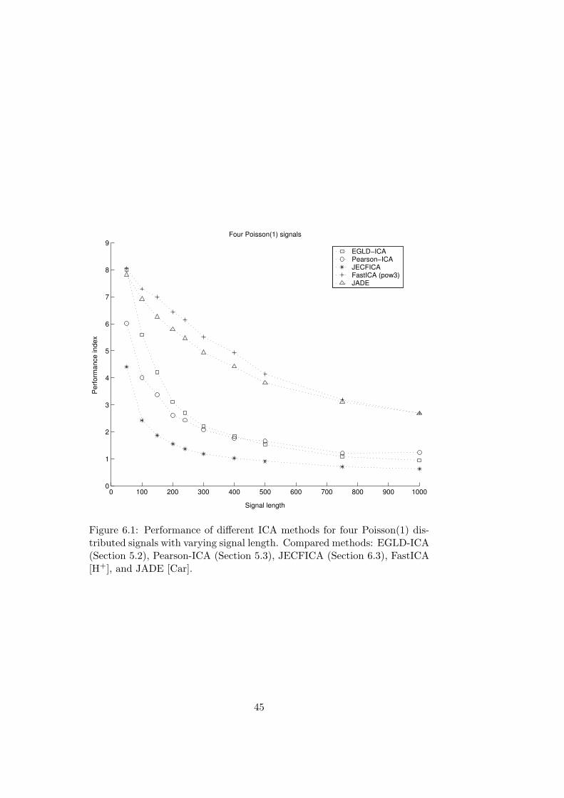
0 100 200 300 400 500 600 700 800 900 10000

1

2

3

4

5

6

7

8

9

Signal length

Per

form

ance

inde

x

Four Poisson(1) signals

EGLD−ICAPearson−ICAJECFICAFastICA (pow3)JADE

Figure 6.1: Performance of different ICA methods for four Poisson(1) dis-tributed signals with varying signal length. Compared methods: EGLD-ICA(Section 5.2), Pearson-ICA (Section 5.3), JECFICA (Section 6.3), FastICA[H+], and JADE [Car].

45

EGLD−ICA Pearson−ICA JECFICA FastICA (pow3) JADE

0

2

4

6

8

10

12

Four Poisson(1) signals, signal length 500

Per

form

ance

inde

x

ICA method

Figure 6.2: Performance of different ICA methods for four Poisson(1) dis-tributed signals with signal length 500. Compared methods: EGLD-ICA(Section 5.2), Pearson-ICA (Section 5.3), JECFICA (Section 6.3), FastICA[H+], and JADE [Car].

46

Chapter 7

Conclusion

7.1 Summary

This thesis addressed the problem of blind signal separation using inde-pendent component analysis (ICA). These methods allow solving many dif-ficult signal processing problems in different application domains. Blindtechniques are very important in applications for which there are sets ofrecorded data or observations, but exact details of the system which pro-duced the observations are unknown. The ICA-based methods have shownto be very successful blind approach.

In this thesis, the theoretical conditions for the traditional linear ICAmodel to qualify as blind separation model were established. It was shownthat it is both sufficient and necessary that the mixing matrix is of fullcolumn rank and that there is at most one Gaussian source signal. It was alsoshown that for identifying the mixing matrix it is enough to have no Gaussiansignals no matter how many sources signals there are for a given number ofsensors. This gives conditions for the linear ICA techniques to be used asa blind system identification methods. Additionally, a stronger concept ofuniqueness applying also to the cases where there are more source signalsthan sensors was introduced. Uniqueness quantifies the situations whereICA models could be used to develop blind signal extraction techniqueswhen there are more sources than sensors. Sufficient conditions were alsofound for uniqueness.

The results of the real-valued linear ICA models were extended into twodirections. First, the conditions for separability, identifiability, and unique-ness were derived for the models with complex-valued signals. Separabilitycondition was again shown to be both sufficient and necessary. Surprisingly,in a complex case, some Gaussian signal mixtures were shown to be separa-ble. In order to establish this result, a novel characterization of second-orderstatistics of complex random vectors and decomposition of complex normalrandom vectors were derived. Second, the real-valued linear models were

47

extended to nonlinear mixing models by introducing a class of nonlinearmodels. These models were shown to be separable, and a generic separa-tion technique was proposed. An instance of this model class was appliedsuccessfully to an image enhancement problem.

Finally, two different types of techniques for blind source separationbased on ICA were proposed in this thesis. In the first approach, sourceadaptation was proposed as a method for separation. The EGLD familyof distributions and the Pearson system were used as a flexible models forsource distributions. The strength of these parametric families is that theymodel a wide class of source distributions, including asymmetric distribu-tions, while the estimation of the parameters is still a relatively simple pro-cedure. In the second approach, the idea was to measure directly stochasticindependence of the signals instead of trying to model the sources. It wasshown that characteristic functions provide a criterion quantifying the inde-pendence for all distributions. Furthermore, the terms in the expression arerelatively easily estimated. Based on this expression, an objective functionwas proposed. It was recently shown to be consistent [CB04] and therebyit guarantees a good performance. Finally, an algorithm for relatively fastminimization of the consistent objective function was derived.

7.2 Future work

The linear real-valued ICA model as a tool for blind separation has beenextensively studied over the past fifteen years. The methods presented inthis thesis are highly reliable for all type of sources while still being rela-tively fast. Thus, it is natural to consider this basic separation of instanta-neous mixtures of real-values sources a relatively well-understood problemwith feasible solutions. However, there are relatively few ICA techniquesfor blind identification and even fewer for blind source extraction for theunderdetermined case. These techniques should have a huge demand insome application areas, e.g. in communications. The development of thesemethods ought to get more attention in the future. A possible option is tobase these methods on moment generating functions as noted in the end ofChapter 3.

Surprisingly, only few authors have considered directly the linear instan-taneous ICA model in the complex domain. Since it was shown in this thesisthat the complex-valued ICA models are also well-defined, a reliable sepa-ration of complex mixtures should be possible. An interesting option wouldbe an extension of the characteristic function based techniques to complexsignals.

Nonlinear ICA models have so far found only few applications. This ismore likely due to the fact that nonlinear methods are relatively unknownand difficult to analyse than due to the lack of possible applications. Nonlin-

48

ear models proposed in this thesis should cover many situations of practicalinterest. However, they might be more appealing if the methods developedwould be more flexible to the exact knowledge of the system structure. Asnoted in the end of Chapter 4, a possibility is to form hierarchical para-metric models from individual addition theorem models. The developmentof separation methods for such models is a challenging task. However, oneshould benefit greatly from ideas used to develop separating algorithms forPNL mixtures.

49

Bibliography

[Ach03] S. Achard. Mesures de dependance pour la separation aveuglede sources. PhD thesis, L’Universite Joseph Fourier (GrenobleI), 2003. (In French).

[ACY96] S. Amari, A. Cichocki, and H. Yang. A new learning algorithmfor blind signal separation. In D. Touretsky, M. Mozer, andH. Hasselmo, editors, Advances in Neural Information Pro-cessing Systems 8, pages 757–763. MIT Press, 1996.

[Acz66] J. Aczel. Lectures on Functional Equations and Their Appli-cations. Academic Press, New York, NY, 1966.

[AGL96a] P.O. Amblard, M. Gaeta, and J.L. Lacoume. Statistics forcomplex variables and signals – Part I: Variables. Signal Pro-cessing, 53:1–13, 1996.

[AGL96b] P.O. Amblard, M. Gaeta, and J.L. Lacoume. Statistics forcomplex variables and signals – Part II: signals. Signal Pro-cessing, 53:15–25, 1996.

[APJ03] S. Achard, D.T. Pham, and C. Jutten. Quadratic dependencemeasure for nonlinear Blind Source Separation. In Proc. of the4th Int. Symposium on ICA and BSS, pages 263–268, Nara,Japan, April 2003.

[ASM03] J. Anemuller, T.J. Sejnowski, and S. Makeig. Complexindependent component analysis of frequency-domain elec-troencephalographic data. Neural Networks, 16(9):1311–1323,November 2003.

[BAMCM97] A. Belouchrani, K. Abed-Meraim, J.-F. Cardoso, andE. Moulines. A blind source separation technique us-ing second-order statistics. IEEE Trans. Signal Processing,45(2):434, February 1997.

[BH00] E. Bingham and A. Hyvarinen. A fast fixed-point algorithmfor independent component analysis of complex valued signals.Int. J. Neural Systems, 10(1):1–8, February 2000.

50

[BJ02] F.R. Bach and M.I. Jordan. Kernel independent componentanalysis. J. Machine Learning Research, 3:1–48, July 2002.

[BPR04] R. Boscolo, H. Pan, and V.P. Roychowdhury. Independentcomponent analysis based on nonparametric density estima-tion. IEEE Trans. Neural Networks, 15(1):55–65, January2004.

[Bre92] L. Breiman. Probability. Classics in Applied Mathematics.SIAM, 1992.

[BS95] A.J. Bell and T.J. Sejnowski. An information maximizationapproach to blind separation and blind deconvolution. NeuralComputation, 7(6):1129–1159, November 1995.

[BZ02] M. Babaie-Zadeh. On blind source separation in convolutiveand nonlinear mixtures. PhD thesis, INPG, Grenoble, France,2002.

[BZJN02] M. Babaie-Zadeh, C. Jutten, and K. Nayebi. A geometricapproach for separating post non-linear mixtures. In Proc.of XI European Signal Processing Conference, pages 11–14,Toulouse, France, September 2002.

[BZP00] Y. Blanco, S. Zazo, and J. Principe. Alternative statisticalGaussianity measure using the cumulative density function.In Proc. of the 2nd Int. Workshop on ICA and BSS, pages537–542, Helsinki, Finland, June 2000.

[CA02] A. Cichocki and S. Amari. Adaptive Blind Signal and Im-age Processing: Learning Algorithms and Applications. JohnWiley & Sons, 2002.

[Car] J.-F. Cardoso. JADE algorithm. Matlab code with references.http://www.tsi.enst.fr/∼cardoso/stuff.html.

[Car93] J-F. Cardoso. An efficient technique for the blind separation ofcomplex sources. In Proc. of the IEEE Signal Proc. Workshopon Higher-Order Statistics, pages 275–279, South Lake Tahoe,CA, June 1993.

[Car96] J.-F. Cardoso. Jacobi angles for simultaneous diagonalization.SIAM J. Matrix Anal. Appl., 17(1):161–164, January 1996.

[Car98] J.-F. Cardoso. Blind signal separation: Statistical principles.Proc. IEEE, 86(10):2009–2025, October 1998.

51

[Car99] J.-F. Cardoso. Higher-order contrast for independent compo-nent analysis. Neural Computation, 11(1):157–192, January1999.

[CB04] A. Chen and P.J. Bickel. Consistent independent componentanalysis and prewhitening. IEEE Trans. Signal Processing,February 2004. Submitted.

[CCA00] S. Choi, A. Cichocki, and S. Amari. Flexible independentcomponent analysis. J. VLSI Signal Processing, 26(1/2):25–38, 2000.

[CL96] J.-F. Cardoso and B. H. Laheld. Equivariant adaptive sourcesaparation. IEEE Trans. Signal Processing, 44(12):3017–3030,December 1996.

[CM99] J. Cao and M. Murata. A stable and robust ica algorithmbased on t-distribution and generalized gaussian distributionmodels. In Proc. of the IEEE Signal Proc. Society Work-shop on Neural Networks for Signal Processing, pages 283–292,Madison, WI, August 1999.

[Com94] P. Comon. Independent component analysis, a new concept?Signal Processing, 36(3):287–314, April 1994.

[Com04] P. Comon. Blind identification and source separation in 2x3under-determined mixtures. IEEE Trans. Signal Processing,52(1):11–22, January 2004.

[CS93] J.-F. Cardoso and A. Souloumiac. Blind beamforming for non-gaussian signals. IEE Proceedings-F, 140(6):362–370, Decem-ber 1993.

[Cso81] S. Csorgo. Multivariate empirical characteristic functions.Zeitschrift fur Wahrscheinlichkeitstheorie und verwandte Ge-biete, 55:203–229, 1981.

[CT91] T.M. Cover and J.A. Thomas. Elements of Information The-ory. John Wiley & Sons, 1991.

[Cup75] R. Cuppens. Decomposition of Multivariate Probabilities, vol-ume 29 of Probability and Mathematical Statistics. AcademicPress, New York, NY, 1975.

[CUR94] A. Cichocki, R. Unbehauen, and E. Rummert. Robust learningalgorithm for blind source separation of signals. ElectronicsLetters, 30(17):1386–1387, August 1994.

52

[DAK00] S.C. Douglas, S. Amari, and S.-Y. Kung. On gradient adap-tation with unit-norm constraints. IEEE Trans. Signal Pro-cessing, 48(6):1843–1847, June 2000.

[DK96] E.J. Dudewicz and Z.A. Karian. The extended generalizedlambda distribution (EGLD) system for fitting distributionsto data with moments, II: Tables. Amer. J. of Math. Manage-ment Sci., 16(3 & 4):271–332, 1996.

[DL95] N. Delfosse and P. Loubaton. Adaptive blind separation ofindependent sources: a deflation approach. Signal Processing,45(1):59–83, July 1995.

[Dou00] S.C. Douglas. Self-stabilized gradient algorithms for blindsource separation with orthogonality constraints. IEEE Trans.Neural Networks, 11(6):1490–1497, November 2000.

[DT00] G.A. Darbellay and P. Tichavsky. Independent componentanalysis through direct estimation of the mutual information.In Proc. of the 2nd Int. Workshop on ICA and BSS, pages69–74, Helsinki, Finland, June 2000.

[EAS98] A. Edelman, T.A. Arias, and S.T. Smith. The geometry ofalgorithms with orthogonality constraints. SIAM J. MatrixAnal. Appl., 20(2):303–353, 1998.

[Feu93] A. Feuerverger. A consistent test for bivariate dependence.International Statistical Review, 61(3):419–433, 1993.

[Fio03] S. Fiori. Extended hebbian learning for blind separationof complex-valued sources. IEEE Trans. Circuits Syst. II,50(4):195–202, April 2003.

[GC98] O. Grellier and P. Comon. Blind separation of discrete sources.IEEE Signal Processing Lett., 5(8):212–214, August 1998.

[GL89] G.H. Golub and C.F.V. Loan. Matrix computations. TheJohns Hopkins University Press, 2nd edition, 1989.

[Gol73] A.A. Goldberg. On a problem of Ju. V. Linnik. Soviet Math.Dokl., 14(4):950–953, 1973.

[Gra90] R.M. Gray. Entropy and Information Theory. Springer-Verlag,New York, NY, 1990.

[H+] A. Hyvarinen et al. FastICA algorithm. Matlab code withreferences. http://www.cis.hut.fi/projects/ica/fastica/.

53

[Hay96] S. Haykin. Adaptive Filter Theory. Prentice Hall, 3rd edition,1996.

[Hay00] S. Haykin, editor. Unsupervised Adaptive Filtering: Vol. 1:Blind Source Separation. Wiley, 2000.

[HKO01] A. Hyvarinen, J. Karhunen, and E. Oja. Independent Compo-nent Analysis. John Wiley & Sons, 2001.

[HL] C.T. Hill and M.L. Lederman. Teaching symmetryin the introduction physics curriculum. Online article.http://www.emmynoether.com/.

[HO97] A. Hyvarinen and E. Oja. A fast fixed-point algorithmfor independent component analysis. Neural Computation,9(7):1483–1492, 1997.

[HP99] A. Hyvarinen and P. Pajunen. Nonlinear independent com-ponent analysis: Existence and uniqueness results. NeuralNetworks, 12(3):429–439, April 1999.

[JBZH04] C. Juttan, M. Babaie-Zadeh, and S. Hosseini. Three easyways for separating nonlinear mixtures? Signal Processing,84(2):217–229, February 2004.

[JK03] C. Jutten and J. Karhunen. Advances in nonlinear blindsource separation. In Proc. of the 4th Int. Symposium on ICAand BSS, pages 245–256, Nara, Japan, April 2003.

[Jut87] C. Jutten. Calcul neuromimetique et traitment du signal, anal-yse en composantes independantes. PhD thesis, INPG, Uni-versity of Grenoble, France, 1987. (In French).

[Kan95] A. Kankainen. Consistent Testing of Total IndependenceBased on Empirical Characteristic Function. PhD thesis, Uni-versity of Jyvaskyla, Finland, 1995.

[KDM96] Z.A. Karian, E.J. Dudewicz, and P. McDonald. The extendedgeneralized lambda distribution system for fitting distribu-tions to data: history, completion of theory, tables, applica-tions, the “final word” on moment fits. Comm. in Statistics:Simulation and Computation, 25(3):611–642, 1996.

[KK02] J. Karvanen and V. Koivunen. Blind separation methodsbased on pearson system and its extensions. Signal Processing,82(4):663–673, April 2002.

54

[KLR73] A.M. Kagan, Yu.V. Linnik, and C.R. Rao. CharacterizationProblems in Mathematical Statistics. Probability and Mathe-matical Statistics. John Wiley & Sons, New York, NY, 1973.

[KM99] R.R. King and H. MacGillivray. A starship method for thegeneralized lambda distributions. Australian New Zealand J.Statistics, 41(3):353–374, 1999.

[KU98] A. Kankainen and N.G. Ushakov. Consistent modification ofa test for independence based on the empirical characteristicfunctions. Journal of Mathematical Sciences, 89(5):1486–1493,1998.

[Kul68] S. Kullback. Information Theory and Statistics. Dover Publi-cations, Inc., New York, NY, reprint edition, 1968.

[LLS99] T-W. Lee, M.S. Lewicki, and T.J. Sejnowski. Blind source sep-aration of more sources than mixtures using overcomplete rep-resentations. IEEE Signal Processing Lett., 6(4):87–90, April1999.

[LMVC03] L. De Lathauwer, B. De Moor, J. Vandewalle, and J.-F. Car-doso. Independent component analysis of largely underdeter-mined mixtures. In Proc. of the 4th Int. Symposium on ICAand BSS, pages 29–33, Nara, Japan, April 2003.

[LO77] Yu.V. Linnik and I.V. Ostrovskii. Decomposition of RandomVariables and Vectors, volume 48 of Translation of Mathemat-ical Monographs. AMS, 1977.

[Lue73] D.G. Luenberger. Introduction to Linear and Nonlinear Pro-gramming. Addison-Wesley, Reading, MA, 1973.

[Luk70] E. Lukacs. Characteristic Functions. Griffin, London, GreatBritain, second edition, 1970.

[LY03] Y. Lomnitz and A. Yeredor. A blind-ML scheme for blindsource separation. In Proc. of the 2003 IEEE Workshop onStatistical Signal Processing, pages 581–584, St. Louis, MO,October 2003.

[Man02] J.H. Manton. Optimization algorithms exploiting unitaryconstraints. IEEE Trans. Signal Processing, 50(3):635–650,March 2002.

[MD02] H. Mathis and S.C. Douglas. On the existence of universalnonlinearities for blind source separation. IEEE Trans. SignalProcessing, 50(5):1007–1016, May 2002.

55

[MI03] E.G. Miller and J.W. Fisher III. Independent compo-nents analysis by direct entropy minimization. Report No.UCB/CSD-3-1221, University of California, Berkeley, CA,January 2003.

[Mor01] E. Moreau. A generalization of joint-diagonalization crite-ria for source separation. IEEE Trans. Signal Processing,49(3):530–541, March 2001.

[NM93] F.D. Neeser and J.L. Massey. Proper complex random pro-cesses with applications to information theory. IEEE Trans.Inform. Theory, 39(4):1293–1302, July 1993.

[NS95] C.L. Nikias and M. Shao. Signal Processing with α-StableDistributions and Applications. Wiley, New York, NY, 1995.

[OS89] A.V. Oppenheim and R.W. Schafer. Discrete-Time SignalProcessing. Prentice Hall, Englewood Cliffs, NJ, 1989.

[Pan03] L. Paninski. Estimation of entropy and mutual information.Neural Computation, 15(6):1191–1253, June 2003.

[PB97] B. Picinbono and P. Bondon. Second-order statistics of com-plex signals. IEEE Trans. Signal Processing, 45(2):411–420,February 1997.

[PG97] D.T. Pham and P. Garat. Blind separation of mixture of in-dependent sources through a quasi-maximum likelihood ap-proach. IEEE Trans. Signal Processing, 45(7):1712–1725, July1997.

[Pha96] D.T. Pham. Blind separation of instantaneous mixture ofsources via an independent component analysis. IEEE Trans.Signal Processing, 44(11):2768–2779, November 1996.

[Pic96] B. Picinbono. Second-order complex random vectors andnormal distributions. IEEE Trans. Signal Processing,44(10):2637–2640, October 1996.

[PK97] P. Pajunen and J. Karhunen. Blind separation of binarysources with less sensors than sources. In Proc. of the 1997Int. Conference on Neural Networks, pages 1994–1997, Hous-ton, TX, June 1997.

[PM01] J-C. Pesquet and E. Moreau. Cumulant-based independencemeasures for linear mixtures. IEEE Trans. Inform. Theory,47(5):1947–1956, July 2001.

56

[PTVF92] W. Press, S. Teukolsky, W. Vetterling, and B. Flannery. Nu-merical Recipes in C: The Art of Scientific Computing. Cam-bridge University Press, second edition, 1992.

[Sco87] W.R. Scott. Group Theory. Dover Publications, Inc., NewYork, NY, reprint edition, 1987.

[SR00] G.J. Szekely and C.R. Rao. Identifiability of distributionsof independent random variables by linear combination andmoments. Sankhya, Series: A, 62(2):193–202, 2000.

[SS03] P.J. Schreier and L.L. Scharf. Second-order analysis of im-proper complex random vectors and processes. IEEE Trans.Signal Processing, 51(3):714–725, March 2003.

[SY04] A. Smekhov and A. Yeredor. Optimization of JADE using anovel optimally weighted joint diagonalization approach. InProc. of the 2004 European Conference on Signal Processing,Vienna, Austria, September 2004. to appear.

[SYM01] Y. Shereshevski, A. Yeredor, and H. Messer. Super-efficiencyin blind signal separation of symmetric heavy-tailed source. InProc. of the 2001 IEEE Workshop on Statistical Signal Por-cessing (SSP2001), pages 78–81, Singapore, August 2001.

[Tal01a] A. Taleb. An algorithm for the blind identification of n in-dependent signals with 2 sensors. In Proc. of InternationalSymposium on Signal Processing and Its Applications, pages5–8, Kuala Lumpur, Malaysia, August 2001.

[Tal01b] A. Taleb. Source separation in structured nonlinear models.In Proc. of the 26th Int. Conference on Acustics, Speech, andSignal Processing, pages 3513–3516, Salt Lake City, UT, May2001.

[Tal02] A. Taleb. A generic framework for blind source separation instructured nonlinear models. IEEE Trans. Signal Processing,50(8):1819–1830, August 2002.

[TJ99a] A. Taleb and C. Jutten. Batch algorithm for source separationin post-nonlinear mixtures. In Proc. of the First Int. Work-shop on ICA and Signal Separation, pages 155–160, Aussois,France, March 1999.

[TJ99b] A. Taleb and C. Jutten. On underdetermined source separa-tion. In Proc. of the 24th Int. Conference on Acustics, Speech,and Signal Processing, volume 3, pages 1445–1448, Phoenix,AZ, March 1999.

57

[TJ99c] A. Taleb and C. Jutten. Source separation in post-nonlinearmixtures. IEEE Trans. Signal Processing, 47(10):2807–2820,October 1999.

[Tuk60] J.W. Tukey. The practical relationship between the com-mon transformations of percentages of counts and of amounts.Technical Report 36, Statistical Techniques Research Group,Princeton University, 1960.

[Ush99] G. Ushakov. Selected Topics in Characteristic Functions.Modern Probability and Statistics. VSP VB, Utrect, TheNetherlands, 1999.

[VK96] N.N. Vakhania and N.P. Kandelaki. Random vectors withvalues in complex Hilbert spaces. Theory Probab. Appl.,41(1):116–131, February 1996.

[Yer00] A. Yeredor. Blind source separation via the second character-istic function. Signal Processing, 80(5):897–902, May 2000.

[Yer02] A. Yeredor. Non-orthogonal joint diagonalization in the least-squares sense with application in blind source separation.IEEE Trans. Signal Processing, 50(7):1545–1553, July 2002.

58