Consumption Oriented Capital Asset Pricing Model and ...joc.hcc.edu.pk/articlepdf/Idolor Eseoghene...

The Journal of Commerce

Vol.6, No.3 pp.1-22

_______________________________________________________________ * Department of Banking and Finance, University of Benin, Nigeria. GSM: 08032272040,

07025655544, E-Mail: [email protected]; [email protected]

Consumption Oriented Capital Asset Pricing Model

and Capital Asset Pricing Model in the Nigerian

Capital Market: A Comparative Study

Idolor, Eseoghene Joseph *

_______________________________________________________________

Abstract

In this study, we test whether the Consumption Capital Asset Pricing Model (CCAPM) is

superior to the Capital Asset Pricing Model (CAPM) in explaining portfolio returns in the

Nigerian capital market. The data collected for the study ranged from the third quarter (Q3) of

year 2000 to the fourth quarter (Q4) of year 2009. In comparing both CAPM and CCAPM

performance in the Nigerian capital market for the period of study, we conducted descriptive

statistics, unit root test and ordinary least square (OLS) regression. In all, our result shows that

CCAPM is not superior to CAPM in explaining variations in portfolio returns of quoted

companies in the Nigerian capital market. In our results, we observed that both CCAPM and

CAPM with lags can be used for pricing assets (portfolio’s) in the Nigerian capital market.

The use of consumption per head (C/P) in our CCAPM model was shown to be statistically

insignificant in explaining portfolio returns in the Nigerian capital market. On the basis of the

research findings, the study recommends that other measures of consumption proxies should

be used to further test if the more recently developed CCAPM model would be better than

conventional CAPM in explaining portfolio returns of quoted Nigerian companies. This could

include consumption measures like consumption volatility, expectation and surplus, consumer

durables, real estate acquisition and human capital utilization.

Key words: CAPM, CCAPM, Nigerian Stock Exchange, Portfolio Returns, Beta, Risk Free

Rate, Stocks

_______________________________________________________________

Capital Asset Pricing Model in Nigeria 2

Introduction

The behaviour of share prices, and the relationship between risk and return in

financial markets, have long been of interest to researchers. In 1905, a young scientist

named Albert Einstein, seeking to demonstrate the existence of atoms, developed an

elegant theory based on Brownian motion. Einstein explained Brownian motion the

same year he proposed the theory of relativity. At that time his results were

considered completely revolutionary. However, the theory of Brownian motion had

been discovered five years earlier by a young French doctoral candidate named Louis

Bachelier. He, too was trying to explain certain complex movements: stock prices on

the Paris Bouse (Cagnetti, 2001). Bachelier was the first to study the fluctuations in

the prices of stocks and shares and their probability distributions. His Ph.D. thesis

contained remarkable results, which anticipated not only Einstein’s theory of

Brownian motion but also many of the modern concepts of theoretical finance.

Bachelier received a respectable “mention honorable”, but his theory did not receive

much attention and he died in provincial obscurity in 1946 (Holt, 1997). The full

potential of Bachelier’s theory was only realized some 50 years later by Mandelbrot

(1963) and Fama (1965). Their findings that the variance of returns is not constant

over time (heteroscedasticity) and that the distribution of price changes were not

Gaussian but leptokurtic, are among the foundations of modern financial theory.

Fama (1965) concluded that the empirical distributions of share prices followed not a

Gaussian but a Stable Paretian distribution with characteristic exponent less than two

(2), that is, with finite mean but infinite variance.

However, it was only with the Capital Asset Pricing Model (CAPM)

developed by Sharpe (1964) that one of the important problems of modern financial

economics was formalized: the quantification of the trade-off between risk and

expected return. Proponents of the CAPM argue that Beta (β), a measure of

systematic risk relative to the market portfolio, is the sole determinant of return. Any

additional variability caused by events peculiar to the individual asset can be

“diversified away” as capital markets do not reward risks borne unnecessarily

(Cagnetti, 2001). To date numerous versions, extensions and improvements upon the

model have been observed in the empirical literature. They include the old CAPM

model (frought with numerous weaknesses as a result of simplistic assumptions upon

which it is based), the Inter-temporal Capital Asset Pricing Model (ICAPM) and the

Consumption Capital Asset Pricing Model (C-CAPM) to name only a few.

Many attempts have been made to see which of them better

reflects/determine assets prices in numerous developed and emerging markets

Idolor, Eseoghene Joseph 3

worldwide. Analysts have used different related approaches and more tools and

related models are being evolved in the literature to deal with this aspect of asset

pricing. All the attempts are to see if any one particular model or method could prove

to be the most appropriate model for pricing assets and portfolio’s in the capital

markets. In this regard, the Consumption Capital Asset Pricing Model (CCAPM), a

newer variant of the CAPM has attracted latter day analysts and has been adjudged a

possible tool of the future in both developed and developing economies. It has

received a new impetus and is currently at the front burners of capital asset pricing in

the empirical literature. It is against this background that the study test whether

CCAPM is superior to CAPM model in explaining portfolio returns in the Nigerian

capital market.

Capital Asset Pricing Model (CAPM): An Overview

The capital asset pricing model (CAPM) of William Sharpe (1964) and John

Lintner (1965) marks the birth of asset pricing theory (resulting in a Nobel Prize for

Sharpe in 1990). Four decades later, the CAPM is still widely used in applications,

such as estimating the cost of capital for firms and evaluating the performance of

managed portfolios. It is the centerpiece of MBA investment courses. Indeed, it is

often the only asset pricing model taught in these courses (Fama and French, 2004).

The attraction of the CAPM is that it offers powerful and intuitively pleasing

predictions about how to measure risk and the relationship between expected return

and risk. Unfortunately, the empirical record of the model is poor – poor enough to

invalidate the way it is used in applications. The CAPM’s empirical problems may

reflect theoretical failings, the result of many simplifying assumptions. But they may

also be caused by difficulties in implementing valid tests of the model. For example,

the CAPM says that the risk of a stock should be measured relative to a

comprehensive “market portfolio” that in principle can include not just traded

financial assets, but also consumer durables, real estate and human capital. Even if we

take a narrow view of the model and limit its purview to traded and financial assets, is

it legitimate to limit further the market portfolio to common stocks (a typical choice),

or should the market be expanded to include bonds, and other financial assets,

perhaps around the world? In the end, we argue that whether the model’s problems

reflect weaknesses in the theory or in its empirical implementation, the failure of the

CAPM in some empirical tests implies to such researchers that most applications of

the model are invalid, though numerous dissenters still exist.

Indeed, CAPM has been one of the most challenging topics in financial

economics. Almost any manager who wants to undertake a project must justify his


decision partly based on CAPM. The reason is that the model provides the means for

a firm to calculate the return that its investors demand. This model was the first

successful attempt to show how to assess the risk of the cash flows of a potential

investment project, to estimate the project’s cost of capital and the expected rate of

return that investors will demand if they are to invest in the project. The model was

developed to explain the differences in the risk premium across assets. According to

the theory these differences are due to differences in the riskiness of the returns on the

assets. The model states that the correct measure of the riskiness of an asset is its beta

and that the risk premium per unit of riskiness is the same across all assets. Given the

risk free rate and the beta of an asset, the CAPM predicts the expected risk premium

for an asset (Michailidis et al, 2006).

The Logic of the CAPM

The CAPM builds on the model of portfolio choice developed by Harry

Markowitz (1959). In Markowitz’s model, an investor selects a portfolio at time t-1

that produces a stochastic return at t. The model assumes investors are risk averse

and, when choosing among portfolios, they care only about the mean and variance of

their one-period investment return. As a result, investors choose “mean-variance-

efficient” portfolios, in the sense that the portfolios minimize the variance of portfolio

return, given expected return, and maximize expected return, given variance, thus, the

Markowitz approach is often called a “mean-variance model”.

The portfolio model provides an algebraic condition on asset weights in

mean-variance-efficient portfolios. The CAPM turns this algebraic statement into a

testable prediction about the relation between risk and expected return by identifying

a portfolio that must be efficient if asset prices are to clear the market of all assets.

Sharpe (1964) and Lintner (1965) add two key assumptions to the Markowitz model

to identify a portfolio that must be mean-variance-efficient. The first assumption is

complete agreement; given market clearing asset prices at t-1, investors agree on the

joint distribution of asset returns from t-1 to t. and this distribution is the true one –

that is, it is the distribution from which the returns we use to test the model are drawn.

The second assumption is that there is borrowing and lending at a risk-free rate,

which is the same for all investors and does not depend on the amount borrowed or

lent (Fama and French, 2004).

Consumption Capital Asset Pricing Model (CCAPM): A Cursory Overview

In the last section we saw that CAPM identifies the risk of any security as the

covariance between the security's rate of return and the rate of return on the market


portfolio. According to the CAPM, the uncertainty associated with the return on the

market portfolio is the sole source of risk in the economy but CAPM has no

theoretical structure that allows us to readily identify what it is that causes the market

portfolio to be risky. Macroeconomics does have such a theoretical structure. It tells

us, for example, how the profits of firms are related to such things as overall

economic activity (GDP) and the government's conduct of monetary and fiscal

policies. Macroeconomics provides us with models that enable us to not only identify

various sources of aggregate uncertainty but to also understand the mechanisms by

which these affect security returns and prices.

The asset pricing model that is embedded in stochastic models of

macroeconomics is called the Consumption Based Asset Pricing Model (CCAPM).

The name derives from the fact that the equations that describe the behaviour of asset

prices and returns in the CCAPM devolve from the consumption/saving and asset

choice decisions of households. In the CCAPM the economy is assumed to be

populated by a large number of households that are identical in all respects, including

preferences and endowments. This assumption permits decision making to be

analyzed by examining the behaviour of a single, representative household. No

matter what the macroeconomic setting is, one consequence of the CCAPM

assumption that all households are identical is that households will never exchange

assets with one another. For instance it will never be the case that one household will

borrow from another. Why? All households are identical; if one wishes to borrow, all

will wish to borrow and there will be no household that wishes to lend. If there are

any assets that exist in positive net supply, these must come from outside the

household sector (e.g. from governments, businesses, or the rest of world).

Studies are replete on the empirical implications of the consumption-oriented

capital asset pricing model (CCAPM), and its performance when compared with a

model based on market portfolio. These empirical studies are dispersed and primarily

focused on the performance of the model. Working (1960), used, quarterly returns on

assets and the covariance of those returns in the spot consumption rate. He then

derived the relation between the desired population covariance (and betas) of assets

returns relative to changes in interval consumption. The empirical results showed a

variance of interval consumption changes of 0.6667 the variance of spot consumption

changes, while the autocorrelation of interval consumption of 0.25 due to integration

of spot rates was reported. These results were generalized by Tiao (1972) to examine

the empirical performance of CCAPM.


Lambert (1978) and Beaver, Lambert and Morse (1980) have also conducted

empirical research on studies of stock prices and corporate earnings, using similar

result on time aggregation. In other studies, Grossman, Melino and Shiller

(1987) derived maximum likelihood estimated of CCAPM parameters. The empirical

results explicitly accounting for time aggregation of consumption showed that

CCAPM prices assets with respect to changes in aggregate consumption between two

points in time. Marsh (1981) examining an alternative treatment for this

measurement problem postulated a latent variable model to estimate the parameters of

the CCAPM. The results validated the existence of assets return and individuals

optimal consumption paths followed diffusion process. It also indicated that over a

discrete time interval the joint distribution of assets returns and individual

consumption path tends to assume normality. In the same vein, Breeden’s (1979)

derivation of the CCAPM justifies the use of betas measured relative to a portfolio

that has maximum correlation with growth in aggregate consumption, in place of

betas measured relative to aggregate consumption (Igbinovia and Uwubanmwen,

2012).

Exploring the implications of the CCAPM for a long sample period requires

aggregate consumption data from different source. As a result of the difficulty in

generating consumption data, which is not easy to come by, different researchers

have been faced with the problem of measured consumption. Particularly, aggregate

consumption data are not available except expenditures on non durables, Plus

services, following Hall (1978). Basically, four measurement problems are associated

with measured consumption. These problems are; reporting of expenditures rather

than consumption (the durable problem), the reporting of an integral consumption

rates, rather than the consumption rate at a point in time, infrequent reporting of

consumption data relative to stock returns, and the problem of pure sampling error in

consumption measures. This is because only a subset of the total population of

consumption transaction is measured (Igbinovia and Uwubanmwen, 2012).

These measured problem have greatly limited the empirical robustness of

CCAPM results and have led researchers to adopt varied econometric measuring

techniques in order to minimize the problem, since the returns on many capital assets

are available for a longer time and are reported more frequently than consumption.

More precise evidence on the CCAPM can be provided if only returns were needed to

empirically validate the theory. Since this is not the case, much controversy still

exists in the empirical literature.


CCAPM and CAPM: A Comparison

Breeden (1979) and Lucas (1978) provided the foundation of the

Consumption Capital Asset Pricing Model (CCAPM) leading to the award of a Nobel

Laureate in economics to one of them. Their model is an extension of the traditional

capital asset pricing model CAPM. It is best used as a theoretical model, but it can

help to make sense of variation in financial asset returns over time and in some cases,

its results can be relevant than those achieved through the CAPM model. While the

CAPM relies on the market portfolio return in order to understand and predict future

asset prices, the CCAPM relies on the aggregate consumption. In the CAPM, risky

assets create uncertainty in an investors wealth, which is determined by the market

which creates uncertainty in consumption. What an investor will spend becomes

uncertain because his or her wealth is uncertain as a result of a decision to invest in

risky assets (Igbinovia and Uwubanmwen, 2012).

The CCAPM prices assets with respect to changes in aggregate consumption

between two points in time. In contrast, the available data on aggregate consumption

provide total expenditure on goods and services over a period of time. These

differences between consumption in theory and its measured counterpart suggest the

first two problems. First, goods and services need not be consumed in the same

period that they are purchased.

Second measured aggregate consumption is closer to an integral of

consumption over a period of time than to “Spot” consumption (at a point in time).

The “Spot” consumption is also known as instantaneous consumption. The second

problem creates a “summation bias”. In a more succinct term, the CCAPM is based

on the notion that the aggregate capital consumption and return on all assets tend to

follow an optimal path of normal distribution.

On the other hand, the capital asset pricing model (CAPM) is a market

oriented capital asset pricing model. The CAPM model by Sharpe (1964) used the

beta coefficient to ascertain the riskiness of stock. A beta coefficient equal to one

indicates that a particular stock or capital asset has the same amount of systematic

risk with the entire portfolio of securities. Hence there would be no need to adjust the

portfolio. If all securities in the portfolio have unitary beta coefficients, equilibrium is

attained and security prices are rational with little tendency to fluctuate. On the other

hand, a beta coefficient greater than unity indicates that the security in question has

become riskier, while a coefficient less than unity implies that the security has

become safer. These cases are deviations from equilibrium position, which imply that

security prices would also be out of equilibrium values.


According to Sharpe (1964), this price behavior could also be viewed from

the perspective of expected returns on the security and the covariance of such

security. If the covariance is zero, it implies that the price of security reflects the

expected returns on it, which is an equilibrium situation that makes price stable. A

negative covariance depresses the price below the fundamental value, while a positive

covariance would raise it above its fundamental value. The movement of security

price above and below the fundamental value creates speculative transactions that

tend to redirect the price towards equilibrium level. Thus, if the fundamental value

(returns) is higher security price would rise, but it would fall if the value becomes

lower. Thus, while the capital asset pricing model CAPM is market oriented, the

consumption oriented capital asset pricing model is consumption driven.

Methodology and Research Design

Data

The nature of this study necessitated the use of secondary data. The data

include our constructed selected companies stock portfolio returns (i.e. equal

weighting of the changes in share price was used in computing the weighted average

portfolio returns), companies beta and market premium was sourced from Cashcraft

Asset management website while the consumption per head (C/Y) was sourced from

Central Bank of Nigeria (CBN). The quarterly data used in this study ranged from

2000 Q3 to 2009Q4.

Data Analysis Techniques

The econometric techniques adopted in this study include unit root test and

OLS regression analysis. We conducted unit root test based on the possibility of non-

stationarity in the collected time series data. The fundamental justifications for the

less reliance on non-stationary data in this study is that there exist a high tendency for

most time series variables to be non-stationary and OLS results also become spurious

when time series data are non-stationary. In this study we therefore compare the

CAPM and CCAPM under the context of stationary time series data. We also

conducted preliminary statistical analysis such as descriptive statistics. In conducting

this analysis we used EViews 7.0 econometric software. Before estimating the CAPM

and CCAPM models, the dependent and independent variables are separately

subjected to some stationarity test using augmented Dickey fuller (ADF) test.

CAPM Regression Model


This model examines how market premium ( ( ) )m fE R R relates to the

selected quoted companies expected stock returns ( )i

E R using quarterly data;

( ) ( ( ) )i f i m fE R R E R R ………….. (13)

CCAPM Regression model

This model examines how market premium ( ( ) )m fE R R and consumption

per head (C/P) relates to the selected quoted companies expected portfolio returns

( )i

E R using quarterly data;

( ) ( ( ) ) ( / )f m fE R R E R R C P ……….. (13)

Where;

E(Ri) = Expected portfolio returns, this value is computed by taking the log of the

ratio between weighted average current stock price and previous stock prices of the

selected companies. This represent the dependent variable for both the CAPM and

CCAPM regression models.

E = error term.

fR = Risk free rate proxied by Treasury bill rates

( ( ) )m fE R R = Market premium, this is measured as the difference between the

Treasury bill rate and the rate returns of the entire stock market (computed from all

share price index). Apriori, we expect this variable to positively relate to the quoted

companies portfolio returns (+)

C/P = Per capital consumptions sometimes called consumption per head

= coefficient of C/P

i = CAPM beta = this measures firms undiversified risk and can be measured as

covariance between selected companies portfolio returns to overall stock market

returns divided by the square of stock market returns. This coefficient can be easily

obtained from the CAPM regression model. The coefficient shows the impact of

market premium on the portfolio returns.


Empirical Findings

In this study, we compare the conventional CAPM and Consumption-Based

CAPM in explaining our constructed equity portfolio returns. The study uses per capital

consumptions (C/P), selected quoted companies equity portfolio returns

(PORTRETUNS) and market premium (MKPREMIUM) which is the difference

between market returns (MARKRETUN) and Treasury bill rate (TBRATE). The

quarterly data used in this study ranged from 2000 Q3 to 2009 Q4. To this end, this

section of the paper focus on finding out if Consumption-based CAPM is relatively

better in explaining portfolio returns in the Nigerian capital market than the

conventional CAPM. Before explaining the main analysis in this study we first discuss

the trends, descriptive statistics and unit root test of the portfolio returns. The results

obtained are presented and analyzed as follows;

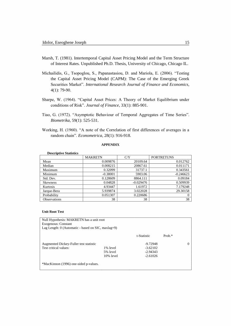
Descriptive Statistics

Figure 1 is a line graph that shows the performance of our constructed

portfolio returns. The graphs show that there is some movement in the portfolio

returns of the sampled companies.

Figure 1: Line graph of portfolio returns

Table 1: Descriptive Statistics of Portfolio returns

Returns Mean Std.

Dev

Skewness Kurtosis Jarque-

Bera

N

PORTRETUNS

0.013

0.092

0.509

7.18

29.3(0.0)

38

Source: Author (2012)

Table 1; shows that the mean value of the portfolio returns of the sampled

quoted companies was 0.013 while the standard deviation was 0.092, the portfolio


returns was positively skewed (0.509) while the kurtosis shows that the portfolio

returns was playtokutic (7.18). The Jaque-bera(JB) test value of 29.3 shows that the

portfolio returns was not normally distributed. This therefore implies that there is

some form of abnormal returns in our constructed portfolio.

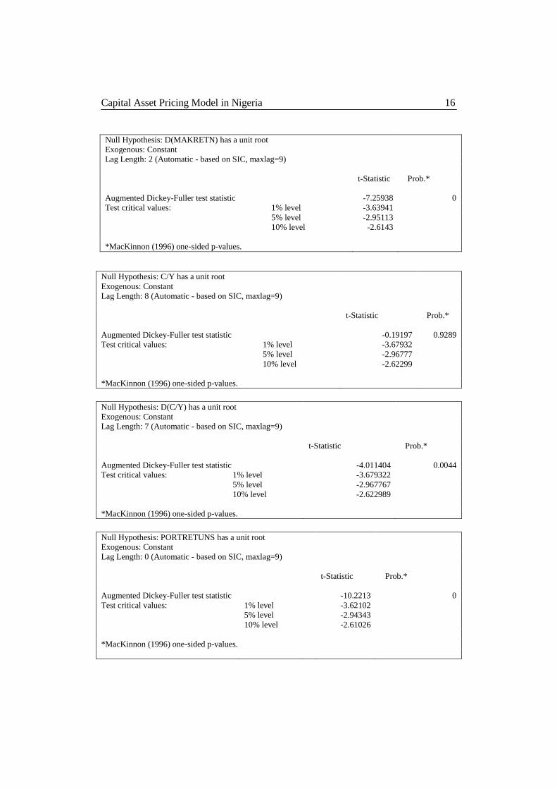
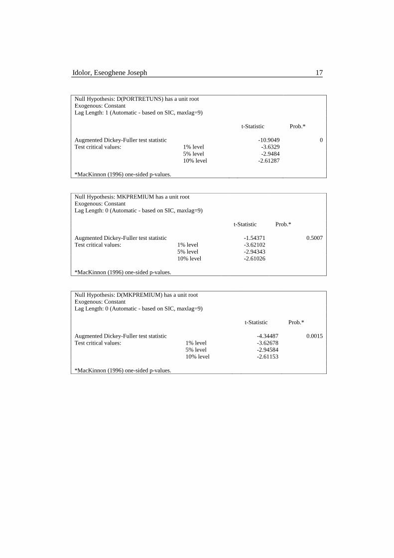
Unit Roots

The unit root test based on the ADF was conducted in this study to identify

the variables order of integration and to find weather its’ best studying their

relationship at levels or first difference. This is shown in Table 2.

Table 2: Unit Root results

Variables ADF Remark

MKPREMIUM

Level -1.54

Stationary

First difference -4.34*

PORTRETUNS

C/P

5% critical value

Level

First Difference

5% critical value

Level

First Difference

5% critical value

-2.95

-10.22*

-10.90*

-2.95

-0.19

-4.011*

-2.97

Stationary

Stationary *significant at 5% levels

The unit root results based on ADF reveal that market premium

(MKPREMIUM) and consumptions per head (C/P) where not stationary at levels

since their ADF statistic at levels where less than the ADF 5% critical values in

absolute term. At first difference all the variable becomes stationary. This therefore

implies that the CAPM and CCAPM would be best compared using a first difference

regression model. The Augmented Dickey-Fuller (ADF) Unit Root test results for the

time series is also presented in Table 2.


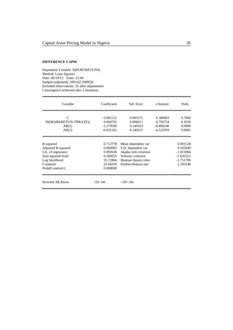
Regression Results

Table 3: CAPM and Consumption CAPM Regression Results

Variables CAPM

MODEL

Consumption CAPM

MODEL

C

∆(C/P)

∆(MKPREMIUM)

AR(1)

AR(2)

0.002

(0.38)

-

-

0.004

(0.79)

-1.18

(-8.41)

-0.64

(-4.52)

0.001

(0.10)

0.00001

(0.17)

0.005

(0.75)

-1.18

(-8.28)

-0.63

(-4.45)

Adj R

F-statistic

DW

AIC

SBC

0.68

25.6(0.0)

2.18

-1.81

-1.64

0.67

18.6(0.0)

2.18

-1.76

-1.53

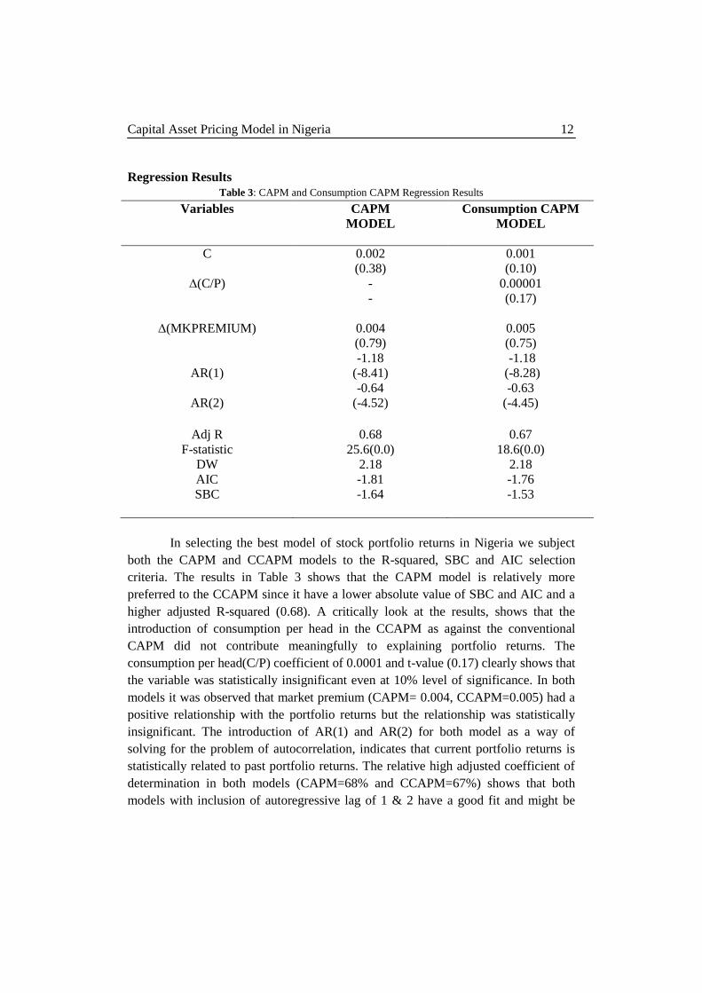
In selecting the best model of stock portfolio returns in Nigeria we subject

both the CAPM and CCAPM models to the R-squared, SBC and AIC selection

criteria. The results in Table 3 shows that the CAPM model is relatively more

preferred to the CCAPM since it have a lower absolute value of SBC and AIC and a

higher adjusted R-squared (0.68). A critically look at the results, shows that the

introduction of consumption per head in the CCAPM as against the conventional

CAPM did not contribute meaningfully to explaining portfolio returns. The

consumption per head(C/P) coefficient of 0.0001 and t-value (0.17) clearly shows that

the variable was statistically insignificant even at 10% level of significance. In both

models it was observed that market premium (CAPM= 0.004, CCAPM=0.005) had a

positive relationship with the portfolio returns but the relationship was statistically

insignificant. The introduction of AR(1) and AR(2) for both model as a way of

solving for the problem of autocorrelation, indicates that current portfolio returns is

statistically related to past portfolio returns. The relative high adjusted coefficient of

determination in both models (CAPM=68% and CCAPM=67%) shows that both

models with inclusion of autoregressive lag of 1 & 2 have a good fit and might be


relatively relevant for portfolio returns prediction. The F-statistics for both models at

1% level was statistically significant.

Following the above, the conclusions from our empirical analysis that are

specific to the aim of our study are outlined as follows;

1. CCAPM is not superior to CAPM in explaining variations in portfolio returns of

quoted companies in Nigeria capital market. Though its results seem better, there

is no clear statistically significant difference upon which to arrive at any form of

valid conclusion to the contrary.

2. Both CCAPM and CAPM with lags can be used for pricing asset portfolio in the

Nigerian capital market

3. The use of consumption per head (C/P) in CCAPM is statistically insignificant in

explaining portfolio returns in the Nigerian capital market. This study on the

basis of our finding suggests that other measures of consumption proxy should be

used to test if the CCAPM would explain returns better than the conventional

CAPM. This could include consumption measures like consumption volatility,

expectation, surplus, consumer durables, real estate acquisition and human capital

utilization. This could be the basis for future research.

Researchers’ Conclusion

The study attempted to determine on a comparative basis if CCAPM is

superior to the more traditional CAPM using a pool of locally available data in the

Nigerian capital market. The whole essence was to determine if the CCAPM will

yield superior results compared to the CAPM when subjected to locally available

Nigerian data. This expectation was not justified from our empirical findings. The

results suggests that while both the CAPM and CCAPM can be used for pricing

assets in the Nigerian bourse, the CCAPM is not statistically superior to CAPM in

explaining variations in portfolio returns of publicly quoted Nigerian companies.

While suggesting that this research work expresses a highly intelligent guide in

comparing the CCAPM with the older CAPM model in the Nigerian bourse (Stock

Exchange); interested researchers are hereby advised to conduct more research on this

area, as improvements will be highly appreciated.

References

Beaver, W., Lambert, R. and Morse, D. (1980). “The Information Content of Security

Prices”. Journal of Accounting and Economics, 2(1): 3-28.


Breeden, D. (1979). An Intertemporal Asset Pricing Model with Stochastic

Consumption and Investment Opportunities. Journal of Financial Economics,

7(1): 265-296.

Cagnetti, A. (2001). Capital Asset Pricing Model and Arbitrage Pricing Theory in the

Italian Stock Market: An Empirical Study. Edinburgh: Management School and

Economics, the University of Edinburgh.

Fama, E.F. (1965). “The Behaviour of Stock Market Prices”. Journal of Business,

38(1): 34-105.

Fama, E.F. and French, K.R. (2004). “The Capital Asset Pricing Model: Theory and

Evidence”. Journal of Economic Perspectives, 18(3): 25-46.

Grossman, S., Melino, A. and Shiller, R. (1987). Estimating the Continuous-Time

Consumption-based Asset-Pricing Model. Journal of Business and Economic

Statistics, 5(1): 315-328.

Hall, R. (1978). Stochastic Implications of the Life Cycle-Permanent Income

Hypothesis: Theory and Evidence. Journal of Political Economy, 86(1): 971-

987.

Holt, J. (1997). “Motion Sickness: A Random Walk from Paris to Wall Street”.

Retrieved 4th of May, 2010, from http://www.linguafrance.com

Igbinovia, I.E. and Uwubanmwen, A.E. (2011). “The Consumption – Oriented

Capital Asset Pricing Model: A Cursory Survey of Empirical Literature. ESUT

Journal of Management Sciences, 6(2): 73-83.

Lambert, R. (1979). The time aggregation of Earnings Series. Unpublished

Manuscript, Graduate School of Business, Stanford University, Stanford, CA.

Lintner, J. (1965). “The Valuation of Risk Assets and the Selection of Risky

Investments in Stock Portfolios and Capital Budgets”. Review of Economics and

Statistics, 47(1): 13-37.

Mandelbrot, B. (1963). “The Variation of Certain Speculative Prices”. Journal of

Business, 36(1): 394-419.

Markowitz, H.M. (1952). “Portfolio Selection”. Journal of Finance, 7(1): 77-91.

http://www.linguafrance.com/


Marsh, T. (1981). Intertemporal Capital Asset Pricing Model and the Term Structure

of Interest Rates. Unpublished Ph.D. Thesis, University of Chicago, Chicago IL.

Michailidis, G., Tsopoglou, S., Papanastasiou, D. and Mariola, E. (2006). “Testing

the Capital Asset Pricing Model (CAPM): The Case of the Emerging Greek

Securities Market”. International Research Journal of Finance and Economics,

4(1): 79-90.

Sharpe, W. (1964). “Capital Asset Prices: A Theory of Market Equilibrium under

conditions of Risk”. Journal of Finance, 33(1): 885-901.

Tiao, G. (1972). “Asymptotic Behaviour of Temporal Aggregates of Time Series”.

Biometrika, 59(1): 525-531.

Working, H. (1960). “A note of the Correlation of first differences of averages in a

random chain”. Econometrica, 28(1): 916-918.

APPENDIX

Descriptive Statistics

MAKRETN C/Y PORTRETUNS

Mean 0.009876 20109.64 0.012762

Median 0.008215 20867.61 0.011171

Maximum 0.32099 31737.1 0.343561

Minimum -0.38001 5903.06 -0.246623

Std. Dev. 0.128609 8864.111 0.09184

Skewness 0.04828 -0.029476 0.509939

Kurtosis 4.93447 1.61972 7.179248

Jarque-Bera 5.939874 3.022028 29.30158

Probability 0.051307 0.220686 0

Observations 38 38 38

Unit Root Test

Null Hypothesis: MAKRETN has a unit root

Exogenous: Constant

Lag Length: 0 (Automatic - based on SIC, maxlag=9)

t-Statistic Prob.*

Augmented Dickey-Fuller test statistic

-9.72948 0

Test critical values: 1% level

-3.62102

5% level

-2.94343

10% level

-2.61026

*MacKinnon (1996) one-sided p-values.


Null Hypothesis: D(MAKRETN) has a unit root

Exogenous: Constant


t-Statistic Prob.*


-7.25938 0


-3.63941

5% level

-2.95113

10% level

-2.6143


Null Hypothesis: C/Y has a unit root

Exogenous: Constant


t-Statistic Prob.*


-0.19197 0.9289


-3.67932

5% level

-2.96777

10% level

-2.62299


Null Hypothesis: D(C/Y) has a unit root

Exogenous: Constant


t-Statistic Prob.*

Augmented Dickey-Fuller test statistic -4.011404 0.0044


-3.679322

5% level

-2.967767

10% level

-2.622989


Null Hypothesis: PORTRETUNS has a unit root

Exogenous: Constant


t-Statistic Prob.*

Augmented Dickey-Fuller test statistic -10.2213 0

Test critical values: 1% level -3.62102

5% level -2.94343

10% level -2.61026



Null Hypothesis: D(PORTRETUNS) has a unit root

Exogenous: Constant


t-Statistic Prob.*


-10.9049 0


-3.6329

5% level

-2.9484

10% level

-2.61287


Null Hypothesis: MKPREMIUM has a unit root

Exogenous: Constant


t-Statistic Prob.*


-1.54371 0.5007


-3.62102

5% level

-2.94343

10% level

-2.61026


Null Hypothesis: D(MKPREMIUM) has a unit root

Exogenous: Constant


t-Statistic Prob.*


-4.34487 0.0015


-3.62678

5% level

-2.94584

10% level

-2.61153



DIFFERENCE CAPM

Dependent Variable: D(PORTRETUNS)

Method: Least Squares

Date: 09/19/12 Time: 23:44

Sample (adjusted): 2001Q2 2009Q4

Included observations: 35 after adjustments

Convergence achieved after 5 iterations

Variable Coefficient Std. Error t-Statistic Prob.

C 0.002121 0.005571 0.380683 0.7060

D((MARKRETUN-TBRATE)) 0.004765 0.006011 0.792754 0.4339

AR(1) -1.179590 0.140323 -8.406246 0.0000

AR(2) -0.635161 0.140337 -4.525959 0.0001

R-squared 0.712778 Mean dependent var 0.001528

Adjusted R-squared 0.684982 S.D. dependent var 0.165049

S.E. of regression 0.092636 Akaike info criterion -1.813066

Sum squared resid 0.266025 Schwarz criterion -1.635312

Log likelihood 35.72866 Hannan-Quinn criter. -1.751706

F-statistic 25.64350 Durbin-Watson stat 2.183146

Prob(F-statistic) 0.000000

Inverted AR Roots -.59-.54i -.59+.54i


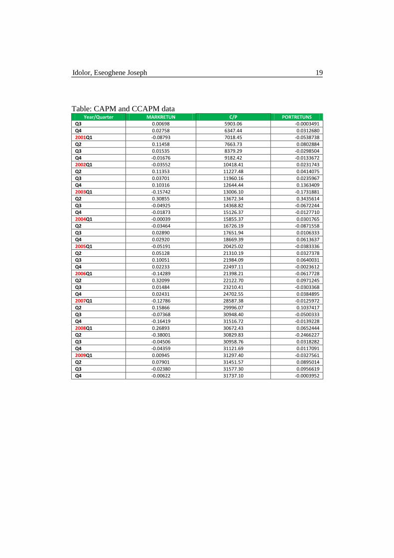
Table: CAPM and CCAPM data Year/Quarter MARKRETUN C/P PORTRETUNS

Q3 0.00698 5903.06 -0.0003491

Q4 0.02758 6347.44 0.0312680

2001Q1 -0.08793 7018.45 -0.0538738

Q2 0.11458 7663.73 0.0802884

Q3 0.01535 8379.29 -0.0298504

Q4 -0.01676 9182.42 -0.0133672

2002Q1 -0.03552 10418.41 0.0231743

Q2 0.11353 11227.48 0.0414075

Q3 0.03701 11960.16 0.0235967

Q4 0.10316 12644.44 0.1363409

2003Q1 -0.15742 13006.10 -0.1731881

Q2 0.30855 13672.34 0.3435614

Q3 -0.04925 14368.82 -0.0672244

Q4 -0.01873 15126.37 -0.0127710

2004Q1 -0.00039 15855.37 0.0301765

Q2 -0.03464 16726.19 -0.0871558

Q3 0.02890 17651.94 0.0106333

Q4 0.02920 18669.39 0.0613637

2005Q1 -0.05191 20425.02 -0.0383336

Q2 0.05128 21310.19 0.0327378

Q3 0.10051 21984.09 0.0640031

Q4 0.02233 22497.11 -0.0023612

2006Q1 -0.14289 21398.21 -0.0617728

Q2 0.32099 22122.70 0.0971245

Q3 0.01484 23210.41 -0.0303368

Q4 0.02431 24702.55 0.0384895

2007Q1 -0.12786 28587.38 -0.0125972

Q2 0.15866 29996.07 0.1037417

Q3 -0.07368 30948.40 -0.0500333

Q4 -0.16419 31516.72 -0.0139228

2008Q1 0.26893 30672.43 0.0652444

Q2 -0.38001 30829.83 -0.2466227

Q3 -0.04506 30958.76 0.0318282

Q4 -0.04359 31121.69 0.0117091

2009Q1 0.00945 31297.40 -0.0327561

Q2 0.07901 31451.57 0.0895014

Q3 -0.02380 31577.30 0.0956619

Q4 -0.00622 31737.10 -0.0003952


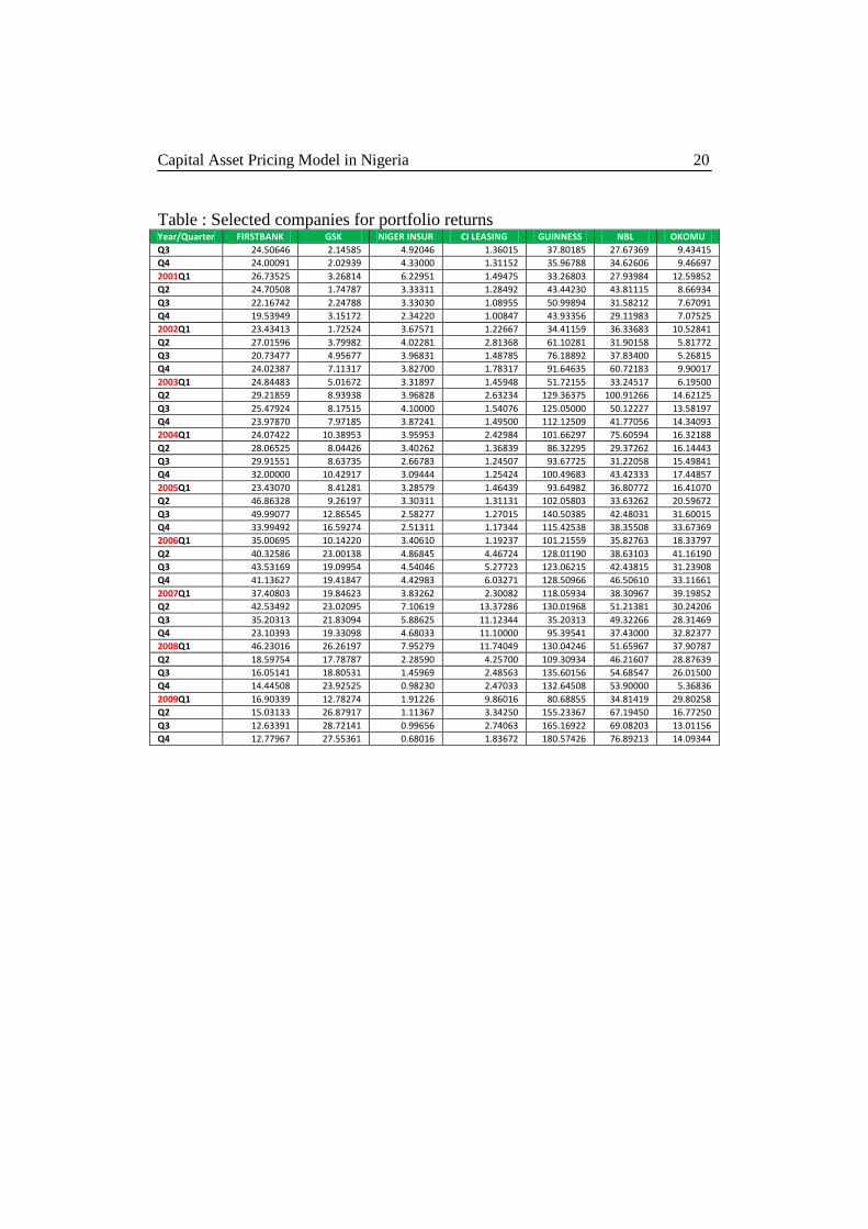
Table : Selected companies for portfolio returns Year/Quarter FIRSTBANK GSK NIGER INSUR CI LEASING GUINNESS NBL OKOMU

Q3 24.50646 2.14585 4.92046 1.36015 37.80185 27.67369 9.43415

Q4 24.00091 2.02939 4.33000 1.31152 35.96788 34.62606 9.46697

2001Q1 26.73525 3.26814 6.22951 1.49475 33.26803 27.93984 12.59852

Q2 24.70508 1.74787 3.33311 1.28492 43.44230 43.81115 8.66934

Q3 22.16742 2.24788 3.33030 1.08955 50.99894 31.58212 7.67091

Q4 19.53949 3.15172 2.34220 1.00847 43.93356 29.11983 7.07525

2002Q1 23.43413 1.72524 3.67571 1.22667 34.41159 36.33683 10.52841

Q2 27.01596 3.79982 4.02281 2.81368 61.10281 31.90158 5.81772

Q3 20.73477 4.95677 3.96831 1.48785 76.18892 37.83400 5.26815

Q4 24.02387 7.11317 3.82700 1.78317 91.64635 60.72183 9.90017

2003Q1 24.84483 5.01672 3.31897 1.45948 51.72155 33.24517 6.19500

Q2 29.21859 8.93938 3.96828 2.63234 129.36375 100.91266 14.62125

Q3 25.47924 8.17515 4.10000 1.54076 125.05000 50.12227 13.58197

Q4 23.97870 7.97185 3.87241 1.49500 112.12509 41.77056 14.34093

2004Q1 24.07422 10.38953 3.95953 2.42984 101.66297 75.60594 16.32188

Q2 28.06525 8.04426 3.40262 1.36839 86.32295 29.37262 16.14443

Q3 29.91551 8.63735 2.66783 1.24507 93.67725 31.22058 15.49841

Q4 32.00000 10.42917 3.09444 1.25424 100.49683 43.42333 17.44857

2005Q1 23.43070 8.41281 3.28579 1.46439 93.64982 36.80772 16.41070

Q2 46.86328 9.26197 3.30311 1.31131 102.05803 33.63262 20.59672

Q3 49.99077 12.86545 2.58277 1.27015 140.50385 42.48031 31.60015

Q4 33.99492 16.59274 2.51311 1.17344 115.42538 38.35508 33.67369

2006Q1 35.00695 10.14220 3.40610 1.19237 101.21559 35.82763 18.33797

Q2 40.32586 23.00138 4.86845 4.46724 128.01190 38.63103 41.16190

Q3 43.53169 19.09954 4.54046 5.27723 123.06215 42.43815 31.23908

Q4 41.13627 19.41847 4.42983 6.03271 128.50966 46.50610 33.11661

2007Q1 37.40803 19.84623 3.83262 2.30082 118.05934 38.30967 39.19852

Q2 42.53492 23.02095 7.10619 13.37286 130.01968 51.21381 30.24206

Q3 35.20313 21.83094 5.88625 11.12344 35.20313 49.32266 28.31469

Q4 23.10393 19.33098 4.68033 11.10000 95.39541 37.43000 32.82377

2008Q1 46.23016 26.26197 7.95279 11.74049 130.04246 51.65967 37.90787

Q2 18.59754 17.78787 2.28590 4.25700 109.30934 46.21607 28.87639

Q3 16.05141 18.80531 1.45969 2.48563 135.60156 54.68547 26.01500

Q4 14.44508 23.92525 0.98230 2.47033 132.64508 53.90000 5.36836

2009Q1 16.90339 12.78274 1.91226 9.86016 80.68855 34.81419 29.80258

Q2 15.03133 26.87917 1.11367 3.34250 155.23367 67.19450 16.77250

Q3 12.63391 28.72141 0.99656 2.74063 165.16922 69.08203 13.01156

Q4 12.77967 27.55361 0.68016 1.83672 180.57426 76.89213 14.09344


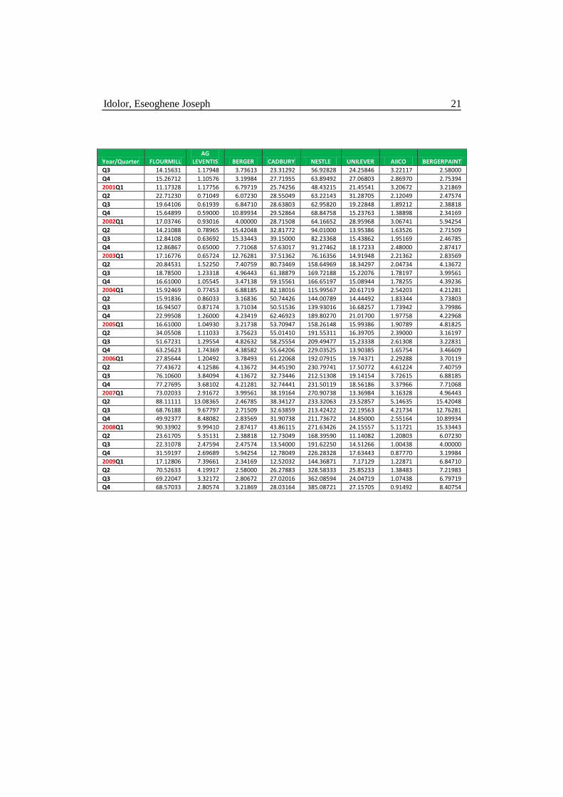
Year/Quarter FLOURMILL AG

LEVENTIS BERGER CADBURY NESTLE UNILEVER AIICO BERGERPAINT

Q3 14.15631 1.17948 3.73613 23.31292 56.92828 24.25846 3.22117 2.58000

Q4 15.26712 1.10576 3.19984 27.71955 63.89492 27.06803 2.86970 2.75394

2001Q1 11.17328 1.17756 6.79719 25.74256 48.43215 21.45541 3.20672 3.21869

Q2 22.71230 0.71049 6.07230 28.55049 63.22143 31.28705 2.12049 2.47574

Q3 19.64106 0.61939 6.84710 28.63803 62.95820 19.22848 1.89212 2.38818

Q4 15.64899 0.59000 10.89934 29.52864 68.84758 15.23763 1.38898 2.34169

2002Q1 17.03746 0.93016 4.00000 28.71508 64.16652 28.95968 3.06741 5.94254

Q2 14.21088 0.78965 15.42048 32.81772 94.01000 13.95386 1.63526 2.71509

Q3 12.84108 0.63692 15.33443 39.15000 82.23368 15.43862 1.95169 2.46785

Q4 12.86867 0.65000 7.71068 57.63017 91.27462 18.17233 2.48000 2.87417

2003Q1 17.16776 0.65724 12.76281 37.51362 76.16356 14.91948 2.21362 2.83569

Q2 20.84531 1.52250 7.40759 80.73469 158.64969 18.34297 2.04734 4.13672

Q3 18.78500 1.23318 4.96443 61.38879 169.72188 15.22076 1.78197 3.99561

Q4 16.61000 1.05545 3.47138 59.15561 166.65197 15.08944 1.78255 4.39236

2004Q1 15.92469 0.77453 6.88185 82.18016 115.99567 20.61719 2.54203 4.21281

Q2 15.91836 0.86033 3.16836 50.74426 144.00789 14.44492 1.83344 3.73803

Q3 16.94507 0.87174 3.71034 50.51536 139.93016 16.68257 1.73942 3.79986

Q4 22.99508 1.26000 4.23419 62.46923 189.80270 21.01700 1.97758 4.22968

2005Q1 16.61000 1.04930 3.21738 53.70947 158.26148 15.99386 1.90789 4.81825

Q2 34.05508 1.11033 3.75623 55.01410 191.55311 16.39705 2.39000 3.16197

Q3 51.67231 1.29554 4.82632 58.25554 209.49477 15.23338 2.61308 3.22831

Q4 63.25623 1.74369 4.38582 55.64206 229.03525 13.90385 1.65754 3.46609

2006Q1 27.85644 1.20492 3.78493 61.22068 192.07915 19.74371 2.29288 3.70119

Q2 77.43672 4.12586 4.13672 34.45190 230.79741 17.50772 4.61224 7.40759

Q3 76.10600 3.84094 4.13672 32.73446 212.51308 19.14154 3.72615 6.88185

Q4 77.27695 3.68102 4.21281 32.74441 231.50119 18.56186 3.37966 7.71068

2007Q1 73.02033 2.91672 3.99561 38.19164 270.90738 13.36984 3.16328 4.96443

Q2 88.11111 13.08365 2.46785 38.34127 233.32063 23.52857 5.14635 15.42048

Q3 68.76188 9.67797 2.71509 32.63859 213.42422 22.19563 4.21734 12.76281

Q4 49.92377 8.48082 2.83569 31.90738 211.73672 14.85000 2.55164 10.89934

2008Q1 90.33902 9.99410 2.87417 43.86115 271.63426 24.15557 5.11721 15.33443

Q2 23.61705 5.35131 2.38818 12.73049 168.39590 11.14082 1.20803 6.07230

Q3 22.31078 2.47594 2.47574 13.54000 191.62250 14.51266 1.00438 4.00000

Q4 31.59197 2.69689 5.94254 12.78049 226.28328 17.63443 0.87770 3.19984

2009Q1 17.12806 7.39661 2.34169 12.52032 144.36871 7.17129 1.22871 6.84710

Q2 70.52633 4.19917 2.58000 26.27883 328.58333 25.85233 1.38483 7.21983

Q3 69.22047 3.32172 2.80672 27.02016 362.08594 24.04719 1.07438 6.79719

Q4 68.57033 2.80574 3.21869 28.03164 385.08721 27.15705 0.91492 8.40754


Year/Quarter WAPCO OANDO UNIVERSITY

PRESS MOBIL TOTAL CAP VITA

FOAM NASCON ACADEMY GTBANK

Q3 23.61262 41.23569 3.48062 63.53615 66.89015 2.41723 4.15569 0.68692 0.87908 5.69017

Q4 24.34121 48.06030 3.20288 65.24909 67.68106 2.69212 4.46894 0.68697 0.79773 5.70000

2001Q1 20.80967 26.88000 3.55984 64.38311 64.10934 1.39098 3.97934 0.81213 0.92803 5.72591

Q2 20.65344 53.61426 2.86787 63.73230 62.24852 3.02475 3.73377 0.69000 0.80066 5.97455

Q3 18.54985 49.04182 2.21045 64.69030 66.09864 3.38682 3.94833 0.69000 0.78076 6.79571

Q4 14.93661 51.41271 2.01610 62.34966 67.05627 3.62966 4.73322 0.69000 0.54051 6.50639

2002Q1 19.49762 49.93333 3.46667 67.43349 66.54254 2.29348 4.01476 0.69000 0.82159 5.51338

Q2 15.03035 45.78070 1.64737 76.48544 75.78175 3.52000 3.92596 0.67368 0.91877 5.09780

Q3 15.20462 43.69354 1.48031 77.16077 93.75800 3.52400 3.94754 0.67615 0.92538 6.07603

Q4 17.66933 73.62250 1.37050 113.79850 151.92317 4.00950 4.13117 0.63000 1.49783 5.76509

2003Q1 16.01466 52.11052 1.73069 69.19052 71.54793 3.24207 5.27121 0.69000 0.56034 11.94000

Q2 17.65266 109.58484 1.71250 170.46531 219.22172 6.58094 3.97156 0.72000 3.07594 8.24067

Q3 13.57955 108.00000 1.65970 153.75106 189.82667 6.32091 3.28955 0.72000 2.79242 14.53859

Q4 1.49500 109.01667 1.27056 175.32296 189.79963 6.88444 3.36611 0.71259 1.93564 13.98469

2004Q1 19.72906 90.23000 1.63484 152.51906 245.38984 5.92656 4.30234 0.66469 2.55125 10.54103

Q2 10.35000 86.99033 1.29951 164.30705 170.10967 6.63525 3.17754 0.69000 1.85820 11.76273

Q3 10.46913 84.26544 1.56464 154.74623 192.49754 7.22261 3.99957 0.69000 1.72957 10.68579

Q4 17.47333 98.90233 1.40873 162.37127 190.37413 8.64000 4.48841 0.69000 1.50780 9.77492

2005Q1 10.86947 93.98316 1.66211 176.35105 177.19667 6.87263 3.35842 0.69000 1.91193 17.30823

Q2 22.79213 78.05656 2.56508 162.60770 187.67459 10.31197 3.47131 0.69000 1.26246 14.14836

Q3 47.55615 74.45000 2.79477 177.68046 196.93785 17.36108 4.05892 0.69000 1.23585 13.92303

Q4 56.56836 69.75569 3.20815 183.86000 190.31443 23.81581 4.12361 0.69000 1.35839 13.66763

2006Q1 18.15220 90.46153 1.71288 162.01881 187.51831 9.23780 5.07780 0.69000 1.47559 12.17833

Q2 67.06810 77.29293 7.03741 171.08534 172.82397 39.21310 6.20603 24.01810 4.82569 33.20190

Q3 25.61131 76.51031 8.17892 163.32062 161.37692 42.51385 7.64031 20.03415 5.90108 32.68462

Q4 66.68729 89.40051 7.11610 177.84339 166.52407 53.41000 8.26610 16.90559 5.44339 30.70576

2007Q1 67.75738 74.20689 3.20000 182.78590 187.03033 30.43754 4.22721 2.72541 2.17393 26.74885

Q2 57.31984 214.13714 11.58381 220.82603 237.94016 55.78794 11.52619 16.11698 11.74222 31.78286

Q3 43.22453 168.46484 8.30234 293.28078 238.42219 51.56766 9.93141 11.52281 7.30625 24.16016

Q4 29.45623 118.63311 6.95918 347.36721 232.64492 47.10508 7.20656 7.57721 5.62803 15.70131

2008Q1 70.43902 173.82820 12.49574 208.07820 209.71639 68.45230 11.39049 17.43541 7.43902 35.73049

Q2 20.97721 82.08082 6.11426 105.65115 150.81426 33.63820 4.42344 4.73049 5.75426 11.80836

Q3 29.95203 91.16391 6.68031 109.08813 146.56750 29.92547 4.06625 3.78906 4.75563 13.47328

Q4 29.98459 93.22869 4.84852 99.13705 154.32492 29.12918 5.04492 3.92148 4.87475 15.41590

2009Q1 16.66484 69.08984 4.39742 231.24129 148.73677 38.61435 4.31177 4.60339 5.41984 10.16952

Q2 41.24433 7.15667 7.15667 7.15667 220.12333 30.09550 6.57417 8.85650 6.11567 18.25433

Q3 38.74484 65.72719 7.15156 165.54641 248.25469 32.20266 6.33234 6.97484 16.10016 16.10016

Q4 40.34672 64.92967 6.39984 142.52230 225.02328 32.44459 6.14377 5.96918 3.86689 16.47574

Consumption Oriented Capital Asset Pricing Model and ...joc.hcc.edu.pk/articlepdf/Idolor Eseoghene...

Documents

Transcript of Consumption Oriented Capital Asset Pricing Model and ...joc.hcc.edu.pk/articlepdf/Idolor Eseoghene...