ISSN: 1439-2305

Number 285 – June 2016

CONSUMER INFORMATION IN A

MARKET FOR EXPERT SERVICES:

EXPERIMENTAL EVIDENCE

Tim Schneider

Lukas Meub

Kilian Bizer

Consumer Information in a Market for Expert Services:

Experimental Evidence

Tim Schneider∗†, Lukas Meub∗ and Kilian Bizer∗

Abstract

Markets for expert services are characterized by information asymmetries between

experts and consumers. We analyze the effects of consumer information, where consumers

suffer from either a minor or serious problem and only experts can infer the appropriate

treatment. Consumer information is a noisy signal that is informative about a consumer’s

problem severity. In a laboratory experiment, we show that consumers are generally

reluctant to accept expensive treatment recommendations, which is endorsed by good

signals and fundamentally changed by bad signals. Experts condition their cheating

on a consumer’s risk of suffering from a serious problem if they can observe consumer

information. Accordingly, experts and low-risk consumers benefit at the expense of more

frequently cheated high-risk consumers. Consumer information leads to more appropriate

treatments being carried out and thus superior overall welfare. In contrast to our theoretical

predictions, this effect does not depend on hiding consumer information for experts.

Keywords: consumer information; credence goods; experts; laboratory experiment

JEL: C70; C91; D82

∗Faculty of Economic Sciences, Chair of Economic Policy and SME Research, Goettingen University, Platzder Goettinger Sieben 3, 37073 Goettingen, Germany.

†Corresponding author, tim.schneider@wiwi.uni-goettingen.de, phone:+49-551-39-4438.

1 Introduction

In markets for expert services, consumers are incapable of determining adequate treatments

or services to solve their problem of a certain severity. Experts can perfectly infer both a

problem’s severity and the adequate service to solve the problem. Due to this ex ante information

asymmetry, consumers have to purchase not only an expert’s service but also information

given by the expert’s superior knowledge. In addition, ex post information asymmetries are

immanent as consumers are unable to verify the received service’s quality. Consequently, experts

have incentives to exploit their superior knowledge trough overcharging, undertreatment or

overtreatment (Dulleck and Kerschbamer 2006, 2009; Dulleck et al. 2011). Consumers anticipate

this exploitation and might thus refrain from contracting with experts. This leads to market

inefficiency or even market breakdown (Akerlof 1970). Examples of markets for expert services

are plentiful, with physicians, car mechanics, taxi drivers, home improvement contractors and

lawyers - to name just a few - providing services that match the outlined framework.

To protect consumers from being exploited while enhancing market efficiency, politics and

consumer groups have made consumer information campaigns their principle. This principle

is rooted in the idea that by equipping consumers with additional information, they are better

protected against bad deals while forcing experts to be more sincere in their recommendations

(Hadfield et al. 1998; Howells 2005). This approach has undoubtedly grown in importance and

tremendously expanded in scope over the last couple of years, complemented by the development

of various official websites, online initiatives aggregating and making available user content

(information) such as Wikipedia or communication through social media or message boards.

Consumers gather information about their likely problems and adequate services at minimal

cost, even for very specific issues (Murray 1991). However, the theoretical analysis by Hyndman

and Ozerturk (2011) challenges the folk wisdom assuming the general desirability of providing

more consumer information since experts might exploit this information to customize their

fraudulent service offers trough consumer discrimination.

Despite numerous studies on the effects of consumer knowledge about experts’ past behavior,

e.g. Akerlof (1970), Darby and Karni (1973) and Dulleck et al. (2011), those on the effects of

varying consumer information sets remain scarce. To our best knowledge, there is no controlled

laboratory study on the influence of varying consumer information on a market for expert

services. However, our theoretical predictions - which build on the work by Hyndman and

Ozerturk (2011) - show that this varying information and experts’ ability to observe it are

crucial in assessing the likely outcomes on markets for expert services.

Therefore, we design an experiment to evaluate the effects of additional consumer information

that alters the distinct properties of the information asymmetry between consumers and experts.

Consumers have either a serious or minor problem that needs to be solved by an expert

service. Before visiting an expert, consumers receive a noisy signal about their problem

severity. Liable experts observe the actual problem severity and recommend a verifiable cheap

or expensive treatment, whereby the cheap treatment only solves a minor problem and the

expensive treatment solves both. Accordingly, the only possibility for experts to cheat is

1

given by overtreatment.1 Consumers either accept the treatment recommendation, resulting

in the corresponding payoffs, or reject the treatment leaving the expert and consumer with an

outside option payment. Following a random matching protocol to avoid reputation building,

we introduce three treatments: (1) consumers receive an uninformative signal, (2) consumers

receive an informative signal observed by experts and (3) consumers receive an informative

signal hidden to experts. Our (3) treatment builds upon the finding of Hyndman and Ozerturk

(2011) who show that it might be optimal for consumers to hide their information to avoid being

cheated according to specific cheating tolerances.

While fraudulent behavior is evident across all treatment conditions, our results confirm the

findings of Lee and Soberon-Ferrer (1997), Fong (2003) as well as Balafoutas et al. (2013),

who show that experts tend to cheat consumers conditional on their identifiable characteristics,

i.e. they cheat high-risk consumers more frequently than neutral ones and low-risk consumers

the least. In contrast to our theoretical predictions, experts’ fraudulent behavior remains

unaffected from hiding consumer information. Consumers’ acceptance rates of expensive

treatments are quite low in the absence of consumer information, substantially increase with

bad signals and drop with good signals. Overall, more contracts are realized given additional

consumer information, whereby more problems are solved and aggregate welfare increases.

However, superior aggregate welfare benefits experts through more realized contracts and

low-risk consumers by being cheated less, while high-risk consumers are cheated more frequently

and become worse off.

Moreover, we argue that the design of consumers’ outside options has been somewhat

problematic in previous experimental studies. Outside option payments are realized if a

consumer rejects a treatment recommendation by the expert, which leaves the consumer’s

problem untreated. Thus far, consumers have received a payoff independent of their actual

problem severity. This design choice fails to meet real-life circumstances in many situations.

For instance, consider a patient suffering from either a minor (a cold) or a serious problem

(pneumonia). It is not to expect that the outside options when rejecting a treatment

recommendation are equivalent for both illness severities. Therefore, in our design, consumers

receive a lower payoff when suffering from an untreated serious problem than in case of an

untreated minor problem. This incentive structure has been described by Pitchek and Schotter

(1987).

Our findings add to the research on markets for expert services, whereby we deal with credence

goods. The term credence goods was introduced in the seminal paper by Darby and Karni (1973),

where ”generally speaking, credence goods have the characteristic that though consumers can

observe the utility they derive from the good ex post, they cannot judge whether the type or quality

they have received is the ex-ante needed one” (Dulleck et al. 2011, p.526). In the subsequent

strand of literature, it is generally assumed that consumers hold only vague information about

their problem that needs to be addressed by an expert (Angelova and Regner 2013; Emons

2001; Pesendorfer and Wolinsky 2003; Roe and Sheldon 2007). Homogeneous consumers are

only aware that they suffer from either a minor or a serious problem with common probabilities

1Liability precludes experts from undertreating consumers, while verifiability precludes overcharging.

2

(Bonroy et al. 2013; Dulleck and Kerschbamer 2006, 2009; Dulleck et al. 2011; Mimra et al.

2013, 2014; Wolinsky 1993).

Despite numerous investigations about varying mechanisms to overcome market inefficiencies in

expert markets,2 research about solving the dilemma through additional consumer information

is sparse. Darby and Karni (1973) show that experts’ optimal level of fraud is likely to decrease

with consumers’ knowledge. This corresponds to the folk wisdom that informed consumers are

less likely to be exploited as they more commonly tend to decline experts’ faulty advice. However,

Hyndman and Ozerturk (2011) show that in comparison to a setting with uninformed consumers,

experts’ cheating behavior depends on the specific signals: experts cheat consumers with a minor

problem most often when they have received a bad signal, whereas consumers receiving a good

signal are cheated the least. The authors conclude that more information does not necessarily

lead to less fraudulent expert behavior. In addition, Lee and Soberon-Ferrer (1997) as well as

Fong (2003) confirm that experts tend to cheat selectively based upon consumers’ identifiable

characteristics. Bonroy et al. (2013) show that in a market with homogeneous consumers who

are committed to a liable expert once she gives a recommendation, the higher the consumers’

risk aversion, the less likely experts are to invest in costly diagnosis. Fong (2003) - in accordance

with Pitchek and Schotter (1987) and Hyndman and Ozerturk (2011) - conclude that consumers

could be better off by withholding specific information, i.e. their expectation about having a

rather serious problem and being likely to require expensive treatment. Balafoutas et al. (2013)

identify consumers’ observable characteristics - e.g. income or city of origin - as being decisive for

experts’ tendency towards fraudulent behavior. In their field experiment, taxi drivers in Athens

were significantly more likely to overtreat and overcharge non-locals and high-income customers

when compared to locals and low-income customers. The authors conclude that these differences

in observable characteristics determine an expert’s perception of a consumer’s information set.

This perception translates to differences in a fraudulent act’s expected profit and ultimately in

different probabilities for consumers to be cheated. Overall, the effects of enhanced consumer

information depend on the distinct signals received and the experts’ ability to observe these

signals. Additional information does not imply superior market outcomes per se in the context

of expert services.

The remainder of this paper is structured as follows. Section two presents our theoretical

framework, before section three describes our experimental design and section four states our

hypothesis. Section five presents our results and finally section six concludes.

2 Theoretical Framework

Following the notation by Hyndman and Ozerturk (2011), we model a market for expert

services. Consumers suffer from either a minor or serious problem, denoted by ω ∈ {m, s}.

While they cannot observe their problem severity, the probability of suffering from a serious

2The effect of reputation and/or brand-naming goods (Akerlof 1970; Darby and Karni 1973; Grosskopf andSarin 2010; Dulleck et al. 2011; Mimra et al. 2013); the influence of competition (Dulleck et al. 2011; Mimra et al.2013); the possibility for second-opinion (Wolinsky 1993; Mimra et al. 2014).

3

problem is common knowledge and given by Pr(ω = s) = α ∈ (0, 1). Each consumer visits one

(monopolistic) expert, who can perfectly infer a consumer’s problem and recommends either

a cheap treatment at fixed price pm and cost cm or an expensive treatment at ps and cs,

where ps > pm and cs > cm. An expensive treatment solves both problem types, whereas a

cheap treatment solves only a minor problem. If a consumer accepts the recommendation, the

corresponding expert has to carry out the recommended treatment, i.e. treatments are assumed

to be verifiable. Given that we also assume liability, an accepted treatment recommendation

will always solve the consumer’s problem, which yields utility V . If a consumer rejects, both

the consumer and the expert receive an outside option σC and σE , respectively.

2.1 Payoffs

Payoff for experts

Given our assumptions of liability and verifiability, experts can exploit asymmetric information

by overtreatment only. Experts might recommend an expensive treatment despite a cheap

treatment being sufficient to solve a consumer’s problem. Experts might overtreat if the

mark-up for an expensive treatment exceeds a cheap treatment’s mark-up. We thus set

ps − cs = ys > ym = pm − cm with ym > 0 such that treating a consumer always yields positive

profits. We denote the expert cheating probability by β ∈ [0, 1]. In addition, we assume that

experts strictly prefer to treat consumers rather than falling back on the outside option, which

gives σE < ym.

Payoff for consumers

We assume that consumers suffer from a greater loss in utility given an untreated serious problem

rather than an untreated minor one, such that σcm > σcs. Consumers strictly prefer to be treated

with a suitable treatment rather than falling back on the outside option as V − ps > σcs and

V −pm > σcm. While consumers are unable to identify ex ante the severity of their problem, the

different outside options imply the ex post revelation of an untreated problem’s severity.3 Due to

the liability of experts, consumers will accept minor treatment recommendations with certainty.

Expensive treatment recommendations will only be accepted with a certain probability γ ∈ [0, 1].

Consumers are assumed to be better off when rejecting an expensive treatment given a minor

problem, which gives V − ps < σcm. Table 1 summarizes the payoff structure of the game.

2.2 Information

Before visiting an expert, consumers receive a signal on the severity of their problem. A

consumer’s type t ∈ T = {h, l, n} is referred to as high risk if he receives a bad signal, as

low risk if he receives a good signal and as neutral if he receives an uninformative signal. The

3We feel that these specific outside options are crucial to model actual conditions on expert markets.

Consumers can observe their utility from a treatment without knowing whether this solution was optimal.However, they are also able to observe their loss in utility for an untreated problem. Consider e.g. a personthat feels sick: while the person might be unsure about the severity of the illness ex-ante, they will definitelylearn about the severity of the illness when it remains untreated.

4

treatmentexpensive cheap rejected

problem serious (ω = s) V − ps, ps − cs -, - σcs, σEminor (ω = m) V − ps, ps − cs V − pm, pm − cm σcm, σE

Table 1: Summary of (consumer, expert) payoffs

probability of receiving a bad signal is given by q ∈ [0, 1]. Note that in our model a market

comprises either uninformed (t = n) or informed consumers (t = (l, h)) only. We exclude the

case where experts are confronted with informed and uninformed consumers at the same time.

Therefore, q always determines the proportion of high-risk consumers and (1−q) the proportion

of low-risk consumers in a market. Signal precision - denoted by φ - can be written as

φ ≡ Pr(t = h|ω = s) = Pr(t = l|ω = m) ∈

[

1

2, 1

)

(1)

We can derive the following posterior beliefs after consumers have learned about their type

αl ≡ Pr(s|l) =α(1− φ)

(1− α)φ+ α(1− φ)(2)

αh ≡ Pr(s|h) =αφ

αφ+ (1− α)(1− φ)(3)

αn ≡ Pr(s|n) = α. (4)

We exclude the trivial case where consumers always accept expensive treatment

recommendations by

V − ps < αtσcs + (1− αt)σcm, (5)

which gives

αt <V − ps − σcmσcs − σcm

. (6)

While experts can perfectly infer a consumer’s problem, expert behavior depends on their ability

to observe consumer signals. Therefore, we derive the equilibrium behavior conditional on

consumer types and experts’ ability to observe the underlying signals. The game trees in figure

1 illustrate our settings of the game, which we subsequently analyze in further detail.

5

(a) open consumer signal

(b) no consumer signal

(c) hidden consumer signal

Figure 1: Settings of the game

6

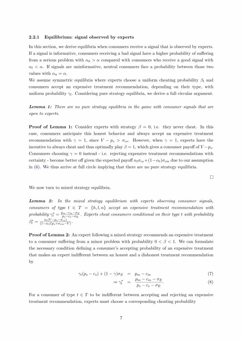
2.2.1 Equilibrium: signal observed by experts

In this section, we derive equilibria when consumers receive a signal that is observed by experts.

If a signal is informative, consumers receiving a bad signal have a higher probability of suffering

from a serious problem with αh > α compared with consumers who receive a good signal with

αl < α. If signals are uninformative, neutral consumers face a probability between those two

values with αn = α.

We assume symmetric equilibria where experts choose a uniform cheating probability βt and

consumers accept an expensive treatment recommendation, depending on their type, with

uniform probability γt. Considering pure strategy equilibria, we derive a full circular argument.

Lemma 1: There are no pure strategy equilibria in the game with consumer signals that are

open to experts.

Proof of Lemma 1: Consider experts with strategy β = 0, i.e. they never cheat. In this

case, consumers anticipate this honest behavior and always accept an expensive treatment

recommendation with γ = 1, since V − ps > σcs. However, when γ = 1, experts have the

incentive to always cheat and thus optimally play β = 1, which gives a consumer payoff of V −ps.

Consumers choosing γ = 0 instead - i.e. rejecting expensive treatment recommendations with

certainty - become better off given the expected payoff αtσcs+(1−αt)σcm due to our assumption

in (6). We thus arrive at full circle implying that there are no pure strategy equilibria.

�

We now turn to mixed strategy equilibria.

Lemma 2: In the mixed strategy equilibrium with experts observing consumer signals,

consumers of type t ∈ T = {h, l, n} accept an expensive treatment recommendation with

probability γ∗t = pm−cm−σE

ps−cs−σE. Experts cheat consumers conditional on their type t with probability

β∗t = αt(V−ps−σcs)

(1−αt)(ps+σcm−V ) .

Proof of Lemma 2: An expert following a mixed strategy recommends an expensive treatment

to a consumer suffering from a minor problem with probability 0 < β < 1. We can formulate

the necessary condition defining a consumer’s accepting probability of an expensive treatment

that makes an expert indifferent between an honest and a dishonest treatment recommendation

by

γt(ps − cs) + (1− γ)σE = pm − cm (7)

⇒ γ∗t =pm − cm − σEps − cs − σE

. (8)

For a consumer of type t ∈ T to be indifferent between accepting and rejecting an expensive

treatment recommendation, experts must choose a corresponding cheating probability

7

β∗t =

αt(σcs + ps − V )

(1− αt)(V − ps − σcm). (9)

If an expert cheats with a probability strictly greater [lower] than β∗t , a consumer of type t

always rejects [accepts] an expensive treatment recommendation. Moreover, β∗t increases with

a consumer’s belief about having a serious problem αt. Since experts observe consumer signals,

they are able to choose different strategies for each consumer type. Hence, in the mixed strategy

equilibrium, experts discriminate consumers according to their type-specific cheating tolerance.

High-risk consumers are cheated with a greater probability than neutral and low-risk consumers,

with the latter being cheated the least. Therefore, Hyndman and Ozerturk (2011) interpret β∗t

as the tolerance of consumers of type t towards being cheated. Since αh > αn > αl, we obtain

β∗h > β∗

n > β∗l . (10)

A consumer’s reaction function - conditional on an expert’s β - is given by

γt ∈

1 if β < β∗t

γ∗t if β = β∗t

0 if β > β∗t .

(11)

�

In the mixed strategy equilibrium, an expert’s expected profit is given by

πE(αt, γ∗t , β

∗t ) = αtγ

∗t (ps − cs) + αt(1− γ∗t )σE + (1− αt)β

∗t γ

∗t (ps − cs)

+ (1− αt)β∗t (1− γ∗t )σE + (1− αt)(1− β∗

t )(pm − cm), (12)

which can be rearranged by plugging in γ∗t = pm−cm−σE

ps−cs−σEto obtain

πopenE = pm − cm, (13)

where the superscript open refers to the case of an open signal observed by the expert. A

consumer’s expected profit is given by

πCt(αt, γ∗t , β

∗t ) = αtγ

∗t (V − ps) + αt(1− γ∗t )σCs + (1− αt)β

∗t γ

∗t (V − ps)

+ (1− αt)β∗t (1− γ∗t )σCm + (1− αt)(1− β∗

t )(V − pm). (14)

which can be rearranged by plugging in β∗t = αt(V−ps−σCs)

(1−αt)(ps+σCm−V ) to obtain

πopenCt (αt) = V − pm − αt

(σcs − σcm)(ps − pm)

V − ps − σcm. (15)

Since high-risk consumers are cheated more often, a consumer’s expected payoff decreases in the

risk αt of having a serious problem.

8

2.2.2 Equilibrium: signal not observed by experts

In this section, we assume that experts are no longer able to observe consumer signals.

Consequently, experts are incapable of discriminating consumers with respect to their

type-specific cheating tolerance. However, experts learn about the fractions of high- and

low-risk consumers in the market as they observe q, where (1− q) gives the fraction of low risk

consumers due to the absence of neutral-risk consumers.

Again, we arrive at a full circular argument in trying to identify pure strategy equilibria.

Lemma 3: There are no pure strategy equilibria in the game with consumer signals that are

hidden to experts.

Proof of Lemma 3: see proof of Lemma 1.

�

In the mixed strategy equilibrium, consumers’ acceptance strategy γ∗t - as derived in (7) - makes

the expert indifferent between cheating and being honest. However, since experts are no longer

able to discriminate with respect to consumer types, they have to choose a uniform strategy β

for all consumers.

If the expert sets β > β∗t [β < β∗

t ], consumers of type t will reject [accept] an expensive treatment

recommendation with certainty. Choosing β < β∗l [β > β∗

h] would make all consumers strictly

accept [reject] an expensive treatment recommendation, which contradicts equilibrium behavior

as described in the proof of Lemma 1.

This leaves the expert with two equilibria choices for β. By setting β = β∗h, the expert causes

all low-risk consumers to reject expensive treatment recommendations with certainty. This

would be optimal if the more frequent cheating of high-risk consumers (over-)compensates

the loss from low-risk consumers always rejecting expensive treatment recommendations. For

this consideration to hold true, an expert’s expected profit by setting β = β∗h needs to be

greater than her expected profit by choosing β = β∗l , i.e. πh

E(β∗h, γ

∗h, γl) > πl

E(β∗l , γh, γ

∗l ). If the

expert chooses β = β∗l instead, all high-risk consumers would accept an expensive treatment

recommendation with certainty and low risk-consumers, respectively, with γ∗l .

Lemma 4: If consumer information is hidden, experts always choose the low-risk consumer

equilibrium with β = β∗l = αl(σcs+ps−V )

(1−αl)(V−ps−σcm. In this scenario, high-risk consumers always accept

expensive treatment recommendations, i.e. γh = 1, and low-risk consumers play their mixed

strategy equilibrium, i.e. γ∗l = pm−cm−σe

ps−cs−σe.

Proof of Lemma 4: If experts choose β = β∗h = αh(σcs+ps−V )

(1−αh)(V−ps−σcm, all low-risk consumers reject

an expensive treatment recommendation all of the time, i.e. γl = 0. By contrast, all high-risk

consumers choose their mixed strategy equilibrium, i.e. γ∗h = pm−cm−σe

ps−cs−σe. In this scenario an

9

expert’s expected payoff is given by

πhE(αl, β

∗h) = q(pm − cm) + (1− q)[αlσe + (1− αl)βhσe + (1− αl)(1− βh)(pm − cm)], (16)

which gives

πhE(αl, β

∗h) = pm − cm − (1− q)[(pm − cm − σe)(αl + β∗

h − αlβ∗h)]. (17)

If experts choose instead β = β∗l = αl(σcs+ps−V )

(1−αl)(V−ps−σcmall high risk-consumers accept an expensive

treatment recommendation with certainty, i.e. γh = 1. By contrast, all low-risk consumers

choose their mixed strategy equilibrium, i.e. γ∗l = pm−cm−σe

ps−cs−σe. In this scenario, an expert’s

expected payoff is given by

πlE(αh, β

∗l ) = (1−q)(pm−cm)+q[αh(ps−cs)+(1−αh)βl(ps−cs)+(1−αh)(1−βl)(pm−cm)], (18)

which gives

πlE(αh, β

∗l ) = pm − cm + q[(ps − cs − pm + cm)(αh + β∗

l − αhβ∗l )]. (19)

Experts would choose the high-risk equilibrium if and only if πhE(αl, β

∗h) > πl

E(αh, β∗l ). However,

since we assume 0 < q < 1, πhE(αl, β

∗h) will never exceed πl

E(αh, β∗l ).

�

This property of our model stems from an unfavorable outside option for experts in case of

treatment rejections, making contracting - even by providing a cheap treatment - experts’

predominant objective if they are unable to observe consumer types. Consequently, experts

prefer the low-risk cheating equilibrium to maximize their number of realized contracts.

In this equilibrium, low-risk consumers’ expected profit is given by

πlCl(αl) = V − pm − αl

(σcs − σcm)(ps − pm)

V − ps − σcm. (20)

High-risk consumers’ expected profit is given by

πlCh(αh, β

∗l ) = V − pm − (αh + β∗

l − αhβ∗l )(ps − pm). (21)

2.3 Welfare

In the following, we analyze how consumer information affects welfare as measured by the

expected aggregate income and the distribution of income between consumers and experts.

10

2.4 Expert Welfare

No signal vs. open signal

If there is no consumer information - i.e. consumers receive an uninformative signal observed by

experts - all consumers are of the same type t = n and experts’ cheating probability becomes β∗n,

as described in (9). In case of informative signals observed by experts, consumers are cheated

with respect to their types and they choose their corresponding mixed strategy acceptance

probability γt = γ∗t , as shown in (7). The expected income of experts becomes equivalent for no

signal and open signal and is given by (13). We can write

∆πE = πnoSignalE (β∗

n)− πopenE (β∗

t ) = 0. (22)

Therefore, experts are indifferent between no consumer information at all and consumer

information that they can observe. Note that this result is independent of the actual share q of

high-risk consumers in the market.

Hidden signal vs. open signal

Given hidden signals, experts have to choose a uniform cheating probability βt = {β∗l , β

∗h}.

In this case, they cannot discriminate consumers along their cheating tolerance. According to

Lemma 4, experts always opt for β = β∗l and their expected payoff becomes (19). The expected

change in income in comparing an open and hidden signal can be written as

∆πlE = πl

E(β∗l )− πopen

E (β∗t ). (23)

By inserting and rearranging, we obtain

∆πlE = q[(ps − cs − pm + cm)(αh + β∗

l − αhβ∗l )] > 0. (24)

Since pm − cm < ps − cs, the expression is strictly positive and the expert is better off by not

observing consumer signals and being able to commit to the low-risk cheating equilibrium. In

addition, the proportion of high-risk consumers in the market determines the shift in income,

with a higher proportion the more intense it is.

2.5 Consumer Welfare

No signal vs. open signal

Consumers receiving either an uninformative signal or a signal observed by experts accept an

expensive treatment recommendation with probability γ∗t in the mixed strategy equilibrium,

which yields them an expected payoff as described in (15). As outlined above, consumer payoff

decreases with the probability of having a serious problem, i.e. αt. Therefore, the difference in

payoff depends on a consumer’s type and can be written as

11

∆πC = πnoSignalC (β∗

n)− πopenC (β∗

t ). (25)

which gives

∆πC = (αt − αn)(σcs − σcm)(ps − pm)

V − ps − σcm. (26)

As this ratio is strictly positive, high-risk consumers are worse off with an open signal since

αh > αn. By contrast, low-risk consumers are better off with an open signal since αl < αn.

Consequently, welfare is redistributed by consumer information from high- to low-risk consumers.

Hidden signal vs. open signal

Consumers receiving a signal that is not observed by experts are cheated with a uniform

probability βt = {β∗l , β

∗h} and react according to their reaction function described in

(11). By experts always setting β∗l , all high risk-consumers accept an expensive treatment

recommendation with certainty, i.e. γh = 1. Their expected income is given by (21). By

contrast, low-risk consumers accept an expensive treatment recommendation with γ∗l and their

expected payoff amounts to (20). Since low-risk consumers’ expected profit is equivalent for an

open and hidden signal, we can assess the difference in income by considering high-risk consumers

only. We arrive at

∆πlC = πl

Ch(γh, β∗l )− πopen

Ct=h(αh), (27)

which gives

∆πlC = q[(ps − pm)

(V − ps − σcs)(αl − αh)(1− αh)

(1− αl)(V − ps − σcm)] > 0. (28)

Since αl − αh < 0, as well as V − ps − σcm < 0, both the numerator and denominator are

negative. Consequently, the expression becomes strictly positive, implying that (high-risk)

consumers become better off by hiding consumer information.

2.6 Overall Welfare

Overall welfare is the aggregate of consumer and expert income. Both depend on the share of

high-risk consumers in the market and the availability of consumer information.

No signal vs. open signal

As previously mentioned, there are no differences for experts in terms of welfare when comparing

the scenarios of no signal and open signal. However, overall welfare depends on the share of

high-risk consumers in the market q, since consumers’ payoff decreases with the probability of

having a serious problem as shown in (15). We can write

∆π1 = πnoSignalC (β∗

n)− πopenC (β∗

t ), (29)

12

which gives

∆π1 =(σcs − σcm)(ps − pm)

V − ps − σcm[qαh + (1− q)αl − αn)]. (30)

With the fraction being strictly positive, whether market participants are better or worse off as

a whole, depends on the actual values of q, αh and αl.

Hidden signal vs. open signal

In case of hidden signals, experts choose the uniform cheating probability β = β∗l and consumers

react according to their reaction function given by (11). As previously mentioned, both

(high-risk) consumers and experts are better off in this scenario when consumer information

is hidden. This results from contracting generally being more favorable for experts. Experts

abstain from causing low-risk consumers to always reject expensive treatment recommendations

by choosing the low-risk cheating equilibrium and benefit from increased contracting rates. We

can write

∆π2 = πl(β∗l )− πopen(β∗

t ), (31)

which gives

∆π2 = πlE(β

∗l )− πopen

E (β∗t ) + πl

Ch(αh, β∗l )− πopen

Ct=h(αh) > 0. (32)

The expression is strictly positive, implying that overall welfare increases in this scenario by

hiding consumer information.

3 Experimental design

3.1 Overview of the game and parameterization

Our experimental design builds upon the theoretical framework and the assumptions described

above. Each session features one market for expert services comprising twelve subjects, similar

to Mimra et al. (2014). Subjects are randomly assigned to the role of an expert or consumer.

The roles remain constant throughout the eight periods of the game. Payoffs are denominated

in ECU, accumulated over periods and paid at the end of the experiment, where ECU 1 converts

to EUR 0.60.

Consumers suffer either from a serious or minor problem. The probability of having a serious

problem depends on a consumer’s type, i.e. αn = 0.5 without an informative signal and either

αl = 0.2 with a good signal or αh = 0.8 with a bad signal. Consumers are matched with one

expert who recommends an expensive or a cheap treatment. Experts learn about a consumer’s

problem at no cost. Experts can either recommend an expensive treatment which costs her

cs = 4 or cheap treatment which costs her cm = 3. Consumers can accept this treatment

recommendation and pay ps = 8 for an expensive treatment or pm = 5 for a cheap treatment.

An accepted expensive treatment solves both serious and minor problems, whereas a cheap

treatment only solves minor problems. If a consumer’s problem is solved, he earns V = 10. As

we assume liability, given a serious problem an expert is obliged to recommend an expensive

13

treatment. Accordingly, if a consumer accepts a treatment recommendation, his problem will

be solved with certainty. If a problem remains untreated - as a consumer rejects the expert’s

recommendation - the consumer as well as the expert earn an outside option. For a consumer,

the outside option depends on the severity of his problem, i.e. σcs = 1.6 in case of a serious

problem and σcm = 4 in case of a minor one. An expert’s outside option is independent of a

consumer’s problem and amounts to σE = 1.

According to the strategy method, experts recommend a treatment for each of the six consumers

in every period. Due to liability, experts only choose a treatment recommendation for the

hypothetical case that a consumer suffers from a minor problem. Experts observe the relevant

information for each consumer, i.e. a consumer’s likelihood of suffering from a minor or serious

problem, treatment prices and costs. Decisions are taken by checking radio buttons. However,

one expert is matched with only one consumer at the end of a period, and hence we assume

monopolistic experts. In order to avoid reputational concerns, the presentation of each consumer

- i.e. the position at which each consumer is displayed on the screen - is randomly determined

in each period (Dulleck et al. 2011).

The experts’ decision screen is shown in figure 2.

Figure 2: Expert decision screen

3.2 Treatment conditions

We implement three experimental treatment conditions that differ in terms of consumer

information and experts’ ability to observe this information.

noSignal: Consumers do not receive any informative signal about their likely problem and the

14

market comprises uninformed consumers (t = n) only. The probability of having a serious

problem is given by the ex-ante probability αn = 0.5.

openSignal: Consumers receive an informative signal before visiting an expert. Consumers are

of either high (t = h) or low risk (t = l). High-risk consumers face a αh = 0.8 chance

of suffering from a serious problem, whereas for low-risk consumers αl = 0.2. Experts

observe these signals.

hiddenSignal: Consumers receive an informative signal before visiting an expert. Consumers

are of either high (t = h) or low risk (t = l). High-risk consumers face a αh = 0.8 chance

of suffering from a serious problem, whereas for low-risk consumers αl = 0.2. Experts do

not observe these signals.

3.3 Course of the game

Each period of the game comprises six stages.

1. In openSignal and hiddenSignal each consumer is randomly selected to be of either high-

or low-risk type by receiving an informative signal that updates their probability to suffer

from a serious problem. In noSignal, all consumers receive the same uninformative signal.

2. Experts decide how to treat each of the six consumers given the hypothetical case that

they suffer from a minor problem. In openSignal, experts can identify a consumer’s

type, whereas they cannot observe the type in hiddenSignal. Experts can choose to

either overtreat a consumer by recommending an expensive treatment or act honestly

by recommending a cheap treatment.

3. Each consumer is randomly matched to one expert. Based on the type-specific

probabilities, it is randomly determined whether a consumer actually has a minor or

serious problem.

4. Consumers suffering from a serious problem are assigned an expensive treatment

recommendation in any case due to the liability assumption. Consumers suffering from a

minor problem are assigned the matched expert’s treatment recommendation.

5. Consumers observe the assigned treatment recommendation and decide to accept or reject.

6. If a consumer accepts, the recommendation with associated payoffs is implemented. If a

consumer rejects, both the expert and consumer are paid according to their outside option.

Each subject’s payoff from the current period and the cumulative payoff are displayed.

3.4 Procedure

For noSignal / openSignal / hiddenSignal, there were 8/8/7 sessions with 96/96/84 participants.

Experiments were conducted with a standard subject pool across disciplines in the Laboratory

of Behavioral Economics at the University of Goettingen; using ORSEE (Greiner 2004) and

15

z-Tree (Fischbacher 2007). The sessions lasted about 40 minutes, whereby subjects earned EUR

11.50 on average.

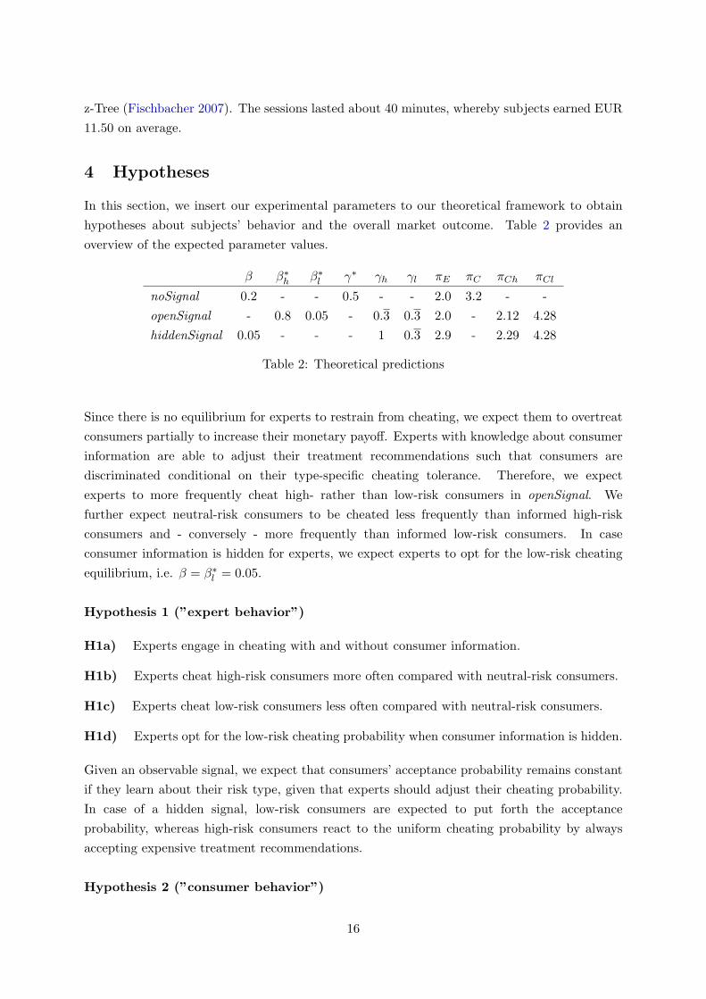
4 Hypotheses

In this section, we insert our experimental parameters to our theoretical framework to obtain

hypotheses about subjects’ behavior and the overall market outcome. Table 2 provides an

overview of the expected parameter values.

β β∗h β∗

l γ∗ γh γl πE πC πCh πCl

noSignal 0.2 - - 0.5 - - 2.0 3.2 - -

openSignal - 0.8 0.05 - 0.3 0.3 2.0 - 2.12 4.28

hiddenSignal 0.05 - - - 1 0.3 2.9 - 2.29 4.28

Table 2: Theoretical predictions

Since there is no equilibrium for experts to restrain from cheating, we expect them to overtreat

consumers partially to increase their monetary payoff. Experts with knowledge about consumer

information are able to adjust their treatment recommendations such that consumers are

discriminated conditional on their type-specific cheating tolerance. Therefore, we expect

experts to more frequently cheat high- rather than low-risk consumers in openSignal. We

further expect neutral-risk consumers to be cheated less frequently than informed high-risk

consumers and - conversely - more frequently than informed low-risk consumers. In case

consumer information is hidden for experts, we expect experts to opt for the low-risk cheating

equilibrium, i.e. β = β∗l = 0.05.

Hypothesis 1 (”expert behavior”)

H1a) Experts engage in cheating with and without consumer information.

H1b) Experts cheat high-risk consumers more often compared with neutral-risk consumers.

H1c) Experts cheat low-risk consumers less often compared with neutral-risk consumers.

H1d) Experts opt for the low-risk cheating probability when consumer information is hidden.

Given an observable signal, we expect that consumers’ acceptance probability remains constant

if they learn about their risk type, given that experts should adjust their cheating probability.

In case of a hidden signal, low-risk consumers are expected to put forth the acceptance

probability, whereas high-risk consumers react to the uniform cheating probability by always

accepting expensive treatment recommendations.

Hypothesis 2 (”consumer behavior”)

16

H2a) Consumers accept expensive treatment recommendations with the same probability

when there is no consumer information and with an open signal.

H2b) Consumers receiving an open signal show an acceptance probability for expensive

treatment recommendation independent of their specific risk type.

H2c) High-risk consumers accept all expensive treatment recommendations when consumer

information is hidden, whereas low-risk consumers show the same probability to accept

without or with observable consumer information.

Since there is an equal proportion of high- and low-risk consumers in the market with q = 0.5

and corresponding symmetric probabilities of serious problems of P (ω = s|t = h) = αh = 0.8

as 1 − αh = αl = 0.2, there should be no difference in aggregate income due to open signals

when compared to no consumer information. However, we expect a redistribution of income

from high- to low-risk consumers. According to our theoretical predictions, in case the signal

becomes hidden, we expect an increase in experts’ and high-risk consumers’ welfare. Since

low-risk consumers’ welfare should remain constant, we expect an overall increase in welfare

when consumer signals are hidden.

Hypothesis 3 (”welfare”)

H3a) Overall welfare remains constant if observable consumer information is introduced.

H3b) If consumer information is hidden to experts, overall welfare increases due to more

contracts between high-risk consumers and experts.

H3c) High-risk consumers benefit from introducing observable information, while low-risk

consumers generate less income.

5 Results

We analyze our experimental data according to the structure of our hypotheses: first, we

investigate expert cheating; second, we investigate consumer acceptance; and third, we reach

an overall conclusion by deriving aggregate income conditional on the availability of consumer

information. Unless mentioned otherwise, all tests are carried out treating one market as one

observation only.

5.1 Expert behavior

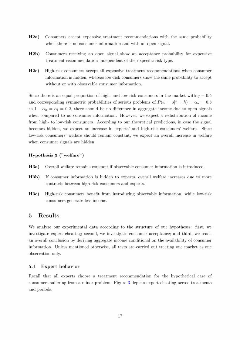
Recall that all experts choose a treatment recommendation for the hypothetical case of

consumers suffering from a minor problem. Figure 3 depicts expert cheating across treatments

and periods.

17

0

.1

.2

.3

.4

.5

.6

.7

.8

.9

1

share

dis

honest re

com

mendations

1 2 3 4 5 6 7 8

period

noSignal hiddenSignal

openSignal openSignal_good openSignal_bad

Figure 3: Experts’ dishonest treatment recommendations

For all treatments, there is a considerable fraction of dishonest treatment recommendations,

which is rather constant over time. In noSignal/openSignal/hiddenSignal the average share of

dishonest recommendations amounts to 0.59/0.56/0.57, which gives strong evidence in support

of H1a. On average, experts tend to cheat much more frequently than predicted by theory

when there is no consumer information (0.59 > βn = 0.2) or hidden consumer information

(0.57 > β∗l = 0.05). We further hypothesized (H1b/H1c) that consumers in open signal will

be cheated according to their cheating tolerance, which holds true as the fraction of dishonest

recommendation in case of bad signals amounts to 0.8 (= β∗h) and only 0.31(> β∗

l = .05) in

case of good signals. Both are significantly different from the fraction cheated when there is

no additional consumer information (Wilcoxon-Rank-Sum-test: for high risk z = −2.100 and

p = .0357; for low risk z = 3.046 and p = .0023) and when there is hidden consumer information

(Wilcoxon-Rank-Sum-test: for high risk z = 2.083 and p = .0372; for low risk z = −2.893

and p = .0038). However, there is no difference in cheating behavior between noSignal and

hiddenSignal, which contradicts H1d (WRS test: z = .753 and p = .4515).

To assess expert behavior in further detail, we address cheating at the individual level in figure

4.

18

0.2

.4.6

.81

share

dis

honest re

com

mendations

noSignal openSignal_good openSignal_bad hiddenSignal

Figure 4: Distribution of experts’ dishonest treatment recommendations

It becomes evident that cheating behavior is quite homogeneous. The fraction of approximately

60% dishonest treatment recommendations in noSignal and hiddenSignal do not stem from

experts either cheating all the time or never cheating; rather,they apply a mixed strategy of

cheating with a certain probability. There are 14.58/2.08/7.14% (4.17/4.17/7.14%) of experts

who always (never) overtreat their consumers.

Result 1: Experts tend to cheat much more often than suggested by theory when there

is no additional consumer information. Experts adjust their treatment recommendations to

account for differences in consumers’ cheating tolerance. Experts do not adjust their treatment

recommendations in terms of whether there is no consumer information or hidden consumer

information.

5.2 Consumer behavior

Figure 5 depicts the fraction of realized contracts, the equivalent to accepted recommendations

subject to experts’ treatment recommendations.

19

0

.1

.2

.3

.4

.5

.6

.7

.8

.9

1

1 2 3 4 5 6 7 8 1 2 3 4 5 6 7 8

cheap expensive

noSignal openSignal hiddenSignal

accepta

nce r

ate

period

Figure 5: Consumer acceptance conditional on treatment recommendations

The acceptance rate in case of cheap treatment recommendations is close to - but not

perfectly - 1 and there is neither a trend over time nor a substantial difference across

treatments (Kruskal-Wallis test: χ2 = 3.113 and p = .2109). For expensive treatment

recommendations, in noSignal there are significantly more rejections compared to openSignal

and hiddenSignal (Kruskal-Wallis test: χ2 = 14.048 and p = .009), which contradicts H2a.

Without additional consumer information, consumers are more reluctant to accept expensive

treatment recommendations than suggested by theory (.29 < γ∗ = .5). Therefore, consumers

with additional information tend to accept expensive treatment recommendations significantly

more often, which can be analyzed in further depth by differentiating acceptance with respect

to the signals received as shown in figure 6.

20

0

.1

.2

.3

.4

.5

.6

.7

.8

.9

1

1 2 3 4 5 6 7 8 1 2 3 4 5 6 7 8 1 2 3 4 5 6 7 8 1 2 3 4 5 6 7 8

cheap, good cheap, bad expensive, good expensive, bad

openSignal hiddenSignal

accepta

nce r

ate

period

Figure 6: Consumer acceptance conditional on treatment recommendations and signals

Optimal behavior suggests that cheap treatment recommendation should always be accepted.

As expected, we find no specific pattern with respect to good or bad signals. However, it has to

be considered that there are very few observations for consumers who received a cheap treatment

recommendation and a bad signal, which explains the peaks in graphs.4

In case of expensive treatment recommendations, there is an evident difference with respect

to consumers’ received signals. Recall that we expected that the probability of accepting an

expensive treatment remains constant over treatments with γl/h = 0.3, except for high-risk

consumers in hiddenSignal who should always accept an expensive treatment recommendation

(cp. table 2).

If consumers received a bad signal, they are substantially more willing to accept a serious

treatment recommendation (Wilcoxon matched-pairs signed-ranks test: for openSignal z =

−2.521 and p = .0117; for hiddenSignal z = −2.366 and p = .0180), which detrimentally

contradicts H2b, where we hypothesized that the acceptance probability is independent of the

specific risk type when there is an open signal. However, there are no differences due to signals

being open or hidden to the expert (WRS test: for good signal z = 1.158 and p = .2467; for bad

signals z = 0.926 and p = .3545). This has to be interpreted as mixed evidence with respect to

H2c.

Result 2: Consumers tend to frequently reject expensive treatment recommendations if they

do not receive additional information. Good signals are associated with very low levels of

acceptance, while bad signals are associated with very high levels of acceptance. Whether the

signal is open or hidden to the expert has no influence on this basic pattern.

4In openSignal this pattern occurred only eight times, in hiddenSignal ten times.

21

5.3 Welfare

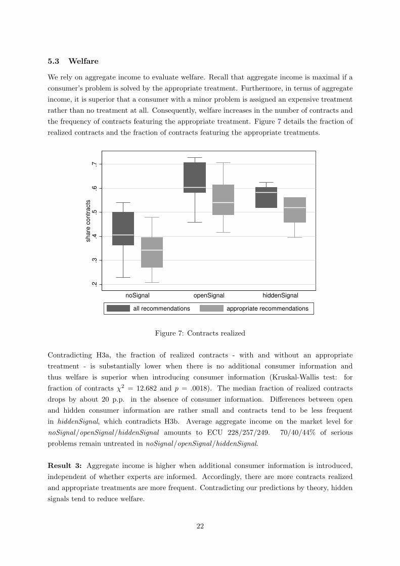
We rely on aggregate income to evaluate welfare. Recall that aggregate income is maximal if a

consumer’s problem is solved by the appropriate treatment. Furthermore, in terms of aggregate

income, it is superior that a consumer with a minor problem is assigned an expensive treatment

rather than no treatment at all. Consequently, welfare increases in the number of contracts and

the frequency of contracts featuring the appropriate treatment. Figure 7 details the fraction of

realized contracts and the fraction of contracts featuring the appropriate treatments.

.2.3

.4.5

.6.7

share

contr

acts

noSignal openSignal hiddenSignal

all recommendations appropriate recommendations

Figure 7: Contracts realized

Contradicting H3a, the fraction of realized contracts - with and without an appropriate

treatment - is substantially lower when there is no additional consumer information and

thus welfare is superior when introducing consumer information (Kruskal-Wallis test: for

fraction of contracts χ2 = 12.682 and p = .0018). The median fraction of realized contracts

drops by about 20 p.p. in the absence of consumer information. Differences between open

and hidden consumer information are rather small and contracts tend to be less frequent

in hiddenSignal, which contradicts H3b. Average aggregate income on the market level for

noSignal/openSignal/hiddenSignal amounts to ECU 228/257/249. 70/40/44% of serious

problems remain untreated in noSignal/openSignal/hiddenSignal.

Result 3: Aggregate income is higher when additional consumer information is introduced,

independent of whether experts are informed. Accordingly, there are more contracts realized

and appropriate treatments are more frequent. Contradicting our predictions by theory, hidden

signals tend to reduce welfare.

22

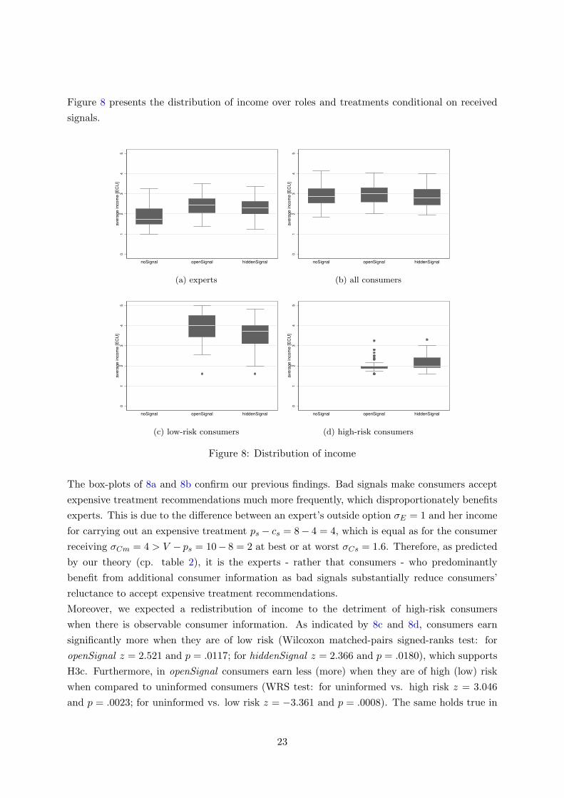
Figure 8 presents the distribution of income over roles and treatments conditional on received

signals.0

12

34

5

avera

ge incom

e [E

CU

]

noSignal openSignal hiddenSignal

(a) experts

01

23

45

avera

ge incom

e [E

CU

]

noSignal openSignal hiddenSignal

(b) all consumers

01

23

45

avera

ge incom

e [E

CU

]

noSignal openSignal hiddenSignal

(c) low-risk consumers

01

23

45

avera

ge incom

e [E

CU

]

noSignal openSignal hiddenSignal

(d) high-risk consumers

Figure 8: Distribution of income

The box-plots of 8a and 8b confirm our previous findings. Bad signals make consumers accept

expensive treatment recommendations much more frequently, which disproportionately benefits

experts. This is due to the difference between an expert’s outside option σE = 1 and her income

for carrying out an expensive treatment ps − cs = 8− 4 = 4, which is equal as for the consumer

receiving σCm = 4 > V − ps = 10− 8 = 2 at best or at worst σCs = 1.6. Therefore, as predicted

by our theory (cp. table 2), it is the experts - rather that consumers - who predominantly

benefit from additional consumer information as bad signals substantially reduce consumers’

reluctance to accept expensive treatment recommendations.

Moreover, we expected a redistribution of income to the detriment of high-risk consumers

when there is observable consumer information. As indicated by 8c and 8d, consumers earn

significantly more when they are of low risk (Wilcoxon matched-pairs signed-ranks test: for

openSignal z = 2.521 and p = .0117; for hiddenSignal z = 2.366 and p = .0180), which supports

H3c. Furthermore, in openSignal consumers earn less (more) when they are of high (low) risk

when compared to uninformed consumers (WRS test: for uninformed vs. high risk z = 3.046

and p = .0023; for uninformed vs. low risk z = −3.361 and p = .0008). The same holds true in

23

hiddenSignal (WRS test: for uninformed vs. high risk z = 1.967 and p = .0491; for uninformed

vs. low risk z = −3.240 and p = .0012).

Result 4: Experts benefit from introducing consumer information due to the substantial

reduction in consumers’ reluctance to accept expensive treatment recommendation when

receiving bad signals. For both open and hidden signals, low-risk consumers benefit from

additional consumer information, while high-risk consumers are worse off.

6 Conclusion

In the literature, there is plenty of research about markets for expert services, in which

ex-ante consumer information has not gained much attention. However, providing additional

consumer information is among the most prominent proposals to overcome the inefficiencies

due to asymmetric information. Therefore, we have investigated how consumers receiving an

informative yet noisy signal before visiting an expert influences experts’ cheating behavior,

consumers’ acceptance probabilities and overall welfare in a market for expert services. In our

theoretical model, we introduced three different treatments in which consumers receive either

(1) an uninformative signal, (2) an informative signal observed by experts or (3) an informative

signal hidden to experts. We built closely on the incentive structure by Pitchek and Schotter

(1987), i.e. there is a difference in consumer welfare conditional on the severity of an untreated

problem. Our model enables us to derive behavioral hypotheses on the effects of additional

consumer information, which we tested experimentally.

We find that experts’ likelihood of fraudulent behavior - i.e. recommending an expensive

treatment when a cheap one would be sufficient to solve a consumer’s problem - is influenced

by ex-ante consumer information observed by experts. Our results confirm the findings of Lee

and Soberon-Ferrer (1997), Fong (2003) as well as Balafoutas et al. (2013) that experts tend

to cheat consumers conditional on their identifiable characteristics, which is given by the risk

type in our setting determined by received signals. Our data shows that experts cheat high-risk

consumers significantly more often than low-risk consumers, which supports the hypothesis by

Hyndman and Ozerturk (2011) that hiding bad signals might be beneficial to consumers. Our

results thus indicate that - in contrast to common sense - uninformed consumers are not the

most likely victims of fraudulent behavior; rather, it is the informed high-risk type. In contrast

to our theoretical predictions, we do not find any influence on experts’ fraudulent behavior by

hiding consumers’ signals compared to the case of no ex-ante consumer information.

Moreover, our results show a significant influence of consumers’ information on their acceptance

probability for expensive treatments. Without additional information, consumers show

substantially lower rates of acceptance than suggested by theory. This might be due to consumers

hoping for a minor problem, in which case the outside option doubles their income in comparison

to accepting an expensive treatment. In the worst case, they fall back on the outside option

and suffer from a serious problem, which only reduces their income by 20%. Accordingly,

the risk in monetary terms of an untreated serious problem compared to a treated one was

24

quite small. Based on this consideration, it is quite surprising that consumers substantially

change their behavior and show very high acceptance probabilities when receiving bad signals.

Since consumers condition their behavior on the received signals, more serious problems are

treated appropriately with informative signals. However, there is no evidence that consumers

account for experts’ ability to observe their signals as they behave similarly in terms of accepting

probabilities in case of hidden and open signals.

Aggregate income increases when there is additional consumer information. This stems from

consumers’ tendency to reject expensive treatment recommendation if they do not distinctively

receive a bad signal. In case of open signals, low cheating probabilities associated with good

signals meet low acceptance rates of expensive treatments, whereas bad signals are associated

with high cheating probabilities and high acceptance rates. This results in more realized

contracts and more consumer problems are solved appropriately. In case of hidden signals,

experts tend to cheat as if there was no consumer information, while consumers with bad signals

show higher acceptance rates of expensive treatments. Again, there are more contracts realized

and especially more serious problems solved.

In sum, markets for expert services generate superior levels of overall welfare when there is

additional ex-ante consumer information. This is driven by experts benefiting from more

frequently accepted expensive treatment recommendations implying more realized contracts and

less outside option payments. Whether consumers benefit or not crucially depends on risk types,

where low-risk consumers are better off and high-risk consumers are worse off when introducing

additional consumer information.

25

Acknowledgement

We are grateful to Rudolf Kerschbamer, Christian Waibel, Till Proeger and various seminar

participants for useful comments and suggestions. Financial support for conducting the

laboratory experiments from the German Federal Ministry of Education and Research is

gratefully acknowledged (Grant number 03EK3517).

26

References

Akerlof, George A. The market for lemons: Quality uncertainty and the market mechanism.

The Quarterly Journal of Economics, 84(3):488–500, 1970.

Angelova, Vera and Tobias Regner. Do voluntary payments to advisors improve the quality

of financial advice? an experimental deception game. Journal of Economic Behavior &

Organization, 93(100):205–218, 2013.

Balafoutas, Loukas, Adrian Beck, Rudolf Kerschbamer, and Matthias Sutter. What drives taxi

drivers? a field experiment on fraud in a market for credence goods. Review of Economic

Studies, 80(3):867–891, 2013.

Bonroy, Olivier, Stephane Lemarie, and Jean-Philippe Tropeano. Credence goods, experts and

risk aversion. Economics Letters, 120(3):464–467, 2013.

Darby, Michael R. and Edi Karni. Free competition and the optimal amount of fraud. Journal

of Law and Economics, 16(1):67–88, 1973.

Dulleck, Uwe and Rudolf Kerschbamer. On doctors, mechanics, and computer specialists: The

economics of credence goods. Journal of Economic Literature, 44(1):5–42, 2006.

Dulleck, Uwe and Rudolf Kerschbamer. Experts vs. discounters: Consumer free-riding and

experts withholding advice in markets for credence goods. International Journal of Industrial

Organization, 27(1):15–23, 2009.

Dulleck, Uwe, Rudolf Kerschbamer, and Matthias Sutter. The economics of credence goods:

An experiment on the role of liability, verifiability, reputation, and competition. American

Economic Review, 101(2):526–555, 2011.

Emons, Winand. Credence goods monopolists. International Journal of Industrial Organization,

19(3-4):375–389, 2001.

Fischbacher, Urs. z-tree: Zurich toolbox for ready-made economic experiments. Experimental

Economics, 10(2):171–178, 2007.

Fong, Yuk-fai. When do experts cheat and whom do they target? The RAND Journal of

Economics, 36(1):113–130, 2003.

Greiner, Ben. An online recruitment system for economic experiments. GWDG Berichte, 63:

79–93, 2004.

Grosskopf, Brit and Rajiv Sarin. Is reputation good or bad? an experiment. American Economic

Review, 100(5):2187–2204, 2010.

Hadfield, Gillian K., Robert Howse, and Michael J. Trebilcock. Information-based principles for

rethinking consumer protection policy. Journal of Consumer Policy, 21(2):131–169, 1998.

27

Howells, Geraint. The potential and limits of consumer empowerment by information. Journal

of Law and Society, 32(3):349–370, 2005.

Hyndman, Kyle and Saltuk Ozerturk. Consumer information in a market for expert services.

Journal of Economic Behavior & Organization, 80(3):628–640, 2011.

Lee, Jinkook and Horacio Soberon-Ferrer. Consumer vulnerability to fraud: Influencing factors.

The Journal of Consumer Affairs, 31(1):70–89, 1997.

Mimra, W., A. Rasch, and C. Waibel. Price competition and reputation in credence goods

markets: Experimental evidence: Working Paper 13/176 March 2013. Zurich, 2013.

Mimra, Wanda, Alexander Rasch, and Christian Waibel. Second Opinions in Markets for Expert

Services: Experimental Evidence: Working Paper 14/192. Zurich, 2014.

Murray, Keith B. A test of services marketing theory: Consumer information acquisition

activities. Journal of Marketing, 55(1):10–25, 1991.

Pesendorfer, Wolfgang and Asher Wolinsky. Second opinions and price competition: Inefficiency

in the market for expert advice. Review of Economic Studies, 70:417–437, 2003.

Pitchek, Carolyn and Andrew Schotter. Honesty in a model of strategic information

transmission. The American Economic Review, 77(5):1032–1036, 1987.

Roe, B. and I. Sheldon. Credence good labeling: The efficiency and distributional implications

of several policy approaches. American Journal of Agricultural Economics, 89(4):1020–1033,

2007.

Wolinsky, Asher. Competition in a market for informed experts’ services. The RAND Journal

of Economics, 24(3):380, 1993.

28

Appendix A - Instructions

General Information about the Experiment

There are twelve participants and eight periods in the experiment. The course of a period is the

same for all periods. In each period, new pairs of two participants will be matched randomly.

Each pair comprises exactly one player with role A and one player with role B. In general, the

experiment is about player B having a problem in each period, which can be solved by an action

of player A. In the beginning of the experiment, it will be randomly determined whether you

are playing as player A or player B: therefore, half of all participants will be playing as player A

and the other half as player B. The roles remain fixed throughout the course of the experiment.

Your profit in this experiment is calculated in credits with 1 credit = 0.60 Euro. At the end

of the experiment, your income will be converted from credits into Euros and paid to you. Your

final payoff depends on your own and other participants’ decisions. At the end of each period

you will see your own payoff from this period, as well as how much you earned over all periods

up to this point.

In every period player B has exactly one problem: either problem 1 or problem 2. The problem

will again be determined randomly in each period for each player B, independently and with

a fixed probability. [T1: The probability of player B having problem 1 is 50%. Consequently,

the probability of player B having problem 2 is also 50%.] [T2,T3: The probability of player B

having either problem 1 or problem 2 depends on his type: either type 1 or type 2.] Player B’s

type is again randomly determined in each round. The relations are displayed in the following

table:

Player B with... Probability of having Probability of having

Problem 1 Problem 2

Type 1 80 % 20 %

Type 2 20 % 80 %

The table can be read in the following way:

• If you are a player B type 1, your probability of having problem 1 is 80% and the probability

of having problem 2 is 20%.

• If you are a player B type 2, your probability of having problem 1 is 20% and the probability

of having problem 2 is 80%.]

As a player B you will never be informed which problem you actually have. [T2,T3:

You are merely informed about your probability of having either problem 1 or problem 2.]

29

General Course of the Experiment

The course for each of the eight periods is identical and summarized in the following:

1. Player A decides which actions she wants to take.

2. Pairs are matched randomly and each player B’s actual problem is determined.

3. Player B decides whether he wants to accept player A’s proposed action.

4. Each player is informed about her/his payoff.

In the following, each stage is explained in detail. Additionally, player A’s and player B’s

payoffs are summarized on the last page of the instructions.

1. Player A’s Action

Player A’s task is to solve player B’s problem through her action. In each round, she can choose

between two distinct actions: action 1 or action 2. The selectable actions for player A depend

on player B’s actual problem in each round:

• If player B has problem 1, player A can choose both action 1 or action 2. Both actions

solve the problem but lead to different costs and earnings for player A and player B.

• If player B has problem 2, player A has to solve this by choosing action 2.

Each action leads to different earnings for player A, which have to be paid by player B (player

B’s payoff will be described later):

• Action 1: Player B pays 5 credits to player A.

• Action 2: Player B pays 8 credits to player A.

In addition, each action causes different costs for player A:

• Action 1 induces costs of 3 credits.

• Action 2 induces costs of 4 credits.

In the beginning of each round, player A decides for each of the six players B, which action she

wants to carry out for each of them. At this time, player A does not know about the player B

with which she will be matched in this round. Consequently, player A decides in advance

how she wants to behave towards each player B in case she will be matched to him.

The position where all player Bs are represented on the screen will be randomly determined in

each round.

For illustrative purposes, player A’s decision screen is presented below:

30

T1:

T2:

31

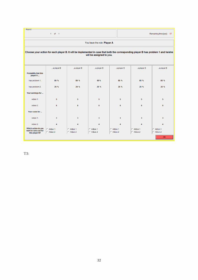
T3:

32

[T1,T2: Player A can observe each player B’s probability of having either problem 1 or problem

2.] [T3: Player A cannot observe players B’s probabilities of having either problem 1 or problem

2. Therefore, player A remains uninformed about whether a specific player B is either type 1

or type 2. However, she knows that a player B’s probability of being either type 1 or type 2

is 50%.] Moreover, player A’s costs and earnings for action 1 and action 2 are shown on the

screen. At the bottom of the screen, player A has to choose which action she wants to carry out

for each player B. For each player B a decision has to be made.

Note that in case player B has problem 2, player A has to carry out action 2. If the player B who

is actually matched to her has problem 2, action 2 will be assigned automatically to this player

A. Therefore, the decision made by player A is only implemented if the matched

player B has problem 1!

2. Matching and Determining Player B’s Problem

After all players A chose their actions for a period, each player B is randomly matched with one

player A. The random matching is carried out in each round.

Subsequently, for each player B it is determined - according to his type and the corresponding

probabilities - whether he has problem 1 or problem 2.

33

• If a player B has problem 1, the matched player A’s chosen action is presented to him.

This can be either action 1 or action 2.

• If a player B has problem 2, action 2 is presented to him automatically, since player

A has no choice in this case than to carry out action 2.

Since player B does learn about his actual problem, he cannot infer - in case action 2 was

chosen for him - whether player A chose action 2 or if it was assigned automatically.

3. Player B’s Action

Player B knows whether action 1 or action 2 was chosen for him and learned about the underlying

probabilities of having either problem 1 or problem 2 in this period. However, he is not informed

about his actual problem. Player B now decides whether to accept or reject the chosen action.

• If player B accepts the action, it will be implemented. Player B receives a payment

of 10 credits. These 10 credits are reduced by the amount that player B has to pay to

his matched player A for her action. Player A’s earnings are reduced by the cost of the

action.

• If player B rejects the action, both players receive an outside payment. Player A’s

outside payment amounts to 1 credit. The amount of player B’s outside payment depends

on whether he had problem 1 (= 4 credits) or problem 2 (= 1.6 credits) in this period.

For illustrative purposes, player B’s decision screen is presented below:

T1:

34

T2:

35

T3:

A period ends after player B’s decision. At the end of each round...

• each player A is informed which actual problem her matched player B had, which

action she took accordingly and whether this player B accepted or rejected this action.

• each player B is informed which action was chosen for him and whether he accepted

or rejected the action, but not which problem he actually had.

At the end of each period, player A and player B are informed about their payoffs from this

period and how much they have earned over all periods up to this point.

Payoff Summary

The payoffs for player A and player B depend on their choices within the matched pair.

Player A’s payoff for each period:

• If the matched player B accepts the action:

Payoff = earnings from action - costs from action

• If the matched player B rejects the action:

Payoff = outside payment = 1 credit

Player A’s payoffs are summarized in the following table:

36

Accepted Action 1 Accepted Action 2 Rejection

Player B has 2 credits 4 credits 1 credit

Problem 1

Player B has - 4 credits 1 credit

Problem 2

Player B’s payoff for each period:

• If the action of the matched player A is accepted:

Payoff = 10 credits - player A’s earnings for the action

• If the action of the matched player A is rejected and player B had problem 1:

Payoff = outside payment = 4 credit

• If the action of the matched player A is rejected and player B had problem 2:

Payoff = outside payment = 1.6 credits

Player B’s payoffs are summarized in the following table:

Accepted Action 1 Accepted Action 2 Rejection

Player B has 5 credits 2 credits 4 credit

Problem 1

Player B has - 2 credits 1.6 credit

Problem 2

The payoffs from each period will be summed up and paid out at the end of the experiment.

37