HAL Id: tel-01130963https://tel.archives-ouvertes.fr/tel-01130963v2

Submitted on 26 Oct 2015

HAL is a multi-disciplinary open accessarchive for the deposit and dissemination of sci-entific research documents, whether they are pub-lished or not. The documents may come fromteaching and research institutions in France orabroad, or from public or private research centers.

L’archive ouverte pluridisciplinaire HAL, estdestinée au dépôt et à la diffusion de documentsscientifiques de niveau recherche, publiés ou non,émanant des établissements d’enseignement et derecherche français ou étrangers, des laboratoirespublics ou privés.

Construction et estimation de copules en grandedimensionGildas Mazo

To cite this version:Gildas Mazo. Construction et estimation de copules en grande dimension. Autres [stat.ML]. Universitéde Grenoble, 2014. Français. �NNT : 2014GRENM058�. �tel-01130963v2�

THÈSEPour obtenir le grade de

DOCTEUR DE L’UNIVERSITÉ DE GRENOBLESpécialité : Mathématiques Appliquées

Arrêté ministérial : 7 août 2006

Présentée par

Gildas Mazo

Thèse dirigée par Stéphane Girardet codirigée par Florence Forbes

préparée au sein du Laboratoire Jean Kuntzmannet de l’École Doctorale Mathématiques, Sciences et Technologies del’Information, Informatique

Construction et estimation de co-pules en grande dimension

Thèse soutenue publiquement le 17 novembre 2014,devant le jury composé de :

M. Fabrizio DURANTEAssistant Professor, Free University of Bozen-Bolzano (Italie), RapporteurM. Johan SEGERSProfesseur, Université Catholique de Louvain (Belgique), RapporteurMme Anne-Catherine FAVRE-PUGINProfesseur, Université Joseph Fourier, ExaminateurM. Ivan KOJADINOVICProfesseur, Université de Pau et des Pays de l’Adour, ExaminateurM. Stéphane GIRARDChargé de Recherche, Inria Rhône-Alpes, Directeur de thèseMme Florence FORBESDirecteur de Recherche, Inria Rhône-Alpes, Co-Directeur de thèse

Remerciements

Tout d’abord, je remercie mes directeurs de thèse, Florence Forbes et Sté-phane Girard, pour m’avoir proposé ce sujet de thèse très ouvert et actuel. Enparticulier, merci à Stéphane pour son suivi ; j’ai également beaucoup appréciésa clairvoyance et son humour. Je ne pense pas prendre beaucoup de risquesen affirmant que nous nous sommes très bien entendu tout au long de ces troisannées.

Je remercie Fabrizio Durante et Johan Segers, pour avoir accepté sans hé-sitation et respectivement s’être proposé de rapporter cette thèse. Je suis trèshonoré de l’intérêt qu’ils ont porté à mon travail. Merci également à Ivan Koja-dinovic et Anne-Catherine Favre pour m’avoir fait l’honneur de faire partie demon jury. Merci en particulier à Ivan pour les suggestions et remarques détailléessur mon manuscrit.

Je remercie Benjamin Renard pour avoir répondu à ma demande en meproposant son expertise et en me fournissant les données hydrologiques analyséesdans cette thèse. Je remercie également Trung, « mon » étudiant, avec qui j’aipu collaborer pour implémenter un algorithme d’inférence.

Grâce à ses membres, il y a toujours eu une très bonne ambiance et trèsbonne humeur dans mon équipe à Inria, l’équipe MISTIS. Je les remercie cha-leureusement pour cela. Peut-être que cette atmosphère a été possible grâce àla simplicité de chacun. Un grand merci à eux, mes amis. Évidemment, j’inclusdans le lot mes compères de l’équipe IBIS !

Merci à mes parents, pour tout – en particulier, je n’oublie pas que c’estgrâce à ma mère que j’ai commencé une licence en statistique !

Enfin, merci à Quynh, pour sa présence bienveillante.

iii

Résumé

Ces dernières décennies, nous avons assisté à l’émergence du concept decopule en modélisation statistique. Cet essor est justifié par le fait que les co-pules permettent de faire une analyse séparée des marges et de la structure dedépendance induite par une distribution statistique. Cette séparation facilitel’incorporation de lois non gaussiennes et la prise en compte des dépendancesnon linéaires entre les variables aléatoires. La finance et l’hydrologie sont deuxexemples de domaines où les copules sont très utilisées. Puisqu’il existe beau-coup de familles de copules bivariées, il sera toujours possible à l’utilisateur d’enchoisir une qui lui convienne. Malheureusement, on ne peut pas en dire autantdans le cas multivarié. La gamme de ces modèles n’est pas encore assez richepour pouvoir en choisir un qui satisfasse toutes les propriétés que l’on souhaite-rait a priori. Cette thèse s’inscrit dans ce contexte. Nous proposons deux classesde copules multivariées avec des propriétés originales, ce qui permet d’élargirla gamme des modèles existants. La première classe proposée s’écrit comme unproduit de copules bivariées, où chaque copule bivariée se combine aux autresvia un graphe en arbre. Elle permet de prendre en compte les différents degrésde dépendance entre les différentes paires de variables. La seconde classe estun modèle à facteurs, avec une composante singulière, basée sur une famillenonparamétrique de copules bivariées. Elle permet d’obtenir un bon équilibreentre flexibilité et maniabilité. Puisque les copules de la deuxième classe propo-sée possèdent une composante singulière, les méthodes classiques d’inférence nepermettent pas d’estimer leurs paramètres. Pour cette raison – et c’est aussi unecontribution de cette thèse –, nous abordons également l’estimation de copulesdans le cas général, et exhibons les propriétés asymptotiques d’un estimateur desmoindres carrés pondérés basé sur les coefficients de dépendance sans faire appelà des hypothèses de régularité sur les copules. Les modèles et méthodes proposéssont appliqués sur des données hydrologiques (pluies et débits de rivières).

iv

Abstract

In the last decades, copulas have been more and more used in statistical mo-deling. Their popularity owes much to the fact that they allow to separate theanalysis of the margins from the analysis of the dependence structure induced bythe underlying distribution. This renders easier the modeling of non Gaussiandistributions, and, moreover, it allows to take into account non linear depen-dencies between random variables. Finance and hydrology are two examples ofscientific fields where the use of copulas is nowadays standard. Since there existsmany families of bivariate copulas, it is always possible for the user to chooseone that suits his/her needs. Unfortunately, the multivariate case is not thatsimple. The range of these models is still not rich enough for the user to chooseone that satisfies all the desired properties. This thesis addresses this issue. Wepropose two classes of multivariate copulas with novel properties, resulting inan enlargement of the range of the existing models. The first model writes asa product of bivariate copulas and is underlain by a tree structure where eachedge represents a bivariate copula. Hence, we are able to model different pairswith different dependence properties. The second one is a factor model, witha singular component, built on a nonparametric class of bivariate copulas. Itexhibits a good balance between tractability and flexibility. Since the copulasbelonging to the second proposed class have a singular component, the stan-dard methods of inference do not permit to estimate their parameters. For thisreason – and this is a contribution of our thesis as well –, we also deal with theestimation of copulas in general, and establish the asymptotic properties of aleast-squares estimator based on dependence coefficients without imposing re-gularity conditions on the copulas. The models and methods have been appliedto hydrological data (flow rates and rain falls).

v

Table des matières

Résumé iv

Abstract v

Introduction 1

I Copules 4

1 Les copules ou l’étude de la dépendance 51.1 Définition . . . . . . . . . . . . . . . . . . . . . . . . . . . . . . . 61.2 Mesurer la dépendance . . . . . . . . . . . . . . . . . . . . . . . . 7

1.2.1 Spectre de dépendance . . . . . . . . . . . . . . . . . . . . 81.2.2 Coefficients de dépendance . . . . . . . . . . . . . . . . . 8

1.3 Deux classes de copules particulières . . . . . . . . . . . . . . . . 111.3.1 Copules des valeurs extrêmes . . . . . . . . . . . . . . . . 111.3.2 Copules avec une composante singulière . . . . . . . . . . 12

2 Modèles de copules en grande dimension 152.1 Copules archimédiennes . . . . . . . . . . . . . . . . . . . . . . . 152.2 Copules archimédiennes imbriquées . . . . . . . . . . . . . . . . . 162.3 Vines . . . . . . . . . . . . . . . . . . . . . . . . . . . . . . . . . 172.4 Copules elliptiques . . . . . . . . . . . . . . . . . . . . . . . . . . 19

3 Inférence 213.1 Estimation . . . . . . . . . . . . . . . . . . . . . . . . . . . . . . 22

3.1.1 La méthode du maximum de vraisemblance . . . . . . . . 223.1.2 La méthode des moments basée sur les coefficients de dé-

pendance . . . . . . . . . . . . . . . . . . . . . . . . . . . 233.1.3 Les méthodes non paramétriques . . . . . . . . . . . . . . 25

3.2 Tests . . . . . . . . . . . . . . . . . . . . . . . . . . . . . . . . . . 26

II Deux nouvelles classes de copules et leur estimation 27

4 Un modèle de copules basé sur des produits de copules biva-riées 28

vi

5 Estimation de copules multivariées par la méthode des moindrescarrés pondérés basée sur les coefficients de dépendance 47

6 Une classe de copules maniable et flexible 73

Conclusion 102

vii

Introduction

Le besoin de recourir à des modèles statistiques non gaussiens, ou non nor-maux 1 a toujours existé en statistique, mais il était considéré pendant longtempscomme moins la règle que l’exception. Récemment, ce besoin s’est fait de plusen plus pressant. Dans plusieurs domaines d’application, comme par exemplel’hydrologie ou la finance 2, on reconnait l’utilité de ces modèles qui sont ca-pables de prendre en compte les dépendances de types non affines, et surtout,les dépendances entre les valeurs extrêmes des facteurs d’intérêts. En effet, il estbien connu que les lois gaussiennes, en particulier, sont incapables de modéliserde telles dépendances [85]. Considérons tout de suite trois exemples.

Retour sur investissement. Le retour sur investissement sur d années d’unplacement financier est donné par 1000(1+X1)×· · ·×(1+Xd), où Xi est le tauxd’intérêt sur l’année i. Supposons, par exemple, que chaque Xi soit distribuéuniformément entre 0.05 et 0.15. Si les taux étaient indépendants d’une année àl’autre, nous pourrions calculer la distribution du retour sur les d années ; mais,évidemment, ils ne le sont pas. Il nous faut alors trouver un modèle pour la loijointe des taux Xi. Cet exemple est tiré de [57].

Gestion de porte-feuille. Lorsque l’on possède un porte-feuille d’actifs fi-nanciers, on souhaite savoir comment est distribuée la perte potentielle qui luiest associée. Ainsi, soit P ti le prix du i-ème actif de notre porte-feuille à untemps de référence t et soit Xi = −(logP t+1

i − logP ti ) la perte enregistrée pourcet actif à un pas de temps dans le futur. La perte totale associée à notre porte-feuille qui contient d actifs s’écrit alors X1 +X2 + · · ·+Xd. Pour calculer sa loi,nous avons besoin de la loi jointe de (X1, . . . , Xd).

Estimation de niveaux critiques en hydrologie. On dispose de d pluvio-mètres disposés dans une région d’intérêt. On note Xi de fonction de réparti-tion Fi la quantité de pluie maximale enregistrée sur une année dans le i-ème

1. Bien que ces deux termes soient acceptés par tous comme étant équivalents, nous préfé-rons utiliser le terme « gaussien » dans un contexte de modélisation, car, si le terme « normal »était employé, cela sous entendrait que les autres modèles ne sont pas normaux au sens litté-ral du terme. Or, et c’est justement le message de cette introduction de thèse, ce n’est plusvrai aujourd’hui. On pourra se consoler en gardant le terme « normal » dans un contextede statistique mathématique, puisque ce terme sera toujours justifié par le théorème centrallimite.

2. Surtout la finance : il y a 5 fois plus de combinaisons « copula AND finance » que« copula AND hydrology » renvoyées par Google Scholar.

1

pluviomètre. On souhaite évaluer la probabilité d’apparition de l’évènement se-lon lequel toutes les variables dépassent leur quantile d’ordre 99%, c’est à dire{X1 > F−1

1 (0.99), . . . , Xd > F−1d (0.99)}. Pour cela, nous avons besoin de la loi

de min(X1, . . . , Xd), ce qui serait possible si nous avions celle de (X1, . . . , Xd).Cet exemple sera repris dans le chapitre 6.

Dans les trois exemples précédents, l’étude de la queue de distribution de laloi considérée est d’une importance capitale. En effet, ce sont les évènements decette queue de distribution qui impactent le plus fortement des pertes financièresou des inondations subies. Or, les évènements de la queue de distribution sonteux mêmes principalement issus de la co-occurence des valeurs extrêmes denos variables. C’est pourquoi il est primordial de modéliser correctement lesdépendances entre les valeurs extrêmes.

Ainsi, non seulement on souhaite construire des modèles multivariés nongaussiens, mais en plus, il faut souvent le faire sous la contrainte que les loismarginales des facteurs d’intérêts sont données (c’est le cas des exemples ci-dessus). Pour répondre à cette attente, les copules se sont imposées comme unoutil incontournable. En résumé – nous détaillerons plus au chapitre 1 –, 3 unecopule est un modèle qui permet de refléter fidèlement la dépendance entre lesfacteurs considérés. Il est donc important pour l’utilisateur de disposer d’unegamme aussi complète que possible de modèles de copules afin de s’assurer quel’un d’entre eux satisfera à ses besoins. Dans le cas bivarié, c’est à dire lorsqu’iln’y a que deux variables à étudier, il y a de nombreuses familles de copules parmilesquelles il trouvera certainement celle qui lui convient. Malheureusement, onne peut pas en dire autant dans le cas multivarié. La gamme de ces modèlesn’est pas encore assez riche pour pouvoir en choisir un qui satisfasse toutes lespropriétés que l’on souhaiterait a priori. Bien souvent, l’utilisateur devra accep-ter de perdre un peu d’une propriété pour en gagner une autre. Ce compromisest notamment vrai lorsque l’on considère la flexibilité et la maniabilité d’unmodèle. De l’aveu même de deux des chercheurs les plus reconnus dans ce do-maine [47, 69], la construction de copules multivariées est un problème difficilecar, comme le souligne Joe [47], « one cannot just write down a family of func-tions and expect it to satisfy the necessary condition for multivariate cumulativedistribution functions ». La phrase de Nelsen qui introduit la partie 3.5 de sonlivre [69] sur la construction de copules multivariées, est aussi restée célèbre :« First, a word of caution : Constructing [multivariate] copulas is difficult ».

Cette thèse apporte sa contribution à l’étude des copules à travers deux axes.Premièrement, nous enrichissons la gamme des modèles multivariés de deuxclasses aux propriétés originales. Les copules de la première classe s’écriventcomme un produit de copules bivariées, où chaque copule bivariée se combineaux autres via un graphe en arbre. Ce modèle permet de prendre en compte lesdifférents degrés de dépendance entre les différentes paires. La seconde classede copules est un modèle à facteurs, avec une composante singulière, basé surune classe nonparamétrique de copules bivariées. Elle permet d’obtenir un bonéquilibre entre flexibilité et maniabilité. Deuxièmement, nous envisageons l’esti-mation de copules dans le cas général, c’est à dire pour lesquelles il n’existe pasnécessairement de dérivées partielles (comme par exemple les copules apparte-nant à la seconde classe proposée), et établissons les propriétés asymptotiques

3. Le lecteur pourra admirer ici une magnifique composition syntaxique : le fameux tiret-virgule.

2

d’un estimateur des moindres carrés pondérés basé sur les coefficients de dé-pendance. Chacun de nos modèles et méthodes proposés sont appliqués sur desdonnées hydrologiques (pluies et débits de rivières).

Le plan de la thèse est le suivant. La partie I contient une introduction auxcopules dans le chapitre 1, présente une revue de la littérature sur les princi-paux modèles de copules multivariées au chapitre 2, et aborde les problèmesd’inférence dans le chapitre 3. La partie II présente nos contributions. Chacundes chapitres la composant est constitué d’une brève introduction suivie d’unarticle soumis pour publication, en anglais. La classe basée sur un produit decopules est introduite dans le chapitre 4 et le modèle à facteur est introduitdans le chapitre 6. Le chapitre 5 présente notre méthode d’estimation. Enfin,une conclusion viendra clore la thèse.

3

Première partie

Copules

4

Chapitre 1

Les copules ou l’étude de ladépendance

Les copules permettent d’étudier la dépendance entre plusieurs variablesaléatoires, avec l’idée que cette dépendance ne doit pas contenir d’informationprovenant des lois marginales des variables elles-mêmes. Pour ce faire, on les« uniformise », c’est à dire qu’on se prémuni de « l’effet d’optique » dû au fait queces variables peuvent avoir des lois marginales très différentes. En particulier, lescopules permettent d’imposer une structure de dépendance à des lois marginales(ou des variables aléatoires) données séparément. Par exemple, lorsque nousavions donné comme exemple l’estimation des niveaux critiques associés à unévènement extrême en hydrologie dans l’introduction de cette thèse, nous avionsvu que Xi était la quantité de pluie maximale observée sur une année à unecertaine station i. Or, nous savons, d’après la théorie des valeurs extrêmes (voirpar exemple [11, 13, 76]), que la loi Fi du maximum d’un échantillon, devraitêtre raisonnablement bien approchée par la loi des valeurs extrêmes généralisée(Generalized Extreme Value ou GEV en anglais), donnée par

GEV (x;µi, σi, ξi) = exp

[−(

1 + ξix− µiσi

)−1/ξi],

où σi > 0, −∞ < µi, ξi <∞ et 1+ξi(x−µi)/σi > 0. Ainsi, pour chaque stationi, la distribution Fi est connue (aux paramètres près). Mais comment modéliserles dépendances entre les différentes stations ? C’est ici un problème typiqueque l’on peut vouloir résoudre avec les copules 1. Les autres exemples présentéslors de l’introduction de cette thèse sont aussi des cas d’école pour les copules.Voici un dernier exemple, traitant du risque de crédit et tiré de [61] 2. Lorsqu’unétablissement de crédit prête à plusieurs entreprises, ces dernières remboursentà échéance, sauf si elles font faillite ; elles sont alors en défaut de paiement. Pour

1. Pourtant, les statisticiens spécialistes de la théorie des valeurs extrêmes utilisent trèspeu les copules. Par exemple, l’ouvrage de S. Coles [11] ne les mentionne pas du tout.

2. Depuis un article du Wired Magazine daté du 23 février 2009, cette publication estdevenue tristement célèbre : la formule liant la probabilité que plusieurs emprunteurs fassentdéfaut ensemble avec la copule (gaussienne) a été appelée « the formula that killed WallStreet ». Evidemment, c’est moins la formule elle même que l’utilisation qui en a été faitequi était erronée. Toutefois, cela illustre bien les enjeux, pouvant être considérables, de lamodélisation.

5

évaluer le risque de crédit supporté par le prêteur, on commence par évaluerla probabilité que chaque entreprise, prise individuellement, fasse défaut. Enfait, on peut modéliser ces probabilités par les outils classiques de l’analyse desurvie en statistique. Une fois les modèles de survie choisis, on peut estimer lesparamètres de ces modèles de plusieurs façons, voir [61]. Mais, pour prendre encompte la dépendance entre les emprunteurs, il faut pouvoir spécifier une loijointe étant données les lois marginales.

Dans les mises en situation précédentes, il faut spécifier une loi jointe étantdonnées les lois marginales. Les copules aident à faire cela. Elles facilitent lamodélisation en la découpant en deux étapes : la modélisation des marges puiscelle de la structure de dépendance. Comme nous le verrons dans le chapitre 3,ce découpage se retrouve aussi dans l’inférence, qui s’en trouve aussi facilitée(d’un point de vue pratique ; évidemment, d’une point de vue théorique, onintroduit plutôt de nouveaux challenges).

Les copules connaissent un essor remarquable depuis une dizaine d’années,comme en témoigne le tableau 1.1. En décembre 2010, le site internet ScienceWatch.com a même élu la discipline « Copula modeling » comme « top topic » parmitous les domaines de la catégorie « Mathematics » [88].

années nombre de publications1973-1983 11983-1993 91993-2003 682003-2013 824

Table 1.1 – Nombre de publications dans la base de données MathSciNet avecdans le titre « copula » en fonction de l’année.

Le reste du chapitre est organisé comme suit. Dans la partie 1.1, nous don-nons la définition d’une copule. Dans la partie 1.2, nous montrons commentquantifier la dépendance à l’aide des copules. Enfin, dans la partie 1.3, nousprésentons deux classes de copules particulières : les copules des valeurs ex-trêmes et les copules avec une composante singulière.

1.1 DéfinitionSoientX1, . . . , Xd des variables aléatoires de fonctions de répartition F1, . . . , Fd,

et soit F la fonction de répartition du vecteur (X1, . . . , Xd). La copule, souventnotée C, associée à la loi cible F , est la fonction de répartition du vecteur(F1(X1), . . . , Fd(Xd)). Elle est donc aussi la fonction qui à (u1, . . . , ud) associele nombre F (F−1

1 (u1), . . . , F−11 (u1)).

Definition 1 (Copule). Une copule d-variée est une fonction définie sur [0, 1]d

telle que1. C(u1, . . . , ud) = 0 si ui = 0 pour au moins un indice i dans {1, . . . , d},2. pour chaque pavé B = [a1, b1] × · · · × [ad, bd] inclu dans le cube unité

[0, 1]d, le volume de ce pavé∑

sgn(u1, . . . , ud)C(u1, . . . , ud) est positif, où

6

la somme est prise sur tous les sommets (u1, . . . , ud) de B et

sgn(u1, . . . , ud) =

{1 si uk = ak pour un nombre pair de k ∈ {1, . . . , d},−1 si uk = ak pour un nombre impair de k ∈ {1, . . . , d},

3. les marges univariées de C sont uniformes, c’est à dire C(1, . . . , ui, . . . , 1) =ui, i = 1, . . . , d (dans le membre de gauche, ui est à la i-ème position).

Il existe une unique copule C associée à F , à condition que les marges Fisoient continues. La réciproque est également vraie. Ce résultat, précisé dansle théorème suivant, appelé théorème de Sklar [86] est le résultat fondamentaljustifiant la modélisation basée sur les copules.

Theorem 1. Soit F une fonction de répartition d-variée de marges continuesF1, . . . , Fd. Alors il existe une unique copule C telle que

F (x1, . . . , xd) = C(F1(x1), . . . , Fd(xd)), (x1, . . . , xd) ∈ (−∞,∞)d. (1.1)

Réciproquement, si C est une copule et si F1, . . . , Fd sont des fonctions de ré-partitions, alors la fonction F définie par (1.1) est une fonction de répartitionde marges F1, . . . , Fd.

L’équation (1.1) révèle que la donnée de la copule C et des marges Fi permetde reconstruire la loi cible F . Ainsi, on interprète la copule C associée à la loiF comme la structure de dépendance « pure » – c’est à dire une fois enlevél’effet de distorsion des lois marginales – qu’il y a entre les variables d’intérêt.Mathématiquement, cela se traduit par le fait que la copule est invariante partransformation croissante des marges. Si g1, . . . , gd sont des fonctions strictementcroissantes, la copule associée à (X1, . . . , Xd) est égale à la copule associée à(g1(X1), . . . , gd(Xd)). Si les copules sont absoluement continues (par rapport àla mesure de Lebesgue), le théorème 1 se traduit par la décomposition de ladensité f de F en le produit de ses marginales fi et de la densité c de la copuleC, c’est dire que l’on a

f(x1, . . . , xd) = c(F1(x1), . . . , Fd(xd))f1(x1) . . . fd(xd). (1.2)

Le nom « copule » vient de ce que la copule « couple » les marges Fi entreelles. Les copules, en plus de permettre une analyse séparée des marges et dela structure de dépendance sous jacente à une loi cible, ont aussi l’avantage defournir un langage commun aux statisticiens. Deux livres sont devenus incon-tournables dans ce domaine : le livre de Joe [47] et celui de Nelsen [69]. Cetteannée, un nouvel ouvrage écrit par Joe vient d’être publié [48]. Dans [25], onpourra trouver un article très pédagogique, accessible et complet sur la modéli-sation à l’aide des copules. Enfin, les copules sont très faciles à utiliser dans lapratique grâce au package copula [41] du langage de programmation statistiqueR [75].

1.2 Mesurer la dépendanceDans cette section, nous présentons les principaux outils basés sur les copules

permettant de quantifier la dépendance entre deux variables aléatoires. Lorsqu’ily a plus de deux variables aléatoires, des extensions sont possibles mais nonévidentes et peu utilisées. Nous avons donc choisi de ne pas les introduire, maisnous faisons référence à la littérature.

7

1.2.1 Spectre de dépendanceToute copule bivariée C est bornée par les copules associées à la dépendance

« parfaite » (ou « complète ») comme suit :

W (u1, u2) ≤ C(u1, u2) ≤M(u1, u2), (u1, u2) ∈ [0, 1]2, (1.3)

où W (u1, u2) = max(u1 + u2 − 1, 0) est la copule de dépendance négative par-faite et M(u1, u2) = min(u1, u2) est la copule de dépendance positive parfaite(la propriété de dépendance parfaite est également appelée co-monotonicité).Les bornes dans (1.3) sont appelées les bornes de Fréchet-Hoeffding [69] Sec-tion 2.2. Pour une généralisation de ces bornes en dimension quelconque, voirpar exemple [69]. La dépendance négative complète entre deux variables aléa-toires X1 et X2 est définie par la relation X2 = f(X1) (presque sûrement,ou p.s.) où f est une fonction strictement décroissante. On peut alors faci-lement montrer que la copule associée à la loi de (X1, X2) est donnée parW (u1, u2) = max(u1 + u2 − 1, 0). Le vecteur aléatoire (U1, U2) qui a pour loicette copule vérifie U2 = 1 − U1 (p.s.). La dépendance positive complète entredeux variables aléatoires X1 et X2 est définie par la relation X2 = f(X1) où fest une fonction strictement croissante. On peut alors facilement montrer que lacopule associée à la loi de (X1, X2) est donnée par M(u1, u2) = min(u1, u2). Levecteur aléatoire (U1, U2) qui a pour loi cette copule vérifie U2 = U1 (p.s.). Si lesdeux variables aléatoires X1 et X2 sont indépendantes, leur copule est donnéepar C(u1, u2) = u1u2. On note en général cette copule par le symbole Π, c’està dire que Π(u1, u2) = u1u2.

Une famille de copules (Cθ), où θ est le paramètre indexant la famille, estdite complète (comprehensive en anglais) si elle peut atteindre les bornes deFréchet-Hoeffding en passant par la copule d’indépendance. Par exemple, c’estle cas de la famille de Clayton [10], donnée par

Cθ(u, v) =[max(u−θ + v−θ − 1, 0)

]−1/θ, θ ∈ [−1,∞). (1.4)

Lorsque θ = −1, respectivement 0, on a C−1 = W , respectivement C0 = Π.Lorsque θ →∞, on a C∞ = M . Le paramètre est donc une mesure de la dépen-dance modélisée par la copule. Néanmoins, d’une part, quantifier la dépendanceavec les paramètres de différentes familles ne permet pas de les comparer entreelles. D’autre part, quid des copules qui n’appartiennent à aucune famille para-métrique ? Il nous faut donc des outils pour pouvoir comparer les dépendancesentre copules. C’est l’objet de la partie 1.2.2, qui traite des coefficients de dé-pendance.

1.2.2 Coefficients de dépendanceLes coefficients de dépendance permettent de quantifier la dépendance entre

deux variables aléatoires, et comparer la quantité de dépendance entre plusieurscouples de variables. Ci-dessous, nous présentons les plus utilisés 3, c’est à dire

3. Le coefficient de corrélation que l’on trouve dans tous les manuels de statistique –celui de Pearson – n’est pas adapté pour mesurer la dépendance de lois non gaussiennes. Lecoefficient de Pearson vaut 1 si et seulement si X2 est une fonction affine de X1. Si X2 est unefonction strictement croissante de X1 autre qu’une fonction affine, la dépendance est complètemais le coefficient de Pearson est plus petit que 1 en valeur absolue. Si la loi de (X1, X2) estune loi gaussienne, alors cette fonction strictement croissante doit être une fonction affine.

8

le τ de Kendall et ρ de Spearman, définis respectivement comme

τ =P[(X

(1)1 −X(2)

1 )(X(1)2 −X(2)

2 ) > 0]− P

[(X

(1)1 −X(2)

1 )(X(1)2 −X(2)

2 ) < 0]

ρ =3{P[(X

(1)1 −X(2)

1 )(X(1)2 −X(3)

2 ) > 0]− P

[(X

(1)1 −X(2)

1 )(X(1)2 −X(3)

2 ) < 0]}

où (X(1)1 , X

(1)2 ), (X

(2)1 , X

(2)2 ) et (X

(3)1 , X

(3)2 ) sont trois copies indépendantes et

identiquement distribuées de (X1, X2). En fait, on peut calculer que

τ = 4

∫

[0,1]2CdC − 1, et ρ = 12

∫

[0,1]2CdΠ− 3,

ce qui montre que le tau de Kendall et le rho de Spearman ne dépendent que dela copule. Ces deux coefficients de dépendance valent 1 quand la dépendance estpositive et parfaite, -1 quand la dépendance est négative et parfaite, et 0 dans lecas de l’indépendance. Ainsi, ces coefficients sont invariants par transformationstrictement croissante des variables X1 et X2. On pourra consulter [47,69] pourplus de détails. Concernant les extensions multivariées de ces coefficients, onpeut les trouver respectivement dans [47,74] et [79].

Pour quantifier la dépendance entre les très grandes valeurs de X1 et deX2, on utilise en général les coefficients de dépendance dits « de queue » infé-rieurs et supérieurs (lower tail dependence coefficients et upper tail dependencecoefficients en anglais), définis respectivement comme

λ(L) = limu↓0

P [F2(X2) ≤ u|F1(X1) ≤ u] , et λ(U) = limu↑1

P [F2(X2) > u|F1(X1) > u] .

Comme le rho de Spearman et le tau de Kendall que nous avons vu précédem-ment, ces coefficients ne dépendent que de la copule :

λ(L) = limu↓0

C(u, u)

u, et λ(U) = lim

u↑11− 2u+ C(u, u)

1− u . (1.5)

La figure 1.1 montre des simulations de 10 000 paires distribuées selon une copulegaussienne, de Gumbel, de Clayton, et de Student (la copule gaussienne et deStudent sont des copules elliptiques, et seront vues dans la partie 2.4 ; la copulede Gumbel est une copule archimédienne et sera vue dans la partie 2.1). Lesparamètres ont été choisis de sorte que ρ = 0.5. Pour la copule de Student, lesecond paramètre requis (le degré de liberté) a été choisi tel que λ(U) = λ(L) ≈0.4. Un oeil averti serait capable d’affecter ces familles à chacun des quatredessins constituant la figure. En effet, pour la copule gaussienne, λ(L) = λ(U) =0, pouvant s’interpréter comme le fait que les valeurs extrêmes de l’échantillonsont indépendantes. On le voit sur le dessin (a) : l’accumulation des points sur lesommet en haut à droite s’étend sur les côtés adjacents du carré unité, alors que,pour la copule de Student (d), pour laquelle λ(L) = λ(U) ≈ 0.4, il n’y a pas depoints sur ces bords. Pour la copule de Clayton (c), on retrouve le comportementde la copule de Student sur le coin inférieur gauche, et sur le coin supérieur droit,on retrouve le comportement de la copule gaussienne. Ceci s’explique par le faitque pour le copule de Clayton, λ(L) ≈ 0.52 mais λ(U) = 0. Pour la copule deGumbel (b), c’est exactement l’inverse : λ(L) = 0 mais λ(U) ≈ 0.43.

D’autres propriétés, d’ordre plutôt qualitatif, ont été définies et étudiéespour les copules et plus généralement les distributions statistiques multivariées.

9

0.0 0.2 0.4 0.6 0.8 1.0

0.0

0.2

0.4

0.6

0.8

1.0

(a)

0.0 0.2 0.4 0.6 0.8 1.0

0.0

0.2

0.4

0.6

0.8

1.0

(b)

0.0 0.2 0.4 0.6 0.8 1.0

0.0

0.2

0.4

0.6

0.8

1.0

(c)

0.0 0.2 0.4 0.6 0.8 1.0

0.0

0.2

0.4

0.6

0.8

1.0

(d)

Figure 1.1 – Echantillon de 10 000 paires distribuées selon la copule gaus-sienne (a), la copule de Gumbel (b), la copule de Clayton (c), et la copule deStudent (d). Les paramètres ont été choisis tels que ρ = 0.5, et λ(U) = λ(L) ≈ 0.4pour la copule de Student.

10

Ces propriétés incluent par exemple (en anglais) positive quadrant dependence(PQD), increasing in the concordance ordering et stochastic increasing. Parexemple, la propriété PQD indique que la co-occurence de deux petites valeursd’une paire de variables distribuées avec une copule PQD arrive plus souventqu’avec la copule d’indépendance. Nous reportons le lecteur à [69] chapitre 5ou [47] chapitre 2 pour plus de détails sur ces propriétés.

1.3 Deux classes de copules particulièresDans cette partie, nous présentons deux classes de copules particulières aux-

quelles on fera appel à plusieurs reprises au cours de cette thèse. La premièreclasse est la classe des copules des valeurs extrêmes. Ces copules apparaissentlorsqu’on étudie la distribution statistique de maxima d’échantillons, commenous le verrons dans la partie 1.3.1. Les copules qui constituent la deuxièmeclasse, présentée dans la partie 1.3.2, sont les copules qui ne sont pas abso-lument continues par rapport à la mesure de Lebesgue (on dit aussi qu’ellespossèdent une composante singulière).

1.3.1 Copules des valeurs extrêmesLes copules extrêmes sont les copules associées aux maxima d’un échan-

tillon, disons de taille n, de vecteurs aléatoires indépendants et identiquementdistribués, normalisés convenablement, quand n→∞. Soit

(X(1)1 , . . . , X

(1)d ), . . . , (X

(n)1 , . . . , X

(n)d )

un échantillon i.i.d. de vecteurs aléatoires de loi F et de copule C et soitM (n)i =

max(X(1)i , . . . , X

(n)i ) le maximum pris sur la i-ème composante. La copule de

(M(n)1 , . . . ,M

(n)d ) est donnée par (u1, . . . , ud) 7→ Cn(u

1/n1 , . . . , u

1/nd ). Si cette

copule a une limite quand n → ∞, cette limite sera une copule des valeurs ex-trêmes C#. La classe des copules des valeurs extrêmes coïncide avec la classe descopules max-stables, c’est à dire les copules C# telles que Cn#(u

1/n1 , . . . , u

1/nd ) =

C#(u1, . . . , ud) pour tout entier n ≥ 1 et tout (u1, . . . , ud) ∈ [0, 1]d. Les copulesdes valeurs extrêmes correspondent aux copules associées aux lois extrêmes, c’està dire les lois limites, aux marges non dégénérées, de la suite

(M

(n)1 − b(n)

1

a(n)1

, . . . ,M

(n)d − b(n)

d

a(n)d

),

où a(n)i et b(n)

i sont des constantes de normalisation bien choisies pour i =1, . . . , d.

Le coefficient de dépendance de queue supérieur d’une copule des valeursextrêmes bivariée a la forme particulière

λ(U) = 2 + logC#(e−1, e−1).

Ce coefficient est un coefficient de dépendance naturel pour les copules desvaleurs extrêmes à cause de la représentation suivante sur la diagonale principaledu carré unité :

C#(u, u) = u2−λ, (1.6)

11

0.0 0.2 0.4 0.6 0.8 1.0

0.0

0.2

0.4

0.6

0.8

1.0

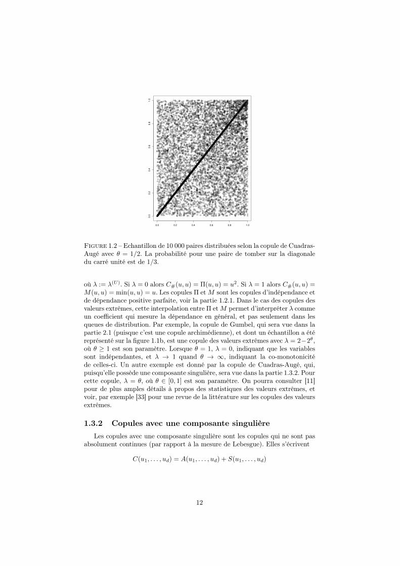
Figure 1.2 – Echantillon de 10 000 paires distribuées selon la copule de Cuadras-Augé avec θ = 1/2. La probabilité pour une paire de tomber sur la diagonaledu carré unité est de 1/3.

où λ := λ(U). Si λ = 0 alors C#(u, u) = Π(u, u) = u2. Si λ = 1 alors C#(u, u) =M(u, u) = min(u, u) = u. Les copules Π etM sont les copules d’indépendance etde dépendance positive parfaite, voir la partie 1.2.1. Dans le cas des copules desvaleurs extrêmes, cette interpolation entre Π etM permet d’interpréter λ commeun coefficient qui mesure la dépendance en général, et pas seulement dans lesqueues de distribution. Par exemple, la copule de Gumbel, qui sera vue dans lapartie 2.1 (puisque c’est une copule archimédienne), et dont un échantillon a étéreprésenté sur la figure 1.1b, est une copule des valeurs extrêmes avec λ = 2−2θ,où θ ≥ 1 est son paramètre. Lorsque θ = 1, λ = 0, indiquant que les variablessont indépendantes, et λ → 1 quand θ → ∞, indiquant la co-monotonicitéde celles-ci. Un autre exemple est donné par la copule de Cuadras-Augé, qui,puisqu’elle possède une composante singulière, sera vue dans la partie 1.3.2. Pourcette copule, λ = θ, où θ ∈ [0, 1] est son paramètre. On pourra consulter [11]pour de plus amples détails à propos des statistiques des valeurs extrêmes, etvoir, par exemple [33] pour une revue de la littérature sur les copules des valeursextrêmes.

1.3.2 Copules avec une composante singulièreLes copules avec une composante singulière sont les copules qui ne sont pas

absolument continues (par rapport à la mesure de Lebesgue). Elles s’écrivent

C(u1, . . . , ud) = A(u1, . . . , ud) + S(u1, . . . , ud)

12

avec

A(u1, . . . , ud) =

∫

[0,u1]×···×[0,ud]

∂dC(x1, . . . , xd)

∂x1 . . . ∂xd1{∂dC(x1, . . . , xd)

∂x1 . . . ∂xdexiste

}dx1 . . . dxd

étant la partie absolument continue et S = C − A la composante singulière dela copule.

La loi avec une composante singulière la plus connue est sans doute la loide Marshall-Olkin [64], voir aussi [69] section 3.1.1, dont la copule de survie estdonnée par

Cθ(u1, . . . , ud) =P [F1(X1) > u1, . . . , Fd(Xd) > ud]

=(1− u1)θ1 . . . (1− ud)θd min(u1−θ11 , . . . , u1−θd

d ),

où θ = (θ1, . . . , θd) ∈ [0, 1]d. La copule de Marshall-Olkin est, en principe 4,intéressante pour modéliser des systèmes qui présentent des « chocs ». Plus pré-cisément, soient Z1, . . . , Zd et Z0 des variables aléatoires indépendantes de loisexponentielles qui représentent les instants où les chocs arrivent dans le système,causant des dommages à ses composants. Les variables Z1, . . . , Zd représententdes chocs endogènes qui n’affectent que les composants 1, . . . , d respectivement,et Z0 représente un choc exogène qui affecte tout le système (1, . . . , d). SoientX1 = min(Z1, Z0), . . . , Xd = min(Zd, Z0) les instants où les composants 1, . . . , dsubissent un choc, qui leur est fatal. On peut alors montrer que la copule desurvie associée à (X1, . . . , Xd) est la copule de survie de Marshall-Olkin, oùles paramètres sont déterminés par les paramètres des lois exponentielles deZ1, . . . , Zd et Z0. Dans le cas bivarié, la copule de Marshall-Olkin est donnéepar

C(θ1,θ2)(u1, u2) = min(u1−θ11 u2, u1u

1−θ22 ) =

{u1−θ1

1 u2 si uθ11 ≥ uθ22 ,

u1u1−θ22 si uθ11 ≤ uθ22 ,

pour 0 ≤ θ1, θ2 ≤ 1. Pour cette copule, on peut voir facilement que même lesdérivées partielles de C(θ1,θ2) n’existent pas sur la diagonale principale du carréunité. La composante singulière est donnée par

S(u1, u2) =

∫ min(uθ11 ,u

θ22 )

0

t1/θ1+1/θ2−2dt.

En particulier, on a que P [Uθ11 = Uθ22 ] = θ1θ2/(θ1 + θ2 − θ1θ2). Dans le casoù θ1 = θ2 ≡ θ, la copule de Marshall-Olkin se réduit à la copule de Cuadras-Augé [12], donnée par

Cθ(u1, u2) = min(u1, u2) max(u1, u2)1−θ (1.7)

(cette copule peut aussi être vue comme un cas particulier de [3]). Sur la fi-gure 1.2, où un échantillon de taille 10 000 est représenté, on voit bien la com-posante singulière sur la diagonale principale du carré unité. Les chocs seraient

4. Malgré l’attrait de cette interprétation en termes de chocs, l’intérêt de la copule deMarshall-Olkin reste surtout théorique. En effet, il est difficile de trouver des publicationsprésentant des applications avec des jeux de données réelles lorsque l’on effectue des requêtespar mots clés dans les moteurs de recherche. La seule application que nous ayons trouvée [56]est plutôt décevante : elle consistait en l’analyse de 37 matchs de foot ; d’ailleurs, les auteurseux mêmes admettent que l’application était présentée uniquement pour « illustrer » leurméthode d’estimation.

13

les points de la diagonale principale. La référence originale dans lequel figure cemodèle en termes de lois exponentielles est [64].

Une autre classe de copules avec composantes singulières, et qui peuventaussi être interprétées comme des modèles avec des chocs, est donnée ci-après.La classe des copules de « Durante » [17,19] consiste en les copules de la forme

C(u1, . . . , ud) = min(u1, . . . , ud)f(max(u1, . . . , ud)), (1.8)

où f : [0, 1] → [0, 1], appelé le générateur de C, est une fonction dérivable etstrictement croissante telle que f(1) = 1 et t 7→ f(t)/t est strictement décrois-sante. L’interprétation en termes de chocs s’obtient en remarquant que (1.8)est la loi de (U1, . . . , Ud), avec Ui = max(Zi, Z0), i = 1, . . . , d ; Z1, . . . , Zd sontdes variables indépendantes distribuées selon une même loi f , et Z0 est unevariable indépendante de (Z1, . . . , Zd) distribuée selon t 7→ t/f(t). Dans le casmultivarié, puisqu’il n’y a qu’un seul générateur pour déterminer la structurede dépendance, cette classe n’est pas très utile pour les applications. Dans lecas bivarié, en revanche, la classe de copules de Durante est flexible et ma-niable (voir le chapitre 6). On peut également obtenir des copules bien connuescomme cas particuliers. Ainsi, si f(t) = t1−θ, θ ∈ [0, 1], on obtient la famille deCuadras-Augé (1.7), et si f(t) = (1− θ)t+ θ, θ ∈ [0, 1], on obtient la famille deFréchet [24], donnée par

Cθ(u1, u2) = (1− θ)Π(u1, u2) + θM(u1, u2),

et qui est la moyenne arithmétique entre la copule d’indépendance Π et la copulede la dépendance positive parfaite M . La classe de copules bivariées de Durantesera utilisée dans la construction du modèle que nous proposons au chapitre 6.En particulier, dans ce chapitre, nous construisons des copules multivariées,flexibles et maniables, dont les marges bivariées appartiennent à cette classe. Onpeut donc voir notre travail comme une extension au cas multivarié de la classedes copules bivariées de Durante plus flexible pour les applications que (1.8).

A la vue de la figure 1.2, il ne vient pas à l’esprit que l’on pourrait modéli-ser un phénomène lisse, présent dans la nature, tel que par exemple les débitsde rivières ou la quantité de pluie qui tombe sur plusieurs sites répartis dansl’espace, avec un modèle possédant une composante singulière. C’est pourtantce qu’on fait les auteurs dans [20, 77]. Leurs résultats suggèrent que certainescaractéristiques d’intérêt de la loi sous jacente ont pû être approchées par unmodèle à chocs, alors même qu’il est clair que, par exemple, la probabilité quedeux débits dans deux rivières différentes soient exactement égaux est nulle.Cette approche 5, qui s’intéresse moins à modéliser la distribution sous jacentequ’à estimer certaines caractéristiques de celle-ci, comme par exemple le niveaucritique associé à une évènement de pluie extrême (ces derniers seront vus auxchapitres 6 et 3), bien que douteuse en dimension petite, devient intéressantequand la dimension augmente. C’est aussi l’approche que nous avons suivie,comme nous le verrons au chapitre 6.

5. Cette stratégie se rapproche de la méthode « boîte noire » utilisée en machine learning.Les deux approches, « boîte noire » et « modèle », sont discutées par exemple dans [7], oùl’auteur se fait par ailleurs l’avocat de la première.

14

Chapitre 2

Modèles de copules en grandedimension

Les copules en grande dimension, ou simplement multivariées, sont plus dif-ficiles à construire que les copules bivariées. A cause de cela, le terme multivariése réfère souvent au cas où le nombre de variables d est supérieur à 2 stricte-ment. Le terme grande dimension, quand à lui, est très subjectif. La « grandedimension », telle qu’elle est parfois entendue par la communauté des chercheursdans le domaine des copules, peut commencer à partir de d = 3 1...

Dans ce chapitre, nous présentons les principaux 2 modèles de copules dela littérature. En grande dimension, il y a principalement trois familles de mo-dèles : les copules archimédiennes (partie 2.1) et leur extensions, les copules ar-chimédiennes imbriquées (2.2), les Vines (partie 2.3), et les copules elliptiques(partie 2.4).

2.1 Copules archimédiennesUne copule archimédienne est une copule qui s’écrit

C(u1, . . . , ud) = ψ(ψ−1(u1) + · · ·+ ψ−1(ud)) (2.1)

où ψ est une fonction décroissante et continue de [0,∞) dans [0, 1], strictementdécroissante sur [0, inf{x : ψ(x) = 0}), et telle que ψ(0) = 1 et ψ(x)→ 0 quandx→∞. En fait, ces conditions sur ψ sont nécessaires mais pas suffisantes. Cesdernières ont été établies dans [67]. Dans le cas où inf{x : ψ(x) = 0} =∞, (2.1)est une copule bien définie si et seulement si ψ est complètement monotone [49],c’est à dire que (−1)iψ(i)(s) ≥ 0 pour tout i et tout s ≥ 0, où ψ(i) est la i-èmedérivée de ψ. De plus, dans ce cas, on peut montrer que ψ est une transformée de

1. A l’heure des big data, on pourrait avoir du mal à cacher sa déception. Cependant, ilconvient de garder à l’esprit que ce ne sont pas les mêmes questions scientifiques qui sontposées, et que ce ne sont pas non plus les mêmes modèles qui sont utilisés. Par exemple, dansles genome-wide association studies en bioinformatique – où on analyse plusieurs milliers devariables –, on s’autorise les modèles linéaires gaussiens pour modéliser le bruit [46]. Dansle domaine des copules, l’aléa n’est pas du bruit, il est considéré comme intrinsèque, et lesmodèles linéaires gaussiens en seraient une trop mauvaise approximation.

2. cet adjectif comporte inévitablement une part de subjectivité

15

Laplace d’un vecteur strictement positif. Autrement dit, il existe une fonctionde répartition H telle que

ψ(s) =

∫ ∞

0

exp(−sy)dH(y), s ≥ 0.

En outre, dans ce cas, il existe de manière unique d fonctions de répartitionG1, . . . , Gd telles que

(2.1) =

∫ ∞

0

(G1 . . . Gd)αdH(α) = ψ

(−

d∑

i=1

logGi

).

Par exemple, la copule de Gumbel [36], donnée par

C(u1, . . . , ud) = exp{−[(− log u1)θ + · · ·+ (− log ud)

θ]1/θ}

, (2.2)

est une copule archimédienne de la forme (2.1) avec ψ−1(t) = (− log t)θ pourθ ≥ 1 (notons que c’est aussi une copule des valeurs extrêmes). La copule deClayton (1.4) est aussi une copule archimédienne avec ψ−1(t) = (t−θ−1)/θ, θ >0. Les copules archimédiennes possèdent l’avantage d’être simples, explicites etinterprétables. Ainsi, pour une copule archimédienne bivariée, le tau de Kendallest donné par

τ = 1 + 4

∫ 1

0

ψ−1(t)

(ψ−1)′(t)dt.

Par exemple, celui de la copule de Clayton vaut θ/(θ + 2). En général, le géné-rateur ψ est déterminé par un ou deux paramètre(s), dont on pourra en trouverune liste dans [69] section 4.

Les copules archimédiennes ont cependant un défaut de poids : leurs quelquesparamètres sont supposés rendre compte de toute la richesse de la structure dedépendance entre toutes les variables quelle que soit la dimension considérée.Ces copules sont échangeables, c’est à dire que

C(u1, . . . , ud) = C(uπ(1), . . . , uπ(d))

pour toute permutation π de (1, . . . , d). Ceci implique en particulier que toutesles paires de variables ont la même loi statistique.

Les applications des copules archimédiennes en grande dimension couvrent,entre autre, la modélisation et l’évaluation du risque associé à des portefeuillescontenant un grand nombre d’actifs financiers, comme dans l’exemple introductifque nous avons vu dans l’introduction, voir aussi [42] et [65]. Du fait de la pro-priété d’échangeabilité, de meilleurs résultats sont attendus si ces portefeuillessont relativement homogènes, mais, comme il est fait remarquer dans [42], lescopules archimédiennes ne sont pas utilisées pour ajuster au mieux les données ;on les utilise plutôt en vertu de leur maniabilité, d’une point de vue numériquenotamment, et on attend qu’elle résume tout de même la dépendance de manièreglobale.

2.2 Copules archimédiennes imbriquéesLes copules archimédiennes imbriquées (CAI), ou hiérarchiques, sont une

tentative d’assouplir la structure de dépendance des copules archimédiennes

16

classiques. Elles sont apparues dans [47] Section 4.2, puis ont fait l’objet d’étudesnumériques très poussées [40,68,72] et commencent à être utilisées dans plusieursapplications en finance et économétrie [43,78] et hydrologie [83].

Une CAI est une copule construite en imbriquant des copules archimédiennesles unes dans les autres. Par exemple, en dimension 3, la copule

C(u1, u2, u3) = Cψ0(u1, Cψ23(u2, u3)) (2.3)

est une CAI car la copule Cψ0prend pour second argument une autre copule

Cψ23 . En notant ψ0 et ψ23 les générateurs des copules archimédiennes Cψ0 etCψ23 , (2.3) se réécrit

C(u1, u2, u3) = ψ0

(ψ−1

0 (u1) + ψ−10 (ψ23(ψ−1

23 (u2) + ψ−123 (u3)))

). (2.4)

Le même principe s’applique pour construire des copules en plus grande dimen-sion. L’avantage par rapport aux copules archimédiennes classiques réside dansla possibilité de construire des structures de dépendance plus souples. Ainsi,dans (2.3), la loi de (U2, U3) diffère de celle de (U1, U2). Malheureusement, mêmesi cette rustine apportée aux copules archimédiennes a été l’objet de plusieursétudes (voir les références citées plus haut), elle apparait comme un bien maigreréconfort face aux problèmes qu’il reste à résoudre, et, pire, qu’elle engendre.Tout d’abord, le manque de souplesse des copules archimédiennes n’a pas étécomplétement éliminé. Par exemple, pour reprendre notre CAI (2.3), les paires(U1, U2) et (U1, U3) ont la même distribution. De plus, les fonctions qui s’écriventsous la forme (2.4) ne sont pas nécessairement des copules. Les conditions néces-saires sur les générateurs demeurent inconnues. La condition suffisante que l’ontrouve dans [47] Section 4.2 ou dans [68] est difficile à vérifier en pratique. Dansle cas particulier où les générateurs sont de la même famille, cette condition estvérifiée si la suite des paramètres des générateurs croit en descendant dans lastructure d’imbrication. Par exemple, dans les expressions (2.4) ou (2.3), celareviendrait à dire que, si on choisissait des générateurs de la famille de Gum-bel, il faudrait que les paramètres vérifient θψ0

≤ θψ23, ce qui peut être assez

restrictif.

2.3 Vines

Les modèles Vines (qui signifie « vignes, grappes, plantes grimpantes » enfrançais 3) sont basés sur la décomposition d’une densité f en un produit dedensités conditionnelles de copules bivariées multiplié par le produit des densitésmarginales.

D’après la formule de dépendance conditionnelle, une densité de probabilitéf peut se décomposer comme

f(x1, . . . , xd) = fd(xd)fd−1|d(xd−1|xd) . . . f1|2...d(x1|x2, . . . , xd). (2.5)

Chaque terme du membre de droite de (2.5) peut lui même se décomposer enun produit de densités de copules conditionnelles multiplié par un produit de

3. Cette appellation vient du fait que la représentation graphique de ces modèles, qui n’estpas abordé dans cette thèse, ressemblerait à des vignes.

17

marginales en utilisant la relation (1.2), vue dans la partie 1.1, et rappelée ci-dessous :

f(x1, . . . , xd) = c(F1(x1), . . . , Fd(xd))f1(x1) . . . fd(xd).

Ainsi, f dans (2.5) s’écrit comme un produit de densités de copules condition-nelles multiplié par un produit de densités marginales. Par exemple, en dimen-sion d = 3, une décomposition possible est :

f123(x1, x2, x3) = f3(x3)f2|3(x2|x3)f1|23(x1|x2, x3).

On réécrit les termes de la décomposition. D’abord,

f2|3(x2|x3) =f23(x2, x3)

f3(x3)

=c23(F2(x2), F3(x3))f2(x2)f3(x3)

f3(x3)

=c23(F2(x2), F3(x3))f2(x2).

Ensuite,

f1|23(x1|x2, x3) =f12|3(x1, x2|x3)f3(x3)

f23(x2, x3)

=c12|3(F1|3(x1|x3), F2|3(x2|x3))f1|3(x1|x3)f2|3(x2|x3)f3(x3)

f23(x2, x3)

=c12|3(F1|3(x1|x3), F2|3(x2|x3))f1|3(x1|x3)

=c12|3(F1|3(x1|x3), F2|3(x2|x3))c13(F1(x1), F3(x3))f1(x1).

Au final, on a

f(x1, x2, x3) =c23(F2(x2), F3(x3))c13(F1(x1), F3(x3)) (2.6)c12|3(F1|3(x1|x3), F2|3(x2|x3))f1(x1)f2(x2)f3(x3).

D’après (1.2), le produit de densités de copules conditionnelles dans (2.6) estune décomposition de la densité de la copule c associée à f . Plus la dimensionaugmente, plus le nombre de décompositions possibles augmente. Les Vines ouVines régulières [4, 5] sont un type de décompositions possible, mais encoretrop large puisque les cas particuliers appelés Vines canoniques (C-vines enanglais) et Vines « dessinables » (D-vines) ont été introduites quelques annéesaprès [58]. Les décompositions C-vines et D-vines peuvent être représentées pardes modèles graphiques consistant en une suite d’arbres. On pourra consulterles références précédentes pour plus de détails.

L’atout principal des Vines est leur grande flexibilité. En effet, passé l’étapedu choix de la décomposition de f , aucun modèle n’est encore défini. Quelleque soit la décomposition choisie, on sait qu’il existe des densités de copulesqui permettent de retrouver f exactement. En pratique, cela laisse le choix àl’utilisateur de quelles paires il va modéliser sans faire de restrictions sur f .Enfin, une fois la décomposition de f choisie, on peut faire une modélisationfine paire par paire et tirer profit de la grande richesse de la gamme de famillesde copules bivariées qui existe dans la littérature.

18

Les inconvénients des Vines sont les suivants. D’abord, dans la décomposi-tion de la densité, en pratique, on fait l’hypothèse que les copules conditionnellesne dépendent pas des valeurs conditionnantes. Par exemple, dans (2.6), la loi de(U1, U2) sachant U3 = u3, c12|3(·, ·|u3), est supposée ne pas dépendre en fait deu3, c’est à dire que la loi est la même quelles que soient les valeurs prises parU3 = u3. Cette hypothèse, faite dans la pratique afin de pouvoir choisir pourles copules conditionnelles des modèles paramétriques bivariés abondant dans lalittérature, a été discutée dans [2]. De plus, étant donné le très grand nombre depossibilités lors de la modélisation par un modèle Vines – possibilités offertesà la fois par le choix de la décomposition et le choix des familles paramétriquesà utiliser dans cette décomposition –, il n’est pas encore clair comment choi-sir le « meilleur » modèle Vines et comment tester la robustesse de ce choix.Enfin, les modèles Vines ne sont pas des modèles très maniables pour l’utilisa-teur. Les coûts de calcul nécessaires pour la simulation ou l’estimation sont plusimportants que pour d’autres modèles de copules et l’étude des propriétés dedépendance est également moins aisée. On pourra consulter [1] pour un résuméà la fois complet et accessible de la modélisation de données par Vines et [59]pour une référence plus exhaustive.

2.4 Copules elliptiquesUne copule elliptique est une copule associée à une loi elliptique. Une loi

elliptique est une transformation affine d’une loi sphérique. Un vecteur Y =(Y1, . . . , Yd) est distribué selon une loi sphérique si Y a la même loi que QYpour toute matrice orthogonale Q, c’est à dire pour toute matrice telle queQTQ = QQT = Id, où Id est la matrice identité de taille d. Autrement dit,une loi shérique est une loi invariante par rotation. La densité fY d’une loisphérique s’écrit fY (t) = g(‖t‖2), t ∈ Rd, où g est une fonction univariée appeléele générateur de densité de la loi sphérique que l’on note Sd(g). Un vecteurY ∼ Sd(g) a la représentation

Y = RS (2.7)

où S est un vecteur aléatoire distribué uniformément sur la sphère unitaire{s ∈ Rd : sT s = 1} et R ≥ 0 est une variable aléatoire indépendante de S. Unvecteur X = (X1, . . . , Xd) est distribué selon une loi elliptique Ed(µ,Σ, g) s’ils’écrit X = µ+ Σ1/2Y où Y ∼ Sd(g) et Σ est une matrice définie positive telleque Σ1/2Σ1/2 = Σ. La densité fX de X s’écrit

fX(t) = |Σ|−1/2g((t− µ)TΣ−1(t− µ)

), t ∈ Rd

et par conséquent est constante sur les ellipsoïdes de la forme {x : (x−µ)TΣ−1(x−µ) = c} pour une certaine constante c. La matrice de variance-covariance de X,lorsqu’elle existe, est donnée par E(R2)Σ/d où E est symbolise l’espérance ma-thématique et R est définie dans (2.7).

Comme nous l’avons dit plus haut, une copule elliptique en dimension d est lacopule associée à une loi elliptique Ed(µ,Σ, g). Puisqu’une copule est invariantepar standardisation des lois marginales, Ed(µ,Σ, g) et Ed(0, P, g) ont la mêmecopule, où P est la matrice de corrélation obtenue à partir de la matrice Σ. Deuxpropriétés remarquables des copules elliptiques sont les suivantes. D’abord, on

19

peut montrer [63] que le tau de Kendall d’une loi elliptique est donné par

τ =2

πarcsin(ρij), (2.8)

où ρij est l’élément de la i-ème ligne et j-ème colonne de P . Ensuite, une loielliptique Ed(µ,Σ, g) est une loi symmétrique par rapport à son rayon µ, c’està dire que X − µ est distribué comme µ−X. Cette propriété implique que lescoefficients de dépendance de queues inférieurs et supérieurs sont égaux

λ(L) = λ(U). (2.9)

Deux exemples de copules très connues sont les copules de Student et gaus-siennes. La copule de Student avec degré de liberté ν est une copule elliptiquepour laquelle

gν(x) =Γ(ν+d

2 )

Γ(ν2 )√

(πν)d

(1 +

x

ν

)−(ν+d)/2

, ν > 2, x ≥ 0

et la copule gaussienne est une copule pour laquelle

g(x) = (2π)−d/2 exp(−x/2), x ≥ 0.

Le coefficient de dépendance de queue de la copule de Student bivariée issue dela loi E2(0, ρ, gν) est donné par

λ(U) = λ(L) = 2tν+1

(−√ν + 1

√1− ρ/

√1 + ρ

),

où tν est la fonction de répartition de la loi univariée de Student standard. Lecoefficient de dépendance de queue de la copule gaussienne vaut 0 (quand le co-efficient de corrélation est strictement inférieur à 1) : elle n’a pas de dépendancede queue.

L’avantage des copules elliptiques est que l’on peut moduler l’équilibre entrela flexibilité et la maniabilité dans la modélisation. On peut par exemple réduirele nombre de paramètres en imposant une structure particulière à la matrice devariance-covariance Σ, voir par exemple [51]. De plus, la relation bijective entreles paramètres de la matrice P et les taus de Kendall (2.8) permet d’estimer cesparamètres par la méthode d’inversion du tau de Kendall, voir par exemple [16]et la partie 3.1.2 de cette thèse. Les copules elliptiques ont l’inconvénient queles coefficients de dépendance supérieurs et inférieurs sont égaux (2.9). Elles nesont donc pas des modèles réalistes pour modéliser des données présentant desdépendances de queue seulement pour les grandes valeurs ou les petites valeurs.En outre, l’ajustement de copules elliptiques à des données résulte parfois –voire souvent, lorsque le nombre de variables est grand par rapport à la taille del’échantillon – en une matrice de covariance mal conditionnée ou non inversible.Or, dans les applications, il est nécessaire de calculer l’inverse afin de pouvoirévaluer la densité [60].

Notre présentation des loi sphériques et elliptiques s’est appuyée sur les do-cuments [23] et [66] Section 3.3 que l’on pourra consulter pour plus de détails.Pour un exposé complet et accessible sur la copule de Student et ses exten-sions, comme par exemple une copule des valeurs extrêmes reliée à la copulede Student, on pourra consulter [16]. Cet article traite aussi de l’inférence. Lacopule de Student est très utilisée en finance et gestion du risque, voir parexemple [66] et ses références.

20

Chapitre 3

Inférence

Supposons que l’on dispose d’un échantillon d’une copule appartenant àune famille paramétrique (Cθ), et que l’on souhaite estimer le paramètre θ,possiblement multivarié, de notre copule. Notons notre échantillon par

(X(1)1 , . . . , X

(1)d ), . . . , (X

(n)1 , . . . , X

(n)d ), (3.1)

et remarquons que si les fonctions de répartition F1, . . . , Fd deX1, . . . , Xd étaientconnues, l’échantillon

(F1(X(1)1 ), . . . , Fd(X

(1)d )), . . . , (F1(X

(n)1 ), . . . , Fd(X

(n)d )),

serait un échantillon de la copule C elle même, et alors on pourrait se rameneraux méthodes d’inférence classiques de la statistique. Mais, puisque les margessont en fait inconnues, nous ne disposons pas d’un échantillon de notre co-pule. Pour surmonter cette difficulté, principalement deux approches peuventêtre adoptées. Dans l’approche paramétrique, on suppose que les lois marginalesappartiennent elles aussi à une famille indexée par un paramètre. Pour esti-mer les marges, il suffit alors d’estimer leur paramètre. Dans l’approche semi-paramétrique, on ne fait pas l’hypothèse que les lois marginales appartiennentà une quelconque famille. On estime les marges non paramétriquement, parexemple avec la version de l’estimateur empirique donnée par

Fi(x) =1

n+ 1

n∑

k=1

1(X(k)i ≤ x). (3.2)

Quelle que soit la façon dont on modélise et estime les lois marginales, le para-mètre θ de la copule doit ensuite être estimé. Il y principalement deux stratégies.La première est basée sur la maximisation d’une certaine fonction de vraisem-blance, et la deuxième est une méthode des moments basée sur les coefficientsde dépendance. Si l’on souhaite se passer de l’hypothèse selon laquelle la co-pule appartient à une famille paramétrique, il faut estimer la copule avec desméthodes non-paramétriques. Puisque ces méthodes ont peu de chances de suc-cès en grande dimension, nous ne les aborderons pas en détail, mais donnonsquelques références à la littérature.

La suite de ce chapitre est organisée comme suit. La partie 3.1 traite del’estimation de copules, en présentant les méthodes basées sur la vraisemblance

21

(partie 3.1.1) et sur les coefficients de dépendance (partie 3.1.2). Pour les mé-thodes non paramétriques, les références à la littérature sont données dans lapartie 3.1.3. La partie 3.2 traite brièvement des tests d’adéquation.

3.1 Estimation

3.1.1 La méthode du maximum de vraisemblanceLa densité associée à notre échantillon (3.1) a été donnée dans (1.2) ; nous

la rappelons ci-dessous :

f(x1, . . . , xd; θ) = c(F1(x1), . . . , Fd(xd); θ)

d∏

i=1

fi(xi), (3.3)

où c est la densité de la copule d’intérêt, Fi sont les fonctions de répartitionmarginales et fi les densités. Ci-dessous, les méthodes présentées, paramétriqueset semi-paramétriques, cherchent toutes les deux à maximiser une approxima-tion de la vraisemblance basée sur (3.3). La différence entre les deux méthodestient au fait que dans l’approche paramétrique, nous supposons que les margesF1, . . . , Fd appartiennent à une certaine famille paramétrique, ce qui n’est pasle cas de méthode semi-paramétrique. Evidemment, l’intérêt de l’approche pa-ramétrique réside dans le fait que, si le modèle ajusté pour les lois marginalesest raisonnable, cette approche permet une réduction de la variabilité et uneaugmentation de la maniabilité du modèle. En revanche, si le modèle est malajusté, les résultats peuvent donner lieu à des interprétations fausses [21]. C’estpour cette raison que l’approche semi-paramétrique est intéressante.

L’approche paramétrique suppose que chaque marge Fi appartient à unefamille de lois indexée par un paramètre αi. Ainsi, la densité (3.3) se réécritcomme

f(x1, . . . , xd;α1, . . . , αd; θ) = c(F1(x1;α1), . . . , Fd(xd;αd); θ)

d∏

i=1

fi(xi;αi).

(3.4)Pour estimer le vecteur des paramètres (α1, . . . , αd, θ), on peut vouloir maximi-ser la vraisemblance stricto sensu

L(α1, . . . , αd, θ) :=

n∏

k=1

f(X(k)1 , . . . , X

(k)d ;α1, . . . , αd, θ).

Cependant, cette vraisemblance peut être compliquée, voire impossible à cal-culer, ou alors l’optimisation numérique peut être trop lente ou trop complexe.Dans ces situations, on fera appel à une méthode en deux étapes, qui tire profitde la représentation (3.4). Avec cette méthode, appelée la méthode IFM (Infe-rence Functions for Margins, [47], Section 10), on procède en deux étapes.1) Le paramètre αi est estimé par αi en maximisant la vraisemblance marginale

Li(αi) =

n∏

k=1

fi(X(k)i ;αi).

22

2) Une fois les paramètres marginaux estimés dans l’étape précédente, le vecteurde paramètres θ de la copule est estimé par θ en maximisant la partie de lavraisemblance qui dépend de θ, c’est à dire que l’on maximise

L(θ) =

n∏

k=1

c(F1(X(k)1 ; α1), . . . , Fd(X

(k)d ; αd); θ).

L’estimateur IFM est consistant et asymptotiquement normal sous certainesconditions de régularité, voir par exemple [82]. L’approche IFM est intéressanted’un point de vue numérique car l’optimisation par ordinateur a plus de chancesde succès que la maximisation de la vraisemblance stricto sensu. Au vu de cequi précède, on peut se demander quelle est l’efficacité relative de l’estimateurIFM par rapport à l’estimateur du maximum de vraisemblance. Dans [47] sec-tion 10, il est suggéré de comparer (numériquement) les matrices asymptotiquesde variance-covariances des deux estimateurs, ou bien de comparer les deuxestimateurs au moyen de simulations numériques. Dans les comparaisons pourquelques modèles faites dans [47], l’auteur rapporte une efficacité relative prochede 1, où l’efficacité relative a été mesurée comme le rapport de l’erreur quadra-tique moyenne de l’estimateur IFM avec celle de l’estimateur du maximum devraisemblance.

L’approche semi-paramétrique ne fait pas l’hypothèse que les marges F1, . . . , Fdappartiennent à une quelconque famille paramétrique. On les estime directementpar l’estimateur non paramétrique donné dans (3.2), rappelé ci-dessous,

Fi(x) =1

n+ 1

n∑

k=1

1(X(k)i ≤ x).

Pour estimer θ, on remplace les marges par leur estimation dans (3.3), et onmaximise la partie de la vraisemblance faisant intervenir θ, c’est à dire,

L(θ) =

n∏

k=1

c(F1(X(k)1 ), . . . , Fd(X

(k)d ); θ).

L’estimateur qui en résulte est consistant et asymptotiquement normal sous desconditions de régularité peu restrictives, voir [26]. Toutefois, malgré ces pro-priétés de convergence, il n’est pas, en général, efficace [32], sauf dans le cas dela copule gaussienne bivariée [50]. La construction d’estimateurs asymptotique-ment efficaces est un sujet de recherche très récent, se focalisant pour l’instantsur les modèles gaussiens : l’obtention d’une borne inférieure pour la matricede variance-covariance asymptotique, et la preuve que cette borne pouvait êtreatteinte par un estimateur semi-paramétrique a été réalisé dans [44]. Dans [81],les auteurs ont construit explicitement un estimateur atteignant la borne infé-rieure.

3.1.2 La méthode des moments basée sur les coefficientsde dépendance

Dans la littérature, l’estimation basée sur les moments est souvent entenduecomme un nom générique se référant en fait à la méthode basée sur l’inversion

23

du rho de Spearman ou du tau de Kendall (qui peuvent en effet se voir de lasorte). Ces méthodes tirent profit de la relation, plus ou moins explicite, qu’ilpeut y avoir entre le rho de Spearman et le tau de Kendall et le paramètre dela copule θ. Nous avons vu dans la partie 1.2.2 la définition de ces coefficientsde dépendance. La version empirique de ces coefficients pour la paire (Xi, Xj)est respectivement donnée par

ρi,j =

∑nk=1

(U

(k)i − U i

)(U

(k)j − U j

)

[∑nk=1

(U

(k)i − U i

)2∑nk=1

(U

(k)j − U j

)2]1/2

, et (3.5)

τi,j =

(n

2

)−1∑

k<l

sign(

(X(k)i −X(l)

i )(X(k)j −X(l)

j )), (3.6)

où U(k)i = Fi(X

(k)i ), Ui =

∑nk=1 U

(k)i /n, i = 1, . . . , d et sign(x) = 1 si x > 0,

−1 si x < 0 et 0 si x = 0. Depuis [39], on sait que ces deux estimateurs sontconsistants et asymptotiquement non biaisés et normaux. Dans le cas bivarié(d = 2) et lorsqu’il n’y a qu’un seul paramètre réel à estimer, la méthode parinversion du tau de Kendall s’applique à faire correspondre l’estimation sous lemodèle avec son estimation empirique. En d’autres termes, l’estimateur θ vérifie

τ(θ) = τ1,2,

et donc, si θ 7→ τ(θ) est inversible

θ = τ−1(τ1,2). (3.7)

Les propriétés asymptotiques de (3.7) s’obtiennent immédiatement d’après lespropriétés asymptotiques de τ1,2 lui même et la méthode « delta » (delta-methoden anglais, voir par exemple [84]). Si au lieu du tau de Kendall, on souhaite uti-liser le rho de Spearman, voire d’autres coefficients de dépendance, la méthodefonctionne de la même manière. Notons enfin que la méthode par inversion dutau de Kendall ou du rho de Spearman est semi-paramétrique, puisque dansles expressions (3.6) et (3.5), les marges F1, . . . , Fd sont implicitement estiméespar (3.2). On pourra consulter [25] pour une introduction accessible de ces mé-thodes, et [30] pour plus de détails dans le cas du tau de Kendall et des copulesarchimédiennes. Des généralisations de la méthode des moments basée sur lescoefficients de dépendance ont été proposées dans la littérature pour pouvoirestimer des copules plus complexes.

Copules elliptiques. La méthode par inversion du tau de Kendall est trèsutilisée pour estimer les paramètres de la matrice de corrélation P des copuleselliptiques (vues dans la partie 2.4), car, pour chaque marge bivariée de cescopules, il y a une correspondance un à un entre l’élément de la i-ème ligneet de la j-ème colonne de P et le tau de Kendall (2.8). Voir par exemple [66]chapitre 5.5, ou [16] dans le contexte des copules de Student. Dans le cas d’unmodèle parcimonieux, c’est à dire lorsque l’on impose une structure à la matricede variance-covariance, cette correspondance est brisée. Cependant, on peut toutde même estimer le vecteur des paramètres en minimisant la fonction (3.8),comme expliqué ci-dessous.

24

Le cas multivarié, mais avec un seul paramètre réel. Au delà du casbivarié (d > 2), mais lorsqu’il n’y a qu’un seul paramètre à estimer – c’est le caspar exemple des copules archimédiennes, voir la partie 2.1 – une extension a étéétudiée dans [27]. Comme il y a cette fois plusieurs paires, les auteurs étudientl’estimateur qui vérifie

τ(θ) =1

d(d− 1)/2

∑

i<j

τi,j ,

où les τi,j sont les taus de Kendall empiriques des paires (Xi, Xj). Toujours ense basant sur [39], on peut établir les propriétés asymptotiques de θ.

Le cas général. L’estimateur revêt la forme

θ = arg minθ∈Θ

(r − r(θ))T W (r − r(θ)) , (3.8)

où W est une matrice de poids et r = (r1,2, . . . , rd−1,d), r = (r1,2, . . . , rd−1,d).Pour construire l’estimateur, ri,j doit être remplacé par un coefficient de dé-pendance entre Xi et Xj et ri,j par sa contrepartie empirique. Par exemple,le cas des copules elliptiques avec ri,j = Cor(Xi, Xj) a été considéré dans [51].Le cas plus général où ri,j peut être n’importe quel coefficient de dépendance(sous des conditions de convergence de sa contrepartie empirique) a été considérédans [71]. Dans cet article, les auteurs partent du principe que les coefficientsde dépendance ri,j ne peuvent pas être calculés, même numériquement. Leurpoint de vue est motivé par le fait que les copules qu’ils considèrent [70,71] sontdéfinies implicitement. Pour résoudre ce problème, ils proposent d’approcher ri,jpar simulation. Nous renvoyons à [71] pour plus de détails. L’estimateur a étéprouvé consistant et asymptotiquement normal sous des conditions de régulariténaturelles.

Dans le cas général, pour établir les propriétés asymptotiques de (3.8), les au-teurs de [71] ont besoin de l’existence (et de la continuité) des dérivées partiellesdes copules sous jacentes. Donc, si l’on souhaite estimer les paramètres de co-pules pour lesquelles ces dérivées n’existent pas, comme par exemple les copulessingulières vues dans la partie 1.3.2 et le chapitre 6, il n’y a aucun argumentthéorique pour utiliser cette méthode. Dans ce contexte, l’objet du chapitre 5est de lever cette hypothèse. Ainsi, nous pouvons estimer les paramètres descopules proposées dans le chapitre 6.

3.1.3 Les méthodes non paramétriquesLa plupart des méthodes non-paramétriques sont basées sur la copule empi-

rique [14] définie par

C(u1, . . . , ud) = F (F−11 (u1), . . . , F−1

d (ud)),

où F est un estimateur de la fonction de répartition – par exemple la fonctionde répartition empirique, ou bien un estimateur construit à l’aide d’un noyau –,et F−1

i est un estimateur non paramétrique de la fonction quantile généralisée,par exemple, F−1

i (x) = inf{y : Fi(y) ≥ x}. La consistance et normalité asymp-totique de la copule empirique ont été établies dans [22] sous des conditions de

25

régularité sur les dérivées partielles. Voir aussi [80] pour la possibilité de relaxercertaines de ces conditions.

Dans le cas des copules des valeurs extrêmes, on peut envisager d’autresméthodes qui se basent sur une représentation de celles-ci en terme d’une fonc-tion de dépendance univariée qui doit vérifier certaines propriétés, voir parexemple [33]. Dans le cas où les lois marginales Fi sont supposées connues,on pourra consulter [9, 15,38] dans le cas bivarié, et [73] dans le cas multivarié.Dans le cas où elles sont supposées inconnues, voir [8, 31] dans le cas bivariéet [34,35] dans le cas multivarié.

Récemment, les méthodes non paramétriques ont été utilisées pour estimerdes copules Vines [37]. Puisque les copules Vines sont construites à partir decopules bivariées, ces méthodes ont de meilleures chances de succès dans ce cas.

Enfin, la copule de Durante vue dans la partie 1.3.2 a aussi été le terrain dejeux de méthodes non paramétriques, voir [18].

3.2 TestsEtant choisie une famille paramétrique pour la copule d’intérêt, il est critique

de se demander si ce choix était le bon. Pour répondre à cette question, on faitdonc le test H0 : « la copule appartient à la famille paramétrique choisie » contreH1 : « la copule n’appartient pas à la famille ». D’après [6,29], les tests les pluspuissants sont basés sur le processus

√n(C − Cθ),

où C est la copule empirique et Cθ est l’estimation paramétrique obtenue sousH0. En particulier, la statistique de test de Cramér-von Mises

∫

[0,1]dn(C − Cθ)dC

donne les meilleurs résultats. Pour obtenir des p valeurs, on peut recourir aubootstrap [28] mais au prix d’un coût de calcul élevé. Une alternative, appeléeapprochemultiplier, proposée dans [53,55] et implémentée dans le paquet copula[54] du logiciel R , permet de réduire ce coût. Enfin, des tests existent pourévaluer si une copule est une copule des valeurs extrêmes, voir par exemple [52].

26

Deuxième partie

Deux nouvelles classes decopules et leur estimation

27

Chapitre 4

Un modèle de copules basésur des produits de copulesbivariées

Un produit de copules n’est pas, en général, une copule. Un contre exempleévident serait de prendre C1(u, v) = C2(u, v) = uv la copule d’indépendance etde remarquer que

C(u, v) = C1(u, v)C1(u, v) = u2v2 (4.1)

n’est pas une copule, car ses marges ne sont pas uniformes. Toutefois, en mo-difiant les arguments des copules amenées à composer le produit, et en leurimposant certaines contraintes, il est possible de réussir à ce que ce derniervérifie toutes les conditions pour être une copule bien définie. Dans l’exempleprécédent (4.1), il suffit d’élever les arguments de C1 et C2 à la puissance 1/2,c’est à dire C(u, v) = C1(u1/2, v1/2)C1(u1/2, v1/2) = uv pour que C soit bienune copule. De manière générale, considérons le produit

C(u1, . . . , ud) =

K∏

e=1

Ce (ge1(u1), . . . , ged(ud)) (4.2)

où les gei sont des fonctions de [0, 1] dans [0, 1] et les Ce sont des copules arbi-traires. Dans [62], l’auteur donne des conditions suffisantes sur les gei pour que(4.2) soit une copule bien définie. Dans la suite, nous parlerons donc de produitde copules en sous entendant le produit (4.2), et pas le produit stricto sensu.Entre autre, gei doit satisfaire la contrainte

K∏

e=1

gei(v) = v, v ∈ [0, 1]. (4.3)

Par exemple, si on prend la forme paramétrique gei(v) = vθei , la contraintedevient

K∑

e=1

θei = 1.

Au total, il y a d contraintes de la sorte à satisfaire, une pour chaque indice i.

28

La classe de copules (4.2) n’a pour l’instant un intérêt que théorique. En effet,en pratique, les problèmes apparaissent, comme le choix des gei et la satisfactiondes contraintes (4.3). En outre, comment construire un modèle parcimonieux àpartir de (4.2) ? Même si de telles copules pouvaient être construites, commentaborder l’inférence ? En effet, la méthode du maximum de vraisemblance néces-site de calculer la densité de la copule étudiée. Puisque la copule qui nous occupeest un produit, il est clair que son calcul sera très complexe. Même si, du fait desdifficultés énoncées plus haut, peu de modèles ont été construits en pratique,on citera tout de même [20], où les auteurs utilisent (4.2) pour construire descopules des valeurs extrêmes. Cependant, dans ces travaux, les contraintes surles paramètres n’ont pas pu être levées dans le cas où l’on souhaite un paramètrepar paire de variables.

Dans ce contexte, notre contribution s’articule autour de deux axes. D’unepart, nous proposons une classe de copules construite à partir de produits decopules bivariées et dont les contraintes (4.3) sont automatiquement satisfaites.D’autre part, nous faisons le lien avec un algorithme message-passing récent [45]qui permet de calculer la densité associée à un un produit de fonctions de ré-partition, et donc, a fortiori, d’un produit de copules. Nous montrons dans leThéorème 1 de notre article que cette nouvelle classe est obtenue avec seulementdeux hypothèses naturelles. Notre copule s’écrit

C(u1, . . . , ud) =∏

{ij}∈ECij(u

1/nii , u

1/njj ), (4.4)

où les Cij sont des copules complètement arbitraires, E est l’ensemble des ar-rêtes {ij} d’un graphe arbitraire ({1, . . . , d}, E) et nk est le nombre de voisinsdu sommet k dans ce graphe. Par exemple, avec E = {{12}, {24}, {23}, {35}}comme sur la Figure 1 de l’article, notre copule s’écrit

C(u1, u2, u3, u4, u5) =C12(u1, u1/32 )C24(u

1/32 , u4)C23(u

1/32 , u

1/23 )C35(u

1/23 , u5).

La marginale bivariée de (4.4) associée aux variables indexées par k et l s’écrit

Ckl(uk, ul) =

{u

(nk−1)/nkk u

(nl−1)/nll Ckl(u

1/nkk , u

1/nll ) si {kl} ∈ E,ukul sinon.

A la vue de la formule du dessus, il apparait immédiatement que deux variablesne sont pas connectées dans le graphe associé au modèle sont marginalementindépendantes. Dans l’article, nous montrons par ailleurs que les coefficientsde dépendance des marginales bivariées sont bornés, et les bornes sont d’au-tant plus sévères que le graphe est connecté. L’utilisateur d’un tel modèle doitalors faire face à un compromis. D’un côté, il souhaite connecter les variablesafin qu’elles ne soient pas marginalement indépendantes, et de l’autre, plus cesvariables sont connectées, plus les dépendances modélisées sont faibles. L’in-férence de la copule (4.4) peut se faire par maximum de vraisemblance, bienque son expression s’écrive sous la forme d’un produit, grâce à l’utilisation d’unalgorithme de message-passing [45] qui tire profit de la structure de grapheassociée à la copule. Nous donnons l’intuition de cet algorithme récent dansl’appendice de notre article, et nous l’avons implémenté dans notre cas. Cepaquet R est disponible librement sur le serveur du CRAN [87]. L’article pré-senté ci-dessous a été soumis pour publication, et est disponible à l’adressehttp://hal.archives-ouvertes.fr/hal-00910775.

29

A class of multivariate copulas based on products

of bivariate copulas

Gildas Mazo (gildas.mazo@free.fr), Stephane Girardand Florence Forbes

Inria and Laboratoire Jean Kuntzmann, Grenoble, France

Abstract

Copulas are a useful tool to model multivariate distributions. Whilethere exist various families of bivariate copulas, much fewer has beendone when the dimension is higher. In this paper we propose a class ofmultivariate copulas based on products of transformed bivariate copulas.No constraints on the parameters refrain the applicability of the proposedclass. Furthermore the analytical forms of the copulas within this classallow to naturally associate a graphical structure which helps to visualizethe dependencies and to compute the likelihood efficiently even in highdimension.

Keywords: maximum-likelihood inference, graphical models, message-passingalgorithm, multivariate, copula.

1 Introduction

The modelling of random multivariate events is a central problem in variousscientific domains and the construction of multivariate distributions able toproperly model the variables at play is challenging. A useful tool to deal withthis problem is the concept of copulas. Let (X1, . . . , Xd) be a random vectorwith distribution function F . Let Fi be the (continuous) marginal distributionfunction of Xi, i = 1, . . . , d. By Sklar’s Theorem [17], there exists a uniquefunction C such that

F (x1, . . . , xd) = C(F1(x1), . . . , Fd(xd)). (1)

This function C is called the copula of F and is the d-dimensional distributionfunction of the random vector (F1(X1), . . . , Fd(Xd)). For a general account oncopulas, see, e.g. [16]. Copulas are interesting since they permit to impose adependence structure on pre-determined marginal distributions.

While there exist many copulas in the bivariate case, it is less clear howto construct copulas in higher dimension. In the presence of non-Gaussianityand/or tail dependence, various constructions have been adopted, such as, forinstance, Archimedean copulas [9], Vines [1] or elliptical copulas [5]. BecauseArchimedean copulas possess only a few parameters, they lack flexibility in high-dimension. Vines, on the opposite, achieve greater flexibility but at the priceof increased complexity in the modeling process. The use of elliptical copulas

30

goes together with assuming a similar dependence pattern among all pairs ofvariables. This may be undesirable in applications. Moreover, they have ingeneral as many as O(d2) parameters and it is difficult to carry out maximumlikelihood inference [3].

Another approach [14] aims at constructing a multivariate copula as a prod-uct of transformed bivariate copulas. This approach possesses several advan-tages. A probabilistic interpretation is available and thus the generation ofrandom vectors is straightforward. The resulting copula is explicit, leading toexplicit bounds on dependence coefficients of the bivariate marginals. The classof copulas which can be constructed from this approach is large and can covera wide range of dependencies. Finally the analysis of extreme values can beperformed by constructing extreme-value copulas.

However, although many copulas with different features can be built, theuse of this approach for practical applications remains challenging. Indeed, twopitfalls render inference difficult: first, they are constraints on the parameters,and second, the product form complicates the computation of the density –hence, of the potential likelihood – even numerically.

The main contribution of this paper is to revisit the product of transformedcopulas in order to propose a new multivariate copula model of practical inter-est. First, there are no constraints on the parameters anymore. Moreover, agraphical structure associated to the copulas within this class permits to visu-alize the dependencies and to efficiently compute the likelihood, even in highdimension.

The rest of this paper is organized as follows. Section 2 reviews the productof transformed copulas and important properties such as random generation andthe ability to construct extreme-value models. Section 3 presents the new copulamodel and enlightens the link with the product of transformed copulas. Section 4discusses the dependence properties of bivariate marginals of the proposed classby providing bounds on some of the most popular dependence coefficients suchas Spearman’s rho, Kendall’s tau, and tail dependence coefficients. In Section5, we apply the proposed copula model to a simulated and a real dataset. Theappendix gathers the proofs of this paper.

2 Product of transformed copulas

It is easily seen that a product of copulas is not a copula in general. Nonethelessthe next theorem due to Liebscher [14] shows that, up to marginal transforma-tions, a product of copulas can lead to a well defined copula.

Theorem 1. Assume C1, . . . , CK : [0, 1]d → [0, 1] are copulas. Let gei :[0, 1] → [0, 1] for e = 1, . . . ,K, i = 1, . . . , d be functions with the propertythat each of them is strictly increasing or is identically equal to 1. Supposethat

∏Ke=1 gei(v) = v for v ∈ [0, 1], i = 1, . . . , d, and limv→0 gei(v) = 0 for

e = 1, . . . ,K, i = 1, . . . , d. Then

C(u1, . . . , ud) =

K∏

e=1

Ce (ge1(u1), . . . , ged(ud)) (2)

is also a copula.

31

The probabilistic interpretation of (2) is as follows. Let

(U(1)1 , . . . , U

(1)d ), . . . , (U

(K)1 , . . . , U

(K)d )

be K independent random vectors having distribution function C1, . . . , CK re-spectively. Let gei, e = 1, . . . ,K, i = 1, . . . , d be as in Theorem 1 and defineg−1ei (v) := 0 for v ≤ gei(0) and Ji = {e ∈ {1, . . . ,K} : gei 6= 1}. Then C is thejoint distribution function of the random vector

(maxe∈J1

g−1e1 (U(e)1 ), . . . ,max

e∈Jdg−1ed (U

(e)d )

). (3)

If there exists a random generation procedure for Ce, e = 1, . . . ,K then thanksto (3) a random generation procedure for C can be derived as well.

The statistical analysis of extreme values should theoretically be carriedout with the help of extreme-value copulas [8]. Recall that a copula C# is anextreme-value copula if there exists a copula C such that

C#(u1, . . . , ud) = limn↑∞

Cn(u1/n1 , . . . , u

1/nd ), (4)

for every (u1, . . . , ud) ∈ [0, 1]d. A copula C# is said to be max-stable if for everyinteger n ≥ 1 and every (u1, . . . , ud) ∈ [0, 1]d

Cn#(u1/n1 , . . . , u

1/nd ) = C#(u1, . . . , ud).

Extreme-value copulas correspond exactly to max-stable copulas [8]. Theorem 1can be used to construct extreme-value copulas as shown in the next propositiondue to [4].

Proposition 1. In (2), let gei(v) = vθei , v ∈ [0, 1] with θei ∈ [0, 1] and∑Ke=1 θei = 1 for i = 1, . . . , d. If Ce, e = 1, . . . ,K is max-stable then so is

C.

Out of the context of extreme values, applications of Theorem 1 can befound, for instance, in the analysis of directional dependence [13] (K = d = 2),finance [2] (K = d = 2) and hydrology [4] (K = 2, d = 3).

We are not aware of applications of Theorem 1 in practice when K > 2 ord > 3. As pointed out in the introduction, the product form (2) renders the

density ∂dC(u1,...,ud)∂u1...∂ud

, hence the likelihood, complicated to compute even numer-

ically. Furthermore, the constraints∏Ke=1 gei(v) = v, v ∈ [0, 1], i = 1, . . . , d in

Theorem 1 are not easy to deal with in practice.The next section aims at overcoming these drawbacks.

3 Product of transformed copulas revisited

The product over e ∈ {1, . . . ,K} in (2) can be taken over e ∈ E, where E is anarbitrary finite set, yielding

C(u1, . . . , ud) =∏

e∈ECe (ge1(u1), . . . , ged(ud)) . (5)

32

Figure 1: Graphical representation of the set E = {{12}, {24}, {23}, {35}}.N(1) = {{12}}, N(2) = {{12}, {23}, {24}}, N(3) = {{23}, {35}}, N(4) ={{24}} and N(5) = {{35}}.

In particular, an element e ∈ E can represent a pair of the variables at play.More precisely, let U1, . . . , Ud be d standard uniform random variables. Denoteby {ij} the index of the pair (Ui, Uj) and let E ⊂ {{ij} : i, j = 1, . . . , d, j > i}be a subset of the set of the pair indices. The cardinal of E, denoted by |E|, isless or equal to d(d− 1)/2. The pair index e ∈ E is said to contain the variableindex i if e = {ik} for k 6= i. Let us introduce N(i) = {e ∈ E : e contains i}.N(i) is called the set of neighbors of i and has cardinal |N(i)| = ni. It is naturalto associate a graph to the set E as follows: an element e = {ij} ∈ E is anedge linking Ui and Uj in the graph whose nodes are the variables U1, . . . , Ud.The example E = {{12}, {24}, {23}, {35}} is illustrated in Figure 1. For u =(u1, . . . , ud) ∈ [0, 1]d, consider the functional

C(u1, . . . , ud) =∏

{ij}∈ECij(u

1/nii , u

1/njj ), (6)

where the Cij ’s are bivariate copulas. Keeping in mind the graphical repre-sentation, C in (6) is a product over the edges. For instance, when E ={{12}, {24}, {23}, {35}} as in Figure 1, (6) writes

C(u1, u2, u3, u4, u5) =C12(u1, u1/32 )C24(u

1/32 , u4)C23(u

1/32 , u

1/23 )C35(u

1/23 , u5).

In the following, (6) is referred to as the Product of Bivariate Copulas (PBC)copula, or PBC model. The next theorem establishes that (6) is a copula andmakes the link with Theorem 1.

Theorem 2. If in (5):

(i) for e = {ij} ∈ E, Ce takes exactly two arguments non identically equal toone, namely, gei and gej, and

(ii) for i = 1, . . . , d and e ∈ N(i), gei does not depend on e;

33

then the only copula which can be constructed from (5) is the PBC model (6),where Cij is defined by

Cij(u, v) = C{ij}(1, . . . , 1, u, 1, . . . , 1, v, 1, . . . , 1), (u, v) ∈ [0, 1]2,

and where in (1, . . . , 1, u, 1, . . . , 1, v, 1, . . . , 1), u and v are at the i-th and j-thpositions respectively.

Condition (i) in Theorem 2 simply means that only bivariate copulas areallowed in the construction. The simplification (ii) achieves two goals: firstto reduce the number of parameters (an important feature in high-dimension),and second to intrinsically satisfy the constraints

∏e∈E gei(v) = v, v ∈ [0, 1], i =

1, . . . , d in the assumptions of Theorem 1. If assumption (ii) in Theorem 2 wasnot made, one could take gei(v) = vθei , e ∈ E, i = 1, . . . , d, θei ∈ [0, 1] with theconstraints ∑

e∈N(i)

θei =∑

k:{ki}∈Eθki,i = 1, i = 1, . . . , d. (7)

These constraints would be difficult to handle in practice, and, furthermore,the number of parameters would increase quadratically with the dimension.Indeed, one would have (|E| − 1)d parameters θei plus an additional number|E| of parameters for each copula Ce. If the graph associated to E is a tree, forinstance, then |E| = d− 1, yielding O(d2) parameters. As a comparison, in thePBC model (6), there are no constraints and only O(d) parameters in total.

From (1), the PBC copula (6) is associated to a distribution function F withcontinuous marginals Fi, i = 1, . . . , d, such that

F (x1, . . . , xd) = C(F1(x1), . . . , Fd(xd)), (x1, . . . , xd) ∈ Rd. (8)

By substituting (6) into (8), it is easy to see that F writes

F (x1, . . . , xd) =∏

{ij}∈EFij(xi, xj), (x1, . . . , xd) ∈ Rd, (9)

where Fij , {ij} ∈ E, is a bivariate distribution function such that the first(respectively the second) marginal Fij,1 (respectively Fij,2) only depends on i(respectively j). It is interesting to note that the converse is also true as statedin the following proposition.

Proposition 2. The distribution function corresponding to the PBC copula (6)writes as F in (9). Conversely, the copula corresponding to the distributionfunction F in (9) writes as the PBC copula (6).

4 Dependence properties and max-stability

Let C be the PBC copula (6). First the dependence properties of a pair (Uk, Ul)whose copula is the bivariate copula Ckl(uk, ul) = C(1, . . . , 1, uk, 1, . . . , 1, ul, 1, . . . , 1)are studied. The conditions under which the PBC model (6) is an extreme-valuecopula are given afterwards.

Proposition 3. The bivariate marginal Ckl is given by

Ckl(uk, ul) =

{u(nk−1)/nkk u

(nl−1)/nll Ckl(u

1/nkk , u

1/nll ) if {kl} ∈ E,ukul otherwise.

(10)

34

Example 1. If in (10) Ckl is a Marshall-Olkin copula (see for instance [16],p.53) with parameters 0 ≤ α, β ≤ 1 (denoted by MO(α, β)), that is,

Ckl(uk, ul) = min(u1−αk ul, u1−βl uk),

then Ckl is MO(α/nk, β/nl). If α = β then Ckl is a Cuadras-Auge copulaand Ckl is MO(α/nk, α/nl). If α = β = 0 then both Ckl and Ckl are theindependence copula. If α = β = 1 then Ckl is the Frechet upper bound copulaand Ckl is MO(1/nk, 1/nl).

Remark 1. If in (10) one puts κ = 1/nk and λ = 1/nl, then the copulas takethe form Ckl(uk, ul) = u1−κk u1−λl Ckl(u

κk , u

λl ). This class of copulas, sometimes

referred to as Khoudraji copulas, was proposed in [6] Proposition 2.

Let (U, V ) be a random vector with copula C. The dependence between Uand V is positive if, roughly speaking, U and V tend to be large or small to-gether. Below are recalled a few definitions of statistical concepts about positivedependence. The copula C has the TP2 (totally positive of order 2) property ifand only if

C(u1, u2)C(v1, v2) ≥ C(u1, v2)C(v1, u2), for all u1 < v1 and u2 < v2. (11)

Also, C is said to be PQD (positive quadrant dependent) if C(u, v) ≥ uv for all(u, v) ∈ [0, 1]2. The random variable V is said to be LTD (left tail decreasing)in U if for all v ∈ [0, 1], the function u 7→ P (V ≤ v|U ≤ u) is decreasing inu. The dependence between U and V can be quantified through dependencemeasures such as the Kendall’s tau or Spearman’s rho respectively given by

τ =4

∫

[0,1]2C(u, v) dC(u, v)− 1, (12)

ρ =12

∫

[0,1]2C(u, v) du dv − 3. (13)

The dependence in the upper and lower tails can be respectively measured with

λ(U) = limu↑1

1− 2u+ C(u, u)

1− u ∈ [0, 1], λ(L) = limu↓0

C(u, u)

u∈ [0, 1].

See [16] and [12] for further details about these concepts. Let us denote by τkl,

ρkl, λ(U)kl and λ

(L)kl the Kendall’s tau, Spearman’s rho, upper tail dependence

coefficient and lower tail dependence coefficient of the copula Ckl in (10) re-spectively. As shown in Proposition 3, Ckl is a bivariate marginal of the PBCcopula (6) and one may apply the results of [14] to obtain the following.

Proposition 4. If in (10) Ckl is TP2, LTD or PQD then Ckl is also TP2,LTD or PQD respectively.

Explicit bounds in terms of the number of neighbors for the dependencecoefficients of PBC bivariate marginals are given in the next proposition. Thebehavior of (10) when the number of neighbors tends to infinity is also studied.

35

Proposition 5. We have λ(L)kl = 0 and λ

(U)kl ≤ min(1/nk, 1/nl). The lower and

upper bounds for ρkl and τkl are respectively given by

aρ(nk, nl) ≤ ρkl ≤ bρ(nk, nl),aτ (nk, nl) ≤ τkl ≤ bτ (nk, nl),

with

aρ(nk, nl) =6β(2nk − 1, 2nl − 1)nknl

(2nk + 2nl − 1)(nk + nl − 1)− 3

(2nk − 1)(2nl − 1),

bρ(nk, nl) =3

2nk + 2nl − 1,

aτ (nk, nl) =β(2nl − 1, 2nk − 1)

nk + nl − 1− 2

(2nk − 1)(2nl − 1),

bτ (nk, nl) =1

nk + nl − 1,

where β denotes the β-function, β(x, y) =∫ 1

0tx−1(1− t)y−1dt. Furthermore, as

max(nk, nl)→∞, we have Ckl(u, v)→ uv for all (u, v) ∈ [0, 1]2.

The above results show that we are facing a tradeoff: on the one hand, thelarger the cardinal of E (or the more connected the graph associated to E), theless the pairs in E are able to model strong dependencies. On the other hand,the smaller the cardinal of E, the more there are independent pairs (since thereare less pairs in E). To illustrate Proposition 5, numerical values of the boundsare computed in Table 1 for different numbers of neighbors (nk, nl).

coefficient ρkl τkl λkl(nk, nl)(1, 2) [−0.60, 0.60] [−0.50, 0.50] [0.00, 0.50](2, 2) [−0.30, 0.43] [−0.21, 0.33] [0.00, 0.50](1, 3) [−0.43, 0.43] [−0.33, 0.33] [0.00, 0.33](2, 3) [−0.19, 0.33] [−0.13, 0.25] [0.00, 0.33](3, 3) [−0.12, 0.27] [−0.08, 0.20] [0.00, 0.33]

Table 1: Lower and upper bounds [lower, upper] for Spearman’rho ρkl, Kendall’stau τkl and upper tail dependence coefficient λkl depending on the number ofneighbors (nk, nl).

Finally, it is easy to construct extreme-value copulas belonging to the PBCclass (6). Indeed, the following result follows from Proposition 1.

Proposition 6. If in the PBC copula (6), Cij is an extreme-value copula for{ij} ∈ E, then C is also an extreme-value copula.

All copulas Ckl in Example 1 are max-stable since Marshall-Olkin copulasare max-stable. Thus the associated PBC is an extreme-value copula. If Cklin (10) is a (max-stable) Gumbel copula, that is,

Ckl(uk, ul) = exp−[(− log uk)θ + (− log ul)

θ]1/θ

, θ ≥ 1, (14)

then Ckl is also max-stable, hence, the PBC is an extreme-value copula.

36

5 Numerical applications to simulated and realdatasets

In this section, PBC copulas models are applied to simulated and real datasets.The methods used to simulate and infer the copulas are presented in Section 5.1.The considered families for the bivariate copulas Cij in (6) are the following: theAli-Mikhail-Haq (AMH), Farlie-Gumbel-Morgenstern (FGM), Frank, Gumbel,and Joe families. See [16] or [12] for details about these families. The corre-sponding PBC copula models (6) are therefore referred to as PBC AMH, PBCFGM, PBC Frank, PBC Gumbel and PBC Joe respectively. In Section 5.2, thetwo inference procedures presented in Section 5.1 are compared. Section 5.3applies PBC models to an hydrological dataset.

5.1 Computational aspects

In this section, we assume that the copulas Cij of the PBC model (6) depend onparameters θij ’s and that we are given a sample of i.i.d data vectors from (6).

Data simulation from a PBC copula is straightforward thanks to the prob-abilistic interpretation given in (3). The generation procedure is given below.

• For all {ij} ∈ E, generate (U(ij)i , U

(ij)j ) ∼ Cij .

• For all i = 1, . . . , d, compute Ui = maxk∈{1,...,d}:{ki}∈E

{(U

(ki)i

)ni}.

The resulting vector (U1, . . . , Ud) has distribution (6).The inference of PBC copulas can be performed by maximum-likelihood

based methods. As it is well known, the estimators resulting from these meth-ods have the advantage to be consistent and asymptotically unbiased undermild conditions. Properly scaled, their asymptotic distribution is Gaussian andconfidence intervals or tests can be derived.

The first considered approach is the pairwise maximum-likelihood method[15]. This approach consists in maximizing the sum of the likelihoods corre-sponding to all the pairs of variables. In our case, it simplifies to maximizing|E| univariate functions independently. However, unlike the full joint maximumlikelihood estimator, the pairwise maximum-likelihood estimator is not guaran-teed to be efficient.

The second considered approach is the standard full joint maximum-likelihoodmethod. Indeed, it is possible to compute the full joint likelihood of a PBCcopula when the graph associated to it is a tree thanks to a message-passingalgorithm [11]. A brief explanation of how this algorithm works is given in Ap-pendix B. The reader is referred to [11] for the complete algorithm and [10]for a detailed explanation. We implemented this algorithm in the R packagePBC [18].

5.2 A simulation experiment to compare pairwise likeli-hood and full joint likelihood approaches

We generated 100 datasets of dimension d = 9 and size n = 500 according to aPBC copula whose tree graph is given in Figure 2. The amount of time required

37

to maximize the full joint likelihood for one dataset replication was 36, 21, 18,21, and 21 seconds for PBC AMH, PBC FGM, PBC Frank, PBC Gumbel, andPBC Joe respectively with a 8 GiB memory and 3.20 GHz processor computer.The d− 1 = 8 coordinates θi of the parameter vectors were chosen to be regu-larly spaced within the intervals [−0.9, 0.9], [−0.9, 0.9], [−9, 11], [2, 20] and [1, 20]respectively.

Figure 2: Tree graph associated to the simulated PBC copulas.

The following criteria were calculated in order to assess the results of theexperiment. The variance ratio (VR) is defined as

V R =

∑d−1e=1 Var

(θFULLe

)

∑d−1e=1 Var

(θPWe

) ,

where θFULLe , θPWe is the coordinate estimated by maximization of the full

joint likelihood, pairwise likelihood, respectively, and where Var is the empiricalvariance on the replications. For each dataset replication, the mean absoluteerror on Spearman’s rho ρ (MAEρ) and the Kendall’s tau τ (MAEτ ) is definedas

MAEρ =1

d− 1

d−1∑

e=1

|ρ(θe)− ρ(θFULLe )|, MAEτ =1

d− 1

d−1∑

e=1

|τ(θe)− τ(θFULLe )|.

38

The MAEs were averaged over the 100 replications to get a single value permodel.

Copula VR MAEρ MAEτPBC AMH 0.96 0.03 0.02PBC FGM 0.98 0.03 0.02PBC Frank 0.79 0.02 0.01

PBC Gumbel 0.68 0.00 0.00PBC Joe 0.71 0.00 0.00

Table 2: Variance ratio (VR) and mean absolute errors (MAEs) for each of thetested PBC models. The MAEs were averaged over the dataset replications.

The results are reported in Table 2. It appears that for PBC AMH and PBCFGM the precision was not improved by maximizing the full joint likelihoodrelative to the pairwise approach: the VR for those models are close to 1. Forthe Frank, Gumbel and Joe families, however, the variance decreases by at least20% in average. These families, in contrast to the AMH and FGM families,are comprehensive, meaning that they include the lower and upper bounds forcopulas. The MAEs are quite low for all the models. This indicates that themaximization of the full joint likelihood with the message-passing algorithm ofAppendix B performs well.

5.3 Application to an hydrological dataset

In this section, PBC copula models are applied to an hydrological dataset con-sisting of d = 3 stations and n = 36 observations of flow rate annual maxima.The sites are located on three french rivers at the following places: La Celle-en-Morvan on the river la Selle (S), Rigny-sur-Arroux on l’Arroux (A), andIsclades-et-Rieutord on la Loire (L). These rivers are embedded in the sensethat Selle flows into Arroux which flows into Loire. Thus, the graph is naturallyset up as

S − A − L.

The same models as in Section 5.2 were tested, that is, PBC AMH, PBC FGM,PBC Frank, PBC Gumbel, and PBC Joe. The Gumbel copula was also con-sidered here as a benchmark. This family is standard in hydrology for fittingtrivariate distributions [19]. The estimation of the parameters was performedby maximization of the full joint likelihood, as explained in Section 5.1. In or-der to assess the fit of the models, the empirical Spearman’s rho and Kendall’stau coefficient estimates were compared to their counterpart under the models.Since the number of parameters is the same for all models, the likelihood valuesfor the different models were also compared. The results are reported in Table3.

One can observe that PBC AMH and PBC FGM perform very poorly com-pared to the other models. This was expected since the AMH and FGM familiesare not comprehensive, roughly meaning that they do not allow much depen-dence (see, e.g., [16]). The standard Gumbel copula performs poorly too, withone of the smallest log-likelihood values. One can also see that, since it has a sin-gle parameter, the dependence coefficients between the different pairs are equal

39

ρS,A ρA,L ρS,L τS,A τA,L τS,L log-likelihoodempirical data 0.70 0.30 0.13 0.5 0.21 0.08

PBC AMH 0.25 0.25 0 0.17 0.17 0 7.05PBC FGM 0.20 0.20 0 0.13 0.13 0 5.46PBC Frank 0.44 0.30 0 0.30 0.21 0 9.09

PBC Gumbel 0.43 0.31 0 0.30 0.21 0 9.20PBC Joe 0.41 0.27 0 0.29 0.18 0 8.05Gumbel 0.39 0.39 0.39 0.27 0.27 0.27 6.16

Table 3: Optimized log-likelihood and pairwise dependence coefficients for theempirical data and the tested PBC copulas. The symbol ρ and τ stand forSpearman’s rho and Kendall’s tau respectively. For instance, ρS,A is Spearman’srho coefficient between the variables S and A.

to each other. The PBC copulas with comprehensive families present a muchbetter fit. The dependence coefficient with the smallest value, that of the pair(A,L), is very well approximated by the PBC Frank, PBC Gumbel, and PBCJoe. In particular, PBC Frank and PBC Gumbel both provide, for instance,a Kendall’s tau of 0.21, which is the same as the empirical value. Also, thesecopulas possess the highest log-likelihood values, 9.20 and 9.09, a step above thethird highest, 8.05. The dependence coefficient of the pair (S,A), which presentsmore dependence (0.7 for Spearman’s rho and 0.5 for the Kendall’s tau) is un-derestimated. Although the theoretical upper bound for the Kendall’s tau is0.5 (see Table 1), the closest copulas are PBC Frank and PBC Gumbel witha Kendall’s tau of 0.3 for both. Given that the third pair (S,L) presents lowvalues for Spearman’s rho (0.13) and the Kendall’s tau (0.08), its distributionmight by approximated by the independence copula, as PBC models do. Thetest for independence proposed in [7], implemented in the R package copula,gave a p-value of 0.41. The Gumbel copula, instead, seems to overestimate thedependence in the third pair (S,L).

6 Discussion

In this paper, we have constructed a class of multivariate copulas, called PBCcopulas, based on bivariate copulas. Therefore, this novel class benefits from themany bivariate families existing in the literature. No constraints on the param-eters refrain the applicability of the PBC class and a natural graph structurehelps to visualize the dependencies between the variables. Full joint multivari-ate inference can be performed, and shown to perform well, with the message-passing algorithm presented in the appendix. However, PBC copula modelsstill suffer from weaknesses. First, the more there are edges in the graph, themore the bounds on the dependence coefficients are restrictive. Second, it wasshown numerically that dependence coefficients of high magnitude were proneto be underestimated. In view of these remarks, it may be advisable to keep thenumber of neighbors in the graph associated to PBC models as low as possible,and to be careful with highly dependent data.

40

Acknowledgment. The authors thank “Banque HYDRO du Ministere del’Ecologie, du Developpement durable et de l’Energie” for providing the data andBenjamin Renard for fruitful dicussions about statistical issues in hydrologicalscience.

41

Appendix

A Proofs

Proof of Theorem 2

From Theorem 1, it is straightforward to see that (6) is a copula. Let us nowprove that (6) is the only copula arising from (5). Condition (i) implies that ife /∈ N(i) then gei = 1, i = 1, . . . , d. Hence, the constraint over the functionsreduces to

∏e∈N(i) gei(v) = v, v ∈ [0, 1]. In view of condition (ii), one has

gei = gi for e ∈ N(i), hence (gi(v))ni = v. Therefore

gei(v) =

{v1/ni if e ∈ N(i),

1 otherwise.

To conclude it suffices to rewrite the product in (5) as

∏

e∈ECe(1, . . . , 1, u

1/nii , 1, . . . , 1, u

1/njj , 1, . . . , 1) =

∏

{ij}∈ECij(u

1/nii , u

1/njj )

which corresponds to (6).

Proof of Proposition 2

Let us first prove that (9) is the distribution function of (6). By (1) we have

F (x1, . . . , xd) =C(F1(x1), . . . , Fd(xd))

=∏

{ij}∈ECij(Fi(xi)

1/ni , Fj(xj)1/nj )

=:∏

{ij}∈EΦij(xi, xj).

The first margin of Φij is given by Φij,1(x) = Φij(x,∞) = Fi(xi)1/ni which

depends only on i. The same holds for the second margin Φij,2.Let us prove that (6) is the copula associated to (9). Let Φij,k, k = 1, 2 be

the k-th univariate marginal of Φij , {ij} ∈ E. The copula associated to F isgiven by

CF (u1, . . . , ud) = F(F−11 (u1), . . . , F−1d (ud)

)=

∏

{ij}∈EΦij

(F−1i (ui), F

−1j (uj)

).

Let Cij be the copula associated to Φij . We have

Φij(xi, xj) = Cij (Φij,1(xi),Φij,2(xj))

so that Φij(F−1i (ui), F

−1j (uj)

)= Cij

(Φij,1 ◦ F−1i (ui),Φij,2 ◦ F−1j (uj)

), and

CF (u1, . . . , ud) =∏

{ij}∈ECij

(Φij,1 ◦ F−1i (ui),Φij,2 ◦ F−1j (uj)

). (15)

42

Moreover, since CF is a copula, it follows

uk =CF (1, . . . , 1, uk, 1, . . . , 1)

=∏

j>k:{kj}∈ECkj

(Φkj,1 ◦ F−1k (uk), 1

) ∏

j<k:{jk}∈ECjk

(1,Φjk,2 ◦ F−1k (uk)

)

=∏

j:{kj}∈EΦkj,1 ◦ F−1k (uk).

Now by assumption Φkj,1 = Φjk,2 = Φk only depends on k and therefore u1/nkk =

Φk ◦F−1k (uk) which implies Φk(z) = Fk(z)1/nk , z ∈ R. By pluging Φk into (15)the result follows.

Proof of Proposition 3

If {kl} ∈ E, then

Ckl(uk, ul) =C(1, . . . , 1, uk, 1, . . . , 1, ul, 1, . . . , 1)

=

∏

e∈N(k)\{kl}Ce(u

1/nkk , 1)

∏

e∈N(l)\{kl}Ce(u

1/nll , 1)

×

Ckl(u1/nkk , u

1/nll )

=u(nk−1)/nkk u

(nl−1)/nll Ckl(u

1/nkk , u

1/nll ).

Otherwise,

Ckl(uk, ul) =

∏

e∈N(k)

Ce(u1/nkk , 1)

∏

e∈N(l)

Ce(u1/nll , 1)

= unk/nkk u

nl/nll

= ukul.

Proof of Proposition 5

The Frechet-Hoeffding bounds for copulas (see e.g. [16], p. 11) applied to Cklin (10) yield

Wkl(uk, ul) ≤ Ckl(uk, ul) ≤Mkl(uk, ul), (16)

where

Wkl(uk, ul) = u1−1/nkk u

1−1/nll max(u

1/nkk + u

1/nll − 1, 0),

Mkl(uk, ul) = u1−1/nkk u

1−1/nll min(u

1/nkk , u

1/nll ).

We have Mkl(u, u)/u → 0 as u ↓ 0. It is easily seen that Wkl(u, u)/u → 0as u ↓ 0 which implies Ckl(u, u)/u → 0. It is straightforward to see that(1− 2u + Mkl(u, u))/(1− u) → 1/max(nk, nl) as u ↑ 1. To compute the lowerand upper bounds for ρkl and τkl, it suffices to substitute Wkl and Mkl into (13)and (12). Lengthy but elementary computations lead to the results. Finally,letting nk or nl going to infinity in (16) yields that Ckl tends to independence.

43

B Algorithm to compute the full joint likelihoodof PBC copulas

Denote the parameter vector by θ = (θij){ij}∈E . Recall that the graph isassumed to be a tree, that is, there is no cycles in the graph (then |E| = d− 1).Let V = {1, . . . , d} and u = (u1, . . . , ud) a vector in [0, 1]d. For a subset A ⊂ V ,the notation ∂uAC(u;θ) stands for the derivative of C with respect to all thevariables in A. For instance the density (hence the likelihood) writes

∂dC(u;θ)

∂u1 . . . ∂ud= ∂uV C(u;θ) = c(u;θ), (17)

and the gradient with respect to the parameter vector,(∂c(u;θ)

θij

)

{ij∈E}.

To keep the notation simple, the dependence on the parameter vector θ isdropped in the remaining of the section. The purpose here is not to give thealgorithm, but rather to provide an intuitive idea of it.

Let us write

C(u1, . . . , ud) =∏

{ij}∈ECij(u

1/nii , u

1/njj ) =:

∏

{ij}∈EΦij(ui, uj).

and let an arbitrary variable index i (the root) be given. Let τ is denote thesubtree rooted at the variable indexed by i and containing the edge indexed bye (see Figure 3). The idea is to note that, since the graph is a tree, the copulaC can be decomposed over the subtrees rooted at i:

C(u) =∏

e∈EΦe(u) =:

∏

e∈N(i)

Tτ ie(u), u = (u1, . . . , ud),

where Tτ ie(u) corresponds to the product of all edges located in the subtree τ ie.Since the Tτ ie(u)’s do not share any variables (except the root), the derivativeand the product operations commute, more precisely,

∂uV C(u) = ∂ui,uV \i

∏

e∈N(i)

Tτ ie(u)

= ∂ui

∏

e∈N(i)

∂uτie\iTτ ie(u)

= ∂ui

∏

e∈N(i)

µe→i(u)

. (18)

The quantity µe→i(u) := ∂uτie\iTτ ie(u) is called a message from the edge indexed

by e to the variable indexed by i. Now consider Tτ ie(u) and let j be the neighborvariable index of e. One can go deeper in the tree, that is, we have

Tτ ie(u) = Φe(ui, uj)Tτej (u)

44

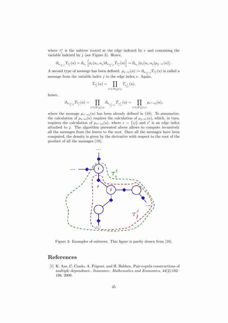
where τej is the subtree rooted at the edge indexed by e and containing thevariable indexed by j (see Figure 3). Hence,

∂uτie\iTτ ie(u) = ∂uj

[φe(ui, uj)∂uτe

j\jTτej (u)

]= ∂uj [φe(ui, uj)µj→e(u)] .

A second type of message has been defined: µj→e(u) := ∂uτej\jTτej (u) is called a

message from the variable index j to the edge index e. Again,

Tτej (u) =∏

e′∈N(j)\eTτj

e′(u),

hence,

∂uτej\jTτej (u) =

∏

e′∈N(j)\e∂u

τje′ \j

Tτje′

(u) =∏

e′∈N(j)\eµe′→j(u),

where the message µe′→j(u) has been already defined in (18). To summarize,the calculation of µe→i(u) requires the calculation of µj→e(u), which, in turn,requires the calculation of µe′→j(u), where e = {ij} and e′ is an edge indexattached to j. The algorithm presented above allows to compute recursivelyall the messages from the leaves to the root. Once all the messages have beencomputed, the density is given by the derivative with respect to the root of theproduct of all the messages (18).

Figure 3: Examples of subtrees. This figure is partly drawn from [10].

References

[1] K. Aas, C. Czado, A. Frigessi, and H. Bakken. Pair-copula constructions ofmultiple dependence. Insurance: Mathematics and Economics, 44(2):182–198, 2009.

45

[2] L.B.G Andersen and V.V. Piterbarg. Interest Rate Modeling. AtlanticFinancial Press, 2010.

[3] S. Demarta and A. J. McNeil. The t copula and related copulas. Interna-tional Statistical Review, 73(1):111–129, 2005.

[4] F. Durante and G. Salvadori. On the construction of multivariate extremevalue models via copulas. Environmetrics, 21(2):143–161, 2010.

[5] G. Frahm, M. Junker, and A. Szimayer. Elliptical copulas: applicabilityand limitations. Statistics & Probability Letters, 63(3):275–286, 2003.

[6] C. Genest, K. Ghoudi, and L-P. Rivest. Understanding relationships usingcopulas. North American Actuarial Journal, 2(3):143–149, 1998.

[7] C. Genest and B. Remillard. Test of independence and randomness basedon the empirical copula process. Test, 13(2):335–369, 2004.

[8] G. Gudendorf and J. Segers. Extreme-value copulas. In Copula Theory andIts Applications, page 127–145. Springer, 2010.

[9] M. Hofert, M. Machler, and A. J. McNeil. Archimedean copulas in highdimensions: Estimators and numerical challenges motivated by financialapplications. Journal de la Societe Francaise de Statistique, 154(1):25–63,2012.

[10] J. C. Huang. Cumulative distribution networks: Inference, estimation andapplications of graphical models for cumulative distribution functions. PhDthesis, University of Toronto, 2009.

[11] J.C. Huang and N. Jojic. Maximum-likelihood learning of cumulative distri-bution functions on graphs. Journal of Machine Learning Research W&CPSeries, 9:342–349, 2010.

[12] H. Joe. Multivariate models and dependence concepts. Chapman &Hall/CRC, 2001.

[13] D. Kim and J.M. Kim. Analysis of directional dependence using asymmetriccopula-based regression models. Journal of Statistical Computation andSimulation, 84(9):1990–2010, 2014.

[14] E. Liebscher. Construction of asymmetric multivariate copulas. Journal ofMultivariate Analysis, 99(10):2234–2250, 2008.

[15] B. G. Lindsay. Composite likelihood methods. Contemporary Mathematics,80(1):221–39, 1988.

[16] R.B. Nelsen. An introduction to copulas. Springer, 2006.

[17] M. Sklar. Fonctions de repartition a n dimensions et leurs marges. Publi-cations de l’Institut de Statistique de l’Universite de Paris, 8:229-231, 1959.

[18] T. Van Pham and G. Mazo. PBC: product of bivariate copulas.http://cran.r-project.org, 2014. R package version 1.2.

[19] L. Zhang and V. P. Singh. Gumbel–Hougaard copula for trivariate rainfallfrequency analysis. Journal of Hydrologic Engineering, 12(4):409–419, 2007.

46

Chapitre 5

Estimation de copulesmultivariées par la méthodedes moindres carrés pondérésbasée sur les coefficients dedépendance

Supposons que l’on dispose d’un échantillon d’une fonction de répartitionF d-variée (d > 2) dont la copule appartient à une famille indexée par unvecteur de paramètres θ et que l’on souhaite estimer ces paramètres. Supposonsaussi que cette copule n’admette pas de dérivées partielles sur son ensemble dedéfinition et que par conséquent, comme nous l’avions fait remarquer dans lapartie 3.1.2, il n’est pas possible de s’assurer des propriétés asymptotiques desméthodes bien connues de la littérature. Certaines de ces copules ont déjà étéprésentées dans la partie 1.3.2. D’autres ont été utilisées dans la pratique avecsuccès [20, 77]. Enfin, et surtout, c’est le cas de la classe de copules construitedans le chapitre 6.

Dans ce chapitre, pour estimer le paramètre θ, nous reconsidérons l’estima-teur des moindres carrés pondérés basé sur les coefficients de dépendances (3.8)de la partie 3.1.2 et établissons ses propriétés asymptotiques sans supposer queles copules admettent des dérivées partielles. Rappelons que l’estimateur estobtenu en minimisant la fonction

l(θ) =(D −D(θ)

)TW(D −D(θ)

), (5.1)

où D(θ) = (D1,2(θ), . . . ,Dd−1,d(θ)), D = (D1,2, . . . , Dd−1,d) et W est une ma-trice de poids ; Di,j(θ) est le coefficient de dépendance entre la i-ème et laj-ème variable d’intérêt sous le modèle, et Di,j est une estimation empirique dece coefficient. Par exemple, pour Di,j(θ), on peut prendre le coefficient rho deSpearman (1.5), et pour Di,j , on prendrait bien sûr sa version empirique (3.5).Les résultats sont obtenus sous des conditions naturelles d’identifiabilité desmodèles. Nous entendons par là que l’ensemble des coefficients de dépendance

47

des paires détermine la copule à l’intérieur d’une famille donnée. En particulier,l’application

θ 7→ (D1,2(θ), . . . ,Dd−1,d(θ))

devra être bijective, continue, et son inverse continue également. Les résultatsthéoriques sont illustrés sur des simulations et des données hydrologiques, oùnous estimons des copules possèdant une composante singulière. L’article pré-senté ci-dessous a été soumis pour publication, et est disponible à l’adressehttp://hal.archives-ouvertes.fr/hal-00979151.

48

Weighted least-squares inference for multivariate

copulas based on dependence coefficients

Gildas Mazo, Stephane Girard and Florence Forbes

Inria Grenoble Rhone-Alpes & Laboratoire Jean Kuntzmann,France

Abstract

In this paper, we address the issue of estimating the parameters ofgeneral multivariate copulas, that is, copulas whose partial derivativesmay not exist. To this aim, we consider a weighted least-squares esti-mator based on dependence coefficients, and establish its consistency andasymptotic normality. The estimator’s performance on finite samples isillustrated on simulations and a real dataset.

Keywords: partial derivatives, singular component, weighted least-squares,method-of-moments, dependence coefficients, parametric inference, multivariatecopulas.

1 Introduction

The concept of copulas is useful to model multivariate distributions. Given amultivariate random vector of interest, copulas allow to separate the analysisof the margins from the dependence structure. Standard books covering thissubject include [9, 24,29]. See also [13] for an introduction to this topic.

Some copulas possess a singular component, meaning that they are not ab-solutely continuous (with respect to the Lebesgue measure). For instance, letus consider the copula given below, introduced in [8]:

C(u1, u2, u3, u4) =

4∏

i=1

u1−∑j 6=i θiji

∏

i<j

min(ui, uj)θij , (1)

∑

j 6=iθij ≤ 1, i = 1, . . . , 4, θij = θji ∈ [0, 1].

One can see that, on the diagonal of the unit hypercube, the partial derivativesdo not exist. Yet, most inference methods for multivariate copulas make the as-sumption that these derivatives exist, and even are continuous. This is the case,for example, for the minimum-distance estimator [35], the simulated method ofmoments [31], and, of course, likelihood-based methods (Section 10.1 [24], [14]).When this assumption is not made, some methods can still be applied but onlyin specific situations. For example, when there are only two dimensions, onecan rely on the inversion of the Kendall’s tau, see [18] and [13]. When thereis an arbitrary number of dimensions but only one parameter to estimate, an

49

extension of this method can also be found in [15]. Also, if the copulas of inter-est are elliptical copulas, one can use the analysis of covariance structures [25].The issue that the partial derivatives need to exist and be continuous on theunit hypercube in order to properly apply most inference methods was alsoraised in [3, 34]. In these papers, the authors show how to weaken the classicaldifferentiability assumptions in the empirical copula process theory.

In order to estimate the parameters of general multivariate copulas, we con-sider a weighted least-squares (WLS) estimator based on dependence coeffi-cients. The consistency and asymptotic normality of the estimator are derivedwithout assuming that the copulas of interest have partial derivatives at all.This method is therefore broadly applicable and allows to estimate the param-eters of any kind of copulas, provided that one can calculate their dependencecoefficients.

In Section 2 of this paper, the consistency and asymptotic normality ofthe WLS estimator are established. The theoretical results are illustrated onsimulated and real datasets in Section 3. The proofs are postponed to theAppendix.

2 Asymptotic properties of the WLS estimatorbased on dependence coefficients

We derive the consistency and asymptotic normality of a generic WLS estima-tor in Section 2.1 and give three examples based on the Spearman’s rho, theKendall’s tau, and the extremal dependence coefficients in Section 2.2.

Let X(1), . . . ,X(n) with X(k) = (X(k)1 , . . . , X

(k)d ), k = 1, . . . , n, be inde-

pendent and identically distributed copies of a vector X = (X1, . . . , Xd) withdistribution F and copula C. The marginal distributions F1, . . . , Fd are as-sumed to be continuous. The copula C is assumed to belong to the family(Cθ) for θ ∈ Θ ⊂ Rq. The true parameter vector is denoted by θ0, that is,C = Cθ0 . Let p = d(d − 1)/2 be the number of variable pairs (Xi, Xj), fori = 1, . . . , d− 1, j = 2, . . . , d, i < j. Let us define the vector map

D : Θ→ D(Θ) ⊂ Rp (2)

θ 7→ (D1,2(θ), . . . ,Dd−1,d(θ)) ,

where Di,j(·) can represent, but is not limited to, a well chosen dependencecoefficient between the variables Xi and Xj (see Section 2.2 for examples).The space D(Θ) stands for the image of Θ by the multivariate map D. Thecoordinates of D(θ) are the Di,j(θ) sorted in the lexicographic order. When themap D is differentiable, its Jacobian matrix at θ = (θ1, . . . , θq) is denoted by

D(θ) =

∂D1,2(θ)∂θ1

∂D1,2(θ)∂θ2

· · · ∂D1,2(θ)∂θq

......

∂Dd−1,d(θ)∂θ1

∂Dd−1,d(θ)∂θ2

· · · ∂Dd−1,d(θ)∂θq

.

Besides, let D = (D1,2, . . . , Dd−1,d) be an empirical (nonparametric) estimator

of D(θ0). To simplify the notations, we shall write D(θ0) = D, Di,j(θ0) = Di,j

50

and D = D(θ0). Vectors are assumed to be column vectors and T denotes thetranspose operator.

The WLS estimator of θ0 studied in this paper is defined as

θ := arg minθ∈Θ

(D −D(θ)

)TW(D −D(θ)

), (3)

where W = Wn is a sequence (n = 1, 2, . . . ) of symmetric and positive definite

matrices with full rank. Let us denote ˆ(θ) the loss function to be minimized

in (3). In general, the minimizer θ of ˆ(·) may not exist, or may not be unique.However, it will be seen in Section 2.1 that the existence and uniqueness of θ

hold with probability tending to one as the sample size increases. Since W ispositive definite, the loss function ˆ is such that ˆ(θ) ≥ 0 for all θ ∈ Θ and

vanishes at θ if and only if θ ∈ D−1({D}), where D−1({D}) denotes the set

of all θ in Θ such that D(θ) = D. In this case, the WLS estimator does not

depend on the weights and D(θ) = D. Moreover, if the multivariate map D is

one-to-one, then the WLS estimator takes the form θ = D−1(D).

2.1 Asymptotic properties of the generic WLS estimator

The assumptions needed to derive the asymptotic properties of the WLS esti-mator are given below. The symbol ‖ · ‖ denotes the Euclidean norm.

Assumptions. (A1) The true parameter vector θ0 lies in the interior of Θ.Moreover, there exists ε0 > 0 such that the set {θ ∈ Θ : ‖θ− θ0‖ ≤ ε0} isclosed (and thus compact) in Rq.

(A2) As n→∞, the sequence of weight matrices W converges in probability toa symmetric and positive definite matrix W with full rank.

(A3) The map D defined in (2) is a twice continuously differentiable homeo-morphism such that D is of full rank.

(A4) As n→∞, the empirical estimator D is such that

D P→ D, and,√n(D −D

)d→ Np(0,Σ),

where Σ is some symmetric, positive definite p×p matrix noted as follows

Σ =

Σ1,2;1,2 Σ1,2;1,3 . . . Σ1,2;d−1,d

Σ1,3;1,2 Σ1,3;1,3 . . . Σ1,3;d−1,d

......

......

Σd−1,d;1,2 Σd−1,d;1,3 . . . Σd−1,d;d−1,d

. (4)

Assumption (A1), which is rather standard, see, e.g. [10], is not too restric-tive for most copula models. Indeed, a parameter lying in the parameter spaceboundaries often means that the copula of interest is in fact the independencecopula or one of the Frechet-Hoeffding bounds, that is, a copula where thedependence is “perfect”, see for instance [29] chapter 2. This is not an issue

51

because one does not encounter perfect dependence in practice. As for indepen-dence, one might carry out a statistical test as in [16], and, based on the results,decide whether independence holds or not. If not, then one can safely assumethat the parameters lie in the interior of the parameter space.

A sequence of weight matrices verifying Assumption (A2) can always be

constructed. A trivial example is W = Ip, where Ip is the identity matrix ofsize p. The construction of optimal weights is addressed in Proposition 1 below.

The estimation of the copula parameter vector is performed by matching thetheoretical and empirical dependence coefficients. Hence, a successful matchshould ensure that the resulting parameter vector estimate is close to the truevalue. This identifiability condition, also made in [10] in order to estimateextreme-value copulas with a singular component, is the essence of Assump-tion (A3). Assumption (A3) is hard to check in practice, except maybe forparticular simple cases when p = q, as in Section 3.2. Nonetheless, one canalways test the estimation procedure on simulated data, by, for instance, com-paring the expected asymptotic distribution to its estimated counterpart; seeSection 3.1 for an example of how to proceed.

The last assumption, (A4), naturally states that one should have convergenceof the dependence coefficient empirical estimator to ensure convergence of theWLS estimator.

Theorem 1. Assume that (A1)–(A4) hold. Then, as n → ∞ and with prob-ability tending to one, the WLS estimator defined by (3) exists and is unique.Moreover, it is consistent and asymptotically normal:

√n(θ − θ0)

d→ Nq (0,Ξ) , where (5)

Ξ =(DT

WD)−1

DTWΣWD

(DT

WD)−1

.

As usual, the results of Theorem 1 allow to derive the asymptotic distributionof quadratic forms in θ and D(θ). These asymptotics serve to build confidenceregions and statistical tests for the parameters and the dependence coefficients.Let χ2

q denote the Chi square distribution with q degrees of freedom. Let uswrite Ξ = Ξ(θ) and Σ = Σ(θ) to emphasize that in general these matricesdepend on θ. The continuity of matrices with respect to the parameter vector θis meant elementwise. Corollary 1, given below, may serve to build confidenceregions around θ or D(θ).

Corollary 1. Suppose that the assumptions of Theorem 1 hold.

(i) If Ξ(θ) is invertible for all θ in Θ and Σ(·) is continuous at θ0, then, asn→∞,

n(θ − θ0)TΞ(θ)−1(θ − θ0)d→ χ2

q.

(ii) Define Σ such that Σ is invertible and converges to Σ(θ0) in probabilityas n→∞. Then as n→∞,

n(D −D(θ0))T Σ−1

(D −D(θ0))d→ χ2

p.

52

For a particular value θ?1 ∈ Rr, r ≤ q − 1, the test H0 : θ01 = θ?1 againstH1 : θ01 6= θ?1, where θ0 = (θ01,θ02) ∈ Rr × Rq−r, may be carried out usingthe asymptotic approximation suggested by Corollary 2, given next. In general,write θ = (θ1,θ2) ∈ Rr × Rq−r for θ ∈ Θ, and, likewise, θ = (θ1, θ2). LetΞ1(θ1,θ2) denote the r × r asymptotic covariance matrix corresponding to θ1,that is, the upper left part of Ξ(θ1,θ2).

Corollary 2. Under the assumptions of Corollary 1 (i), as n→∞,

n(θ1 − θ?1)TΞ1(θ?1, θ2)−1(θ1 − θ?1)d→ χ2

r.

The test H0: “the chosen parametric model is the true model of the under-lying copula” against H1 “the chosen parametric model is false” may be carriedout by using the asymptotic approximation suggested by Corollary 3 below,adapted from [22].

Corollary 3. Suppose that the assumptions of Theorem 1 and Corollary 1 (ii)hold. For θ ∈ Θ, define

A(θ) := D(θ)(D(θ)T D(θ)

)−1

D(θ)T ,

A = A(θ), and denote by k the rank of Ip−A(θ0). If Σ(θ) is invertible for allθ in Θ and Σ(·) is continuous at θ0, then as n→∞,

n(D(θ)− D

)T(Ip − A)[(Ip − A)Σ(Ip − A) + A]−1(Ip − A)

(D(θ)− D

)→ χ2

k.

The asymptotic covariance matrix Ξ in (5) depends on the weight matrixW. The optimal weight matrix W?, in the sense that it allows to minimize theasymptotic covariance matrix Ξ, is given in Proposition 1 below (due to [22]).The above mentioned ordering of covariance matrices is to be understood in thefollowing sense. The notation A ≥ 0 means that the matrix A is nonnegativedefinite. For two nonnegative definite matrices A and B, define A to be lessor equal than B if B − A ≥ 0. It is easily checked that A ≤ B impliestr(A) ≤ tr(B), where tr(·) stands for the trace operator of matrices. Thus,the distribution with the smallest covariance matrix is the one for which thesum of the variances is minimum. In view of (6), an optimal estimator, that is,an estimator that leads to the smallest asymptotic covariance matrix, can beconstructed by letting the sequence of weight matrices converge to Σ−1.

Proposition 1. Suppose that Σ defined in (A4) is invertible. Then the asymp-totic covariance matrix Ξ is minimum for W? such that

W?D ∝ Σ−1D, (6)

where the symbol ∝ denotes proportionality.

An estimate of the optimal weight matrix Σ−1 can be based on empirical

data or constructed as follows. Define the zero-step estimator θ0

to be the

WLS estimator (3) with W = Ip. Define the one-step estimator θ1

to be the

WLS estimator with W = Σ−1(θ0), where Σ(θ

0) is an estimate of Σ based

on the zero-step estimator. For instance, one may simulate data according

53

to C = C(θ0) and use them to construct Σ(θ

0). This one-step estimator is

then an optimal estimator. The performances of the zero-step and the optimalestimators will be compared in Section 3.1.

When there are as many pairs as parameters, the WLS estimator does notdepend on the weights, as stated in the next proposition.

Proposition 2. Suppose that the assumptions of Theorem 1 hold. If p = qthen, as n→∞ and with probability tending to one,

θ = D−1(D), (7)

and

√n(θ − θ0)

d→ Nq

(0,(DT D

)−1

DTΣD

(DT D

)−1). (8)

2.2 Examples of three dependence coefficients verifyingAssumption (A4)

Three examples of a dependence coefficient for which the pair of vectors (D, D)satisfies Assumption (A4) are provided. These coefficients are the Spearman’srho, the Kendall’s tau, and the extremal dependence coefficient. They are widelyused in practice, and that is why we illustrate our methodology on them. Butothers can be used, as long as (A4) holds. See [24,29] for more about these coeffi-cients and [23] for their asymptotic properties. Recall that Fi is the distributionof Xi and let

Fi(x) =1

n+ 1

n∑

k=1

1(X(k)i ≤ x), x ∈ R.

Put Ui = Fi(Xi) and U(k)i = Fi(X

(k)i ). Recall that Fi,j is the distribution

function of (Xi, Xj) and that Ci,j denotes its copula.

Example 1 (Spearman’s rho). The Spearman’s rho dependence coefficient ofthe pair (Xi, Xj) is given by

Di,j = 12

∫

[0,1]2Ci,j(u, v) du dv − 3. (9)

Its empirical counterpart is defined as

Di,j =

∑nk=1

(U

(k)i − U i

)(U

(k)j − U j

)

[∑nk=1

(U

(k)i − U i

)2∑nk=1

(U

(k)j − U j

)2]1/2

,

where Ui =∑nk=1 U

(k)i /n. This empirical estimator is a U-statistic [23], whose

theory is well known, see, e.g. [36] Chapter 12. In particular, it has been estab-lished in [23] Section 9 that Assumption (A4) holds with

Σi,j;k,l = 9

∫

[0,1]2[(1− 2ui)(1− 2uj)− 2ui − 2uj + 4Ii(uj) + 4Ij(ui)− ρij ]

× [(1− 2uk)(1− 2ul)− 2uk − 2ul + 4Ik(ul) + 4Il(uk)− ρkl] dC(u1, . . . , ud),

54

where Ij(u) =∫ 1

0Cij(u, v)dv and Ii(v) =

∫ 1

0Cij(u, v)du. Let us note that this

result holds without any condition on the underlying copula.

Example 2 (Kendall’s tau). The Kendall’s tau dependence coefficient of thepair (Xi, Xj) is given by

Di,j = 4

∫

[0,1]2Ci,j(u, v) dCi,j(u, v)− 1. (10)

Its empirical counterpart is defined as

Di,j =

(n

2

)−1∑

k<l

sign(

(X(k)i −X(l)

i )(X(k)j −X(l)

j )), (11)

where sign(x) = 1 if x > 0, −1 if x < 0 and 0 if x = 0. This empirical estimatoris also a U-statistic and the same discussion as in Example 1 also yields thatAssumption (A4) holds with

Σi,j;k,l = 4

∫

[0,1]2[4Ci,j(ui, uj) + 1−Di,j − 2ui − 2uj ] (12)

× [4Ck,l(uk, ul) + 1−Dk,l − 2uk − 2ul] dC(u1, . . . , ud).

Again, let us note that this result holds without any condition on the underlyingcopula.

The third example deals with extreme-value copulas, which are theoreticallywell grounded for performing a statistical analysis of extreme values, such asmaxima of samples. Recall that a copula C# is an extreme-value copula if there

exists a copula C such that

C#(u1, . . . , ud) = limm↑∞

Cm(u1/m1 , . . . , u

1/md ), (u1, . . . , ud) ∈ [0, 1]d,

see, e.g. [20]. The class of extreme-value copulas corresponds exactly to theclass of max-stable copulas, that is, the copulas C# such that

Cm# (u1/m1 , . . . , u

1/md ) = C#(u1, . . . , ud), m ≥ 1, (u1, . . . , ud) ∈ [0, 1]d.

The extremal dependence coefficient is implicitely defined by the following rep-resentation of bivariate extreme-value copulas on the diagonal of the unit square:

C#(u, u) = u2−λ, λ ∈ [0, 1]. (13)

If λ = 0 then C#(u, u) = Π(u, u) = u2, where Π stands for the independencecopula. If λ = 1 then C#(u, u) = M(u, u) = min(u, u) = u, where M standsfor the Frechet-Hoeffding upper bound for copulas, that is, the case of perfectdependence. In the case of extreme-value copulas, the extremal dependencecoefficient corresponds to the well known upper tail dependence coefficient

λ = limu↑1

1− 2u+ C#(u, u)

1− u ,

which measures the dependence in the tails. Nonetheless, for extreme-value cop-ulas, the interpolation between Π and M on the diagonal of the unit square (13)

55

makes the extremal dependence coefficient a natural coefficient of general de-pendence, and not just a coefficient that measures dependence in the tails. Forfurther information about extreme-value statistics, see, e.g. [5]. An accountabout extreme-value copulas can be found in [20].

Estimators of the extremal dependence coefficient for which the asymptoticproperties are derived under unknown margins can be found in [2, 19]. How-ever, in order to obtain the results, the existence of partial derivatives for theunderlying copulas was assumed. Hence, these estimators cannot be used sincewe aim at estimating the parameters of copulas for which these derivatives maynot exist.

If the marginal distributions are assumed to be known, however, various es-timators of the extremal dependence coefficient and their asymptotic propertiescan be found in the literature [4,7,11,21,32]. A review can be found in [20]. Ourchoice of the estimator presented in Example 3 below, that of [11], is arbitrary.One can choose an other estimator in the literature and adapt the results.

Example 3 (Extremal dependence coefficient). Assume that the copula of in-terest C is an extreme-value copula and let Di,j be the extremal dependencecoefficient of the pair (Xi, Xj), implicitely defined in (13), and given by

Di,j = 2 + logCi,j(e−1, e−1). (14)

Its empirical counterpart, as defined in [11], is given by

Di,j = 3− 1

1−∑nk=1 max(U

(k)i , U

(k)j )/n

.

By adapting [11] to the multivariate case, Assumption (A4) holds with

Σi,j;k,l = (3−Di,j)2(3−Dk,l)2 Cov (max(Ui, Uj),max(Uk, Ul)) . (15)

In practice, the margins are usually unknown . However, assuming that Fis an extreme-value distribution, the margins should be Generalized Extreme-Value (GEV) distributions, see [5]. Therefore, to estimate the parameters ofthe GEV, one can apply a method known as “inference functions for margins”(IFM, see [24] Section 10) whose asymptotic properties are well established.

3 Illustrations on simulated and real datasets

In order to assess the WLS estimator’s performance on finite samples, numericalexperiments are undertaken in Section 3.1 and a real dataset application ispresented in Section 3.2. In both the experiments and the application, weaim at estimating the parameters of multivariate copulas possessing a singularcomponent.

3.1 Estimating the parameters of multivariate copulas pos-sessing a singular component

By substituting the Frechet copulas [12]

C0k(u0, uk) = θk min(u0, uk) + (1− θk)u0uk, θk ∈ [0, 1]

56

into the one-factor copula [27]

C(u1, . . . , ud) =

∫ 1

0

d∏

k=1

∂C0k(u0, uk)

∂u0du0,

one obtains a copula C with a singular component and whose bivariate marginsare given by the following Frechet copulas

Cij(ui, uj) = θiθj min(ui, uj) + (1− θiθj)uiuj , θi, θj ∈ [0, 1]. (16)

The Spearman’s rho and Kendall’s tau coefficients of (16) are respectively equalto θiθj and θiθj(θiθj + 2)/3. The extreme-value copula C# associated to C canbe derived by calculating the limit

C#(u1, . . . , ud) = limn↑∞

Cn(u1/n1 , . . . , u

1/nd ).

It appears that the bivariate margins of C# are Cuadras-Auge copulas [6]

C#,ij(ui, uj) = min(ui, uj) max(ui, uj)1−θiθj , θi, θj ∈ [0, 1]

with extremal dependence coefficient given by θiθj . Similarly to C, C# possessesa singular component.

d = 4 d = 10zero-step one-step zero-step one-step

(S1) 0.11 0.11 0.10 0.12n = 50 (S2) 0.10 0.10 0.09 0.10

(S3) 0.18 0.18 0.17 0.20(S1) 0.06 0.06 0.05 0.05

n = 200 (S2) 0.05 0.05 0.04 0.04(S3) 0.10 0.10 0.09 0.09(S1) 0.04 0.04 0.03 0.03

n = 500 (S2) 0.03 0.03 0.03 0.03(S3) 0.06 0.06 0.06 0.05

Table 1: MAEs for the three studied situations with respect to the data samplesize n and dimension d. The results are averaged over 200 replications.

The two copulas C and C# are considered in the following numerical ex-periment. For each combination (d, n) with d = 4, 10 and n = 50, 200, 500, wegenerated 200 datasets according to these copulas. The true parameter vectorcoordinates θ0k, k = 1, . . . , d, were chosen to be regularly spaced between 0.3and 0.9. Three situations were studied:

(S1) the parameters of C are estimated with the Spearman’s rho (see Exam-ple 1),

(S2) the parameters of C are estimated with the Kendall’s tau (see Example 2),and

(S3) the parameters of C# are estimated with the extremal dependence coeffi-cient (see Example 3).

57

In situation (S1), Assumption (A3) is verified, see [28]. For each situation (Si)above, the zero-step and one-step WLS estimators of Section 2.1 were tested(recall that the one-step estimator is optimal, see Proposition 1). For eachdataset and each situation (Si), the mean absolute error, defined as

MAE =1

d

d∑

k=1

|θk − θ0k|

was computed and averaged over the 200 replications. These criteria are re-ported in Table 1. It appears from this Table that there is almost no differencebetween the zero-step and one-step estimators. This lack of weighting effectwas also mentioned in [31] Section 3. This suggests that the zero-step esti-mator is already near optimal. The comparison of the rows (S1) and (S2)shows that the choice between the Spearman’s rho and Kendall’s tau in theWLS estimator has very little impact on its performance. Estimating the pa-rameters of an extreme-value copula with the extremal dependence coefficient,however, appears to be less accurate–see the (S3) row of the table. Finally, thecomparison of the two columns d = 4 and d = 50 shows that the dimensionof the inference problem does not seem to affect the estimator’s performance.This property makes it very attractive to deal with high-dimensional applica-tions. To complete the study of the estimator’s abilities, its asymptotic distri-bution derived in Theorem 1 is tested. Since this distribution is multivariate,we checked the Chi-square approximation of Corollary 1 instead. The values

n(θ(r) − θ0)TΞ(θ

(r))−1(θ

(r) − θ0), r = 1, . . . , 200, should be approximately χ2d

distributed (here the dimension is equal to the number of parameters), where

θ(r)

denotes the parameter vector estimated on the r-th dataset replication.This approximation, shown in Figure 1, seems rather satisfactory.

3.2 Measuring uncertainty for multivariate return periodsin hydrology

In hydrology, the severity and frequency of extreme events must be quantified.Such potentially dangerous events are underlain by the behavior of a randomvector (X1, . . . , Xd) distributed according to a certain distribution F with con-tinuous margins F1, . . . , Fd and copula C. Suppose that C is determined by aparameter vector θ in Θ. For a certain potentially dangerous event, define thereturn period T and the critical level p through the relationship

T =1

1−Kθ(p), (17)

where Kθ(t) = P (C(F1(X1), . . . , Fd(Xd)) ≤ t), t ∈ [0, 1], is called the Kendall’sdistribution function associated to C, see [30]. The return period can be inter-preted as the average time elapsing between two dangerous events. For instance,T = 30 years means that the event happens once every 30 years in average. Thecritical level can be viewed as a measure of how dangerous the underlying eventis. The following question naturally arises: given a certain return period, whatis the critical level of the underlying event? To answer this question, it sufficesto invert (17) to get p as a function of T :

pT (θ) = K−1θ (1− 1/T ).

58

Figure 1: Histograms of n(θ(r) − θ0)TΞ(θ

(r))−1(θ

(r) − θ0), r = 1, . . . , 200 to-gether with the density of a χ2

d distribution. The considered experiment param-eters were n = 500 and d = 4. Upper left: (S2). Upper right: (S1). Bottom:(S3).

Let θ0 denote the true parameter vector and let pT = pT (θ0). The estimationof pT , or, in other words, the estimation of θ0, was performed in [8] for all thepairs of d = 3 sites in Italy (Airole, Merelli and Poggi). The parametric modelproposed for C was the extreme-value copula

C(u1, . . . , ud) =

(d∏

i=1

u1−θii

)min

i=1,...,d(uθii ), θi ∈ [0, 1], i = 1, . . . , d. (18)

As it can be seen from (18), this copula has a singular component. The authorschose to base the inference on the Kendall’s tau (see Example 2). For θ in[0, 1]d, the Kendall’s tau coefficients are given by

τi,j(θ) =θiθj

θi + θj − θiθj, i < j. (19)

By inverting (19), one obtains

θi =1

2

(1 +

1

τ i,j+

1

τ i,k− 1

τ j,k

), (20)

59

where i, j, k denote the indexes of the three sites and τi,j is given by (11).Observe that this is the solution of the equation (7), and, under the light ofProposition 2 (since p = q = d = 3), we see that this estimator has the smallestasymptotic variance within the class (3). However, in [8], the asymptotic be-

havior of θ = (θ1, θ2, θ3) was not derived. This is done next, and we shall seethat it allows to quantify the uncertainties around the critical levels.

The asymptotic normality of√n(θ − θ0) is established by applying Theo-

rem 1. It suffices to verify that assumption (A3) holds, which is easily checkedfrom (19). Hence, as n→∞

√n(θ − θ0)

d→ N(0,Ξ), (21)

where Ξ is given by (8) and (12). Now, the derivation of the asymptotic behaviorof the critical levels is straightforward. From (21), we get by the delta-methodthat, as n→∞

√n(pT (θ)− pT

)d→ N(0, s2

T ), (22)

with s2T = pTΞpTT , and where pT is the Jacobian of pT (·) at the true parameter

value. It follows that confidence intervals can be computed from the finite-sample approximation of (22), provided that the sample size is large enough.In [8], the critical levels in terms of return periods were reported for the threepair of sites (Airole, Merelli), (Airole, Poggi) and (Merelli, Poggi). We addedto their figure 95% confidence intervals for the critical levels (Figure 2).

The test based on Corollary 3 has no power to detect a wrong model in thissituation. Indeed, since D(θ) = D, the test statistic is always zero. Other testscan be performed to achieve such a task, see the original paper [8].

When studying extreme events, it is common to have only a limited amountof data. For instance, in [8], only n = 34 (multivariate) observations wereavailable. With such a small sample size, the approximation of the distributionof√n(pT (θ) − pT ) to a normal distribution may be questionable. To assess

the goodness of this approximation for small and moderate sample sizes, wecarried out the following numerical experiment. N = 500 datasets of size n ∈{34, 100} were generated according to (18) with θ0 = (0.6, 0.7, 0.2). For the m-

th dataset (m = 1, . . . , N), the parameter vector estimate θ(m)

was computed.

Let sT (θ(m)

) be the asymptotic standard deviation in (22) at θ(m)

where sT (θ)

is regarded as a function of θ. The critical levels pT (θ(m)

) together with the 95%

confidence bands pT (θ(m)

)±1.96sT (θ(m)

)/√n were computed for T = 10, 20, 30.

Some of the θ(m)

did not lie in their theoretical bounds [0, 1], which led to

numerical difficulties for computing sT (θ(m)

). Therefore, these were droppedfrom the experiment. The results reported Table 2 show that the finite sampleapproximation is rather good for n = 100. Even for n = 34, this approximationappears to be good for the pair Airole-Merelli. Despite these encouraging resultsfor moderate and small samples, we finish by stressing that the number of

missing outputs (recall that this happens when θ(m)

do not belong to [0, 1])were quite high: 354 and 298 over the 500 dataset replications for n = 34 andn = 100 respectively. Consequently, it would be of interest to improve theestimator (20) to reduce this vexing effect.

60

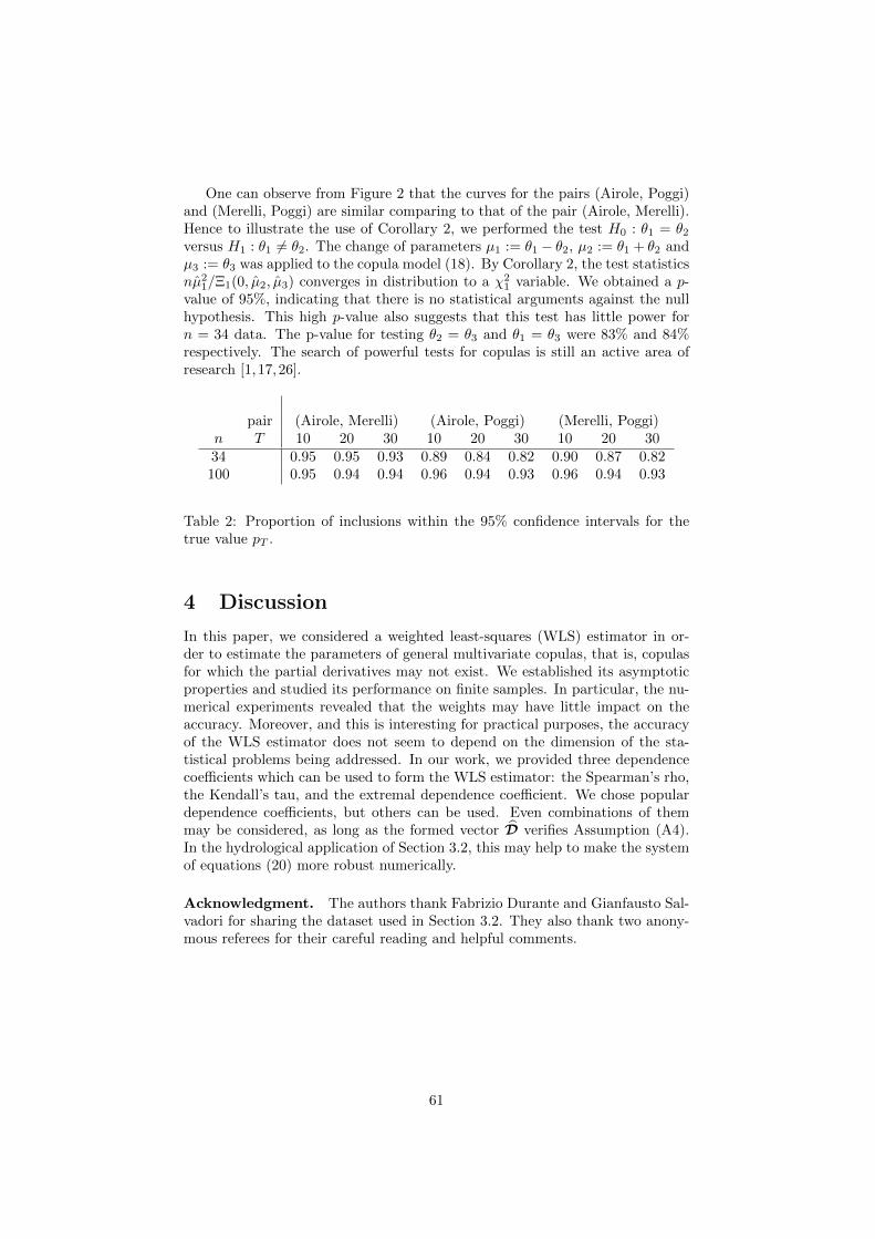
One can observe from Figure 2 that the curves for the pairs (Airole, Poggi)and (Merelli, Poggi) are similar comparing to that of the pair (Airole, Merelli).Hence to illustrate the use of Corollary 2, we performed the test H0 : θ1 = θ2

versus H1 : θ1 6= θ2. The change of parameters µ1 := θ1 − θ2, µ2 := θ1 + θ2 andµ3 := θ3 was applied to the copula model (18). By Corollary 2, the test statisticsnµ2

1/Ξ1(0, µ2, µ3) converges in distribution to a χ21 variable. We obtained a p-

value of 95%, indicating that there is no statistical arguments against the nullhypothesis. This high p-value also suggests that this test has little power forn = 34 data. The p-value for testing θ2 = θ3 and θ1 = θ3 were 83% and 84%respectively. The search of powerful tests for copulas is still an active area ofresearch [1, 17,26].

pair (Airole, Merelli) (Airole, Poggi) (Merelli, Poggi)n T 10 20 30 10 20 30 10 20 3034 0.95 0.95 0.93 0.89 0.84 0.82 0.90 0.87 0.82100 0.95 0.94 0.94 0.96 0.94 0.93 0.96 0.94 0.93

Table 2: Proportion of inclusions within the 95% confidence intervals for thetrue value pT .

4 Discussion

In this paper, we considered a weighted least-squares (WLS) estimator in or-der to estimate the parameters of general multivariate copulas, that is, copulasfor which the partial derivatives may not exist. We established its asymptoticproperties and studied its performance on finite samples. In particular, the nu-merical experiments revealed that the weights may have little impact on theaccuracy. Moreover, and this is interesting for practical purposes, the accuracyof the WLS estimator does not seem to depend on the dimension of the sta-tistical problems being addressed. In our work, we provided three dependencecoefficients which can be used to form the WLS estimator: the Spearman’s rho,the Kendall’s tau, and the extremal dependence coefficient. We chose populardependence coefficients, but others can be used. Even combinations of themmay be considered, as long as the formed vector D verifies Assumption (A4).In the hydrological application of Section 3.2, this may help to make the systemof equations (20) more robust numerically.

Acknowledgment. The authors thank Fabrizio Durante and Gianfausto Sal-vadori for sharing the dataset used in Section 3.2. They also thank two anony-mous referees for their careful reading and helpful comments.

61

Figure 2: Critical levels pT (θ) for T = 2, . . . , 40 together with 95% confidenceintervals.

62

Appendix: proofs

In order to prove Theorem 1, we first establish two lemmas. These lemmas, aswell as their proofs, are adapted from [10]. It will appear that the proof of thetheorem is a straightforward application of these lemmas.

Let Θ and ε0 be defined as in assumption (A1). Define the vector map

ϕ : Θ ⊂ Rq → ϕ(Θ) ⊂ Rp (23)

ϕ(θ) 7→ (ϕ1(θ), . . . , ϕp(θ))T ,

and assume that ϕ is twice continuously differentiable. Denote by ϕ(θ) thep× q Jacobian matrix of ϕ at θ and define ϕ := ϕ(θ0). Let

Yn = (Yn,1, . . . , Yn,p)T

be a random vector in Rp depending on an integer n and assume that YnP→

ϕ(θ0) as n→∞. Let W = Wn be a p×p symmetric and positive definite matrix

with full rank and suppose that W converges in probability to a symmetricand positive definite matrix W with full rank as n → ∞. Then the Cholesky

decomposition entails that W = VT V for some p× p matrix V. Denote by Θn

the set of all minimizers of the loss function

`n(θ) = (Yn −ϕ(θ))T

W (Yn −ϕ(θ)) (24)

=∥∥∥V (Yn −ϕ(θ))

∥∥∥2

, θ ∈ Θ,

where ‖ · ‖ stands for the Euclidean norm. Observe that this set may containseveral or no elements. Let Hn(θ) be the Hessian matrix of `n at θ, that is, thematrix whose (k, l) element is given by

Hn,kl(θ) =∂2`n(θ)

∂θk∂θl.

Let Q(θ) be the q × q matrix whose (k, l) element writes

Qkl(θ) =

(∂2ϕ1(θ)

∂θk∂θl, . . . ,

∂2ϕp(θ)

∂θk∂θl

)WT (ϕ(θ)−ϕ(θ0)) ,

and H(θ) be the q × q matrix defined by

H(θ) = 2(Q(θ) + ϕ(θ)TWT ϕ(θ)

).

Finally write Bε(θ0) = {θ ∈ Θ : ||θ − θ0|| ≤ ε} the closed ball around θ0 withradius ε > 0 and assume that there exists ε0 > 0 such that Bε0(θ0) is closed.Then Bε(θ0) is compact for all 0 < ε ≤ ε0.

Lemma 1. (i) The elementwise convergence Hn(θ)P→ H(θ) holds uniformly

for all θ in Bε0(θ0).

(ii) If ϕ is of full rank then, with probability tending to 1, Hn(θ) is positivedefinite for all θ in some closed neighborhood of θ0.

63

Proof. (i) It is easily seen that Hn(θ) = 2(ϕ(θ)TWT ϕ(θ) + Qn(θ)

)where

Qn(θ) is a q × q matrix such that its (k, l) element is given by

Qn,kl(θ) =

(∂2ϕ1(θ)

∂θk∂θl, . . . ,

∂2ϕp(θ)

∂θk∂θl

)WT (ϕ(θ)−Yn) .

Let Wji denote the element of W in the j-th row and i-th column. For all θ inBε0(θ0),

1

2|Hn,kl(θ)−Hkl(θ)| ≤

p∑

i,j=1

∣∣∣∂ϕi(θ)

∂θk

∂ϕj(θ)

∂θl

∣∣∣∣∣∣Wij −Wij

∣∣∣

+

p∑

i,j=1

∣∣∣∂2ϕi(θ)

∂θk∂θl

∣∣∣∣∣∣Wij −Wij

∣∣∣∣∣ϕj(θ)− Yn,j

∣∣

+

p∑

i,j=1

∣∣∣∂2ϕi(θ)

∂θk∂θl

∣∣∣∣∣Wij

∣∣∣∣ϕj(θ0)− Yn,j∣∣.

Since ϕj and its first and second order derivatives are continuous on the closedand thus compact set Bε0(θ0), they are uniformly bounded by some constanton this set. Therefore, as n→∞,

supθ∈Bε0 (θ0)

|Hn,kl(θ)−Hkl(θ)| P→ 0,

which follows from the weak consistency of Yn and W.(ii) The matrix H(θ0) is positive definite. Hence its eigenvalues are posi-

tive. Since an eigenvalue is a continuous function of the parameter vector [33](Theorem 3.13), for each eigenvalue of H, there exists a neighborhood such thatif θ belongs to this neighborhood, then this eigenvalue at θ is positive. Hence,since there is only a finite number of eigenvalues, it follows that there exists aneighborhood Bδ(θ0) (δ > 0) on which H(θ) is positive definite.

Now define

Aij =

{sup

θ∈Bε0 (θ0)

|Hn,ij(θ)−Hij(θ)| ≤ infx∈Rq,x 6=0, θ∈Bδ(θ0)

xTH(θ)x

2∑qi,j=1 |xixj |

}

and put A =⋂i,j

Aij . On the event A, for all x 6= 0 and for all θ in Bε0(θ0), we

have

∣∣xT (H(θ)−Hn(θ)) x∣∣ ≤

q∑

i,j=1

|xixj | infx∈Rq,x 6=0, θ∈Bδ(θ0)

xTH(θ)x

2∑qi,j=1 |xixj |

≤ infθ∈Bδ(θ0)

xTH(θ)x

2.

If, moreover, θ ∈ Bδ(θ0), then

xTHn(θ)x ≥ xTH(θ)x

2> 0

64

because H(θ) is positive definite on Bδ(θ0). Hence on A and for all θ inBδ(θ0)

⋂Bε0(θ0), the matrix Hn(θ) is positive definite. By (i), P (A) → 1

as n→∞, which concludes the proof.

Lemma 2. (i) If ϕ in (23) is an homeomorphism, then for all ε such that0 < ε ≤ ε0, as n→∞,

P[Θn 6= ∅ and Θn ⊂ Bε(θ0)

]→ 1.

(ii) If, moreover, ϕ(θ0) is of full rank then as n→∞,

P[

card Θ = 1]→ 1,

where card denotes the cardinal of a set. Define θ to be the unique element

of Θ if card Θ = 1, and any arbitrary point otherwise. Then θP→ θ0 as

n→∞.

(iii) If in addition to the assumptions of (i) and (ii)

√n(Yn −ϕ(θ0))

d→ Np(0,Σ)

then

√n(θ − θ0)

d→ Nq

(0,(ϕTWϕ

)−1ϕTWΣWϕ

(ϕTWϕ

)−1)

Proof. (i) Let 0 < ε ≤ ε0. Since ϕ is a homeomorphism and W has

full rank, Vϕ is also an homeomorphism. Hence there exists δ > 0 such thatθ ∈ Θ and ‖V (ϕ(θ)−ϕ(θ0)) ‖ ≤ δ imply ‖θ − θ0‖ ≤ ε. Thus for every

θ ∈ Θ with ‖θ − θ0‖ > ε we have ‖V (ϕ(θ)−ϕ(θ0)) ‖ > δ. On the event

An = {‖V (ϕ(θ0)−Yn) ‖ ≤ δ/2} and for θ outside Bε(θ0), the inequality

‖V (ϕ(θ)−ϕ(θ0)) ‖ ≤ ‖V (ϕ(θ)−Yn) ‖+ ‖V (Yn −ϕ(θ0)) ‖

implies

‖V (ϕ(θ)−Yn) ‖ ≥ ‖V (ϕ(θ)−ϕ(θ0)) ‖ − ‖V (Yn −ϕ(θ0)) ‖> δ − δ/2= δ/2

≥ ‖V (Yn −ϕ(θ0)) ‖.

Therefore

minθ∈Bε(θ0)

‖V (Yn −ϕ(θ)) ‖ ≤ infθ/∈Bε(θ0)

‖V (Yn −ϕ(θ)) ‖,

where in the left hand side the minimum is attained because Bε(θ0) is compact.

By consistency of Yn and W, we have P (An) → 1. It follows that the event{Θn 6= ∅ and Θn ⊂ Bε(θ0)

}has probability tending to 1.

65

(ii) Without loss of generality denote by Bη(θ0), η < ε0, the closed neigh-borhood of Lemma 1 (ii). Assume that the event{

Θ 6= ∅, Θ ⊂ Bη(θ0) and Hn(θ) is positive definite for all θ in Bη(θ0)}

(25)

happens. Let θ ∈ Bη(θ0) and θ? be a vector in Θ. A Taylor expansion of `nin (24) at θ? gives

`n(θ) = `n(θ?) + (θ − θ?)TO`n(θ?) +1

2(θ − θ?)THn(θ)(θ − θ?),

where θ = tθ+ (1− t)θ?, t ∈ (0, 1) and O`n denotes the gradient of `n. In viewof Lemma 2 (i), θ? is in some open neighborhood of θ0 and thus O`n(θ?) = 0.The fact that θ ∈ Bη(θ0) entails that Hn(θ) is positive definite. Therefore,we have shown that `n(θ) > `n(θ?) for all θ in Bη(θ0). This implies that the

cardinal of Θ is 1 when (25) holds. By Lemma 1 (ii) and Lemma 2 (i), theevent (25) has probability tending to 1, hence, P [ card Θ = 1]→ 1. Now let θbe as in Lemma 2 (ii) and let ε > 0. Without loss of generality, assume thatε ≤ ε0. Then

limn→∞

P[θ ∈ Bε(θ0)

]= limn→∞

P[θ ∈ Bε(θ0) and card Θ = 1

]= 1,

the last equality holding because of Lemma 2 (i). Thus the consistency of θ isproved.

(iii) A Taylor expansion for the gradient O`n of `n in equation (24) aroundθ0 entails

O`n(θ) = O`n(θ0) + Hn(θ)(θ − θ0),

where θ = tθ + (1− t)θ0, t ∈ (0, 1). By the same arguments as in the proof ofLemma 2 (ii), O`n(θ) = 0, hence,

√nHn(θ)(θ − θ0) =

√n(O`n(θ)− O`n(θ0)

)

= −√nO`n(θ0)

= 2ϕTW√n (Yn −ϕ(θ0)) .

For x in Rq, we have

P[√

nHn(θ)(θ − θ0) ≤ x]

=P[√

nHn(θ)(θ − θ0) ≤ x and card Θ = 1]

+P[√

nHn(θ)(θ − θ0) ≤ x and card Θ 6= 1].

(26)

Since the second term in the sum in the right hand side of (26) tends to 0, wehave that

limn→∞

P[√

nHn(θ)(θ − θ0) ≤ x and card Θ = 1]

= limn→∞

P[√

nHn(θ)(θ − θ0) ≤ x]

= limn→∞

P[2ϕTW

√n (Yn −ϕ(θ0)) ≤ x

].

66

By the assumptions of Lemma 2 (iii) and by consistency of W, we have

2ϕTW√n (Yn −ϕ(θ0))

d→ Nq(0, 4ϕTWΣWT ϕ

).

If Hn(θ) converges in probability to H(θ0) = 2ϕWϕ, then

√n(θ − θ0)

d→ Nq

(0,(ϕTWT ϕ

)−1ϕTWΣWT ϕ

[(ϕTWT ϕ

)−1]T)

.

Therefore, to conclude the proof, it suffices to prove that Hn(θ)P→ H(θ0).

Let ε > 0. Assume that

supθ∈Bε0 (θ0)

|Hn,ij(θ)−Hij(θ)| < ε

2.

The map θ 7→ Hn,ij(θ) is continuous, hence, there exists δ > 0 such that

|θ− θ0| < δ implies |Hn,ij(θ)−Hn,ij(θ0)| < ε/2. Assume that θ ∈ Bδ(θ0) andsuppose without loss of generality that δ ≤ ε0. Then it holds that

|Hn,ij(θ)−Hij(θ0)| ≤ |Hn,ij(θ)−Hn,ij(θ0)|+ |Hn,ij(θ0)−Hij(θ0)|<ε

2+ε

2= ε.

By Lemma 1 (i) and Lemma 2 (i) we have shown that for all ε > 0, the event{|Hn,ij(θ)−Hij(θ0)| ≤ ε

}has probability tending to 1. Hence the proof is

finished.

Proof of Theorem 1

The proof of Theorem 1 is a direct application of Lemma 2 with ϕ = D andYn = D.

Proof of Corollary 1

(i) The limiting covariance matrix of θ, viewed as a function of θ is given by

Ξ(θ) =(D(θ)TWD(θ)

)−1

D(θ)TWΣ(θ)WD(θ)(D(θ)TWD(θ)

)−1

.

By assumption, D(·) and Σ(·) are continuous at θ0, hence so is Ξ(·). Therefore,since θ converges in probability to θ0, we also have that Ξ(θ) converges inprobability to Ξ(θ0). Moreover, since Ξ(θ) is invertible and nonnegative definite

for all θ in Θ, we have Ξ(θ) = Ξ1/2(θ)Ξ1/2(θ) where Ξ1/2(θ) is also invertible.Therefore, by Theorem 1, as n→∞,

√nΞ(θ)−1/2(θ − θ0)

d→ N(0, Iq),

leading to the desired result.(ii) By Assumption (A4),

√n(D −D(θ0)

)d→ Np(0,Σ(θ0))

as n → ∞. The arguments in the proof of (i) can be easily adapted to prove(ii).

67

Proof of Corollary 2

The proof of Corollary 2 is similar to that of Corollary 1 (i).

Proof of Corollary 3

Note D0 := D(θ0) and write

D(θ)− D = D(θ)−D0 + D0 − D. (27)

A Taylor expansion yields

D(θ)−D0 =˜D(θ − θ0) (28)

where˜D := D(θ) with θ being a vector between θ and θ0. Substitute (28)

into (27) to get

D(θ)− D =˜D(θ − θ0) + D0 − D. (29)

From (28), we have

θ − θ0 = (˜DT ˜D)−1 ˜D

T

(D(θ)−D0). (30)

Substitute (30) into (29) to obtain

D(θ)− D =˜D(˜DT ˜D)−1 ˜D

T (D(θ)−D0

)+(D0 − D

).

Since

D(θ)−D0 =(D(θ)− D

)+(D −D0

),

we have(Ip − ˜D

(˜DT ˜D)−1 ˜D

T)(

D(θ)− D)

=

(Ip − ˜D

(˜DT ˜D)−1 ˜D

T)(

D0 − D).

Take θ ∈ Θ and define A = A(θ) := D(θ)(D(θ)T D(θ)

)−1

D(θ)T . Like-

wise, write A := A(θ). By Assumption (A4) and because D is continuouslydifferentiable, as n→∞,

(Ip − A)√n(D(θ)− D

)d→ N (0, (Ip −A0)Σ(Ip −A0)) (31)

where A0 := D0

(DT

0 D0

)−1

DT

0 and D0 := D(θ0). Now write Ip − A0 =

Q∆QT , where QQT = QTQ = Ip, and ∆ = diag(1, . . . , 1, 0, . . . , 0) with thenumber of ones being equal to k. Pre-multiply the left member of (31) by

QT [(Ip −A0)Σ(Ip −A0) + A0]−1/2

=[∆QTΣQ∆ + Ip −∆

]−1/2QT ,

Note that the matrix between the brackets in the right-hand side is bloc-diagonal. It then can be verified that the limit normal distribution in the rightmember will have covariance matrix ∆, entailing

n(D(θ)− D

)T(Ip − A)[(Ip −A0)Σ(Ip −A0) + A0]−1(Ip − A)

(D(θ)− D

)→ χ2

k.

Put A := A(θ). Since A→ A0 in probability, we can replace A and A0 by Ato get the desired result.

68

Proof of Proposition 1

(This proof is adapted from [22] but is given here for sake of completeness.)Without loss of generality, assume that W?D = αΣ−1D for some scalar α.Let θ = θ(W) and note θ(W?) the estimator for which W = W?. Denote byΞ(W) and Ξ(W?) the associated limiting covariance matrices of Theorem 1.We have

Ξ(W)−Ξ(W?)

=(DT

WD)−1

DTWΣWD

(DT

WD)−1

− α(DT

W?D)−1

=(DT

WD)−1

(DT

WΣWD − DTWDα

(DT

W?D)−1

DTWD

)(DT

WD)−1

=(DT

WD)−1

DTWΣ1/2

(Ip −Σ−1/2Dα

(DT

W?D)−1

DTΣ−1/2

)Σ1/2WD

(DT

WD)−1

,

where Σ1/2 is the symmetric and invertible matrix such that Σ = Σ1/2Σ1/2.

Write A = Σ−1/2Dα(DT

W?D)−1

DTΣ−1/2. Note that A is idempotent,

that is, A2 = A. Indeed,

A2 =Σ−1/2Dα(DT

W?D)−1

DTΣ−1Dα

(DT

W?D)−1

DTΣ−1/2

=Σ−1/2Dα(DT

W?D)−1

DTW?D

(DT

W?D)−1

DTΣ−1/2

=Σ−1/2Dα(DT

W?D)−1

DTΣ−1/2

=A.

Hence Ip −A is idempotent as well and therefore

Ξ(W)−Ξ(W?) =(DT

WD)−1

DTWΣ1/2(Ip −A)(Ip −A)Σ1/2WD

(DT

WD)−1

which is easily seen to be nonnegative definite.

Proof of Proposition 2

The gradient of the loss function (3) is equal to 0 if and only if

DTW(D(θ)− D

)= 0.

But since D is of full rank and p = q, the kernel of DTis null, hence

W(D(θ)− D

)= 0.

The fact that W is of full rank concludes the proof.

69

References

[1] D. Berg. Copula goodness-of-fit testing: an overview and power compari-son. The European Journal of Finance, 15(7-8):675–701, 2009.

[2] A. Bucher, H. Dette, and S. Volgushev. New estimators of the Pickandsdependence function and a test for extreme-value dependence. The Annalsof Statistics, 39(4):1963–2006, 2011.

[3] A. Bucher, J. Segers, and S. Volgushev. When uniform weak convergencefails: Empirical processes for dependence functions and residuals via epi-and hypographs. The Annals of Statistics, 42(4):1598–1634, 2014.

[4] P. Caperaa, A.L. Fougeres, and C. Genest. A nonparametric estimationprocedure for bivariate extreme value copulas. Biometrika, 84(3):567–577,1997.

[5] S. Coles. An introduction to statistical modeling of extreme values. Springer,2001.

[6] C. M. Cuadras and J. Auge. A continuous general multivariate distributionand its properties. Communications in Statistics - Theory and Methods,10(4):339–353, 1981.

[7] P. Deheuvels. On the limiting behavior of the Pickands estimator for bivari-ate extreme-value distributions. Statistics & Probability Letters, 12(5):429–439, 1991.

[8] F. Durante and G. Salvadori. On the construction of multivariate extremevalue models via copulas. Environmetrics, 21(2):143–161, 2010.

[9] F. Durante and C. Sempi. Copula theory: An introduction. In CopulaTheory and Its Applications, pages 3–31. Springer, 2010.

[10] J. Einmahl, A. Krajina, and J. Segers. An M-estimator for tail dependencein arbitrary dimensions. The Annals of Statistics, 40(3):1764–1793, 2012.

[11] M. Ferreira. Nonparametric estimation of the tail-dependence coefficient.REVSTAT–Statistical Journal, 11(1):1–16, 2013.

[12] M. Frechet. Remarques au sujet de la note precedente. CR Acad. Sci. ParisSer. I Math, 246:2719–2720, 1958.

[13] C. Genest and A. C. Favre. Everything you always wanted to know aboutcopula modeling but were afraid to ask. Journal of Hydrologic Engineering,12(4):347–368, 2007.

[14] C. Genest, K. Ghoudi, and L. P. Rivest. A semiparametric estimation pro-cedure of dependence parameters in multivariate families of distributions.Biometrika, 82(3):543–552, 1995.

[15] C. Genest, J. Neslehova, and N. Ben Ghorbal. Estimators based onKendall’s tau in multivariate copula models. Australian & New ZealandJournal of Statistics, 53(2):157–177, 2011.

70

[16] C. Genest and B. Remillard. Test of independence and randomness basedon the empirical copula process. Test, 13(2):335–369, 2004.

[17] C. Genest, B. Remillard, and D. Beaudoin. Goodness-of-fit tests for copu-las: A review and a power study. Insurance: Mathematics and economics,44(2):199–213, 2009.

[18] C. Genest and L. P. Rivest. Statistical inference procedures for bivari-ate archimedean copulas. Journal of the American statistical Association,88(423):1034–1043, 1993.

[19] C. Genest and J. Segers. Rank-based inference for bivariate extreme-valuecopulas. The Annals of Statistics, 37(5B):2990–3022, 2009.

[20] G. Gudendorf and J. Segers. Extreme-value copulas. In Copula Theory andIts Applications, pages 127–145. Springer, 2010.

[21] P. Hall and N. Tajvidi. Distribution and dependence-function estimationfor bivariate extreme-value distributions. Bernoulli, 6(5):835–844, 2000.

[22] L. P. Hansen. Large sample properties of generalized method of momentsestimators. Econometrica, 50(4):1029–1054, 1982.

[23] W. Hoeffding. A class of statistics with asymptotically normal distribution.The Annals of Mathematical Statistics, 19(3):293–325, 1948.

[24] H. Joe. Multivariate models and dependence concepts. Chapman &Hall/CRC, Boca Raton, FL, 2001.

[25] C. Kluppelberg and G. Kuhn. Copula structure analysis. Journal of theRoyal Statistical Society: Series B, 71(3):737–753, 2009.

[26] I. Kojadinovic and J. Yan. A goodness-of-fit test for multivariate multipa-rameter copulas based on multiplier central limit theorems. Statistics andComputing, 21(1):17–30, 2011.

[27] P. Krupskii and H. Joe. Factor copula models for multivariate data. Journalof Multivariate Analysis, 120:85–101, 2013.

[28] G. Mazo, S. Girard, and F. Forbes. A flexible and tractable class of one-factor copulas. Statistics and Computing, to appear, 2015.

[29] R. B. Nelsen. An introduction to copulas. Springer, 2006.

[30] R. B. Nelsen, J. J. Quesada-Molina, J.A. Rodrıguez-Lallena, and M. Ubeda-Flores. Kendall distribution functions. Statistics & Probability Letters,65(3):263–268, 2003.

[31] D. H. Oh and A. J. Patton. Simulated method of moments estimationfor copula-based multivariate models. Journal of the American StatisticalAssociation, 108(502):689–700, 2013.

[32] J. Pickands. Multivariate extreme value distributions. Proceedings of the43rd Session of the International Statistical Institute, 2:859–878, 1981.

[33] J. R. Schott. Matrix analysis for statistics. Wiley, 2005.

71

[34] J. Segers. Asymptotics of empirical copula processes under non-restrictivesmoothness assumptions. Bernoulli, 18(3):764–782, 2012.

[35] H. Tsukahara. Semiparametric estimation in copula models. The CanadianJournal of Statistics / La Revue Canadienne de Statistique, 33(3):357–375,2005.

[36] A.W. Van der Vaart. Asymptotic statistics, volume 3. Cambridge universitypress, 2000.

72

Chapitre 6

Une classe de copulesmaniable et flexible

La flexibilité et la maniabilité de copules multivariées sont deux propriétésdésirées mais plutôt antagonistes. Une copule donnée est souvent soit maniable,soit flexible, mais rarement les deux à la fois. Prenons les copules archimédiennes,vues dans la partie 2.1 du chapitre 2 : elles sont maniables (on peut par exemplecalculer leur tau de Kendall facilement) mais pas du tout flexibles (elles n’ontqu’un ou deux paramètres). A l’opposé, on pourrait prendre les Vines (vues dansla partie 2.3), qui sont extrêmement flexibles, mais au prix d’une modélisationcomplexe. Ce sont les copules elliptiques qui réalisent le meilleur compromisentre flexibilité et maniabilité. Les copules elliptiques ont un nombre de para-mètres de l’ordre de d2 (rappelons que d est le nombre de variables), mais on peutrendre ce nombre beaucoup plus petit en imposant une structure à la matricede corrélation. Le principal reproche fait aux copules elliptiques réside dans lefait que leur queues de distribution supérieures et inférieures sont symétriques.Ces copules ont été vues dans la partie 2.4 chapitre 2.

Dans ce chapitre, nous construisons une classe (appelée classe FDG) de co-pules multivariées tout à fait intéressante en ceci qu’elle allie à la fois flexibilitéet maniabilité. Sa construction est très simple : elle ne nécessite rien d’autreque de se donner U0, U1, . . . , Ud des variables aléatoires distribuées selon une loiuniforme standard, et telles que (i) les Ui sont indépendantes sachant la variableU0, et (ii) le couple (U0, Ui) ∼ Cfi ≡ C0i est distribué selon une copule de laclasse de Durante (vue dans la partie 1.3.2) pour chaque indice i. En utilisant lapropriété d’indépendance conditionnelle, la loi jointe C de (U1, . . . , Ud) s’écrittrès facilement comme

C(u1, . . . , ud) =

∫ 1

0

C1|0(u1|u0) . . . Cd|0(ud|u0) du0, (6.1)

où Ci|0(ui|u0) est la loi conditionnelle de Ui sachant U0 = u0. En tirant profitde la forme de la copule de Durante, rappelée ci-dessous,

C0i(u0, ui) = min(u0, ui)fi(max(u0, ui)),

où fi est le générateur de la copule, nous pouvons même calculer l’intégrale (6.1)et obtenir une expression explicite de la copule. En particulier, les marges ap-partiennent toujours à la classe de Durante. Egalement, et c’est très intéressant,

73

on peut obtenir toutes les combinaisons de dépendance de queue inférieures etsupérieures. Par exemple, les marges bivariées peuvent être dépendantes dansla queue supérieure, mais indépendantes dans la queue inférieure, ou l’inverse,ou dépendantes dans les deux queues. La classe FDG présente aussi un intérêtpour réaliser une analyse statistique de valeurs extrêmes, comme par exempleétudier la distribution statistique des maxima d’un échantillon, car il est pos-sible de calculer explicitement les copules des valeurs extrêmes associées auxcopules FDG. Dans l’article présenté ci-dessous, une illustration sur un jeude données réelles tiré de l’hydrologie est fournie : des niveaux critiques as-sociés à des évènements hydrométriques extrêmes sont estimés. L’article pré-senté ci-dessous a été soumis pour publication, et est disponible à l’adressehttp://hal.archives-ouvertes.fr/hal-00979147.

74

A flexible and tractable class of one-factor copulas

Gildas Mazo, Stephane Girard and Florence Forbes

MISTIS, Inria - Laboratoire Jean Kuntzmann, France

Abstract

Copulas are a useful tool to model multivariate distributions. Whilethere exist various families of bivariate copulas, the construction of flex-ible and yet tractable copulas suitable for high-dimensional applicationsis much more challenging. This is even more true if one is concernedwith the analysis of extreme values. In this paper, we construct a classof one-factor copulas and a family of extreme-value copulas well suitedfor high-dimensional applications and exhibiting a good balance betweentractability and flexibility. The inference for these copulas is performedby using a least-squares estimator based on dependence coefficients. Themodeling capabilities of the copulas are illustrated on simulated and realdatasets.

Keywords: tractable, flexible, extreme-value copula, factor copula, multi-variate, high-dimension, copula.

1 Introduction

The modelling of random multivariate events (i.e., of dimension strictly greaterthan 2) is a central problem in various scientific domains and the constructionof multivariate distributions able to properly model the variables at play ischallenging. The challenge is even more diffcult if the data provide evidenceof tail dependencies or non Gaussian behaviors. To address this problem, theconcept of copulas is a useful tool as it permits to impose a dependence structureon pre-determined marginal distributions. Standard books covering this subjectinclude [19,27]. See also [16] for an introduction to this topic. The most commoncopula models used in high dimensional applications are discussed below.

The popular Archimedean copulas are tractable and allow to model a differ-ent behavior in the lower and upper tails. For instance, the Gumbel copula isupper, but no lower, tail dependent; the opposite holds for the Clayton copula.Nevertheless, the dependence structure of Archimedean copulas is severely re-stricted because they are exchangeable, implying that all the pairs of variableshave the same distribution. More details about these copulas can be found inthe above mentionned books.

Nested Archimedean copulas are a class of hierarchical copulas generalizingthe class of Archimedean copulas. They allow to introduce asymmetry in thedependence structure but only between groups of variables. This hierarchicalstructure is not desirable when no prior knowledge of the random phenomenonunder consideration is available. Furthermore, constraints on the parameters

75

restrict the tractability of these copulas. These copulas first appeared in [19]Section 4.2.

The class of elliptical copulas arises from the class of elliptical distributions.These copulas are interesting in many respect but they are tail symmetric,meaning that the lower tail dependence coefficient is equal to the upper taildependence coefficient (these coefficients are defined in Section 2.2). This maynot be the case in applications. See, e.g., [26] Section 5 or [14] for an introductionto these copulas.

Pair copula constructions and Vines are flexible copula models based on thedecomposition of the density as a product of conditional bivariate copulas. How-ever, these models are difficult to handle. Furthermore, the conditional bivariatecopulas are typically assumed not to depend on the conditioning variables. Thisso called simplifying assumption can be misleading, as remarked in [2]. Pair-copula constructions first appeared in [19] Section 4.5. See also [4, 5, 23] fortheoretical developments and [1] for a practical introduction to modelling withVines.

As shown above, most copula models are either tractable or flexible, butrarely both. In this paper, we propose a tractable and yet flexible class ofone-factor copulas well suited for high-dimensional applications. This class isnonparametric, and, therefore, encompasses many distributions with differentfeatures. Unlike elliptical copulas, the members of this class allow for tail asym-metry. Furthermore, we have derived the associated extreme-value copulas,and, therefore, the analysis of extreme values can be carried out with the pre-sented models. Finally, we show how to perform theoretically well-grounded,and practically fast and accurate, inference of these copulas, thanks to the abil-ity of calculating explicitly the dependence coefficients.

The remaining of this paper is as follows. Section 2 presents the proposedclass of one-factor copulas, Section 3 deals with inference, and, in Section 4, theproposed copulas are applied to simulated and real datasets. The proofs arepostponed to the Appendix.

2 A tractable and flexible class of one-factor cop-ulas

The class of copulas proposed in this paper, referred to as the FDG class (seeSection 2.2 for an explanation of this acronym), can be embedded in the frame-work of one-factor models. We therefore introduce the later in Section 2.1. Theconstruction and properties of FDG copulas are given in Section 2.2. Paramet-ric examples are proposed in Section 2.3. The extreme-value copulas associatedto the FDG class are derived in Section 2.4.

2.1 One-factor copulas

By definition, the coordinates of a random vector distributed according to aone-factor copula [22] are independent given a latent factor. More precisely, letU0, U1, . . . , Ud be standard uniform random variables such that the coordinatesof (U1, . . . , Ud) are conditionally independent given U0. The variable U0 playsthe role of a latent, or unobserved, factor. Let us write C0i the distributionof (U0, Ui) and Ci|0(·|u0) the conditional distribution of Ui given U0 = u0 for

76

i = 1, . . . , d. It is easy to see that the distribution of (U1, . . . , Ud), called aone-factor copula, is given by

C(u1, . . . , ud) =

∫ 1

0

C1|0(u1|u0) . . . Cd|0(ud|u0) du0. (1)

The copulas C0i are called the linking copulas because they link the factor U0

to the variables of interest Ui. The one-factor model has many advantages toaddress high dimensional problems. We recall and briefly discuss them below.

Nonexchangeability. The one-factor model is nonexchangeable. Recall thata copula C is said to be exchangeable if C(u1, . . . , ud) = C(uπ(1), . . . , uπ(d)) forany permutation π of (1, . . . , d). This means in particular that all the bivari-ate marginal distributions are equal to each other. For example, Archimedeancopulas are exchangeable copulas. Needless to say, this assumption may be toostrong in practice.

Parsimony. The one-factor model is parsimonious. Indeed, only d linkingcopulas are involved in the construction of the one-factor model, and since theyare typically governed by one parameter, the number of parameters in total isno more than d, which increases only linearly with the dimension. Parsimonyis more and more desirable as the dimension increases.

Random generation. The conditional independence property of the one fac-tor model allows to easily generate data (U1, . . . , Ud) from this copula.

1 Generate U0, V1, . . . , Vd independent standard uniform random variables.

2 For i = 1, . . . , d, put Ui = C−1i|0 (Vi|U0) where V 7→ C−1

i|0 (V |U0) denotes the

inverse of V 7→ Ci|0(V |U0).

Dependence properties of the one-factor model have been studied in [22]. Theauthors investigated how positive dependence properties of the linking copulasextend to the bivariate margins

Cij(ui, uj) := C(1, . . . , 1, ui, 1, . . . , 1, uj , 1, . . . , 1).

These properties included positive quadrant dependence, increasing in the con-cordance ordering, stochastic increasing, and tail dependence. For details aboutthese dependence concepts, see [19] Section 2. The copulas proposed in thispaper, presented in Section 2.2 and Section 2.4, possess simple expressions andtherefore the properties mentionned above can be made more precise.

2.2 Construction and properties of FDG copulas

The class of FDG copulas is constructed by choosing appropriate linking copulasfor the one-factor copula model (1). The class of linking copulas which servedto build the FDG copulas is referred to as the Durante class [9] of bivariatecopulas, which can also be viewed as part of the framework of [3]. The Duranteclass consists of the copulas C of the form

C(u, v) = min(u, v)f(max(u, v)), (2)

77

where f : [0, 1] → [0, 1], called the generator of C, is a differentiable and in-creasing function such that f(1) = 1 and t 7→ f(t)/t is decreasing. Hence thechoice of the acronym, FDG, which stands for “one-Factor copula with DuranteGenerators”. The advantages of taking Durante linking copulas are twofold:the integral (1) can be calculated and the resulting multivariate copula is non-parametric.

Theorem 1. Let C be defined by (1) and assume that C0i belongs to the Duranteclass (2) with given generator fi. Then

C(u1, . . . , ud) = u(1)

d∏

j=2

u(j)

∫ 1

u(d)

d∏

j=1

f ′j(x)dx+ f(1)(u(2))

d∏

j=2

f(j)(u(j))

(3)

+d∑

k=3

k−1∏

j=2

u(j)

d∏

j=k

f(j)(u(j))

∫ u(k)

u(k−1)

k−1∏

j=1

f ′(j)(x)dx

,

where u(i) := uσ(i), f(i) := fσ(i) and σ is the permutation of (1, . . . , d) such thatuσ(1) ≤ · · · ≤ uσ(d).

The particularity of the copula expression (3) is that it depends on thegenerators through their reordering underlain by the permutation σ. For in-stance, with d = 3 and u1 < u3 < u2 we have u(1) = u1, u(2) = u3, u(3) = u2,σ = {1, 3, 2} and f(1) = fσ(1) = f1, f(2) = fσ(2) = f3, f(3) = fσ(3) = f2. Thisfeature gives its flexibility to the model. Observe also that C(u1, . . . , ud) writesas u(1) multiplied by a functional of u(2), . . . , u(d), form that is similar to (2).Although the expression of a FDG copula has the merit to be explicit, it israther cumbersome. Hence, we shall continue its analysis through the prism ofits bivariate margins.

Proposition 1. Let Cij be a bivariate margin of the FDG copula (3). ThenCij belongs to the Durante class (2) with generator

fij(t) = fi(t)fj(t) + t

∫ 1

t

f ′i(x)f ′j(x)dx.

In other words,

Cij(ui, uj) = Cfij (ui, uj) = min(ui, uj)fij(max(ui, uj)).

In view of Proposition 1, the FDG copula can be regarded as a multivari-ate generalization of the Durante class of bivariate copulas. In fact, such ageneralization was already proposed in the literature [11]:

Cf (u1, . . . , ud) = u(1)

d∏

i=2

f(u(i)),

where f is a generator in the usual sense of the Durante class of bivariate cop-ulas. Nonetheless, since there is only one generator to determine the wholecopula in arbitrary dimension, this generalization lacks flexibility to be used in

78

applications. This issue is overcome by the FDG copula. To illustrate this fur-ther, its pairwise dependence coefficients are given next. (Note that, since thebivariate margins of the FDG copula belong to the Durante class of bivariatecopulas, a more detailed account of their properties can be found in the orig-inal paper [9]). Recall that Spearman’s rho ρ, Kendall’s tau τ , the lower λ(L)

and upper λ(U) tail dependence coefficients of a general bivariate copula C arerespectively given by

ρ = 12

∫

[0,1]2C(u, v)dudv − 3, τ = 4

∫

[0,1]2C(u, v)dC(u, v)− 1, (4)

λ(L) = limu↓0

C(u, u)

u, and λ(U) = lim

u↑11− 2u+ C(u, u)

1− u .

In the case where C belongs to the Durante class with generator f , these coef-ficients are respectively given by

ρ = 12

∫ 1

0

x2f(x)dx− 3, τ = 4

∫ 1

0

xf(x)2dx− 1,

λ(L) = f(0), and λ(U) = 1− f ′(1). (5)

Hence, to get the dependence coefficients of the FDG bivariate margins, it isenough to apply the above formulas and Proposition 1. The obtained coefficientexpressions are given in Proposition 2 below.

Proposition 2. The Spearman’s rho, Kendall’s tau, the lower and upper taildependence coefficients of the FDG bivariate margins Cij are respectively givenby

ρij = 12

∫ 1

0

x2fi(x)fj(x)dx+ 3

∫ 1

0

x4f ′i(x)f ′j(x)dx− 3,

τij = 4

∫ 1

0

x

(fi(x)fj(x) + x

∫ 1

x

f ′i(t)f′j(t)dt

)2

dx− 1,

λ(L)ij = λ

(L)i λ

(L)j and

λ(U)ij = λ

(U)i λ

(U)j ,

where λ(L)i := fi(0), λ

(U)i := 1− f ′i(1), i = 1, . . . , d are the lower and upper tail

dependence coefficients of the bivariate linking copulas respectively.

2.3 Examples of parametric families

Four examples of families indexed by a real parameter for the generators f1, . . . , fdare given below.

Example 1 (Cuadras-Auge generators). In (3), let

fi(t) = t1−θi , θi ∈ [0, 1]. (6)

A copula belonging to the Durante class with generator (6) gives rise to thewell known Cuadras-Auge copula with parameter θi [7]. By Proposition 1, the

79

generator for the bivariate margin Cij of the FDG copula is given by

fij(t) =

{t2−θi−θj

(1− (1−θi)(1−θj)

1−θi−θj

)+ t

(1−θi)(1−θj)1−θi−θj if θi + θj 6= 1

t(1− (1− θ)θ log t) if θ = θj = 1− θi.The Spearman’s rho, the lower and upper tail dependence coefficients are respec-tively given by

ρij =3θiθj

5− θi − θj, λ

(L)ij = 0 and λ

(U)ij = θiθj .

The Kendall’s tau is given by

τij =

{θiθj(θiθj+6−2(θi+θj))(θi+θj)2−8(θi+θj)+15 if θi + θj 6= 1

θ(θ−1)(θ2−θ−4)8 if θ = θi = 1− θj .

Example 2 (Frechet generators). In (3), let

fi(t) = (1− θi)t+ θi, θi ∈ [0, 1]. (7)

A copula belonging to the Durante class with generator (7) gives rise to the wellknown Frechet copula with parameter θi [15]. By Proposition 1, the generatorfor the bivariate margin Cij of the FDG copula is given by

fij(t) = (1− θiθj) t+ θiθj .

By noting that fij is of the form (7) with parameter θiθj, one can see that the bi-variate margins of the FDG copula based on Frechet generators are still Frechetcopulas. The Spearman’s rho, the lower and upper tail dependence coefficientsare respectively given by

ρij = λ(L)ij = λ

(U)ij = θiθj ,

Kendall’s tau is given by

τij =θiθj(θiθj + 2)

3.

Example 3 (Durante-sinus generators). In (3), let

fi(t) =sin(θit)

sin(θi), θi ∈ (0, π/2]. (8)

This generator was proposed in [9]. By Proposition 1, the generator for thebivariate margin Cij of the FDG copula is given by

fij(t) =sin(θit) sin(θjt)

sin(θi) sin(θj)+

tθiθj2(θ2

j − θ2i ) sin(θi) sin(θj)

×{

(θi + θj) [sin ((θi − θj)t) + sin (θj − θi)]

+ (θj − θi) [sin(θi + θj)− sin ((θi + θj)t)]

}if θi 6= θj , and

fij(t) =4 sin(tθ)2 + tθ (2(1− t)θ + sin(2θ)− sin(2tθ))

4 sin(θ)2if θi = θj = θ.

80

The Spearman’s rho, the lower and upper tail dependence coefficients are respec-tively given by

ρij =12(sin θi sin θj)−1

∫ 1

0

x2 sin(θix) sin(θjx) +1

4θiθjx

4 cos(θix) cos(θjx)dx− 3,

(9)

λ(L)ij =0 and λ

(U)ij =

(1− θi

tan(θi)

)(1− θj

tan(θj)

). (10)

Example 4 (Durante-exponential generators). In (3), let

fi(t) = exp

(tθi − 1

θi

), θi > 0 (11)

This generator was proposed in [9]. By Proposition 1, the generator for thebivariate margin Cij of the FDG copula is given by

fij(t) = exp

(tθi − 1

θi+tθj − 1

θj

)+ t

∫ 1

t

exp

(xθi − 1

θi+xθj − 1

θj

)xθi+θj−2dx.

The Spearman’s rho, the lower and upper tail dependence coefficients are respec-tively given by

ρij =12

∫ 1

0

exp

(xθi − 1

θi+xθj − 1

θj

)(x2 +

1

4x2+θi+θj

)dx− 3,

λ(L)ij = exp

(− 1

θi− 1

θj

), and λ

(U)ij = 0.

Remark 1. The calculation of the integral in (9) with θi = θj = π/2 showsthat for the FDG copula with Durante-sinus generators, Spearman’s rho is suchthat

0 ≤ ρij ≤3π4 − 100π2 + 840

40π2' 0.37.

The Spearman’s rho values for all the other models in the examples above spreadthe entire interval [0, 1].

The four examples above allow to get all possible types of tail dependencies,as shown in Table 1. The Cuadras-Auge and Durante-sinus families allow forupper but no lower tail dependence, the Durante-exponential family allows forlower but no upper tail dependence, and the Frechet family allows for both. Inthe Frechet case, furthermore, the lower and upper tail dependence coefficientsare equal: this is called tail symmetry, a property of elliptical copulas.

2.4 Extreme-value attractors associated to FDG copulas

Extreme-value copulas are theoretically well-grounded copulas to perform a sta-tistical analysis of extreme values such as maxima of random samples. Recallthat a copula C# is an extreme-value copula if there exists a copula C such that

C#(u1, . . . , ud) = limn↑∞

Cn(u1/n1 , . . . , u

1/nd ), (u1, . . . , ud) ∈ [0, 1]d, (12)

81

family of generators λ(L)ij λ

(U)ij

Cuadras-Auge 0 θiθjFrechet θiθj θiθj

Durante-sinus 0 (1− θitan θi

)(1− θjtan θj

)

Durante-exponential exp(− 1θi− 1

θj) 0

Table 1: Lower λ(L)ij and upper λ

(U)ij tail dependence coefficients for the four

families presented in Section 2.3.

see, e.g. [17]. The extreme-value copula C# is called the attractor of C and

C is said to belong to the domain of attraction of C#. The class of extreme-value copulas corresponds exactly to the class of max-stable copulas, that is,the copulas C# such that

Cn#(u1/n1 , . . . , u

1/nd ) = C#(u1, . . . , ud), n ≥ 1, (u1, . . . , ud) ∈ [0, 1]d.

The upper tail dependence coefficient of a (bivariate) extreme-value copula C#

has the particular form

λ(U) = 2 + logC#(e−1, e−1). (13)

This coefficient is a natural dependence coefficient for extreme-value copulasbecause of the following representation on the diagonal of the unit square:

C#(u, u) = u2−λ, (14)

where λ := λ(U). If λ = 0 then C#(u, u) = Π(u, u) = u2, where Π stands for theindependence copula. If λ = 1 then C#(u, u) = M(u, u) = min(u, u) = u, whereM stands for the Frechet-Hoeffding upper bound for copulas, that is, the caseof perfect dependence. In the case of extreme-value copulas, this interpolationbetween Π and M allows to interpret λ as a coefficient that measures generaldependence, not only dependence in the tails. In order to emphasize this in-terpretation, λ will be referred to as the extremal dependence coefficient of anextreme-value copula. See [6] for more about extreme-value statistics, and, see,e.g. [17] for an account about extreme-value copulas.

In the case of FDG copulas, the limit (12) can be calculated. This leads toa new family of extreme-value copulas, referred to as the family EV-FDG. Thebivariate margins C#,ij of this new family are Cuadras-Auge copulas. Theseresults are precised in Theorem 2 and Proposition 3, given next.

Theorem 2. Assume that the generators fi of the FDG copula are twice con-tinuously differentiable on [0, 1]. Then, the attractor C# of the FDG copulaexists and is given by

C#(u1, . . . , ud) =d∏

i=1

uχi

(i), (15)

where

χi =

i−1∏

j=1

(1− λ(j))

λ(i) + 1− λ(i),

82

with the convention that∏0j=1(1−λ(j)) = 1 and where λi = 1−f ′i(1). As in (3),

u(i) = uσ(i) and f ′(i)(1) = f ′σ(i)(1) where σ is the permutation of (1, . . . , d) suchthat u(1) ≤ · · · ≤ u(d).

Proposition 3. Let C#,ij be a bivariate margin of an EV-FDG copula (15).Then C#,ij is a Cuadras-Auge copula with parameter (and therefore extremaldependence coefficient) λiλj. In other words,

C#,ij(ui, uj) = min(ui, uj) max(ui, uj)1−λiλj . (16)

Remark 2. In view of Table 1, the FDG copulas with Cuadras-Auge andFrechet generators both lead to the same EV-FDG copula.

Multivariate generalizations of the bivariate Cuadras-Auge copula were al-ready proposed in the literature [12,24], but they are less flexible than EV-FDG.Thus, let

A(u1, . . . , ud) = u(1)

d∏

i=2

uai(i),

where (a1 = 1, a2, a3, . . . , ad) is a d-monotone sequence of real numbers, that is,a sequence which satisfies Oj−1ak ≥ 0, k = 1, . . . , d, j = 1, . . . , d− k + 1 whereOjak =

∑ji=0(−1)i

(ji

)ak+i, j, k ≥ 1 and O0ak = ak. This exchangeable copula

was proposed in [24]. In particular, the bivariate margins are Cuadras-Augecopulas

Aij(ui, uj) = min(ui, uj) max(ui, uj)a2

with the same parameter 1− a2. This means that all of them exhibit the samestatistical behavior. For instance, all the upper tail dependence coefficients areequal and are given by 1− a2. This is far too restrictive for most applications.Now let

B(u1, . . . , ud) =d∏

i=1

u1−∑d

j=1,j 6=i λij

i

∏

i<j

min(ui, uj)λij ,

where λij ∈ [0, 1], λij = λji and

∑

j=1,...,d; j 6=iλij ≤ 1, i = 1, . . . , d. (17)

This copula was proposed in [12]. The bivariate margins Bij are Cuadras-Augecopulas

Bij(ui, uj) = min(ui, uj) max(ui, uj)1−λij

with parameters λij . Unlike the copula A, the tail dependence coefficients cantake distinct values from each other. Unfortunately, the constraints (17) arequite restrictive, as it was already stressed by the original authors in [12]. Tosummarize, the class EV-FDG achieves greater flexibility than its competitors.In particular, one can obtain different bivariate marginal distributions with noconditions on the parameters.

83

3 Parametric inference

Let (X1, . . . , Xd) be a random vector following a distribution F with continuousmargins F1, . . . , Fd. Suppose that its copula, C, is a FDG copula defined by (3).Denote by

(X(k)1 , . . . , X

(k)d ), k = 1, . . . , n,

independent and identically distributed observations obtained from F . Supposethat all the generators fi of the FDG copula belong to the same parametricfamily {fθ, θ ∈ Θ ⊂ R}, that is, there exists θ0 = (θ01, . . . , θ0d) ∈ Θd such thatfθ0i = fi. The generators fi are regarded as functions defined over the productspace [0, 1]×Θ and we write fi(t) = f(t, θi) for all t in [0, 1]. The nonparametricinference problem has turned into a parametric one where the parameter vectorθ0 ∈ Θd has to be estimated.

In order to estimate the parameters of the FDG and EV-FDG copulas, weconsider a least-squares estimator based on dependence coefficients. Its con-struction is given below. Choose a type of dependence coefficient (Spearman’srho, Kendall’s tau, tail dependence coefficient, etc) and denote by r(θi, θj) thechosen dependence coefficient between the variables Xi and Xj . Suppose thatthe map r is continuous and symmetric in its arguments. Let p = d(d − 1)/2be the number of variable pairs (Xi, Xj), i < j. Denote by r be the p-variatemap defined on Θd such that r(θ1, . . . , θd) = (r(θ1, θ2), . . . , r(θd−1, θd)). Theleast-squares estimator based on dependence coefficients is defined as

θ = arg minθ∈Θd

‖r− r(θ)‖2 , (18)

where the quantity r = (r1,2, . . . , rd−1,d) is an empirical estimator of r(θ0). Theempirical coefficient r has to be chosen such that, as n→∞,

rP→ r(θ0) and

√n(r− r(θ0))

d→ N(0,Σ), (19)

for some symmetric and positive definite matrix Σ. For example, the conver-gences (19) hold for Spearman’s rho and Kendall’s tau dependence coefficients,see [18].

Example 5 (Spearman’s rho). Let r(θi, θj) be Spearman’s rho (4) of (Xi, Xj).

Let U(k)i =

∑nl=1 1(X

(l)i ≤ X

(k)i )/(n+ 1) and put

ri,j =

∑nk=1

(U

(k)i − U i

)(U

(k)j − U j

)

[∑nk=1

(U

(k)i − U i

)2∑nk=1

(U

(k)j − U j

)2]1/2

,

where U i =∑nk=1 U

(k)i /n. Then (19) holds.

Example 6 (Kendall’s tau). Let r(θi, θj) be Kendall’s tau (4) of (Xi, Xj) andput

ri,j =

(n

2

)−1∑

k<l

sign(

(X(k)i −X(l)

i )(X(k)j −X(l)

j )),

where sign(x) = 1 if x > 0, −1 if x < 0 and 0 if x = 0. Then (19) holds.

84

The relationship (14) suggests that the extremal dependence coefficient canbe used to estimate the parameters of an extreme-value copula. If the marginsFi are known, (19) holds with various empirical estimators of the extremaldependence coefficient, see [25]. In the following example, an estimator proposedin [13] is used.

Example 7 (extremal dependence coefficient). Assume that C is an extreme-

value copulas and put U(k)i = Fi(X

(k)i ). Let r(θi, θj) be the extremal dependence

coefficient (4) of (Xi, Xj). Put

ri,j = 3− 1

1−∑nk=1 max(U

(k)i , U

(k)j )/n

.

Then (19) holds.

The least-squares estimator is unique with probability tending to one, con-sistent, and asymptotically normal under mild assumptions that are stated inthe following proposition, due to [25].

Proposition 4. Suppose that (19) and the following assumptions hold.

(A1) The map r is a twice continuously differentiable homeomorphism from Θd

to its image r(Θd).

(A2) The Jacobian matrix of the map r at θ0, that is,

J :=

∂r(θ)∂θ1

∣∣∣θ=θ0

∂r(θ)∂θ2

∣∣∣θ=θ0

· · · ∂r(θ)∂θd

∣∣∣θ=θ0

......

∂r(θ)∂θ1

∣∣∣θ=θ0

∂r(θ)∂θ2

∣∣∣θ=θ0

· · · ∂r(θ)∂θd

∣∣∣θ=θ0

,

is of full rank.

Then, as n → ∞, the estimator θ defined in (18) is unique with probabilitytending to one, consistent for θ0, and asymptotically normal

√n(θ − θ0)

d→ N(0,Ξ), where Ξ =(JTJ

)−1JTΣJ

(JTJ

)−1.

Remark 3. From the asymptotic normality of θ, standard arguments in math-ematical statistics yield, as n→∞,

n(θ − θ0)TΞ(θ)−1(θ − θ0)d→ χ2

d,

where χ2d stands for a chi-square distribution with d degrees of freedom. This

result will be useful in Section 4.1.1 to assess the accuracy of the inference.

The map r of one-factor copula models possesses the property that all of itscomponents involve the same bivariate function r. This allows to establish alemma that gives sufficient conditions for the assumptions of Proposition 4 tohold.

85

Lemma 1. (i) Define the univariate function rθj (θi) := r(θi, θj) and as-sume that it is a twice continuously differentiable homeomorphism. Letr1,2, . . . , rd−1,d be p elements of r(Θd). Define si,j(θ) := r−1

θ (ri,j) forθ ∈ Θ. Then, the function s1,3 ◦ s1,2 ◦ s2,3 has at least one fix point, thatis, the equation

s1,3 ◦ s1,2 ◦ s2,3(θ) = θ, θ ∈ Θ (20)

has at least one solution.

(ii) If, moreover, the function s1,3 ◦ s1,2 ◦ s2,3 has exactly one fix point, thatis, equation (20) has exactly one solution, then the assumptions (A1) and(A2) of Proposition 4 hold.

The fact that the extremal dependence coefficients of the EV-FDG bivariatemargins write λi,j(θ) = λ(θi)λ(θj), where

λ(θ) = 1− ∂f(t, θ)

∂t

∣∣∣t=1

, θ ∈ Θ,

allows to apply Lemma 1 and therefore to satisfy the assumptions of Proposi-tion 4.

Corollary 1. Assume that (X1, . . . , Xd) has EV-FDG (15) as copula and con-sider one of the following cases:

• The generators are Cuadras-Auge (6) and Θ = (0, 1).

• The generators are Frechet (7) and Θ = (0, 1).

• The generators are Durante-sinus (8) and Θ = (0, π/2).

Then the assumptions (A1) and (A2) of Proposition 4 hold with r(θi, θj) and rbeing as in Example 7.

Remark 4. For the FDG copula with Frechet generators presented in Exam-ple 2, Spearman’s rho dependence coefficient is equal to the extremal dependencecoefficient, hence, one can also apply Lemma 1 to this copula. Therefore, also forthis model, the assumptions (A1) and (A2) of Proposition 4 hold with r(θi, θj)and r being as in Example 5.

Except for the FDG copula with Frechet generators (see Remark 4), the re-sults of Corollary 1 could not be extended to general FDG copulas because theanalytical forms of Spearman’s rho and Kendall’s tau dependence coefficientsare not as simple as the forms of the extremal dependence coefficients. Nonethe-less, we shall provide empirical evidence by means of numerical experiments inSection 4.1 that the assumptions of Proposition 4 are likely to hold.

4 Applications to simulated and real datasets

The modeling of data with (EV-)FDG copulas is illustrated through numericalexperiments in Section 4.1 and a real dataset application in Section 4.2. Inthe numerical experiments, we first provide empirical evidence to support theassumptions (A1) and (A2) of Proposition 4. We then illustrate, by fittingdata of dimension d = 50, that the proposed FDG copulas are well suited for

86

high-dimensional applications. In the real dataset application, critical levelsof potentially dangerous hydrological events are estimated. Throughout thissection, the four copulas of Example 1–4, are respectively referred to as FDG-CA, FDG-F, FDG-sinus, and FDG-exponential.

The minimization of the loss function (18) was carried out with standardgradient descent algorithms whose implementations can be found in the functionoptim from the R software [28]. In principle, several runs with different startingpoints should be tested to ensure that the global minimizer is reached. However,we found that a single run was enough to find what appeared to be the globaloptimum. Thus, the loss functions one encounters when dealing with FDGcopulas seem to be easy to minimize in practice.

4.1 Numerical experiments

4.1.1 Empirical evidence in favor of the assumptions of Proposition 4

The first step of this numerical experiment consists of generating 200 datasetsof dimension d = 4 and size n = 500 for each of the copulas FDG-CA, FDG-F, FDG-sinus, and FDG-exponential. The true parameter vectors were chosenso that the coordinates regularly span the parameter space. Hence, they wererespectively set to

(0.6, 0.7, 0.8, 0.9), (0.3, 0.5, 0.7, 0.9), (1, 1.2, 1.37, 1.55) and (3, 8.7, 14.3, 20).

The second step consists of estimating the parameters of the models. To thisend, the loss function (18) was used with Spearman’s rho dependence coeffi-cient as in Example 5. The amount of time required with a 8 GiB memory and3.20 GHz processor computer to carry out the simulation of one dataset of sizen = 500 and dimension d = 4 and perform the corresponding inference is givenin Table 2 (columns d = 4). The computational costs for performing the infer-ence of FDG-exponential and FDG-sinus are larger because their dependencecoefficient expressions, given in Example 3 and 4, involve integrals which haveto be computed numerically. The third step consists of defining and computing

Time (ms)Simulation Inference

Copula d = 4 d = 50 d = 4 d = 50FDG-CA 1.3 16 8 920FDG-F 0.2 1 2 390

FDG-sinus 0.7 7 62 9700FDG-exponential 2.2 25 228 82700

Table 2: Time required, in milliseconds, to simulate a dataset of size n = 500and dimension d, and to perform the corresponding inference.

error criteria in order to assess the inference method accuracy. For each datasetand each model, the mean absolute error and the relative mean absolute error,respectively defined as

MAEr =1

p

∑

i<j

|ri,j − r(θi, θj)| and RMAE =1

d

d∑

i=1

|θi − θ0i|θ0i

,

87

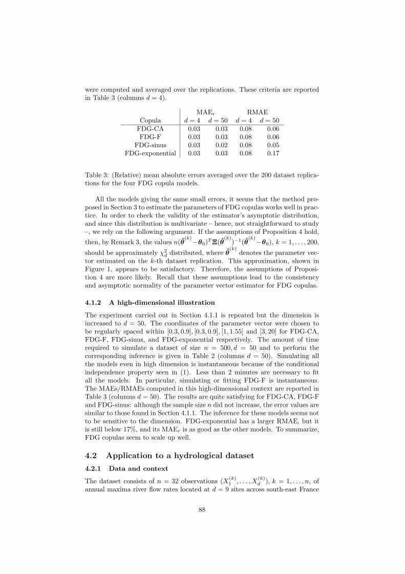
were computed and averaged over the replications. These criteria are reportedin Table 3 (columns d = 4).

MAEr RMAECopula d = 4 d = 50 d = 4 d = 50

FDG-CA 0.03 0.03 0.08 0.06FDG-F 0.03 0.03 0.08 0.06

FDG-sinus 0.03 0.02 0.08 0.05FDG-exponential 0.03 0.03 0.08 0.17

Table 3: (Relative) mean absolute errors averaged over the 200 dataset replica-tions for the four FDG copula models.

All the models giving the same small errors, it seems that the method pro-posed in Section 3 to estimate the parameters of FDG copulas works well in prac-tice. In order to check the validity of the estimator’s asymptotic distribution,and since this distribution is multivariate – hence, not straightforward to study–, we rely on the following argument. If the assumptions of Proposition 4 hold,

then, by Remark 3, the values n(θ(k)−θ0)TΞ(θ

(k))−1(θ

(k)−θ0), k = 1, . . . , 200,

should be approximately χ2d distributed, where θ

(k)denotes the parameter vec-

tor estimated on the k-th dataset replication. This approximation, shown inFigure 1, appears to be satisfactory. Therefore, the assumptions of Proposi-tion 4 are more likely. Recall that these assumptions lead to the consistencyand asymptotic normality of the parameter vector estimator for FDG copulas.

4.1.2 A high-dimensional illustration

The experiment carried out in Section 4.1.1 is repeated but the dimension isincreased to d = 50. The coordinates of the parameter vector were chosen tobe regularly spaced within [0.3, 0.9], [0.3, 0.9], [1, 1.55] and [3, 20] for FDG-CA,FDG-F, FDG-sinus, and FDG-exponential respectively. The amount of timerequired to simulate a dataset of size n = 500, d = 50 and to perform thecorresponding inference is given in Table 2 (columns d = 50). Simulating allthe models even in high dimension is instantaneous because of the conditionalindependence property seen in (1). Less than 2 minutes are necessary to fitall the models. In particular, simulating or fitting FDG-F is instantaneous.The MAEs/RMAEs computed in this high-dimensional context are reported inTable 3 (columns d = 50). The results are quite satisfying for FDG-CA, FDG-Fand FDG-sinus: although the sample size n did not increase, the error values aresimilar to those found in Section 4.1.1. The inference for these models seems notto be sensitive to the dimension. FDG-exponential has a larger RMAE, but itis still below 17%, and its MAEr is as good as the other models. To summarize,FDG copulas seem to scale up well.

4.2 Application to a hydrological dataset

4.2.1 Data and context

The dataset consists of n = 32 observations (X(k)1 , . . . , X

(k)d ), k = 1, . . . , n, of

annual maxima river flow rates located at d = 9 sites across south-east France

88

Figure 1: Histograms of n(θ(k) − θ0)TΞ(θ

(k))−1(θ

(k) − θ0), k = 1, . . . , 200,together with the density of a χ2

d distribution. From left to right, top to bottom:FDG-CA, FDG-F, FDG-sinus, and FDG-exponential.

between 1969 and 2007 (some records are missing). Let us denote by F the dis-tribution with continuous margins F1, . . . , Fd of the random vector (X1, . . . , Xd)whose realizations provide the observed dataset. The location of the sites areshown in Figure 2. The number of variable pairs is p = 36. Due to the hetero-geneous dispersion of the sites, the span of positive dependence is almost maxi-mum; for instance, Spearman’s rho dependence coefficients range from about 0to 0.9.

In hydrology, it is of interest to get information about the statistical distri-bution of a potentially dangerous event, such as {F1(X1) > q, . . . , Fd(Xd) > q},or, equivalently, {min(F1(X1), . . . , Fd(Xd)) > q}, where q is the critical levelassociated to that event. The return period T is defined as

T =1

1−M(q), where M(q) = P (min(F1(X1), . . . , Fd(Xd)) ≤ q). (21)

For instance, a return period of T = 30 years and a critical level of q = 0.7 meansthat each Xi exceeds its quantile of order 70% once every 30 years in average.A common question in the study of extreme events is the following. Given areturn period T , how dangerous is the corresponding event? In other words,

89

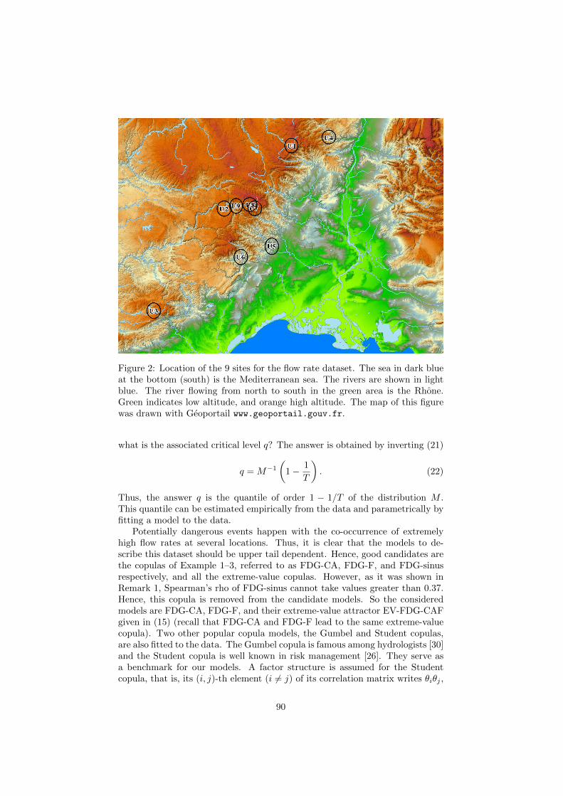
Figure 2: Location of the 9 sites for the flow rate dataset. The sea in dark blueat the bottom (south) is the Mediterranean sea. The rivers are shown in lightblue. The river flowing from north to south in the green area is the Rhone.Green indicates low altitude, and orange high altitude. The map of this figurewas drawn with Geoportail www.geoportail.gouv.fr.

what is the associated critical level q? The answer is obtained by inverting (21)

q = M−1

(1− 1

T

). (22)

Thus, the answer q is the quantile of order 1 − 1/T of the distribution M .This quantile can be estimated empirically from the data and parametrically byfitting a model to the data.

Potentially dangerous events happen with the co-occurrence of extremelyhigh flow rates at several locations. Thus, it is clear that the models to de-scribe this dataset should be upper tail dependent. Hence, good candidates arethe copulas of Example 1–3, referred to as FDG-CA, FDG-F, and FDG-sinusrespectively, and all the extreme-value copulas. However, as it was shown inRemark 1, Spearman’s rho of FDG-sinus cannot take values greater than 0.37.Hence, this copula is removed from the candidate models. So the consideredmodels are FDG-CA, FDG-F, and their extreme-value attractor EV-FDG-CAFgiven in (15) (recall that FDG-CA and FDG-F lead to the same extreme-valuecopula). Two other popular copula models, the Gumbel and Student copulas,are also fitted to the data. The Gumbel copula is famous among hydrologists [30]and the Student copula is well known in risk management [26]. They serve asa benchmark for our models. A factor structure is assumed for the Studentcopula, that is, its (i, j)-th element (i 6= j) of its correlation matrix writes θiθj ,

90

where θ1, . . . , θd belong to [−1, 1]. Recall that a Gumbel copula is an extreme-value copula. More details about the Gumbel and the Student copula can befound respectively in, e.g., [19, 27] and [8].

4.2.2 Method

A practically convenient approach dicted the estimation of the copula param-eters. For each copula model, the dependence coefficients with the simplestmathematical forms were chosen to build the loss function (18). In other words,the parameters of FDG-F and FDG-CA were estimated with Spearman’s rho asin Example 5. The parameters of EV-FDG-CAF were estimated with the ex-tremal dependence coefficient as in Example 7. The parameters of the Gumbeland Student copulas were estimated with Kendall’s tau as in Example 6. Fi-nally, the degree of freedom of the Student copula was estimated by maximizingits likelihood but with all the parameters of the correlation matrix held fixed.This approach improves the speed, tractability, and chances of success of theminimization procedure.

To be valid, the asymptotic properties of the estimator based on the ex-tremal dependence coefficients require the knowledge of the marginal distribu-tions Fi. Assuming that the data come from an extreme-value distribution,the marginal distributions theoretically pertain to the family of the GeneralizedExtreme Value (GEV) distributions. The good results of the GEV fit to thedata margins are depicted by the quantile-quantile plot in Figure 3. In addi-tion to transform the data to have standard uniform margins, these fitted GEVdistributions served to calculate the critical levels of (22) as well. This primarystep, that of fitting a parametric model to the margins, is standard in extreme-value statistics; see, for instance, [6] Chapter 8 and [29]. Details for the GEVdistribution are to be found, e.g., in [6] Chapter 3.

4.2.3 Results

The fit of the tested copulas was assessed by comparing the pairwise dependencecoefficients and the critical levels.

Pairwise dependence coefficients. The mean absolute error (MAE), de-fined as

MAEr =1

p

∑

i<j

∣∣ri,j − r(θi, θj)∣∣

was computed for Spearman’s rho (MAEρ), Kendall’s tau (MAEτ ) and theextremal dependence coefficient (MAEλ). They are reported in Table 4. MAEλwas computed only for EV-FDG-CAF and the Gumbel copula because, with thisdependence coefficient, (19) holds only for extreme-value copulas, see Example 7.The Gumbel copula has the largest errors (more than 0.17) and does not seem tofit the data well. This was expected, because this model has only one parameterto account for a d = 9 dimensional phenomenon. All the remaining errors(but MAEρ for EV-FDG-CAF) are smaller and of the same magnitude. Thus,according to these criteria, the Gumbel copula is not appropriate.

91

Figure 3: Quantile-Quantile plots with confidence intervals for the GEV fit ofthe data margins.

FDG-F FDG-CA EV-FDG-CAF Gumbel StudentMAEρ 0.12 0.12 0.17 0.22 0.12MAEτ 0.12 0.11 0.12 0.17 0.10MAEλ 0.11 0.45

Table 4: Mean absolute error for Spearman’s rho (MAEρ), Kendall’s tau(MAEτ ) and extremal (MAEλ) dependence coefficient of the models.

Critical levels. The critical levels obtained from the empirical data and themodels were calculated by making use of (22). In statistical terms, this amountsto compare the quantiles of the distribution M under the empirical data andunder the different models. The results are presented in Figure 4, where theindependence copula C(u1, . . . , ud) = u1 . . . ud was added to emphasize the needfor a joint model on such a dataset. The Gumbel model is confirmed to performpoorly. FDG-F, FDG-CA and EV-FDG-CAF seem to fit the data quite well.In particular, FDG-F and FDG-CA are as close as the Student copula to the

92

empirical curve.

Figure 4: Critical level q as a function of the return period T . “empirical” standsfor the empirical critical levels, and “independence” for the independence copulaC(u1, . . . , ud) =

∏di=1 ui.

With such a small sample size n = 32, one must be extremely careful whenlooking at empirical data, because one is likely to observe a large deviation fromthe true underlying statistical distribution. In view of this remark, one shouldselect a statistical model based not only on empirical data, but also on the modelproperties. The class of FDG copulas is very interesting in this respect. Indeed,the practitioner has with this class three models that fit well the data and withdifferent features: FDG-F is upper, lower, and symmetric tail dependent, FDG-CA is upper tail dependent but no lower tail dependent, and EV-FDG-CAF isan extreme-value copula. The user is then free to choose the model that mostsuits his expert knowledge about the underlying phenomenon at play. The testof extreme-value dependence [20] gave a p-value of 0.21, which means that onedoes not reject extreme-value copulas at the 5% level. Of course, as before, onemust be extremely careful when looking at the p-value because of the small datasample size. Regarding the possibility of testing for a given parametric family,

93

one can see [21].

5 Discussion

In this article, we have constructed a new class of copulas by combining one-factor copulas, that is, a conditional independent property, together with a classof bivariate copulas called the Durante class of bivariate copulas. This combi-nation led to many advantageous properties. The copulas within the proposedclass, referred to as FDG copulas, are tractable, flexible, and cover all typesof tail dependencies. The theoretically well grounded least-squares inferenceestimator is particularly well suited for FDG copulas because their dependencecoefficients are easy to compute, if not in closed form. This allows to performfast and reliable inference in the parametric case. We have demonstrated, fur-thermore, that FDG copulas work well in practice and are able to model bothhigh-dimensional and real datasets. Finally, we have derived the extreme-valuecopulas (EV-FDG) associated to FDG copulas, yielding a new extreme-valuecopula, which can be viewed as a generalisation of the well known Cuadras-Augecopula. This copula benefits from almost all the many advantageous propertiesof FDG copulas, and therefore opens the door for statistical analyses of extremedata in high dimension.

One may argue that a model with a singular component, as a FDG copula, isnot natural nor realistic to model hydrological data. While this may be true inthe bivariate case, this argument becomes weaker when the dimension increases.Indeed, in high-dimensional applications, the focus is less on the distributionitself than on a feature of interest of the data, such as, for instance, the criticallevels defined in (22). If alleged “unrealistic” models are able to better estimatethese features than “realistic” models – compare the fit of the Gumbel copulato the fit of FDG copulas in Section 4.2 – then one should consider using them.

This work raises several research questions. First, how to estimate the gen-erators nonparametrically? The generator of a bivariate Durante copula wasestimated nonparametrically in [10], but the matter is more complicated in ourcase because this bivariate relationship occurs between the variable of interestand the unobserved latent factor. Second, one may add more factors whenbuilding an FDG copula. Nonetheless, the model might not be as tractable asit is and therefore it may be less appealing in practice. Finally, FDG copulaspossess the conditional independence property, but the extreme-value EV-FDGcopulas were not shown to do so. If this property held, this would be of greatinterest for the simulation of datasets from this model.

Acknowledgment. The authors thank “Banque HYDRO du Ministere del’Ecologie, du Developpement durable et de l’Energie” for providing the data andBenjamin Renard for fruitful discussions about statistical issues in hydrologicalscience.

94

A Appendix

Proof of Theorem 1

Let Cj|0(·|u0) be the conditional distribution of Uj given U0 = u0. The Uj ’s areconditionally independent given U0, hence,

C(u) =

∫ 1

0

d∏

j=1

Cj|0(uj |u0)du0 (23)

=

∫ 1

0

d∏

j=1

∂C0j(u0, uj)

∂u0du0

=

∫ 1

0

d∏

j=1

∂C0(j)(u0, u(j))

∂u0du0

=

∫ u(1)

0

d∏

j=1

∂C0(j)(u0, u(j))

∂u0du0

+d∑

k=2

∫ u(k)

u(k−1)

k−1∏

j=1

∂C0(j)(u0, u(j))

∂u0

d∏

j=k

∂C0(j)(u0, u(j))

∂u0

+

∫ 1

u(d)

d∏

j=1

∂C0(j)(u0, u(j))

∂u0du0.

Since

∂C0j(u0, uj)

∂u0=

{fj(uj) if u0 < uj

ujf′j(u0) if u0 > uj ,

(23) yields

C(u) =u(1)

d∏

j=1

fj(uj) +d∑

k=2

d∏

j=k

f(j)(u(j))

∫ u(k)

u(k−1)

k−1∏

j=1

u(j)f′(j)(u0)du0

+

d∏

j=1

uj

∫ 1

u(d)

f ′j(u0)du0.

Putting u(1) in factor and noting that∫ u(2)

u(1)f ′(1)(x)dx = f(1)(u(2)) − f(1)(u(1))

finishes the proof.

Proof of Proposition 1

It suffices to set all uk equal to one but ui and uj in the formula (3).

Proof of Proposition 2

It suffices to apply the formulas (5) with fij given in Proposition 1. To computeSpearman’s rho, note that

∫ 1

0

x2fij(x)dx =

∫ 1

0

x2fi(x)fj(x)dx+

∫ 1

0

x3

∫ 1

x

f ′i(z)f′j(z)dzdx.

95

An integration by parts yields∫ 1

0x3∫ 1

xf ′i(z)f

′j(z)dzdx = (1/4)

∫ 1

0x4f ′i(x)f ′j(x)dx

and the result follows.

Proof of Theorem 2

Fix (u1, . . . , ud) ∈ [0, 1]d and let n ≥ 1 be an integer. Put

αn :=u1/n(1)

d∏

j=1

fj(u1/nj )

u1/nj

,

βn :=

∫ 1

u1/n

(d)

d∏

j=1

f ′j(u0)du0,

γn :=d∏

j=k

f(j)(u1/n(j) )

u1/n(j)

,

δn,k :=

∫ u1/n

(k)

u1/n

(k−1)

k−1∏

j=1

f ′(j)(u0)du0,

and define

An := αn + βn +

d∑

k=2

γn,kδn,k.

We are going to derive asymptotic equivalent sequences for αn, βnγn and δn.Let ∼ denote the equivalent symbol at infinity (i.e., an ∼ bn means an/bn → 1as n → ∞). By using the well known formulas ex ∼ 1 + x (when x → 0),log x ∼ x− 1 (when x→ 1) and fj(x) ∼ 1 + (x− 1)f ′j(1) (when x→ 1) we get

αn ∼(

1 +1

nlog u(1)

)(1− 1

nlog(u1 . . . ud)

)1 +

1

n

d∑

j=1

log u(j)f′(j)(1)

and

γn,k ∼

1− 1

n

d∑

j=k

log u(j)

1 +

1

n

d∑

j=k

log u(j)f′(j)(1)

.

For βn the equivalence is obtained as follows. Let F (x) be a primitive of∏dj=1 f

′j(x). It follows that βn = F (1)− F (u

1/n(d) ). A Taylor expansion yields

F (u1/n(d) ) = F (1) + (u

1/n(d) − 1)F ′(1) +

(u1/n(d) − 1)2

2F ′′(xn)

where xn is between u1/n(d) and 1. Since F ′′ is assumed to be continuous on [0, 1],

it is uniformly bounded on this set and therefore (u1/n(d) − 1)2F ′′(xn)/2 = o(1/n)

where o(1/n) is a quantity such that no(1/n) → 0 as n → ∞. Hence, since

u1/n(d) = exp(log(u(d))/n) ∼ 1 + log(u(d))/n, we have as n→∞

F (1)− F (u1/n(d) ) ∼ − 1

nlog(u(d))F

′(1).

96

The same arguments apply to get

βn ∼ −1

nlog u(d)

d∏

j=1

f ′j(1)

δn,k ∼1

nlog

(u(k)

u(k−1)

) k−1∏

j=1

f ′(j)(1).

The quantity An is a polynomial with respect to n−1 of order at most three.In (24), the coefficients of order 0, 2, and 3 vanish at infinity. Only remain theterms of order 1, hence,

limn↑∞

n(An − 1) = log u(1) − log(u1 . . . ud) +

d∑

j=1

log u(j)f′(j)(1) (24)

− log u(d)

d∏

j=1

f ′(j)(1) +d∑

k=2

k−1∏

j=1

f ′(j)(1) log

(u(k)

u(k−1)

).

From Abel’s identity, that is,∑d−1i=1 ai(bi+1−bi) =

∑d−1i=1 bi(ai−1−ai)+ad−1bd−

a1b1 for two sequences (ai) and (bi) of real numbers, we can write

limn↑∞

n(An − 1) =

d∑

k=1

k−1∏

j=1

f ′(j)(1)

(1− f ′(k)(1)) + f ′(k)(1)− 1

︸ ︷︷ ︸=:χk

log u(k),

with the convention that∏0j=1 f

′(j)(1) = 1. From (3) it follows that

Cn(u1/n1 , . . . , u

1/nd ) =u1 . . . ud exp [n logAn]

=u1 . . . ud exp [n(An − 1)(1 + o(1))]

→d∏

i=k

uχk

(k)

as n→∞.

Proof of Lemma 1

(i) Since the p-uple (r1,2, . . . , rd−1,d) belongs to the image space r(Θd), thesystem

r(θ1, θ2) =r1,2

...

r(θd−1, θd) =rd−1,d

has at least one solution. In particular, there exists (θ1, θ2, θ3) in Θ3 such that

r(θ1, θ2) =r1,2

r(θ1, θ3) =r1,3

r(θ2, θ3) =r2,3. (25)

97

The system (25) rewrites

rθ2(θ1) =r1,2

rθ3(θ1) =r1,3

rθ3(θ2) =r2,3,

or equivalently,

θ1 =s1,2(θ2)

θ1 =s1,3(θ3)

θ2 =s2,3(θ3).

This yields

s1,3(θ3) = s1,2 ◦ s2,3(θ3). (26)

Note that s1,3 is involutive at θ3, that is, s1,3 ◦s1,3(θ3) = θ3. Indeed, r(θ1, θ3) =rθ3(θ1) = r1,3 is equivalent to θ1 = r−1

θ3(r1,3) = s1,3(θ3). This implies r(s1,3(θ3), θ3) =

r1,3, and, composing by r−1s1,3(θ3) in both sides, we get r−1

s1,3(θ3)(r1,3) = s1,3(s1,3(θ3)) =

θ3. Therefore, one can compose both sides of (26) by s1,3 to get

θ3 = s1,3 ◦ s1,2 ◦ s2,3(θ3).

Hence (20) has at least one solution.(ii) If (20) admits exactly one solution θ3, then θ2 and θ1 are also unique.

Furthermore, for all j ≥ 3,

θj+1 = sj,j+1(θj)

which concludes the proof that assumption (A1) holds. It is now shown thatassumption (A2) holds as well. Define ∂1r, respectively, ∂2r, the derivative of rwith respect to the first, respectively, second, variable of r. Hence for all θi andθj in Θ, the quantities ∂1r(θi, θj) and rθj (θi) only differ in the notation. Thefirst step in the proof is to consider the case d = 3. The Jacobian matrix of rat θ0 is given by

J =

∂1r(θ01, θ02) ∂2r(θ01, θ02) 0∂1r(θ01, θ03) 0 ∂2r(θ01, θ03)

0 ∂1r(θ02, θ03) ∂2r(θ02, θ03)

.

To show that J has full rank, we show that its determinant

∂1r(θ01, θ02)∂2r(θ01, θ03)∂1r(θ02, θ03) + ∂2r(θ02, θ03)∂1r(θ01, θ03)∂2r(θ01, θ02)

is nonzero. Indeed, note that for all θ in Θ, the map rθ : Θ→ rθ(Θ) is a twicecontinuously differentiable homeomorphism. Furthermore, by assumption, thetrue parameter vector θ0 lies in the interior of Θ that is open. Finally, bysymmetry, for all i < j,

∂r1(θ0i, θ0j) > 0 (respectively ∂r1(θ0i, θ0j) < 0)

is equivalent to

∂r2(θ0j , θ0i) > 0 (respectively ∂r2(θ0j , θ0i) < 0).

98

For the general case, we proceed by mathematical induction. When thedimension is d, write J(θ) = J(d)(θ) to emphasize the dependence on the di-mension. Notice that it was already shown above that J(3)(θ) has full rank.Now suppose that the kernel of J(d−1)(θ) is null when the dimension is d − 1.Let A = J(d)(θ). Each row of A writes

(0, . . . , 0, ∂1r(θi, θj), 0 . . . , 0, ∂2r(θi, θj), 0, . . . , 0)

where ∂1r(θi, θj) is at the i-th position and ∂2r(θi, θj) at the j-th position.There are d−1 rows of A which depend on θd and p−d+1 which do not (recallp = d(d− 1)/2 is the number of pairs). Since the kernel of a matrix is invariantby permutation, we can without loss of generality put all the rows which do notdepend on θd on the top. More precisely, decompose A as

A =

(A11 A12

A21 A22

)

such that A11 is a (p− d+ 1)× (d− 1) matrix containing all the rows which donot depend on θd and A12 and A22 are (p− d+ 1)× 1 and (d− 1)× 1 matricesrespectively. Note that A12 is the null vector of size p− d+ 1× 1. Let x ∈ Rd,x = (xT1 , x2)T where x1 ∈ Rd−1, x2 ∈ R. It follows that Ax = 0 is equivalentto

{A11x1 + A12x2 = 0A21x1 + A22x2 = 0.

But A12 = 0 and since A11 = J(d−1)(θ) whose kernel is null, x1 = 0. ThenA22x2 = 0 and the assumptions imply x2 = 0, which concludes the proof.

Proof of Corollary 1

To prove Corollary 1, it suffices to apply Lemma 1. Since r(θi, θj) denotes theextremal dependence coefficient of the E copula bivariate marginal C#,ij definedin (16), we have

r(θi, θj) = λ(θi)λ(θj), where

λ(θ) := 1− ∂f(t, θ)

∂t

∣∣∣t=1

. (27)

In the Cuadras-Auge and the Frechet cases, (27) is given by λ(θ) = θ, and in thesinus case, λ(θ) = 1− θ/ tan(θ). In all these situations, it is easy to see that themap rθj (·) is a twice continuously differentiable homeomorphism. Therefore,Lemma 1 (i) applies.

To apply the second part of Lemma 1, note that equation (20) translatesinto

λ(θ)2 =r1,3r2,3

r1,2.

Since it has a unique solution, Lemma 1 (ii) applies, and the result is proved.

99

References

[1] K. Aas, C. Czado, A. Frigessi, and H. Bakken. Pair-copula constructions ofmultiple dependence. Insurance: Mathematics and Economics, 44(2):182–198, 2009.

[2] E. F. Acar, C. Genest, and J. NesLehova. Beyond simplified pair-copulaconstructions. Journal of Multivariate Analysis, 110:74–90, 2012.

[3] C. Amblard and S. Girard. A new extension of bivariate FGM copulas.Metrika, 70(1):1–17, 2009.

[4] T. Bedford and R.M. Cooke. Probability density decomposition for condi-tionally dependent random variables modeled by vines. Annals of Mathe-matics and Artificial intelligence, 32(1-4):245–268, 2001.

[5] T. Bedford and R.M. Cooke. Vines–a new graphical model for dependentrandom variables. The Annals of Statistics, 30(4):1031–1068, 2002.

[6] S. Coles. An introduction to statistical modeling of extreme values. Springer,2001.

[7] C.M. Cuadras and J. Auge. A continuous general multivariate distributionand its properties. Communications in Statistics - Theory and Methods,10(4):339–353, 1981.

[8] S. Demarta and A. J. McNeil. The t copula and related copulas. Interna-tional statistical review, 73(1):111–129, 2005.

[9] F. Durante. A new class of symmetric bivariate copulas. NonparametricStatistics, 18(7-8):499–510, 2006.

[10] F. Durante and O. Okhrin. Estimation procedures for exchangeable mar-shall copulas with hydrological application. Stochastic Environmental Re-search and Risk Assessment, published online, 2014.

[11] F. Durante, J.J. Quesada-Molina, and M. Ubeda Flores. On a familyof multivariate copulas for aggregation processes. Information Sciences,177(24):5715–5724, 2007.

[12] F. Durante and G. Salvadori. On the construction of multivariate extremevalue models via copulas. Environmetrics, 21(2):143–161, 2010.

[13] M. Ferreira. Nonparametric estimation of the tail-dependence coefficient.REVSTAT–Statistical Journal, 11(1):1–16, 2013.

[14] G. Frahm, M. Junker, and A. Szimayer. Elliptical copulas: applicabilityand limitations. Statistics & Probability Letters, 63(3):275–286, 2003.

[15] M. Frechet. Remarques au sujet de la note precedente. CR Acad. Sci. ParisSer. I Math, 246:2719–2720, 1958.

[16] C. Genest and A. C. Favre. Everything you always wanted to know aboutcopula modeling but were afraid to ask. Journal of Hydrologic Engineering,12(4):347–368, 2007.

100

[17] G. Gudendorf and J. Segers. Extreme-value copulas. In P. Jaworski, F. Du-rante, W.K. Hardle, and T. Rychlik, editors, Copula Theory and Its Appli-cations, page 127–145. Springer, 2010.

[18] W. Hoeffding. A class of statistics with asymptotically normal distribution.The Annals of Mathematical Statistics, 19(3):293–325, 1948.

[19] H. Joe. Multivariate models and dependence concepts. Chapman &Hall/CRC, Boca Raton, FL, 2001.

[20] I. Kojadinovic, J. Segers, and J. Yan. Large-sample tests of extreme-value dependence for multivariate copulas. Canadian Journal of Statistics,39(4):703–720, 2011.

[21] I. Kojadinovic and J. Yan. A goodness-of-fit test for multivariate multipa-rameter copulas based on multiplier central limit theorems. Statistics andComputing, 21(1):17–30, 2011.

[22] P. Krupskii and H. Joe. Factor copula models for multivariate data. Journalof Multivariate Analysis, 120:85–101, 2013.

[23] D. Kurowicka and R.M. Cooke. Distribution-free continuous Bayesian beliefnets. In Proceedings of Mathematical methods in Reliability Conference,Santa Fe, New Mexico, USA, 2004.

[24] J.F. Mai and M. Scherer. Levy-frailty copulas. Journal of MultivariateAnalysis, 100(7):1567–1585, 2009.

[25] G. Mazo, S. Girard, and F. Forbes. Weighted least-squares inference basedon dependence coefficients for multivariate copulas. http://hal.archives-ouvertes.fr/hal-00979151, 2014.

[26] A.J. McNeil, R. Frey, and P. Embrechts. Quantitative risk management:concepts, techniques, and tools. Princeton university press, 2010.

[27] R.B. Nelsen. An introduction to copulas. Springer, New York, 2006.

[28] R Core Team. R: A Language and Environment for Statistical Computing.R Foundation for Statistical Computing, Vienna, Austria, 2013.

[29] B. Renard and M. Lang. Use of a Gaussian copula for multivariate ex-treme value analysis: some case studies in hydrology. Advances in WaterResources, 30(4):897–912, 2007.

[30] L. Zhang and V. P. Singh. Gumbel–Hougaard copula for trivariate rainfallfrequency analysis. Journal of Hydrologic Engineering, 12(4):409–419, 2007.

101

Conclusion

Dans cette thèse, nous avons proposé deux nouvelles classes de copules. Lapremière est construite à partir d’une classe prenant la forme d’un produit géné-ralisé de copules. Etant reconnu que cette classe doit être simplifiée pour pouvoirêtre utile en pratique, nous avons montré que, si les fonctions gei de Liebscherne dépendent en fait pas de l’indice e, et si l’on souhaite tirer profit de la largegamme de familles de copules bivariées disponibles dans la littérature, alors laseule classe possible que l’on peut construire est la classe des copules PBC duchapitre 4. De plus, nous avons montré le lien avec un algorithme message-passing, ce qui permet de faire l’estimation des copules PBC par maximum devraisemblance. Toutefois, nous avons montré également que les copules PBC nesont pas capables de modéliser des variables très dépendantes, et, par consé-quent, sont d’une utilité limitée pour les applications.

La deuxième classe de copules que nous avons proposées (les copules FDG)est, à notre avis, beaucoup plus intéressante pour les applications. En effet,cette classe est très maniable, parcimonieuse – puisque le nombre de paramètresn’augmente que proportionnellement par rapport à la dimension –, et les ex-pressions des coefficients de dépendance sont explicites, ce qui permet d’étudieret de quantifier la dépendance avec aisance. Nous avons montré que la classeFDG permet d’obtenir des dépendances dans les queues inférieures mais passupérieures, ou l’inverse, ou les deux. Les variables d’intérêts sont conditionnel-lement indépendantes par rapport à un facteur latent, ce qui permet de simulertrès facilement selon ces copules. Ce facteur latent peut être ignoré, ou peut êtrevu comme un attrait supplémentaire du modèle en cela qu’il facilite son inter-prétation. Enfin, les copules FDG présentent une composante singulière. Ellespeuvent donc être utilisées dans le cadre de modèles à chocs, comme vu dansla partie 1.3.2. Mais nous avons montré que les copules FDG peuvent aussi êtreutilisées avec succès dans des applications de natures différentes, c’est à dire,même quand il n’y a pas de chocs. En particulier, nous avons estimé le niveaucritique associé aux évènements de débits extrêmes de la région des Cévennes(sud de la France). Nos résultats sont robustes à l’intérieur de la classe FDG,ajustent bien les données, et sont en cohérence avec les résultats obtenus avecune copule de Student. Enfin, nous avons montré que l’on pouvait calculer lescopules extrêmes associées aux copules FDG (les copules EV-FDG), enrichis-sant ainsi la gamme des copules extrêmes, d’autant que les copules extrêmesissues des copules FDG réalisent elles aussi un bon compromis entre flexibilitéet maniabilité. Elles ont d’ailleurs été testées et utilisées en pratique au mêmetitre que les autres copules.

Dans le cadre de cette thèse, nous avons également apporté notre contri-bution à l’estimation de copules. Nous avons souligné que les méthodes ac-

102

tuelles d’estimation n’avaient pas de fondements théoriques si les copules consi-dérées n’ont pas de dérivées partielles, ce qui est le cas des copules FDG. Nousavons montré que, sous des conditions d’identifiabilité naturelles, l’estimateurdes moindres carrés pondérés basé sur les coefficients de dépendance existe etest unique avec une probabilité s’approchant de 1 au fur et à mesure que la taillede l’échantillon augmente, et qu’il était asymptotiquement consistant et normal,et ce, même si les copules considérées n’admettent pas de dérivées partielles.

Les perspectives à nos différents travaux ont été discutées dans les chapitresles concernant. Pour les copules PBC, il avait été suggéré que ces dernièresétaient peut-être d’un intérêt plus théorique que pratique. Concernant les co-pules FDG, avait été posé la question de l’estimation non paramétrique desgénérateurs. Nous avions aussi fait remarquer que plusieurs facteurs cachés pour-raient être envisagés lors la construction de ces copules, mais que cela risqueraitde les rendre moins maniables. La propriété d’indépendance conditionnelle, éta-blie (par construction) pour les copules FDG, n’a pas été démontrée pour lescopules EV-FDG. Or si cette propriété était vraie, elle serait utile, entre autre,pour simuler des données selon ces copules. Enfin, concernant l’estimateur desmoindres carrés basé sur les coefficients de dépendance, l’application hydrolo-gique a révélé que ce dernier pouvait être instable numériquement lorsque lenombre de paramètres à estimer est égal aux nombre de paires de variables.Dans ce cas, on pourrait envisager une combinaison de coefficients de différentstypes (rho de Spearman, tau de Kendall...) afin de rendre le système d’équationsà résoudre plus robuste numériquement.

Nos travaux s’inscrivent dans un contexte plus global, dont nous faisons unesynthèse ci-dessous. La recherche de modèles multivariés avec autant de qualitésque possible était un sujet important il y a une dizaine d’années. Nous avons lesentiment, que, de nos jours, il en existe une gamme assez diversifiée. Ces toutesdernières années, en particulier, ont vu apparaitre une classe de modèles trèsflexibles, les Vines. Bien sûr, il reste encore beaucoup de recherche à effectuer,notamment pour rendre ces modèles plus parcimonieux, et mieux comprendreleur sensibilité par rapport au choix de la décomposition de la densité, ou desfamilles paramétriques bivariées à incorporer. En outre, le risque est grand,avec ces modèles, de sur-ajuster (overfit en anglais) les données. En ce sens,les modèles à facteur, et en particulier à un facteur (comme celui que nousavons proposé), sont très intéressants. Ils peuvent d’ailleurs être vus commedes modèles Vines « tronqués ». Nous aimerions terminer cette thèse par lequestionnement « méta-statistique » suivant : que voulons-nous faire avec nosmodèles ? Le but est-il vraiment d’ajuster les données le mieux possible, commeil en ressort l’impression à la lecture de certaines publications ? A notre avis, engrande dimension, la distribution que nous tentons de modéliser nous importemoins qu’une caractéristique de cette dernière. Autrement dit, c’est moins laloi de (X1, . . . , Xd) que celle de ϕ(X1, . . . , Xd), avec ϕ : Rd 7→ R, qui nousintéresse. Par exemple, dans le cas des applications en hydrologie que nousavons traitées à plusieurs reprises dans cette thèse, nous avons ϕ(X1, . . . , Xd) =min(X1, . . . , Xd). Il y a trois possibilités d’estimer la loi de ϕ(X1, . . . , Xd) :

1. en utilisant un historique des données de ϕ(X1, . . . , Xd) lui même,2. en modélisant la loi de ϕ(X1, . . . , Xd) elle même, ou,3. en modélisant la loi de (X1, . . . , Xd).

C’est seulement dans la dernière situation que nous avons besoin d’un modèle

103

multivarié, et si c’était cas, ce modèle devrait être choisi aussi en fonction deses capacités relativement à la fonctionnelle ϕ, et pas seulement relativement àses capacités à « ajuster les données ». Même un modèle a priori peu flexiblepeux donner des résultats satisfaisants. La reproductibilité des résultats, enparticulier, doit être vérifiée avec attention.

104

Bibliographie

[1] K. Aas, C. Czado, A. Frigessi, and H. Bakken. Pair-copula constructions ofmultiple dependence. Insurance : Mathematics and Economics, 44(2) :182–198, 2009.

[2] E. F. Acar, C. Genest, and J. NešLehová. Beyond simplified pair-copulaconstructions. Journal of Multivariate Analysis, 110 :74–90, 2012.

[3] C. Amblard and S. Girard. A new extension of bivariate FGM copulas.Metrika, 70(1) :1–17, 2009.

[4] T. Bedford and R. M. Cooke. Probability density decomposition for condi-tionally dependent random variables modeled by vines. Annals of Mathe-matics and Artificial intelligence, 32(1-4) :245–268, 2001.

[5] T. Bedford and R. M. Cooke. Vines : A new graphical model for dependentrandom variables. Annals of Statistics, 30(4) :1031–1068, 2002.

[6] D. Berg. Copula goodness-of-fit testing : an overview and power compari-son. The European Journal of Finance, 15(7-8) :675–701, 2009.

[7] L. Breiman. Statistical modeling : The two cultures (with comments anda rejoinder by the author). Statistical Science, 16(3) :199–231, 2001.

[8] A. Bücher, H. Dette, and S. Volgushev. New estimators of the Pickandsdependence function and a test for extreme-value dependence. The Annalsof Statistics, 39(4) :1963–2006, 2011.

[9] P. Capéraà, A. L. Fougères, and C. Genest. A nonparametric estimationprocedure for bivariate extreme value copulas. Biometrika, 84(3) :567–577,1997.

[10] D. G. Clayton. A model for association in bivariate life tables and itsapplication in epidemiological studies of familial tendency in chronic diseaseincidence. Biometrika, 65(1) :141–151, 1978.

[11] S. Coles. An introduction to statistical modeling of extreme values. Springer,2001.

[12] C. M. Cuadras and J. Augé. A continuous general multivariate distributionand its properties. Communications in Statistics - Theory and Methods,10(4) :339–353, 1981.

[13] L. de Haan and A. Ferreira. Extreme value theory : an introduction. Sprin-ger, 2007.

[14] P. Deheuvels. A nonparametric test for independence. Publications del’Institut de Statistique de l’Université de Paris, 26 :29–50, 1981.

105

[15] P. Deheuvels. On the limiting behavior of the Pickands estimator forbivariate extreme-value distributions. Statistics & Probability Letters,12(5) :429–439, 1991.

[16] S. Demarta and A. J. McNeil. The t copula and related copulas. Interna-tional Statistical Review, 73(1) :111–129, 2005.

[17] F. Durante. A new class of symmetric bivariate copulas. NonparametricStatistics, 18(7-8) :499–510, 2006.

[18] F. Durante and O. Okhrin. Estimation procedures for exchangeable Mar-shall copulas with hydrological application. Stochastic Environmental Re-search and Risk Assessment, published online, 2014.

[19] F. Durante, J. J. Quesada-Molina, and M. Úbeda Flores. On a familyof multivariate copulas for aggregation processes. Information Sciences,177(24) :5715–5724, December 2007.

[20] F. Durante and G. Salvadori. On the construction of multivariate extremevalue models via copulas. Environmetrics, 21(2) :143–161, 2010.

[21] D. Fantazzini. The effects of misspecified marginals and copulas on com-puting the value at risk : A monte carlo study. Computational Statistics &Data Analysis, 53(6) :2168–2188, 2009.

[22] J. D. Fermanian, D. Radulovic, and M. Wegkamp. Weak convergence ofempirical copula processes. Bernoulli, 10(5) :847–860, 2004.

[23] G. Frahm, M. Junker, and A. Szimayer. Elliptical copulas : applicabilityand limitations. Statistics & Probability Letters, 63(3) :275–286, 2003.

[24] M. Fréchet. Remarques au sujet de la note précédente. Compte Rendu del’Académie des Sciences de Paris, Série I, Mathématique, 246 :2719–2720,1958.

[25] C. Genest and A. Favre. Everything you always wanted to know aboutcopula modeling but were afraid to ask. Journal of Hydrologic Engineering,12(4) :347–368, 2007.

[26] C. Genest, K. Ghoudi, and L. P. Rivest. A semiparametric estimation pro-cedure of dependence parameters in multivariate families of distributions.Biometrika, 82(3) :543–552, 1995.

[27] C. Genest, J. Nešlehová, and N. Ben Ghorbal. Estimators based on Ken-dall’s tau in multivariate copula models. Australian & New Zealand Journalof Statistics, 53(2) :157–177, 2011.

[28] C. Genest and B. Rémillard. Validity of the parametric bootstrap forgoodness-of-fit testing in semiparametric models. Annales de l’InstitutHenri Poincaré : Probabilités et Statistiques, 44(6) :1096–1127, 2008.

[29] C. Genest, B. Rémillard, and D. Beaudoin. Goodness-of-fit tests for copu-las : A review and a power study. Insurance : Mathematics and economics,44(2) :199–213, 2009.

[30] C. Genest and L. P. Rivest. Statistical inference procedures for bivariateArchimedean copulas. Journal of the American statistical Association,88(423) :1034–1043, 1993.

[31] C. Genest and J. Segers. Rank-based inference for bivariate extreme-valuecopulas. The Annals of Statistics, 37(5B) :2990–3022, 2009.

106

[32] C. Genest and B. J. M. Werker. Conditions for the asymptotic semipa-rametric efficiency of an omnibus estimator of dependence parameters incopula models. In C. M. Cuadras and J. A. R. Lallena, editors, Proceedingsof the Conference on Distributions With Given Marginals and StatisticalModelling, pages 103–112, Kluwer Academic Publishers, Dordrecht, 2002.

[33] G. Gudendorf and J. Segers. Extreme-value copulas. In P. Jaworski, F. Du-rante, W. K. Härdle, and T. Rychlik, editors, Copula Theory and Its Ap-plications, page 127–145. Springer, 2010.

[34] G. Gudendorf and J. Segers. Nonparametric estimation of an extreme-value copula in arbitrary dimensions. Journal of Multivariate Analysis,102(1) :37–47, 2011.

[35] G. Gudendorf and J. Segers. Nonparametric estimation of multivariateextreme-value copulas. Journal of Statistical Planning and Inference,142(12) :3073–3085, 2012.

[36] E. J. Gumbel. Distributions des valeurs extrêmes en plusieurs dimensions.Publications de l’Institut de Statistique de l’Université de Paris, 9 :171–173,1960.

[37] I. H. Haff and J. Segers. Nonparametric estimation of pair-copula construc-tions with the empirical pair-copula. arXiv preprint :1201.5133, 2012.

[38] P. Hall and N. Tajvidi. Distribution and dependence-function estimationfor bivariate extreme-value distributions. Bernoulli, 6(5) :835–844, 2000.

[39] W. Hoeffding. A class of statistics with asymptotically normal distribution.The Annals of Mathematical Statistics, 19(3) :293–325, 1948.

[40] M. Hofert. Construction and sampling of nested Archimedean copulas. InP. Jaworski, F. Durante, W. K. Härdle, and T. Rychlik, editors, CopulaTheory and Its Applications, pages 147–160. Springer, 2010.

[41] M. Hofert, I. Kojadinovic, M. Maechler, and J. Yan. copula : MultivariateDependence with Copulas, 2014. R package version 0.999-8.

[42] M. Hofert, M. Mächler, and A. J. McNeil. Archimedean copulas in highdimensions : Estimators and numerical challenges motivated by financialapplications. Journal de la Société Française de Statistique, 154(1) :25–63,2012.

[43] M. Hofert and M. Scherer. CDO pricing with nested Archimedean copulas.Quantitative Finance, 11(5) :775–787, 2011.

[44] P. D. Hoff, X. Niu, and J. A. Wellner. Information bounds for Gaussiancopulas. Bernoulli, 20(2) :604–622, 2014.

[45] J. C. Huang, N. Jojic, and C. Meek. Exact inference and learning forcumulative distribution functions on loopy graphs. Neural InformationProcessing Systems, 2010.

[46] Li J., Das K., Fu G., Li R., and Wu R. The Bayesian lasso for genome-wideassociation studies. Bioinformatics, 27(4) :516–523, 2010.

[47] H. Joe. Multivariate models and dependence concepts. Chapman &Hall/CRC, 2001.

[48] H. Joe. Dependence Modeling with Copulas. CRC Press, 2014.[49] C. H. Kimberling. A probabilistic interpretation of complete monotonicity.

Aequationes Mathematicae, 10(2) :152–164, 1974.

107

[50] C. A. J. Klaassen and J. A. Wellner. Efficient estimation in the bivariatenormal copula model : normal margins are least favourable. Bernoulli,3 :55–77, 1997.

[51] C. Klüppelberg and G. Kuhn. Copula structure analysis. Journal of theRoyal Statistical Society : Series B (Statistical Methodology), 71(3) :737–753, 2009.

[52] I. Kojadinovic, J. Segers, and J. Yan. Large-sample tests of extreme-value dependence for multivariate copulas. Canadian Journal of Statistics,39(4) :703–720, 2011.

[53] I. Kojadinovic and J. Yan. A goodness-of-fit test for multivariate multipa-rameter copulas based on multiplier central limit theorems. Statistics andComputing, 21(1) :17–30, 2011.

[54] I. Kojadinovic and J. Yan. copula : Multivariate dependence with copulas.R package, 2014.

[55] I. Kojadinovic, J. Yan, and M. Holmes. Fast large-sample goodness-of-fittests for copulas. Statistica Sinica, 21(2) :841–871, 2011.

[56] D. Kundu and A. K. Dey. Estimating the parameters of the Marshall–Olkinbivariate Weibull distribution by EM algorithm. Computational Statistics& Data Analysis, 53(4) :956–965, 2009.

[57] D. Kurowicka. Introduction : Dependence Modeling. In D. Kurowickaand H. Joe, editors, Dependence Modeling, Vine Copula Handbook. WorldScientific, 2011.

[58] D. Kurowicka and R.M. Cooke. Distribution-free continuous Bayesian beliefnets. In Proceedings of Mathematical methods in Reliability Conference,Santa Fe, New Mexico, USA, 2004.

[59] D. Kurowicka and H. Joe, editors. Vine Copula Handbook. World Scientific,2011.

[60] O. Ledoit and Wolf M. Improved estimation of the covariance matrix ofstock returns with an application to portfolio selection. Journal of Empi-rical Finance, 10(5) :603–621, 2003.

[61] D. X. Li. On default correlation : A copula function approach. The Journalof Fixed Income, 9(4) :43–54, 2000.

[62] E. Liebscher. Construction of asymmetric multivariate copulas. Journal ofMultivariate Analysis, 99(10) :2234–2250, 2008.

[63] F. Lindskog, A. McNeil, and U. Schmock. Kendall’s tau for elliptical dis-tributions. Springer, 2003.

[64] A. W. Marshall and I. Olkin. A multivariate exponential distribution.Journal of the American Statistical Association, 62(317) :30–44, 1967.

[65] A. J. Mc Neil. Quantitative risk management : concepts, techniques andtools. Princeton series in finance. Princeton University Press, Princeton,N.J, 2005.

[66] A. J. McNeil, R. Frey, and P. Embrechts. Quantitative risk management :concepts, techniques, and tools. Princeton university press, 2010.

[67] A. J. McNeil and J. Nešlehová. Multivariate Archimedean copulas, d-monotone functions and l1-norm symmetric distributions. The Annals ofStatistics, 37(5B) :3059–3097, 2009.

108

[68] A.J. McNeil. Sampling nested Archimedean copulas. Journal of StatisticalComputation and Simulation, 78(6) :567–581, 2008.

[69] R. B. Nelsen. An introduction to copulas. Springer, 2006.[70] D. H. Oh and A. J. Patton. Modelling dependence in high dimensions with

factor copulas. Manuscript, Duke University, 2012.[71] D. H. Oh and A. J. Patton. Simulated method of moments estimation

for copula-based multivariate models. Journal of the American StatisticalAssociation, 108(502) :689–700, 2013.

[72] O. Okhrin, Y. Okhrin, and W. Schmid. On the structure and estimation ofhierarchical Archimedean copulas. Journal of Econometrics, 173(2) :189–204, 2013.

[73] J. Pickands. Multivariate extreme value distributions. In Proceedings 43rdSession International Statistical Institute, volume 2, pages 859–878, 1981.

[74] J. F. Quessy, M. Said, and A. C. Favre. Multivariate Kendall’s tau forchange point detection in copulas. The Canadian journal of statistics,41 :65–82, 2013.

[75] R Core Team. R : A Language and Environment for Statistical Computing.R Foundation for Statistical Computing, Vienna, Austria, 2013.

[76] S. I. Resnick. Extreme values, regular variation, and point processes. Sprin-ger, 2007.

[77] G. Salvadori and C. De Michele. Estimating strategies for multiparametermultivariate extreme value copulas. Hydrology and Earth System Sciences,15(1) :141–150, 2011.

[78] C. Savu and M. Trede. Hierarchies of Archimedean copulas. QuantitativeFinance, 10(3) :295–304, 2010.

[79] F. Schmid and R. Schmidt. Multivariate extensions of Spearman’s rho andrelated statistics. Statistics & Probability Letters, 77(4) :407–416, 2007.

[80] J. Segers. Asymptotics of empirical copula processes under non-restrictivesmoothness assumptions. Bernoulli, 18(3) :764–782, 2012.

[81] J. Segers, R. V. D. Akker, and B. J. M. Werker. Semiparametric Gaus-sian copula models : Geometry and rank-based efficient estimation. arXivpreprint :1306.6658, 2013.

[82] R. J. Serfling. Approximation theorems of mathematical statistics. Wiley,1980.

[83] F. Serinaldi and S. Grimaldi. Fully nested 3-copula : procedure and appli-cation on hydrological data. Journal of Hydrologic Engineering, 12(4) :420–430, 2007.

[84] J. Shao. Mathematical Statistics. Springer, 1999.[85] M. Sibuya. Bivariate extreme statistics. Annals of the Institute of Statistical

Mathematics, 11 :195–210, 1960.[86] A. Sklar. Fonction de répartition dont les marges sont données. Publications

de l’Institut de Statistique de l’Université de Paris, 8 :229–231, 1959.[87] T. Van Pham and G. Mazo. PBC : product of bivariate copulas.

http ://cran.r-project.org, 2014. R package version 1.2.[88] Science Watch. http://archive.sciencewatch.com/dr/tt/2010/

10dectt-MATH/.

109