ConstructingDualitiesfromQuantumState Manifolds · PDF filemodels is developed with the aim of...
145
arXiv:1509.01231v1 [hep-th] 2 Sep 2015 Constructing Dualities from Quantum State Manifolds by Hendrik Jacobus Rust van Zyl Dissertation presented for the degree of Doctor of Philosophy in Science in the Faculty of Science at Stellenbosch University Prof. F.G. Scholtz Dr. J.N. Kriel December 2015
Transcript of ConstructingDualitiesfromQuantumState Manifolds · PDF filemodels is developed with the aim of...
arX
iv:1
509.
0123
1v1
[he
p-th
] 2
Sep
201
5
Constructing Dualities from Quantum StateManifolds
by
Hendrik Jacobus Rust van Zyl
Dissertation presented for the degree of Doctor of
Philosophy in Science in the Faculty of Science at
Stellenbosch University
Prof. F.G. Scholtz
Dr. J.N. Kriel
December 2015
Declaration
By submitting this dissertation electronically, I declare that the entirety of the workcontained therein is my own, original work, that I am the sole author thereof (saveto the extent explicitly otherwise stated), that reproduction and publication thereofby Stellenbosch University will not infringe any third party rights and that I havenot previously in its entirety or in part submitted it for obtaining any qualification.
Date: . . . . . . . . . . . . . . . . . . . . . . . . . . . . . . . . . .
Copyright c© 2015 Stellenbosch UniversityAll rights reserved.
1
Abstract
Constructing Dualities from Quantum State Manifolds
HJR van Zyl
Dissertation: PhD
December 2015
A constructive procedure to build gravitational duals from quantum mechanicalmodels is developed with the aim of studying aspects of the gauge/gravity duality.The construction is simplified as far as possible - the most notable simplificationbeing that quantum mechanical models are considered as opposed to quantum fieldtheories. The simplifications allow a systematic development of the constructionwhich provides direct access to the quantum mechanics / gravity dictionary.The procedure is divided into two parts. First a geometry is constructed from a fam-ily of quantum states such that the symmetries of the quantum mechanical statesare encoded as isometries of the metric. Secondly, this metric is interpreted as themetric that yields a stationary value for the dual gravitational action. If the quan-tum states are non-normalisable then these states need to be regularised in order todefine a sensible metric. These regularisation parameters are treated as coordinateson the manifold of quantum states. This gives rise to the idea of a manifold “bulk”where the states are normalisable and of a “boundary” where they are not. Asymp-totically anti-de Sitter geometries arise naturally from non-normalisable states butthe geometries can also be much more general.Time-evolved states are the initial interest. A sensible regularisation scheme forthese states is a simple complexification of time so that the bulk coordinate hasthe interpretation of an energy scale. These two-dimensional manifolds of statesare dual to models of dilaton gravity where the dilaton has the interpretation ofthe expectation value of a quantum mechanical operator. As an example, statestime-evolving under an su(1, 1) Hamiltonian is dual to dilaton gravity on AdS2, inagreement with existing work on the AdS2/CFT1 correspondence. These existingresults are revisited with the aid of the systematic quantum mechanics / dilatongravity dictionary and extended. As another example, states time-evolving underan su(2) Hamiltonian are shown to be dual to dilaton gravity on dS2.The higher dimensional analysis is restricted, for computational reasons, to the ex-ample of states that possess full Schrodinger symmetry with and without dynamicalmass. The time and spatial coordinates are complexified in order to both regularisethe states and maintain the state symmetries as bulk isometries. Dictionaries aredeveloped for both examples. It is shown that submanifolds of these state manifoldsare studied in the existing AdS/CFT and AdS/NRCFT literature.
2
Uittreksel
Constructing Dualities from Quantum State Manifolds
HJR van Zyl
Proefskrif: PhD
Desember 2015
’n Konstruktiewe metode word ontwikkel wat swaartekragduale van kwantummega-niese modelle bou met die oog op die ondersoek van die yk / swaartekrag dualiteit.Die konstruksie word sover moontlik vereenvoudig en spesifiek word kwantummega-niese modelle beskou in plaas van kwantumveldeteoriee. Die vereenvoudigings laat’n sistematiese ontwikkeling van die metode toe wat dus direkte toegang tot diekwantummeganika / swaartekrag woordeboek verleen.Die metode bestaan uit twee dele. Eers word ’n geometrie saamgestel vanaf ’n fami-lie van kwantumtoestande wat die simmetriee van die toestande as isometriee behou.Daarna word ’n aksie gedefinieer wat deur hierdie metriek stasioner gelaat word. In-dien die kwantumtoestande nie normaliseerbaar is nie moet hul op ’n gepaste wysegeregulariseer word. Die regularisasieparameters word dan as koordinate beskou.Dit gee dan aanleiding tot die idee van ’n “bulk”waar die toestande normaliseerbaaris en ’n “rand”waar hulle nie is nie. Asimptotiese anti-de Sitter geometriee volg opnatuurlike wyse vanaf nie-normaliseerbare toestande, maar die geometrie kan egterbaie meer algemeen wees as dit.Tyd-ontwikkelde toestande is die eerste onderwerp. ’n Sinvolle regulariseringsme-tode is bloot om tyd kompleks te maak wat dan die radiale koordinaat as ’n ener-gieskaal giet. Die duale beeld van hierdie twee-dimensionele toestande is ’n modelvan dilaton-swaartekrag waar die dilaton die interpretasie van ’n kwantumoperator-verwagtingswaarde dra. As ’n voorbeeld hiervan - die duale beeld van toestandewat ontwikkel onder ’n su(1, 1) Hamiltoniaan is dilaton-swaartekrag op AdS2. Hier-die beeld strook met bestaande restultate uit the AdS2/CFT1 literatuur. Hierdiebestaande resultate word herondersoek en toevoegings word gemaak daaartoe metbehulp van die sistematiese kwantummeganika / dilatonswaartekrag woordeboek.As nog ’n voorbeeld word dit aangetoon dat die duale beeld van toestande wat tyd-ontwikkel onder ’n su(2) Hamiltoniaan ’n model van diltatonswaartekrag op dS2 is.Die hoer-dimensionele ondersoek word, ter wille van eenvoudigheid, beperk tot toe-stande wat oor volle Schrodinger simmetrie beskik met en sonder dinamiese massa.Die tyd- en ruimtelike koordinate word kompleks gemaak om die toestande te re-gulariseer en simmetriee te behou. Woordeboeke word saamgestel vir beide ge-valle. Dit word aangetoon dat submetrieke van hierdie metrieke in die AdS/CFTen AdS/NRCFT literatuur bestudeer word.
3
Acknowledgements
This thesis would have not been possible without the academic, financial and emo-tional support of many people and institutions. I mention them here though I amsure that I will forget a few through the course of my typing. To those I forget Iwish to ensure you that I reflect on this four year journey constantly and that mygratitude swells when you enter my thoughts.
First and foremost I would like to thank my supervisors Prof Scholtz and Dr Kriel:your guidance of not only this project but of my thinking as a physicist has beenof immeasurable value. I often remark in jest that postgraduate studies is, amongothers, a continuous exercise in humility. However, the gentle way in which youhave helped me onto the right path, despite my many mistakes, is something thatwill always stay with me.
I would also like to my lecturers and teachers over the years for the remarkableway in which you gave color and intrigue to the field of physics. It is largely be-cause of this that I pursued further studies in the field. This is a decision that I amvery grateful to have made. Special mention in this regard should be made of MrHoffman, my high school physics teacher, who was instrumental in me pursuing acareer in science and Prof Geyer who encouraged my pursuit of theoretical physicsespecially. I must also mention the extraordinary lengths that Prof Muller-Nedebockwent through at the end of 2010 and 2011. His assistance and support over thattime fills me with immense gratitude and it stands as one of the most formativetimes in my life.
The undertaking of my studies would not have been possible without the finan-cial contributions of the Wilhelm Frank trust, the National Institute for TheoreticalPhysics and the Institute of Theoretical Physics at Stellenbosch University. This istrue not only of my PhD but also the many years preceding it. My sincere gratitudefor all the support you have provided.
The interactions with the students and staff at the Department of Physics con-tributed greatly to the undertaking and conclusion of this thesis. This is true in theacademic sense where I could discuss problems I encountered in my own project,learn great things from the projects others are undertaking and, most importantly,know that there are others who understand the successes and challenges of post-graduate research so very well. It is also true in simply a social sense. I consider myyears at the Physics Department to be a great privilege because of the wonderful
4

UITTREKSEL 5
people I have met there. Thank you to all - lecturers, support staff and students -that help shape the fantastic work environment there.
Lastly, the journey from the start of this project to its finish and the draft ofthis thesis is an immense one. As time progressed this fact revealed itself with everincreasing authority. The people who helped me deal with the many struggles con-tained therein are countless but I would like to mention a few. To my family andespecially my parents and brothers: your support over this time cannot be summedup in words. The way you helped me adjust to life back home during the finalstretch of the thesis and showered me with love and support is possibly the kindestact that I have ever encountered. That last bit of time we spent together before mytransition into the real world is something I will always cherish. To Chantel, thelove of my life, you have known me since the very first steps of this journey and thehappiest thought I have is that we will continue to walk this unpredictable path oflife together.
To Chris, Hendre, Jandre and Sheree - know that your support and friendshiphelped carry me through all of this. I am very fortunate to know people on whosedoor I can knock at any time of day or night. For this I am truly grateful. May wecontinue to write paragraphs in the chapters of each others lives for many years tocome.
List of Symbols and Abbreviations
As a guide to the reader to both avoid confusion and to interpret the equations in thetext accordingly we provide here a list of abbreviations and commonly used symbolsthat appear throughout the text. The reader may note that some symbols arevery closely related - in these circumstances the context determines the appropriateinterpretation. Care has been taken to avoid that similar symbols with differentmeanings appear in the same context.
Abbreviations
AdS Anti-de Sitter as in anti-de Sitter space
AdSd AdS space in d dimensions
CFT Conformal Field Theory
CFTd CFT in d dimensions
NRCFT Non-relativistic Conformal Field Theory
SYM Super Yang-Mills as in supersymmetric Yang-Mills theory
BCH Baker-Campbell-Hausdorff as in the BCH formula
CQM Conformal Quantum Mechanics
BTZ Banados-Teitelboim-Zanelli as in the BTZ black hole
Commonly Used Symbols
Geometry and Gravity
gµν metric tensor
g0µν fixed metric, typically flat space
σµν anti-symmetric two-form, symplectic form in special cases
R scalar curvature
Rµν Ricci tensor
Rµναβ Riemann (curvature) tensor
Wµναβ Weyl tensor
δµν Kronecker delta
Tµν energy-momentum tensor
6
UITTREKSEL 7
LM matter content
η dilaton field
Operators and Representations
P momentum operator; subscript indicates the component
X position operator; the subscript indicates the component
D dilitation or scaling operator
K special conformal operator; subscript indicates the component
Mij rotation operator in the i− j plane
Oj an arbitrary (CFT ) operator
O∆ a (CFT ) operator of scaling dimension ∆
O∆ a primary (CFT ) operator of scaling dimension ∆
A an arbitrary (quantum mechanical) operator
φA normalised expectation value of A
Φ an arbitrary normalised expectation value
U a unitary operator, typically in the context of transformations
U(g) unitary representation of the group element g ∈ G
S(g) an arbitary representation of the group element g ∈ G
j,N, k, r0 commonly used representation labels
[. , .] commutator of two operators
States and Operators
|.) a state vector, not necessarily normalised or non-normalisable
|.〉 a normalised state vector
〈.〉 normalised expectation value
Field Theory
S action
L Lagrangian
φ field
φ∆, Φ∆ field of scaling dimension ∆
Aµ gauge field
Z partition function
g, gs, gYM coupling constants

UITTREKSEL 8
Derivatives and Vector Fields∂∂x, ∂x partial derivative with respect to x
δδf(x)
functional derivative with respect to f(x)
∇µ,∇(xµ) covariant derivative with respect to the µ’th coordinate, xµ
∇2 Laplace operator, Laplacian
χ, χµ∂µ vector field
Variables
z, τ, θ complex variables
z, τ , θ conjugate complex variables
β, t, x, y, ζ, s some examples of real variables
As a final convention: when we end a series expansion with the symbol O(xm) wemean that the next-leading term may be of order m.

Contents
Declaration 1
Abstract 2
Uittreksel 3
Contents 9
1 Introduction 12
2 Overview of the AdS/CFT Correspondence 172.1 Global Symmetries . . . . . . . . . . . . . . . . . . . . . . . . . . . . 18
2.1.1 The Conformal Algebra (in d > 2 Dimensions) . . . . . . . . . 182.1.2 CFT Correlation Functions . . . . . . . . . . . . . . . . . . . 202.1.3 AdS Space . . . . . . . . . . . . . . . . . . . . . . . . . . . . . 212.1.4 The d ≤ 2 Conformal Group . . . . . . . . . . . . . . . . . . . 22
2.2 Correlation Functions From Generating Functionals . . . . . . . . . . 242.3 Local / Gauge Symmetries . . . . . . . . . . . . . . . . . . . . . . . . 26
2.3.1 The Maldacena Correspondence . . . . . . . . . . . . . . . . . 272.4 Summary . . . . . . . . . . . . . . . . . . . . . . . . . . . . . . . . . 28
3 Constructing Metrics From Quantum States 303.1 Dynamical Symmetries . . . . . . . . . . . . . . . . . . . . . . . . . . 31
3.1.1 The Schrodinger Equation as a Specific Example of DynamicalSymmetries . . . . . . . . . . . . . . . . . . . . . . . . . . . . 31
3.1.2 The Dynamical Symmetries of the Free Particle . . . . . . . . 323.2 The Construction of our Metric and Anti-symmetric Two-Form . . . 33
3.2.1 Dynamical Symmetries and Isometries . . . . . . . . . . . . . 353.2.2 Family of States Generated by Group Elements . . . . . . . . 36
3.3 The Geometric Reformulation of Quantum Mechanics . . . . . . . . . 373.4 A Brief Look at Other Possible Constructions . . . . . . . . . . . . . 39
3.4.1 Left- and Right Multiplication Symmetries . . . . . . . . . . . 403.4.2 Bures Metric . . . . . . . . . . . . . . . . . . . . . . . . . . . 43
3.5 Summary . . . . . . . . . . . . . . . . . . . . . . . . . . . . . . . . . 44
9
CONTENTS 10
4 Geometry of Time-Evolved States 454.1 Regularised States . . . . . . . . . . . . . . . . . . . . . . . . . . . . 454.2 The Physical Content of the Metrics . . . . . . . . . . . . . . . . . . 46
4.2.1 Non-normalisable Reference State and aAdS . . . . . . . . . . 474.3 Unsourced Metrics for H0 ∈ su(1, 1) . . . . . . . . . . . . . . . . . . 484.4 The Meaning of Time Translation . . . . . . . . . . . . . . . . . . . . 504.5 Conformal Quantum Mechanics . . . . . . . . . . . . . . . . . . . . . 51
4.5.1 The Global Symmetries . . . . . . . . . . . . . . . . . . . . . 514.5.2 The Effect of a General Coordinate Transformation . . . . . . 534.5.3 The Conformal Symmetry of CQM . . . . . . . . . . . . . . . 54
4.6 Coherent States . . . . . . . . . . . . . . . . . . . . . . . . . . . . . . 554.6.1 SU(1, 1) Coherent States . . . . . . . . . . . . . . . . . . . . . 554.6.2 SU(2) and Glauber Coherent States . . . . . . . . . . . . . . . 56
4.7 A Comment on a Result From the AdS2/CFT1 Literature . . . . . . 574.8 Summary . . . . . . . . . . . . . . . . . . . . . . . . . . . . . . . . . 59
5 Gravitational Duals in Two Dimensions 615.1 Proceeding to a Gravitational Dual . . . . . . . . . . . . . . . . . . . 61
5.1.1 A Quick Example of the Expectation Value / Killing VectorRelation . . . . . . . . . . . . . . . . . . . . . . . . . . . . . . 64
5.1.2 Lemmas Pertaining to Dynamical Symmetries . . . . . . . . . 655.1.3 Calculations Utilising Symmetries . . . . . . . . . . . . . . . . 66
5.2 Equations of Motion . . . . . . . . . . . . . . . . . . . . . . . . . . . 665.2.1 Two Dimensional Equations of Motion . . . . . . . . . . . . . 675.2.2 Equations of Motion for Constant Scalar Curvature . . . . . . 695.2.3 What Then is the Procedure? . . . . . . . . . . . . . . . . . . 69
5.3 Dilaton Gravity . . . . . . . . . . . . . . . . . . . . . . . . . . . . . . 705.4 Some Relevant AdS2/CFT1 Results from the Literature . . . . . . . . 72
5.4.1 The Central Charge Calculation . . . . . . . . . . . . . . . . . 735.4.2 The Inner Boundary Contribution to the Central Charge . . . 765.4.3 An Issue of Normalisation . . . . . . . . . . . . . . . . . . . . 77
5.5 The Dilaton Gravity Dual for the SU(1, 1) Model of CQM . . . . . . 775.5.1 The SU(1, 1) Symmetry Generators . . . . . . . . . . . . . . . 785.5.2 Extending Beyond the Generators of Symmetry of SU(1, 1) . . 805.5.3 Extending to the Conformal Transformations . . . . . . . . . . 835.5.4 The Duals of the SU(2) Quantum Models . . . . . . . . . . . 89
5.6 The dual of the Glauber Coherent States . . . . . . . . . . . . . . . . 915.7 Summary . . . . . . . . . . . . . . . . . . . . . . . . . . . . . . . . . 91
6 A Look at Higher Dimensional Models 936.1 The Equations of Motion . . . . . . . . . . . . . . . . . . . . . . . . . 93
6.1.1 Massive Scalar Field . . . . . . . . . . . . . . . . . . . . . . . 956.2 The Schrd+1 Models . . . . . . . . . . . . . . . . . . . . . . . . . . . 95
6.2.1 Examining the Laplacian . . . . . . . . . . . . . . . . . . . . . 966.2.2 Eigenfunctions of the Laplacian . . . . . . . . . . . . . . . . . 986.2.3 Eigenfunctions Expressed as Operator Expectation Values . . 996.2.4 The Structure of the Laplacian in Terms of the schrd+1 Algebra 99
CONTENTS 11
6.3 Notable Submanifolds . . . . . . . . . . . . . . . . . . . . . . . . . . 1006.3.1 Complexified Time . . . . . . . . . . . . . . . . . . . . . . . . 1006.3.2 Momentum Regularisation . . . . . . . . . . . . . . . . . . . . 101
6.4 Discussion . . . . . . . . . . . . . . . . . . . . . . . . . . . . . . . . . 101
7 Free Particle Metrics with Dynamical Mass 1037.1 The Conformal Galilei Algebra . . . . . . . . . . . . . . . . . . . . . 104
7.1.1 Representation in Terms of Quantum Mechanical Operators . 1047.2 The Dynamical Mass Tensor Product States . . . . . . . . . . . . . . 1057.3 The Gravitational Dual of the Dynamical Mass Free Particle . . . . . 109
7.3.1 The Argument for Considering Submanifolds . . . . . . . . . . 1107.4 Restricting the Analysis to a Submanifold of the Kahler Manifold . . 111
7.4.1 The Maximally Symmetric Submanifold . . . . . . . . . . . . 1127.4.2 The z = 2-Symmetric Metrics . . . . . . . . . . . . . . . . . . 1127.4.3 The z 6= 2 Symmetric Metrics . . . . . . . . . . . . . . . . . . 1147.4.4 Discussion of the Submanifold Metrics . . . . . . . . . . . . . 114
7.5 Dictionary on the Submanifold? . . . . . . . . . . . . . . . . . . . . . 1157.6 Discussion . . . . . . . . . . . . . . . . . . . . . . . . . . . . . . . . . 116
8 Conclusion and Outlook 117
Appendices 121
A The Geometric Quantities of Relevance 122
B Field Equations for Einstein- and Dilaton Gravity 124B.1 Einstein Gravity . . . . . . . . . . . . . . . . . . . . . . . . . . . . . 124B.2 Dilaton Gravity Field Equations . . . . . . . . . . . . . . . . . . . . . 126
C Algebras That Feature in This Thesis 128
D Baker-Campbell-Hausdorff Formula 130D.1 BCH formula for the Heisenberg Group . . . . . . . . . . . . . . . . . 130D.2 BCH formula for SU(1, 1) . . . . . . . . . . . . . . . . . . . . . . . . 131
E The Subalgebras of the Complex Conformal Algebra 134E.1 Relating the Wave Equations . . . . . . . . . . . . . . . . . . . . . . 134E.2 The Conformal Algebra . . . . . . . . . . . . . . . . . . . . . . . . . . 135E.3 Classification in Terms of Scaling Properties . . . . . . . . . . . . . . 135E.4 Representation as Differential Operators . . . . . . . . . . . . . . . . 136
Bibliography 139

Chapter 1
Introduction
Since the publication of the famous Maldacena conjecture [1] the study of theAdS/CFT correspondence (or more generally the gauge/gravity duality) has growninto a substantial field of research. Indeed, this has lead to the paper [1] becomingone of the most cited works in history. Though not the first work that probed theequivalence of gravitational theories and gauge theories (see e.g. [2]), the conjec-ture provided the first explicit example of the so-called gauge/gravity duality. Theduality is a conjectured correspondence between certain gauge theories and theo-ries of gravity i.e. the physical information contained in each is equivalent, onlypackaged differently. If a physical quantity in the one theory can be calculated insome domain of the theory’s parameters then the value for a physical quantity ofthe dual theory can be extracted from it. In order to apply such a procedure onerequires the dictionary i.e. how the physical quantities of the one theory are relatedto the physical quantities of the other. The seminal works in the development ofthe dictionary [3], [4] still form the cornerstone of it [5], [6].
The gauge/gravity duality is significant on a conceptual level [5]. If understoodproperly it holds the promise of reformulating theories of quantum gravity in termsof their dual gauge theories. This would be of great benefit since even the mostwell-studied model of quantum gravity, string theory, can only be formulated con-sistently as a perturbative theory [5]. Reformulating it in terms of its gauge theorydual would thus allow one to go beyond the perturbative expansion and formulateit consistently for all parameters.
This only explains part of the great interest that was sparked by the Maldacenapaper [1]. The conjecture goes further to claim that, at least in some cases, thegauge/gravity duality is a strong/weak duality. This means the dual theory is solv-able in a region of parameter space where the original theory is not i.e. the dualtheory is weakly coupled when the original theory is strongly coupled. It thus pro-vides one of the few (if, in some cases, not the only) tool to study gauge theoriesat strong coupling. This remarkable feature of the conjecture lies at the core of itspower and has been applied in problems varying from the quark-gluon plasma [7] toholographic superconductors [8] and condensed matter physics [9], [10].
12
CHAPTER 1. INTRODUCTION 13
As we will illustrate with reference to the Maldacena conjecture [1], symmetriesplay a key role in the formulation and application of the gauge/gravity duality. Theintuitive reasoning for this is reasonably clear. Critical points of a quantum modelcannot be treated perturbatively due to a vanishing energy gap which implies astrongly coupled problem [9]. However, the vanishing gap also implies a high degreeof symmetry at the critical point. If the treatment of the quantum model is thusrearranged around the symmetries then the problem may possibly become simpler.
This idea that the treatment of a problem can be made simpler by rearrangingit has at least one rigorous example. It is known that gauge theories permit a 1
N
expansion in the large N limit where N is the dimension of the gauge group [11],[12]. This simplification is, at first glance, counter-intuitive. One would expect thata gauge theory becomes more complicated as the dimension of the fundamental rep-resentation increases. The results [11], [12] shows the opposite is true as long asthe theory is repackaged or rearranged appropriately. In particular the large N ex-pansion is a topological rearrangement of Feynman diagrams. It is also interestingto note that this sidesteps the issues of a perturbative expansion in the couplingconstant precisely because the expansion parameter in this topological series, 1
N, is
independent of the coupling constant.
Though a very powerful and widely used calculational tool the gauge/gravity dualityremains largely unproven. This is due, in no small part, to the theories involved inthe duality being difficult to work with in their own right. The applications of theduality are numerous and consequently proving the duality is of great importance.As one may expect this is not a simple task and it is a sensible strategy to targetsmaller goals aimed at an eventual proof. In this regard we note, as least as far asthis writer’s knowledge of the literature is concerned, that there is a lack of fullysystematic procedures that can construct the appropriate gravitational dual from agiven quantum model.
In this thesis we undertake what can be viewed as a first step to realising this goalof a systematic procedure. Specifically we will investigate how gravitational dualscan be constructed from quantum mechanical models in a systematic way. Such aprocedure holds the great benefit of granting us direct access to a quantum mechan-ics / gravity dictionary. This would allow us to address pertinent questions. Underwhat circumstances does a quantum mechanical model permit a dual description?Is the dual description a unique theory? Can we find evidence that repackaging aquantum mechanical theory in a dual description is useful? Of course, it is likelythat numerous systematic constructions can be made. A question that we will bedealing with regularly in this thesis is whether the construction we choose repro-duces existing results in the literature. If so then the systematic procedure mayallow us to progress beyond these existing results in a natural way.
It should be emphasised that our focus in this thesis will be on quantum mechanicalmodels and not field theories. The most notable difference is that we do not con-sider models with gauge symmetry so that only the global symmetries will feature

CHAPTER 1. INTRODUCTION 14
in our construction. At first glance this may appear to be an oversimplification asthe large N expansion [11], [12] (N is the dimension of the gauge group) is no longerapplicable. Nonetheless, this simplification will allow the construction of simplegravitational duals and, when we focus on the simplest quantum models, we willfind very good agreement with existing works in the AdS/CFT literature. The con-struction we will employ must be seen as a toy model of holography, but one thatmay hopefully be extended to the more intricate setting of quantum field theory infuture.
We will start with a discussion of the gauge/gravity duality with specific refer-ence to the famous Maldacena conjecture [1] in chapter 2. Our discussion will bebasic and only highlight the aspects of the conjecture that will be relevant to thisthesis and some proposed future generalisations.
In chapter 3 we will introduce the construction that takes as input a family ofquantum states and produces as output a metric and anti-symmetric two-form thatencodes the symmetries of the states as isometries. We will motivate why this metric,and not some other geometric construction, is a sensible first choice for a systematicprocedure. In a natushell it is a relatively simple construction that respects thesymmetries of the quantum model. One of the first features that will be appealingwith this construction is that, if the family of quantum states is non-normalisable,we have to include additional parameters that regularise the states. These addi-tional parameters will have the natural interpretation of “bulk” coordinates. Thequantum states then live on the “boundary” of this manifold. Both of these featuresfit well with the conventional gauge/gravity duality.
We will proceed to apply the construction to the simplest family of quantum statesin chapter 4, time-evolved states. These are the states generated by some time-evolution of a reference state. If the reference state is non-normalisable, the Hamil-tonian is time-independent and we regularise the states by complexifying time thenthe geometry is asymptotically AdS2. The geometries can be much more generalthan this, however. We will show how de Sitter and flat geometries result fromthe appropriate coherent states. A general feature of the geometries is that stateswith the same set of dynamical symmetries produce metrics that are the same upto coordinate transformation. This will imply, for example, that the duals of thefree particle and harmonic oscillator states are geometrically equivalent, a rathercounterintuitive result that we will discuss in further detail. At this point, withoutany gravitational content, we will have acquired enough results to extend one of theexisting results in the AdS2/CFT1 literature [13].
Chapter 5 contains the most well-developed of our results. We proceed from thetwo-dimensional families of states to a gravitational dual description. By usingproperties of the geometric reformulation of quantum mechanics [14] we are able towrite down equations of motion for the expectation values of quantum mechanicaloperators. We show that, in general, these equations of motion can be matched withthe on-shell field equations of a model of dilaton gravity. Depending on the mani-
CHAPTER 1. INTRODUCTION 15
fold symmetries and the expectation value being solved for, an appropriate energymomentum tensor may have to be included.
As a specific example we examine the dilaton gravity duals of the SU(1, 1) classof Hamiltonians. We find very good agreement with the work of [15]-[19] and findinterpretations for the dilaton black hole mass in terms of the su(1, 1) operators.With our machinery we are able to reproduce these results very naturally. We drawparticular attention to the calculation of the CFT1 central charge from the dilatongravity description which, in our construction, can be related directly to confor-mal transformation which are in turn related to the unconstrained field equationsolutions. This picture of the calculation makes matters very clear. We will, fur-thermore, be able to extend these existing results beyond the expectation values ofsymmetry generators. We will also briefly explore the dual descriptions of statesthat lead to a de Sitter geometry. The results are not as well-developed as theSU(1, 1) class of Hamiltonians, but interesting nonetheless.
Our attention will then move to the higher dimensional families of states. In chap-ter 6 we add spatial translations to the time-evolved states and examine their dualdescriptions. The generators of dynamical symmetry of the simplest model, the freeparticle, are generated by the so-called Schrodinger algebra. Even for this simplecase we encounter several difficulties in putting together the dictionary. Firstly, themetrics we find are no longer conformally flat. The non-zero Weyl tensor complicatesthe equations of motion. We show how this can be remedied by only consideringthe trace of the equations of motion thereby exchanging the equations we do notconsider for boundary conditions. A second difficulty is more problematic. In theregularisation scheme we employ in the chapter, the manifolds are also not Einstein,even for the free particle, so that the expectation values require quite a bit of cal-culational maneuvering to recover. The scheme is presented at the end of chapter 6but further work is needed to understand it fully.
We proceed to centrally extend the Schrodinger algebra and consider this centralextension (the mass) as a dynamical variable in chapter 7. This will allow us to writedown a simple dictionary for the d-dimensional Schrodinger algebra Hamiltoniansdual to a massive scalar field action on an appropriately chosen background.
These results do not have analogues in the AdS/CFT literature, however. Themost obvious departure from the conventional approach is that we have too manydimensions added in the bulk. We show that when we restrict ourselves to onlya submanifold then we again recover a number of geometries studied in the litera-ture [20], [21]. Unfortunately what we lose by focussing on the submanifold is thedeveloped dictionary itself since we rely throughout on the fact that the family ofquantum states is parametrised by complex coordinates in order to put it together.The states that live on the submanifold do not, in general, possess this property. Wepropose that one may possibly use the existing dictionary to extract the submani-fold dictionary. The chapter concludes with speculations as to how this may be done.

CHAPTER 1. INTRODUCTION 16
What we hope to achieve in the chapters that follow is twofold. First, we showcasehow a systematic procedure to build gravitational duals from quantum mechanicalmodels is possible. Even if our construction is only applicable to the simple modelswe study in this thesis we hope that it shows that the development of a systematicprocedure for building duals is an attainable goal. Secondly, we intend to show thatthe construction we have chosen is, at least for the problems we study, an applicableand beneficial one. The evidence for this will be the many works in literature wemay add clarity to and extend. This should serve as good motivation to investigatethe generalisations of this construction in future.

Chapter 2
Overview of the AdS/CFTCorrespondence
The duality first formulated by Maldacena [1], that of type IIB string theory onAdS5×S5 dual to N = 4 Super Yang-Mills (SYM) with an SU(N) gauge group onthe boundary, remains the most famous example of the gauge/gravity duality, [3],[4], [5], [6], [7], [22]. Indeed, this duality is responsible for the conjecture’s historicalname, the AdS/CFT correspondence. The historical name originates from the typeIIB string theory living on anti-de Sitter space (the AdS part) and from the SYMtheory being a conformal field theory (the CFT part). In this chapter we will defineall the concepts mentioned in this paragraph concretely, all in due course. Goodreviews on the gauge/gravity duality and its applications can be found in [5], [6],[7], [22] and [23]. A good discussion can also be found in [24]. These examples covera very small fraction of the available literature on the AdS/CFT correspondencebut will be sufficient for our purposes in this thesis.
The conjectured correspondence is remarkable first and foremost since both of thesetheories (string theory and Super Yang-Mills) are difficult to work with in their ownright. Consequently it is also a very hard (and still an unaccomplished) task to provethe conjecture in full, even for this well-studied example [5]. This famous exampleis exceptionally well understood and it thus still serves as a means to lay out theholographic dictionary in a clear way. We will proceed to do exactly that in thischapter. The purpose of this exercise is to illuminate the status of the constructionthat will be made in this thesis as a toy model of holography. This will allow us,firstly, to show which aspects of dualities may be understood and learned from bymeans of this toy model and secondly to identify its limitations. These limitationsare important to take note of especially for future generalisations.
It is important to emphasise that the power of the construction we will employlies not in its ability to capture all aspects of dualities (consequently its status asa toy model). Rather the power of the construction lies in its systematic nature.Many familiar features of the gauge/gravity duality arise naturally in this toy modeland, we believe, to a sufficient extent to warrant future attempts to generalise theconstruction.
17
CHAPTER 2. OVERVIEW OF THE ADS/CFT CORRESPONDENCE 18
The aim of this chapter is to partition the correspondence, with specific referenceto the Maldacena conjecture [1], into what will become aspects included in the toymodel and aspects not included in the toy model. We will then develop our con-struction in the course of the ensuing chapters with this background knowledge andcontext in mind.
2.1 Global Symmetries
One of the key motivations for the AdS/CFT correspondence is the coincidence ofthe isometries of AdSd+1 and the symmetries of CFTd where d refers to the space-time dimension [5]. Indeed, it is hard to imagine that two physical models can beequivalent if they do not share the same symmetries. This matching of symmetriescan thus easily be seen to be a necessary condition for duals. The coincidence ofsymmetries is even more significant. Indeed, a “trick” may be employed to generateconformally invariant partition functions starting from gravity actions defined onAdS [5]. A (consistent) theory of gravity defined on AdS thus carries a consistentlydefined conformal field theory on its boundary. It is not clear though whether allCFT s can be generated in this way [5].
It is important for the purpose of the discussion we now undertake that we distin-guish between global symmetries and local symmetries. We first discuss the globalsymmetries as these will be of particular relevance later. By global symmetry wemean that the action remains invariant if we perform the same transformation atevery point. This is typically associated with a unitary operator U = eiαT where Tis the generator and the parameter α does not have coordinate dependence. Localsymmetries, where the coefficient can have coordinate dependence, play a differentrole in the conjecture.
In the Maldacena conjecture [1] the global symmetry corresponds to the N = 4SYM part. This means that the field theory is superconformal with four super-charges (for supersymmetry). For the gravitational theory (the type IIB stringtheory) the symmetries are manifest as the isometries of AdS5 × S5. We will nowexamine these global symmetries on both sides of the Maldacena conjecture moreclosely.
2.1.1 The Conformal Algebra (in d > 2 Dimensions)
As the name suggests conformal field theory (CFT ) is a quantum field theory thatis invariant under conformal group transformations. The d-dimensional conformalgroup, confd i.e. SO(d − q + 1, q + 1), can be defined as the transformations thatleave the d-dimensional flat metric in arbitrary signature,
g0µν =
−δµν µ = 1, 2, ..., qδµν µ = 1, 2, ..., d− q
(2.1)
CHAPTER 2. OVERVIEW OF THE ADS/CFT CORRESPONDENCE 19
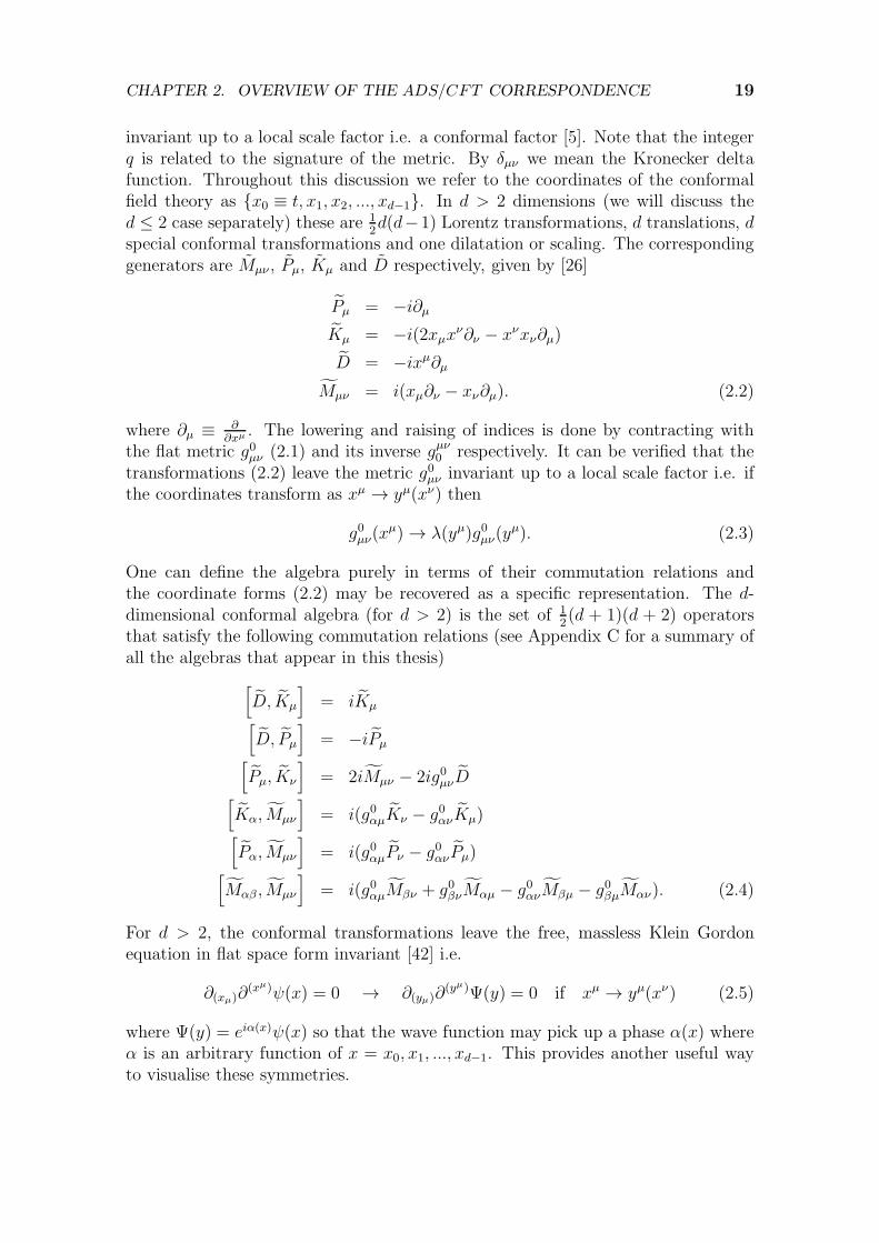
invariant up to a local scale factor i.e. a conformal factor [5]. Note that the integerq is related to the signature of the metric. By δµν we mean the Kronecker deltafunction. Throughout this discussion we refer to the coordinates of the conformalfield theory as x0 ≡ t, x1, x2, ..., xd−1. In d > 2 dimensions (we will discuss thed ≤ 2 case separately) these are 1
2d(d−1) Lorentz transformations, d translations, d
special conformal transformations and one dilatation or scaling. The correspondinggenerators are Mµν , Pµ, Kµ and D respectively, given by [26]
Pµ = −i∂µKµ = −i(2xµxν∂ν − xνxν∂µ)
D = −ixµ∂µMµν = i(xµ∂ν − xν∂µ). (2.2)
where ∂µ ≡ ∂∂xµ . The lowering and raising of indices is done by contracting with
the flat metric g0µν (2.1) and its inverse gµν0 respectively. It can be verified that thetransformations (2.2) leave the metric g0µν invariant up to a local scale factor i.e. ifthe coordinates transform as xµ → yµ(xν) then
g0µν(xµ) → λ(yµ)g0µν(y
µ). (2.3)
One can define the algebra purely in terms of their commutation relations andthe coordinate forms (2.2) may be recovered as a specific representation. The d-dimensional conformal algebra (for d > 2) is the set of 1
2(d + 1)(d + 2) operators
that satisfy the following commutation relations (see Appendix C for a summary ofall the algebras that appear in this thesis)
[D, Kµ
]= iKµ
[D, Pµ
]= −iPµ
[Pµ, Kν
]= 2iMµν − 2ig0µνD
[Kα, Mµν
]= i(g0αµKν − g0ανKµ)
[Pα, Mµν
]= i(g0αµPν − g0ανPµ)
[Mαβ , Mµν
]= i(g0αµMβν + g0βνMαµ − g0ανMβµ − g0βµMαν). (2.4)
For d > 2, the conformal transformations leave the free, massless Klein Gordonequation in flat space form invariant [42] i.e.
∂(xµ)∂(xµ)ψ(x) = 0 → ∂(yµ)∂
(yµ)Ψ(y) = 0 if xµ → yµ(xν) (2.5)
where Ψ(y) = eiα(x)ψ(x) so that the wave function may pick up a phase α(x) whereα is an arbitrary function of x = x0, x1, ..., xd−1. This provides another useful wayto visualise these symmetries.

CHAPTER 2. OVERVIEW OF THE ADS/CFT CORRESPONDENCE 20
2.1.2 CFT Correlation Functions
The requirement of conformal symmetry for a field theory places significant restric-tions on the form of the correlation functions [25], [26]
〈0CFT |O1(t1, ~x1)O2(t2, ~x2)...On(tn, ~xn)|0CFT 〉 (2.6)
whereOm(t, ~x) ≡ eitH Om(~x) e
−itH (2.7)
and |0CFT 〉 refers to the conformal field theory vacuum. The operator Om(~x) hasspatial dependence. By H we mean P0 for the case of conformal field theory butwe make the distinction to allow generalisations (of the time evolution operator).A basis for the enveloping conformal algebra are those operators of definite scalingdimension, O∆, which we define by [5]
[D, O∆(0,~0)] = −i∆O∆(0,~0) (2.8)
where ∆ is the scaling dimension. We may simplify this even further by only con-sidering the primary operators defined by [5]
O∆(0,~0) ∈O∆(0,~0)
such that [O∆(0,~0), Kµ] = 0. (2.9)
This is precisely because the commutator of O∆ with Pµ increases scaling dimensionwhile the commutator with Kµ decrease scaling dimension. The primary operators(2.9) can thus be viewed as the lowest tiers of the ladder of scaling dimension op-erators and one can ladder up by means of differentiation with respect to t andxi from (2.7). The operators obtained by this differentiation process are known asdescendants [5].
The desired quantities from our calculations are thus the 2- and 3-point correla-tion functions of primaries which take a very specific form [27], [28] for CFT s dueto the very restrictive symmetry requirements, namely
〈0CFT |O∆1(t1, ~x1)O∆2
(t2, ~x2)|0CFT 〉
= δ∆1,∆2
2∏
i<j
|ti − tj + |~xi − ~xj ||−(∆i+∆j)
〈0CFT |O∆1(t1, ~x1)O∆2
(t2, ~x2)O∆3(t3, ~x3)|0CFT 〉
= c123
3∏
i<j
|ti − tj + |~xi − ~xj ||∆1+∆2+∆3−2∆i−2∆j1 (2.10)
where the coefficients cijk are dependent on the model under consideration. Thesymbol δ∆1,∆2 again refers to the Kronecker delta function. The coefficients, cijk, ofthree-point functions completely determine the theory since higher point functionsare determined by these [29]. This is by virtue of the operator product expansion[29] where the product of two primary operators at different points may be expressedas the sum of primary operators (and descendants). This allows one to reduce higher
CHAPTER 2. OVERVIEW OF THE ADS/CFT CORRESPONDENCE 21
point functions to a function of the two- and three-point functions.
The AdS/CFT dictionary provides a prescription for calculating these correlationfunctions on the gravity side of the duality. We will present this shortly, but fornow the important point is that the global symmetries of the conformal field theorydetermine the form of the two- and three-point functions (2.10).
2.1.3 AdS Space
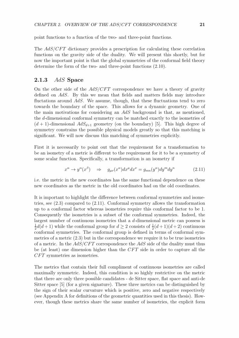
On the other side of the AdS/CFT correspondence we have a theory of gravitydefined on AdS. By this we mean that fields and matters fields may introducefluctations around AdS. We assume, though, that these fluctuations tend to zerotowards the boundary of the space. This allows for a dynamic geometry. One ofthe main motivations for considering an AdS background is that, as mentioned,the d-dimensional conformal symmetry can be matched exactly to the isometries of(d + 1)-dimensional AdSd+1 geometry (on the boundary) [5]. This high degree ofsymmetry constrains the possible physical models greatly so that this matching issignificant. We will now discuss this matching of symmetries explicitly.
First it is necessarily to point out that the requirement for a transformation tobe an isometry of a metric is different to the requirement for it to be a symmetry ofsome scalar function. Specifically, a transformation is an isometry if
xα → yα(xβ) ⇒ gµν(xα)dxµdxν = gmn(y
α)dymdyn (2.11)
i.e. the metric in the new coordinates has the same functional dependence on thesenew coordinates as the metric in the old coordinates had on the old coordinates.
It is important to highlight the difference between conformal symmetries and isome-tries, see (2.3) compared to (2.11). Conformal symmetry allows the transformationup to a conformal factor whereas isometries require this conformal factor to be 1.Consequently the isometries is a subset of the conformal symmetries. Indeed, thelargest number of continuous isometries that a d-dimensional metric can possess is12d(d+1) while the conformal group for d ≥ 2 consists of 1
2(d+1)(d+2) continuous
conformal symmetries. The conformal group is defined in terms of conformal sym-metries of a metric (2.3) but in the correspondence we require it to be true isometriesof a metric. In the AdS/CFT correspondence the AdS side of the duality must thusbe (at least) one dimension higher than the CFT side in order to capture all theCFT symmetries as isometries.
The metrics that contain their full compliment of continuous isometries are calledmaximally symmetric. Indeed, this condition is so highly restrictive on the metricthat there are only three possible candidates - de Sitter space, flat space and anti-deSitter space [5] (for a given signature). These three metrics can be distinguished bythe sign of their scalar curvature which is positive, zero and negative respectively(see Appendix A for definitions of the geometric quantities used in this thesis). How-ever, though these metrics share the same number of isometries, the explicit form

CHAPTER 2. OVERVIEW OF THE ADS/CFT CORRESPONDENCE 22
of these isometries are different.
It is only anti-de Sitter space which contains all the appropriate isometries in thesense that they match the symmetries (2.2) of the conformal group [5]. This exactmatching can be done on the conformal boundary of AdS. A convenient form forthe AdSd+1 metric is the so-called Poincare patch given by
ds2 =L2
β2
(dβ2 + d~x · d~x
)(2.12)
where xα has d components and for which the scalar curvature, RS = − (d+1)(d)L2 , is
constant. Note that while the AdSd+1 metric (2.12) always possesses 12(d+1)(d+2)
isometries, it is only on the β → 0 boundary that the explicit coordinate form ofthese isometries corresponds exactly to the d-dimensional conformal group [5]. Themetric (2.12) is in Euclidean signature. We will be working in Euclidean signaturethroughout this thesis.
2.1.4 The d ≤ 2 Conformal Group
As promised we need to discuss the conformal group for dimension d ≤ 2 separately.We borrow greatly from [25], [26] in this section. We discuss the case where d = 2explicitly, but the case d = 1 is treated in very similar fashion.
As before the conformal group is defined in terms of the transformations thatleave the flat space metric (2.1) invariant up to a conformal factor. We considerthe Euclidean signature flat space metric and transform to complex coordinatesz = x0 + ix1, z = x0 − ix1. We then have
ds2 = g0µνdxµdxν = dzdz. (2.13)
Consider an arbitrary coordinate transformation w = w(z) and the correspondingw = w(z). The metric is transformed to
ds2 =dz
dw
dz
dwdwdw (2.14)
so that it is clear that this arbitrary coordinate transformation is a conformal trans-formation of the metric. The conformal group in two dimensions is thus infinitedimensional. By an almost identical argument one can show that the conformalgroup in one dimension is also infinite dimensional.
A subset of the transformations w = w(z) are of special interest namely
w =αz + β
γz + δ(2.15)
where α, β, γ and δ are complex numbers that satisfy αδ − βγ = 1. These transfor-mations are called the “global conformal transformations” and correspond exactlyto SO(3, 1). This is what we would have gotten if we simply substituted d = 2 in
CHAPTER 2. OVERVIEW OF THE ADS/CFT CORRESPONDENCE 23
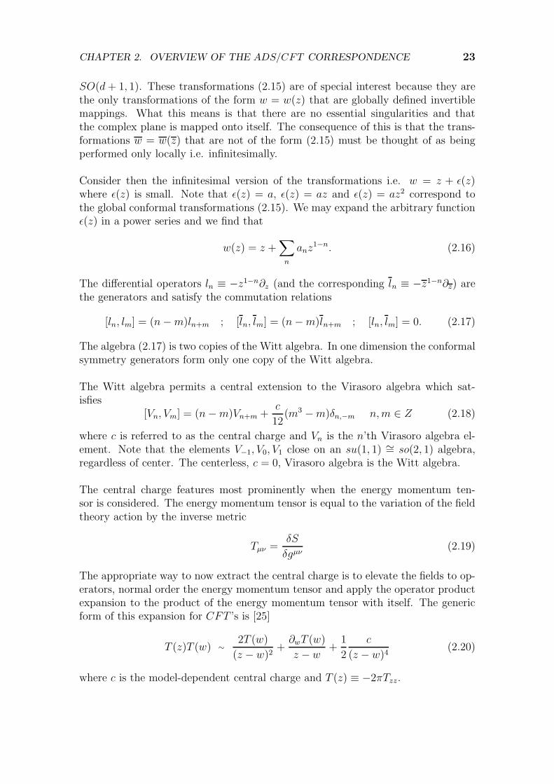
SO(d+ 1, 1). These transformations (2.15) are of special interest because they arethe only transformations of the form w = w(z) that are globally defined invertiblemappings. What this means is that there are no essential singularities and thatthe complex plane is mapped onto itself. The consequence of this is that the trans-formations w = w(z) that are not of the form (2.15) must be thought of as beingperformed only locally i.e. infinitesimally.
Consider then the infinitesimal version of the transformations i.e. w = z + ǫ(z)where ǫ(z) is small. Note that ǫ(z) = a, ǫ(z) = az and ǫ(z) = az2 correspond tothe global conformal transformations (2.15). We may expand the arbitrary functionǫ(z) in a power series and we find that
w(z) = z +∑
n
anz1−n. (2.16)
The differential operators ln ≡ −z1−n∂z (and the corresponding ln ≡ −z1−n∂z) arethe generators and satisfy the commutation relations
[ln, lm] = (n−m)ln+m ; [ln, lm] = (n−m)ln+m ; [ln, lm] = 0. (2.17)
The algebra (2.17) is two copies of the Witt algebra. In one dimension the conformalsymmetry generators form only one copy of the Witt algebra.
The Witt algebra permits a central extension to the Virasoro algebra which sat-isfies
[Vn, Vm] = (n−m)Vn+m +c
12(m3 −m)δn,−m n,m ∈ Z (2.18)
where c is referred to as the central charge and Vn is the n’th Virasoro algebra el-ement. Note that the elements V−1, V0, V1 close on an su(1, 1) ∼= so(2, 1) algebra,regardless of center. The centerless, c = 0, Virasoro algebra is the Witt algebra.
The central charge features most prominently when the energy momentum ten-sor is considered. The energy momentum tensor is equal to the variation of the fieldtheory action by the inverse metric
Tµν =δS
δgµν(2.19)
The appropriate way to now extract the central charge is to elevate the fields to op-erators, normal order the energy momentum tensor and apply the operator productexpansion to the product of the energy momentum tensor with itself. The genericform of this expansion for CFT ’s is [25]
T (z)T (w) ∼2T (w)
(z − w)2+∂wT (w)
z − w+
1
2
c
(z − w)4(2.20)
where c is the model-dependent central charge and T (z) ≡ −2πTzz.

CHAPTER 2. OVERVIEW OF THE ADS/CFT CORRESPONDENCE 24
We take note of an important consequences of (2.20) and the conformal Ward iden-tity [25] applied to the energy momentum tensor
δǫT (w) = − 1
2πi
∮
C
dwǫ(z)T (z)T (w). (2.21)
The expression (2.21) calculates the change of T (z) under a shift z → z + ǫ(z).The contour integral picks up the residues of the integrand. Substituting (2.20) into(2.21) yields
T (z) → T (z)− ǫ(z)∂zT (z)− 2∂zǫ(z)T (z)−c
12∂3z ǫ(z). (2.22)
The finite version of the transformation (2.22), where w = w(z) is given by
T (w) =
(dw
dz
)−2 [T (z)− c
12w; z
](2.23)
where w; z is the Schwarzian derivative
w; z = ∂z
(d2wdz2
dwdz
)− 1
2
(d2wdz2
dwdz
)2
. (2.24)
We will use the transformation property (2.23) in section 4.5 to identify a centralcharge of a one-dimensional conformal field theory.
2.2 Correlation Functions From Generating
Functionals
Now that we have discussed the symmetries in some detail we turn our attention tohow correlation functions are calculated in the field theory and, through the use ofthe dictionary, in the gravitational dual.
We specify the coordinates of the CFTd as x0 ≡ t, x1, x2, ..., xd−1 which is matchedwith the boundary of AdSd+1. The gauge/gravity dictionary provides a very partic-ular prescription [3], [5], [6], [30] for calculating correlation functions (2.10) in whichthe generating functional
ZCFT [φ∆i] = 〈0QFT | exp
∫ddx
∑
i
φ∆i(x)O∆i
(x)
|0QFT 〉 (2.25)
features prominently. The correlation functions (2.10) can be found by taking appro-priate functional derivatives of the generating functional (2.25) with respect to thesources φ∆i
(xi) and afterwards setting the sources to zero. The operators O∆iare
primary operators, as discussed in section 2.1.2. The generating functional (2.25)thus represents the single quantity one needs to compute in order to find the quan-tities of interest, the correlation functions.
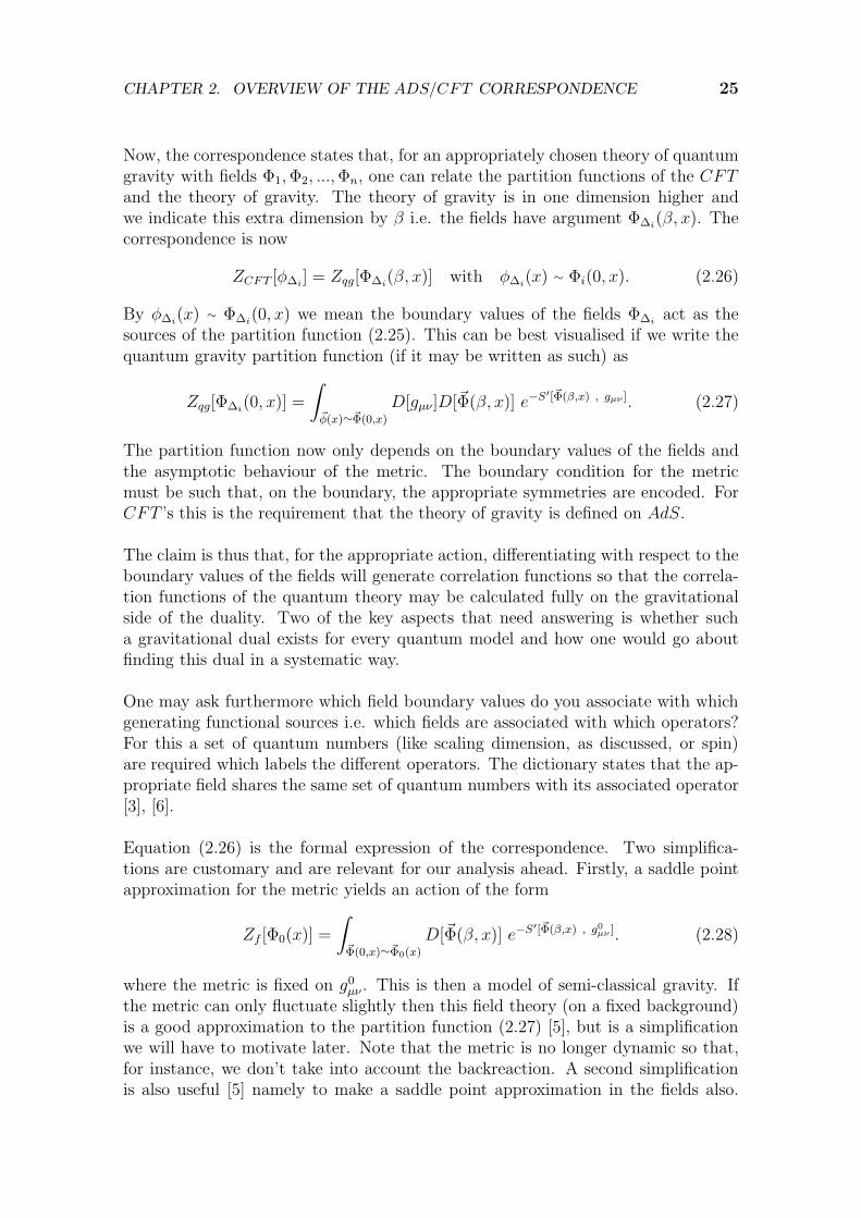
CHAPTER 2. OVERVIEW OF THE ADS/CFT CORRESPONDENCE 25
Now, the correspondence states that, for an appropriately chosen theory of quantumgravity with fields Φ1,Φ2, ...,Φn, one can relate the partition functions of the CFTand the theory of gravity. The theory of gravity is in one dimension higher andwe indicate this extra dimension by β i.e. the fields have argument Φ∆i
(β, x). Thecorrespondence is now
ZCFT [φ∆i] = Zqg[Φ∆i
(β, x)] with φ∆i(x) ∼ Φi(0, x). (2.26)
By φ∆i(x) ∼ Φ∆i
(0, x) we mean the boundary values of the fields Φ∆iact as the
sources of the partition function (2.25). This can be best visualised if we write thequantum gravity partition function (if it may be written as such) as
Zqg[Φ∆i(0, x)] =
∫
~φ(x)∼~Φ(0,x)
D[gµν ]D[~Φ(β, x)] e−S′[~Φ(β,x) , gµν ]. (2.27)
The partition function now only depends on the boundary values of the fields andthe asymptotic behaviour of the metric. The boundary condition for the metricmust be such that, on the boundary, the appropriate symmetries are encoded. ForCFT ’s this is the requirement that the theory of gravity is defined on AdS.
The claim is thus that, for the appropriate action, differentiating with respect to theboundary values of the fields will generate correlation functions so that the correla-tion functions of the quantum theory may be calculated fully on the gravitationalside of the duality. Two of the key aspects that need answering is whether sucha gravitational dual exists for every quantum model and how one would go aboutfinding this dual in a systematic way.
One may ask furthermore which field boundary values do you associate with whichgenerating functional sources i.e. which fields are associated with which operators?For this a set of quantum numbers (like scaling dimension, as discussed, or spin)are required which labels the different operators. The dictionary states that the ap-propriate field shares the same set of quantum numbers with its associated operator[3], [6].
Equation (2.26) is the formal expression of the correspondence. Two simplifica-tions are customary and are relevant for our analysis ahead. Firstly, a saddle pointapproximation for the metric yields an action of the form
Zf [Φ0(x)] =
∫
~Φ(0,x)∼~Φ0(x)
D[~Φ(β, x)] e−S′[~Φ(β,x) , g0µν ]. (2.28)
where the metric is fixed on g0µν . This is then a model of semi-classical gravity. Ifthe metric can only fluctuate slightly then this field theory (on a fixed background)is a good approximation to the partition function (2.27) [5], but is a simplificationwe will have to motivate later. Note that the metric is no longer dynamic so that,for instance, we don’t take into account the backreaction. A second simplificationis also useful [5] namely to make a saddle point approximation in the fields also.

CHAPTER 2. OVERVIEW OF THE ADS/CFT CORRESPONDENCE 26
Varying the action with respect to the fields yields a differential equation for thefields ~Φ of which the solutions are ~Φcl i.e.
δS
δ~Φ
∣∣∣∣~Φ=~Φcl
= 0 (2.29)
The correspondence then becomes
ZCFT [φ(x)] ≈ Zcl−qg[φ(x)] =∑
~Φcl
e−S[Φcl] (2.30)
where we mean∑
~Φclto be a sum over all the possible solutions of (2.29). In this
notation it is slightly more hidden, but the generating functional is still determinedby the boundary values for the fields (only now their classical solutions).
2.3 Local / Gauge Symmetries
The discussion of the previous sections may be viewed as the most basic outline ofthe correspondence and we have not yet in any way specified how the gravitationaltheory may be chosen. In order to discuss further aspects of the correspondence wehave to consider more specifics of conformal field theories.
In the Maldacena correspondence [1] there is, in addition to the conformal globalsymmetry, also the SU(N) gauge symmetry on the CFT side of the duality. This isa matter we have not addressed yet precisely because gauge symmetry will not be afeature of our ensuing construction. This aspect is, however, very important both asevidence for the duality as well as for the role played by the gauge group dimensionN in defining the strong and weak coupling regimes. Future generalisations of ourconstruction that include these local symmetries are thus very important.
A local transformation, when represented as a unitary operator means U = eiα(t,~x)T
where T is the generator 2. Note that, unlike a global symmetry, the coefficient αis now a function of the coordinates. To best illustrate this difference consider thefollowing action density
L(φ, φ†) = ∂µφ† ∂µφ (2.31)
with matrix valued fields φ. Global transformations, where φ→ Uφ and φ† → φ†U †
leave L invariant. Local transformations, on the other hand, are affected by thederivative and L will thus not retain its form. In order to allow local transformationsone needs to augment L and consider
L′(φ, φ†, Aµ) = (∂µ + iAµ)φ†(∂µ − iAµ)φ. (2.32)
Local transformations can now be included as a symmetry if the Aµ’s transform as
Aµ → UAµU† − iU †∂µU. (2.33)
2We assume that the operator U is well-defined as it illustrates the gauge transformations moreclearly. If not, then our notation means the infinitesimal version of these transformations.
CHAPTER 2. OVERVIEW OF THE ADS/CFT CORRESPONDENCE 27
A distinguishing property of the global and local transformations thus is that globaltransformations affect the quantum states or fields only while the local transfor-mations affect the states but also the gauge. This observation fits well with ourconstruction that will be made in chapter 3 - the geometry is constructed from thequantum states and thus can only take note of the global symmetries.
It is useful (and quite typical) to consider these theories in the fundamental rep-resentation i.e. the N × N matrix representation of the gauge group SU(N). Invector valued theories, such as higher spin [31], the fields φ then represent N -indexvectors and the inner product φ†φ′ is simply the dot product while in matrix-valuedtheories (such as SYM) the fields are N ×N matrices with the trace inner product.The usefulness of this representation is that the N -dependence of the inner productof fields becomes explicit.
It was shown by t’Hooft [11] and Witten [12] that gauge theories permit a 1N
expan-sion for the (many-point) correlators, with each term in this expansion correspondingto a class of diagrams that have a specific topological character. The Feynman di-agrams of the leading order terms, for instance, are planar i.e. they can be drawnwithout crossings on the surface of a sphere. The next leading order term can bedrawn on a 1-torus (a torus with a single hole), the next on a 2-torus et cetera.These results are remarkable since one may intuitively expect that increasing Nadds complexity to the problem - somehow the converse is true and the theory canbe rearranged so that it is in fact simpler in this large N expansion.
This classification scheme and particularly its topological character, is reminiscentof Feynman diagrams for string theory and thus a hint that these gauge theories maybe described by string theories [5]. The expansion parameter 1
Nof the topological
series is crucial to the convergence properties of this series. For the Maldacena caseof Super Yang-Mills, for instance, the limit needs to be taken in a very specific way[1]. The t’Hooft limit is N → ∞ and gYM → 0 while keeping λ ≡ g2YMN constant.The constant λ is called the t’Hooft coupling and gYM is the Yang-Mills coupling.This limit permits the large N topological expansion of the gauge theory.
2.3.1 The Maldacena Correspondence
In [1] the relevant parameters on the side of the of the N = 4 SYM are the dimen-sion of the gauge group N and the Yang-Mills coupling gYM . On the gravity side therelevant constants are the string coupling, gs and the string length ls. The other pa-rameters, such as the AdS radius, L, forms part of the geometry as already discussed.
The Maldacena conjecture relates these quantities explicitly [5], [6]
g2YM = gs
λ =L4
l4s(2.34)
or alternatively, using the relation between the string scale, Planck scale and thecoupling
CHAPTER 2. OVERVIEW OF THE ADS/CFT CORRESPONDENCE 28
gs =(ls)4
(lp)4, we find
N =L4
l4p. (2.35)
These conjectured relations between the two theories provide a powerful insight.Firstly, the conformal field theory can be solved perturbatively if the t’Hooft cou-pling, λ is small. Conversely the string length is much larger than the length scaleof the AdS space from eq. (2.34). The string theory on the AdS background isconsequently hard to analyse. Conversely, if N is large we have that the AdS radiusis large compared to the Planck scale from eq. (2.35). This implies that quantumeffects will play a small role in the string theory so that we may consider a modelof semi-classical gravity. Note that this holds for any value of the string coupling gsso that we have not specified the t’Hooft coupling.
In other words, the strongly coupled string theory may be described by a weaklycoupled field theory and the field theory for large N may be described by semi-classical gravity. This is a so-called strong/weak duality and it promotes the dualityto a powerful tool to calculate physical quantities in the strongly coupled regime.
For our purposes we take note of the fact that there exists a limit in which thegauge theory can be accurately described by a semi-classical model of gravity. Inthe analysis ahead we will be working with semi-classical gravity since it is thesimplest case.
2.4 Summary
There are many aspects of holography that have been omitted and may be consid-ered in future generalisations. The aim of this chapter was simply to illuminatesome essential aspects of the foundation of the gauge/gravity duality. The role ofsymmetries as the core of the correspondence was highlighted along with intuitivearguments for how a quantum theory may be repackaged as a theory of gravitation.
The dictionary of the Maldacena correspondence [1] was stated and particular notemust be taken of the role of the boundary values of fields acting as sources. It shouldbe noted that the dictionary we will construct in the chapters that follow will notattach this interpretation to the fields of the gravitational model. For our purposesthere is a simpler choice that can be made (and one that relates remarkably wellto existing work in the literature). We will point out exactly where this choice ofinterpretation is made in the procedure so that one may in future investigate otherpossibilities.
The simplification from conformal field theory to quantum mechanics will comeat a price - we will not be working with gauge theories and will thus apparently lacka large N expansion. We acknowledge that incorporating gauge symmetry is a layerof complexity that warrants an extensive look in future.

CHAPTER 2. OVERVIEW OF THE ADS/CFT CORRESPONDENCE 29
We will show, in the chapters ahead, that this simplification does yield great value inthat it is possible to build dual descriptions of quantum mechanical models system-atically and explicitly. This will allow us to investigate the dictionary for the dualtheories in a very direct way and we will show how many existing results, especiallyof the AdS2/CFT1 correspondence, come about very naturally from this systematicmachinery.
Chapter 3
Constructing Metrics FromQuantum States
We will be constructing geometries from quantum mechanical models as a first stepto finding a systematic, constructive and efficient way to repackage these quantummodels as gravitational theories. We choose this geometric perspective for severalreasons. The matching of (global) symmetries between gauge theories and theories ofgravity is one of the main motivations for conjecturing the existence of gauge/gravitydualities. In numerous works examining candidate duals for quantum mechanicalmodels [13], [20], [21], [33], [34] a metric possessing the appropriate isometries istaken as a starting point for investigations. If the symmetries of the two modelsmatch, and the sets of symmetries are large (and thus restrictive) enough, then, atleast in this sense, a significant part of the dual matching is done. Not only can aprocedure be devised that guarantees that the appropriate symmetries of a quantummodel are encoded as isometries of a geometric structure but this procedure can besystematic and explicit.
As a study of the literature will point out [14], [32], [35], [36], [37], [38], [39], [40],there are, in fact, many ways to construct geometries from quantum models. It isthus of critical importance that a sensible choice of geometry is made. In [14] itwas shown that appropriate geometric structures allow a given quantum mechanicalmodel to be reformulated entirely in terms of these structures. This aspect has tobe treated with some care - what quantum mechanical quantities can we calculatefrom our dual description? Is knowledge of the geometry sufficient to calculate thequantities of interest and, if so, how does one do this? If not, what is needed inaddition to the geometry?
In this chapter we will introduce the construction of a metric and anti-symmetrictwo-form that we will use throughout this thesis. We will give some motivations forwhy this construction is chosen. We elaborate briefly on other intriguing construc-tions that can be investigated in future.
30

CHAPTER 3. CONSTRUCTING METRICS FROM QUANTUM STATES 31
3.1 Dynamical Symmetries
Before we present the construction it is important to clarify what is meant by asymmetry of a set of quantum mechanical states as these states are our startingpoint. The terminology we will be using is that of dynamical symmetries [41], [42]which can also be found in the literature under the name of the kinematical invari-ance group [43], [44]. As far as this author can tell these names refer to the samesymmetries.
Throughout this thesis we will use the notation |·〉 for normalised kets and |·) forkets that aren’t necessarily normalised. Now, consider a family of states labelled bya set of coordinates ~α which may or may not be real. If there exists a unitary trans-formation, Ug whose action on the states can be absorbed as a reparametrisationand normalisation of the states |~α) i.e.
Ug|~α) = [fg(~α)]−1|g(~α)) (3.1)
then the transformation ~α → g(~α) is what we will call a dynamical symmetry ofthe states. The motivation for this terminology will be more apparent in the nextsection. Note that if the states are normalised in (3.1) then the normalisation factorfg(~α) will simply be a phase. Since we will be working with both normalised andunnormalised states we keep it as a general normalisation factor.
One may ask why start with the symmetries of quantum states and not, for in-stance, the symmetries of a Lagrangian or action. The reason for this will becomeapparent in section 4.7. The transformation properties of the quantum states underunitary transformations will allow us to speak to the properties of state overlaps andexpectation values. These are, for this thesis, the quantum mechanical analogue ofcorrelation functions.
3.1.1 The Schrodinger Equation as a Specific Example of
Dynamical Symmetries
The dynamical symmetries are often discussed [43], [44] on the level of the time-dependent Schrodinger equation. We would like to stress that, though instructive,this is a specific example of the definition (3.1).
The dynamical symmetries may be visualised, if applicable to the problem underconsideration, as the transformations that leave the time-dependent Schrodingerequation invariant up to a scale factor i.e. there is a transformation x, t →x′(x, t), t′(x, t) such that
0 = i∂
∂tψ(t, x) +
1
2∇2ψ(t, x)− V (x)ψ(t, x)
→ 0 = i∂
∂t′Ψ(t′, x′) +
1
2∇′2Ψ(t′, x′)− V (x′)Ψ(t′, x′) (3.2)
where Ψ(t′(t, x), x′(t, x)) = f(t, x)ψ(t, x) with f(t, x) some scalar function. We havechosen units such that ~ = 1 and m = 1.

CHAPTER 3. CONSTRUCTING METRICS FROM QUANTUM STATES 32
We can recast the symmetries of (3.2) into the form of definition (3.1) by rewritingthe wave function in bra-ket notation. The conjugate of the wave function is givenby
ψ∗(t, x) = 〈ψ|t, x) ; where |t, x) = eitHeixP |x = 0). (3.3)
The dynamical symmetries, applying definition (3.1), are associated with unitarytransformations Ug|x, t) = [fg(t, x)]
−1|g(t, x)). The dynamical symmetries thus leavethe propagator unchanged up to a normalisation of the states
(x′, t′|x, t) = (x′, t′|U †gUg|x, t) = [fg(t, x)]
−1[f ∗g (t
′, x′)]−1(g(t′, x′)|g(t, x)) (3.4)
but not necessarily the wavefunction.
3.1.2 The Dynamical Symmetries of the Free Particle
An important and illustrative example of dynamical symmetries is that of the freeparticle [43]. The dynamical symmetry generators of the free Schrodinger equationin 1+1 dimensions ((3.2) with V (x) = 0) closes on the 1+1 dimensional Schrodingeralgebra schr1+1. The algebra can be represented in many different ways - for instanceas creation and annihilation operators [45] or 4× 4 matrices [46]. For the purposesof this thesis we will represent them in terms of position and momentum operators
I = −i(XP − PX)
H =1
2P 2
D = −1
4(XP + PX)
K =1
2X2 (3.5)
along with position, X , and momentum, P . The operators H,D,K (3.5) are in thek = 1
4irrep of su(1, 1). See Appendix C for more detail. The schr1+1 algebra closes
on the following set of commutation relations
[X,P ] = −i ; [K,H ] = −2iD
[P,D] =i
2P ; [X,D] = − i
2X
[P,K] = iX ; [X,H ] = −iP[K,D] = −iK ; [H,D] = iH
0 otherwise (3.6)
and is the semi-direct sum of su(1, 1) (spanned by H,D,K) and the Heisenbergalgebra (spanned by P,X, I). These operators derive their names from the coor-dinate transformation induced on the free particle states, |t, x) ≡ eitHeixP |x = 0),

CHAPTER 3. CONSTRUCTING METRICS FROM QUANTUM STATES 33
namely
eiaH |t, x) = |t+ a, x)
eiaP |t, x) = |t, x+ a)
eiaD|t, x) = ea2 |eat, ea
2x)
eiaX |t, x) = eiax+ia2t|t, x+ 2at)
eiaK |t, x) = eiαx2
2(1−αt) (1− at)−12
∣∣∣∣t
1− at,
x
1− at
)(3.7)
which is time translation, space translation, scaling, Galilean boost and special con-formal transformations respectively. These transformations can be calculated usingthe BCH formulas outlined in appendix D. The special conformal transformation of(3.7) is shown explicitly in (D.22).
A comment here is in order. The reader may pick up that the operators (3.6)do not have an explicit time dependence while the generators of dynamical symme-try in [43] do. The time and spatial dependence of the operators come about whenthey act on the state |t, x). Their action on the state can be viewed as a differentialoperator where H represents a time-derivative and P represents a spatial derivative.Of course, the time-dependent operators e−itHUeitH are also symmetry generatorsof the state |t, x).
We can verify (3.4) by explicitly applying the transformations (3.7) to the 1 + 1dimensional free particle propagator
(t′, x′|t, x) = (2πi(t− t′))−12 e
− (x−x′)2
2i(t−t′) . (3.8)
As a final comment, if we restrict ourselves to the free particle symmetries thatinvolve time, H,D,K from eq. (3.7), we explicitly have the su(1, 1) ∼= so(2, 1)algebra. In section 2.1.3 we identified the SO(2, 1) group as the isometry groupof AdS2 (2.1) so that, if the metric we construct encodes dynamical symmetries asisometries, one may anticipate that the geometry will be AdS2.
3.2 The Construction of our Metric and
Anti-symmetric Two-Form
The construction we will be employing in this thesis is the metric [47] as studiedby Provost and Vallee [36]. This metric is closely related to the work of [14], [35]which will be the topic of section 3.3. We will show explicitly that this constructioncan be used to encode the dynamical symmetries of a family of quantum states asisometries of the resulting metric (3.1). We will specifically be considering statesthat are parametrised by continuous coordinates. This may seem strange at firstsight since in quantum mechanics one typically considers states that are labelled bydiscrete quantum numbers. The states of continuous parameters must be viewed assuperpositions of these states of discrete quantum numbers where the superposition

CHAPTER 3. CONSTRUCTING METRICS FROM QUANTUM STATES 34
coefficients are continuous.
We begin by defining the metric [36] which will be used in the ensuing construction.We define it here for an arbitrary family of states and we will apply it to specificphysical situations later. Let |s〉 be a manifold of normalized states parametrizedby a set of real coordinates s = (s1, s2, s3, . . .). As mentioned we use |s) to denote astate proportional to |s〉 which need not be normalized. In the construction we set
βj(s) = −i∂j′ 〈s|s′〉 |s=s′ and γij(s) + iσij(s) = ∂i∂j′ 〈s|s′〉 |s=s′, (3.9)
where γij = γji and σij = −σji are related to the real and imaginary parts of theinner product
(〈s+ dsi| − 〈s|)(|~s+ dsj〉 − |~s〉). (3.10)
By s+ dsi we mean an infinitesimal shift in si. The metric [36] is then defined as
gij(s) = γij(s)− βi(s)βj(s), (3.11)
which may be rewritten as
gij(s) = [ ∂i∂j′ log |(s|s′)| ]s=s′. (3.12)
The definitions (3.11) and (3.12) are completely equivalent. The subtraction of theβiβj combination in (3.11) ensures that the distance between state vectors that onlydiffer by a phase is zero i.e. the metric (3.12) can be thought of as a “distance” be-tween physical states. We can thus refer to the metric and anti-symmetric two-formas being defined on the manifold of rays. In other words state vectors that differ bya phase factor (or normalisation) are represented by the same point on the manifold.This can also be seen in (3.12) which has an additional useful property - the metricis no longer sensitive to whether the states are normalised. Note, importantly, thatin the definition (3.12) we have the freedom to use either the normalised or unnor-malised states to calculate the metric.
A similar formula to (3.12) exists for the anti-symmetric two-form σij (3.9) namely
σij =1
2i[ ∂i∂j
′ log(s|s′)(s′|s) ]s=s′. (3.13)
A Quick Example
As an example of calculating the metric and anti-symmetric two-form consider theapplication of (3.12) and (3.13) on the free particle overlap (3.8). We have that
log(t′, x′|t, x) = −1
2log(2πi)− 1
2log(t− t′)− (x− x′)2
2i(t− t′). (3.14)
If we apply the formulae (3.12) and (3.13) directly the metric and two-form willclearly be divergent when we try to set x′ = x and t′ = t. A way to rectify this is tocomplexify the coordinates (we will employ regularisation schemes throughout whenthese situations arise). We thus alter t→ t+ iβ and the corresponding t′ → t′ − iβ
CHAPTER 3. CONSTRUCTING METRICS FROM QUANTUM STATES 35
on the right hand side of (3.14). The reason for the different sign is the conjugationinvolved when considering bras vs. kets.
These changes yield
log(t′ + iβ ′, x′|t+ iβ, x)
= −1
2log(2πi)− 1
2log(t− t′ + i(β + β ′))− (x− x′)2
2i(t− t′ + i(β + β ′)).
One can now readily calculate
∂t∂t′ log(t′ + iβ ′, x′|t+ iβ, x) = − 1
2(t− t′ + i(β + β ′))2− i(x− x′)2
(t− t′ + i(β + β ′))3
= ∂β∂β′ log(t′ + iβ ′, x′|t+ iβ, x)
∂t∂β′ log(t′ + iβ ′, x′|t+ iβ, x) =i
2(t− t′ + i(β + β ′))2− (x− x′)2
(t− t′ + i(β + β ′))3
= −∂β∂t′ log(t′ + iβ ′, x′|t+ iβ, x)
∂x∂x′ log(t′ + iβ ′, x′|t+ iβ, x) = − i
t− t′ + i(β + β ′). (3.15)
The remaining derivatives are omitted since they will yield entries that are zero.From the above expressions we find
gtt = gββ =1
8β2
gxx = − 1
2β. (3.16)
The non-zero entries for the β, t derivatives do not reflect in the metric becausethey are anti-symmetric. They do, however, feature in the anti-symmetric two-form
σβt = −σtβ =1
8β2(3.17)
3.2.1 Dynamical Symmetries and Isometries
The construction is chosen precisely because it encodes the dynamical symmetries ofa family of states as the isometries of a metric. Consider a unitary transformationUg which produces a mapping s → g(s) on the manifold |s〉 as in (3.1). Thetransformation constitutes a dynamical symmetry as discussed. In particular, thisimplies that
〈g(s)|g(s′)〉 = 〈s|s′〉 f ∗g (s)fg(s
′). (3.18)
Now consider s → u(s) as a coordinate transformation and let t = u(s) denote thenew coordinates. Inserting 〈s|s′〉 = 〈t|t′〉 [f ∗
g (s)fg(s′)]−1 into eq. (3.12) reveals that
gij(s) = [ ∂si∂s′j log | 〈t|t′〉 | ]s=s′ =
∂uk∂si
∂ul∂sj
[ ∂uk∂u′
llog | 〈t|t′〉 | ]t=t′ =
∂uk∂si
∂ul∂sj
gkl(t)
(3.19)
CHAPTER 3. CONSTRUCTING METRICS FROM QUANTUM STATES 36
and thus
ds2 = gij(s)dsidsj = gkl(t)∂tk∂si
∂tl∂sj
dsidsj = gkl(t)dtkdtl. (3.20)
We conclude that the mapping s→ g(s) is an isometry of the metric.
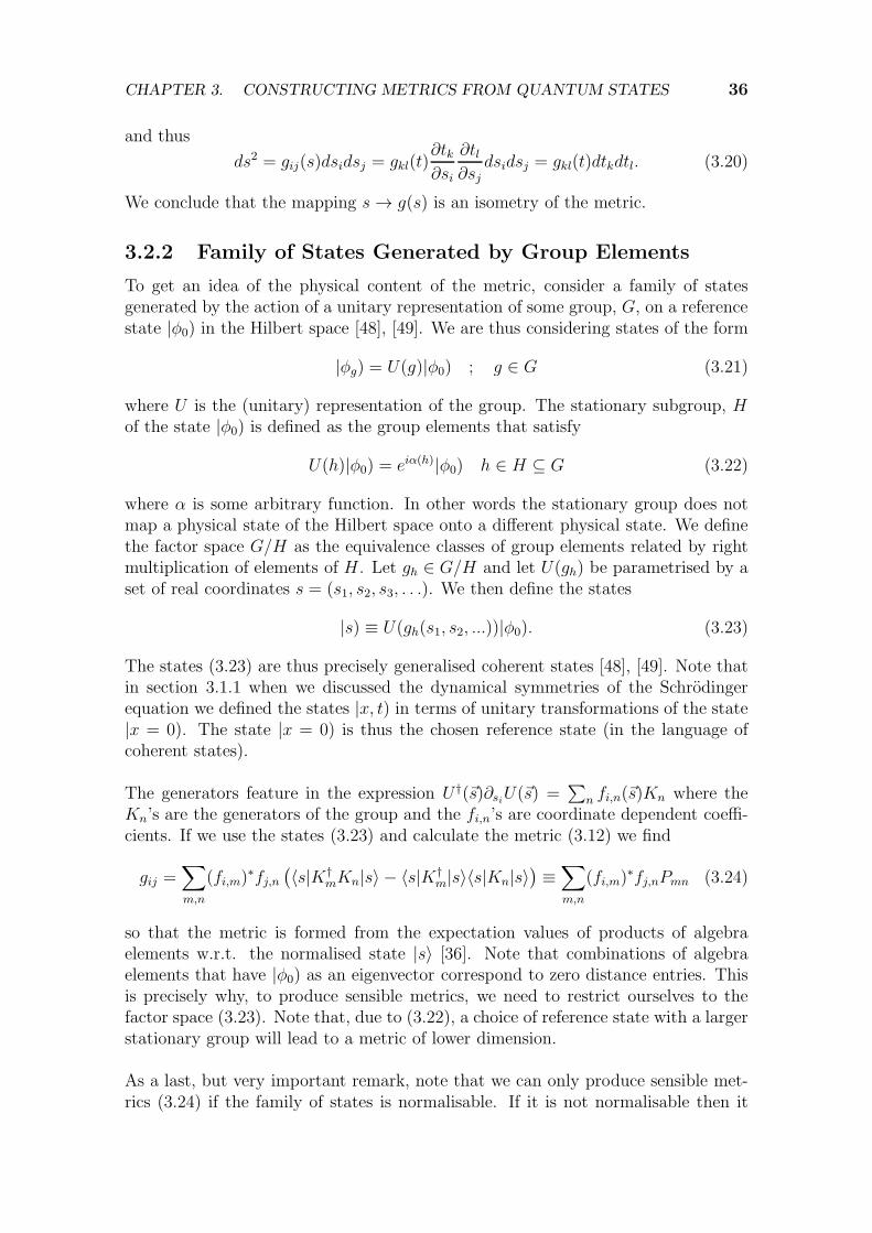
3.2.2 Family of States Generated by Group Elements
To get an idea of the physical content of the metric, consider a family of statesgenerated by the action of a unitary representation of some group, G, on a referencestate |φ0) in the Hilbert space [48], [49]. We are thus considering states of the form
|φg) = U(g)|φ0) ; g ∈ G (3.21)
where U is the (unitary) representation of the group. The stationary subgroup, Hof the state |φ0) is defined as the group elements that satisfy
U(h)|φ0) = eiα(h)|φ0) h ∈ H ⊆ G (3.22)
where α is some arbitrary function. In other words the stationary group does notmap a physical state of the Hilbert space onto a different physical state. We definethe factor space G/H as the equivalence classes of group elements related by rightmultiplication of elements of H . Let gh ∈ G/H and let U(gh) be parametrised by aset of real coordinates s = (s1, s2, s3, . . .). We then define the states
|s) ≡ U(gh(s1, s2, ...))|φ0). (3.23)
The states (3.23) are thus precisely generalised coherent states [48], [49]. Note thatin section 3.1.1 when we discussed the dynamical symmetries of the Schrodingerequation we defined the states |x, t) in terms of unitary transformations of the state|x = 0). The state |x = 0) is thus the chosen reference state (in the language ofcoherent states).
The generators feature in the expression U †(~s)∂siU(~s) =∑
n fi,n(~s)Kn where theKn’s are the generators of the group and the fi,n’s are coordinate dependent coeffi-cients. If we use the states (3.23) and calculate the metric (3.12) we find
gij =∑
m,n
(fi,m)∗fj,n
(〈s|K†
mKn|s〉 − 〈s|K†m|s〉〈s|Kn|s〉
)≡∑
m,n
(fi,m)∗fj,nPmn (3.24)
so that the metric is formed from the expectation values of products of algebraelements w.r.t. the normalised state |s〉 [36]. Note that combinations of algebraelements that have |φ0) as an eigenvector correspond to zero distance entries. Thisis precisely why, to produce sensible metrics, we need to restrict ourselves to thefactor space (3.23). Note that, due to (3.22), a choice of reference state with a largerstationary group will lead to a metric of lower dimension.
As a last, but very important remark, note that we can only produce sensible met-rics (3.24) if the family of states is normalisable. If it is not normalisable then it

CHAPTER 3. CONSTRUCTING METRICS FROM QUANTUM STATES 37
will be essential to regularise the reference state i.e. we require a family of states|φ0(~β)), parametrised by real coordinates ~β = (β1, β2, ...), so that (φ0(~β)|φ0(~β)) <∞for some domain of ~β and |φ0(~0)) = |φ0). This regularisation will almost certainlybreak (some of) the symmetries of the family of states but these are recovered on
the ~β → ~0 boundary, where the original family of states are defined. We interpretthese regularisation parameters as bulk coordinates so that we have a clear “bulk”and “boundary” region. For the examples that we will be considering it is possibleto choose the regularisation in such a way that all the symmetries are retained asisometries in the bulk.
3.3 The Geometric Reformulation of Quantum
Mechanics
Thus far we have identified the construction (3.12) which encodes the dynamicalsymmetries of a set of quantum states as isometries of a metric, whilst being arelatively straightforward calculation. These features make the construction an ap-pealing first step towards building dual descriptions. We will now point out that thismetric and anti-symmetric two-form (3.12) is related to the geometric reformulationof quantum mechanics of Ashtekar and Schilling [14], [35].
First, some context is necessary. This geometric reformulation of quantum me-chanics starts from an interesting premise: can quantum mechanics be formulatedentirely in terms of measurable quantities? In other words, can quantum mechanicsbe formulated entirely in terms of the projective Hilbert space? The result to theensuing analysis is a geometric reformulation of quantum mechanics. For our pur-poses the precise form of, for instance, the postulates of quantum mechanics in thisreformulation are unimportant (these can all be found in [14], [35]).
We will here only give a brief summary of the aspects that will be important for ourpurposes. We borrow their notation almost identically. Their conventions for sym-plectic geometry is that the Hamiltonian vector field Xf , generated by the functionf satisfies iXf
Ω = df , where Ω is the symplectic form.
The starting point of the reformulation [14] is to take a complex Hilbert spaceand decompose it into its real and imaginary parts. In terms of the inner productof two arbitrary states in the Hilbert space |ψ), |φ) this is
(φ|ψ) = Re((φ|ψ)) + i Im((φ|ψ))≡ 1
2G(φ, ψ) +
i
2Ω(φ, ψ). (3.25)
The properties of the inner product imply that G is positive definite and that Ω isa symplectic form. Now one interprets multiplication by i as a complex structureJ and splits the complex Hilbert space into two real parts, connected by J . Thisimplies the relation
G(φ, ψ) = Ω(φ, Jψ) = −Ω(Jφ, ψ) (3.26)
CHAPTER 3. CONSTRUCTING METRICS FROM QUANTUM STATES 38
so that the Hilbert space has the structure of a Kahler space [14]. One may associatewith each quantum observable F the vector field
YF (ψ) ≡ −JF |ψ) (3.27)
which is called the Schrodinger vector field. We can also calculate the expectationvalue function
F (ψ) = (ψ|F |ψ). (3.28)
One can now readily prove that, if η is any tangent vector at Ψ, then
dF (η) =d
dλ〈ψ + λη|F |ψ + λη〉
∣∣∣∣λ=0
= 〈ψ|F |η〉+ 〈η|Fψ〉= G(Fψ, η)
= G(JYF (ψ), η)
= Ω(YF , η) = (iYFΩ)(η) (3.29)
after using (3.26). This implies that the Schrodinger vector field (3.27) determinedby the observable F is exactly the Hamiltonian vector field XF generated by theexpectation value of F [35]. In index notation this is
Y a
F= Ωab∂bF (3.30)
which clearly relates the expectation value and a corresponding vector field on themanifold.
This relation between the (normalised) expectation values of operators and the cor-responding vector fields on the manifold will be crucial to the dictionary we developfrom chapter 5 onwards. We will thus provide the proof relevant to the construction(3.12) explicitly. We will make one generalisation namely that we will calculate thevector field associated with a, in general, non-hermitian operator. We start with theinner product
Is(|a〉, |b〉) = 〈a|b〉 − 〈a|s〉〈s|b〉 (3.31)
which is the inner product of the components orthogonal to |s〉 of two tangent vectorsat |s〉. What is important to note is that the metric and anti-symmetric two-formof (3.12) can be written as
Is(∂i|s〉, ∂j|s〉) = gij(s) + iσij(s) ≡ Gs(∂i|s〉, ∂j|s〉) + iΩs(∂i|s〉, ∂j|s〉). (3.32)
We have defined Gs and Ωs in accordance with (3.25). A number of properties ofGs and Ωs are important for our purposes. First we have that
Is(N(s)|s〉, |a〉) = 0 = Gs(N(s)|s〉, |a〉) = Ωs(N(s)|s〉, |a〉) (3.33)
where N(s)|s〉 is proportional to |s〉. Secondly we can show that
Gs(A|s〉, ∂j |s〉) =1
2∂j
((s|A|s)(s|s)
)=
1
2∂j〈A〉 (3.34)

CHAPTER 3. CONSTRUCTING METRICS FROM QUANTUM STATES 39
if A is an hermitian operator. Finally we have the property (3.26) which means
Ωs(−i|a〉, |b〉) = Gs(|a〉, |b〉). (3.35)
We express this, as discussed, as a linear mapping J that acts as
i∂k|s) = J jk∂j |s) (3.36)
which implies that J ikJ
kj = −1 and σij = Jk
i gkj. With the properties (3.33)-(3.36)we can now relate the expectation value of an operator to a vector field.
Consider an operator A that has the effect on the family of states of
A|s〉 = f(s)|s〉 − iχA|s〉 ≡ f(s)|s〉 − iχµA∂µ|s〉 (3.37)
of which an example are the generators of dynamical symmetries (3.1). However,we do not assume that A is hermitian and the transformation may be defined onlylocally. We would like to relate the vector field χµ
A∂µ or χA, to the expectation valueof A. We first split A up into its hermitian and anti-hermitian parts i.e. A = A1+iA2
where A1 and A2 are hermitian. From (3.37) and (3.33) we have that
Ωs(iA|s〉, ∂j|s〉) = Ωs(χiA∂i|s〉, ∂j|s〉) = χi
aσij . (3.38)
We can also expand the left-hand side as
Ωs(iA|s〉, ∂j|s〉) = Ωs(iA1|s〉, ∂j|s〉) + Ωs(−A2|s〉, ∂j|s〉)= Ωs(iA1|s〉, ∂j|s〉) + Jk
jΩs(−iA2|s〉, ∂k|s〉)= −Gs(A1|s〉, ∂j|s〉) + Jk
jGs(A2|s〉, ∂k|s〉)
= −1
2∂j〈A1〉+
1
2Jk
j∂j〈A2〉. (3.39)
In the first line we used the linearity of Ωs, in the second line property (3.36), in thethird line property (3.35) and in the final line property (3.34). Combining (3.38)and (3.39) we now find
χiA = −1
2
(σij∂j〈A1〉+ gij∂j〈A2〉
)(3.40)
which relates the vector field to the (normalised) expectation value explicitly. Theequation (3.40) will be indispensable in the development of the dictionary fromchapter 5 onwards.
3.4 A Brief Look at Other Possible
Constructions
Before we proceed to construct the metrics and anti-symmetric two-forms for specificquantum mechanical models we take note of other possible metrics that may be used.The discussion will also provide some insight into why we have chosen our particularconstruction.

CHAPTER 3. CONSTRUCTING METRICS FROM QUANTUM STATES 40
3.4.1 Left- and Right Multiplication Symmetries
To lead into such a discussion we introduce the idea of left- and right multiplicationsymmetries. The dynamical symmetries of quantum states are so-called left multi-plication symmetries, as can be seen in (3.23). The transformations follow from theleft multiplication by a unitary operator on a group element (which then acts onsome reference state from the Hilbert space).
One can also define right multiplication symmetries where the transformation isinduced by right multiplication by a unitary operator. Given some group elementG(x1, ..., xn) left multiplication symmetries are defined via left multiplication bysome unitary operator UgG(x1, ..., xn) ∝ G(gl(~x)) and right multiplication symme-tries by right multiplication of that group element G(x1, ..., xn)Ug ∝ G(gr(~x)). Thetransformations induced by left and right multiplication symmetries are usually dif-ferent, except in special circumstances, and thus represent different symmetries.
With the dynamical symmetries, due to the presence of the reference state |φ0),(at least some and in the cases we will investigate all of) the right multiplicationsymmetries are removed. Group elements, upon right multiplication, that have thereference state |φ0) as an eigenvector perform only trivial transformations and arefactored out. Of the remaining right multiplication transformations only the onesthat cannot be reproduced by some left multiplication are considered. For the caseswe will consider that set is empty and the quantum states do not possess right mul-tiplication symmetries.
We may wish, for some reason, to construct a metric that encodes both left andright multiplication symmetries. These metrics are called bi-invariant [52] sincethey are both left- and right-invariant. The geometry would encode the full set ofsymmetries of the underlying group. Intuitively it is hard to imagine that there isthen enough freedom to encode the dynamics of a given quantum mechanical modeland we thus will not use these for the purposes of building duals. Nonetheless, thesemetrics provide us with some instructive examples and we will indicate how theymay be augmented to encode information of the dynamics.
Metrics on Group Manifolds
Suppose we have a groupG with a finite number of generators in some representationS(g) where g ∈ G which may or may not be a unitary representation. The metricon the group manifold is defined as [52]
gµν ≡ tr(S−1∂(αµ)S, S
−1∂(αν )S)
(3.41)
where ∂αµ indicates a derivative with respect to αµ. This metric contains both leftmultiplication isometries and right multiplication isometries. The left multiplicationisometries follow almost immediately since if S → US then
S−1∂(αµ)S → S−1(~α)U−1∂(αµ)US(~α) = S−1(~α)∂(αµ)S(~α), (3.42)
CHAPTER 3. CONSTRUCTING METRICS FROM QUANTUM STATES 41
which implies that
S−1(~α)∂αµS(~α) = S−1(~α)U−1∂(αµ)US(~α)
= S−1(β(α))∂(αµ)S(β(α))
= S−1(β(α))∂(βγ)S(β(α))∂βγ
∂αµ. (3.43)
This implies that indeed
gµν(β) = gγδ(α)∂αγ
∂βµ
∂αδ
∂βν. (3.44)
The proof for the right multiplication isometries follow similarly once the cyclicproperty of the trace is employed. It is important to note that all the coordinatesthat are transformed by the group multiplication have to be included on the ge-ometric manifold in order for the transformations to be encoded as isometries. Ifonly a subset of the coordinates is used then all symmetries that transform the fixedcoordinates are not included as isometries. An example of this will follow in thenext section.
Instead of referring to “a” metric on the group manifold we referred to the met-ric (3.41) as “the” metric on the group manifold. This is because all metrics thathave the dimension of the number of generators and possesses all left and rightisometries must be proportional. The number of isometries pins down the form ofthe metric up to a constant factor and coordinate transformation.
As two examples, instructive for later purposes, we consider the metrics of SU(2)and SU(1, 1) in a 2× 2 matrix representation. A general SU(2) group element canbe written as
SSU(2) =
(e−it cos(r) −e−iθ sin (r)eiθ sin (r) eit cos (r)
). (3.45)
By now appying the definition of the metric (3.41) and ensuring a positive signaturewe find the metric
ds2 = 4 cos2(r)dt2 + 4dr2 + 4 sin2(r)dθ2 (3.46)
which is a parametrisation of a 2 + 1-dimensional de Sitter metric with scalar cur-vature R = 3
2. A similar calculation for a general SU(1, 1) group element
SSU(1,1) =
(e−it
√1 + r2 e−iθr
eiθr eit√1 + r2
)(3.47)
yields the metric
ds2 = −4(1 + r2)dt2 +4
1 + r2dr2 + 4r2dθ2 (3.48)
which is the AdS2+1 metric with scalar curvature R = −32. These results are as
one would anticipate. These are three-parameter groups which thus yields six sym-metries, three left-multiplication and three right multiplication symmetries. The

CHAPTER 3. CONSTRUCTING METRICS FROM QUANTUM STATES 42
resulting three-dimensional metric will thus be maximally symmetric. The compactgroup yields a de Sitter metric and the non-compact group an anti-de Sitter metric.
For these examples we have considered the groups in 2 × 2 matrix representation.As a final note we discuss the role of the representation of groups on the level of themetrics. The objects
S−1∂µS = f iµKi (3.49)
where Ki are group generators and f iµ are scalar functions that depend on the
coordinates. By inserting this result into the definition of the metric (3.41) we find
gµν = f iµf
jν tr (Ki, Kj) ≡ fα
µ fβν Pαβ . (3.50)
Now clearly the coordinate dependency is completely contained in the tensors f iµ and
they are representation independent. The tensor Pαβ, on the other hand, can dependon the specific representation. In most cases these only differ by a constant factor(and they simply multiply geometric quantities like the scalar curvature by someconstant) but they may be different when reducible and irreducible representationsare considered.
Density Matrix as a Symmetry Filter
It is possible to augment the group metric (3.41) so that we construct metrics thatpossess a more restricted symmetry. We introduce the density matrix ρ = e−βH andwrite
gFµν = tr(ρS−1∂(αµ)S, S
−1∂(αν)S). (3.51)
Clearly the above metric possesses left multiplication symmetry by default. Theright multiplication symmetries, however, are only encoded as isometries if
Ugρ(β)U†g = ρ(β). (3.52)
The density matrix thus acts as a filter for right multiplication symmetries. It is alsopossible to write down definitions where it is rather the left multiplication symmetry(or both) which is broken.
If the parameter β is included as a coordinate on the manifold then a transfor-mation of β is allowed for a symmetry transformation i.e. the transformation willrepresent a symmetry if
Ugρ(β)U†g = ρ(β ′) (3.53)
Explicitly we then consider the metric
ds2 = c1∂2β(tr(ρ))dβ
2 + gFµνdαµdαν (3.54)
where c1 is some real constant. On the level of the operators, an operator A withthe property
[H,A] = qH ; q ∈ R (3.55)
with the Hamiltonian will be included as symmetries if β is a coordinate on themanifold. If it is not included as a coordinate then only the operators A that truly

CHAPTER 3. CONSTRUCTING METRICS FROM QUANTUM STATES 43
commute with H will induce symmetry transformations.
This approach to constructing metrics is not ideal, since we need to include a largenumber of coordinates on the manifold. By inserting the density matrix filter weare breaking all the right multiplication symmetries except those that satisfy (3.52).These metrics will thus always possess a rather small number of symmetries so thatwe do not expect to find simple duals for the simple quantum models. This is whythe construction (3.12) is better suited than these metrics constructed by applyingsymmetry filters to group manifolds. Nonetheless, some of the examples we havepointed out are instructive for our later purposes.
3.4.2 Bures Metric
The density matrix itself permits the definition of a metric. Though we will notbe using this metric in our subsequent construction, the Bures metric [39], [40], isstated here for the sake of completeness and possible future study. Since the ge-ometry is computed directly from physical information of the quantum mechanicalmodel it is an appealing construction.
The Bures metric considers how the density matrix changes with an infinitesimalshift. Suppose we have ρ0(s) = eH(s) where H(s) is some Hamiltonian and we makean infinitesimal shift
ρ0(s+ ds) = eH(s)+dH = ρ0(s) + ρ0(s)dF0 ≡ ρ0 + dρ0 (3.56)
where
dF0 =
∫ 1
0
e−λHdHeλHdλ = −∫ 1
0
eλadHdHdλ =
(1− eadH
adH
)dH. (3.57)
Here adH refers to the adjoint representation mapping for the algebra adHX =[X,H ]. The change in the density matrix is then ρ0dF0. In the definition of theBures metric we will not be interested in dF0 but rather the operator dG0 which isdefined as
dρ0 = ρ0dG0 + dG0ρ0
⇒ dF0 = dG0 + ρ−10 dG0ρ0
=(1 + eadH
)dG0. (3.58)
Combining (3.57) and (3.58) yields a formal expression for the operator dG0
dG0 =tanh
(12adH
)
adHdH. (3.59)
The Bures metric is then defined as
ds2 = tr (ρdG0dG0)− tr (ρdG0)2 (3.60)
where ρ = ρ0(s)tr(ρ0(s))
is the normalised density matrix.
The explicit calculation of the metric (3.60) is not a trivial task and, though theBures metric is appealing for its physical content, the construction we employ willencode the desired symmetries with significantly less calculational hazard.
CHAPTER 3. CONSTRUCTING METRICS FROM QUANTUM STATES 44
3.5 Summary
In chapter 2 we noted the central importance of symmetries in the formulation ofthe gauge/gravity duality. Our goal in this thesis is to build duals to quantummechanical models in a systematic way and we chose the global symmetries as ourpoint of departure. In this chapter we presented the construction (3.12) that we willbe employing throughout the thesis, highlighted some of its most important featuresand argued why it is a more sensible starting point than other ways to constructmetrics from quantum states. The primary reason is that it is computationally sim-ple but also preserves the symmetry.
The metric is constituted of the expectation values of the products of algebra el-ements with respect to the reference state and, in the case of a non-normalisablereference state, the states have to be appropriately regularised. This regularisationnaturally gives rise to the idea of a boundary, where the unregularised states live,and the bulk where the states are states are normalisable. We mentioned, but havenot yet shown, that the regularisation scheme can be chosen in such a way that theboundary symmetries of this manifold of states are encoded as bulk isometries. Thiswill be shown in the next chapter when we consider specific examples.
We showed furthermore that states parametrised by complex coordinates give riseto a metric and anti-symmetric two-form that is equivalent to those used in thegeometric formulation of quantum mechanics. This duality between the expectationvalues of operators and vectors on a manifold will be of great use to us in chapter 5.

Chapter 4
Geometry of Time-Evolved States
Having introduced the construction that encodes the dynamical symmetries of quan-tum states as isometries of a metric, we will now proceed to apply this to physicalmodels. The construction will produce for us a geometry which we will later, inchapter 5, link in some way to a dual theory of gravity.
We will start with the simplest possible class of physical models for our purposes -quantum mechanics in 0 + 1 dimensions. However, there is possibly some care thatneeds to be taken. The one- and two-dimensional conformal group is of a very dif-ferent character from its counterparts in higher dimensions and needs to be treatedcarefully in the AdS/CFT dictionary. One would thus also expect that the treat-ment of the lower dimensional examples to be different in our construction.
Fortunately our approach here will generalise rather simply to the higher dimen-sional cases since the geometry is only sensitive to the global symmetries. Theinfinite dimensional conformal symmetry, a novelty of the one- and two-dimensionalconformal group, will not feature as metric isometries.
4.1 Regularised States
Consider a family of quantum states generated by the time translation of somereference state, |φ0), in the Hilbert space
|t) ≡U †(t, 0)|φ0) t ≥ 0U(0, t)|φ0) t < 0
(4.1)
with some time evolution operator. As a shorthand notation we will refer to thetime evolution of these states simply as
|t) ≡ U(t)|φ0). (4.2)
The symmetry transformations of (4.1), if there are any, are unitary actions on thestate as
Ug(α)|t) = [fg(t)]−1|g(t)) (4.3)
and have the effect of parametrising time and changing the normalisation of the state(3.1). Suppose now the reference state |φ0) is non-normalisable (a position eigenstate
45

CHAPTER 4. GEOMETRY OF TIME-EVOLVED STATES 46
for example). As discussed in section 3.2.2, in order to define a sensible metric wehave to regularise the reference state by some means. We therefore consider thestates
|t, β) ≡ U(t)e−βH0 |φ0) ; β > 0 (4.4)
where H0 is some operator bounded from below that does not have |φ0) as an eigen-state. We will make the assumption that the states (4.4) are now normalisable. Forall the examples we will consider in this thesis this assumption will hold.
We will interpret the parameter β to be a coordinate on the now two-dimensionalmanifold of states. The reason for this is simply that, for the examples we willconsider and appropriate choices of H0, this will allow us to retain the symmetriesof the original states |t) (4.1) as isometries in the bulk (β > 0).
Note that the quantum states of our model (4.1) are defined on the β → 0 boundaryof this two-dimensional manifold of states (4.4) and that the added dimension, β,has the interpretation of an energy scale. This coincides well with the conventionalAdS/CFT picture where the AdS radial coordinate is associated with an energyscale [6] and the quantum theory lives on the boundary of the dual theory.
4.2 The Physical Content of the Metrics
For the purposes of this discussion we will be adding the additional dimension, β, re-gardless of whether the reference state is normalisable or not. We will show in section(4.6) why this is a beneficial choice (and, of course, essential for non-normalisablereference states). For the purposes of our construction we thus define the states asin eq. (4.4), where we may now specify the reference state, the time evolution andthe regularisation.
We will assume that the time-evolution operator satisfies
∂tU(t) ≡ iG(t)U(t) G(t) = H1 + γ(t)H2 (4.5)
i.e. that G(t) splits into a time-independent part and time-dependent part whereγ(t) is a time-dependent coupling. Note that the time evolution (4.5) is a kind ofinteraction picture where the states evolve backwards in time. Applying the metricformula (3.12) now yields
ds2 = 〈β|(δG(t))2|β〉dt2 + i〈β|[G(t), H0]|β〉dβdt+ 〈β|(δH0)2|β〉dβ2 (4.6)
where δA = A − 〈β|A|β〉 and |β〉 ∝ e−βH0 |φ0) is the normalised regularised refer-ence state. As was also shown more generally in equation (3.24), the informationcontained in the metric is essentially variances of the different generators.
An interesting case is when G(t) = H0 i.e. the Hamiltonian is time-independentand the regularisation is just the Hamiltonian itself. We will refer to these cases as
CHAPTER 4. GEOMETRY OF TIME-EVOLVED STATES 47
unsourced and the resulting metrics as unsourced metrics. Inserting these choicesinto the more general metric (4.6) then yields
ds2 = 〈β|(δH0)2|β〉
(dβ2 + dt2
)
≡ CH0(β)(dβ2 + dt2
)(4.7)
where we have defined CH0 as the conformal factor of the metric. The scalar curva-ture can be expressed exclusively in terms of this conformal factor
R = −∂2β log(CH0)
CH0
. (4.8)
This is true for any choice of H0. Note that since the states used are of the form
ei(t+iβ)H0 |φ0) ≡ eiτH0 |φ0) ≡ |τ). (4.9)
In the coordinate τ = t+ iβ it is clear that the manifold of states is Kahler [53], [54].The Kahler structure gives rise to many useful features. For our future purposes twoare worthwhile to note. First, there exists a quantity called the Kahler potential andexplicit expressions for the curvature tensors can be given in terms of the Kahlerpotential. The Kahler potential is given by
K(τ , τ) = log(τ |τ). (4.10)
Second, there exists a compatible symplectic structure. The metric may be calcu-lated by taking derivatives of the Kahler potential
ds2 = ∂τ∂τ log(τ |τ)dτdτ =1
4∂2β log(β|β)(dβ2 + dt2). (4.11)
Note that the kets (4.9) are holomorphic in τ while the bras are anti-holomorphic.This feature implies that not necessary to impose the condition that the coordinatesof the bra’s and kets be set equal (like in (3.12)). This is because the complexcoordinates relate the primed coordinates to τ and the unprimed coordinates toτ while ∂τ τ = ∂τ τ = 0. It follows that the conformal factor in eq. (4.7) can beexpressed in terms of (τ |τ).
4.2.1 Non-normalisable Reference State and aAdS
If, in addition to our choice of G(t) = H0, the reference state |φ0) is also non-normalisable the overlap of the states (β, t|β, t) is singular at β = 0. For the caseswe will be considering later this is not an essential singularity and there exists someexponent m > 0 so that we may expand the overlap of (4.4) in the form
(t, β|t, β) = (β|β) =∞∑
n=0
cnβ−m+n (4.12)
where the cn’s are arbitrary expansion coefficients. The metric can then be calculatedto be
ds2 =m
4β2
(1 +
∞∑
n=2
knβn
)(dβ2 + dt2
)(4.13)
CHAPTER 4. GEOMETRY OF TIME-EVOLVED STATES 48
where the kn’s are cn-dependent expansion coefficients. The metric can be recognisedas an asymptotically AdS2 (aAdS2) metric [30]. This is because, near the β → 0boundary, the metric looks like AdS2
ds2 =
(m
4β2+O(1)
)dβ2 +
(m
4β2+O(1)
)dt2. (4.14)
For a non-normalisable reference state |φ0) an aAdS2-geometry thus arises quitegenerally from a family of states of the form (4.4). This is even true for a largenumber of cases where U(t) 6= eitH0 and depends on the regularisation chosen rel-ative to the time evolution operator. Examples of this will follow later. This verynatural emergence of an aAdS geometry is a comforting and insightful result for thepurpose of our toy model of AdS/CFT .
If, however, the reference state |φ0) is normalisable it appears that not much canbe said in general. The possible geometry is not restricted to asymptotically AdS2
and may be asymptotically dS2 or asymptotically flat. Some examples will featurein section 4.6.
4.3 Unsourced Metrics for H0 ∈ su(1, 1)
Having examined some general properties we now turn our attention to specificexamples of interest. We start with arguably the simplest quantum mechanicalmodel, the free particle (3.7). We will work with a more general class of Hamiltoniansthat contain the free particle as a special case, namely where the Hamiltonian is analgebra element of su(1, 1). The algebra is given in eq. (3.5), in terms of positionand momentum operators, and is restated here, with a slight generalisation
H =1
2P 2 +
g
2X2; D = −1
4(XP + PX) ; K =
1
2X2
[H,D] = iH ; [K,D] = −iK ; [H,K] = 2iD. (4.15)
We have generalised the free particle Hamiltonian 12P 2 to the scale symmetric Hamil-
tonian H by including the term proportional to 1X2 . The purpose of these generali-
sations will reveal itself shortly. The representation (4.15) is the k = 12
√g + 1
4irrep
of SU(1, 1) and the Casimir is given by C = −D2 + 12(HK +KH) = k(k − 1). A
second basis for this algebra will also be relevant, the Cartan-Weyl basis
K0 =1
2(K +H) ; K± =
1
2(K −H)± iD
[K0, K±] = ±K± ; [K−, K+] = 2K0. (4.16)
The su(1, 1) algebra was prominent in section (3.1.2) where we identified it as thedynamical symmetry generators of the free Schrodinger equation that transformtime (3.7).
We will consider the family of states
|t) = eitH0 |φ0) ; H0 = uH + vD + wK ; |φ0) = “|x = 0)” ≡ e−K+|0〉 (4.17)
CHAPTER 4. GEOMETRY OF TIME-EVOLVED STATES 49
where |0〉 is the eigenstate of K0 that is also annilated by K− (4.16). See AppendixC. We call the reference state |x = 0) because it holds that
K|φ0) =1
2X2|φ0) = 0. (4.18)
Since both the reference state |φ0) and |x = 0) are non-normalisable we will notclaim that these states are, in fact, the same.
The free particle Hamiltonian can be recovered from (4.17) when v, w = 0 andthe coupling constant, g = 0. The choices for the parameters u, v, w order thesu(1, 1) operators (4.17) into three different categories [41], [55]. For this purposewe define the parameter
d2(H0) = 4uw − v2. (4.19)
The d2 > 0 case corresponds to compact operators with discrete spectra and nor-malisable eigenvalues. These transformations are classified as elliptic.
The d2 = 0 operators generate parabolic transformations, with continuous spectraand non-normalisable eigenstates. Finally, if d2 < 0 the operators generate hyper-bolic transformations and the spectrum is not bounded from below. This makesthe regularisation (H0 with d2 < 0) unsuitable in (4.4) and we will thus not beconsidering Hamiltonians, and thus unsourced metrics, of this type. For all intentsand purposes the parabolic transformations can be thought of as the scale symmet-ric Hamiltonian, H0 = H , and the elliptic transformations as harmonic oscillators,H0 = H + ω2K with d2 = 4ω2. This is because Hamiltonians with the same valuefor d2 can be shown to be unitarily equivalent i.e. we can find a unitary transforma-tion that transforms any Hamiltonian with positive d2 or zero d2 into the harmonicoscillator and free particle respectively.
It is thus sufficient to only work with the harmonic oscillator and H . One mayproceed to calculate the overlap for the harmonic oscillator states (4.9) which isdone in D.12 using the SU(1, 1) BCH formulas. Note that the scale symmetricHamiltonian case is recoverable as the ω → 0 limit. We find
(τ |τ) =(
ω
4 sinh(2ωβ)
)2k
(4.20)
where k is the representation label given by K0|0〉 = k|0〉 (see Appendix C). Fromthe overlap (4.20) one may derive the metric and anti-symmetric two-form
ds2 =2kω2
sinh2(2ωβ)
(dβ2 + dt2
); σβt =
2kω2
sinh2(2ωβ)= −σtβ (4.21)
which we will refer to as the harmonic oscillator metric. The free particle metric,recovered in the ω → 0 limit, is precisely the AdS2 metric in Euclidean signature inthe Poincare patch coordinates
ds2H0=H =k
2β2(dβ2 + dt2) (4.22)

CHAPTER 4. GEOMETRY OF TIME-EVOLVED STATES 50
with scalar curvature R = − 4k. This result is comforting since the intuition is that
the free particle should produce (something as close as possible to) a purely AdSmetric. The result is also to be expected - the non-normalisable nature of the ref-erence state |x = 0) already demands an aAdS metric (4.13) but we know furtherthat the free particle states contain three dynamical symmetries, namely time trans-lation, scaling and special conformal transformations. The two dimensional metric(4.22) is thus maximally symmetric and therefore AdS2. Note that the scalar cur-vature is determined by the representation of su(1, 1) labeled by k. We note thatthis is in accordance with the prediction of [32] though their metric is constructeddifferently.
Considering now the harmonic oscillator metric (4.21), one may proceed to anal-yse it and one finds that it too is AdS2 with scalar curvature R = − 4
k. This may
be verified by noting that the metric is maximally symmetric. For a two dimen-sional this means that there should exist three Killing vectors which satisfy Killing’sequation
∇νχµ +∇µχν = 0 (4.23)
Explicitly, the Killing vectors are
χµH∂µ = 2−1 [(1 + cosh[2βω] cos[2tω])∂t − sin[2tω] sinh[2βω]∂β]
χµD∂µ = (2ω)−1 [cosh[2βω] sin[2tω]∂t + cos[2tω] sinh[2βω]∂β]
χµK∂µ = (2ω2)−1 [(1− cosh[2βω] cos[2tω])∂t + sin[2tω] sinh[2βω]∂β] (4.24)
so that the metric possesses three isometries and is maximally symmetric. Note that(χµ
H + ω2χµK)∂µ = ∂t generates time translation as it should. The family of metrics
(4.21), parametrised by ω, are equivalent (related by coordinate transformation).Thus, the metrics we produce from the free particle states, which possess scalesymmetry, and the harmonic oscillator states, which don’t, are both AdS2.
4.4 The Meaning of Time Translation
The fact that we produce an AdS2 geometry from states that do not possess scalesymmetry seems to suggest that our construction is somehow badly defined. It mustbe remembered, however, that the isometries of the metric are the dynamical sym-metries which are of physical significance. The equivalence of the two metrics isa result of the fact that the generators of dynamical symmetry for the free parti-cle and harmonic oscillator are the same, namely su(1, 1). This result was provedby Niederer [43], [44]. In fact, the generators of dynamical symmetry are identical(namely schrd+1) even when position is included as a degree of freedom. The met-rics will thus be the same up to coordinate change even if we include position. Thegeometries are thus inescapably equivalent.
The question one may rightly ask is, if these (clearly) different quantum mechanicalmodels possess the same generators of dynamical symmetry, in what way are theydifferent? The answer lies in what exactly is meant by time translation in the two
CHAPTER 4. GEOMETRY OF TIME-EVOLVED STATES 51
models. Consider the states of the form (4.17)
eitH0 |x = 0) ; where d2(H0) ≥ 0. (4.25)
The generators of dynamical symmetry is su(1, 1) for valid (elliptic or parabolic)choices of H0. These states differ by the choice of the operator H0 ∈ su(1, 1) that isthe generator of time translation. The states (4.25) have the same set of dynamicalsymmetry generators, but they differ in the sense that a specific symmetry (timetranslation) is associated with a different element of the su(1, 1) algebra.
This choice of the generator of time translation can only constitute a reparametri-sation of the group i.e. a different choice of coordinates. Indeed, the transformation
tf + iβf =1
ωtan(ωtho + iωβho) (4.26)
maps the free particle propagator (with tf and βf) onto the harmonic oscillatorpropagator (with tho and βho), up to a change in phase. From (4.26) it is clear that,though ω does not introduce a scale into the curvature it does introduce a scale intothe coordinate patch related to the periodicity in time.
4.5 Conformal Quantum Mechanics
The SU(1, 1) Hamiltonian states we have discussed thus far possess SU(1, 1) sym-metry i.e. the global symmetries of the one-dimensional conformal group discussedin section 2.1.4. In this section we will now introduce the model of conformal quan-tum mechanics (CQM) [41] where we can give physical meaning to the full conformalgroup. We will show the relation between this model of conformal quantum mechan-ics and the SU(1, 1) Hamiltonian states explicitly. In this discussion we will onceagain see that the free particle and harmonic oscillator are related by a transforma-tion of the time-coordinate. We will, in fact, see that the free particle is related tomodels with (even a) time-dependent quadratic source in the same way.
4.5.1 The Global Symmetries
The action we will be considering is that of the one-dimensional field theory
S[φ] =
∫dt
(1
2(φ)2 − g
2φ2
); g > 0 (4.27)
where the dot indicates a time derivative. This is the most general scale-invarianttheory in one dimension with at most double derivatives. It is studied in detail in[41]. Note that the Lagrangian corresponds precisely to that of the scale symmetricHamiltonian (4.15). The model has three global symmetries compactly stated as
t′ =αt+ β
γt+ δ; φ′(t′) = (γt+ δ)−1φ(t) =
√∂t′
∂tφ(t) (4.28)

CHAPTER 4. GEOMETRY OF TIME-EVOLVED STATES 52
where αδ−βγ = 1. These transformations can be split into time translation, whereα = δ = 1 ; γ = 0, dilatation where β = γ = 0 ; δ = 1
αand a special conformal
transformation where α = δ = 1 ; β = 0. These transformations are generated by
V1 = i∂t ; V0 = it∂t ; V−1 = it2∂t (4.29)
which close on the su(1, 1) algebra since
[V1, V0] = iV1 ; [V1, V−1] = 2iV0 ; [V−1, V0] = −iV−1. (4.30)
We can recover the SU(1, 1) model of CQM by varying the action (4.27) and quan-tizing the on-shell conserved quantities associated with the symmetries. The fieldequation of the action (4.27) is
δS
δφ≡ F [φ, φ] = φ− g
φ3= 0. (4.31)
One can find the on-shell energy by finding a function which has as derivative afunction proportional to the field equation (4.31). One finds that the quantityD1 =
12(φ)2 + g
2φ2 is such that D1 = F φ = 0 so that
∫ t2
t1
dt ∂t (D1) == D1(t2)−D1(t1) = 0. (4.32)
This is nothing other than the statement that the total energy be conserved and isa consequence of time translation symmetry. The other conserved quantities can bederived as in [41]
D1 =1
2(φ)2+
g
2φ2; D0 = D1t−
1
4(φφ+φφ) ; D−1 = D1t
2+2(D0−D1t)+1
2φ2.
(4.33)Quantising these on-shell conserved quantities via [φ(t), φ(t)] ≡ [P,X ] = −i i.e.associating φ with the operator P and φ with X one finds the quantum mechanicaloperators
D1 → 1
2P 2 +
g
2X2,
D0 → 1
4e−itH(XP + PX)eitH ,
D−1 → 1
2e−itHX2eitH . (4.34)
These are the su(1, 1) generators with some time dependence. The time-dependenceis such that the operators are time-independent in the Heisenberg picture. The time-evolution is determined, of course, by the generator of time translational symmetry,H . The quantum states are
|t) = eitH |x = 0) → |t, β) = eitHe−βH0|x = 0) (4.35)
after regularisation by H0 ∈ su(1, 1). We have already considered this SU(1, 1)model of CQM in section 4.3.
CHAPTER 4. GEOMETRY OF TIME-EVOLVED STATES 53
4.5.2 The Effect of a General Coordinate Transformation
Consider a general transformation t′ = f(t) and φ′(t′) =√f(t)φ(t) which transforms
the action (4.27) to
S ′ =1
2
∫dt′((∂t′φ
′(t′))2 − g
φ′2(t′)
)
−1
4
∫dt′(df(t)
dt
)−2(∂th(t)−
1
2h(t)2
)φ′2(t′)
+1
2
∫dt′∂′t
((∂tf(t))
−1h(t)φ′(t′)2)
(4.36)
where h ≡ f
f. The final integral only contributes a surface term. A general coordi-
nate transformation thus maps the action (4.27) onto one of the same form plus atime-dependent quadratic source term i.e.
S ′ =1
2
∫dt′((∂t′φ
′)2 − g
φ′2 + γ(t′)φ′2)
(4.37)
where γ(t′) = −1
2
(df(t)
dt
)−2(∂th(t)−
1
2h(t)2
)(4.38)
The global symmetry transformations satisfy the condition h− 12h2 = 0 so that no
quadratic source term emerges and the action remains invariant. All transformationsthat are not global symmetries do give rise to this quadratic source term. A specialexample of this is the transformation that maps, up to a phase, the free particlepropagator to the harmonic oscillator propagator (eq. (4.26) with βf = βho = 0).This gives
t′ =1
ωtan−1(ωt) ; γ(t′) = −1
2
(df(t)
dt
)−2(∂th(t)−
1
2h(t)2
)= ω2 (4.39)
so that the quadratic coupling term is constant. The Lagrangian thus correspondsto that of the harmonic oscillator. By now varying the action one finds the fieldequation
F ′[φ′, φ′] ≡ φ′ − g
(φ′)3+ ω2φ′ = 0. (4.40)
and the conserved energy D′1 + ω2D′
−1 = 12(φ′)2 + g
(2φ′)2+ 1
2ω2(φ′)2. Quantising
the field now will clearly yield the harmonic oscillator Hamiltonian. The conservedcharges can be calculated as
D′1 =
1
2cos2(ωt)
((φ)2 +
g
φ2
)+
1
4ω sin(2ωt)
(φφ+ φφ
)+
1
2ω2 sin2(ωt)
(φ2)
D′0 =
sin(2ωt)
2ω
((φ)2 +
g
φ2
)+
1
4cos(2ωt)
(φφ+ φφ
)− ω
2sin(2ωt) (4.41)
D′−1 =
sin2(ωt)
2ω2
((φ)2 +
g
φ2
)+
sin(ωt)
2ω
(φφ+ φφ
)+
1
2cos2(ωt)
(φ2)

CHAPTER 4. GEOMETRY OF TIME-EVOLVED STATES 54
so that one again finds that these are the time-dependent generators of su(1, 1).The time-evolution is now the harmonic oscillator so that the quantum states are
|t) = eit(H+ω2K)|x = 0) → |t, β) = eit(H+ω2K)e−βH0 |x = 0). (4.42)
For a general transformation t → t′ = f(t) the conserved charges are again thesethat yield the su(1, 1) generators after cononical quantisation, but now with timeevolution operator ∂tU(t) = i(H + γ(t)K). Quantising this yields nothing else thana sourced Hamiltonian put together from the su(1, 1) algebra elements, H + γ(t)Ki.e. the states
|t) = U(t)|x = 0) → |t, β) = U(t)e−βH0 |x = 0) where ∂tU(t) = i(H + γ(t)K).(4.43)
This model is related to the free particle and harmonic oscillator by a reparametrisa-tion of time and thus there are three conserved charges. On the level of the quantumstates this means that the quantum states will again possess three symmetries andthe resulting geometry should be AdS2.
4.5.3 The Conformal Symmetry of CQM
One may recover the Witt algebra (2.17) from the general infinitesimal transforma-tion t′ = t+ ǫ(t). We did this explicitly for the two-dimensional conformal group insection 2.1.4 and the argument here is identical. One identifies the generators
Vn = −t1−n∂t (4.44)
which close on the centerless Virasoro algebra (2.18)
[Vn, Vm] = (n−m)Vn+m. (4.45)
The generators Vn where |n| > 1 do not induce symmetries of the action (4.27)and instead induce a time-dependent coupling to a quadratic source. The model(4.27) will possess full conformal symmetry if it has the freedom to change the time-dependent coupling γ(t) (4.37)1.
We note lastly the transformation of the time-dependent coupling γ(t) under ageneral coordinate transformation of the action (4.37), t′ = f(t). The coupling willget two contributions. The first comes from the term∫dtγ(t)φ2 =
∫dt′γ(t)
(f)−1
((f)− 1
2φ′)2
=
∫dt′(dt′
dt
)−2
γ(t)(φ′)2. (4.46)
The second part comes from the transformation of the kinetic term which will adda quadratic source term defined in (4.38). Putting these two contributions togetheryield
γ′(t′) =
(dt′
dt
)−2(γ(t)− 1
2∂t
(∂2t t
′
∂tt′
)− 1
4
(∂2t t
′
∂tt′
)2). (4.47)
1Note that this is reminiscent of a gauge degree of freedom. The global symmetries of the modelaffect the states only while there are additional local symmetries of the model that not only affectthe states but the gauge as well. We do not claim, however, that this time-dependent coupling isin fact a gauge degree freedom though the similarities are intriguing
CHAPTER 4. GEOMETRY OF TIME-EVOLVED STATES 55
This is precisely the transformation property of an energy momentum tensor (2.23)with central charge c = 6.
4.6 Coherent States
Another useful way of thinking about the SU(1, 1) family of states is simply as co-herent states [48], [49]. Indeed, the procedure of extending the boundary SU(1, 1)Hamiltonian states into the bulk gives us simply a different parametrisation ofSU(1, 1) coherent states. This is precisely why all the SU(1, 1) models end upwith equivalent geometries.
We presented a general procedure for constructing coherent states in section 3.2.2.The result is that given a Hilbert space and a group G, with generators Ai, actingon this Hilbert space one chooses a reference state in the Hilbert space, |φ0), andcalculates the stationary subgroup H as defined in (3.22). The coherent state isthen
U |φ0) = e∑
i αiAi |φ0) ≡ |~α) ; U ∈ G/H. (4.48)
The states |~α) are generalised coherent states and allow a resolution of the identityoperator as [48]
I ∝∫dµ(~α)|~α)(~α| (4.49)
where dµ is the invariant measure. This is because the operator (4.49) can be shownto commute with all elements of G. The rough outline for the proof is as follows.Acting with a group element on the left of the operator (4.49) and on the right withits conjugate leads to a different parametrisation of the states (4.48). This differentparametrisation can be absorbed in the integral (~α → ~α′) and consequently theoperator (4.49) commutes with all group elements. If working with an irreduciblerepresentation then by Schur’s lemma [48] the operator (4.49) must thus be propor-tional to the identity. The coherent states thus form an overcomplete basis for theHilbert space.
We mentioned in section 3.2.2 that a reference state with a larger stationary sub-group produces coherent states that are parametrised by fewer coordinates. This inturn leads to a metric of fewer dimensions. We will illustrate these beneficial choicesof reference states by example.
4.6.1 SU(1, 1) Coherent States
For the SU(1, 1) group such a convenient choice of reference state is the state |0〉such that (see Appendix C)
K0|0〉 = k|0〉 ; K−|0〉 = 0 (4.50)
where k labels the representation. A general SU(1, 1) group element can be writtenas
U(z, d, z) = ezK+eidK0ezK− ; d ∈ R ; |z| < 1 (4.51)
CHAPTER 4. GEOMETRY OF TIME-EVOLVED STATES 56
by using the BCH formula [50], [51]. Thus, using the properties of the referencestate |0〉, we have the coherent states
|z) ≡ U(z, d, z)|0〉 ∝ ezK+|0〉 ; z ∈ C ; |z| < 1. (4.52)
It can be shown that the regularised time-evolved states (4.4) for the SU(1, 1)-Hamiltonians are nothing other than a different parametrisation of the states (4.52).Specifically we can reparametrise the coherent states (4.52) as
|z′) ≡ e−−i+z′
i+z′K+|0〉 = (1−iz′)2keiz′He−K+ |0〉 = (1−iz′)2keiz′H |x = 0) ; Im(z′) > 0
(4.53)The condition that Im(z′) > 0 is equivalent to the condition that |z| < 1. Fromthis vantage point of coherent states one can clearly see why Hamiltonians linearin su(1, 1) algebra elements will produce equivalent geometries. For any SU(1, 1)group element the BCH formulas imply that
USU(1,1)|x = 0) = eifHHeifDDeifKK |x = 0) ∝ eifHH |x = 0). (4.54)
The geometry one will thus generate is exactly the geometry of the SU(1, 1) coherentstate up to the coordinate transformation fH → f ′
H .
4.6.2 SU(2) and Glauber Coherent States
Examples of interesting geometries other than AdS2 can be recovered by simplyconsidering different coherent states. In particular it is also possible to produce dS2
and flat space metrics from the appropriate coherent states. The SU(2) coherentstates produce a de Sitter metric. The group manifold of SU(2) was also de Sit-ter (3.46). Note, however, that the group manifold (3.41) had both left- and rightmultiplication symmetries while the dynamical symmetries are only the left multi-plication symmetries. The su(2) algebra is given by (C.3), and the coherent states(which may be derived by a similar argument as in the previous section) by
|z) = ezJ+ | − j〉 (4.55)
where | − j〉 is the lowest eigenvector of Jz i.e. Jz| − j〉 = −j| − j〉 and J−| − j〉 = 0.We are considering this specific irreducible representation of SU(2) labelled by j.One can find an operator Hsu(2) ∈ su(2) such that the coherent states can then beparametrised as
|z) = ez(β,t)J+ | − j〉 = ei(t+iβ)Hsu(2)e−J+ | − j〉 ; z ∈ C (4.56)
It is thus possible to recast the SU(2) coherent states in a similar form to theSU(1, 1) coherent states i.e. as generated by a Hamiltonian with complexified timeacting on some reference state. The situation in the case of SU(2) is different sincethe reference states | − j〉 and e−J+| − j〉 are normalisable. The states thus don’trequire a regularisation parameter (such as complex time) in order to produce sen-sible metrics. Nonetheless it is a beneficial choice to work with complex coordinatesanyway since this allows us to view the states as coherent states and exploit their
CHAPTER 4. GEOMETRY OF TIME-EVOLVED STATES 57
many useful properties [48].
One may proceed to calculate the metric and anti-symmetric two-form from theSU(2) coherent states (4.55) and one finds
ds2 =2j
(1 + zz)2dzdz ; σzz =
2ij
(1 + zz)2= −σzz (4.57)
which is the metric for the 2-sphere. It is a maximally symmetric manifold withKilling vectors
χµ1∂µ = iz∂z − iz∂z
χµ2∂µ = i(z2 − 1)∂z − i(z2 − 1)∂z
χµ3∂µ = (z2 + 1)∂z + (z2 + 1)∂z (4.58)
positive scalar curvature R = 4jand indeed the Euclidean signature version of dS2.
The scalar curvature scales like 1jand approaches zero in the j → ∞ limit.
The coherent states (4.55) tend to the Glauber coherent states in this limit, as canbe seen from a Holstein-Primakoff expansion (C.4). The Glauber coherent statesare expressed in terms of bosonic creation and annihilation operators (C.2) as
|z) = eza† |0〉. (4.59)
The metric of these Glauber coherent states is the flat space metric in two dimensions
ds2 = dzdz ; σzz = i = −σzz. (4.60)
Considering the flat space metric the Killing vectors are
χµ1∂µ = z∂z − z∂z
χµ2∂µ = ∂z + ∂z
χµ3∂µ = i∂z − i∂z. (4.61)
4.7 A Comment on a Result From the
AdS2/CFT1 Literature
Having concluded our discussion of the geometries of the two-dimensional mani-fold of states we are in a position to comment on and extend a result from theAdS2/CFT1 literature. In [13] the authors show that the appropriate form for the2- and 3-point functions (2.10) can be found by considering the quantum mechanicsof a particle on a half-line subject to an inverse square potential term.
Their analysis begins on the AdS2 side of the duality where the isometries of AdS2,generated by the so(2, 1) algebra elements, are identified. States |t) are introduced,defined in terms of their transformations with respect to these generators
(t|H = i∂t(t| ; (t|D = i(t∂t + r0)(t| ; (t|K = i(t2∂t + 2r0t)(t| (4.62)
CHAPTER 4. GEOMETRY OF TIME-EVOLVED STATES 58
where r0 is the lowest eigenvalue of K0 (4.15) - we call this k in Appendix C.Using symmetry arguments the authors then show that the states (4.62) producethe appropriate forms for the 2- and 3-point functions
(t1|t2) ∝ |t1 − t2|−2r0
(t1|B(t)|t2) ∝ |t− t1|−δ|t− t2|−δ|t1 − t2|δ−2r0 (4.63)
where B(t) is a primary of dimension δ. This is despite two puzzles pointed out bythe authors. Firstly, the states |t) are not normalizable and secondly there exists noconformally invariant state in the Hilbert space. They conclude that the K0 lowesteigenstate, |0〉 is the averaging state and that there exists an operator, A(t) suchthat A(t)|0〉 produces the appropriate states |t). Neither the averaging state |0〉 northe operator A(t) transforms appropriately, however. By this it is meant that theaveraging states does not transform like the CFT vacuum and the operator A(t)does not transform like a primary operator. Remarkably their “defects” (as theauthors call them) seem to cancel in order to produce the appropriate correlationfunctions (4.63).
Their construction is noteworthy in that a quantum model is constructed from AdS2
in a systematic way and that this model exhibits some of the desired properties ofCFT1. Their discussion also points out very important differences between quan-tum mechanics and field theory that we need to be mindful of as we progress withour construction. Their analysis can be unpacked from our current construction ina natural way that also addresses their puzzles directly and we are, in fact, in aposition to extend some of their results.
The states |t) that they define are nothing other than the free particle states wehave discussed in section 4.3. Indeed, the transformation properties of (4.62) can beshown explicitly using the states and su(1, 1) symmetry generators. We know, byconstruction, that AdS2 is the appropriate geometry to associate with these states.The absence of gravity in their analysis is also clear. As we have pointed out, ourconstruction in this chapter is, for the most part, simply a different view on the workof [14] so that all the information of the quantum states can be extracted from the ge-ometry alone. It is possible to repackage this further as a theory of gravity but whenone is interested in the expectation values the symmetries and geometry is sufficient.
The non-normalisable nature of the states is something that we have already ad-dressed. Indeed, it is precisely this that gives rise to an anti-de Sitter geometry andthe bulk coordinate of AdS2 is a regularisation parameter. In the bulk these statesare normalisable and the regularisation scheme is such that the boundary symme-tries are retained as bulk isometries.
The key observation to understand why one still produces the appropriate two-and three-point functions despite these differences is that the symmetry transfor-mations for operators and quantum states come about differently. For vacuum tovacuum correlators in field theory this distinction does not arise since under a uni-tary transformation the field theory vacuum transforms trivially so that it is only

CHAPTER 4. GEOMETRY OF TIME-EVOLVED STATES 59
the operators that transform. The quantum state and operators transform as
|s) → U |s) and A(s) → UA(s)U † (4.64)
respectively. This ensures that we can induce symmetry transformations by insert-ing the identity in the form of the corresponding unitary operators. This, along withsufficient symmetry to restrict their form, is precisely why the appropriate form forthe two- and three-point functions are reproduced.
One matter that needs to be taken note of is that the correlators of this quan-tum mechanical problem (4.63) can only be resolved up to a normalisation. This is,in fact, a direct consequence of the fact that symmetry transformations may changethe normalisation of the state. Once the condition of normalisability has been re-laxed the form of the correlation functions (4.63) are completely determined by thedynamical symmetry.
Our systematic construction adds to the analysis [13] in several ways. Firstly, itprovides the explicit mapping from quantum mechanical state to geometry. Thisgives, for instance, the physical interpretation of the AdS2 radius as the representa-tion label. The mapping used to go from the geometry to the quantum symmetrygenerators is to identify the algebra of the Killing vectors. This is used in [13], butwe will extend this in the next chapter by showing this property for general states ofcomplex coordinates. Secondly, our construction has illuminated the physical signif-icance of coordinates and that, geometrically, the SU(1, 1) states are all equivalent.This implies that the analysis of [13] can be applied also, after coordinate transfor-mation, to the harmonic oscillator (and indeed to any of the SU(1, 1) Hamiltonians).Lastly, and possibly most importantly, our construction can be generalised to, notonly other quantum models, but to a description that includes the CQM local sym-metries as well. The role and existence of gravitational duals can be investigatedsystematically.
4.8 Summary
This concludes our discussion of the two-dimensional metrics. We take particularnote of the Kahler structure that arises for the unsourced metrics considered insection 4.3. This will allow us to utilise the link between the expectation values ofoperators and vector fields on the manifold, see section (3.3).
The fact that we can decipher the results and puzzles of existing work in theAdS2/CFT1 literature [13] in such a natural way indicates that our construction, atleast the procedure that goes from quantum state to geometry, is sensible. We will,in chapter 5, add another step to the procedure that takes the quantum states andthis metric and matches these to a dual gravitational theory. The main advantageis that our approach is systematic so that no guesswork is required to put togetherthe appropriate dual.

CHAPTER 4. GEOMETRY OF TIME-EVOLVED STATES 60
Our task will now be to repackage the geometric information, by some means, intoa gravitational dual description of these quantum mechanical models.
Chapter 5
Gravitational Duals in TwoDimensions
In this chapter we will now, finally, present a systematic way of constructing gravita-tional duals of quantum mechanical models. Our work up to this point has identifieda construction (3.12) that maps a given set of quantum states to a metric. Impor-tantly the dynamical symmetries are encoded as isometries of the metric. Thisproperty, along with its relatively simple straightforward computation, was the sin-gle most important property that set this construction apart from others that werediscussed in chapter 3.
Our next task is to incorporate this metric in some way as an ingredient in a theoryof gravity. The theory should be chosen, of course, in such a way that it representsa dual description of the original quantum mechanical model. As was the case withthe possible ways to construct metrics from quantum mechanical models, it is un-avoidable that many possible choices for a dual theory exist. We will again providesome intuitive arguments for why the choice we will make in this chapter is a sensibleone and show, when we consider the two-dimensional manifold of states, that thischoice is in agreement with existing works in the AdS2/CFT1 literature. Our workhere will recover these existing results in a natural way and the systematic approachwill provide direct access to the quantum mechanics / gravity dictionary. This willallow us to extend these existing results in several ways.
5.1 Proceeding to a Gravitational Dual
Let us begin this chapter with a summary of what we have discussed thus far. Theconstruction (3.12) takes as input a family of quantum states (possessing some sym-metries) and gives as output a metric (with corresponding isometries), gµν and ananti-symmetric two-form σµν (3.13) from this family of states.
A case that is of special importance is when the family of states are parametrisedby n complex coordinates |z1, ..., zn). This is typical of coherent states but canbe more general. In this special case the metric and anti-symmetric two-form areclosely related, most easily seen by considering them with one co-variant and one
61
CHAPTER 5. GRAVITATIONAL DUALS IN TWO DIMENSIONS 62
contra-variant index. In general for these states one finds
g zjzk
= δjk = gzj
zk; σ zj
zk= iδjk = −σ zj
zk(5.1)
and, consequently [53], that∇ασµν = 0. (5.2)
By ∇α we mean the covariant derivative, see Appendix A. Note that the indices of σtransform like a tensor (the indices are raised and lowered by the metric). However,σµα is not the inverse of σαν but rather
σµασαν = −δµν . (5.3)
Note that in these complex coordinates the anti-symmetric two-form is now a sym-plectic form.
In section 3.3 we showed explicitly how vector fields can be related to operators.If an operator A is hermitian then the vector fields are
χA ≡ χµA∂µ ≡ −1
2σµα ∇αφA∂µ ; χiA ≡ χµ
iA∂µ ≡ −1
2gµα ∇αφA∂µ. (5.4)
where χA is the vector field and φA = 〈~z|A|~z〉, the normalised expectation value ofthe operator A. In the present context the dynamical symmetries are generated byhermitian operators so that the first vector field in (5.4) will be applicable. Notethat the vector field associated with the operator A and A+ c where c is a constantis the same. This freedom will prove useful later. As a specific example of (5.4)consider the Killing vectors which satisfy Killing’s equations (4.23) and are related,via (5.4), to the normalised expectation values of symmetry generators. In general,the vector fields (5.4) satisfy the relation
∇νχµ +∇µχν = τµν (5.5)
where we will refer to the tensor τµν as the flow parameters. The flow parameterscan be viewed as an indication of how far the vector field deviates from a Killingvector. For conformal Killing vectors, which transform the metric up to a conformalfactor, the flow parameters are given by
τµν = κ(~z, ~z)gµν (5.6)
where κ(~z, ~z) is an arbitrary function of the coordinates.
The mapping (3.12) from quantum states to metric encodes all the symmetriesof the quantum states as isometries of the metric. The Killing vectors of the metricare thus related to the normalised expectation values of symmetry generators of theoriginal quantum states in a simple way. This relation is of critical importance.The Killing vectors, vector fields on the manifold - a “geometric concept” - is di-rectly related to the normalised expectation value of a generator of symmetry - anoperator, a quantum observable. Similarly the expectation value of an arbitraryoperator on the quantum side may be related to a corresponding vector field on the

CHAPTER 5. GRAVITATIONAL DUALS IN TWO DIMENSIONS 63
geometric side of the construction (5.5). In this way there exists a duality betweenthe quantum mechanical operators and the vector fields.
Note that we have not even begun to bring any sort of gravitational theory intothe discussion. The relation between the quantum mechanical expectation valuesand vector fields on the manifold relate the quantum mechanics to purely geometricquantities. As is clear from the work of [14], a dual geometric description of quan-tum mechanical models can be constructed along these lines.
Our interest, due to the AdS/CFT correspondence, is to find a dual gravitationaltheory to a given quantum mechanical model. We will, for the purposes of this thesis,think of gravitational theories in terms of an action formulation. Consider, then, anaction that is a functional of a metric and some set of fields Sgrav[gµν , φ1, φ2, ..., φn].A simple way in which our metric can be linked to a classical theory of gravity is tointerpret it as the metric that yields a stationary value for the action i.e.
δSgrav
δgµν
∣∣∣∣gµν ; ~φ=~φcl= 0
δSgrav
δφi
∣∣∣∣gµν ; ~φ=~φcl= 0 (5.7)
where ~φcl are the values for the fields that, along with our metric, solve the equationsof motion of the classical gravitational model. Since the metric is tied to the gravita-tional theory by means of the stationary action we can expect that our dual theorieswill likely be built around the semi-classical approximations of gravity models. Asa first attempt to constructing duals this is a workable simplification. If this firstattempt gives sensible results then we can ask the question how one may interpretthe fluctuations around the stationary action. We leave this topic for future work.
Of course, the simplest subset of these gravitational theories is where no fields arepresent so that the action is a functional of only the metric. We will not be consid-ering actions of this type for two reasons. Firstly, in the AdS/CFT correspondencethe fields that feature in the theory of gravity play a vital role since their boundaryvalues are the sources of the generating functional (2.26). Any gravitational dualthat would hope to be comparable to existing literature must thus contain fields.Secondly, for the two-dimensional manifolds - our starting point - the Einstein equa-tions are trivial. We will speak more to this in section 5.3.
We will be looking to construct a dual theory where the gravitational action isa functional of both the metric and fields. The immediate question is then - whatinterpretation can we attach to the fields? As mentioned in section 2.2, the conven-tional interpretation of the fields is that their boundary values are the sources ofthe generating functional. However, our metric (3.12) is constructed from the over-lap of states which carries no knowledge of the sources. In order to proceed withthis interpretation and analyse it systematically we will probably have to develop arather sophisticated algorithm. It should be possible to investigate this - a topic for
CHAPTER 5. GRAVITATIONAL DUALS IN TWO DIMENSIONS 64
future research. The interpretation we will propose for this thesis is a much moredirect and simple one and it will allow us to generate some interesting results.
It is worthwhile to recall that the quantities of interest are the correlation functions(2.6) i.e. the expectation values of arbitrary strings of observables. The simplest,most direct way that we can extract these expectation values is to interpret the fieldsthat solve the equations of motion (5.7) as these same expectation values. This maybe a beneficial choice as well. We know already from our discussion in section 3.3that the expectation values of operators are related to vector fields on the manifold.The equations of motions that expectation values of the generators of symmetryshould solve are thus likely to be of a simple form, since these should be related tothe Killing equation (4.23).
We will show in the chapters ahead how, despite being at odds with the conventionalinterpretation in AdS/CFT , this interpretation of the fields in the gravitationalmodel will allow us to calculate the expectation values of arbitrary string of sym-metry generators, at least for the simplest quantum models. Also, intriguingly, wewill reproduce several existing results of the AdS2/CFT1 literature which seeminglyindicate that these are sensible choices.
Now that we have selected the criteria for our dual gravitational model (5.7) wecan proceed to find one that fits them. Before we do this we will first discuss ageneral way in which the symmetries of the quantum states can be used to calculatethe expectation values of arbitrary strings of symmetry generators. This procedurewill again highlight the key role played by symmetries.
5.1.1 A Quick Example of the Expectation Value / Killing
Vector Relation
The relation between the expectation values of symmetry generators and Killingvectors may be verified for the metrics (4.21) of the SU(1, 1) family of states andthe corresponding Killing vectors (4.24) by using the normalised expectation values
〈β, t|H|β, t〉 =kω(cosh(2ωβ) + cos(2ωt))
sinh[2βω]
〈β, t|D|β, t〉 =k sin(2ωt)
sinh(2ωβ)
〈β, t|K|β, t〉 =k(cosh(2ωβ)− cos(2ωt))
ω sinh[2βω](5.8)
for the harmonic oscillator states. Applying eq. (5.4) to the expectation values (5.8)yields the Killing vectors (4.24). Note that, as it should, the vector fields are relatedto the expectation values even though they are not written in complex coordinates.The choice of coordinates does not affect these relations.
CHAPTER 5. GRAVITATIONAL DUALS IN TWO DIMENSIONS 65
5.1.2 Lemmas Pertaining to Dynamical Symmetries
We will now show how many physical quantities can be calculated using only theexpectation values of symmetry generators and symmetry transformations. First wewill derive results for an arbitrary set of real coordinates, s1, s2, ..., sn and thenshow some noteworthy features particular to the complex coordinates.
We note the following general feature. Given a generator of symmetry K ′ andits corresponding Killing vector χµ
K ′ we note that
eαχµ
K′∂µ〈ψ|~s〉 = 〈ψ|gK ′(~s)〉 = (fK ′(~s))−1〈ψ|eiαK ′|~s〉 (5.9)
where 〈ψ| is an arbitrary bra independent of the coordinates and fK ′ a normalisationfactor associated with the dynamical symmetry (3.1).
The consequence of (5.9) is that
eαχµ
K′∂µ(~s|A|~s)(~s|~s) =
(gK ′(~s)|A|gK ′(~s))
(gK ′(~s)|gK ′(~s))
=(gK ′(~s)|A|gK ′(~s))
(gK ′(~s)|gK ′(~s))
N∗K ′NK ′
N∗K ′NK ′
=(~s|e−iαK ′
AeiαK′|~s)
(~s|e−iαKeiαK |~s) (5.10)
where A is an arbitrary operator. From this we derive (from the leading order in α)that
χ′K〈~s|A|~s〉 = χµ
K ′∂µ〈~s|A|~s〉 = i〈~s| [A,K ′] |~s〉. (5.11)
In the complex coordinates~z, ~zwe can exploit another property. It can be shown
thatχzµK ′∂zµ〈~z|A|~z〉 = i〈~z| A (δK ′) |~z〉. (5.12)
where the derivatives ∂zµ are with respect to the holomorphic coordinates only andδK ′ = K ′ − 〈~z|K ′|~z〉. This procedure thus inserts an operator into the existingexpectation value. Note that we require the expectation value of an operator as astarting point for this insertion procedure. The derivation of the result is almostidentical to (5.11). From the overlap (5.12) one may calculate the overlap 〈~z|OK ′|~z〉by algebraic means if the overlap 〈~z|K ′|~z〉 is also known. A more general expressionthan eq. (5.12) is given by
χiG〈~s|A|~s〉 = −〈~s|δGA+ AδG|~s〉 (5.13)
where G is hermitian and A is an arbitrary operator. The two lemmas (5.11)and (5.12) now allow one to generate an arbitrary string of symmetry generators〈~z|K ′
1K′2...K
′n|~z〉 inside the expectation value. It is crucial, for this procedure to work
that the states can be parametrised by complex coordinates and that the normalisedexpectation values of the symmetry generators are known.
CHAPTER 5. GRAVITATIONAL DUALS IN TWO DIMENSIONS 66
5.1.3 Calculations Utilising Symmetries
The results of (5.11) and (5.12) indicate that, by using only the expectation values ofsymmetry generators and complex coordinates as a starting point, the expectationvalue of an arbitrary string of symmetry generators can be calculated. The symme-try transformations can be calculated by solving the Killing equations (4.23) and thenormalised expectation values can be calculated from their relation to the Killingvectors (5.4). Of course, the larger the symmetry group the more expectation valuescan be calculated in this way. For coherent states of some group we can calculateany string of operators from the enveloping algebra using only these quantities.
Two comments are in order here. Firstly, it is clear that if our interest is lim-ited to the expectation values of symmetry generators there is no need to considera gravitational dual since the geometry will suffice. The Killing vectors capture thesymmetries and the expectation values of the corresponding symmetry generatorsmay be calculated from these (5.4). As shown in section 5.1.2, these quantitiesare all that are required to calculate an arbitrary string of symmetry generators,when dealing with complex coordinate states. In terms of the goal of construct-ing a gravitational dual this is a promising feature since it guarantees that thesesame quantities of interest can be extracted from the gravitational dual. However,it also muddles the motivation for seeking a gravitational dual in the first place -why bother if the geometry is already sufficient to calculate the quantities of interest?
It needs to be remembered that the results we have derived thus far depend onthe fact that we have states parametrised by complex coordinates. Certainly, thereare many interesting choices of normalisable states that do not have this featureand, indeed, we will encounter examples in chapter 7. The choice of complex coor-dinates is beneficial since it has very useful properties and will allow us to constructgravitational duals more simply. It thus serves as a useful benchmark before lessfavourable examples are considered. In addition it is likely that there may be quan-tities of interest that are not expectation values e.g. the central charge.
5.2 Equations of Motion
Our aim is to proceed from the relation between the expectation values of opera-tors and vector fields on the manifold (5.4) to a gravitational dual. As mentioned,our strategy is to identify an action where the metric and expectation values ofoperators leave the action integral stationary. In order to gain some insight intohow such an action may be chosen we will now proceed to write down equationsof motion for the expectation values of operators. Once we have these equationsof motion our second step will be to match these to the field equations of a theoryof gravity. The discussion presented here will make no assumptions of the dimen-sion of the manifold but we will specialise to the two-dimensional case in section5.2.1 and proceed with that in the remainder of this chapter. We will return tothe higher-dimensional case in chapters 6 and 7. Again, we emphasise that we as-sume that the quantum states may be parametrised by a set of complex coordinates.

CHAPTER 5. GRAVITATIONAL DUALS IN TWO DIMENSIONS 67
A general vector field on the manifold satisfies (5.5), restated here for convenience,
∇µχν +∇νχµ = τµν , (5.14)
where τµν are what we refer to as the flow parameters. Two notable examplesare the Killing vectors which have τµν = 0 and conformal Killing vectors withτµν = κ(~z, ~z)gµν (5.6). Furthermore, like any vector field, they also satisfy
(∇µ∇ν −∇ν∇µ)χγ = R δµνγ χδ (5.15)
where Rδµνγ is the Riemann curvature tensor. Combining cyclic permutations of
(5.15) and using (5.14) leads to [56]
∇α∇βχγ = R δγβα χδ −
1
2(∇ατβγ +∇βταγ −∇γταβ) ≡ R δ
γβα χδ −1
2ταβγ (5.16)
where the tensor ταβγ is defined in the second expression. The vector fields, asdiscussed, are related to the normalised expectation values of operators (5.4). Welabel the arbitrary expectation value by Φ, which then satisfies
σ ǫγ ∇α∇β∇ǫΦ = R δ
γβα σǫ
δ ∇ǫΦ− 1
2ταβγ (5.17)
after using the property that gµν and σµν have zero covariant derivative (5.2). Eq.(5.17) can be thought of as an equation of motion for the scalar Φ. On the left handside we have a third order differential operator while on the right hand side we havea first order differential operator.
In order to link these equations of motion to the equations of motion of a theoryof gravity we would like them to have at most second order derivatives. We shouldthen be able to find a theory of gravity that yield, as the field equation solution, theexpectation value of some operator. It is worthwhile to note an alternative, namelythat we may consider the equation (5.17) as a second order differential equationfor the vector ∇ǫΦ. It should be possible to find a gravitational action, which is afunctional of a metric and vector fields, that matches these equations of motion asthe field equations of the action. This is a possible avenue of future study. For ourpurposes a second order differential equation for the scalar fields Φ will be convenientespecially in two dimensions. This will allow us to give elegant interpretations forthe expectation values of symmetry generators and conformal symmetry generatorsin the context of a gravitational dual.
5.2.1 Two Dimensional Equations of Motion
Extracting simple and elegant equations of motion with at most second order deriva-tive from (5.17) is not always possible. In order to simplify matters we will focus ourattention on the two-dimensional manifolds. In two dimensions we can find exactsecond order expressions for these equations of motion owing to the special form forthe Riemann curvature tensor (see Appendix A)
Rαβγδ =R
2(gαγgβδ − gαδgβγ) (5.18)
CHAPTER 5. GRAVITATIONAL DUALS IN TWO DIMENSIONS 68
where R is the scalar curvature. One may use the identity (5.18) in (5.17) to find
σ γµ R
δγβα σ
ǫδ ∇ǫΦ =
R
2gµβ∇αΦ. (5.19)
We may further use the property (5.3) to rewrite (5.17) as
∇α∇β∇γΦ = −R2gβγ∇αΦ+
1
2ταβδ σ
δγ . (5.20)
This then implies that
∇α
(∇β∇γΦ +
R
2gβγΦ
)= −1
2gβγΦ∇αR +
1
2ταβδ σ
δγ ≡ ∇αTβγ , (5.21)
which in turn implies that
∇β∇γΦ+R
2gβγΦ = λgβγ + Tβγ (5.22)
where λ is a constant. Note that the tensor Tβγ has been defined in the last stepof (5.21). The undetermined term proportional to the metric is a consequence ofthe fact that the metric has zero covariant derivative and that the expression issymmetric (so that a term proportional to the symplectic form is not applicable).We will show later how the tensor Tβγ may be interpreted as an energy momentumtensor in a gravitational model. We will, however, not be calculating it explicitlyhere for any scalar curvature and flow parameter. Note that if the scalar curvatureis constant and Φ is the expectation value of a generator of symmetry then Tβγ = 0.
Not all of the three equations in (5.22) are independent [57]. We may extract twoindependent equations as follows. The first comes from a contraction of indices in(5.22). This yields
∇2Φ +RΦ = 2λ+ gαβTαβ . (5.23)
The second can be extracted by multiplying (5.22) by ∇δΦ and contracting theindex δ with one of the existing indices
gβδ(λgβγ + Tβγ
)∇δΦ = gβδ
(∇β∇γΦ +
R
2gβγΦ
)∇δΦ
=1
2gβδ∇γ∇βΦ∇δΦ +
1
2gδβ∇γ∇δΦ∇βΦ+
R
2Φ∇γΦ
= ∇γ
(1
2(∇Φ)2 +
R
4Φ2
)≡ ∇γM. (5.24)
The potential M is defined in the last line. To be more specific, the quantity M isdefined as
M =1
2(∇Φ)2 +
R
4Φ2 (5.25)
while the field equation is
∇γM = gβδ(λgβγ + Tβγ
)∇δΦ. (5.26)
CHAPTER 5. GRAVITATIONAL DUALS IN TWO DIMENSIONS 69
Note that M + c where c is a constant will satisfy the same field equation. In thediscussions of the gravity models from section 5.3 onwards we will give a physicalinterpretation to the potential M . It is customary to normalise the potential appro-priately (see e.g. [57]) i.e. M → M
M0but we will only do this later. The discussion
up to that point will be independent of this normalisation.
5.2.2 Equations of Motion for Constant Scalar Curvature
We may simplify the equations of motion even further in the case of a constant,non-zero scalar curvature since we have the freedom to add a constant to the scalarΦ, as mentioned. By now adjusting Φ → Φ+ 2λ
Rwe can get rid of the constant λ in
(5.22) i.e.
∇β∇γΦ+R
2gβγΦ = Tβγ . (5.27)
Furthermore, for the constant scalar curvature case, if Φ is the expectation valueof a conformal symmetry generator (5.14), we can again derive simple equations ofmotion. We start from (5.20) and contract indices so that
∇2∇γΦ +R
2∇γΦ =
2− d
2σδ
γ∇δκ = 0 for d = 2
⇒ ∇2Φ +RΦ = 0. (5.28)
Here we have again shifted the scalar Φ to get rid of the arbitrary constant λ. Thefunction κ that appears in (5.28) is defined in (5.6) and features here because weare considering conformal transformations.
We note finally that the field equations are a condition on the second order co-variant derivative of the expectation values Φ. The Φ’s will be the solutions of theequations of motion of the gravitational model. In the gravity model we have togive as input the appropriate energy momentum tensor Tβγ in order to ensure thatwe will get the desired Φ’s as the solutions. The discussion here shows that, equiva-lently, we can specify the values of M (5.24) and gαβTαβ (5.23) instead of the valuefor Tβγ.
5.2.3 What Then is the Procedure?
Before we proceed to specific examples of the duality we will summarise our stepsfrom a quantum model to gravitational dual carefully. We start from a family ofquantum states, which for simplicity we assume to be parametrisable in terms ofcomplex coordinates. The quantities we are interested in on this quantum me-chanical side are the expectation values of arbitrary strings of observables. On thequantum mechanical side these can be calculated using, for instance, commutationrelations of the operators.
Our focus for this thesis is rather on how these quantities can be calculated ina dual gravitational description. In this regard we showed that the expectation val-ues of operators can be thought of as the solutions to field equations characterised
CHAPTER 5. GRAVITATIONAL DUALS IN TWO DIMENSIONS 70
by a metric and an energy momentum tensor. In other words, you give as inputan energy momentum tensor and some boundary conditions and the output is thedesired expectation value. The components of the energy momentum tensor, intwo dimensions, cannot all be chosen arbitrary. Indeed, we only have the freedomto specify two of them. From these we extracted two scalar quantities from twodifferent contractions of the energy momentum tensor - the trace of the energy mo-mentum tensor and the potential M . If you give as input the trace and M , one canwrite down the field equations which have as solution the desired expectation value.
The expectation value of an operator can thus be calculated either directly fromthe commutation relations (on the quantum side) or by solving the appropriate fieldequations (on the gravity side). The natural question to ask is how the energy-momentum tensor is to be chosen? To this we can only provide an answer in thesimplest cases e.g. where the scalar curvature is constant and one is interested in theexpectation value of a generator of symmetry. For this reason the method we showhere should not be thought of as a calculation tool but a proof of concept - thatsuch a repackaging of a quantum mechanical into a gravitational theory is possible.If we have the quantum expectation values we can calculate the appropriate energymomentum tensor and vice versa.
What we have not shown, up to this point, is that the equations of motion (5.22)belong to a proper theory of gravity. We will address this point now.
5.3 Dilaton Gravity
When we discussed (qualitatively) possible gravitational duals in section 5.1 we men-tioned briefly that Einstein gravity (general relativity) in two dimensions is not asensible choice. This is due to the fact that any metric in two dimensions is Ein-stein (see Appendix A) so that the field equations are always trivial and physicalquantities such as the energy momentum tensor cannot be imprinted on the metric.We have to consider an alternative model of gravity as a gravitational dual for twodimensional quantum states1.
Such an alternative model of gravity in two dimensions is dilaton gravity. Thedilaton is a field in these models that has the physical interpretation of the volumeof compactified dimensions (which is allowed to fluctuate). The presence of a dilatonfield is a quite general consequence when a higher dimensional model of gravity iscompactified to give an equivalent lower dimensional one [58], [59].
This choice of gravitational model is made for two main reasons. Firstly, it is arelatively simple choice of a gravitational model and indeed, the Jackiw-Teitelboim(JT) model which is only linear in the dilaton field, is arguably the simplest model ofgravity one can consider beyond Einstein gravity. Secondly, it is precisely this model
1Even in higher dimensions an action that is a functional of both the metric and fields remainsuseful since we can attach a direct quantum mechanical interpretation to these fields.
CHAPTER 5. GRAVITATIONAL DUALS IN TWO DIMENSIONS 71
of Jackiw-Teitelboim gravity that has been studied in the context of the AdS2/CFT1correspondence [15]-[19]. With this choice of gravitational model we can hopefullyrelate our construction to these existing results. For this reason we will discuss themain results of these works before we proceed to analyse the dilaton gravity dualsourselves.
We will first define the model of dilaton gravity and show that its field equations maybe matched to the equations of motion we have derived (5.22). It is a well-studiedfact that [60] a generic dilaton model with at most second order derivatives can betransformed by appropriate redefinitions of the fields and metric into the form
SJT [η, gµν , LM ] =
∫d2x√
|g| (Rη + V (η, LM)) (5.29)
where η = e−φ and φ is the dilaton. We will, however, be referring to the field η asthe dilaton for conciseness. V is a functional of both the dilaton and matter contentLM . The dilaton can be coupled to both the metric and the matter content, (seee.g. [61]).
Several sets of field equations can be derived from this model depending on whichdegrees of freedom are considered dynamic and which static. See Appendix B forsome of the detailed derivations. For instance, varying with respect to the dilaton,η, yields
δSJT
δη= 0 ⇒ R = −∂V
∂η≡ Vη. (5.30)
Varying the action (5.29) with respect to the inverse metric yields
0 =1√−g
δSJT
δgµν⇒ −∇µ∇νη + gµν∇2η = Vµν . (5.31)
We single out the quantity
Vµν ≡ −∂√gV
∂gµν, (5.32)
which is an energy momentum tensor. The field equations can be rewritten aftermultiplying by gµν and summing over the indices
∇2η = gµνVµν
⇒ ∇µ∇νη = gµνgαβVαβ − Vµν .
⇒ ∇µ∇νη +R
2gµνη =
(R
2gµνη + gµνg
αβVαβ − Vµν
)(5.33)
The equation (5.33) is written in this form so that it may be compared easily withthe left hand side of (5.22). By comparing (5.33) and (5.22) it is clear that we couldmake a choice for the function V (η, LM) that will ensure that the dilaton gravityfield equations match the equations of motion of the expectation values of operators.Specifically, we can make a choice for V linear in the dilaton i.e.
V = −Rsη + T (LM), (5.34)
CHAPTER 5. GRAVITATIONAL DUALS IN TWO DIMENSIONS 72
which determines the geometry independent of the dilaton (5.30) i.e. R = Rs. Weuse the symbol Rs to emphasise that δRs
δgµν= 0. T is some functional of the mat-
ter content. Note that, as before, of the three field equations (5.33) only two areindependent. The energy momentum tensor Vµν therefore only contains two inde-pendent entries. For this purpose we use the trace of the energy momentum tensorand the potential (5.25) M = 1
2(∇η)2 + R
4η2. The energy momentum tensor can be
reconstructed from these two quantities.
Having now identified dilaton gravity as fitting all our requirements we can pro-ceed with building the quantum mechanics / dilaton gravity dual in two dimen-sions. Before we proceed with this we take note of some important works from theAdS2/CFT1 literature. These will guide our discussions and place our findings intocontext.
5.4 Some Relevant AdS2/CFT1 Results from the
Literature
Dilaton gravity, and specifically the Jackiw-Teiltelboim model [63], has been studiedin a series of works ([15], [17], [18], [16], [19]) centered around the AdS2/CFT1 cor-respondence. One of the motivations behind these works is to calculate the entropyof a two-dimensional dilaton gravity black hole by using its CFT1 dual. Thoughthis calculation can be carried out without the AdS2/CFT1 dictionary it serves toshow that quantities in 2d dilaton gravity can be calculated from the dual quantumtheory. Since the conformal group in one and two dimensions is infinite dimensionalthe CFT1 and CFT2 e- and higher-point correlation functions are more restricted[25]. These low dimensional examples, where the field theory is comparatively sim-ple, thus provide a good opportunity to study low-dimensional gravity by using itsdual theory.
The development of these works is a progressively more refined calculation of theconformal algebra central charge culminating in [19] with the correct value for theblack hole entropy. In this final work it was identified that the on-shell equations forthe asymptotic fluctuations of the dilaton and metric can be matched with the equa-tions of motion for a scale invariant system coupled to a time-dependent quadraticsource. This is the model of CQM discussed in section 4.5.
We sketch their calculations and arguments here for the sake of completeness andto later relate it to our framework. To relate it more explicitly we use a choiceof coordinates more akin to those used in this thesis. The model of gravity underconsideration is the JT-model of dilaton gravity
SJT [η, gµν , LM ] =
∫d2x√
| det(gµν)|(Rη +
4
kη
). (5.35)
Varying with respect to the dilaton and inverse metric yields the field equationswhich are of the form (5.30) and (5.31). The on-shell geometry is thus locally AdS2.

CHAPTER 5. GRAVITATIONAL DUALS IN TWO DIMENSIONS 73
However, the dilaton must also be taken into account in the geometry. In par-ticular the dilaton allows the definition of the potential M (5.24). The presenceof the dilaton now gives rise to three inequivalent solutions of the field equations.These are labelled AdS+, AdS0 and AdS− where the subscript is the sign of M .The reason these solutions are inequivalent is because, firstly, M is unaffected bycoordinate transformations. Secondly, one may rescale the dilaton η → Nη whichyields M → N2M so that a (real) rescaling can change the magnitude but not thesign of M . Complex rescalings are not allowed since the dilaton is a real scalarfunction. There is thus no legitimate transformation that can map between thesethree different solutions.
Dilaton gravity in two dimensions permits the definition of a two-dimensional blackhole, if M is positive [62]. The black hole does not give rise to a curvature singu-larity but has the same causal structure as a conventional black hole [63], [62]. ThepotentialM we have defined is a normalisation factor away from the black hole massM ′. For our current analysis this normalisation is not important but we will showhow it may be calculated in section 5.4.1.
The thermodynamic black hole entropy is given by [19]
S = 4π
√−MR
(5.36)
and the authors of [15]-[19] set out to calculate this entropy from the boundaryCFT1 of the JT-model. This is done by using the Cardy-Verlinde formula [64]which requires the central charge of the CFT1. This calculation is a two-dimensionalanalogue of the counting of quantum states used to calculate the entropy of theBanados-Teitelboim-Zanelli (BTZ) black hole in the AdS3/CFT2 correspondence[65]. The BTZ black hole is a solution to the Einstein-Hilbert equations in threedimensions that may be interpreted as a black hole. Though there is no curvaturesingularity the causal structure of spacetime is like that of a black hole. Associatedwith this black hole is a temperature and entropy.
With the two-dimensional correspondence there is a novelty namely that AdS2 hastwo boundaries that needs to be taken into account and not just the asymptoticboundary. Both of these boundaries give a contribution to the central charge andare handled separately.
5.4.1 The Central Charge Calculation
To extract the central charge of the boundary CFT1 from the dilaton gravity onerequires two ingredients. First, one requires a quantity from the gravitational theorythat can be related to the energy momentum tensor of the CFT1. Second, onerequires a set of allowed transformations of time on the boundary. The centralcharge may then be calculated by varying the energy momentum tensor with thesetransformations, like in (2.22).
CHAPTER 5. GRAVITATIONAL DUALS IN TWO DIMENSIONS 74
The Positivity Condition of the Dilaton
One technical detail that needs adressing before we do this is the requirement of thepositivity of the dilaton - the dilaton is by definition a strictly positive function. Wehave built up the dictionary by choosing the interpretation for the field equationsolution, the dilaton, as the expectation values of an operator. This can seeminglycause issues. Even if the operators are hermitian their expectation values are notstrictly positive. This is not a major detriment to our calculations since we cancalculate the expectation value in the region where it is strictly positive and simplyextend the solution to the other regions afterwards.
In terms of interpreting the expectation values as dilaton gravity objects their pos-itivity is an important requirement, however. One of the main features of thispositivity condition is that the potential M (5.38) can be normalised in such a waythat it has the interpretation of the mass of the black hole. The normalisationconstant can be found by applying Birkhoff’s theorem [15] which states that therealways exists a choice of coordinates t, x such that the metric and dilaton can bewritten as
ds2 = −(λ2x2 − a2)dt2 + (λ2x2 − a2)−1dx2 ; η = η0λx (5.37)
where the manifold is restricted to x > 0. The normalisation constant η0λ is positiveowing to the positivity of the dilaton. This normalisation of the dilaton is used tonormalise the potential appropriately and we define
M ′ =M
λη0. (5.38)
The quantity M ′ (5.38) now has the interpretation of an energy [62] which is themass of a black hole [15]-[19]. If the dilaton is not strictly positive then we mayinduce a sign flip in (5.38).
We classified the three inequivalent solutions of the vacuum JT -model as AdS±,AdS0 where the subscript indicates the sign of the potential M . The convention israther to use the mass M ′ to do this classification. M ′ transforms linearly with thedilaton normalisation M ′ → NM ′ but again a sign change cannot be made sincethe dilaton normalisation must be positive.
The Transformations and Energy-Momentum Tensor
In order to calculate the central charge we require two ingredients - a set of allowedtransformations and an energy momentum tensor. We first identify the transforma-tions. These are identified by examining the asymptotic symmetries of the model.The asymptotic form of the AdS2 metric is defined as
ds2 =
[k
2β2+ γββ(t) +O(β)
]dβ2+
[γtβ(t)β +O(β2)
]dβdt+
[k
2β2+ γtt(t) +O(β)
]dt2.
(5.39)

CHAPTER 5. GRAVITATIONAL DUALS IN TWO DIMENSIONS 75
The asymptotic form of the dilaton is given by
η = η0ρ(t)
β+ η0γη(t)β +O(β2). (5.40)
Note that the asymptotic form of the metric and dilaton contain five independentfunctions of time, three for the metric and two for the dilaton. The on-shell equationsof motion provide two restrictions for the five arbitrary functions in the asymptoticlimit, namely
0 = γtt(t)ρ(t)−ρ(t)
2γββ(t)− kγη(t) (5.41)
ρ(t) =2
k(γββ(t)ρ(t) + γtt(t)ρ(t) + kγη(t)) . (5.42)
In addition the function γβt(t) does not affect the analysis. This can be understoodintuitively since a coordinate change can always eliminate the off-diagonal entry ofthe two-dimensional metric. Due to this and the two restrictions (5.41), (5.42) thereare only two independent functions of time (out of the original five) that prove rel-evant.
The allowed transformations are now the ones that preserve the asymptotic formsof the metric (5.39) and dilaton (5.40) namely
X t = ǫ(t)− 1
2ǫ(t)β2 + αt(t)β4 +O(β5) ; Xβ = ǫ(t)β + αβ(t)β3 +O(β4) (5.43)
where the αt(t) and αβ(t) are arbitrary functions of t and represent the so-called“pure gauge” diffeomorphisms [15]. The explicit transformation of the dilaton in-duced by these transformations are
δη = Xµ∂µη =ǫ(t)ρ(t)− ǫ(t)ρ(t)
β
+(ǫ(t)γη(t) + γηǫ(t) +1
2ρ(t)ǫ(t)− αβ(t)ρ(t))β +O(β2)
≡ 1
βδǫ(t)ρ+ δǫ(t)γηβ +O(β2). (5.44)
By δǫ(t) we mean the change in the function when we change t → t + ǫ(t). Thediagonal entries of the metric are transformed (using δgµν = 1
2(∇µXν +∇νXµ)) as
δǫ(t)γββ[ǫ(t)] = ǫ(t)γββ(t) + 2γββ(t)ǫ(t) + 2kαβ(t), (5.45)
δǫ(t)γtt[ǫ(t)] = ǫ(t)γtt(t) + 2γttǫ(t)−k
2∂3t ǫ(t)− kαβ(t)ǫ(t). (5.46)
Note that the diffeomorphism associated with αt(t) is absent from these near-boundary variations. This is indicative of the fact that only two independent func-tions of time are relevant (out of the original three in (5.43)).
The quantity in dilaton gravity that is related to the CFT1 energy momentum
CHAPTER 5. GRAVITATIONAL DUALS IN TWO DIMENSIONS 76
tensor is found as follows. In the Hamilton analysis of dilaton gravity one needs toadd a boundary term to the action in order to find consistent field equations [15].The variation of the boundary term J is calculated first and is given in terms ofthe variation of the dilaton (5.44) and the metric (5.45) and (5.46). From this theauthors calculate the boundary term to be
J [ǫ(t)] = −2η0ǫ ¨ρ ≡ ǫTtt (5.47)
where ρ(t) + 1 = ρ(t). The function ρ(t) is the leading order of the dilaton (5.40).Note from eq. (5.47) that Ttt = −2η0 ¨ρ. The quantity Ttt transforms as
δω(t)Ttt = ωTtt + 2ωTtt + 2η0∂3t ω(t) (5.48)
i.e. like the energy momentum tensor of a CFT1 (2.22) with central charge c = 24η0.This is the asymptotic boundary contribution to the total central charge.
For our purposes the details of this calculation are not crucial. Indeed, in this thesiswe will not be recalculating the central charge at all. What is important is thatthere are two ingredients to the analysis. Firstly, a set of allowed transformations(that retain the asymptotic form of the dilaton and metric) and secondly, a specificquantity, the boundary term (5.48), from which the central charge is extracted viathe expression (5.48). We will show, using our construction, that one arrives at thetransformations (5.43) in a very natural way. In addition our construction will setup the problem in such a way that the boundary term is of a very simple form.
5.4.2 The Inner Boundary Contribution to the Central
Charge
The contribution of the inner boundary, β → ∞ to the central charge [19] is cal-culated differently than that of the outer boundary. We borrow the notation [19]directly since we will provide the explicit transformations and motivations later. In[19] its contribution is attributed to entanglement of states on the β → ∞ boundaryand comes about due to the fact that the vacuum and black hole solutions, on theboundary, are related simply by a reparametrisation of time t → τ . The contribu-tion of the time-reparametrisation to the central charge needs to be subtracted fromthe full contribution. The finite form of the transformation (5.48) is given by
t = t(τ) ; Tττ =
(dt
dτ
)2
Ttt −cent12
(dt
dτ
)2
τ, t (5.49)
where τ, t is the Schwarzian derivative. The explicit transformation t = t(τ) be-tween the vacuum and black hole solution is substituted in (5.49). The authors of[19] now state that by “fixing the diffeomorphisms on shell” one can always haveTττ = λM
η0. For the vacuum M is zero while for the black hole M is a constant.
Substituting everything yields cent = −12η0.
Taking both the inner and outer boundary contributions into account yields the valuefor the central charge compatible with the black hole entropy [19], c+ cent = 12η0.

CHAPTER 5. GRAVITATIONAL DUALS IN TWO DIMENSIONS 77
The observation that the diffeomorphisms can always be fixed so that Tττ = λMη0
isan important one for our analysis in section 5.5.3. Our construction will set up theproblem in such a way that the boundary term is always proportional to M i.e. inthe words of [19] the “diffeomorphisms on shell always remain fixed”. We contendthat this not only allows for a less technical calculation of the central charge butalso keeps the quantum mechanics / dilaton gravity dictionary neat and simple.
5.4.3 An Issue of Normalisation
In our ensuing construction the reader will note the absence of an explicit dilatonnormalisation, η0λ as in (5.37). This is certainly not a trivial omission - the centralcharge of the boundary CFT depends on these constants. Our analysis in section5.5.3 should thus be viewed as a qualitative one. We again emphasise that we donot aim to reproduce the calculations of [15]-[19] here. Rather, we aim to show that,by following our construction, all the required ingredients to perform the calculationcome about in a very natural way.
We hope to have this technical issue addressed when we present the analysis ina future publication.
5.5 The Dilaton Gravity Dual for the SU(1, 1)
Model of CQM
After this brief detour in the AdS2/CFT1 literature we may now finally analyse thequantum mechanics / dilaton gravity dictionary in our construction. It is worth-while to recall exactly how we got to this point. A family of states are used toform a manifold of states and a metric is defined (3.12) on this manifold. When thestates are parametrised by complex coordinates the metric, and more specificallythe symmetries of the metric, can be used to calculate the expectation value of anarbitrary string of symmetry generators. Thus, in principle, a theory of gravity thatonly produced the metric would be sufficient. However, the fields in the AdS/CFTcorrespondence play a vital role and, furthermore, in two dimensions the Einsteintensor is trivial so that one is forced to consider alternate models of gravity. Thecrucial choice we had to make was what interpretation we attach to the fields. Moti-vated by the work of [14] we made a very direct choice - the fields are the expectationvalues of operators. Though this choice is simple, it will be sufficient and matchseveral existing works from the AdS2/CFT1 literature. By examining the equationsof motion of the expectation values of operators we proposed that a model of dilatongravity (5.29) can be used as a gravitational dual in two dimensions. For simplicitywe consider the dilaton models where the functional V is of the form (5.34). Tocomplete the dictionary we need to find the appropriate matter content to includein the action to source a specific expectation value. The calculation of a desired ex-pectation value can then be completed on the gravity side of the duality. As inputone gives the appropriate matter content and the field equation solution is then the

CHAPTER 5. GRAVITATIONAL DUALS IN TWO DIMENSIONS 78
expectation value.
As a first example we will now examine the case where the family of quantumstates used to calculate the metric are the SU(1, 1) Hamiltonian states. As we havealready shown in section 4.3, the scalar curvature for the SU(1, 1) family of statesis AdS2 with scalar curvature R = − 4
kwhere k is the representation label. The dual
dilaton gravity action is thus
S =
∫d2x√
|g|(Rη +
4
kη + T (LM)
)(5.50)
where T must be chosen so as to produce the appropriate energy momentum tensorand is only a functional of matter. Our task is now to find the matter content thatwould source a desired expectation value.
5.5.1 The SU(1, 1) Symmetry Generators
In the section 5.2 we have shown that the field equations are significantly simplerwhen one considers the generators of symmetry. Indeed, since the scalar curvatureis also constant for the SU(1, 1) Hamiltonians the energy momentum tensor thatsources the expectation values of the symmetry generators H,D,K is zero. We thusset T = 0 in (5.50). The field equations correspond exactly to those studied in[15]-[19] namely
R = −4
k(5.51)
0 = −∇µ∇νη + gµν∇2η − 1
2gµν
(4
k
)η (5.52)
or equivalently
R = −4
k(5.53)
∇2η = −Rη (5.54)
∂µM = 0 where M =1
2(∇η)2 + R
4η2 (5.55)
There are three linearly independent solutions of the field equations correspondingto the expectation values of H,D and K. This is a coordinate independent resultbut can be verified for the free particle metric (4.22) and the expectation values(5.8), which we restate here for convenience
ds2H0=H =k
2β2(dβ2 + dt2) (5.56)
and
〈β, t|H|β, t〉 =k
β,
〈β, t|D|β, t〉 =kt
β,
〈β, t|K|β, t〉 =k(t2 + β2)
β. (5.57)
CHAPTER 5. GRAVITATIONAL DUALS IN TWO DIMENSIONS 79
As discussed in section 5.4, the JT -model gives three globally distinct solutionscharacterised by the sign of the potential M (5.24), AdS± and AdS0. The naturalquestion to ask is whether there is a relation between the three linearly independentdilaton solutions and the sign of the potential. To gain clarity on this we examinethe general SU(1, 1) symmetry generator, uH + vD + wK, (the expectation valuesare found in (5.8)) and substitute this into (5.24) to find
MuH+vD+wK =1
R(uw − 1
4v2). (5.58)
The potential is constant, as it should be since the symmetry generator solves theon-shell field equations. Note that it is proportional to the value of d2 that classi-fies the SU(1, 1) as elliptic, parabolic or hyperbolic (4.19). The quantity M thusindicates which SU(1, 1) element expectation value, up to unitary transformation,is the solution of the field equations. The expectation values of the elliptic oper-ators are thus the dilaton solutions of AdS+, the parabolic operators of AdS0 andthe hyperbolic operators the dilaton solutions of AdS−. Again, this is a coordinateindependent result but may be verified for the harmonic oscillator metric and ex-pectation values.
Note furthermore that M will no longer be constant if η → η + c. This impliesthat the potential M contains information of both the fact that the dilaton solvesthe field equation (∇νM = 0) and a boundary condition for the dilaton. The factthat the on-shell field equations (with Vµν = 0) are satisfied tells us that the solutionmust be a linear combination of the symmetry generators, uH + vD + wK. Thevalue for the potential then tells us the value of d2 that this linear combinationmust satisfy i.e. the operator must be of the form uH ± 1
2
√uw − d2D + wK. This
specifies the su(1, 1) operator up to a unitary transformation. In order to select theexpectation value of a specific operator with this value of d2 we must give boundaryconditions.
The dictionary for the SU(1, 1) symmetry generators can be summarised as follows
SU(1,1) model of CQM JT-model of dilaton gravity
Quantum states related by phase (ray) Point of the manifold of statesSymmetries of states Isometries of the metric
Hamiltonian Choice of time coordinateRepresentation label, k Scalar curvature R = − 4
k
Operator expectation value Solution of Dilaton e.o.m.Operator ∈ su(1, 1) V = 0 i.e. ∇µM = 0 , gαβVαβ = 0
d2 Potential, MSpecific unitary operator from d2 family Boundary condition on the dilaton
The first four entries of this dictionary are simply due to how we construct themetric from a family of quantum states. The fifth is a choice that we made - thefield equation solutions are precisely the expectation values of operators. The lastthree entries tell us what matter content (and which boundary conditions) must beput into the dilaton gravity model in order to source a desired generator of symmetry.

CHAPTER 5. GRAVITATIONAL DUALS IN TWO DIMENSIONS 80
We have already begun to extend the work of [15]-[19] by firstly providing theexplicit dictionary between dilaton gravity and quantum mechanics. This allows usdirect access to the dictionary which we have now started to fill out. The systematicnature of our construction allows us to go beyond just the generators of symmetryand we can give a dual interpretation to the dilatons in the case where the mattercontent is non-zero. This will, of course, be the expectation values of operators thatare not generators of symmetry.
5.5.2 Extending Beyond the Generators of Symmetry of
SU(1, 1)
We will now extend the SU(1, 1) dictionary by investigating the explicit energy mo-mentum tensors that source the expectation values of operators from the envelopingalgebra of su(1, 1). Before that we make a number of remarks that will prove useful.
The Killing vectors close on the same commutation relations as their correspondingoperators and, indeed, are nothing other than a differential operator representationof these operators. These differential operators act on functions of the coordinatesand in particular they act on the expectation values of operators. It can be verifiedthat this is a representation since, by using (5.11), it can be shown that
[−iχA1 ,−iχA2 ]〈s|A|s〉 = −i(−iχi[A1,A2])〈s|A|s〉 (5.59)
for symmetry generators A1 and A2 and an arbitrary operator A. As an example,the Killing vectors of su(1, 1) satisfy the commutation relations
[−iχD,−iχH ] = −i(−iχH)
[−iχD,−iχK ] = i(−iχK) (5.60)
[−iχH ,−iχK ] = −i(−iχ(−2D)) = 2i(−iχD)
which may be compared to (4.15). The Laplacian is a differential operator, quadraticin derivative, that commutes with all the Killing vectors and must thus be propor-tional to a differential operator representation of the Casimir. In our present casethis is
∇2 = −R2
(χDχD − 1
2(χHχK − χKχH)
)(5.61)
which is proportional to the su(1, 1) Casimir.
We are interested in finding the trace of the energy momentum tensor and thepotential (5.25). The trace of the energy momentum tensor features when one ap-plies the Laplace operator to the dilaton (5.33). Thus the properties of the Casimircan prove useful in determining the appropriate trace of the energy momentum ten-sor.
For determining the appropriate value of the potential we do not currently pos-sess an algorithm. The appropriate value for the potential will thus have to be
CHAPTER 5. GRAVITATIONAL DUALS IN TWO DIMENSIONS 81
calculated (for operators that are not generators of symmetry) by direct substitu-tion. The trace of the energy momentum tensor lends itself to symmetry argumentsand may be calculated as follows.
A basis for the enveloping algebra of su(1, 1) are all hermitian operators that are theproduct of n su(1, 1) elements H,D,K, where n runs from 1 upwards. For instance,when n = 2 we have 9 operators which we may order as
H2
HD +DH i(HD −DH)
D2 +1
4(HK +KH) i(HK −KH)
1
2(HK +KH)−D2 (5.62)
KD +DK i(KD −DK)
K2
Note that the operators in (5.62) are tabled according to scaling dimension i.e.
[D,A] = iqA i.e. χD〈A〉 = q〈A〉 (5.63)
where q is the scaling dimension. All operators on the same row have the same scalingdimension. Note further that one may go up in a column (up to normalisation) bya commutator with H and down by a commutator with K. This implies that weonly need the topmost (or equivalently the bottommost) operator of every column.We label the operators of (5.62) by Ln
j,q and find for the topmost operator
L2j=2,−2 = H2 ; L2
j=1,−1 = i(HD−DH) ; L2j=0,0 =
1
2(HK+KH)−D2 (5.64)
and define the rest up to normalisation by Lnj,q+1 ∝ [Ln
j,q, K] and Lnj,q−1 ∝ [Ln
j,q, H ].We have defined the operators in such a way that the value for |q| can never ex-ceed j. In terms of the expectation values of Lj,q−1 i.e. 〈Lj,q−1〉 this implies thatχK〈Lj,q〉 ∝ 〈Lj,q+1〉 and χK〈Lj,q〉 ∝ 〈Lj,q−1〉
Another instructive example is n = 3. For these we find that the topmost oper-ators are
L3j=3,−3 = H3
(1)L3j=2,−2 = i(H2D −DH2) ; (2)L
3j=2,−2 = HDH − 1
2(H2D +DH2)
(1)L3j=1,−1 = HD2 +D2H − 1
2(H2K + 2HKH +KH2)
(2)L3j=1,−1 = D2H +HD2 −DHD −HKH
(3)L3j=1,−1 = i(HD2 −D2H − 1
2H2K +
1
2KH2)
(1)L3j=1,−1 = i(KDH −HDK + 2HKD − 2DKH). (5.65)
Note that we had to include another index. The set of operators (α)Lnj,q constitute a
basis for the enveloping algebra of su(1, 1). The operators can be simplified furtherby
CHAPTER 5. GRAVITATIONAL DUALS IN TWO DIMENSIONS 82
using the commutation relations and indeed one finds that, for instance (1)L3j=2,−2 ∝
H2 and (0)L3j=2,−2 = 0. For the purpose of our further discussion we will only
consider the operators in the chain where j assumes the maximal value and wedefine
Lnq = Ln
j=n,q ; ηnq = 〈Lnq 〉 (5.66)
where we essentially drop the index j. This classification scheme for the expecta-tion values of operators amounts to the construction of spherical tensor operators.The expectation values of the operators are eigenfunctions of χD (associated withJz while the role played by the vector fields χH and χK are that of ladder operators(associated with J− and J+).
The expectation values of the operators will thus be simultaneous eigenfunctionsof the Laplacian (5.61) (associated with J2) and we find that
∇2ηnq = −Rn(n + 1)
2ηnq . (5.67)
The relation (5.67) is most easily verified using the free particle metric (4.22) andthe expectation value
〈β|Hn|β〉 ∝ 1
βn. (5.68)
The two derivatives with respect to β yield the factor n(n+1) and the multiplicationwith the inverse metric restores the appropriate order in β and yields the factor −R
2.
Note also that the normalisation of the states used is irrelevant and, as per usual,the result is coordinate independent.
The form of the appropriate potential is more complicated than the trace of theenergy momentum tensor. For this reason we provide only the appropriate po-tential to source the expectation values of Ln
j=n,−n and Lnj=n,n. The appropriate
potential to source the other expectation values can be achieved by applying theladder operators (5.11). For these expectation values we find
Mn±n[Vµν ] = −R(n + 1)(n− 1)
4(ηn±n)
2. (5.69)
The expressions (5.67) and (5.69), along with boundary conditions for the dilaton,now allow one to calculate a desired expectation value purely on the gravitationalside of the duality. An arbitrary operator from the su(1, 1) enveloping algebra isbroken up in terms of the basis (α)L
nj,q and the appropriate trace and potential put
together from (5.67) and (5.69). The energy momentum tensor is reconstructed fromthese and the field equations solved. The dilaton solution of these field equations isthen the desired expectation value.
The dictionary for the su(1, 1) enveloping algebra operators reads
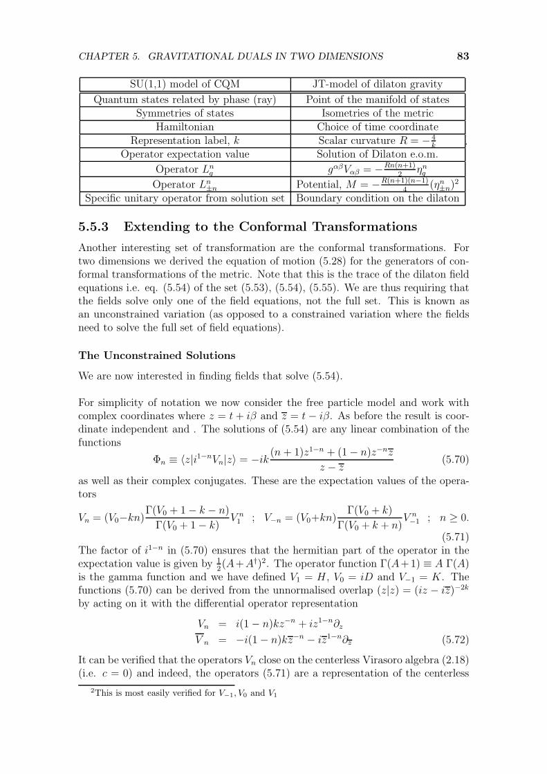
CHAPTER 5. GRAVITATIONAL DUALS IN TWO DIMENSIONS 83
SU(1,1) model of CQM JT-model of dilaton gravity
Quantum states related by phase (ray) Point of the manifold of statesSymmetries of states Isometries of the metric
Hamiltonian Choice of time coordinateRepresentation label, k Scalar curvature R = − 4
k
Operator expectation value Solution of Dilaton e.o.m.
Operator Lnq gαβVαβ = −Rn(n+1)
2ηnq
Operator Ln±n Potential, M = −R(n+1)(n−1)
4(ηn±n)
2
Specific unitary operator from solution set Boundary condition on the dilaton
.
5.5.3 Extending to the Conformal Transformations
Another interesting set of transformation are the conformal transformations. Fortwo dimensions we derived the equation of motion (5.28) for the generators of con-formal transformations of the metric. Note that this is the trace of the dilaton fieldequations i.e. eq. (5.54) of the set (5.53), (5.54), (5.55). We are thus requiring thatthe fields solve only one of the field equations, not the full set. This is known asan unconstrained variation (as opposed to a constrained variation where the fieldsneed to solve the full set of field equations).
The Unconstrained Solutions
We are now interested in finding fields that solve (5.54).
For simplicity of notation we now consider the free particle model and work withcomplex coordinates where z = t + iβ and z = t− iβ. As before the result is coor-dinate independent and . The solutions of (5.54) are any linear combination of thefunctions
Φn ≡ 〈z|i1−nVn|z〉 = −ik (n + 1)z1−n + (1− n)z−nz
z − z(5.70)
as well as their complex conjugates. These are the expectation values of the opera-tors
Vn = (V0−kn)Γ(V0 + 1− k − n)
Γ(V0 + 1− k)V n1 ; V−n = (V0+kn)
Γ(V0 + k)
Γ(V0 + k + n)V n−1 ; n ≥ 0.
(5.71)The factor of i1−n in (5.70) ensures that the hermitian part of the operator in theexpectation value is given by 1
2(A+A†)2. The operator function Γ(A+1) ≡ A Γ(A)
is the gamma function and we have defined V1 = H , V0 = iD and V−1 = K. Thefunctions (5.70) can be derived from the unnormalised overlap (z|z) = (iz − iz)−2k
by acting on it with the differential operator representation
Vn = i(1− n)kz−n + iz1−n∂z
V n = −i(1− n)kz−n − iz1−n∂z (5.72)
It can be verified that the operators Vn close on the centerless Virasoro algebra (2.18)(i.e. c = 0) and indeed, the operators (5.71) are a representation of the centerless
2This is most easily verified for V−1, V0 and V1

CHAPTER 5. GRAVITATIONAL DUALS IN TWO DIMENSIONS 84
Virasoro algebra in terms of su(1, 1) algebra elements [66].
Near the β → 0 boundary we may expand the expectation values (5.70) to find
Φn = −kt1−n
β− 1
2k(n2 − n)t−1−nβ +
i
3k(n3 − n)t−2−nβ2 +O(β3). (5.73)
The operators (5.71) are not all hermitian and we need to calculate the vector fieldswith a bit more care than previously. We write these in terms of the expectationvalues of hermitian and anti-hermitian operators (5.70). This can be done by
Φ1,n =1
2(Φn + Φ∗
n) (5.74)
Φ2,n =1
2(Φ∗
n − Φn). (5.75)
The vector fields for hermitian and anti-hermitian operators are calculated as in eq.(5.4) and we thus have
χ1,n ≡ −1
2σµν∇ν(Φ1,n)∂µ
=
(−(n− 1)t−nβ − 1
2(n3 − n)β3 +O(β4)
)∂β
+
(t1−n − 1
2(n2 − n)t−1−nβ2 +O(β4)
)∂t (5.76)
χ2,n ≡ −1
2gµν∇ν(Φ2,n)∂µ
=
(2
3(n3 − n)t−2−nβ3 +O(β4)
)∂β
+
(−1
3(n3 − n2)(n+ 2)t−3−nβ4 +O(β5)
)∂t (5.77)
The fields (5.73) and vector fields (5.76), (5.77) clearly form a power series expansion.The general form for the expectation values of the hermitian operators is any linearcombination of (5.73) and is thus given by
∑
n
an(Φn + Φ∗n) + i(Φn − Φ∗
n) =ρ(t)
β+
1
2ρ(t)β +O(β2) (5.78)
where ρ(t) =∑
n kant1−n, see eq. (5.73). Similarly the most general vector fields
are given by
∑
n
bnχ1,n = [ǫ(t)β +O(β3)]∂β + [ǫ(t)− 1
2ǫ(t)β2 +O(β3)]∂t. (5.79)
and ∑
n
cnχ2,n∂µ = [α(t)β3 +O(β4)]∂β + [1
2α(t)β4 +O(β5)]∂t (5.80)

CHAPTER 5. GRAVITATIONAL DUALS IN TWO DIMENSIONS 85
where ǫ(t) =∑
n bnt1−n and α(t) =
∑n
2cn3(n3 − n)t−2−n, see eqs. (5.76), (5.77).
The an’s, bn’s and cn’s are arbitrary expansion coefficients.
Comparing these with the transformations and field solutions of (5.43) and (5.40)reveal that the vector fields comprise the ǫ(t) and αβ(t) part of the transformations.These are precisely the transformations required to perform the analysis of section5.4.1. This is the first of two ingredients required to perform that analysis. Whatremains for us is to find the second ingredient namely the energy momentum tensoron the gravity side.
The Asymptotic (Outer Boundary) Contribution to the Central Charge
There is one thing, however, we do need to specify further. Note that between thefield solutions (5.78) and vector fields (5.79), (5.80) we have three functions of time.In the analysis of section 5.4.1 there are only two independent functions of time thatprove relevant.
This is due to the fact that, in that analysis, an additional constraint is imposed.Here we have only required that the fields satisfy (5.54) while the analysis of section5.4.1 also requires them to satisfy (5.55). At first glance this seems fundamentallydifferent to what we have done. In the analysis of section 5.4.1 the constrained fieldequations are imposed while our very starting point was that the conformal transfor-mations satisfy the unconstrained field equations3. Up to this “missing” constraintwe recover exactly the transformations used in the analysis. It thus seems that onemay recover these transformations in at least two ways - either allow the metric anddilaton to fluctuate asymptotically and impose the constrained variation or workwith an identically AdS2 metric but impose only the unconstrained variation.
What to do then about the extra function of time that we find in our analysis?The main insight is that in requiring that the fields solve the equation (5.54) we arerequiring that the trace of the energy momentum tensor is fixed. We do not placeany restriction on the potential M in the bulk. What we may specify is a boundarycondition for the potential. In [17] two possible boundary conditions are discussedand we will discuss the effects of both.
The first boundary condition is the one that will reproduce the analysis of section5.4.1 namely limβ→0∇M = 0. This means that, though we do not require (5.55) tohold in the bulk we do require it to hold near the boundary. Since the analysis iscarried out near the boundary we thus have the same allowed transformations andconstraints as in section 5.4.1.
Importantly we derived these transformations without changing the metric fromAdS2 to asymptotically AdS2. We are thus working in an AdS2 background. For
3We note that this imposing of the constrained field equations is discussed as a weakness in[67].

CHAPTER 5. GRAVITATIONAL DUALS IN TWO DIMENSIONS 86
the AdS2 metric the boundary term J is simply given by [62]
J ∝M. (5.81)
By expanding around the zero mass solution ρ = 1− ρ(t) we find
M ∝ ρ(t)2 − 2ρ(t)ρ(t) = −2ρ(t) +O(ρ2). (5.82)
The potential is thus of the appropriate form to be interpreted as an energy momen-tum tensor [67]. As mentioned in section 5.4.3 the precise normalisation still needsto be clarified. We have merely recast the arguments of section 5.4.1 in a differentset of coordinates so that we should get exactly the same contribution to the centralcharge from this calculation.
The Inner Boundary Contribution to the Central Charge
The insight that the implication of the unconstrained variation is a fluctuating po-tential term is of great value to clarify why the contribution of the inner boundaryneeds to be taken into account along with the contribution of the outer boundary.We can simply argue this in terms of the set of transformations that we allow.
The key is the boundary condition. By imposing the condition limβ→0∇M = 0we are not excluding the possibility that a transformation may be included thatchanges the potential from positive (indicative of a black hole) to zero (which isindicative of the vacuum). We know from our discussion of conformal quantummechanics (4.27) that such transformations do form part of the conformal group.Indeed, it is the transformation that maps the scale-invariant Hamiltonian to theharmonic oscillator.
This situation is clearly unacceptable since the vacuum solutions and black holesolutions are mixed. We must thus factor out the transformation that maps theblack hole solutions onto the vacuum solutions. This is the step (5.49).
We could have achieved the same feat if we started off by working with the sec-ond boundary condition proposed in [17], namely that M = fixed > 0. Indeed,in [17] they work with this boundary condition and find the correct expression forthe central charge without taking the inner and outer boundary into account. Theauthors argue that the gravitational content with these two boundary conditions aredifferent. For our purposes this is not a significant issue - we are merely interested inunderstanding how the CQM central charge may be described in the dual. Indeed,the unconstrained variation does not yield the metric as part of the field equationsolutions (5.53) and is thus not, in a strict sense, a theory of gravity. Our aim is toshow that the central charge can be incorporated in a dual description - a feat thatcan be achieved using both boundary conditions.
We conclude by again emphasising that what we have presented in this sectionare not new results in the AdS2/CFT1 context but rather show that the construc-tion we have made allow these existing results to be derived in a simple and elegant
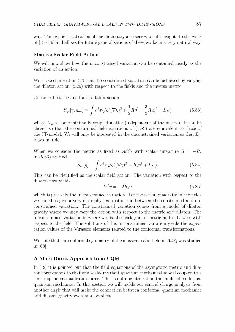
CHAPTER 5. GRAVITATIONAL DUALS IN TWO DIMENSIONS 87
way. The explicit realisation of the dictionary also serves to add insights to the workof [15]-[19] and allows for future generalisations of these works in a very natural way.
Massive Scalar Field Action
We will now show how the unconstrained variation can be contained neatly as thevariation of an action.
We showed in section 5.3 that the constrained variation can be achieved by varyingthe dilaton action (5.29) with respect to the fields and the inverse metric.
Consider first the quadratic dilaton action
Sη2 [η, gµν ] =
∫d2x
√g((∇η)2 + 1
2Rη2 − 3
2Rsη
2 + LM) (5.83)
where LM is some minimally coupled matter (independent of the metric). It can bechosen so that the constrained field equations of (5.83) are equivalent to those ofthe JT-model. We will only be interested in the unconstrained variation so that Lm
plays no role.
When we consider the metric as fixed as AdS2 with scalar curvature R = −Rs
in (5.83) we find
Sη2 [η] =
∫d2x
√g((∇η)2 −Rsη
2 + LM). (5.84)
This can be identified as the scalar field action. The variation with respect to thedilaton now yields
∇2η = −2Rsη (5.85)
which is precisely the unconstrained variation. For the action quadratic in the fieldswe can thus give a very clear physical distinction between the constrained and un-constrained variation. The constrained variation comes from a model of dilatongravity where we may vary the action with respect to the metric and dilaton. Theunconstrained variation is where we fix the background metric and only vary withrespect to the field. The solutions of this unconstrained variation yields the expec-tation values of the Virasoro elements related to the conformal transformations.
We note that the conformal symmetry of the massive scalar field in AdS2 was studiedin [68].
A More Direct Approach from CQM
In [19] it is pointed out that the field equations of the asymptotic metric and dila-ton corresponds to that of a scale-invariant quantum mechanical model coupled to atime-dependent quadratic source. This is nothing other than the model of conformalquantum mechanics. In this section we will tackle our central charge analysis fromanother angle that will make the connection between conformal quantum mechanicsand dilaton gravity even more explicit.
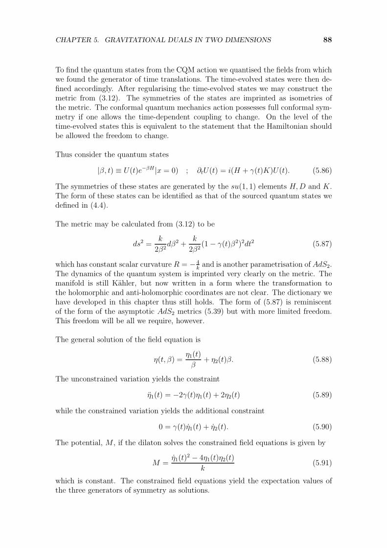
CHAPTER 5. GRAVITATIONAL DUALS IN TWO DIMENSIONS 88
To find the quantum states from the CQM action we quantised the fields from whichwe found the generator of time translations. The time-evolved states were then de-fined accordingly. After regularising the time-evolved states we may construct themetric from (3.12). The symmetries of the states are imprinted as isometries ofthe metric. The conformal quantum mechanics action possesses full conformal sym-metry if one allows the time-dependent coupling to change. On the level of thetime-evolved states this is equivalent to the statement that the Hamiltonian shouldbe allowed the freedom to change.
Thus consider the quantum states
|β, t) ≡ U(t)e−βH |x = 0) ; ∂tU(t) = i(H + γ(t)K)U(t). (5.86)
The symmetries of these states are generated by the su(1, 1) elements H,D and K.The form of these states can be identified as that of the sourced quantum states wedefined in (4.4).
The metric may be calculated from (3.12) to be
ds2 =k
2β2dβ2 +
k
2β2(1− γ(t)β2)2dt2 (5.87)
which has constant scalar curvature R = − 4kand is another parametrisation of AdS2.
The dynamics of the quantum system is imprinted very clearly on the metric. Themanifold is still Kahler, but now written in a form where the transformation tothe holomorphic and anti-holomorphic coordinates are not clear. The dictionary wehave developed in this chapter thus still holds. The form of (5.87) is reminiscentof the form of the asymptotic AdS2 metrics (5.39) but with more limited freedom.This freedom will be all we require, however.
The general solution of the field equation is
η(t, β) =η1(t)
β+ η2(t)β. (5.88)
The unconstrained variation yields the constraint
η1(t) = −2γ(t)η1(t) + 2η2(t) (5.89)
while the constrained variation yields the additional constraint
0 = γ(t)η1(t) + η2(t). (5.90)
The potential, M , if the dilaton solves the constrained field equations is given by
M =η1(t)
2 − 4η1(t)η2(t)
k(5.91)
which is constant. The constrained field equations yield the expectation values ofthe three generators of symmetry as solutions.

CHAPTER 5. GRAVITATIONAL DUALS IN TWO DIMENSIONS 89
The potential, when only the unconstrained field equation (5.89) is imposed, isgiven by (in an expansion around β = 0)
M =η1(t)
2 − 4η1(t)η2(t)
k+
2(γ(t)η1(t) + η2(t))η1(t)β2
k+O(β3). (5.92)
In (5.92) the difference between the constrained and unconstrained variation is clear.The constrained variation yields a constant value for M while the unconstrainedvariation allows for asymptotic correction terms. In [19] the authors identify theasymptotic corrections with the kinetic energy of the conformal quantum mechan-ical model. We showed in section (4.5), our discussion of conformal quantum me-chanics, that the time-dependent coupling (after conformal transformation) is dueto the kinetic term.
The transformation properties of the dilaton gravity potential M can thus clearlybe used to extract the central charge. The interpretation of a changing couplingterm, γ(t) in CQM is thus that the potential of dilaton gravity, related to the blackhole mass, is allowed to fluctuate asymptotically.
We thus present the following additions to the dictionary for conformal quantummechanics and dilaton gravity
Conformal Quantum Mechanics JT-model of dilaton gravity
Local Symmetries Conformal transformations of the metricExpectation values of Dilaton solutionsconformal generators in unconstraind variation
Changing γ(t) Asymptotic fluctuations in M
5.5.4 The Duals of the SU(2) Quantum Models
We next examine the SU(2) Hamiltonian systems. As we showed (4.57) we findthat the scalar curvature is also constant as it was for the SU(1, 1) models. Theonly adjustment we need to make is the sign of the scalar curvature so that we nowconsider a dS2 background as opposed to an AdS2 background. Two dimensionalde Sitter geometries have been considered in the context of dualities before, mostnotably in the dS2/CFT1 correspondence [69], [70]. The field equation (5.28) holdsfor the conformal transformations of any two-dimensional metric so that the confor-mal transformations of dS2 can be handled on similar footing to AdS2.
The su(2) and su(1, 1) algebras are related by an appropriate complexification ofthe generators. It should thus be possible to perform an analysis that is very similarto the AdS2/CFT1 analysis we carried out in the previous section (which may becompared to [69], [70]). This will not be done here and is a possible avenue forfuture study.
Our interest here is simply to recover the expectation values of operators from the

CHAPTER 5. GRAVITATIONAL DUALS IN TWO DIMENSIONS 90
SU(2) enveloping algebra by means of a dual description and we will show now thatthis can be done. The SU(2) coherent states are given in (4.55). The dilaton model
SSU(2) =
∫dzdz
√g(R − 2
j)η (5.93)
yields, up to a coordinate transformation, the metric (4.57) as the on-shell solution.The dilatons that solve the on-shell field equation are the expectation values of thesymmetry generators
〈z|Jz|z〉 = j(zz − 1)
zz + 1,
〈z|12(J+ + J−)|z〉 = j
z + z
1 + zz,
〈z| i2(J+ − J−)|z〉 = ij
z − z
1 + zz, (5.94)
with respect to the SU(2) coherent states. The trace of the energy momentumtensor is gαβVαβ = −R = −2
j. Again these expectation values are related to the
Killing vectors (4.58) by the symplectic structure (5.4). The potential associatedwith the operators uJz +
v2(J+ + J−) +
iw2(J+ − J−) is
M =j
2(u2 + v2 + w2). (5.95)
This is constant, as it should be for a generator of symmetry. Furthermore, it isalways positive, unlike for the SU(1, 1) duals, so that we do not get geometries thatare different globally. As before operators that share the same mass are related bya unitary transformation.
It is worthwhile to reflect on the difference between this case and that found in[69] where three globally different solutions are in fact found. We suspect that thisis due to considering the representation of SU(2) related to the infinite dimensionalSU(1, 1) representation by a complexification of operators. The consequence of thisis that additional factors of i are introduced. If we allow the coefficient u, v and wto assume complex values then the sign of M can be altered. The dilaton solutionsare then rather the expectation values of non-hermitian operators. The precise linkbetween these two analyses warrant further investigation.
For our current purposes we only wish to calculate the expectation values of su(2)algebra elements and for this the use of (5.95) is sufficient. One can proceed tofind the appropriate energy momentum tensors for the enveloping algebra from thispoint in similar fashion to before. The Laplacian is, as before, a representation ofthe Casimir and we may classify the expectation values of su(2) eveloping algebraoperators in terms of their eigenvalues with respect to the differential operator rep-resentation of the Casimir and Jz. The procedure is analogous to that performed insection 5.5.2. One finds that
∇2〈z|(J+)n|z〉 = −Rn(n + 1)
2〈z|(J+)n|z〉 (5.96)
M(J+)n = −R(n + 1)(n− 1)
4(〈z|(J+)n|z〉)2 (5.97)

CHAPTER 5. GRAVITATIONAL DUALS IN TWO DIMENSIONS 91
This allows one to calculate the expectation value of any element of the evelopingalgebra of su(2) in the dual dilaton gravity description. As before this is done byincluding the appropriate energy momentum tensor.
5.6 The dual of the Glauber Coherent States
The metric constructed from the Glauber coherent states (4.60) is flat. This presentsa very unique situation since the trick we employed to get rid of the constant c in(5.22) is no longer applicable. Indeed, it can be verified that the expectation values
〈z|c1a† + c2a|z〉 = c1z + c2z (5.98)
satisfy the equations of the previous sections ∇µ∇νη = 0 with R = 0 and thatthe mass is given by the product c1c2. However, the expectation value of the thirdgenerator of symmetry
〈z|a†a|z〉 = zz (5.99)
rather satisfies the equation∇µ∇νη = gµν (5.100)
so that c = 1 in (5.22). The mass associated with this equation and solution is zero.It is thus not possible to capture all the generators of symmetry into a single actionand distinguish them up to the choice of mass. For the operators (5.98) the action
S =
∫dzdz
√gRη (5.101)
works but for the number operator expectation value (5.99) we need a differentaction of the form
S =
∫dzdz
√g(Rη + 2η). (5.102)
Due to the fact that we cannot eliminate the constant λ in (5.22) we cannot findan action of which the field equations are solved by the expectation values of thealgebra elements simultaneously. The expectation values of the algebra elements isthus better served by considering it as a large j limit of the su(2) algebra elements.
This indicates that for a neat and sensible dictionary a non-zero curvature of themanifold is essential.
5.7 Summary
In this chapter we investigated 2d gravity duals. We managed to develop a sys-tematic dictionary between quantum mechanical models and a JT-model of dilatongravity. We investigated the details of this dictionary for the Glauber coherentstates, the SU(2) Hamiltonians and, in particular, the SU(1, 1) quantum models.We were able to show how numerous existing results in the AdS2/CFT1 literaturecome about in a very natural way from our construction. We were also able to

CHAPTER 5. GRAVITATIONAL DUALS IN TWO DIMENSIONS 92
expand upon some of their results and identified several avenues of possible futureinvestigation.
These results comprise the core results of this thesis. They should not be viewedas a calculational procedure but rather a proof of concept. It shows that quantummechanical systems can be repackaged as gravity duals, at least in two dimensions,and that this can be done systematically. The number of existing results from theAdS2/CFT1 literature that are reproduced in a natural way from our construc-tion seems to indicate that the construction repackages these quantum mechanicalsystems in an appropriate way. Furthermore, the systematic construction gives usdirect and full access to the quantum mechanics / dilaton gravity dictionary. Thisprovides a significant level of clarity to the AdS2/CFT1 correspondence.
In the remaining chapters we will investigate the higher dimensional manifolds,the difficulties that arise when one wishes to build gravitational duals and proposedsolutions to these difficulties. We will again see existing results from the literaturecome about in a very natural way but our investigations will not be as well-developedas they have been in this chapter.
Chapter 6
A Look at Higher DimensionalModels
Our focus thus far has been on the two-dimensional manifolds of states. The reasonfor this is clear - it is the simplest example of our construction. Our focus has, inparticular, been on time-evolved states where the time-coordinate is complexified.Existing results of the AdS2/CFT1 correspondence were shown to follow from theconstruction in a natural way and we were also able to extend these results. Wefurther showed that more general dual gravitational models, that do not have anAdS2 geometry, can be constructed in a systematic way, starting from an appropri-ate choice of quantum states.
We will now turn to higher dimensional models. The most natural extension tohigher dimensions is to include a position label for the states. As before, in orderto utilise results the geometric formulation of quantum mechanics of Ashtekar andSchilling, discussed in section 3.3, we will consider states labelled by complex coor-dinates. This will present a difficulty since, unlike in two dimensions, the Kahlermanifolds in higher dimensions are not maximally symmetric. This will lead to ad-ditional terms in the equations of motion for the expectation values of operators.
Our study will thus almost immediately specialise to the simplest higher dimen-sional models, those that have full Schrodinger group symmetry (such as the freeparticle and harmonic oscillator). Though this is a significant simplification it servesas a starting point to understanding the higher dimensional duals.
We will motivate, after analysis of these models, why a central extension of theSchrodinger algebra is a beneficial procedure. In chapter 7 we will analyse the met-rics that are produced from states where this central extension is considered as adynamic quantity.
6.1 The Equations of Motion
We assume that the family of states are parametrised by n complex parameters i.e.|z1, ..., zn). Note that the dimension of the state manifolds is 2n. We have already
93

CHAPTER 6. A LOOK AT HIGHER DIMENSIONAL MODELS 94
derived the equations of motion for the expectation value, Φ of an arbitrary operatorin section 5.2, but restate it here for convenience
σ ǫγ ∇α∇β∇ǫΦ = R δ
γβα σǫ
δ ∇ǫΦ− 1
2ταβγ . (6.1)
In two dimensions we were able to use the simple form for the Riemann curvaturetensor (5.18) to derive, from (6.1), simple equations of motion with at most sec-ond order derivatives. In the higher dimensional case the Riemann tensor is morecomplicated (see Appendix A) which adds additional terms to the equations. For2n > 2, we have that [71]
Rαβγδ = Wαβγδ
+1
2n− 2(Rαγgβδ +Rβδgαγ −Rαδgβγ − Rβγgαδ)
− R
(2n− 1)(2n− 2)(gαγgβδ − gαδgβγ) (6.2)
where Wαβγδ is the Weyl tensor. The Weyl tensor encodes information on the con-formal properties of the metric in that the Weyl tensor is zero if and only if themetric is conformally flat [71]. This more complicated form for the Riemann tensormakes the higher-dimensional analysis more intricate. In this thesis we will try tosimplify the equations as much as possible.
As a first simplification we note that the contraction of the Weyl tensor underany two indices is zero so that we first consider only the trace of the field equations(6.1). We then arrive at
σ ǫγ g
αβ∇α∇β∇ǫΦ ⇒ ∇ǫ∇2Φ = −σ γǫ R
δγ σ
αδ ∇αΦ− R δ
ǫ ∇δΦ. (6.3)
Note that if we are working with an Einstein manifold i.e. Rµν = R2ngµν this simplifies
to
∇ǫ∇2Φ = −Rn∇ǫΦ (6.4)
and, if in addition the scalar curvature is constant, we find
∇2Φ = −RnΦ. (6.5)
The trace of the field equations, at least for an Einstein metric of constant scalarcurvature, is of the simple form (6.5). We will see in section 6.2 that even for thefree particle states the resulting metric is not Einstein. Indeed, we will only producemetrics that are Einstein (in more than two dimensions) in chapter 7.
If the metric is not Einstein then the trace of the field equations are more com-plicated. We express the Ricci tensor as Rµν = R
2ngµν + Rµν where gαβRαβ = 0 and
take the trace of (6.3) to find
∇ǫ∇2Φ = −Rn∇ǫΦ− σ γ
ǫ Rδ
γ σα
δ ∇αΦ− R δǫ ∇δΦ
= −∇ǫ
(R
nΦ
)+
(Φ
n∇ǫR − σ γ
ǫ Rδ
γ σα
δ ∇αΦ− R δǫ ∇δΦ
). (6.6)
CHAPTER 6. A LOOK AT HIGHER DIMENSIONAL MODELS 95
If the second term of (6.6) is zero then we recover (6.5). If not then our equations ofmotion will look quite different. If, in addition we are not sourcing the expectationvalue of a symmetry generator then this will add an additional term in (6.6). Notethat the second term has contributions from a scalar curvature that is not constantand a Ricci tensor that is not Einstein. The best situation we can hope for is thatwe can contain the deviation from (6.5) in a single scalar function
∇2Φ = −RnΦ+ V (Φ) (6.7)
where V gets contributions if the scalar curvature is not constant, the manifold isnot Einstein and the expectation value being sourced is not a generator of symmetry.
The trace of the field equations (6.3) thus only assumes the form of an eigenvalueproblem for the expectation values of symmetry generators (6.5) if both the scalarcurvature is constant and the metric is Einstein. If we were to consider the full setof field equations (6.3) we would have to account for a non-zero Weyl tensor as well.In this thesis we will not study the latter so that the analysis of the full set of fieldequations is a possible avenue of future investigation. Note, importantly, that sincewe are only considering the one field equation we will need to specify additionalboundary conditions in order to source the appropriate expectation value. We willspeak to this more in section 7.3.
6.1.1 Massive Scalar Field
Before we proceed to look at a specific higher dimensional example we will show howthe field equation (6.5) may result from the variation of an action. We have alreadyintroduced this action in section 5.5.3 but we restate it here for higher dimensions
S =
∫ddx
√g((∇Φ)2 +m2Φ2 + 2V (Φ)
). (6.8)
The action (6.8) is defined on a fixed background. The field equation is found byvarying with respect to the field Φ
δS
δΦ= 0 ⇒ ∇2Φ = m2Φ + ∂ΦV (6.9)
which is exactly of the form (6.7) if m2 = −2Rd
and ∂ΦV = V (Φ).
Along with the field equation we will have to specify boundary conditions. Thisis best illustrated by example e.g. in section 7.3.
6.2 The Schrd+1 Models
The Schrodinger algebra for two dimensions (time and one spatial dimension) is givenin (3.6) and the extension to higher dimensions is straightforward (see Appendix C).
CHAPTER 6. A LOOK AT HIGHER DIMENSIONAL MODELS 96
Instead of a single position operator X and momentum operator P we have d i.e.X1, X2, ..., Xd and P1, P2, ..., Pd related by rotation. These then satisfy
[Xi, Pj] = iδij . (6.10)
For the sake of illustration we restrict ourselves to a concrete example namely thefree particle states
eitHei~x·~P |x = 0) → ei(t+iβ)Hei(~x+i~y)·~P |x = 0) ≡ eiτHei~z·
~P |x = 0) (6.11)
though, as discussed in the context of the 2d metrics, any Hamiltonian from theschrd+1 algebra, such as the harmonic oscillator, will yield states that are related by acoordinate transformation and normalisation to the states (6.11). Note the definitionof the coordinates t, β, xj and yj in (6.11). We will work with β, t, x1, y1, ..., xd, ydcoordinates and τ, τ , z1, z1, ..., zd, zd coordinates interchangeably. Note that wehave n = d+ 1 complex coordinates. The overlap of these states (6.11) is given by
(τ, ~z|τ, ~z) = (iτ − iτ)−d2 e−i
(~z−~z)2
2(τ−τ) (6.12)
which is simply the complexified and unnormalised free particle propagator. Theinteger d refers to the number of spatial dimensions. From the overlap (6.12) themetric may be calculated to be
ds2 =dβ + 4~y · ~y
8β3
(dβ2 + dt2
)− 1
β2(~y · d~ydβ + ~y · d~xdt) + 1
2β
(dy2 + dx2
). (6.13)
The scalar curvature is constant, R = −8(d+2)d
but the manifold is not Einstein.Specifically there are only two non-zero entries for the Ricci tensor
Rττ = Rττ = −d+ 2
2β2. (6.14)
The equations of motion for the expectation values of symmetry generators arethus not of the form (6.5) so that these expectation values cannot be found aseigenfunctions of the Laplacian.
6.2.1 Examining the Laplacian
In section 5.5.2 we were able to derive the trace of the energy momentum tensor byobserving that the Laplacian is a differential operator representation of the su(1, 1)Casimir. This was because the Killing vectors formed a vector field representation ofthe su(1, 1) algebra elements and all the Killing vectors commute with the Laplacian.
The situation for the schrd+1 algebra is slightly different. A dynamical symme-try (3.1) only implies a non-zero Killing vector if it is not simply a change of phasefor the family of states. The commutator of Xi and Pi (6.10) will simply change thephase of the wave function. While the operators X and P thus satisfy (6.10) theircorresponding vector fields satisfy
[χPi, χXj
] = 0 ∀ i, j. (6.15)

CHAPTER 6. A LOOK AT HIGHER DIMENSIONAL MODELS 97
This implies that the Killing vectors no longer close on the Schrodinger algebra. Asan example, the Laplacian in four dimensions is given by
∇2 = 8β2(∂2β + ∂2t ) + 16βy(∂β∂y + ∂t∂x) + 2(β + 4y2)(∂2y + ∂2x) (6.16)
and commutes with all the Killing vectors, χH , χD, χK , χPi, χXj
but is not theSchrodinger algebra Casimir (see e.g. [72]) in differential operator form. The proce-dure of section 5.5.2, where we classified the expectation values of operators of theenveloping algebra by their eigenvalues with the Casimir and scaling operator, willthus not work here.
One of the natural questions to ask is whether the eigenfunctions of the Laplaciancan still be interpreted as the expectation values of operators from the envelopingalgebra of schrd+1. To begin answering this question we first state the expectationvalues of the generators of symmetry explicitly
〈τ, ~z|H|τ, ~z〉 =d
4β+
~y2
2β2,
〈τ, ~z|D|τ, ~z〉 =dt
4β+~y · (t~y − β~x)
2β2,
〈τ, ~z|K|τ, ~z〉 =d(t2 + β2)
4β+
(t~y − β~x) · (t~y − β~x)
2β2,
〈τ, ~z|Pj |τ, ~z〉 =yjβ,
〈τ, ~z|Xj |τ, ~z〉 =tyj − βxj
β. (6.17)
Note that the SU(1, 1) generators are all of the form
〈τ, ~z|A|τ, ~z〉 = 〈τ,~0|A|τ,~0〉+ 1
2
d∑
i=1
〈τ, ~z|B1,i|τ, ~z〉〈τ, ~z|B2,i|τ, ~z〉 (6.18)
where B1,i = B2,i = Pi, B1,i = B2,i = Ki and B1,i = Pi, B2,i = Ki for H,K andD respectively. On the ~z = ~z = ~0 submanifold the expectation values, metric andRicci tensor thus look identical to the two-dimensional su(1, 1) case. This may beunderstood intuitively since the underlying algebra, the Schrodinger algebra, is thesemi-direct sum of su(1, 1) and d Heisenberg algebras (related by rotation) i.e. somecombination of an AdS2 and d flat space geometries. The ~z = ~z = ~0 submanifold isprecisely the AdS2 submanifold.
Based on this one might venture a guess that a subset of the eigenfunctions ofthe Laplacian are the expectation values of operators restricted to the AdS2 sub-manifold. This turns out to be the case and, for the operators Lq
n (defined in section5.5.2) we find the relation
∇2〈τ,~0|Lqn|τ,~0〉 = − R
d+ 2n(n + 1)〈τ,~0|Lq
n|τ, 0〉 (6.19)

CHAPTER 6. A LOOK AT HIGHER DIMENSIONAL MODELS 98
where |τ, 0〉 = eiτH |~z = 0). In addition to this the expectation value of the positionand momentum operators are eigenfunctions of the Laplacian
∇2〈τ, ~z|Pj|τ, ~z〉 = 0 = ∇2〈τ, ~z|Xj|τ, ~z〉 (6.20)
6.2.2 Eigenfunctions of the Laplacian
Of course, the expressions (6.19) are not expectation values with respect to the|τ, ~z〉 basis. Using the relations (6.17), (6.18) and (6.19) we may deduce that theexpectation value
〈τ, ~z|δAiδBi|τ, ~z〉 = 〈τ, ~z|AiBi|τ, ~z〉 − 〈τ, ~z|Ai|τ, ~z〉〈τ, ~z|Bi|τ, ~z〉 (6.21)
where Ai, Bi ∈ Xi, Pi is an eigenfunction of the Laplacian. This can be written ina much more suggestive form following eq. (5.13)
〈τ, ~z|δAiδBi|τ, ~z〉 =1
2〈τ, ~z|δAi, Bi|τ, ~z〉 =
1
2χµiAi∂µ〈τ, ~z|Bi|τ, ~z〉 (6.22)
which suggest that the vector fields χiO may be used in some ladder operator schemeto find the eigenfunctions of the Laplacian. Indeed, this turns out to be case.
The eigenfunctions of the Laplacian (6.16), f qj,n may be labelled by three indices
n ∈ N, q ≤ |n| and j ∈ 0, 1, ..., d. The explicit meaning of these indices willbecome clear shortly. The starting point of the laddering scheme is one of the dexpectation values of momentum. One can then ladder up in n by means of χiH
immediately or first apply χiP and then ladder up in n by means of χiH i.e.
f−nj,n = (χµ
iH∂µ)n−1 〈τ, ~z|Pj |τ, ~z〉,
f−n0,n = (χµ
iH∂µ)n−1(χνiPj∂ν
)〈τ, ~z|Pj|τ, ~z〉. (6.23)
At this point the explicit forms of these functions may be useful for the sake offollowing the argument
f−nj,n ∝ yj
βn; f−n
0,n ∝ 1
βn; χµ
iH∂µ = ∂β ; χνiPj∂ν = ∂yj . (6.24)
The expressions (6.24) may be used to verify the statements we make. We prefer towrite the expressions with (6.23) since these expressions do not make use of a choiceof coordinates. The eigenfunctions (6.23) are the lowest tiers in terms of ladderingin the index q since χν
H∂νf−nj,n = 0. We may ladder up in the index q by means of
χK i.e.f q+1
j,n = χµK∂µf
qj,n (6.25)
so that the index q is related to the eigenvalue with respect to χD. The index nis related to the eigenvalue with respect to the Laplacian. Explicitly, most easilyverified for the functions (6.23), one has
χνD∂νf
qj,n = (q +
1
2)f q
j,n ; ∇2f qj,n = − R
d+ 2n(n− 1)f q
j,n (6.26)
χνD∂νf
q0,n = qf q
0,n ; ∇2f q0,n = − R
d+ 2n(n+ 1)f q
0,n. (6.27)

CHAPTER 6. A LOOK AT HIGHER DIMENSIONAL MODELS 99
The index j thus divides the eigenfunctions into two classes, those with eigenvalues(6.26) if j is non-zero and (6.27) if j = 0. Note that the functions with non-zero jare related simply by rotation.
6.2.3 Eigenfunctions Expressed as Operator ExpectationValues
The expressions (6.23) and (6.25) now express the eigenfunctions of the Laplacianas some combination of expectation values of operators with respect to the states|τ, ~z〉. A few examples of these are
f 0j,0 = 〈τ, ~z|Pj|τ, ~z〉,
f−1j,1 = 〈τ, ~z|HPj|τ, ~z〉 − 〈τ, ~z|H|τ, ~z〉〈τ, ~z|Pj|τ, ~z〉,
f−2j,2 = 〈τ, ~z|δHHPj|τ, ~z〉 − 〈τ, ~z|δHH|τ, ~z〉〈τ, ~z|Pj|τ, ~z〉
−〈τ, ~z|H|τ, ~z〉〈τ, ~z|δHPj|τ, ~z〉. (6.28)
Though the eigenfunctions of the Laplacian are not interpretable directly as theexpectation values of operators (instead they are combinations of products of ex-pectation values), they may be used to calculate a specific expectation value of anoperators.
6.2.4 The Structure of the Laplacian in Terms of the
schrd+1 Algebra
We suspect that these results may be better understood if the Laplacian can berecast in terms of the schrd+1 operators. Unfortunately, our studies thus far havenot revealed how this may be done and this is an avenue of future investigations.
What we find intriguing is the fact that the eigenfunctions form two classes - thosethat are generated by a series of ladder operators on 〈P 〉 and on 〈δPδP 〉 (6.23). Theeigenvalues for these two classes are different, but the difference between eigenvaluesis the same.
This is reminiscent of selecting the even or odd sector in the su(1, 1) representa-tion i.e. the k = 1
4or k = 3
4representation. More explicitly, the su(1, 1) operators
(4.16) may be represented in terms of creation and annihilation operators
K0 =1
2a†a+
1
4; K+ =
1
2a†a† ; K− =
1
2aa (6.29)
where [a, a†] = 1. The coherent states for su(1, 1) will be of the form ezK+|φ0) for twochoices of |φ0) namely the eigenstates |0〉, |1〉 of a†a i.e. K0|0〉 = 1
4and K0|1〉 = 3
4.
The coherent states will then be a combination of the even states |2n〉 or the oddstates |2n+ 1〉. The operators that relate the even and odd sectors are a and a†.
The states we are considering (6.11) are the result of the Schrodiger group act-ing on the reference state |0〉. The Schrodinger group, in turn, can be viewed as the

CHAPTER 6. A LOOK AT HIGHER DIMENSIONAL MODELS 100
semi-direct sum of SU(1, 1) and d Heisenberg groups (see appendix D) related byrotation. In a certain sense we are thus mixing the k = 1
4and k = 3
4representations.
If we only restrict ourselves to (a specific combination of) the operators with evenpowers of P and X we get the expressions (6.27) while odd powers yield (6.26).These are the expressions we would expect if we simply calculated the eigenvaluesfor the su(1, 1) enveloping algebra elements in the two different representations, seesection 5.5.2.
These statements can only be made rigorous once the Laplacian is recast in termsof schrd+1 algebra elements. We hope to do this in future.
6.3 Notable Submanifolds
In chapter 7 we will seek to put together a dual description that is simpler thanthat of section 6.2. One may anticipate what we will do when it is observed thatthe Laplacian is not a differential operator representation of the Schrodinger algebraCasimir.
The reason the Laplacian is not a representation of the Schrodinger algebra Casimiris because the Killing vectors do not close on the schrd+1 algebra which in turn isthe consequence of the commutator between Xj and Pj only changing the phase ofthe states. In order for it to be represented as a non-zero Killing vector we will haveto ensure that it represents a non-trivial transformation of the states.
Before we continue to do this we briefly highlight some of the interesting mani-folds that result if not all of the coordinates of the states (6.11) are complexified.We will introduce only a single complex coordinate. Of course, this will spoil the re-lation between the Killing vectors and the expectation values of operators. In orderto develop a dictionary for these manifolds a lot more work will be required, a dis-cussion undertaken in section 7.5. Nonetheless, these metrics are interesting becausethey are studied in the literature and illustrate some properties of the constructionwe have not yet encountered.
6.3.1 Complexified Time
Consider the regularisation scheme where we only complexify time i.e. t → t + iβin (6.11). This breaks all symmetries generated by Xi and K in the bulk (β > 0)and produces the metric
ds2 =k
2β2
(dβ2 + dt2
)+k
βd~x2. (6.30)
After the transformation β = 1r2
this becomes
ds2 = k
(4dr2
r2+r4
2dt2 + r2d~x2
)(6.31)
CHAPTER 6. A LOOK AT HIGHER DIMENSIONAL MODELS 101
which is the metric studied in [73] when considering Lifshitz-like fixed points. ALifshitz-like fixed point is a scale invariant fixed point where space and time scaleas x → λx and t → λzt. In [73] the authors focus on the case z = 2. This scaleinvariance is reflected in the metric as an isometry. Note that the states on theboundary β → 0 are still the states (6.11). This illustrates that the bulk for a dualtheory is not unique and, in particular, depends on the regularisation scheme chosen.
6.3.2 Momentum Regularisation
We may regularise the states in another way, by means of the absolute value ofmomentum. We consider the states
|r, t, ~x) = eitHei~x·~Pe−r|~P ||~x = ~0). (6.32)
There are other schemes that use functions of powers of |Pj| but the scheme (6.32)is chosen so that rotational symmetry remains unbroken. However, as with (6.30)the symmetries generated by Xi and K are broken. For d = 1, for example, thisyields the metric
ds2 =1
4r2dr2 − 1
2r3dtdr +
5
16r4dt2 +
1
2r2dx2, (6.33)
which is clearly a different metric to (6.30). Even though the symmetries we retainin the bulk are the same and the states on the boundary of the manifold of statesare identical the bulk geometry is different. This illustrates that the regularisationscheme we choose has a significant effect on the geometry.
Note that the interpretation of the radial coordinate is also different. In (6.30)it has the interpretation of an energy scale while in (6.33) it has the dimension oflength. There is thus not a general interpretation of the radial coordinate.
6.4 Discussion
In this chapter we sought to extend the two-dimensional gravitational duals of chap-ter 5 to higher dimensions. As one may expect the equations of motion becomesignificantly more complicated in higher dimension. The Riemann curvature hascontributions from the scalar curvature, the Ricci tensor and the Weyl tensor. Thesecannot be avoided altogether since no Kahler manifold in four dimensions or higheris maximally symmetric.
In order to simplify matters we focused solely on the trace of the field equations.The Weyl tensor is zero under any contraction of indices so that the trace of theequations of motion are not affected by the Weyl tensor. The trace of the equationsyield a Laplacian. We took note of the fact that, if the manifold is Einstein withconstant scalar curvature, the expectation values of symmetry generators are eigen-functions of the Laplacian.

CHAPTER 6. A LOOK AT HIGHER DIMENSIONAL MODELS 102
We then proceeded to analyse a specific example - states with Schrodinger sym-metry which is the natural extension of the su(1, 1) states to higher dimensions.The resulting manifold is, however, not Einstein and the Laplacian is not a repre-sentation of the Schrodinger algebra Casimir. We managed to develop a scheme bywhich the expectation values of operators may be extracted from the eigenfunctionsbut further work is needed to understand this structure properly.
In the next chapter we will seek to restore the status of the Laplacian as a rep-resentation of the Casimir. This will allow us to interpret its eigenfunctions as theexpectation values of operators so that the dictionary of chapter 5 may be extendedto higher dimensions more simply.
Chapter 7
Free Particle Metrics withDynamical Mass
In this chapter we will proceed to centrally extend the Schrodinger algebra in or-der to construct dual gravitational theories that are as simple as possible for theSchrodinger Hamiltonian models. Specifically we hope that this will restore theLaplacian to a differential operator representation of the Casimir. The dictionarywe will be able to develop should then be closely related to that of chapter 5.
We note that metrics containing the Schrodinger symmetry have received inter-est before. In [20], [21] the authors aim to generalize the AdS/CFT correspondenceto the case of non-relativistic field theories, or AdS/NRCFT . As is the usual casefor dual descriptions the symmetries play a crucial role. The symmetry generatorsthey consider, that of NRCFT , close on the conformal Galilei algebra [20] of whichthe Schrodinger algebra of chapter 6 is an example. The conformal Galilei groupwill thus be our starting point in this chapter.
This chapter can be divided into three parts. In the first we will show how consider-ing the mass (the central extension of the conformal Galilei group) as a dynamicalvariable will allow for the definition of a set of quantum states that have a simplegravitational dual. Specifically we will find that the expectation values of symmetrygenerators may be sourced by a traceless energy momentum tensor, precisely thedesired result. We will conclude this part with a dictionary applicable to the com-plex free particle states in higher dimensions.
In the second we will show how metrics studied in the AdS/NRCFT correspon-dence literature [20], [21] may be derived using our construction. This can be doneby either an appropriate choice of quantum states or viewing the metrics as definedon submanifolds of a Kahler manifold. This will supplement their works by identi-fying the explicit quantum states that constitute the quantum theory of the duality.These observations, along with the systematic nature of the construction, holds thepromise of future generalisations to these studies.
These submanifolds will in general not be Kahler themselves and thus the dual-
103

CHAPTER 7. FREE PARTICLE METRICS WITH DYNAMICAL MASS 104
ity between the expectation values of operators and Killing vectors breaks down.In the last section we will speculate as to how a dictionary for the submanifoldsmay be developed. We would like to warn the reader beforehand that the discussioncontained therein will be qualitative at best. Therein we wish only to convey someof our ideas on how one may progress beyond the work done in this thesis.
7.1 The Conformal Galilei Algebra
We start by defining the d+1 dimensional conformal Galilei algebra (see AppendixC) which consists of 1
2d(d − 1) rotations, d + 1 translations, d Galilean boosts,
dilatations and the rest mass. These are generated by Mij, Pi+H , Gi, D and Nwhich satisfy the (non-zero) commutation relations
[Mij ,Mkl] = i(g0ikMjl + g0jlMik − g0ilMjk − g0jkMil)
[Gi,Mkl] = i(g0ikXl − g0ilKk) ; [Pi,Mkl] = i(g0ikPl − g0ilPk)
[Gi, Pj] = iδijN ; [D,Pi] = − i
2Pi
[D,Gi] =i
2(z − 1)Gi ; [D,N ] =
i
2(z − 2)N
[H,Gi] = −iPi ; [D,H ] = −z2iH (7.1)
where z is the so-called dynamical exponent and the (Latin) indices run from 1 → d.The operator N represents the central extension of the algebra and we will refer toit as the mass operator or mass for short. This is the d + 1-dimensional conformalGalilei algebra with dynamical exponent z, cgal 2
z(d + 1) [74]. The dynamical ex-
ponent characterises the different scaling behavior of time and spatial coordinates.The tensor g0µν is the flat space metric and we immediately specialise to Euclideansignature i.e. g0µν = δµν . When z = 2 there is also a special conformal generator Kwhich satisfies
[K,Pi] = iGi ; [D,K] = iK ; [H,K] = 2iD (7.2)
and the algebra is the d+1 dimensional Schrodinger algebra schr(d+1) [75]. In thischapter we will show how metrics that encode the cgal 2
z(d + 1) transformations as
isometries may be constructed from appropriately chosen quantum states via (3.12).We will also provide a second perspective namely that they may be viewed as themetric of a submanifold of the Kahler manifold.
7.1.1 Representation in Terms of Quantum Mechanical
Operators
The operator N is the central extension of the algebra which is a first step torestoring the status of the Laplacian as the Casimir. The central extension by itselfis not sufficient, however. This is because the central extension still commutes withall elements of the Schrodinger algebra (see (7.1)) so that the transformation itinduces on the quantum states is still only a phase shift. In order for it to induce

CHAPTER 7. FREE PARTICLE METRICS WITH DYNAMICAL MASS 105
a non-trivial transformation we will consider the mass, N , as a dynamical variableand introduce a new operator Z such that
[Z,N ] = i. (7.3)
We will refer to Z as the conjugate mass. The inclusion of Z also allows us to rep-resent the elements of algebra (7.1) in terms of Z, N and position and momentumoperators (we were able to do this previously for z = 2 but not for general z).
The momentum operators are simply the Pi’s and the position operators can berecovered as Xi = N−1Gi. The operators H , Mij and K can be represented interms of momentum, Pi, and position, Xi, operators as
12N
∑i P
2i ,
1N(PiXj − PjXi)
and 12N
∑iG
2i respectively. Note that these representations are independent of the
dynamical exponent and thus hold for any one of the cgal 2z(d + 1) algebras. The
dilatation operator D on the other hand does depend on the dynamical exponentand may be represented as D = − 1
4N
∑i (XiPi + PiXi)+
(z−2)4
(ZN +NZ). Clearlywe recover the representations in terms of position and momentum (3.5) for theSchrodinger algebra when z = 2.
The sets of operators Z,N and Xi, Pi are such that operators from differentsets commute with each other and may thus be combined in a tensor product struc-ture in a simple way. This will be done shortly.
7.2 The Dynamical Mass Tensor Product States
We will now construct the quantum states that incorporate the dynamical mass. Theaim here is for the operatorN to induce a non-trivial transformation on the quantumstates so that its action induces a coordinate transformation on the resulting metric.
We note that this procedure of considering the mass as a dynamical variable corre-sponds to the prescription of Giulini [76] to introduce the Bargmann superselectionrule in quantum mechanics. Good discussions on the requirement for and the roleplayed by the superselection rule can be found in [76], [77], [78]. Note, however,that the states we have worked with in the previous chapters are mathematicallyconsistent and physically relevant and one may consider quantum mechanics withor without the superselection rule imposed.
We will, in order to keep close contact with the physics, work with the representa-tion of the operators in terms of Xi, Pi, N, Z. See Appendix E for the examinationof the relevant algebras in terms of abstract elements. The commutation relations,
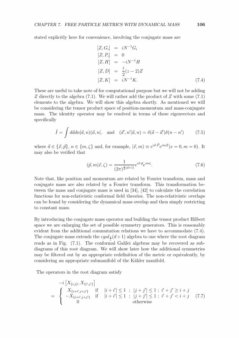
CHAPTER 7. FREE PARTICLE METRICS WITH DYNAMICAL MASS 106
stated explicitly here for convenience, involving the conjugate mass are
[Z,Gi] = iN−1Gi
[Z, Pi] = 0
[Z,H ] = −iN−1H
[Z,D] =i
2(z − 2)Z
[Z,K] = iN−1K. (7.4)
These are useful to take note of for computational purpose but we will not be addingZ directly to the algebra (7.1). We will rather add the product of Z with some (7.1)elements to the algebra. We will show this algebra shortly. As mentioned we willbe considering the tensor product space of position-momentum and mass-conjugatemass. The identity operator may be resolved in terms of these eigenvectors andspecifically
I =
∫d~adn|~a, n)(~a, n|. and (~a′, n′|~a, n) = δ(~a− ~a′)δ(n− n′) (7.5)
where ~a ∈ ~x, ~p, n ∈ m, ζ and, for example, |~x,m) ≡ ei~x·~PeimZ |x = 0, m = 0). It
may also be verified that
(~p,m|~x, ζ) = 1
(2π)12(d+1)
ei~x·~peimζ . (7.6)
Note that, like position and momentum are related by Fourier transform, mass andconjugate mass are also related by a Fourier transform. This transformation be-tween the mass and conjugate mass is used in [34], [42] to calculate the correlationfunctions for non-relativistic conformal field theories. The non-relativistic overlapscan be found by considering the dynamical mass overlap and then simply restrictingto constant mass.
By introducing the conjugate mass operator and building the tensor product Hilbertspace we are enlarging the set of possible symmetry generators. This is reasonablyevident from the additional commutation relations we have to accommodate (7.4).The conjugate mass extends the cgal 2
z(d+1) algebra to one where the root diagram
reads as in Fig. (7.1). The conformal Galilei algebras may be recovered as sub-diagrams of this root diagram. We will show later how the additional symmetriesmay be filtered out by an appropriate redefinition of the metric or equivalently, byconsidering an appropriate submanifold of the Kahler manifold.
The operators in the root diagram satisfy
−i[Xi,j, Xi′,j′
]
=
Xi+i′,j+j′ if |i+ i′| ≤ 1 ; |j + j′| ≤ 1 ; i′ + j′ ≥ i+ j−Xi+i′,j+j′ if |i+ i′| ≤ 1 ; |j + j′| ≤ 1 ; i′ + j′ < i+ j
0 otherwise(7.7)

CHAPTER 7. FREE PARTICLE METRICS WITH DYNAMICAL MASS 107
b
X1,1 = K
b
X1,0 = −Gk
b
X1,−1 = N
b
X0,1 = −i[X−1,0, K]
bc X0,0 = c1D
+c2(ZN +NZ)
b
X0,−1 = Pk
b
X−1,1 = i[X−1,0, X0,1]
b
X−1,0 = −12PkZ −∑j
MjkPj
2N− 1
2DPk
N+ h.c.
b
X−1,−1 = H
e1
e2
Figure 7.1: The root diagram of the position-momentum and mass-conjugate mass al-
gebra. The rotation operators are not included but are formally part of X0,0. This
constitutes a real form of the complex conformal algebra in d+ 2 dimensions.
and is a real form of the complex conformal algebra in d+2 dimensions, (confd+2)C.Taking the mass as dynamical effectively adds another position label and completesconformal symmetry, from there the change from d+ 1 dimensions to d+ 2 dimen-sions. See Appendix E where the analysis is done explicitly.
The explicit expressions of X−1,1 and X0,1 are not only suppressed for the pur-pose of conciseness but also to emphasise that if X−1,0 satisfies the appropriatecommutation relations with the subalgebra, Xi,j≤i, then both X−1,1 and X0,1as defined above will satisfy their required commutation relations.
We again generate the appropriate quantum states, with the whole group as sym-metries, by acting with a general group element on a reference state. The statesobtained by using the reference state
|ψ0) ≡ f(N)|~x = ~0, ζ = 0) (7.8)
are an extension of the states used in (6.11) and is, as such, an eigenstate of K,D, Xi and Mij and in addition an eigenstate of X0,1. For the choices f(N) = Nα
it is an eigenstate of ZN + NZ and, finally, for α = −12it is also an eigenstate of
X−1,0 and consequently of X−1,1. The reference state N− 12 |~x = ~0, ζ = 0) is thus
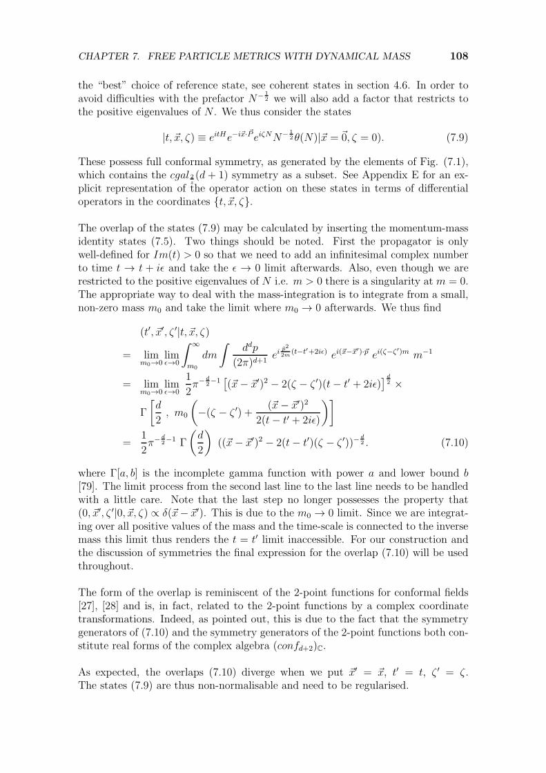
CHAPTER 7. FREE PARTICLE METRICS WITH DYNAMICAL MASS 108
the “best” choice of reference state, see coherent states in section 4.6. In order toavoid difficulties with the prefactor N− 1
2 we will also add a factor that restricts tothe positive eigenvalues of N . We thus consider the states
|t, ~x, ζ) ≡ eitHe−i~x·~PeiζNN− 12θ(N)|~x = ~0, ζ = 0). (7.9)
These possess full conformal symmetry, as generated by the elements of Fig. (7.1),which contains the cgal 2
z(d + 1) symmetry as a subset. See Appendix E for an ex-
plicit representation of the operator action on these states in terms of differentialoperators in the coordinates t, ~x, ζ.
The overlap of the states (7.9) may be calculated by inserting the momentum-massidentity states (7.5). Two things should be noted. First the propagator is onlywell-defined for Im(t) > 0 so that we need to add an infinitesimal complex numberto time t → t + iǫ and take the ǫ → 0 limit afterwards. Also, even though we arerestricted to the positive eigenvalues of N i.e. m > 0 there is a singularity at m = 0.The appropriate way to deal with the mass-integration is to integrate from a small,non-zero mass m0 and take the limit where m0 → 0 afterwards. We thus find
(t′, ~x′, ζ ′|t, ~x, ζ)
= limm0→0
limǫ→0
∫ ∞
m0
dm
∫ddp
(2π)d+1ei
p2
2m(t−t′+2iǫ) ei(~x−~x′)·~p ei(ζ−ζ′)m m−1
= limm0→0
limǫ→0
1
2π− d
2−1[(~x− ~x′)2 − 2(ζ − ζ ′)(t− t′ + 2iǫ)
]d2 ×
Γ
[d
2, m0
(−(ζ − ζ ′) +
(~x− ~x′)2
2(t− t′ + 2iǫ)
)]
=1
2π− d
2−1 Γ
(d
2
)((~x− ~x′)2 − 2(t− t′)(ζ − ζ ′))−
d2 . (7.10)
where Γ[a, b] is the incomplete gamma function with power a and lower bound b[79]. The limit process from the second last line to the last line needs to be handledwith a little care. Note that the last step no longer possesses the property that(0, ~x′, ζ ′|0, ~x, ζ) ∝ δ(~x− ~x′). This is due to the m0 → 0 limit. Since we are integrat-ing over all positive values of the mass and the time-scale is connected to the inversemass this limit thus renders the t = t′ limit inaccessible. For our construction andthe discussion of symmetries the final expression for the overlap (7.10) will be usedthroughout.
The form of the overlap is reminiscent of the 2-point functions for conformal fields[27], [28] and is, in fact, related to the 2-point functions by a complex coordinatetransformations. Indeed, as pointed out, this is due to the fact that the symmetrygenerators of (7.10) and the symmetry generators of the 2-point functions both con-stitute real forms of the complex algebra (confd+2)C.
As expected, the overlaps (7.10) diverge when we put ~x′ = ~x, t′ = t, ζ ′ = ζ .The states (7.9) are thus non-normalisable and need to be regularised.

CHAPTER 7. FREE PARTICLE METRICS WITH DYNAMICAL MASS 109
7.3 The Gravitational Dual of the Dynamical
Mass Free Particle
We are now in a position to investigate possible dual gravitational descriptions ofthe Schrodinger algebra Hamiltonians with dynamical mass. We will here workwith the free particle but, as before, another choice of Hamiltonian (from the con-formal Galilei algebra) will only entail a coordinate transformation. We can recoverregularised states from (7.9) by complexifying all the coordinates
t → τ ≡ t+ iβ ; ~x → ~z ≡ ~x+ i~y ; ζ → θ ≡ ζ + iα. (7.11)
We may derive the Kahler potential by simply complexifying the coordinates in theoverlap (7.10) and taking its logarithm. The inclusion of complex time, β > 0, in factmakes the integrals in the derivation of (7.10) more well-behaved and the calculationcarries through without alteration. As an example we give here the metric for d = 1
ds2 =1
2(y2 − 2αβ)2
(α2(dt2 + dβ2) +
y2 + 2αβ
2(dx2 + dy2) + β2(dζ2 + dα2)
−yα(dβdy + dydβ + dtdx+ dxdt)− yβ(dydα+ dαdy + dxdζ + dζ)
+y2
2(dβdα+ dαdβ + dtdζ + dζdt)
)(7.12)
The higher dimensional manifolds look very similar with the y’s and x’s replacedby the appropriate vectors (and dot products added). It may be verified that thesemanifolds (for any d) are Einstein and the scalar curvature is constant R = −72
d.
This implies that the expectation values of symmetry generators satisfy (6.5) i.e.
∇2Φ = − R
d+ 2Φ. (7.13)
The Killing vectors, which are the vector fields related to these expectation value(5.4) close on the algebra of Fig. (7.1). The Laplacian commutes will all the Killingvectors and is a second order differential operator. It must thus be a differentialoperator representation of the Casimir.
We are only considering the trace of the field equations in (7.13). Though themetric (7.12) is Einstein with constant scalar curvature it is not conformally flatand thus the Weyl tensor is still non-zero. As explained we may consider this onefield equation (7.13) if we add more boundary conditions. We will do this explicitlyfor this example.
The expectation values of the symmetry generators are not the only solutions of(7.13), however. This is a consequence of the fact that we are only considering thetrace of the field equations. We have to specify additional boundary conditions inorder for the field equation solution to be that of the desired expectation value.
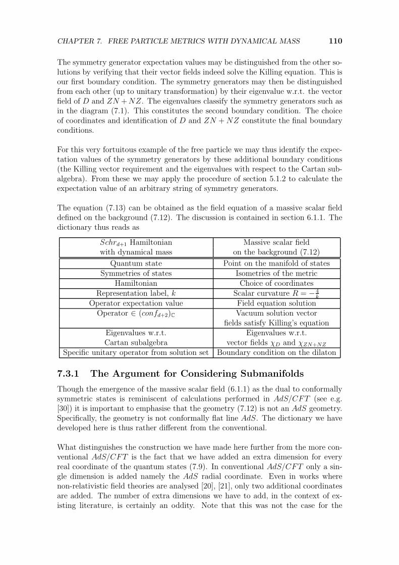
CHAPTER 7. FREE PARTICLE METRICS WITH DYNAMICAL MASS 110
The symmetry generator expectation values may be distinguished from the other so-lutions by verifying that their vector fields indeed solve the Killing equation. This isour first boundary condition. The symmetry generators may then be distinguishedfrom each other (up to unitary transformation) by their eigenvalue w.r.t. the vectorfield of D and ZN +NZ. The eigenvalues classify the symmetry generators such asin the diagram (7.1). This constitutes the second boundary condition. The choiceof coordinates and identification of D and ZN +NZ constitute the final boundaryconditions.
For this very fortuitous example of the free particle we may thus identify the expec-tation values of the symmetry generators by these additional boundary conditions(the Killing vector requirement and the eigenvalues with respect to the Cartan sub-algebra). From these we may apply the procedure of section 5.1.2 to calculate theexpectation value of an arbitrary string of symmetry generators.
The equation (7.13) can be obtained as the field equation of a massive scalar fielddefined on the background (7.12). The discussion is contained in section 6.1.1. Thedictionary thus reads as
Schrd+1 Hamiltonian Massive scalar fieldwith dynamical mass on the background (7.12)
Quantum state Point on the manifold of statesSymmetries of states Isometries of the metric
Hamiltonian Choice of coordinatesRepresentation label, k Scalar curvature R = − 4
k
Operator expectation value Field equation solutionOperator ∈ (confd+2)C Vacuum solution vector
fields satisfy Killing’s equationEigenvalues w.r.t. Eigenvalues w.r.t.Cartan subalgebra vector fields χD and χZN+NZ
Specific unitary operator from solution set Boundary condition on the dilaton
7.3.1 The Argument for Considering Submanifolds
Though the emergence of the massive scalar field (6.1.1) as the dual to conformallysymmetric states is reminiscent of calculations performed in AdS/CFT (see e.g.[30]) it is important to emphasise that the geometry (7.12) is not an AdS geometry.Specifically, the geometry is not conformally flat line AdS. The dictionary we havedeveloped here is thus rather different from the conventional.
What distinguishes the construction we have made here further from the more con-ventional AdS/CFT is the fact that we have added an extra dimension for everyreal coordinate of the quantum states (7.9). In conventional AdS/CFT only a sin-gle dimension is added namely the AdS radial coordinate. Even in works wherenon-relativistic field theories are analysed [20], [21], only two additional coordinatesare added. The number of extra dimensions we have to add, in the context of ex-isting literature, is certainly an oddity. Note that this was not the case for the
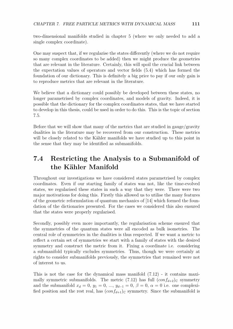
CHAPTER 7. FREE PARTICLE METRICS WITH DYNAMICAL MASS 111
two-dimensional manifolds studied in chapter 5 (where we only needed to add asingle complex coordinate).
One may suspect that, if we regularise the states differently (where we do not requireso many complex coordinates to be added) then we might produce the geometriesthat are relevant in the literature. Certainly, this will spoil the crucial link betweenthe expectation values of operators and vector fields (5.4) which has formed thefoundation of our dictionary. This is definitely a big price to pay if our only gain isto reproduce metrics that are relevant in the literature.
We believe that a dictionary could possibly be developed between these states, nolonger parametrised by complex coordinates, and models of gravity. Indeed, it ispossible that the dictionary for the complex coordinates states, that we have startedto develop in this thesis, could be used in order to do this. This is the topic of section7.5.
Before that we will show that many of the metrics that are studied in gauge/gravitydualities in the literature may be recovered from our construction. These metricswill be closely related to the Kahler manifolds we have studied up to this point inthe sense that they may be identified as submanifolds.
7.4 Restricting the Analysis to a Submanifold of
the Kahler Manifold
Throughout our investigations we have considered states parametrised by complexcoordinates. Even if our starting family of states was not, like the time-evolvedstates, we regularised these states in such a way that they were. There were twomajor motivations for doing this. Firstly this allowed us to utilise the many featuresof the geometric reformulation of quantum mechanics of [14] which formed the foun-dation of the dictionaries presented. For the cases we considered this also ensuredthat the states were properly regularised.
Secondly, possibly even more importantly, the regularisation scheme ensured thatthe symmetries of the quantum states were all encoded as bulk isometries. Thecentral role of symmetries in the dualities is thus respected. If we want a metric toreflect a certain set of symmetries we start with a family of states with the desiredsymmetry and construct the metric from it. Fixing a coordinate i.e. consideringa submanifold typically excludes symmetries. Thus, though we were certainly atrights to consider submanifolds previously, the symmetries that remained were notof interest to us.
This is not the case for the dynamical mass manifold (7.12) - it contains maxi-mally symmetric submanifolds. The metric (7.12) has full (confd+2)C symmetryand the submanifold xd = 0, y1 = 0, ..., yd−1 = 0, β = 0, α = 0 i.e. one complexi-fied position and the rest real, has (confd+1)C symmetry. Since the submanifold is
CHAPTER 7. FREE PARTICLE METRICS WITH DYNAMICAL MASS 112
d+ 2-dimensional it is maximally symmetric.
In the sections that follow we will show some of the interesting submanifolds of(7.12) that are studied in the literature. In deriving them we will present twoperspectives. First we will show how the metrics of the submanifolds may be con-structed explicitly from quantum states. This will identify the dual quantum states(and thus specifically the boundary states) of these existing works explicitly. Secondwe will derive these metrics by restricting the Kahler manifold to a submanifold.We believe that this second perspective is key to furthering the higher dimensionaldictionaries in a systematic way, our topic of discussion in section 7.5.
7.4.1 The Maximally Symmetric Submanifold
To emphasise its importance and its role as the radial coordinate on the submanifoldswe now relabel yd → r. We first consider the maximally symmetric submanifold.The submanifold metric may be constructed from the states
|r, t, ~x, ζ) ≡ e−rPdeitHei~x·~PeiζNN− 1
2θ(N)|~x = ~0, ζ = 0) (7.14)
where r 6= 0 and the components of ~P run from 1 to d − 1. These states onlyhave one additional coordinate (compared to (7.9)) for regularisation and possessthe full set of symmetries generated by the operators in the root diagram, Fig. (7.1)dimension d + 1 i.e. (confd+1)C. The overlap of these states can be calculated, inidentical fashion to (7.10), as
(r′, t′, ~x′, ζ ′|r, t, ~x, ζ) = 1
2π− d
2−1 Γ
(d
2
)(−(r+ r′)2 + (~x− ~x′)2 − 2(t− t′)(ζ − ζ ′))−
d2 .
(7.15)Using the overlap (7.15) we find the metric
ds2 =d
4r2(dr2 − d~x2 + dtdζ). (7.16)
As mentioned, this d + 2-dimensional metric possess 12(d + 2)(d + 3) isometries so
that it is maximally symmetric. This, together with its negative scalar curvature,implies that this manifold is AdSd+2.
The calculation from (7.14) is a direct calculation of the metric (7.16) from thefamily of quantum states. It is useful to think from another perspective namelythat the metric (7.16) is the metric of a submanifold of the Kahler manifold (7.12).It is the xd = 0, y1 = 0, ..., yd−1 = 0, β = 0, α = 0 submanifold of (7.12).
7.4.2 The z = 2-Symmetric Metrics
The symmetry of (7.16) is conformal. If we are interested in metrics that onlypossess a smaller set of symmetry, e.g. only the Schrodinger symmetry, we have torestrict the dynamical symmetry in some way. We define
|r, t, ~x, ζ)α = e−rPdeitHei~x·~PeiζNe−αNN− 1
2 θ(N)|~x = ~0, ζ = 0) (7.17)

CHAPTER 7. FREE PARTICLE METRICS WITH DYNAMICAL MASS 113
where we do not consider α as a coordinate. It is thus only a parameter and fulfilsthe role of a symmetry filter, similar to the role played by the density matrix insection 3.4.1. The rationale for doing this is that only the Schr(d) operators ofFig (7.1) commute with N , see Fig. (7.1). The factor of e−αN thus breaks all theundesired conformal symmetries. The overlap can be calculated using the steps in(7.10) and is given by
α(r′, t′, ~x′, ζ ′|r, t, ~x, ζ)α
=π− d
2−1
2Γ
(d
2
)(−(r + r′)2 + (~x− ~x′)2 − 2(t− t′)(ζ − ζ ′ + 2iα)
)− d2 (7.18)
which produces the metric
ds2 =d
4r2(dr2 − d~x2 + dtdζ) +
dα2
2r4dt2. (7.19)
This is, up to rescaling of the coordinates and a change of signature, precisely themetric studied by [20] and [21] for z = 2. The procedure we have employed here ispretty much identical to that of [21] namely to start from something with full con-formal symmetry and break it in an appropriate way to only retain the Schrodingersymmetry. In their study the symmetries are broken on the level of the metric whilehere we provide the analogous procedure on the level of the quantum states.
The resulting metric (7.19) is, of course, already known so that it does not present anew result itself. What we have managed to do with the construction is to providean explicit and systematic procedure to construct these metrics from the quantumstates of the free particle. This strengthens the dictionary developed by these worksand allows us to test aspects of this dictionary very directly. As an example of thiswe provide our own perspective on the apparent two additional dimensions which isa novelty of this AdS/NRCFT correspondence.
As is stated in [20] the additional dimension ζ is the conjugate mass. Unlike theconventional wisdom of AdS/CFT the regularisation parameter r is not associatedwith an energy scale but rather with a length scale. The reason for the two addi-tional dimensions (when comparing the d + 2-dimensional manifold to the schr(d)algebra) is also very clear - the Schrodinger algebra in d dimensions needs to beviewed, in this construction, as a subalgebra of the d + 1 dimensional conformalalgebra after introducing the conjugate mass. To the conformal algebra one mayadd, in line with the standard wisdom, one additional dimension to regularise themetric in the bulk. These two steps then comprise the apparent two dimensions oneneeds to add to the non-relativistic theory.
We may once more view the metric (7.19) as being constructed directly from thequantum states (7.17) or simply as the metric on a submanifold of the Kahler mani-fold (7.12). Here it is the xd = 0, y1 = 0, ..., yd−1 = 0, β = 0, α = fixed but non-zeroslice of the Kahler manifold (7.12).
CHAPTER 7. FREE PARTICLE METRICS WITH DYNAMICAL MASS 114
7.4.3 The z 6= 2 Symmetric Metrics
The z 6= 2 conformal Galilei algebra (7.1) is another subalgebra of the complexconformal algebra. An important difference to the z = 2 algebra is that the specialconformal generator, K, is not included. We may again alter the states appropriatelyin order to filter out only the conformal Galilei symmetry as dynamical symmetry.From the states (7.17) we have to filter out the special conformal symmetry gener-ated by K.
In order to break the special conformal symmetry of (7.17) it is useful to under-stand exactly why the states still possess special conformal symmetry. The factore−rPd in (7.17) commutes will all the position, momentum and rotation operatorsand with H . The operators D and K are thus the only Schrodinger algebra genera-tors that induce non-trivial transformations on r. If we thus change the factor eαNto eαf(r)N we could thus break the D (scaling) and K (special conformal) symmetry.We must pick f(r) in such a way that it breaks the special conformal symmetry butretains the scaling symmetry. We thus make the ansatz for the states
|r, t, ~x, ζ)αr = e−rPdeitHei~x·~PeiζNe−αr2−zNN− 1
2 θ(N)|~x = ~0, ζ = 0). (7.20)
Following the step of (7.10) this leads to the overlap
αr(r′, t′, ~x′, ζ ′|r, t, ~x, ζ)αr
=(−(r + r′)2 + (~x− ~x′)2 − 2(t− t′)(ζ − ζ ′ + iα(r2−n + r′2−n)
)− d2 (7.21)
and then the metric
ds2 =d
4r2(dr2 − d~x2 + dtdζ) +
dα2
2r2zdt2. (7.22)
This is the metric studied by [20] for arbitrary z and is symmetric under the cgal 2z(d)
transformations.
Once more the metric (7.22) may be viewed as the metric of a submanifold of theKahler manifold (7.12), but one where the slice is now dependent on the AdS radialcoordinate. Specifically we have to consider the xd = 0, χ1 = 0, ..., χd−1 = 0, β = 0,α = α′r2−z submanifold.
7.4.4 Discussion of the Submanifold Metrics
In the works [20], [21], [34] the metrics are taken as the starting point to their anal-ysis which involves the calculation of the correlation functions. Their calculationsinvariably involve considering the massive scalar field on the background of interestand applying the conventional AdS/CFT dictionary i.e. that the functional deriva-tive with respect to the boundary value of the fields yields the correlation functions.
In the dictionaries we have developed for the families of states with complex co-ordinates this is, of course, not the interpretation we have attached to the fields. In

CHAPTER 7. FREE PARTICLE METRICS WITH DYNAMICAL MASS 115
our dictionaries the fields are interpretable directly as the expectation values of oper-ators. It thus seems that in order to recast the works [20], [21], [34] in the mould of asystematic set of tools we will have to undertake the study of a whole new dictionary.
Nonetheless, the fact that we could derive the metrics (7.16), (7.19) and (7.22) sys-tematically, starting from a family of quantum states achieves two things. Firstly, itsupplements these works by identifying the quantum states on the boundary explic-itly and makes clear the interpretations of the coordinates and the scalar curvature.
Secondly, it hints that a systematic construction of these dual systems may, infact be possible. This will certainly require a lot of additional work, but we believethat this can be done. In the final section of this chapter we will discuss a possiblestrategy for doing this that utilises the existing dictionaries for the complex coor-dinate states. We warn the reader that this is simply speculation and must not beviewed as a rigorous discussion.
7.5 Dictionary on the Submanifold?
The two perspectives on the metrics we have constructed in this chapter is to eitherconstruct them explicitly from the quantum states or consider the metric as themetric of a submanifold of a Kahler metric. It can be summarised in diagrammaticform as follows
Family of States,Complex coordinates
|z1, ..., zn)
(Kahler GeometryExisting Dictionary
)
(Family of States
|s1, ..., sm)
) (Metric of Lower DimensionNo Current Dictionary
)fixed coordinates submanifold
The important observation is that we have an existing dictionary for the complexcoordinate states and the Kahler geometry. As discussed, the expectation values ofoperators are intricately linked to vector fields on the manifold in this case. Thisformed the basis of the dictionaries we developed.
The submanifold is not necessarily Kahler so that this very useful relation no longerholds. However, it is useful to recall what quantities we are interested in. Our goal isto calculate the expectation value of an arbitrary string of operators. Suppose thenwe are given a family of states |~s) that can be obtained from a family of states ofcomplex coordinates |~z) by fixing some its coordinates. Suppose further that we wishto calculate the expectation values of some string of operators Φ = 〈~s|A1, ..., Aj|~s〉.
We cannot at this point say anything regarding the equations of motion for Φ.
CHAPTER 7. FREE PARTICLE METRICS WITH DYNAMICAL MASS 116
What we have derived are the equations of motion for Φ′ = 〈~z|A1, ..., Aj|~z〉 in sec-tion 6.1. Though there is certainly some work still needed to deal with the full setof equations of motion (which entails understanding the role played by the Weyltensor) this should be possible for these complex coordinates.
What one will have to do, in order to write down the appropriate equations ofmotion for Φ, is to take the equations of motion for Φ′ and restrict these to the sub-manifold. One should then be able to recover the appropriate equations of motionfor Φ from these and then try to match them up to an appropriate theory of grav-ity. This is certainly an avenue of future research that begs pursuing after which,hopefully, one may start to develop systematic dictionaries for the dual of quantumsystems and theories of gravity where the metric is given by (7.19), for instance.
7.6 Discussion
Our investigations in this chapter has met with partial success. By considering thecentral extension of the Schrodinger algebra (the mass) as a dynamical variable wewere able to sidestep some of the difficulties we encountered in chapter 6 for thehigher dimensional duals. The field equations were simple enough that we couldpackage them in a simple dictionary involving the massive scalar field.
One stumbling block that remains is that the manifolds are not conformally flatwhich adds terms to the equations of motion. This can be remedied by only consid-ering one field equation - the trace of the field equations - which has no contributionfrom the Weyl tensor. The discarded field equations have to be substituted withboundary conditions.
The dictionary departs from the conventional gauge/gravity duality in that thebulk dimensions are numerous and not just one or two. We identified that sub-manifolds of these Kahler manifolds are precisely the manifolds investigated in theliterature [20], [21] in the context of the AdS/NRCFT and we also identified an AdSsubmanifold. Our construction thus recovers the metrics and supplements these ex-isting works by identifying the dual quantum mechanical states explicitly. However,because the properties we discussed in section 3.3 are no longer applicable on thesesubmanifolds, we could not, as yet, develop a systematic, working dictionary.
We concluded the chapter with a speculative discussion of how one may proceedto develop such a dictionary. Two ingredients for this development will prove es-sential - firstly understanding how the equations of motion may be restricted toa submanifold and secondly, understanding not just the trace of the equations ofmotion but the full set. The reason for this is simple - the Weyl tensor contributionson the submanifold may be significantly less complex. The full set of field equa-tions may thus be tractable on the submanifold, though they are not on the Kahlermanifold. We hope to address these questions in future.

Chapter 8
Conclusion and Outlook
In this thesis we managed to develop a systematic procedure to repackage a givenquantum mechanical model as a semi-classical theory of gravity. The most impor-tant part of this construction was the identification of a metric - a way to build ageometry from a given family of quantum states. The construction we chose wasrelatively easy to work with but also ensured that the dynamical symmetries areencoded as isometries of the metric and anti-symmetric two-form.
Many aspects of this construction, before theories of gravity even enter the dis-cussion, are intriguing for the purposes of the AdS/CFT correspondence. For non-normalisable reference states it is necessary to regularise the quantum states by somemeans. This gives rise, naturally, to the idea of a bulk, where the states are normal-isable, and a boundary where the original non-normalisable states are defined. Inthe case of time-evolved states (with complexified time), an asymptotically anti-deSitter geometry results very generally. In addition, the AdS2 radial coordinate hasthe interpretation of an energy scale.
We showed that in the case of normalisable reference states the resulting metriccan be much more general. In particular the SU(2) coherent states and Glaubercoherent states resulted in de Sitter and flat space metrics respectively. Thoughthese geometries were not studied in the same detail as the AdS examples they are,especially in two dimensions, a topic of future research that may yield interestingresults in the context of, for instance, the dS2/CFT1 correspondence.
The procedure from the geometry to the dual gravitational description is not asclear cut precisely because there are several ways in which to do this. One es-sentially has to make the first few entries in the quantum mechanics / theory ofgravity dictionary - a choice that determines the dictionary one will develop sub-sequently. The investigation of choices other than the one we made can well leadto other interesting dictionaries. For the sake of simplicity we proposed that metricand expectation values of operators should be associated with the metric and fieldsthat solve the field equations of some model of gravity. After using some resultsfrom section 3.3 we managed to write down a set of equations of motion for theexpectation values of operators (with respect to complex coordinate states). The
117

CHAPTER 8. CONCLUSION AND OUTLOOK 118
gravitational action should thus be chosen so that its field equations are the sameas these equations of motion.
Though this was a simple choice, it met with success for especially the two-dimensionalmanifolds. When we focused on the SU(1, 1) Hamiltonian models, which all producean AdS2 geometry, we were able to provide clarity to and extend the AdS2/CFT1correspondence proposed in [13]. We could identify the quantum states of the AdS2
dual explicitly, provide the mapping between quantum state and geometry (and viceversa) and clarify some of the puzzles they discuss in their work. Specifically, wecould explain why the appropriate form of the 2- and 3-point correlation functionsare produced despite the quantum states being non-normalisable and despite theabsence of a conformally invariant state in the Hilbert space. We showed that thisis simply a consequence of the dynamical symmetries.
We went beyond this correspondence of [13], which is roughly a dual between thegeometry of AdS2 and CFT1 and thus devoid of gravitational content, and identifiedthe model of dilaton gravity as our appropriate gravitational dual. As it turns out,this model features prominently in the context of the AdS2/CFT1 correspondence[15]-[19]. Since our construction is systematic and explicit we have direct accessto the quantum mechanics / dilaton gravity dictionary. This enabled us to fill insome details of these existing works pertaining to the interpretation of the dilaton,the interpretation of the dilaton black hole mass, the explicit quantum mechanicalmodel on the boundary and the scalar curvature. Also, we were able to extend to thedual description of operators that are not generators of symmetry. Of significanceis how natural the analysis follows from our construction. This holds the promise ofgeneralisations to models that do not possess so many symmetries.
We concluded with an explicit dictionary between conformal quantum mechanicsand 2d JT-model dilaton gravity. We showed that the correct expression for theentropy of the dilaton gravity black hole can be recovered by simply considering theconformal transformations of the model. Our analysis here is still qualitative in thatwe need address issues pertaining to the appropriate normalisation of the dilaton.
We also briefly looked at the SU(2) Hamiltonians which are dual to theories onde Sitter space. We showed here that the values of operators can be recovered inthe dual gravitational description in an almost identical way to the SU(1, 1) calcu-lation. The Glauber coherent states, which produce a flat space geometry, were alsoconsidered. We commented that the Glauber coherent states are thus best servedas a large j limit of the SU(2) coherent states.
Our attention moved, in the last two chapters, to the higher dimensional duals.Our results here are less developed than the two-dimensional examples we exploredpreviously. The procedure and considerations for constructing a dual in higher di-mensions are identical to the two-dimensional case. A calculational difficulty is thatthe Riemann curvature tensor (which determines the equations of motion) for Kahlermanifolds always has a non-zero Weyl tensor. This adds terms into the equations of
CHAPTER 8. CONCLUSION AND OUTLOOK 119
motion that we do not yet know how to handle generally. The treatment of theseterms is, of course, an important avenue of future study. We thus made a sensiblesimplification as a first step - we consider only the trace of the equations of motionand consign the information of the other equations of motion to additional bound-ary conditions. We identified the massive scalar field as a model that produces theappropriate field equation.
The natural generalisation of the su(1, 1) coherent states to the higher-dimensionalcase is to add position. This extension to the higher-dimensional case caused aproblem. The Killing vectors do not close on the Schrodinger algebra because one ofthe operators of the algebra only generates phase shifts of the quantum states. Itsassociated Killing vector is thus zero. Despite this we managed to develop a schemefor calculating the expectation values of operators. Understanding the algebraiccontent of the Laplace operator will give great insight into this matter. This wepostpone to future study.
The situation is a lot more favourable if one considers the central extension ofthe Schrodinger algebra (the mass) as dynamical. This allows us to enlarge theSchrodinger algebra to a real form of the complex conformal algebra. The Killingvectors are now a differential operator representation of the algebra and the analysiscan be done more simply.
Unlike its two-dimensional counterpart these higher dimensional duals do not re-semble many similar works in the literature. The primary reasons for this are thatan AdS geometry cannot be achieved and that there are more than one additionaldimensions. The lack of comparable examples in the literature is precisely why thiscase is not investigated to the same level of detail as its two-dimensional counter-part. For this case we did provide a simple dictionary.
At first glance it may appear as if this construction for the higher dimensions,though possessing a sensible and systematic dictionary, departs from the traditionalAdS/CFT approach too much to provide insight therein. However, we showed ex-plicitly that several important metrics, often the starting point of analysis e.g. [20],[21], [34], are easily identifiable submanifolds of the Kahler manifold. We thus sup-plemented their study by identifying the quantum states on the boundary explicitly,providing the explicit origins of the extra dimensions and an interpretation for thescalar curvature. In terms of the question of establishing a gravitional dual (as op-posed to just calculating the metrics) we currently have no answer. Since we losethe Kahler structure on the submanifold we also lose the dictionary we have devel-oped throughout the rest of the thesis. We proposed that it is possible that onemay utilise the Kahler dictionary to learn from the dictionary on the submanifold.Developing this submanifold dictionary is, in the opinion of the writer, the mostpressing question that emerges from the investigation in this thesis.
As was mentioned in the introductory section of this thesis, the power of the con-struction does not lie in its ability to mimic all the aspects of the gauge/gravity

CHAPTER 8. CONCLUSION AND OUTLOOK 120
duality but rather in its systematic nature. It is the hope of this author that thiswork and its future generalisations can create a systematic framework in which someexamples of the gauge/gravity duality may be investigated directly.

Appendices
121
Appendix A
The Geometric Quantities ofRelevance
In this thesis we will construct a metric and anti-symmetric two-form from a familyof quantum states and match these to a semi-classical theory of gravity in some way.The curvature properties of these metrics, as one would expect, play a key role andwe define all the quantities used in the thesis in this appendix. A good reference forthe formulas provided here is [71].
Whenever tensor indices are used a chosen geometry is implicitly defined. Themetric tensor gµν is used to raise and lower indices of tensors e.g.
yµ = gµαyα (A.1)
where, also throughout the thesis, the Einstein summation convention is used i.e.repeated indices are summed over. We have illustrated it in (A.1) for a vector butit is true of any tensor index. The covariant derivative of a vector field xµ is definedas
∇νxµ ≡ ∂νx
µ + xαΓµαν ; ∇νxµ ≡ ∂νxµ − xαΓ
αµν (A.2)
where Γαµν are the Christoffel symbols of the second type defined as
Γαµν ≡ 1
2gαβ (∂µgβν + ∂νgβµ − ∂βgµν) . (A.3)
The covariant derivative has the interpretation of how a given vector field changesas its transported around the manifold. The Christoffel symbol part (A.2) indi-cates that it may also change orientation if the geometry is curved. Note that, bydefinition, we have that
∇µgαβ = ∇µgαβ = ∇µg
αβ = 0 (A.4)
i.e. the metric tensor is compatible with the covariant derivative. Indeed, techni-cally, metric compatibility or incompatibility defines the covariant derivative andnot the other way around. Throughout the thesis we use the compatible definitionof the covariant derivative.
122
APPENDIX A. THE GEOMETRIC QUANTITIES OF RELEVANCE 123
The Riemann curvature tensor, R βµνα , is defined as
(∇µ∇ν −∇ν∇µ)xα ≡ R βµνα xβ (A.5)
and has the interpretation of by how much the orientation of a vector is going to differif one moves it from point A to point B, infinitesimally close to one another, alongtwo different paths. The curvature tensor (A.5) contains all curvature informationof the manifold. It can be shown that the curvature tensor possesses the followingsymmetries
Rµναβ = −Rνµαβ = −Rµνβα = Rαβµν . (A.6)
Consequently there is only one unique, non-trivial contraction of the Riemann tensor
Rµν = Rαµαν (A.7)
which is the Ricci tensor. It certainly contains less curvature information than theRiemann tensor but contains sufficient information for some physical applicationssuch as in the Einstein field equations. The scalar curvature is defined as the traceof the Ricci tensor
R = Rαα (A.8)
while an Einstein manifold has the property that the Ricci tensor is proportional tothe metric i.e.
Rµν =R
dgµν (A.9)
where d is the dimension of the manifold. Note that this does not imply that thescalar curvature is necessarily constant.
It can be shown that all two-dimensional (d = 2) metrics are Einstein (A.9) whileall three-dimensional metrics satisfy
Rαβγδ = (Rαγgβδ +Rβδgαγ − Rαδgβγ − Rβγgαδ)−R
2(gαγgβδ − gαδgβγ). (A.10)
These identities make the 2- and 3-dimensional case quite novel. For higher dimen-sions one has that
Rαβγδ = Wαβγδ
+1
n− 2(Rαγgβδ +Rβδgαγ − Rαδgβγ −Rβγgαδ)
− R
(n− 1)(n− 2)(gαγgβδ − gαδgβγ) (A.11)
whereWαβγδ is the Weyl tensor, which contains information pertaining the conformalproperties of the metric. If the metric is conformally flat i.e. gµν = f(x1, x2, ..., xd)δµνthen the Weyl tensor is zero. Two- and three-dimensional metrics are thus alwaysconformally flat while the two-dimensional metrics are in addition Einstein metrics.These simplifications will prove useful in the analysis in the thesis.

Appendix B
Field Equations for Einstein- andDilaton Gravity
B.1 Einstein Gravity
See the works [56], [80] and [81] for good discussions on Einstein gravity i.e. generalrelativity. In this thesis we will be primarilly interest in the action derivation ofthe field equations. We start with the Einstein-Hilbert action (with cosmologicalconstant included)
SEH =
∫ddx
√−g (R − 2Λ + LM). (B.1)
Here g is the determinant of the metric, R is the scalar curvature, Λ the cosmologicalconstant and LM the matter content. The field equations can be derived from (B.1)by varying the action with respect to the inverse metric i.e.
1√−gδSEH
δgµν= 0 =
1√−g
∫ddx
(δ(√−gR)δgµν
− 2Λδ√−gδgµν
+δ(√−gLM)
δgµν
)(B.2)
where the factor of 1√−gis for convenience. Note that we have are taking a functional
derivative. In order to avoid confusion we make the following remark. The functionalderivative act on functionals such as the action. Whenever we write
δ
δf(x)
∫dx′F (f(x′)) =
∫dx′
δF (f(x′))
δf(x)(B.3)
we mean∫dx′
δF (f(x′))
δf(x)=
∫dx′∂fF (f(x
′))δ(x− x′) = ∂fF (f(x)). (B.4)
In other words, the functional derivative on a function introduces a delta functionwhich is integrated out. Typically when a term is begin integrated over we use thenotation for functional derivatives but if not we use the notation of partial derivative.
124

APPENDIX B. FIELD EQUATIONS FOR EINSTEIN- AND DILATON GRAVITY125
Returning to the field equations of (B.2) we first require
∂√−g∂gµν
=1
2√−g
∂(−g)∂gµν
= − 1
2√−g
∂ det (gµν)
∂gµν
= − 1
2√−g
∂ det−1 (gµν)
∂gµν=
1
2√−g det2 (gµν)
∂ det (gµν)
∂gµν. (B.5)
In order to present the derivation as cleanly as possible we temporarily substitute thevariation of the metric as ∂gµν ≡ aµν . By now using properties of the determinantwe have that
det (gµν + aµν) = det (gµα) det (δνα + gαβaβν)
= det (gµα) exp(tr(ln(δνα + gαβa
βν)))
= det (gµα) exp(tr(gαβa
βν) +O(a2))
= det (gµα)(1 + det (gµν)tr(gαβa
βν) +O(a2))
= det (gµα) + det (gαβ)gµνaµν
⇒ ∂ det(gµν) = det (gαβ)gµνaµν = det (gαβ)gµν∂g
µν (B.6)
where we have used the fact that det(gµν) = det(gαβ) since it is merely a relabeling.By now combining (B.5) and (B.6) we find that
1√−g∂√−g∂gµν
=gµν
2(−g) det(gµν) =ggµν2(−g) = −1
2gµν . (B.7)
This result is the same for any signature of the metric. We have derived it here for|g| = −g but an almost identical derivation can be done for |g| = g. Using this wenow define the energy momentum tensor Tµν as
− Tµν ≡ 1√−g∂(√−gLM )
∂gµν=
1√−gδ√−g∂gµν
LM +∂LM
∂gµν= −1
2gµνLM +
∂LM
∂gµν. (B.8)
The last bit we need to complete the field equations (from (B.2)) is the partialderivative of the scalar curvature
∂(√−gR)∂gµν
=∂(gαβRαβ)
∂gµν= Rµν + gαβ
∂Rαβ
∂gµν(B.9)
which we will be handling slightly differently. The Ricci scalar is given by tracingover indices of the Riemann tensor which in turn is given in terms of the Christoffelsymbols
Rµν = Rαµαν ; Rα
µβν = ∂βΓαµν − ∂νΓ
αµβ + Γα
βλΓλµν − Γα
νλΓλµβ . (B.10)
By applying the chain rule we calculate ∂Rµν
∂gµν= ∂Rµν
∂Γρµν
∂Γρµν
∂gµν. We will show that the
contribution of this term is merely a surface term so we will not calculate this

APPENDIX B. FIELD EQUATIONS FOR EINSTEIN- AND DILATON GRAVITY126
explicitly. Instead it will suffice to calculate ∂Rµν = Rµν(Γρµν+γ
ρµν)−Rµν(Γ
ρµν) where
γρµν ≡ δΓρµν is defined as the variation of the Christoffel symbol (and is assumed to
be small). We begin with
∂Rαµβν = ∂βγ
αµν − ∂νγ
αµβ + γαβλΓ
λµν + Γα
βλγλµν − γανλΓ
λµβ − Γα
νλγλµβ
=(∂βγ
αµν + Γα
βλγλµν − γανλΓ
λµβ
)−(∂νγ
αµβ + Γα
νλγλµβ − γαβλΓ
λµν
)
=(∂βγ
αµν + γλµνΓ
αβλ − γανλΓ
λµβ − γαµλΓ
λνβ
)
−(∂νγ
αµβ + γλµβΓ
ανλ − γαβλΓ
λµν − γαµλΓ
λνβ
)
= ∇βγαµν −∇νγ
αµβ (B.11)
from which it follows that
gµν∂Rµν = gµν(∂Rαµαν) = gµν∇αγ
αµν −∇νγ
αµα = ∇α(g
µνγαµν − gµαγβµβ). (B.12)
The metric is compatible with the covariant derivative (A.4). This should holdbefore as well as after the variation i.e.
∇σgµν = 0 = ∇′
σ(gµν + aµν) (B.13)
where aµν is assumed to be small and the covariant derivatives are varied as ∇σ →∇′
σ. The variation is assumed small so that we can derive, up to first order
∇σaµν = −gµλγνσλ − gλνγµσλ (B.14)
from which we can derive two identities
∇σgµνaµν = −2γασα
∇σaµσ = −gµλγσσλ − gλσγµσλ. (B.15)
By combining these
∇αgαλ∇λgµνa
µν −∇α∇σaασ = ∇α(g
µνγαµν − gαλγσλσ)
⇒ gµνδRµν = ∇α (gµν∇αaµν −∇σaασ) ≡ ∇αv
α. (B.16)
By inserting the explicit expressions (B.7), (B.8), (B.9), (B.16) into (B.2) we findthat
0 =1√−g
δSEH
δgµν= Rµν −
1
2Rgµν +Λgµν −Tµν +
∫ddx
√−g δ
δgµν∇av
a(δgµν). (B.17)
The integral over the divergence of a vector, by Stokes’ theorem, can yield at most aboundary term so that the integral does not contribute to the field equations. Theremainder of (B.17) is the Einstein field equations with cosmological constant.
B.2 Dilaton Gravity Field Equations
Another model of gravity that will be of interest is dilaton gravity [60]. In thesemodels we have included additional fields into the action which can change the fieldequations significantly. We will be interested in actions of the following form
S =
∫ddx
√−g (H(η)gµν∇µη∇νη +RD(η) + V (η, LM)) . (B.18)
APPENDIX B. FIELD EQUATIONS FOR EINSTEIN- AND DILATON GRAVITY127
For the field equations resulting from varying with respect to the metric we canapply the results above almost imediately
0 =1√−g
δS
δgµν
= D(η)
(Rµν −
1
2Rgµν
)+H(η)
(∇µη∇νη −
1
2gµνg
αβ∇αη∇βη
)
−1
2gµνV (η, LM) +
∂V (η, LM)
∂gµν
+1√−g
∫ddx
√−g δ
δgµν(D(η)∇αv
α) . (B.19)
The integral term is now no longer a simple divergence of a vector precisely becauseof the presence of the dilaton. This means we cannot apply Stokes’ theorem and itdoes not simply contribute a boundary term. Examining the integral more carefullyyields
1√−g
∫ddx
√−g δ
δgµν(D(η)∇αv
α)
=1√−g
∫ddx
√−g δ
δgµν(gµνD(η)∇2aµν −D(η)∇α∇σa
ασ)
which will produce a number of delta functions in the integral. The metric variationsaµν are contravariant and the gamma functions are thus added. Integrating by partswill keep the double derivatives unchanged but will switch the sign of the singlederivatives. This will correspond to a covariant derivative. This then implies that
1√−g
∫ddx
√−g δ
δgµν(D(η)∇αv
α) = gµν∇2D(η)−∇µ∇νD(η) (B.20)
so that we find the field equations also found in [57] after combining (B.19) and(B.20).
Of particular interest for the 2d models is the Jackiw-Teitelboim model which hasH [η] = 0 and D[η] = η and, due to two dimensions, Rµν = R
2gµν which yields the
field equations
− 1
2gµνV (η, LM) +
∂V (η, LM)
∂gµν+ gµν∇2η −∇µ∇νη = 0. (B.21)
Appendix C
Algebras That Feature in ThisThesis
In this appendix we summarise the various algebras that feature in the thesis. Westart with the Heisenberg algebra spanned by the operators P,X and I
[X,P ] = iI ; [X, I] = [P, I] = 0. (C.1)
The algebra can also be represented in terms of creation and annihilation operatorsa† = 1√
2(X + iP ) and a = 1√
2(X − iP ) which satisfies
[a, a†] = I ; [a, I] = [a†, I] = 0. (C.2)
Two of the special unitary groups will also be of importance. The su(2) algebrareads
[Jz, J±] = ±J± ; [J+, J−] = 2Jz (C.3)
and may be expressed in terms of creation and annihilation operators as [82]
Jz = a†a− N
2; J+ =
√Na†
√1− a†a
N; J− =
√N
√1− a†a
Na (C.4)
where N is the related to the representation label, the lowest eigenvalue of Jz. Inthe N → ∞ limit it is clear that J+√
N→ a† and J−√
N→ a.
The su(1, 1) algebra reads
[H,D] = iH ; [K,D] = −iK ; [H,K] = 2iD. (C.5)
The Cartan-Weyl basis for the su(1, 1) algebra is given by
K0 =1
2(K +H) ; K± =
1
2(K −H)± iD
[K0, K±] = ±K± ; [K−, K+] = 2K0. (C.6)
The su(1, 1) and Heisenberg algebras may be combined to form the Schrodingeralgebra. This algebra derives its name from the generators of dynamical symmetryfor the free Schrodinger equation [43] and is the semi-direct sum of the su(1, 1)
128

APPENDIX C. ALGEBRAS THAT FEATURE IN THIS THESIS 129
algebra (C.5) and d copies of the Heisenberg algebra (C.1) (related by rotationoperators Mjk). The commutation relations are
[Xj , Pk] = −iδj,k ; [K,H ] = −2iD
[Pj , D] =i
2Pj ; [Xj, D] = − i
2Xj
[Pj , K] = iXj ; [Xj, H ] = −iPj
[K,D] = −iK ; [H,D] = iH
[Xj ,Mkl] = i(g0jkXl − g0jlXk) ; [Pj,Mkl] = i(g0jkPl − g0jlPk)
0 otherwise (C.7)
where g0kl is the flat space metric in arbitrary signature. In this thesis Euclideansignature is used i.e. g0kl = δkl.
The conformal Galilei algebra, cgal 2z(d+1), is a generalisation of the Schrodinger al-
gebra where one has included a dynamical exponent z. The algebra is also centrallyextended and reads
[Mij ,Mkl] = i(g0ikMjl + g0jlMik − g0ilMjk − g0jkMil)
[Gi,Mkl] = i(g0ikXl − g0ilKk) ; [Pi,Mkl] = i(g0ikPl − g0ilPk)
[Gi, Pj] = iδijN ; [D,Pi] = − i
2Pi
[D,Gi] =i
2(z − 1)Gi ; [D,N ] =
i
2(z − 2)N
[H,Gi] = −iPi ; [D,H ] = −z2iH (C.8)
where N is the central extension. The dynamical exponent z characterises the dif-ferent scaling behavior of time and position captured by the different scaling for Hand Gi.
The final algebra that is of importance is the conformal algebra given by
[D, Kµ
]= iKµ
[D, Pµ
]= −iPµ
[Pµ, Kν
]= 2iMµν − 2ig0µνD
[Kα, Mµν
]= i(g0αµKν − g0ανKµ)
[Pα, Mµν
]= i(g0αµPν − g0ανPµ)
[Mαβ , Mµν
]= i(g0αµMβν + g0βνMαµ − g0ανMβµ − g0βµMαν). (C.9)
In Appendix E it is shown that the conformal Gaililei algebra is a subalgebra of theconformal algebra of one dimension higher.
Appendix D
Baker-Campbell-HausdorffFormula
In this thesis the calculation of quantum state overlaps and transformation in-duced by a unitary transformation is critical. For this purpose the Baker-Campbell-Hausdorff formula [50], [51] is used extensively. In a nutshell the formula is usedto split an arbitrary group element as the product of a desired set of “basis” groupelements. In this appendix we show two examples of this formula that features inthis thesis.
D.1 BCH formula for the Heisenberg Group
The most well-known example of the BCH formula is its application to the Heisen-berg group. The relevant algebra is given in (C.1) and (C.2). Consider the followingHeisenberg algebra group element
U = eza†−za. (D.1)
This group element may be split as the product of the exponent of a creation operatorand the exponent of an annihilation operator as follows
eza†+za = eza
†
e−zae−12[za†,za] = eza
†
ezaeI2zz (D.2)
following (C.2). This expansion is possible precisely because [a†, a] = constant. Theexpansion (D.2) is particularly useful when the the group element (D.1) acts on thestate |0〉 annihilated by a. In this case
eza†−za|0〉 = eza
†
ezaeI2zz|0〉 = e
I2zzeza
† |0〉 (D.3)
so that the eza part of the expansion induces no transformation of |0〉. Anotheruseful example is if a Heisenberg group element acts on the state |x = 0) which issuch that X|x = 0) = 0. We then have that
eiaP+ibX |x = 0) = eiaP eibXe−12ab[P,X]|x = 0) = ei
ab2IeiaP |x = 0). (D.4)
130
APPENDIX D. BAKER-CAMPBELL-HAUSDORFF FORMULA 131
D.2 BCH formula for SU(1, 1)
As a second example we consider the BCH formulae for the SU(1, 1) group. Asimple way to derive the formula is to consider the 2 × 2 matrix representation ofSU(1, 1) given by
K+ =
(0 10 0
); K− =
(0 0−1 0
); K0 =
(12
00 −1
2
). (D.5)
It can be verified that the matrices (D.5) satisfies the correct commutation rela-tions (C.6). The BCH formula is representation independent so that, even thoughwe are considering a simple 2 × 2 matrix representation, the formula is valid forany representation. Given a general matrix element of SL(2) in the 2 × 2 matrixrepresentation (
α βγ δ
); αδ − βγ = 1 (D.6)
it may be broken up as(α βγ δ
)= exp
(β
δK+
)exp (−2 log (δ)K0) exp
(−γδK−
); δ 6= 0 (D.7)
= exp(−γαK−
)exp (2 log (α)K0) exp
(β
αK+
); α 6= 0.(D.8)
SU(1, 1) is a subgroup of SL(2) so that the above formulas holds for SU(1, 1) ele-ments also. As an application of the above we calculate the overlap of the harmonicoscillator states
|t) ≡ eit(H+ω2K)|x = 0) = eit(H+ω2K)e−K+ |0〉 (D.9)
where |0〉 is the state such that
K−|0〉 = 0 ; K0|0〉 = k (D.10)
where k is the representation label. The overlap of the states (D.9) is given by
(t′|t) = 〈0|e−K−ei(t−t′)(H+ω2K)e−K+|0〉. (D.11)
The SU(1, 1) element wedged between the states 〈0| and |0〉 may be split up using(D.7). The 2× 2 matrix representation of (D.11) is given by
e−K−ei(t−t′)(H+ω2K)e−K+
=
(cos(ω(t− t′)) + i(1+ω2) sin(ω(t−t′))
2ω− cos(ω(t− t′))− i sin(ω(t−t′))
ω
+cos(ω(t− t′)) + i sin(ω(t−t′))ω
−2i sin(ω(t−t′))ω
).
Now, after applying (D.7) we will have that 〈0| exp(β
δK+
)= 1 and exp
(−γ
δK−)|0〉 =
1. Only the exp (−2 log (δ)K0)|0〉 = exp (−2k log (δ))|0〉 factor contributes to theoverlap. We thus find that
(t′|t) =(−i2 sin(ω(t− t′))
ω
)−2k
(D.12)

APPENDIX D. BAKER-CAMPBELL-HAUSDORFF FORMULA 132
We may also break the element (D.6) as(α βγ δ
)
= exp
(α− δ − β + γ
α + δ − β − γH
)exp
(−2i log
(1
2(α + δ − β − γ)
)D
)×
exp
(α− δ + β − γ
α + δ − β − γK
)(D.13)
= exp
(α− δ + β − γ
α+ β + γ + δK
)exp
(2i log
(1
2(α + β + γ + δ)
)D
)×
exp
(α− δ − β + γ
α+ β + γ + δH
)(D.14)
with the restrictions α + δ − β − γ 6= 0 and α + δ + β + γ 6= 0 respectively.
The formula (D.13) is particularly useful when the SU(1, 1) element acts on thestate
|x) ≡ eixP |x = 0) = eixP e−K+|0〉. (D.15)
Two properties of the state |x = 0) are useful
K|x = 0) = 0 ; eiD|x = 0) = ek|x = 0) (D.16)
where k is the representation label. These may be derived using the BCH formulasand the properties (D.10). One then has that
eiaD|x) = eiaDeixP e−iaDeiaD|x = 0) = eakeiea2 xP |x = 0) = eak|ea
2x) (D.17)
andeiaK |x) = eix(P+aX)eiaK |x = 0) = ei
12x2aeixP |x) = ei
12x2a|x) (D.18)
after using (D.4).
As an application of the above we now present a procedure for calculating thetransformation induced by an arbitrary SU(1, 1) group element on the free particlestate
|t, x) ≡ eitHeixP |x = 0). (D.19)
Note that, in the terminology of the su(1, 1) discussion, k = 14. Consider a general
SU(1, 1) group element U acting on the state (D.19). Split the term UeitH accordingto (D.13). This yields a term of the form eit
′Heia1Deia2K . The action of eia1Deia2K
on eixP |x = 0) can then be calculated using (D.17) and (D.18). This will alwaysyield a term of the form
|t′, x′) = (f(t′, x′))−1eit′Heix
′P |x = 0) (D.20)
from which the induced transformation can be read off. As an explicit exampleconsider the special conformal transformation generated by K on the free particlestate. We start by factorising
eiαKeitH = exp
(i
t
1− αtH
)exp (−2i log(1− at)D) exp
(i
α
1− αtK
)(D.21)
APPENDIX D. BAKER-CAMPBELL-HAUSDORFF FORMULA 133
according to (D.13). By acting with the last two operators on the state |x) we havefrom (D.17) and (D.18) that
exp (−2i log(1− at)D) exp
(i
α
1− αtK
)|x)
= eiαx2
2(1−αt) e−2k log(1−at)
∣∣∣∣x
1− at
)(D.22)
which is the expression that appears in (3.7) when we set k = 14.
Appendix E
The Subalgebras of the ComplexConformal Algebra
In this appendix we will show in particular how the cgal 2z(d + 1) and Schr(d + 1)
algebras may be viewed as real forms of the complex conformal group in d + 2dimensions (confd+2)C. The discussion herein borrows greatly from [42].
E.1 Relating the Wave Equations
This connection between the complex conformal group and conformal Galilei groupcan already be seen on the level of the relevant wave equations (for d > 1), the freeSchrodinger equation and the free Klein-Gordon equation. We start with the freeparticle Schrodinger equation in (d+ 1) dimensions
− 2mi∂tφ+ ∂2~xφ = 0 (E.1)
and apply the prescription by Giulini [76] which is to treat the mass as a dynamicalvariable. This can be achieved on the level of the wavefunction by performing aFourier transform. We define the new function ψ(ζ, t, ~r) by
ψ(ζ, t, ~r) ≡∫ ∞
0
dmeimζφm(t, ~r) (E.2)
where φm(t, ~r) is the function in (E.1) but now has the subscript m to remind us ofits explicit dependence on mass. The free Schrodinger equation now becomes
0 = −2
∫ ∞
0
dmeimζ(im)∂tφm +
∫ ∞
0
dmeimζ∂2~xφm
= −2∂t∂ζψ + ∂2~xψ. (E.3)
The full set of dynamical symmetry generators of equation (E.3) is a real subalgebra(which contains the Schr(d+1) algebra) of the complex conformal algebra in d+ 2dimensions, (confd+2)C [42]. This can already by anticipated by performing thecomplex coordinate transformation y0 = i(t + ζ), y1 = t − ζ , yµ =
√2xµ on (E.3).
This implies that ∂t = i∂y0 + ∂y1 , ∂ζ = i∂y0 − ∂y1 and ∂xµ =√2∂yµ . The equation
(E.3) now becomes2(∂2y0 + ∂2y1 + ∂2yµ)ψ(~y) = 0 (E.4)
134
APPENDIX E. THE SUBALGEBRAS OF THE COMPLEX CONFORMAL ALGEBRA135
which can be identified as the free Klein-Gordon equation in Euclidean flat space, thesymmetry generators of which form the conformal algebra. Though this matchingof the wavefunction is instructive, we will start our analysis with the (confd+2)Calgebra in its abstract form and show the subalgebra structure explicitly.
E.2 The Conformal Algebra
The (d + 2)-dimensional conformal algebra consists of d + 2 translations, d + 2Lorentz transformations, 1
2(d+1)(d+2) rotations and one dilitation/scaling. These
are generated by Pµ, Kµ, Mµν and D respectively and satisfy the commutationrelations (2.4).
E.3 Classification in Terms of Scaling Properties
We will now proceed to classify the elements of the complex conformal algebra interms of scaling behaviour and show that the cgal 2
z(d+ 1) algebra can be identified
as a subset of a real form of this complex algebra. We select and complexify oneof the rotation operators which, without loss of generality, we choose as M ≡ −iM01.
We may now classify the elements of (confd+2)C in terms of their scaling with
the operators D and M . We define Xe1,e2 via [M,Xe1,e2] = ie1Xe1,e2 and
[D,Xe1,e2] = ie2Xe1,e2. Clearly any combination of momenta will have e2 = −1,rotations e2 = 0 and boosts e2 = 1 (see (2.4)). One can furthermore verify thatany operator combination iA0 + A1 will have e1 = −1, while any combination ofiA0 − A1 will have e1 = 1. We thus propose the root diagram of Fig. (E.3). Twothings are important to realise when interpreting the figure. First, the coefficientsin front of the operators Xe1,e2 may still be complex. We will shortly be focussingon a specific real form of the complex algebra, though one is different than the realform (2.4). Secondly, the operators satisfy the properties
[Xm,n, Xm′,n′
]=
Xm+m′,n+n′ if |m+m′| ≤ 1 ; |n+ n′| ≤ 1
0 otherwise(E.5)
The first can be checked by calculating the scaling behaviour with D amd M . Wemay thus, after selecting a real form of the complex algebra, build an algebra out ofany subset of the diagram that is closed under the horizontal, vertical and diagonalshifts that are included. Many of these are discussed in [42]. The ones that wewill point out explicitly are Schr(d+1), cgal 2
z(d+1) and the extended Schrodinger
algebra Schr(d+ 1).
Following [42], we specialise to the real form of (confd+2)C packaged in Fig (E.3) and
Mµν = Mµν . The coefficients are chosen so that they precisely satisfy the property[Xe1,e2, Xe′1,e′2] = Xe1+e′1,e2+e′2.

APPENDIX E. THE SUBALGEBRAS OF THE COMPLEX CONFORMAL ALGEBRA136
b
X1,1 ∝ iK0 − K1
b
X1,0 ∝ iM0µ − M1µ
b
X1,−1 ∝ iP0 − P1
b
X0,1 ∝ Kµ
bcb X0,0 = z1D + z2M
b
X0,−1 ∝ Pµ
b
X−1,1 ∝ iK0 + K1
b
X−1,0 ∝ iM0µ + M1µ
b
X−1,−1 ∝ iP0 + P1
e1
e2
Figure E.1: The complex conformal algebra elements classified in terms of their scaling
behaviour with respects to D (e1) and M (e2). The rotation operators are suppressed but
formally form part of X0,0
We may identify the cgal 2z(d + 1) algebra studied by [20] as a sub-diagram with
the necessary properties. We find
H = X ′−1,−1 ; D =
1
2D+
1
2(z−1)M ; N = X ′
1,−1 ; Pi = X ′0,−1 ; Xi = X ′
1,0.
(E.6)Furthermore the operator X ′
1,−1 = K when we are considering the algebra in thez = 2 case. This can be checked explicitly by using the commutation relations(2.4). From the diagram it can also be seen clearly why, in the case z 6= 2, thereisn’t a special conformal generator. The operator X ′
1,−1 cannot be included in
that case since, always, [H,K] = [X ′−1,1, X
′1,−1] = 2i
(12(D + M)
). This is only
the appropriate commutation relation, [H,K] = 2iD if z = 2. We can still close
the elements under commutation if we allow any linear combination of D and N .
However, this then refers to a different algebra, named Schrd+1 by [42].
E.4 Representation as Differential Operators
To aid both the discussion and the calculation of commutation relationships in thethesis we now state the coordinate realisations (for both the wave equation (E.3)and the states (7.9)) of the operators in the above table explicitly. The (d + 2)coordinates of the conformal algebra are indicated by yµ while the coordinates of

APPENDIX E. THE SUBALGEBRAS OF THE COMPLEX CONFORMAL ALGEBRA137
b
−14(iK0 − K1)
b
1√2(iM0µ − M1µ)
b
iP0 − P1
b
−√24Kµ
bcM
bD
b
√2Pµ
b
−14(iK0 + K1)
b
1√2(iM0µ + M1µ)
b
iP0 + P1
e1
e2
Figure E.2: A real form of the complex conformal algebra that contains the conformal
Galilei algebra. The rotation operators are suppressed but formally form part of X0,0
the Schrodinger group with dynamical mass are t, ζ and d coordinates xµ. First,the conformal algebra in position representation, in Euclidean flat space, acting ona state with scaling dimension k, can be represented as
Pµ = −i∂yµDµ = i~y · ~∂y + ik
Mµν = i(yµ∂yν − yν∂yµ)
Kµ = i(~y · ~y∂yµ − 2yµ~y · ~∂y)− 2ikyµ. (E.7)
It can be verified that these differential operators satisfy the commutation relation-ships (2.4). As already indicated when comparing the free Schrodinger equationwith dynamical mass (E.3) and the free Klein-Gordon equation (E.4) we will beperforming the following coordinate transformation
y0 = i(t + ζ) ; y1 = t− ζ ; yµ =√2xµ (E.8)
which then also implies
∂y0 = − i
2(∂t + ∂ζ) ; ∂y1 =
1
2(∂t − ∂ζ) ; ∂yµ =
1√2∂xµ. (E.9)

APPENDIX E. THE SUBALGEBRAS OF THE COMPLEX CONFORMAL ALGEBRA138
Also note that ~y · ~y = −4tζ + 2~x · ~x. Expressed in terms of these coordinates onemay thus find for the conformal generators (E.7)
iP0 = − i
2(∂t + ∂ζ)
P1 = − i
2(∂t − ∂ζ)
Pµ = − i√2∂xµ
D = i(t∂t + ζ∂ζ + ~x · ~∂x) + ik
M ≡ −iM01 = it∂t − iζ∂ζ
iM0µ = − i√2(t∂xµ + ζ∂xµ + xµ∂t + xµ∂ζ)
M1µ =i√2(t∂xµ − ζ∂xµ − xµ∂t + xµ∂ζ)
Mµν = i(xµ∂xν − xν∂xµ)
iK0 = i(~x · ~x∂t + ~x · ~x∂ζ + 2t2∂t + ζ2∂ζ + 2t~x · ~∂x + 2ζ~x · ~∂x + 2kt+ 2kζ)
K1 = i(~x · ~x∂t − ~x · ~x∂ζ − 2t2∂t + ζ2∂ζ − 2t~x · ~∂x + 2ζ~x · ~∂x − 2kt + 2kζ)
Kµ = i((−2√2tζ +
√2~x · ~x)∂xµ − 2
√2xµ(t∂t + ζ∂ζ + ~x · ~∂x + k)). (E.10)
Linear combinations of these operators fill the table we have put together above andall thus form symmetries of the state ψ(ζ, t, ~x) (E.2). Explicitly, the ones that maybe put together to form the cgal 2
z(d+ 1) group are
H = X−1,−1 = iP0 + P1 = −i∂tPi = X0,−1 =
√2Pµ = −i∂xµ
N = X1,−1 = iP0 − P1 = −i∂ζD = X0,0 = aD + bM = i(
z
2t∂t +
1
2(2− z)ζ∂ζ +
1
2~x · ~∂x)
Xi = X1,0 =1√2(iM0µ − M1µ) = −it∂xµ − ixµ∂ζ
K = X1,1 = −1
4(iK0 −K1) = −it2∂t − it~x · ~∂x −
i
2~x · ~x∂ζ − ikt (E.11)
where K is only included if z = 2.
Bibliography
[1] Maldacena JM, ”The Large N limit of Superconformal Field Theories and Su-pergravity”, Adv. Theor. Math. Phys. 2 231 (1998) [arXiv:hep-th/9711200]
[2] Donoghue JF “Introduction to the Effective Field Theory Description of Grav-ity” (1995) [arXiv:gr-qc/9512024]
[3] Witten E, “Anti-de Sitter Space and Holography”, Adv. Theor. Math. Phys. 2253 (1998) [arXiv:hep-th/9802150]
[4] Gubser SS, Klebanov IR, Polyakov AM, “Gauge Theory Correlatorsfrom Non-Critical String Theory”, Phys. Lett. B 28, 105-114 (1998)[arXiv:hep-th/9802109]
[5] Papantonopoulos E, From Gravity to Thermal Gauge Theories: The AdS/CFTCorrespondence, Springer Science & Business Media, (2011)
[6] Natsuume M, “AdS/CFT Duality User Guide” (2014) [arXiv:1409.3575]
[7] Pedraza JF, Safronov P, ”The ADS/CFT Correspondence” [unpublished]
[8] Banerjee R, Gangopadhyay S, Roychowdbury D, Lala A, “Holograpic s-waveCondensate with Non-linear Electrodynamics: A Nontrivial Boundary ValueProblem”, Phys. Rev. D 87 104001 (2013) [arXiv:1208.5902]
[9] Green AG, “An Introduction to Gauge Gravity Duality and Its Application inCondensed Matter”, Contemp. Phys. Vol. 54, 33 (2013) [arXiv:1304.5908]
[10] Hartnoll SA, “Lectures on Holographic Methods for Condensed matterphysics”, Class. Quant. Grav. 26 224002 (2009) [arXiv:0903.3246]
[11] ’t Hooft G, ”A Planar Diagram Theory for Strong Interactions”, Nucl. Phys.B 72 461 (1974)
[12] Witten E, “Baryons in the 1/n Expansions”, Nucl. Phys. B 160 57 (1957)
[13] Chamon C, Jackiw R, So-young Pi, Santos L, ”Conformal Quantum Mechanicsas the CFT1 Dual to AdS2”, Phys. Lett. B 4 503 (2011) [arXiv:1106.0726]
[14] Ashtekar A, Schilling TA ”Geometric Formulation of Quantum Mechan-ics”, In: On Einsteins path, A. Harvery, Springer-Verlag, New York (1998)[arXiv:gr-qc/9706069]
139

BIBLIOGRAPHY 140
[15] Cadoni M, Carta P, ”The AdS/CFT Correspondence in Two Dimensions”,Mod. Phys. Lett. A 16 171 (2001), [arXiv:hep-th/0102064]
[16] Cadoni M, Mignemi S ”Asymptotic Symmetries of AdS2 and Conformal Groupin d=1”, Nucl. Phys. B 7 165 (1999) [arXiv:hep-th/9902040]
[17] Cadoni M, Cavaglia M, ”Two-dimensional Black Holes as Open Strings: A NewRealization of the AdS/CFT Correspondence”, Phys. Lett. B 499 315 (2001),[arXiv:hep-th/0005179]
[18] Cadoni M, Mignemi S, ”Symmetry Breaking, Central Charges andthe AdS2/CFT1 Correspondence”, Phys. Lett. B 490 131 (2000)[arXiv:hep-th/0002256]
[19] Cadoni M, Carta P, Klemm, D, Mignemi S, ”2D anti-de Sitter Gravity as aConformally Invariant Mechanical System”, Phys. Rev. D 63 125021 (2001)[arXiv:hep-th/0009185]
[20] Balasubramanian K, McGreevy J, “Gravity Duals for Non-relativistic CFTs”,Phys. Rev. Lett. 101, 061601 (2008) [ arXiv:0804.4053]
[21] Son DT, “Toward an AdS / Cold Atoms Correspondence: A Geometric Re-alization of the Schrodinger Symmetry”, Phys. Rev. D 78, 046003 (2008)[arXiv:0804.3972]
[22] Zaffaroni A, “Introduction to the AdS/CFT correspondence”, Class. Quant.Grav. 17 3571 (2000)
[23] Aharony O, Gubser SS, Maldacena J, Ooguri H, Oz Y, “Large N FieldTheories, String Theory and Gravity”, Phys. Rept. 323, 183-386 (2000)[arXiv:hep-th/9905111]
[24] McGreevy J, “Holographic Duality with a View Towards Many-Body Physics”,Adv. High Energy Phys. 2010 723105 (2010) [arXiv:0909.0518]
[25] Di Francesco P, Mathieu P, Senechal D, Conformal Field Theory, SpringerScience & Business Media (1997)
[26] Blumenhagen R, Plauschinn E ”Introduction to Conformal Field Theory: WithApplications to String Theory”, Lect. Notes Phys. 779, Springer, Berlin Hei-delberg (2009)
[27] Polyakov AM “Conformal Symmetry of Critical Fluctuations”, ZhETF Pis.Red. 12 11, 538 (1970)
[28] Freedman DZ, Mathur SD, Matusis A, Rastelli L “Correlation Func-tions in the CFTd/AdSd+1 Correspondence”, Nucl. Phys. B546 96 (1998)[arXiv:hep-th/9804058]
[29] Rychkov S, ”EPFL Lectures on Conformal Field Theory in D ≥ 3 Dimensions”,Lecture Notes [unpublished]
BIBLIOGRAPHY 141
[30] De Haro S, Skenderis K, Solodukhin SN, “Holographic Reconstruction of Space-time and Renormalization in the AdS/CFT Correspondence”, Commun. Math.Phys. 217 595 (2001) [arXiv:hep-th/0002230]
[31] Anninos D, Hartman T, Strominger A, “Higher Spin Realization of thedS/CFT Correspondence”, [arXiv:1108.5735]
[32] Molina-Vilaplana J, Sierra G ”An xp model on AdS2 spacetime”, Nucl. Phys.B 877, 107 (2013), [arXiv:1212.2436]
[33] Alishahiha M, Fareghbal R, Mosaffa AE and Rouhani S, ”Asymptotic Symme-try of Geometries with Schrodinger isometry”, Phys. Lett. B 675 133 (2009)[arXiv:0902.3916]
[34] Volovich A, Wen C, ”Correlation Functions in Non-relativistic Holography”,JHEP 0905:087 (2009) [arXiv:0903.2455]
[35] Schilling T, “Geometry of Quantum Mechanics” (1996), doctoral thesis, (ThePennsylvania State University)
[36] Provost JP, Vallee G, “Riemannian Structure on Manifolds of Quantum States”,Commun. Math. Phys. 76 289 (1980)
[37] Brody DC, Hughston LP, “Geometric Quantum Mechanics”, J. Geom. Phys.38 19-53 (2001) [arXiv:quant-ph/9906086]
[38] Anandan J, Aharanov Y, “Geometry of Quantum Evolution”, Phys. Rev. Lett.65 14 (1990)
[39] Dittmann J, ”Note on Explicit Formulae for the Bures Metric”, J. Phys. A 322663-2670 [arXiv:quant-ph/9808044]
[40] Twamley J, ”Bures and statistical distance for squeezed thermal states”, J.Phys. A 29 3723 (1996), [arXiv:quant-ph/9603019]
[41] De Alfaro V, Fubini S, Furlan G, “Conformal Invariance in Quantum Mechan-ics”, Nuovo Cim. 34A 569 (1976)
[42] Henkel M, Unterberger J, ”Schrodinger Invariance and Space-Time Symme-tries”, Nucl. Phys. B 660 407 (2003), [arXiv:hep-th/0302187]
[43] Niederer U, “The Maximal Kinematical Invariance Group of the FreeSchrodinger Equation”, Helvetica Physica Acta 45 (1972)
[44] Niederer U, “The Maximal Kinematical Invariance Group of the HarmonicOscillator”, Helvetica Physica Aeta 46 (1973)
[45] Vinet L, Zhedanov A, “Representations of the Schrodinger Group and MatrixOrthogonal Polynomials”, J. Phys. A 44 355201 (2011) [arXiv:1105.0701]

BIBLIOGRAPHY 142
[46] Feinsilver P, Kocik J, Schott R, “Representations of the Schrodinger Al-gebra and Appel Systems”, Fortschritte der Physik 52(4), 343-359 (2004)[arXiv:math-ph/0008035]
[47] Cheng R,“Quantum Geometric Tensor (Fubini-Study Metric) in Simple Quan-tum System: A Pedagogical Introduction”, (2010) [arXiv:1012.1337]
[48] Perelemov AM, “Coherent States for Arbitrary Lie Group”, Commun. Math.Phys. 26 222 (1972) [arXiv:math-ph/0203002]
[49] Perelemov AM, Generalized Coherent States and Their Applications, Springer-Verlag (1986)
[50] Gilmore R, Lie Groups, Physics and Geometry, Cambridge (2008)
[51] Sternberg S, “Lie Algebras” (2004) [unpublished]
[52] Gibbons GW, Lu H, Pope CN, “Einstein Metrics on Group Manifolds andCosets”, J. Geom. Phys. 61 947 (2011) [arXiv:0903.2493]
[53] Moroianu A, “Lectures on Kahler Geometry”, (2004) [arXiv:math/0402223]
[54] Vandoren S, “Lectures on Riemannian Geometry, Part II: Complex Manifolds”,(2008)
[55] Walkden C, ”Hyperbolic Geometry” lecture notes, Manchester [unpublished]
[56] Wald R, General Relativity, University of Chicago Press (1984)
[57] Mann RB “Conservation Laws and Two-Dimensional Black Holes in DilatonGravity”, Phys. Rev. D 47 4438 (1993)
[58] Cadoni M, Mignemi S, “Non-Singular Four-Dimensional Black Holes andthe Jackiw-Teitelboim Theory”, Phys. Rev. D 51 4319-4329 (1995)[arXiv:hep-th/9410041]
[59] Grumiller D, Kummer W, Vassilevich DV, “Dilaton Gravity in Two Dimen-sions”, Phys. Rept. 369 327-430 (2002) [arxiv:hep-th/0204253]
[60] Louis-Martinez D, Gegenberg J, Kunstatter G, ”Exact Dirac Quantiza-tion of All 2-D Dilaton Gravity Theories”, Phys. Lett. B 321, 193 (1994)[arXiv:gr-qc/9309018]
[61] Cadoni M, Mignemi S, “Cosmology of the Jackiw-Teitelboim model”, Gen. Rel.Grav. 34 2101 (2002) [arXiv:gr-qc/0202066]
[62] Gegenberg J, Kunstatter G, Louis-Martinez D, ”Classical and Quantum Me-chanics of Black Holes in Generic 2D Dilaton Gravity”, Phys. Lett. B 321 193(1994) [arXiv:gr-qc/9501017]
[63] Jackiw R, Quantum theory of gravity, edited by Christensen SM, Hilger A(1984), Nucl. Phys. B252, 343
BIBLIOGRAPHY 143
[64] Cai RG, “Cardy-Verlinde Formula and AdS Black Holes”, Phys. Rev. D 63124018 (2001) [arXiv:hep-th/0102113]
[65] Strominger A, ”Black Hole Entropy from Near-Horizon Microstates”, JHEP9802.009 (1998) [arXiv:hep-th/9712251]
[66] Fairlie DB, Nuyts J, Zachos CK, ”Construction of Classical Virasoro Algebrasas SU(1, 1) Extensions”, Phys. Lett. B 202 320 (1988)
[67] Catelani G, Vanzo L, “On the√2 Puzzle in AdS2/CFT1”,
[arXiv:hep-th/0009186]
[68] Cruz J, “Hidden Conformal Symmetry of a Massive Scalar Field in AdS2”,Class. Quant. Grav, 16 L23-L28 (1999) [arXiv:hep-th/9806145]
[69] Cadoni M, Carta P, Cavaglia M, Mignemi S, “Two-Dimensional dS/CFT Cor-respondence”, Phys. Rev. D 66 065008 (2002) [arXiv:hep-th/0205211v1]
[70] Medved AFM, “Holographic Central Charge for 2-Dimensional de SitterSpace”, Phys. Rev. D 67 084016 (2003) [arXiv:hep-th/020929]
[71] Blau M, “Lecture Notes on General Relativity”,[http://www.blau.itp.unibe.ch/Lecturenotes.html] [unpublished]
[72] Aizawa N, Dobrev VK, “Intertwining Operator Realization of Non-RelativisticHolography”, Nucl. Phys. B 828 581-593 (2010) [arXiv:0906.0257]
[73] Kachru S, Liu X, Mulligan M, ”Gravity Duals of Lifshitz-like Fixed Points”,Phys. Rev. D 78 106005 (2008) [arXiv:0808.1725]
[74] Duval C, Hassaine M and PA Horvathy “The Geometry of Schrodinger Sym-metry in Non-Relativistic CFT”, Annals of Physics 324 1158-1167 (2009)[arXiv:0809.3128]
[75] Henkel M, ”Schrodinger Invariance in Strongly Anisotropic Critical Systems”,J. Statist. Phys. 75 1023 (1994) [arXiv:hep-th/9310081]
[76] Giulini D, “On Galilei Invariance in Quantum Mechanics and the BargmannSuperselection Rule”, Ann. Phys. 249, 222 (1996), arXiv:quant-ph/9508002
[77] Landsman NP, ”Observation and Superselection in Quantum Mechanics”,[arXiv:hep-th/9411173]
[78] Hernandez-Coronado H, ”From Bargmann’s superselection rule to quan-tum Newtonian spacetime”, Found. of Phys. 42 Vol. 10, 1350 (2012)[arXiv:1108.3804]
[79] Abramowitz M, Stegun LA, “Handbook of Mathematical Functions With For-mulas, Graphs and Mathematical Table”, US Department of Commerce (1972)
[80] Hartle J, Gravity - An Introduction to Einstein’s General Relativity, Pearson(2003)

BIBLIOGRAPHY 144
[81] Martin JL, General Relativity - A First Course for Physicists, Prentice Hall(1988)
[82] Hirsch JG, Castanos O, Lopez-Pena R, Nahmad-Achar E, ”Virtues and Limi-tations of the Truncated Holstein-Primakoff description of Quantum Rotors”,Phys. Scr. 87 038106 (2013) [arXiv:1210.0028]