Constrained Local Neural Fields for robust facial landmark detection in the wild

Tadas Baltrusaitis Peter RobinsonUniversity of Cambridge Computer Laboratory

15 JJ Thomson Avenuetb346@cl.cam.ac.uk pr10@cl.cam.ac.uk

Louis-Philippe MorencyUSC Institute for Creative Technologies

12015 Waterfront Drivemorency@ict.usc.edu

Abstract

Facial feature detection algorithms have seen greatprogress over the recent years. However, they still strugglein poor lighting conditions and in the presence of extremepose or occlusions. We present the Constrained Local Neu-ral Field model for facial landmark detection. Our modelincludes two main novelties. First, we introduce a prob-abilistic patch expert (landmark detector) that can learnnon-linear and spatial relationships between the input pix-els and the probability of a landmark being aligned. Sec-ondly, our model is optimised using a novel Non-uniformRegularised Landmark Mean-Shift optimisation technique,which takes into account the reliabilities of each patch ex-pert. We demonstrate the benefit of our approach on a num-ber of publicly available datasets over other state-of-the-artapproaches when performing landmark detection in unseenlighting conditions and in the wild.

1. IntroductionFacial expression is a rich source of information which

provides an important communication channel for humaninteraction. Humans use them to reveal intent, display af-fection, and express emotion [13]. Automated tracking andanalysis of such visual cues would greatly benefit humancomputer interaction [13]. A crucial initial step in manyaffect sensing, face recognition, and human behaviour un-derstanding systems is the detection of certain facial featurepoints such as eyebrows, corners of eyes, and lips. This isan interesting and still an unsolved problem, especially forfaces in the wild — exhibiting variability in pose, lighting,facial expression, age, gender, race, accessories, make-up,occlusions, background, focus, and resolution.

There have been many attempts, with varying success,at tackling the problem of accurate and person independentfacial landmark detection. One of the most promising is theConstrained Local Model (CLM) proposed by Cristinacceand Cootes [5], and various extensions that followed [1, 3,15, 20]. CLM methods, however, they still struggle in poor

wj

y1 y2

y4 y5

θ1 θ2

θ5θ5Θ’sΘ’sΘ

θ5θ5Θ’sΘ’sΘ

θ5θ5Θ’sΘ’sΘ

θ5θ5Θ’sΘ’sΘ

x1 x2

x4 x5

y1 y2

y4 y5

θ1 θ2

θ5θ5Θ’sΘ’sΘ

θ5θ5Θ’sΘ’sΘ

θ5θ5Θ’sΘ’sΘ

θ5θ5Θ’sΘ’sΘ

x1 x2

x4 x5

y1 y2

y4 y5

θ1 θ2

θ5θ5Θ’sΘ’sΘ

θ5θ5Θ’sΘ’sΘ

θ5θ5Θ’sΘ’sΘ

θ5θ5Θ’sΘ’sΘ

x4 x5

x2x1

New LNF patch expert that exploits

spatial locality

Non-uniform optimisation taking

patch expert reliabilities into

account

Input image

Landmarkpatch expert

Individual landmark

reliabilities

Area of interest

Landmarkresponse

maps

Detected faciallandmarks

Figure 1: Overview of our CLNF model. We use ourLocal Neural Field patch expert to calculate more reliableresponse maps. Optimisation over the patch responses isperformed using our Non-Uniform Regularised Mean-Shiftmethod that takes the reliability of each patch expert intoaccount leading to more accurate fitting. Note that only 3patch experts are displayed for clarity.

lighting conditions, in the presence of occlusion, and whendetecting landmarks in unseen datasets.

In this paper, we present the Constrained Local NeuralField (CLNF), a novel instance of CLM that deals withthe issues of feature detection in complex scenes. Firstof all, our CLNF model incorporates a novel Local Neu-ral Field (LNF) patch expert, which allows us to both cap-ture more complex information and exploit spatial relation-ships between pixels. We also propose Non-Uniform Reg-ularised Landmark Mean-Shift (NU-RLMS), a novel CLM

1

fitting method which trusts reliable patch experts more. Anoverview of our model can be seen in Figure 1.

We demonstrate the benefit of our CLNF model by out-performing state of the art approaches when detecting faciallandmarks across illumination and in the wild. We com-pare our approach to CLM [15], tree based method [22],DRMF [1], AOM [17], and supervised descent [21] meth-ods. Our approach shows improvement over all of theseapproaches for across database and illumination generalisa-tion on a number of publicly available datasets.

2. Related work

Facial feature detection refers to the location of certainfacial landmarks in an image. For example, detecting thenose tip, corners of the eyes, and outline of the lips. Therehave been a number of approaches proposed to solve thisproblem. This section provides a brief summary of recentlandmark detection methods followed by a detailed descrip-tion of the CLM algorithm.

2.1. Facial landmark detection

Zhu et al. [22] have demonstrated the efficiency of tree-structured models for face detection, head pose estimation,and landmark localisation. They demonstrated promisingresults on a number of benchmarks.

Tzimiropoulos presented the Active Orientation Model(AOM) – a generative model of facial shape and appearance[17]. It is a similar to Active Appearance Model (AAM)[10], but has a different statistical model of appearance anda robust algorithm for model fitting and parameter estima-tion. AOM generalizes better to unseen faces and variationsthan AAM.

Discriminative Response Map Fitting (DRMF) pre-sented by Asthana et al. [1] extends the canonical Con-strained Local Model [5]. DRMF uses dimensionality re-duction to produce a simpler response map representation.Parameter update is computed from the simplified responsemaps using regression. Furthermore, the authors demon-strate the benefits of computing the response maps fromHistograms of Oriented Gradients [6].

Xiong and De la Torre proposed using the SupervisedDescent Method (SDM) for non-linear least squares prob-lems and applied it to face alignment [21]. During training,the SDM learns a sequence of optimal descent directions.During testing, SDM minimizes the non-linear least squaresobjective using the learned descent directions without theneed to compute the Jacobian and/or Hessian.

2.2. Constrained Local Model

Our approach uses the Constrained Local Model (CLM)framework, hence it is described in detail here. Thereare three main parts to a CLM: a point distribution model

(PDM), patch experts, and the fitting approach used. PDMmodels the location of facial feature points in the image us-ing non-rigid shape and rigid global transformation param-eters. The appearance of local patches around landmarks ofinterest is modelled using patch experts. The fitting strate-gies employed in CLMs are varied, a popular example is theRegularised Landmark Mean Shift (RLMS) [15]. Once themodel is trained on labelled examples, a fitting approach isused to estimate the rigid and non-rigid parameters p, whichfit the underlying image best:

p∗ = arg minp

[R(p) +

n∑i=1

Di(xi; I)]. (1)

Here R represents the regularisation term that penalisesoverly complex or unlikely shapes, and D represents theamount of misalignment the ith landmark is experiencing atxi location in the image I. The value of xi = [xi, yi, zi]

T

(the location of the ith feature) is controlled by the parame-ters p through the PDM:

xi = s ·R2D · (xi + Φiq) + t, (2)

where xi = [xi, yi, zi]T is the mean value of the ith feature,

Φi is a 3 ×m principal component matrix, and q is an mdimensional vector of parameters controlling the non-rigidshape. The rigid shape parameters can be parametrised us-ing 6 scalars: a scaling term s, a translation t = [tx, ty]

T ,and orientation w = [wx, wy, wz]T . Rotation parametersw control the rotation matrix R2D (the first two rows of3× 3 rotation matrix R), and are in axis-angle form, due toease of linearising it. The whole shape can be described byp = [s, t,w,q]

2.2.1 Patch Experts

Patch experts (also called local detectors), are a very impor-tant part of the Constrained Local Model. They evaluate theprobability of a landmark being aligned at a particular pixellocation. The response from the ith patch expert πxi

at theimage location xi based on the surrounding support regionis defined as:

πxi = Ci(xi; I) (3)

Here Ci is the output of a regressor for the ith feature. Themisalignment can then be modelled using a regressor thatgives values from 0 (no alignment) to 1 (perfect alignment).

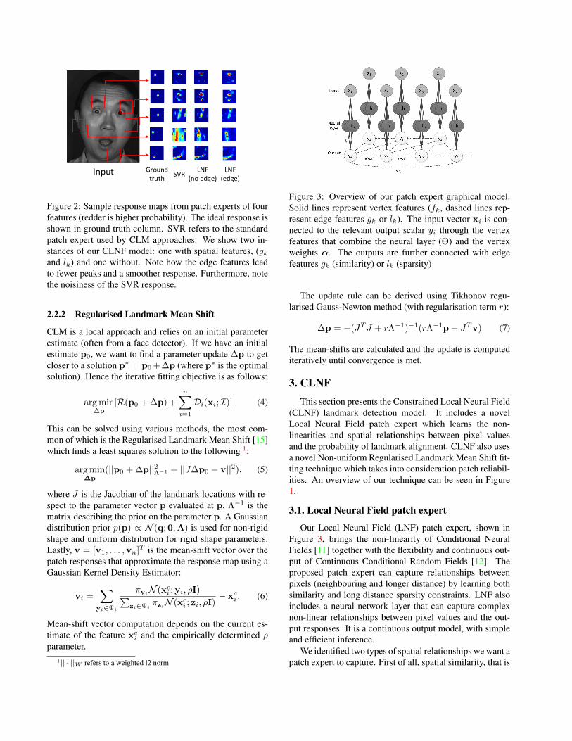
There have been a number of different methods proposedas patch experts: various SVR models and logistic regres-sors, or even simple template matching techniques. Themost popular expert by far is the linear Support Vector Re-gressor in combination with a logistic regressor [3, 15, 20].Linear SVRs are used, because of their computational sim-plicity, and potential for efficient implementation on imagesusing convolution [20]. Some sample response maps frompatch experts can be seen in Figure 2.

Input SVRLNF

(no edge)Ground

truthLNF

(edge)

Figure 2: Sample response maps from patch experts of fourfeatures (redder is higher probability). The ideal response isshown in ground truth column. SVR refers to the standardpatch expert used by CLM approaches. We show two in-stances of our CLNF model: one with spatial features, (gkand lk) and one without. Note how the edge features leadto fewer peaks and a smoother response. Furthermore, notethe noisiness of the SVR response.

2.2.2 Regularised Landmark Mean Shift

CLM is a local approach and relies on an initial parameterestimate (often from a face detector). If we have an initialestimate p0, we want to find a parameter update ∆p to getcloser to a solution p∗ = p0 +∆p (where p∗ is the optimalsolution). Hence the iterative fitting objective is as follows:

arg min∆p

[R(p0 + ∆p) +

n∑i=1

Di(xi; I)] (4)

This can be solved using various methods, the most com-mon of which is the Regularised Landmark Mean Shift [15]which finds a least squares solution to the following 1:

arg min∆p

(||p0 + ∆p||2Λ−1 + ||J∆p0 − v||2), (5)

where J is the Jacobian of the landmark locations with re-spect to the parameter vector p evaluated at p, Λ−1 is thematrix describing the prior on the parameter p. A Gaussiandistribution prior p(p) ∝ N (q; 0,Λ) is used for non-rigidshape and uniform distribution for rigid shape parameters.Lastly, v = [v1, . . . ,vn]T is the mean-shift vector over thepatch responses that approximate the response map using aGaussian Kernel Density Estimator:

vi =∑

yi∈Ψi

πyiN (xci ; yi, ρI)∑

zi∈ΨiπziN (xc

i ; zi, ρI)− xc

i . (6)

Mean-shift vector computation depends on the current es-timate of the feature xc

i and the empirically determined ρparameter.

1|| · ||W refers to a weighted l2 norm

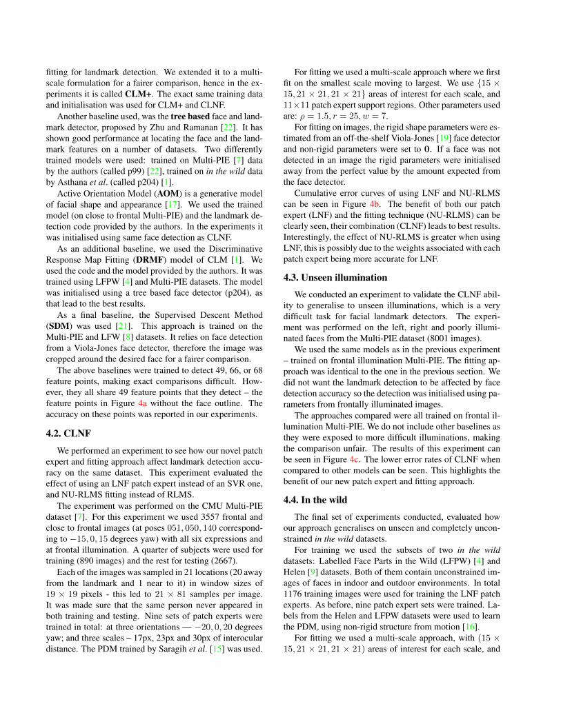
Figure 3: Overview of our patch expert graphical model.Solid lines represent vertex features (fk, dashed lines rep-resent edge features gk or lk). The input vector xi is con-nected to the relevant output scalar yi through the vertexfeatures that combine the neural layer (Θ) and the vertexweights α. The outputs are further connected with edgefeatures gk (similarity) or lk (sparsity)

The update rule can be derived using Tikhonov regu-larised Gauss-Newton method (with regularisation term r):

∆p = −(JTJ + rΛ−1)−1(rΛ−1p− JTv) (7)

The mean-shifts are calculated and the update is computediteratively until convergence is met.

3. CLNFThis section presents the Constrained Local Neural Field

(CLNF) landmark detection model. It includes a novelLocal Neural Field patch expert which learns the non-linearities and spatial relationships between pixel valuesand the probability of landmark alignment. CLNF also usesa novel Non-uniform Regularised Landmark Mean Shift fit-ting technique which takes into consideration patch reliabil-ities. An overview of our technique can be seen in Figure1.

3.1. Local Neural Field patch expert

Our Local Neural Field (LNF) patch expert, shown inFigure 3, brings the non-linearity of Conditional NeuralFields [11] together with the flexibility and continuous out-put of Continuous Conditional Random Fields [12]. Theproposed patch expert can capture relationships betweenpixels (neighbouring and longer distance) by learning bothsimilarity and long distance sparsity constraints. LNF alsoincludes a neural network layer that can capture complexnon-linear relationships between pixel values and the out-put responses. It is a continuous output model, with simpleand efficient inference.

We identified two types of spatial relationships we want apatch expert to capture. First of all, spatial similarity, that is

pixels nearby should have similar alignment probabilities.Secondly, in the whole area the patch expert is evaluated,only one peak should be present. We want to enforce somesparsity in the response.

We visually show the advantages of modelling spatial de-pendencies and input non-linearities in Figure 2, that showspatch responses maps from SVR patch experts [20], ourLNF patch expert without spatial constraints, and our fullLNF patch expert with similarity and sparsity constraints.Note how our patch expert response has fewer peaks and issmoother than the one without edge features, and both ofthem are more accurate than the SVR patch expert. Thesespatial constraints are designed to improve the patch re-sponse convexity, leading to more accurate fitting.

3.1.1 Model definition

LNF is an undirected graphical model that can model theconditional probability of a continuous valued vector y (theprobability that a patch is aligned) depending on continu-ous x (the pixel intensity values in the support region). Agraphical illustration of our model can be seen in Figure 3.

In our discussion we will use the following notation:X = {x1,x2, . . . ,xn} is a set of observed input variables,y = {y1, y2, . . . , yn} is a set of output variables that wewish to predict, xi ∈ Rm represents vectorised pixel inten-sities in patch expert support region (e.g. m = 121 for an11 × 11 support region), yi ∈ R is a scalar prediction atlocation i.

Our model for a particular set of observations is a condi-tional probability distribution with the probability density:

P (y|X) =exp(Ψ)∫∞

−∞ exp(Ψ)dy(8)

Above∫∞−∞ exp(Ψ)dy is the normalisation (partition) func-

tion which makes the probability distribution a valid one (bymaking it sum to 1). The following section describes the po-tential function used by our LNF patch expert.

3.1.2 Potential functions

Our potential function is defined as:

Ψ =∑

i

∑K1k=1 αkfk(yi,X,θk)+∑

i,j

∑K2k=1 βkgk(yi, yj)+∑

i,j

∑K3k=1 γklk(yi, yj)

, (9)

where model parameters α = {α1, α2, . . . αK1}, Θ ={θ1,θ2, . . .θK1}, and β = {β1, β2, . . . βK2}, γ ={γ1, γ2, . . . γK3} are learned and used for inference duringtesting. We define three types of potentials in our model,vertex features fk, and edge features gk, and lk:

fk(yi,X,θk) = −(yi − h(θk,xi))2, (10)

h(θ,x) =1

1 + e−θTx, (11)

gk(yi, yj) = −1

2S

(gk)i,j (yi − yj)2, (12)

lk(yi, yj) = −1

2S

(lk)i,j (yi + yj)

2. (13)

Vertex features fk represent the mapping from the input xi

to output yi through a one layer neural network and θk is theweight vector for a particular neuron k. Θ can be thought ofas a set of convolution kernels that are applied to an area ofinterest. The corresponding αk for vertex feature fk repre-sents the reliability of the kth neuron (convolution kernel).

Edge features gk represent the similarities between ob-servations yi and yj . In our LNF patch expert gk enforcessmoothness on connected nodes. This is also affected bythe neighbourhood measure S(gk), which allows us to con-trol where the smoothness is to be enforced. For our patchexpert we define S(g1) to return 1 (otherwise return 0) onlywhen the two nodes i and j are direct (horizontal/vertical)neighbours in a grid. We also define S(g2) to return 1 (oth-erwise 0) when i and j are diagonal neighbours in a grid.

Edge features lk represent the sparsity constraint be-tween observations yi and yj . For example the model ispenalised if both yi and yj are high, but is not penalised ifboth of them are zero. This has a slightly unwanted conse-quence of penalising just yi or yj being high, but the penaltyfor both of them being high is much bigger. This is con-trolled by the neighbourhood measure S(lk) that allows usto define regions where sparsity should be enforced. Weempirically defined the neighbourhood region S(l) to return1 only when two nodes i and j are between 4 and 6 edgesapart (where edges are counted from the grid layout of ourLNF patch expert).

3.1.3 Learning and Inference

In this section we describe how to estimate the parameters{α,β,γ,Θ}. It is important to note that all of the parame-ters are optimised jointly.

We are given training data {x(q),y(q)}Mq=1 ofM patches,

where each x(q) = {x(q)1 ,x

(q)2 , . . . ,x

(q)n } is a sequence of

inputs (pixel values in the area of interest) and each y(q) =

{y(q)1 , y

(q)2 , . . . , y

(q)n } is a sequence of real valued outputs

(expected response maps).In learning we want to pick the α, β, γ and Θ values

that maximise the conditional log-likelihood of LNF on thetraining sequences:

L(α,β,γ,Θ) =

M∑q=1

logP (y(q)|x(q)) (14)

(α, β, γ, Θ) = arg maxα,β,γ,Θ

(L(α,β,γ,Θ)) (15)

It helps with the derivation of the partial derivatives ofEquation 14 and with explanation of inference to convert theEquation 8 into multivariate Gaussian form (see Baltrusaitiset al. [2] for a similar derivation):

P (y|X) =1

(2π)n2 |Σ| 12

exp(−1

2(y − µ)T Σ−1(y − µ)),

(16)Σ−1 = 2(A+B + C) (17)

The diagonal matrix A represents the contribution of αterms (vertex features) to the covariance matrix, and thesymmetricB and C represent the contribution of the β, andγ terms (edge features).

Ai,j =

K1∑k=1

αk, i = j

0, i 6= j

(18)

Bi,j =

(

K2∑k=1

βk

n∑r=1

S(gk)i,r )− (

K2∑k=1

βkS(gk)i,j ), i = j

−K2∑k=1

βkS(gk)i,j , i 6= j

(19)

Ci,j =

(

K2∑k=1

γk

n∑r=1

S(lk)i,r ) + (

K2∑k=1

γkS(lk)i,j ), i = j

K2∑k=1

γkS(lk)i,j , i 6= j

(20)It is useful to define a vector d, that describes the linearterms in the distribution, and µ which is the mean value ofthe Gaussian form of the CCNF distribution:

d = 2αTh(ΘX). (21)

µ = Σd. (22)

Above X is a matrix where the ith column is xi, Θ isthe concatenated neural network weights and h(M), is anelement-wise application of sigmoid (activation function)on each element of M , and thus h(ΘX) represents the re-sponse of each of the gates (neural layers) at each xi.

Intuitively d is the contribution from the the vertex fea-tures. These are the terms that contribute directly from inputfeatures x towards y. Σ on the other hand, controls the in-fluence of the edge features on the output. Finally, µ is theexpected value of the distribution, hence it is the value of ythat maximises P (y|x).

In order to guarantee that our partition function is inte-grable, we constrain αk > 0 and βk > 0, γk > 0 [12],while Θ is unconstrained.

The log-likelihood can be maximised using constrainedBFGS. We use the standard Matlab implementation of the

algorithm. In order to make the optimisation more accurateand faster we used the partial derivatives of the logP (y|X).

To train our LNF patch expert, we need to define theoutput variables yi. Given an image with a true landmarkat z = (u, v)T we can model the probability of it beingaligned at zi as yi = N (zi; z, σ) (we experimentally foundthat best results are achieved with σ = 1). We can thensample the image at various locations to get training sam-ples. An example of such synthetic response maps can beseen in Figure 2, in the ground truth column.

3.2. Non-uniform RLMS

A problem facing CLM fitting is that each of the patchexperts is equally trusted, but this should clearly not be thecase. This can be seen in Figures 1 and 2, where the re-sponse maps of certain features are noisier. RLMS does nottake this into consideration. To tackle this issue, we proposeminimising the following objective function:

arg min∆p

(||p + ∆p||2Λ−1 + ||J∆p− v||2W . (23)

The diagonal weight matrix W allows for weighting ofmean-shift vectors. Non-linear least squares with TikhonovRegularisation leads to the following update rule:

∆p = −(JTWJ + rΛ−1)(rΛ−1p− JTWv). (24)

Note that, if we use a non-informative identity W = I , theabove collapses to the regular RLMS update rule.

To construct W , we compute the correlation scores ofeach patch expert on the holdout fold of training data. Thisleads toW = w·diag(c1; . . . ; cn; c1; . . . cn), where ci is thecorrelation coefficient of the ith patch expert on the holdouttest fold and w is determined experimentally. The ith andi + nth elements on the diagonal represent the confidenceof the ith patch expert. Patch expert reliability matrix Wis computed separately for each scale and view. This is asimple but effective way to estimate the error expected froma particular patch. Example reliabilities are displayed inFigure 4a.

4. ExperimentsWe conducted a number of experiments to validate the

benefits of the proposed CLNF model. First, an experi-ment was performed to confirm the benefit of both the LNFpatch experts and the NU-RLMS approach to model fitting.The second experiment explored how well the CLNF modelgeneralises to unseen illumination. The final set of exper-iments evaluated how well our approach generalises out ofdatabase and in the wild.

4.1. Baselines

As the first baseline we used the CLM model proposedby Saragih et al. [15]. It uses SVR patch experts and RLMS

fitting for landmark detection. We extended it to a multi-scale formulation for a fairer comparison, hence in the ex-periments it is called CLM+. The exact same training dataand initialisation was used for CLM+ and CLNF.

Another baseline used, was the tree based face and land-mark detector, proposed by Zhu and Ramanan [22]. It hasshown good performance at locating the face and the land-mark features on a number of datasets. Two differentlytrained models were used: trained on Multi-PIE [7] databy the authors (called p99) [22], trained on in the wild databy Asthana et al. (called p204) [1].

Active Orientation Model (AOM) is a generative modelof facial shape and appearance [17]. We used the trainedmodel (on close to frontal Multi-PIE) and the landmark de-tection code provided by the authors. In the experiments itwas initialised using same face detection as CLNF.

As an additional baseline, we used the DiscriminativeResponse Map Fitting (DRMF) model of CLM [1]. Weused the code and the model provided by the authors. It wastrained using LFPW [4] and Multi-PIE datasets. The modelwas initialised using a tree based face detector (p204), asthat lead to the best results.

As a final baseline, the Supervised Descent Method(SDM) was used [21]. This approach is trained on theMulti-PIE and LFW [8] datasets. It relies on face detectionfrom a Viola-Jones face detector, therefore the image wascropped around the desired face for a fairer comparison.

The above baselines were trained to detect 49, 66, or 68feature points, making exact comparisons difficult. How-ever, they all share 49 feature points that they detect – thefeature points in Figure 4a without the face outline. Theaccuracy on these points was reported in our experiments.

4.2. CLNF

We performed an experiment to see how our novel patchexpert and fitting approach affect landmark detection accu-racy on the same dataset. This experiment evaluated theeffect of using an LNF patch expert instead of an SVR one,and NU-RLMS fitting instead of RLMS.

The experiment was performed on the CMU Multi-PIEdataset [7]. For this experiment we used 3557 frontal andclose to frontal images (at poses 051, 050, 140 correspond-ing to −15, 0, 15 degrees yaw) with all six expressions andat frontal illumination. A quarter of subjects were used fortraining (890 images) and the rest for testing (2667).

Each of the images was sampled in 21 locations (20 awayfrom the landmark and 1 near to it) in window sizes of19 × 19 pixels - this led to 21 × 81 samples per image.It was made sure that the same person never appeared inboth training and testing. Nine sets of patch experts weretrained in total: at three orientations — −20, 0, 20 degreesyaw; and three scales – 17px, 23px and 30px of interoculardistance. The PDM trained by Saragih et al. [15] was used.

For fitting we used a multi-scale approach where we firstfit on the smallest scale moving to largest. We use {15 ×15, 21 × 21, 21 × 21} areas of interest for each scale, and11×11 patch expert support regions. Other parameters usedare: ρ = 1.5, r = 25, w = 7.

For fitting on images, the rigid shape parameters were es-timated from an off-the-shelf Viola-Jones [19] face detectorand non-rigid parameters were set to 0. If a face was notdetected in an image the rigid parameters were initialisedaway from the perfect value by the amount expected fromthe face detector.

Cumulative error curves of using LNF and NU-RLMScan be seen in Figure 4b. The benefit of both our patchexpert (LNF) and the fitting technique (NU-RLMS) can beclearly seen, their combination (CLNF) leads to best results.Interestingly, the effect of NU-RLMS is greater when usingLNF, this is possibly due to the weights associated with eachpatch expert being more accurate for LNF.

4.3. Unseen illumination

We conducted an experiment to validate the CLNF abil-ity to generalise to unseen illuminations, which is a verydifficult task for facial landmark detectors. The experi-ment was performed on the left, right and poorly illumi-nated faces from the Multi-PIE dataset (8001 images).

We used the same models as in the previous experiment– trained on frontal illumination Multi-PIE. The fitting ap-proach was identical to the one in the previous section. Wedid not want the landmark detection to be affected by facedetection accuracy so the detection was initialised using pa-rameters from frontally illuminated images.

The approaches compared were all trained on frontal il-lumination Multi-PIE. We do not include other baselines asthey were exposed to more difficult illuminations, makingthe comparison unfair. The results of this experiment canbe seen in Figure 4c. The lower error rates of CLNF whencompared to other models can be seen. This highlights thebenefit of our new patch expert and fitting approach.

4.4. In the wild

The final set of experiments conducted, evaluated howour approach generalises on unseen and completely uncon-strained in the wild datasets.

For training we used the subsets of two in the wilddatasets: Labelled Face Parts in the Wild (LFPW) [4] andHelen [9] datasets. Both of them contain unconstrained im-ages of faces in indoor and outdoor environments. In total1176 training images were used for training the LNF patchexperts. As before, nine patch expert sets were trained. La-bels from the Helen and LFPW datasets were used to learnthe PDM, using non-rigid structure from motion [16].

For fitting we used a multi-scale approach, with (15 ×15, 21 × 21, 21 × 21) areas of interest for each scale, and

(a) Patch reliabilities

0.02 0.0275 0.035 0.0425 0.050

0.2

0.4

0.6

0.8

0.9

Eye distance normalised shape RMS error

Pro

port

ion

of im

ages

SVR + RLMS (CLM+)SVR + NU−RLMSLNF + RLMSLNF + NU−RLMS (CLNF)

(b) Fitting on Multi-PIE

0.01 0.03 0.05 0.07 0.09 0.11 0.13 0.150

0.2

0.4

0.6

0.8

1

Eye distance normalised shape RMS error

Pro

port

ion

of im

ages

CLNFCLM+Tree based (p99)AOM

(c) Fitting across illumination

Figure 4: a) The reliabilities of CLNF patch experts, smaller circles represent more reliability (less variance). b) Fitting onthe Multi-PIE dataset, observe the performance boost from both the LNF patch expert and the NU-RLMS fitting method.Their combination (CLNF) leads to the lowest error, since NU-RLMS performs even better on more reliable response maps.c) Fitting on the unseen illumination Multi-PIE subset. Note the good generalisability of CLNF.

11×11 patch expert support regions. Other parameters usedare: ρ = 2.0, r = 25, w = 5.

In order to evaluate the ability of CLNF to generalise onunseen datasets we evaluated our approach on the datasetslabelled for the 300 Faces in-the-Wild Challenge [14]. Fortesting we used three datasets: Annotated Faces in the Wild[22], IBUG [18] and 300 Faces in-the-Wild Challenge (300-W) [18] datasets. The IBUG, AFW, and 300-W datasetscontains 135, 337, and 600 images respectively.

To initialise model fitting, we used the bounding boxesprovided by the 300 Faces in-the-Wild Challenge [18] thatwere initialised using the tree based face detector [22]. Inorder to deal with pose variation the model was initialised at5 orientations – (0, 0, 0), (0,±30, 0), (0, 0,±30) degrees ofroll, pitch and yaw. The final model with the lowest align-ment error (Equation 4) was chosen as the correct one. Thismakes the approach five times slower, but more robust.

Note that we were unable to use bounding box initialisa-tions for the SDM method, and they were unnecessary fortree based methods.

The results of this experiment can be seen in Figure 5.Our approach can be seen outperforming all of the otherbaselines tested. This confirms the benefits of CLNF andits ability to generalise well to unseen data. Some exam-ples of landmark detections can be seen in Figure 6. CLNFgap between CLNF and CLM+ is much greater on in thewild images than on the constrained ones. Furthermore,note the huge discrepancy between CLNF and the AAMbaseline provided by the authors [10]. This illustrates thegreater generalisability of our proposed model over otherapproaches.

5. ConclusionsWe have presented a Constrained Local Neural Field

model for facial landmark detection and tracking. The twomain novelties of our approach show an improvement in

landmark detection accuracy over state-of-art approaches.Our LNF patch expert exploits spatial relationships be-tween patch response values, and learns non-linear rela-tionships between pixel values and patch responses. OurNon-uniform Regularised Landmark Mean-Shift optimisa-tion technique, allows us to take into account the reliabil-ities of each patch expert leading to better accuracy. Wehave demonstrated the benefit of our approach on a numberof publicly available datasets.

CLNF is also a fast approach: a Matlab implementationcan process 2 images per second on in the wild data, and10 images per second on Multi-PIE data, on a 3.5GHz dualcore Intel i7 machine. Lastly, all of the code and testingscripts to recreate the results will be made publicly avail-able.

AcknowledgementsWe acknowledge funding support from Thales Research

and Technology (UK) and from the European Community’sSeventh Framework Programme (FP7/2007- 2013) undergrant agreement 289021 (ASC-Inclusion). This material ispartially supported by the U.S. Army Research, Develop-ment, and Engineering Command (RDECOM). The con-tent does not necessarily reflect the position or the policyof the Government, and no official endorsement should beinferred.

References[1] A. Asthana, S. Zafeiriou, S. Cheng, and M. Pantic. Robust

discriminative response map fitting with constrained localmodels. In CVPR, 2013.

[2] T. Baltrusaitis, N. Banda, and P. Robinson. Dimensional af-fect recognition using continuous conditional random fields.In FG, 2013.

[3] T. Baltrusaitis, P. Robinson, and L.-P. Morency. 3D Con-strained Local Model for Rigid and Non-Rigid Facial Track-ing. In CVPR, 2012.

0 0.05 0.1 0.150

0.2

0.4

0.6

0.8

1

Eye distance normalised shape RMS error

Pro

port

ion

of im

ages

CLNF (ours)SDMTree based (p204)CLM+DRMF

(a) AFW

0 0.05 0.1 0.15 0.20

0.2

0.4

0.6

0.8

1

Eye distance normalised shape RMS error

Pro

port

ion

of im

ages

CLNF (ours)SDMTree based (p204)CLM+DRMF

(b) IBUG

0 0.05 0.1 0.150

0.2

0.4

0.6

0.8

1

Size normalised shape RMS error

Pro

port

ion

of im

ages

CLNF (68)CLNF (51)AAM (51)AAM (68)

(c) 300W

Figure 5: Fitting on the wild datasets using our CLNF approach and other state-of-the-art methods. All of the methods havebeen trained on in the wild data from different than test datasets. The benefit of CLNF in generalising on unseen data is clear.Furthermore, CLNF remains consistently accurate across all three test sets. a) Testing on the AFW dataset. b) Testing on theIBUG dataset. c) Testing on the challenge dataset [18], error rates using just internal and all of the points are displayed.

Figure 6: Examples of landmark detections in the wild using CLNF. Top row is from IBUG dataset, bottom row from AFW.Notice the generalisability across pose, illumination, and expression. The model can also deal with occlusions.

[4] P. N. Belhumeur, D. W. Jacobs, D. J. Kriegman, and N. Ku-mar. Localizing parts of faces using a consensus of exem-plars. In CVPR, 2011.

[5] D. Cristinacce and T. Cootes. Feature detection and trackingwith constrained local models. In BMVC, 2006.

[6] N. Dalal and B. Triggs. Histograms of oriented gradients forhuman detection. In CVPR, pages 886–893, 2005.

[7] R. Gross, I. Matthews, J. Cohn, T. Kanade, and S. Baker.Multi-pie. IVC, 28(5):807 – 813, 2010.

[8] G. B. Huang, M. Ramesh, T. Berg, and E. Learned-Miller.Labeled Faces in the Wild: A Database for Studying FaceRecognition in Unconstrained Environments. 2007.

[9] V. Le, J. Brandt, Z. Lin, L. Bourdev, and T. S. Huang. Inter-active facial feature localization. In ECCV, 2012.

[10] I. Matthews and S. Baker. Active appearance models revis-ited. IJCV, 60(2):135–164, 2004.

[11] J. Peng, L. Bo, and J. Xu. Conditional neural fields. NIPS,2009.

[12] T. Qin, T.-Y. Liu, X.-D. Zhang, D.-S. Wang, and H. Li.Global ranking using continuous conditional random fields.In NIPS, 2008.

[13] P. Robinson and R. el Kaliouby. Computation of emo-tions in man and machines. Philosophical Transactions B,364(1535):3441–3447, 2009.

[14] C. Sagonas, G. Tzimiropoulos, S. Zafeiriou, and M. Pantic.A semi-automatic methodology for facial landmark annota-tion. In Workshop on Analysis and Modeling of Faces andGestures, 2013.

[15] J. Saragih, S. Lucey, and J. Cohn. Deformable Model Fittingby Regularized Landmark Mean-Shift. IJCV, 2011.

[16] L. Torresani, A. Hertzmann, and C. Bregler. Nonrigidstructure-from-motion: estimating shape and motion with hi-erarchical priors. TPAMI, 30(5):878–892, May 2008.

[17] G. Tzimiropoulos, J. Alabort-i Medina, S. Zafeiriou, andM. Pantic. Generic Active Appearance Models Revisited.In ACCV, pages 650–663, 2012.

[18] G. Tzimiropoulos, S. Zafeiriou, and M. Pantic. 300 facesin-the-wild challenge, 2013.

[19] P. Viola and M. J. Jones. Robust real-time face detection.IJCV, 57(2):137–154, 2004.

[20] Y. Wang, S. Lucey, and J. Cohn. Enforcing convexity for im-proved alignment with constrained local models. In CVPR,2008.

[21] X. Xiong and F. De la Torre. Supervised descent method andits applications to face alignment. In CVPR, 2013.

[22] X. Zhu and D. Ramanan. Face detection, pose estimation,and landmark localization in the wild. CVPR, 2012.