Design of Robust PID Controllers with Constrained Control ... · PDF fileDesign of Robust PID...
122
Design of Robust PID Controllers with Constrained Control Signal Activity Olof Garpinger Department of Automatic Control Lund University Lund, March 2009
Transcript of Design of Robust PID Controllers with Constrained Control ... · PDF fileDesign of Robust PID...

Design of Robust PIDControllers with Constrained
Control Signal Activity
Olof Garpinger
Department of Automatic Control
Lund University
Lund, March 2009

Department of Automatic ControlLund UniversityBox 118SE-221 00 LUNDSweden
ISSN 0280–5316ISRN LUTFD2/TFRT--3245--SE
c© 2009 by Olof Garpinger. All rights reserved.Printed in Sweden,Lund University, Lund 2009

Abstract
This thesis presents a new method for design of PI and PID controllerswith the level of control signal activity taken into consideration. Themain reason why the D-part is often disabled in industrial control loopsis because it leads to control signal sensitivity of measurement noise.A frequently varying control signal with too high amplitude will verylikely lead to actuator wear and tear. For this reason it is extremelyimportant for any PID design method to take this into account.The proposed controllers are derived using a newly developed de-
sign software that solves an IAE minimization problem with respectto H∞ robustness constraints on the sensitivity- and complementarysensitivity function. The software is shown to be fast, easy to use androbust in giving well-performing controllers.By extracting measurement noise from the process value of a real
plant, one can estimate its effect on the control signal variance. Thetime constant of the low-pass filter, through which measurements arefed, is varied to design controllers with constrained control signal ac-tivity. By comparing control signal variance and IAE, the user is alsoable to weigh actuator wear to estimated performance.The proposed PID design method has shown to give very promising
results both on simulated examples and real plants such as a recircu-lation flow process.Optimal Youla parametrized controllers are used both as a quality
check of the designed PI and PID controllers and as a tool for de-termining when these are valid choices compared to more advancedcontrollers.
3


Acknowledgments
After three and a half years at the Department of Automatic Control inLund there are several people that I would like to thank. The personthat, without doubt, has my greatest appreciation is my supervisor,Tore Hägglund. You have always been available, no matter what I havewanted to discuss. I do not think there has been one single meetingwith you, after which I have not walked out more motivated than whenI walked in. You will always be a role model to me Tore, both as aresearcher and as a person.I am lucky to have many gifted colleagues and I owe some of them a
lot for helping me come up with my ideas. Karl-Johan Åström for givingme the idea to rewrite Pontus Nordfeldt’s original PID design softwareand for making me take a closer look at control signal sensitivity due tomeasurement noise. Andreas Wernrud for introducing me to the ideasof optimal Youla parametrized controllers and for providing me withthe software that carries it out. Per-Ola Larsson has also had a lot ofinfluence on my ideas after numerous discussions in "Fabriksrummet".I’d also like to thank Per-Ola and Tore for all time they have spentreading this thesis and coming with good comments.I want to give my warmest thanks to Rasmus Olsson (pidab ab) and
Erik Falkeman (Akzo Nobel Functional Chemicals AB) for making itpossible for me to try out my ideas on an industrial plant. Without thishelp, my thesis would not have felt as complete.The Department of Automatic Control is also very lucky to have
plenty of people that makes work easier for the rest of us. Manythanks to our secretaries Eva Schildt, Britt-Marie Mårtensson, Ag-
5

Acknowledgments
neta Tuszynski and Eva Westin for helping and lifting the mood onall of us. Thanks to Leif Andersson and Anders Blomdell for all helpregarding computers and for keeping them running smoothly. Thanksto Rolf Braun for making it possible to run my lab tests smoothly.Besides this, I would also like to thank those brave persons that eat
lunch in the city close to every week. Especially Anton and Toivo whohave always appreciated the combination of fresh air, good food andexercise. It is also in place to thank my parents for always believing inand supporting me over the years, no matter what I have wanted todo. You should know that I am very grateful for this.
6

Contents
1. Introduction . . . . . . . . . . . . . . . . . . . . . . . . . . 91.1 Background . . . . . . . . . . . . . . . . . . . . . . . . 91.2 What are reasonable control goals for industry? . . . 101.3 Is there a need for a new PID design method? . . . . 111.4 Outline . . . . . . . . . . . . . . . . . . . . . . . . . . . 12
2. Design Specifications . . . . . . . . . . . . . . . . . . . . . 142.1 Design criterias . . . . . . . . . . . . . . . . . . . . . . 142.2 Youla parametrized controllers . . . . . . . . . . . . . 192.3 System description for Youla optimization . . . . . . 21
3. Sources of Inspiration and Related Design Methods 233.1 Closely related PID design methods . . . . . . . . . . 233.2 More distantly related methods and sources of inspi-
ration . . . . . . . . . . . . . . . . . . . . . . . . . . . 28
4. A Software Tool for Robust PID Design . . . . . . . . 304.1 Algorithm overview . . . . . . . . . . . . . . . . . . . 304.2 Algorithm details . . . . . . . . . . . . . . . . . . . . . 324.3 PI control . . . . . . . . . . . . . . . . . . . . . . . . . 454.4 Examples . . . . . . . . . . . . . . . . . . . . . . . . . 47
5. Adjustable Control Signal Noise Reduction . . . . . . 525.1 Principle . . . . . . . . . . . . . . . . . . . . . . . . . . 535.2 Challenges with the use of a variance constraint . . 615.3 Suggested procedure for design of PID controllers on
real processes . . . . . . . . . . . . . . . . . . . . . . . 67
7

Contents
5.4 Examples . . . . . . . . . . . . . . . . . . . . . . . . . 67
6. Industrial Example . . . . . . . . . . . . . . . . . . . . . . 876.1 Background . . . . . . . . . . . . . . . . . . . . . . . . 876.2 Initial tests . . . . . . . . . . . . . . . . . . . . . . . . 886.3 Modeling the process . . . . . . . . . . . . . . . . . . . 896.4 Noise data collection . . . . . . . . . . . . . . . . . . . 906.5 Controller designs . . . . . . . . . . . . . . . . . . . . 906.6 Comparison with Youla controllers . . . . . . . . . . . 936.7 Results and conclusions . . . . . . . . . . . . . . . . . 95
7. When are PI and PID Controllers Valid Choices? . . 1017.1 Sub-batch 1 – First order systems with time delay . 1027.2 Sub-batch 2 – Second order systems with time delay 1057.3 Sub-batch 9 – Systems with complex poles . . . . . . 1097.4 Summary . . . . . . . . . . . . . . . . . . . . . . . . . 111
8. Conclusions and Future Work . . . . . . . . . . . . . . . 1148.1 Conclusions . . . . . . . . . . . . . . . . . . . . . . . . 1148.2 Future work . . . . . . . . . . . . . . . . . . . . . . . . 116
9. Bibliography . . . . . . . . . . . . . . . . . . . . . . . . . . 117
8

1
Introduction
This chapter will present some of the main goals of the PID designmethod proposed in this thesis. It will be followed by a motivationfor developing new methods for PID design when there are alreadyseveral in use giving satisfying results. The chapter will be concludedwith an outline of the thesis, summarizing the content of the respectivechapters.
1.1 Background
Many industrial processes have rather simple dynamics and they are,therefore, often modeled using straightforward methods like step re-sponse tests. This will typically lead to models of the form
P(s) = Kp
1+ sT e−sL, (1.1)
called First Order systems with Time Delay or just FOTD systems.One way of characterizing these processes is by the normalized timedelay
τ = L
L + T . (1.2)
When τ & 0, the process is called lag dominant, while a process withτ . 1 is referred to as delay dominant. τ is used extensively in, for
9
Chapter 1. Introduction
example, [Åström and Hägglund, 2005]. While τ is introduced for FOTDsystems, it is a measure used for a much broader variety of systems(through FOTD approximation). For this reason, τ will be frequentlyused in this thesis as well.The PI controller is, by far, the most common controller in industry
today. Although a PI controller may often be sufficient, the main reasonfor the rare use of the D-part is due to measurement noise throughputto the control signal and the complexity of choosing yet another param-eter. While PI and PID controllers are considered to give rather simplecontrol laws, there are still a lot of poorly tuned controllers in industry.Two of the main reasons being lack of knowledge and time among theoperators. As a consequence, many PID controllers have their param-eters set to default values. So, it is important for any controller designmethod to be fast, simple and robust. If not, there is little chance itwill be used.
1.2 What are reasonable control goals for industry?
In order to derive a successful controller design tool, no matter thecontroller structure, it is important to set reasonable demands on theclosed loop system. Here follows a brief list of closed loop characteristicsthat the proposed design tool was built upon:
• Fast suppression of load disturbances
According to [Åström and Hägglund, 2005], the most important dutyof the industrial controller is to suppress low frequency changes on theprocess value. Too high variations in the process value could typicallylead to lower product quality.
• Modeling errors and process alteration not leading to instability
As stated already, the dominating method for derivation of an indus-trial process model is by running a step response test in open loop. Thiswill likely result in an FOTD model like (1.1), no matter if the trueprocess dynamics are much more complex or not. Even if the model isgood to start with, it could very well be that the plant changes slowly
10

1.3 Is there a need for a new PID design method?
over time. In other words, it is important that the closed loop systemis robust to such errors and variations.
• Actuator wear and tear should be low
For anyone that wants to design a PID controller where the D-part isactive, it is extremely important that the control signal activity doesnot become too high. In this thesis, it will be assumed that high ampli-tude and frequency of the control signal are the major villains when itcomes to cause actuator wear and tear. In [Buckbee, 2002], the relationbetween high expenses of valve maintenance and controller tuning arein focus. Buckbee emphasizes the commercial value of proper tuningin order to keep the control signal activity low.
1.3 Is there a need for a new PID design method?
It has already been mentioned that many industrial control loops arepoorly tuned, often without use of any systematic design method. Thereare, however, several design methods that are used rather frequentlyin industry. The possibly most common of these is the lambda tuningmethod, which will be described in detail in the next chapter. Anothercommon method is auto-tuning which determines a controller through,for example, relay and/or step response experiments on the process.These kinds of design methods are often incorporated in commercialsoftware programs.While many control loops can be controlled sufficiently well with
these methods, they often lack guarantees that all three criterias inSection 1.2 are addressed. It could, for instance, be that a PI designgives a robust closed loop system with low control signal activity, butrather bad performance. A PID controller may then be a better op-tion for fulfilling all demands on the system. The PID design methodproposed in this thesis will take all three criterias into account simul-taneously and should thus more likely be giving good control. Anotherfundamental aspect of the new design method is to choose either PIor PID control structure depending on which is the most suitable forthe given process. For example, there is no reason to design a moreadvanced controller if a PI controller is just as good.
11

Chapter 1. Introduction
Furthermore, the proposed PID design method is software based,solving an optimization problem off-line (see [Garpinger and Hägglund,2008]). Many other design methods are formula based, with their originfrom some advanced optimization, like [Kristiansson and Lennartson,2006] and [Hägglund and Åström, 2004]. But, if it is possible to solvethe optimization directly on a computer, should it then not be betterthan using a generalized formula? It was shown in [Garpinger andHägglund, 2008] that the proposed software program has good poten-tial of being both a source for PID knowledge and a tool for furtherresearch. Such a tool can, in other words, be beneficial to people inindustry in need of more PID education, at the same time as it is usedby advanced researchers.In order to get a quality check of the PI and PID controllers, de-
rived by the proposed design method, Youla parametrized controllershave been used. A Youla optimization tool was used to derive nearlyoptimal linear controllers with the same criterias as the PID design.This way, one can see how close the controller designs are to the limitof performance. There will also be an attempt to use Youla controllersfor giving a more general picture of when PI and PID controllers areuseful compared to more advanced controllers.
1.4 Outline
Here follows a brief summary of the different thesis chapters.
Chapter 2
In Chapter 2 follows a presentation of the closed loop system in focus.In conjunction to this, an optimization problem is stated such that thecriterias in Section 1.2 are taken into consideration. The chapter is alsoconcerned with giving an introduction to the way Youla parametrizedcontrollers can be optimized to give good estimates of the best possiblelinear controllers. The optimization problem is finally translated intoa Youla parametrization framework for convex optimization.
Chapter 3
Chapter 3 introduces four other PID design methods, some sources ofinspiration and a few other related methods.
12

1.4 Outline
Chapter 4
Chapter 4 contains a detailed explanation of how the proposed softwaretool for optimization of robust PID controllers works. The Nelder Meadalgorithm is presented together with a motivation of its worth. Thechapter is concluded with several examples, comparing the PI and PIDcontrollers to those derived with the MIGO method (for a descriptionof the MIGO method, see Section 3.1).
Chapter 5
The purpose of Chapter 5 is to describe how the PID design softwarecan be used to constrain the control signal variance due to measure-ment noise. Challenges in connection to e.g. measurement data loggingand variance estimation are also discussed. A suggestion on how toproceed with the method on a real plant is also presented. Several ex-amples will conclude the chapter and show the potential of the method.Optimized Youla controllers will be used to validate the quality of thePI and PID controllers.
Chapter 6
The proposed PID design method has been tried out on an industrialplant. The chapter describes initial tests, modeling of the plant, con-troller design and results when the proposed controllers were run ona recirculation flow process.
Chapter 7
When is it justified to use PI and PID controllers rather than moreadvanced controllers? Chapter 7 will aim at giving at least a hint ofthe answer to this question. The research on this topic is, however,not yet finished, so the discussion will mainly serve as a source ofinspiration. It should, however, still be possible to draw quite a fewinteresting conclusions from the results.
Chapter 8
The very last chapter will summarize the most important conclusionsand present some ideas for future work in the research area.
13

2
Design Specifications
The following chapter will define the closed loop system of interest inthis thesis. Given this, an optimization problem for design of robustPID controllers with adjustable control signal noise reduction will bestated. In addition to this, there will be two sections describing Youlaparametrized controllers and how to rewrite the closed loop system tofit it into this framework.
2.1 Design criterias
The main purpose of proposed PID controller design tool is to workwell for systems common in process industry. The kind of plants en-countered there are often stable, monotone and primarily affected bylow frequency load disturbances. This is also why the regulator prob-lem is considered in this thesis rather than the tracking problem. Agood tracking performance can be achieved using feed-forward designafter the controller have been designed for disturbance rejection, seee.g. [Åström and Hägglund, 2005] for details.In order for the controller design to work well on a real process,
with model P(s), it is important to take all system signals into con-sideration, especially if optimization is used. If not, some signals mayeasily blow out of proportions or the closed loop could become sensitiveto changes in the process. Figure 2.1 shows a block diagram of the sys-tem that the PID (or PI) controller, C(s), is designed for. There are twoexternal signals entering the system, the load disturbance d (mainly
14

2.1 Design criterias
d
ΣΣe u u y
n
y
–1
C(s) P(s)
Figure 2.1 A load disturbance, d, and measurement noise, n, act on the closedloop system with process P(s) and PID controller C(s).
low frequency) and measurement noise n (assumed high frequency).A popular name for the four transfer functions from disturbances tocontrol signal u and measurement signal y is the gang of four. Theseare
(
T(s) P(s)S(s)C(s)S(s) S(s)
)
=
P(s)C(s)1+ P(s)C(s)
P(s)1+ P(s)C(s)
C(s)1+ P(s)C(s)
11+ P(s)C(s)
,
where the top left corner function, T(s), is called the complementarysensitivity function and the function in the bottom right corner, S(s),is named the sensitivity function.The PID controller is assumed to be on parallel form
C(s) = K(
1+ 1sTi
+ sTd)
⋅1
1+ sTf + (sTf )2/2,
with a second order low pass filter on the measurement signal. In casea PI controller is designed instead, it will have the form
C(s) = K(
1+ 1sTi
)
⋅1
1+ sTf.
15

Chapter 2. Design Specifications
Tf is chosen, in both cases, to weigh the degree of measurement noiserejection against closed loop performance. A low value on Tf will gener-ally result in better load disturbance rejection, but may lead to strongnoise amplification in the control signal. Therefore, choosing T f is abalance between getting good performance and keeping the actuatorwear low. A large portion of this thesis will be focused on how to chooseTf in a sensible way. The low-pass filter has been chosen to be of sec-ond order, even though it is common in industry to only have low-passfilter of order one and then often on the derivative part of the con-troller only. The reason for choosing a second order filter is because itguarantees roll-off on all sensitivity functions (The Gang of Four). Itdoes also make sense to filter the P-part of the controller as it couldotherwise lead to considerable noise throughput to the control signal.It should, however, be possible to use a different low-pass filter setupfor the method described in this thesis if desired, but it would requiresome modifications to the software.The objective of the proposed PID design method is to find the PID
controller giving the least Integrated Absolute Error (IAE) value,
IAE =∞∫
0
pe(t)pdt,
when a load disturbance d, modelled as a step, is acting on the closedloop system. The optimization is done under the constraints that theopen loop Nyquist curve is tangent to one or two prespecified circles inthe complex plane, without entering either of them (see Figure 2.2).These two circles will be called the Ms- and Mp-circle (although theywill sometimes be referred to as the M -circles), which sizes and posi-tions are given by
Ms = maxωpS(iω )p, Mp = max
ωpT(iω )p,
hence the names. According to, for example, [Åström and Hägglund,
16

2.1 Design criterias
−4 −3 −2 −1 0 1−2
−1.5
−1
−0.5
0
0.5
1
1.5
2
Real axis
Imag
inar
y ax
is
Figure 2.2 The Ms-circle (dashed), Mp-circle (dash-dotted) and the open loopNyquist curve (solid) when the optimization criterias are fulfilled.
2005] the center points and radius of the two circles are given by:
CMs = −1, RMs =1Ms,
CMp = −M2p
M2p − 1, RMp =
Mp
M2p − 1,
where the center points are denoted with C, the radius with R and theindices refer to the circles.
17

Chapter 2. Design Specifications
The resulting, non-convex, optimization problem can be written as
minK ,Ti,Td∈R+
∞∫
0
pe(t)pdt = IAEload (2.1)
subject to pS(iω )p ≤ Ms, pT(iω )p ≤ Mp, ∀ω ∈R+,pS(iω s)p = Ms and/or pT(iω p)p = Mp
where e(t) is the control error, ω s are frequencies for which the openloop frequency response is tangent to the Ms-circle and vice versa forω p
on the Mp-circle. Either ω s or ω p could be an empty vector, but not atthe same time. Small Ms- and Mp-values result in large circles. In thesoftware, the maximum allowed Ms- and Mp-values can be prespecifiedby the user. The Ms- and Mp- criterias are known to set the closed looprobustness towards process variations, disturbances and nonlinearitiesas described in [Åström and Hägglund, 2005]. Ms = Mp = 1.4 hasbeen chosen as default values in the optimization software, resultingin 41.8○ phase margin and a gain margin of 3.5. Some sources listvalues spanning from 1.2 to 2 giving reasonable robustness. MIGO onthe other hand uses a simplified robustness criterion called the M -circle, defined as the smallest circle that encloses both the Ms- andMp-circle.In Chapter 5, a constraint on the control signal variance, due to
measurement noise, will be added. This constraint is, therefore, set onC(s)S(s) which will be called Sk(s) in the future. When the spectrumof the measurement noise is taken into consideration, Sk(s)N(s) willbe used instead. N(s) is assumed to be the transfer function filter-ing white noise into the current measurement noise. In this thesis avariance constraint on the control signal was selected, such that
qSkq22 =σ 2uσ 2n
≤ Vk,
where σ 2n is the variance of the measurement noise and σ 2u is the vari-ance of the control signal that the noise results in. Vk is the designparameter and Vk = 1 will correspond to u and n having the samevariance.
18

2.2 Youla parametrized controllers
One could argue that the optimization problem lack a warranty fortime delay robustness. Such a constraint will, however, not be used inthis thesis. Main reason being that PI and PID controllers seldom leadto closed loop systems with poor robustness towards time delay vari-ations. The issue will, however, come up when comparing the designsto more advanced Youla controllers in Chapter 5.
2.2 Youla parametrized controllers
Assume that the process, P(s), is both stabilizable and detectable. Amore general way of representing a closed loop system around P(s)is shown in Figure 2.3. The feedback scheme presented in Figure 2.1is just one possible loop among all that can be represented this way.The signals in w are exogenous disturbances acting on the closed loop,such as: measurement noise, load disturbances and reference signals.The exogenous outputs, z, on the other hand represent the closed loopsignals one wants to control. u is simply the control signal, while eare generally measurements entering the controller. P(s) is a moregeneralized representation of the process and will be used here whenderiving, so called, Youla parametrized controllers.
C(s)
u e
w
P(s)z
Figure 2.3 A general representation of a closed loop system. P is the gener-alized process that will be used to find Youla parametrized controllers.
It is known (see for instance [Boyd et al., 1990] and [Wernrud,2008]) to be possible to parametrize all stable control loops to dependaffinely on the transfer function Q, defined as
Q(s) = C(s)1+ P(s)C(s) . (2.2)
19

Chapter 2. Design Specifications
Many known control problems can then be written such that they areclosed loop convex in Q. Some examples of closed loop convex cost func-tions and constraints are:
• l1- and l2-norm costs.
• Time domain envelop constraints on the closed loop.
• Frequency domain upper bound constraints.
• Upper bound on the H2-norm of a closed loop transfer function.
The stability of the controller C(s) can, however, not be guaranteed,nor can its order be constrained. This means that the controller couldend up having very high order and potentially be unstable. The closedloop must still be stable of course.When the closed loop convex optimization problems are solved, it is
commonly done in discrete time. One way of optimizing the controlleris by defining Q as an FIR filter,
Q(z) =NQ−1∑
l=0ql z
−l,
and then have an optimization solver determine the coefficients ql.The controller can then readily be derived from (2.2). C(z) will bean estimate of the best possible linear controller for the optimizationproblem. The order of the FIR filter will determine how close to thelimit of performance one gets.The optimization tool used here for deriving Youla parametrized
controllers is described in [Wernrud, 2008]. The main use of thesecontrollers in this thesis is to show whether or not the PI and PIDcontroller designs can come close to the limit of performance. As statedin [Boyd et al., 1990], this would be a very strong point in favour of asimple controller.For more information on Youla parametrized controllers one can
read any of the sources; [Norman and Boyd, 1989], [Boyd et al., 1990],[Boyd and Barratt, 1991], [Boyd and Barratt, 1992], [Wernrud, 2008].
20

2.3 System description for Youla optimization
2.3 System description for Youla optimization
In order to derive Youla parametrized controllers for the given problem,the process has to be written on the general form shown in Figure 2.3.For this reason, the process P(s) is transformed to state space form
x(t) = Ax(t) + Bu(t) = Ax(t) + B(d(t) + u(t))y(t) = Cx(t).
The exogenous inputs, w, and outputs, z, are defined as
w(t) =(
d(t)n(t)
)
, z(t) =(
y(t)u(t)
)
,
such that the outputs from the general system, P, are
(
z(t)e(t)
)
=
y(t)u(t)e(t)
=
Cx(t)d(t) + u(t)–Cx(t)–n(t)
.
The complete state space form of P, is thus
x(t) = Ax(t) + ( Bw Bu )(
w(t)u(t)
)
= Ax(t) + ( B 0 B )
d(t)n(t)u(t)
(
z(t)e(t)
)
=(
Cz
Cy
)
x(t) +(
Dzw Dzu
Dyw Dyu
)
(
w(t)u(t)
)
=
C
0
–C
x(t) +
0 0 0
1 0 1
0 –1 0
d(t)n(t)u(t)
.
Since P often contains time delays and the Youla optimization softwareneeds a discrete time system, the process model is discretized witha sampling time h, before P is derived. The form of the state spacerealization is, however, not changed by the discretization.
21

Chapter 2. Design Specifications
By block diagram calculations, one can easily derive the closed loopsystem transfer matrix
H =
P
1+ PC –PC
1+ PC1
1+ PC –C
1+ PC
,
which holds all sensitivity functions of interest for the optimizationproblem.When the Youla optimization is run, the order of the Q-filter needs
to be above a certain number (changes depending on the process) inorder for the final controller to hold an integrator.The sampling time selection is especially vital for delay dominant
systems. The sampling interval should be chosen short enough to coverall vital parts of the system dynamics. At the same time it should notbe too small. A sampling interval shorter than the time delay will berepresented in extra states as described in for instance [Åström andWittenmark, 1997]. If the sampling time, h, is a lot smaller than thetime delay, L, the discrete time system will be of very high order, typi-cally leading to very slow optimization and potentially even numericalproblems.
22

3
Sources of Inspiration and
Related Design Methods
In this chapter, four methods for design of PID controllers will be pre-sented. They all have in common that they will be frequently referredto later within this thesis. In addition to these, the chapter will be con-cluded by a brief overview of other related methods and some sourcesof inspiration.
3.1 Closely related PID design methods
There are many PID design methods available today and some of themost famous are collected and analysed in [Åström and Hägglund,2005]. A few of these will briefly be presented in this section as well,together with a newer method developed in [Nordfeldt, 2005].
Lambda tuning
The lambda tuning method which was first introduced in [Dahlin, 1968]has grown to be very commonly used in industry (see e.g. [Olsen andBialkowski, 2002]). The method is built around the idea of pole place-ment in relation to the process time constant.An FOTD model, like (1.1), is first derived through for instance
a step response experiment on the process. The integral time is then
23

Chapter 3. Sources of Inspiration and Related Design Methods
chosen to be Ti = T such that the open loop transfer function becomes
P(s)C(s) = KpKsTe−sL,
in case of a PI controller. Note that the process pole has been canceledby the controller zero. Using a Taylor series approximation of the timedelay will now make it possible set an approximate closed loop systemtime constant, which will be called Tcl. The lambda tuning formulasfor PI parameters thus becomes
K = 1Kp
T
L + Tcl,
Ti = T .
There are PID controller formulas as well, but these are not as com-monly used.As stated in [Åström and Hägglund, 2005], the lambda tuning rules
will give good control under certain circumstances. The cancellation ofthe process pole will, however, give sluggish load disturbance responsesfor lag-dominant processes (τ & 0). The method do have several ad-vantages as well, since it is both a simple and intuitive method to use.It should, however, be pointed out that there are no guarantees ongood performance, robustness or low control signal activity. Take forinstance the PI design for
P(s) = 10.1s+ 1 e
–s
as an example. According to [Åström and Hägglund, 2005], choosingTcl = 3T is normally considered to give good robustness. With thisprocess, however, one would have to choose Tcl ( 16.8T in order to getthe same robustness as the one, by default, given by the proposed PIDdesign software. Also, setting this Tcl will lead to a controller givingvery poor performance. Cases like this can of course be taken care of bypeople with good control knowledge, but it corresponds to unnecessarywork if there are methods giving good controllers right away.
24

3.1 Closely related PID design methods
The MIGO and AMIGO methods
The method used to receive initial controllers in the proposed softwarealgorithm is called AMIGO (see [Hägglund and Åström, 2004]), whichis a tool for robust PID (and PI) synthesis. To understand AMIGO, itis also important to understand the MIGO method (see [Panagopouloset al., 2002]) for PI and PID design.The optimization problem that the MIGO design deals with is very
similar to (2.1). But instead of minimizing over the IAE-value, it usesthe Integrated Error,
IEload =∞∫
0
e(t)dt,
as cost function and the M -circle as robustness constraint, to determinethe PID parameters.The IE cost is proportional to 1/ki = Ti/K , which reduces the prob-
lem to maximizing the ki-gain over the robustness area. Such an op-timization problem is advantageous as it can be solved by known op-timization routines. There are, however, a few drawbacks related tothe use of the IE-value and it can sometimes be an insufficient costfunction. The IE-cost will decrease if the load disturbance responseassumes negative values, which means that oscillating responses maybe preferred. The M -circle criterion will prevent the worst of the os-cillatory responses from occurring, but there are examples when eventhis is not enough. The problem has been avoided in the final MIGO-algorithm by a fix that searches for the the best controller for whichthe cost function has a defined gradient.A drawback with the MIGO method is that it requires quite a bit
of preparational work before it can run.
25

Chapter 3. Sources of Inspiration and Related Design Methods
The AMIGO design is basically a set of formulas yielding K , Ti andTd. These were derived using MIGO on a test batch, which includes134 systems commonly encountered in process industry
P1(s) =e−s
1+ sT ,
T = 0.02,0.05,0.1,0.2,0.3,0.5,0.7,1,1.3,1.5,2, 4, 6,8, 10,20,50,100,200,500,1000
P2(s) =e−s
(1+ sT)2 ,
T = 0.01,0.02,0.05,0.1,0.2,0.3,0.5,0.7,1,1.3,1.5,2, 4, 6,8, 10,20,50,100,200,500
P3(s) =1
(s+ 1)(1+ sT)2 ,
T = 0.005,0.01,0.02,0.05,0.1,0.2,0.5,2,5, 10
P4(s) =1
(s+ 1)n ,
n = 3, 4, 5, 6, 7, 8
P5(s) =1
(1+ s)(1 +α s)(1+α 2s)(1+α 3s) ,
α = 0.1,0.2,0.3,0, 4,0.5,0.6,0.7,0.8,0.9
P6(s) =1
s(1+ sT1)e−sL1 ,
L1 = 0.01,0.02,0.05,0.1,0.2,0.3,0.5,0.7,0.9,1.0, T1 + L1 = 1
P7(s) =1
(1+ sT)(1 + sT1)e−sL1 , T1 + L1 = 1,
T = 1,2, 5, 10 L1 = 0.01,0.02,0.05,0.1,0.3,0.5,0.7,0.9,1.0
P8(s) =1−α s
(s+ 1)3 ,
α = 0.1,0.2,0.3,0.4,0.5,0.6,0.7,0.8,0.9,1.0,1.1
P9(s) =1
(s+ 1)((sT)2 + 1.4sT + 1) ,
T = 0.1,0.2,0.3,0.4,0.5,0.6,0.7,0.8,0.9,1.0.
(3.1)
Secondly, each and every process in the batch was approximated asan FOTD, (1.1). PID-parameter formulas were then derived through
26

3.1 Closely related PID design methods
parameter fittings with respect to normalized time delay, τ , resultingin
K A = 1Kp
(
0.2+ 0.45TL
)
T Ai =0.4L+ 0.8TL + 0.1T L
T Ad =0.5LT0.3L+ T .
The index A denotes the AMIGO parameters. There are also AMIGOformulas for PI control, namely
K A = 0.15Kp
+(
0.35− LT
(L+ T)2)
T
KpL,
T Ai = 0.35L+13LT2
T2 + 12LT + 7L2 ,
which will be used as well.In contradiction to the lambda tuning method, AMIGO has some
guarantees on both robustness and performance. The PID parameters,however, tend to blow up in proportions for lag dominant systems.Take for instance the case when Kp = 1, L = 1 and T = 500. Thisgives τ = 0.002, K A = 225.2, Ti = 7.85 and Td = 0.50. The highproportional gain makes this a controller that people in industry wouldbe very reluctant to implement due to measurement noise throughput.In [Åström and Hägglund, 2005] there is a suggested way of detuningthe AMIGO rules, but it does not take the measurement low-pass filterinto consideration.
Pontus Nordfeldt’s Design Method
A further development of the MIGO method, and largely based on thesame optimization problem used in this thesis, was presented in [Nord-feldt, 2005]. Nordfeldt wrote a Matlab script designing PID controllersthat minimize IAE with respect to an M-circle robustness constraint.The algorithm used is based on extensive gridding of the cost function,while choosing K in the same fashion done in this work. The main goal
27

Chapter 3. Sources of Inspiration and Related Design Methods
of Nordfeldt’s method was to find controllers for processes like
G(s) = G1(s)e−sL1 + G2(s)e−sL2 ,
where G1 and G2 are stable, rational, linear transfer functions. Thecase L1 ,= L2 is, for instance, of interest when a system with twoinputs and two outputs is dynamically decoupled. While the controllerdesign for advanced process structures was the main aim of Nordfeldt,this thesis focuses more on the software tool solving the optimizationproblem and the usefulness of the same.
3.2 More distantly related methods and sources ofinspiration
There are many good reasons to have a software based tool for controldesign and analysis, like the one presented here. In [Åström and Häg-glund, 2001] it is pointed out that it would be of great value to havesoftware that can give persons with moderate knowledge of PID con-trollers a possibility to experiment on those and at the same time beable to use the program to build controllers for a real plant, by incor-porating it into an auto-tuning procedure. Besides the proposed designtool, which is freeware, there are already several commercial softwarepackages able to provide PID designs using a variety of methods. Manyof these are collected in [Li et al., 2006]. Another method with very sim-ilar features to the proposed one is presented in [Oviedo et al., 2006].There are several papers that acknowledge the importance of four
parameter design for PID controllers. One of these is [Isaksson andGraebe, 2002] that also points out the importance of knowing the struc-ture of the controller implementation. The authors believe that there isplenty of use for the D-part in industrial applications. They think thatthe main reasons for PI controllers still being dominant in industry arelack of four parameter design methods and the ease of tuning PI con-trollers. In addition to this, the authors ask for model-based methodsthat can be implemented in software. Another source that highlightstuning of low-pass measurement filters is [Luyben, 2001].Two other sources that use similar methods to the one proposed
here are [Marlin, 1995] and [Kristiansson and Lennartson, 2006]. They
28

3.2 More distantly related methods and sources of inspiration
both have similar optimization problems and take noise into considera-tion. It should be mentioned that Marlin design controllers with respectto all three criterias given in Section 1.2, just like the proposed designmethod.
29

4
A Software Tool for Robust
PID Design
This chapter will focus on the Matlab software tool that was written inorder to solve the optimization problem described in Section 2.1. Notethat this tool does not take the control signal variance constraint intoconsideration. Deriving controllers with that constraint added will becovered in the next chapter.The aim of the new tool is to have a robust and fast way of de-
signing PID controllers, solving the optimization problem (2.1). Theprogram works on any stable, linear, process model with a phase shiftof at least –90○ for high frequencies. The software should also beeasy to modify, educational and a tool for further research. As a partof accomplishing these goals, the software can be downloaded fromhttp://www.control.lth.se/user/olof.garpinger/.The chapter will start with a motivation of the algorithm used in
the software. All methods used will thereafter be explained in detail.On top of this, there is a short section about design of PI controllers.Last, there will be several examples showing that the software toolworks well.
4.1 Algorithm overview
A non-convex optimization problem like (2.1)may have many local min-ima. It is therefore hard to guarantee that the solution obtained always
30

4.1 Algorithm overview
00.511.522.533.54
0
0.5
1
1.5
2
2.5
3
3.5
4
2
3
4
5
6
7
8
9
10
Ti
Td
IAEload
Figure 4.1 In the new design software, the cost (IAE-value), can be drawn asa function of the PID parameters Ti and Td. The system in this particular caseis the fourth order lag filter G(s) = (s+ 1)−4. The minimum is marked in thepicture.
is the global solution. It is also difficult to draw any general, analytical,conclusions as the problem is far from trivial. The method of griddingdoes, however, give a possibility of drawing surface plots of the costfunction. These can be used to determine whether or not it is likelythat a given solution is in fact the global minimum. This is also themajor reason why gridding is an optional optimization method in theproposed design program. Figure 4.1, for instance, shows such a sur-face plot for the fourth order system G(s) = (s+1)−4. Analysis of manycost function surfaces has shown that if not all, then at least a majorityof them only have one minimum. This finding gave the idea to use afaster and more advanced optimization tool than gridding, namely theNelder Mead (NM) method, [Nelder and Mead, 1965], in order to findthe minimum in the Ti-Td plane.
31

Chapter 4. A Software Tool for Robust PID Design
The proportional gain, K , is chosen such that the open loop Nyquistcurve is tangent to one or both robustness circles. It is reasonable tochoose such a gain since it is likely to maximize the speed of the closedloop system. Optimizations with more general tools, such as Optimica(see [Åkesson, 2008]), have also shown that solutions with active con-straints are generally preferred. There are, however, some cases whenthe solution is not expected to give active robustness constraints, whichwill be dealt with in the end of Section 4.2.The algorithm can be summarized by
1. Given a linear process model, initial PID parameters are chosenusing the AMIGO method.
2. Nelder Mead optimization finds the PID controller giving theminimum cost in the Ti-Td plane.
1. For each (Ti,Td), a proportional gain, K , is found such thatthe constraints are fulfilled.
2. Simulations are used to calculate IAE-values in the pointsthrough which the Nelder Mead optimization proceeds.
An interactive program menu has been added to make it possiblefor the user to change a number of settings in the algorithm as well asfor the presentation of the results. When the program is run in Mat-lab, the menu will come up unless the opposite is stated by the user.New default values for the optimization can also be set as input pa-rameters. This is especially useful for batch runs, when one may wantto choose the settings before a number of program runs are started.An advanced user should easily be able to modify the program to, forinstance, change the optimization method or at least change the costfunction. For those that download the software tool, there is a smalltutorial included which explains how to get started.
4.2 Algorithm details
In this section, the optimization algorithm will be explained in furtherdetail.
32

4.2 Algorithm details
The Nelder Mead method
Nelder Mead (NM) optimization belongs to the subclass of optimizationmethods called direct search methods. The main theme among these isthat they only use function values without creating approximations ofthe function gradients explicitly. These methods are especially usefulif, for instance, the cost to evaluate the function is high and if it isimpossible to derive the exact gradient. These statements apply to theoptimization problem (2.1). Whenever the cost function is evaluated,the feasible proportional gains must be calculated and Simulink sim-ulations run. The simulations are particularly costly if the given PIDparameters, at a certain grid point, give a very sluggish closed loop.The Nelder Mead method is a simplex-based method. There are
many papers and books which describe in detail how the NM algo-rithm works (see for instance [Walters et al., 1991] and [Lagarias et al.,1998]), but quite few of them deals with the theoretic aspects. [La-garias et al., 1998] is an exception, in which a convergence proof forstrictly convex functions, in R2, with bounded level sets is given. TheNM method is commonly used in fields of chemistry and medicine.Two of the reasons why the method is popular are that it is easy toboth understand and implement. The method is also fast compared toother algorithms and often has a great improvement of performancein the first few iterations. The Nelder Mead method can be applied tominimization problems in many dimensions. It is, however, only nec-essary to consider two dimensional NM optimization when designingPID controllers and one dimension for PI control. The reason being thatwhen K is chosen separately to take care of the constraints, it becomesan unconstrained minimization problem in R2. Two dimensional NMoptimization can be interpreted as triangle search progression withvariable area.In order to begin the NM optimization, an initial triangle has to
be specified. The function to be minimized, f , is evaluated at all threeedges and the points are sorted in the order:
1. B: Best, lowest function value f (B)
2. G: Good, function value, f (G), in between the other two
3. W: Worst, highest function value f (W)
33

Chapter 4. A Software Tool for Robust PID Design
1.5 2 2.5 3 3.5 4 4.5−0.5
0
0.5
1
1.5
2
2.5
3
3.5
W
B G
M
C1
C2
R
E
S
Figure 4.2 The Nelder Mead progression in one iteration. The initial simplexis the one with corners in B, G and W. The simplex will change its shapedepending on function evaluations in closely situated points.
From this point, the algorithm will proceed along the following steps(see Figure 4.2):1. Determine the midpoint M between B and G,
M = B + G2,
and reflect the point W through M to achieve R. R is determinedby the formula
R = 2M −W .If f (B) < f (R) < f (G), the new triangle will be the one withedges in B, R and G and the algorithm starts over. If this condi-tion is not fulfilled, continue to step 2.
34

4.2 Algorithm details
2. If f (R) < f (B) (if not, proceed to step 3), the chances are goodthat the optimization is proceeding in a beneficial direction. Thealgorithm will therefore investigate if it is worth expanding thesimplex to the point
E = 2R − M .If f (E) < f (R), choose the new simplex with corners in B, Gand E. Otherwise, replace W with R. Go back to step one withthe new simplex.
3. If f (R) > f (W) the simplex will be forced to shrink. Evaluatethe function in the two points
C1 =W + M2
,
C2 =R + M2.
If any of these evaluations give a value less than f (W), replaceW with C1 or C2 depending on which gives the lowest value andgo back to step 1 with the new simplex. If none of them is lowerthan f (W), continue to step 4.
4. If all points given so far (R, E, C1 and C2) result in functionvalues greater than f (W), shrink the simplex towards B. Thenew simplex will have it’s edges in B, M and S, where S isdetermined from the relation
S = B +W2.
The proposed algorithm will iterate until the termination criterion
13(q(K (B),T (B)i ,T
(B)d ) − (K (W),T (W)i ,T (W)d )q2+
q(K (B),T (B)i ,T(B)d ) − (K (G),T (G)i ,T
(G)d )q2+
q(K (G),T (G)i ,T(G)d ) − (K (W),T (W)i ,T (W)d )q2) ≤ ǫ,
has been fulfilled. The indices refer to the three simplex corners B,G and W . In this sense, it is possible to achieve a solution with a
35

Chapter 4. A Software Tool for Robust PID Design
somewhat prespecified accuracy in contrast to the gridding methodwhich is based on luck and brute force rather than precision.The regular Nelder Mead method is not suited for problems like
(2.1) that only allow the simplexes to progress in R+. This has beensolved in the proposed design method by granting the NM methodaccess to negative Ti- and Td-values. But the simulations will onlyrun with the positive PID-parameters, taking the absolute values ofthe simplex corner points. For example, if one starts with the simplexhaving corners in B = (T (1)i ,T
(1)d ) = (1, 1), G = (T (2)i ,T
(2)d ) = (5, 1)
and W = (T (3)i ,T(3)d ) = (3, 4). Using the original procedure of the NM
algorithm, R = (3,−2) would be the next grid-point to investigate.However, the changes made to the algorithm will instead alter thispoint to (p3p, p − 2p) = (3, 2). The program could fail if this point wouldend up on the same line as B and G in which case the new simplexbecomes a line. The NM method is always depending on the matrixcontaining the simplex points to have rank equal to the dimension ofthe optimization problem. This is always true when the simplex has anarea greater than zero. The proposed software will therefore monitorthe rank of the simplex matrix and give a warning if the rank is toolow. It could also be a point in giving a warning if the matrix is poorlyconditioned. It may then be a good idea to spread the simplex corners.Same could be applied if there are series of small simplexes for a verylong time, for example typical for poorly damped systems with a badlychosen initial simplex. See figure 4.3 for an example of the behaviour,which is fortunately quite uncommon. None of these fixes have beenimplemented in the software though.
Initial values
As seen in Figure 4.3, it would be preferable to have a good initialguess of where the minimum is located for fast convergence of the NMoptimization.In the proposed PID design method, the system of interest is ap-
proximated as an FOTD system, (1.1), through a step response testafter which the AMIGO PID parameters are determined. Let the in-dex A denote these parameters. The AMIGO parameters will then beused as one of the corners, (T Ad ,T Ai ), in the initial Nelder Mead sim-plex. In [Walters et al., 1991] it is recommended to start with a big
36

4.2 Algorithm details
0 2 4 6 8 10 12 14 160
0.2
0.4
0.6
0.8
1
1.2
1.4
Ti
Td
Figure 4.3 Nelder Mead progression for a highly oscillatory system. Theshortcomings of the AMIGO method for this and some other types of processescould lead to a slowly converging Nelder Mead optimization.
initial simplex, which can then shrink to the area around the mini-mum, rather than starting with a small triangle which will have toexpand before it can shrink again. Taking this into account as well asthat the evaluation time is usually greater far out in the Ti-Td plane,the other two corners have been set to (0.4T Ad ,T Ai ) and (T Ad , 0.4T Ai ). Inthis way it is also avoided that the second simplex end up in any otherquadrant than the first. Even though the modification of the NelderMead method can handle negative values on the PID parameters, itstill seems wise to avoid these if possible since it alters the purpose ofthe original Nelder Mead method.It is known that the AMIGO PID parameters are less suited for
lag dominant systems (τ ( 0) and oscillatory systems (as Figure 4.3shows). They have also been developed for the case when Ms and Mp are
37

Chapter 4. A Software Tool for Robust PID Design
both equal to 1.4. This means that the initial NM simplex can be quitea distance from the minimum in some cases and the method thereforeneeds to be quite robust to work properly. This said, a vast majorityof the program runs end up in the global minimum within reasonabletime. If not, then the optimization settings can just be modified untila satisfying result is given.
Determining the proportional gain K
As stated before, the proportional gain K - given fix values on Ti andTd - is derived such that the open loop Nyquist curve is tangent to oneor both robustness circles. Finding this gain can, however, be tricky.This is illustrated with a short example.
EXAMPLE 4.1—SEVERAL SOLUTIONS TO KConsider the first order system
G(s) = 150s+ 1 e
−s.
The goal is to find a controller gain K , such that the PID controllerwith Ti = 6.8 and Td = 0.4 puts the open loop Nyquist curve on the Ms-circle and/or the Mp-circle using Ms = 1.4, Mp = 1.4. Drawing Ms andMp versus the proportional gain K , one receives the plot in Figure 4.4.It is apparent that there are several K -values fulfilling the criteria.In this particular case, Ms and Mp will both be less than 1.4 whenK = 0 → 0.19 as well as when K = 8.09 → 23.71. Searching for theK that fulfills the constraints and gives the least IAE may thereforenot be trivial. It could very well be that one ends up with K = 0.19instead of K = 23.71 which gives the least IAE in this example. Thealgorithm in [Nordfeldt, 2005] for finding K has exactly this problem,while the new algorithm has been designed to take care of these casesas well.
It was shown in Example 4.1 that finding the optimal proportionalgain, K , is a non-convex problem. Therefore, a new algorithm has beendeveloped in order to find all possible K -solutions for fix values on Tiand Td. The key idea is to determine all K -values putting the openloop Nyquist curve on a circle in the complex plane, at every frequencypoint ω , resulting in a function K (ω ). Since the method is numerical,
38

4.2 Algorithm details
10−2
10−1
100
101
0
0.5
1
1.5
2
2.5
3
3.5
4
MsandMp
Proportional gain K
MsMp
Figure 4.4 Ms and Mp as functions of the proportional gain K . The optimiza-tion constraints says that both should be below or equal to 1.4, but given thatthere are two separate intervals when this is feasible can make it challengingto find the K giving the least IAE.
the frequency span is divided into a finite number of points ω k, k =1, 2, . . . ,N. In order to determine K (ω ), it will first be assumed thatthe open loop frequency response, Go(iω ), can be written as
Go(iω ) = KG ′o(iω ) = K (X (ω ) + iY(ω )). (4.1)
Where X (ω ) and Y(ω ) are the real and imaginary parts of G ′o(iω )respectively. Circle constraints, like those in (2.1), can be written as
pGo(iω ) − Cp2 = R2, (4.2)
where C is the center of the circle with radius R. Using (4.1) and (4.2),
39

Chapter 4. A Software Tool for Robust PID Design
but changing K to K (ω ), will lead to
(K (ω )X (ω ) − C)2 + (K (ω )Y(ω ))2 = R2 [ (4.3)
K (ω )2 − 2CX (ω )X (ω )2 + Y(ω )2 K (ω ) +
C2 − R2X (ω )2 + Y(ω )2 = 0.
The two solutions correspond to the gains for which the open loopNyquist curve crosses the front and back side of the circle respectively(see Figure 4.5)
K1,2(ω ) =CX (ω ) ±
√
R2(X (ω )2 + Y(ω )2) − C2Y(ω )2)X (ω )2 + Y(ω )2 . (4.4)
K1,2(ω ) could for instance look like the function plots in Figure 4.6.For some frequency points, (4.4) will provide imaginary or negativenumbers, which are discarded. In the intervals for which K assumespositive real values, there can be multiple minima and maxima.There are a few observations needed in order to conclude which
K -values will fulfill the constraints.
THEOREM 4.1The open loop Nyquist curve (4.1) of an arbitrary controlled processwill be tangent to a circle in the complex plane, defined by the centerpoint C and radius R, if and only if
dK1(ω )dω
= 0 or dK2(ω )dω
= 0 (4.5)
PROOF. In vector form, the open loop frequency response is
Go(iω ) = K(
X (ω )Y(ω )
)
. (4.6)
There are two conditions that has to be fulfilled in order for the openloop Nyquist curve to be tangent to the circle at a given frequency pointω ∗. The open loop Nyquist curve should lie on the circle determined by
(K X (ω ∗) − C)2 + (KY(ω ∗))2 = R2, (4.7)
40

4.2 Algorithm details
−4 −3.5 −3 −2.5 −2 −1.5 −1 −0.5 0 0.5−2
−1.5
−1
−0.5
0
0.5
1
1.5
2
Real Axis
Imag
inar
y A
xis
K1(iωk)
K2(iωk)
G′o(iωk)
Figure 4.5 Proportional gain values K1(ω k), K2(ω k), for which K jG′o(iω k),j ∈ [1, 2], lies on a circle in the complex plane. G′o(iω k) is the open loop frequencyresponse with K = 1 and ω k denotes the discrete frequency points.
while the tangent of the open loop Nyquist curve and the vector be-tween the center point and Nyquist curve should be orthogonal
(
dGo(iω ∗)dω
)T ( K X (ω ∗) − CKY(ω ∗)
)
= 0. (4.8)
Denoting X ′(ω ) = dX (ω )/dω , Y ′(ω ) = dY(ω )/dω , (4.8) becomes(
K X ′(ω ∗)KY ′(ω ∗)
)T
K X (ω ∗) − C
KY(ω ∗)
=
K 2X (ω ∗)X ′(ω ∗) − KCX ′(ω ∗) + K 2Y(ω ∗)Y ′(ω ∗) = 0,
41

Chapter 4. A Software Tool for Robust PID Design
0.8 1 1.2 1.4 1.6 1.80
2
4
6
8
10
12
14
16
18ProportionalgainK
ω (rad/s)
Figure 4.6 A sketch of how the functions K1(ω ) (solid) and K2(ω ) (dashed)could look for a time delayed system. Only K -values unique in ω - i.e. the firsttwo minima and first maximum in this case - will fulfill the circle constraints.
and in turn, by solving for K , one ends up with
K = CX ′(ω ∗)X (ω ∗)X ′(ω ∗) + Y(ω ∗)Y ′(ω ∗) . (4.9)
Consider equation (4.3) once again. Taking the derivative with respectto ω , given that K ′(ω ) = dK (ω )/dω , leads to
2K K ′X 2+2K 2X X ′ − 2CK ′X − 2CK X ′+ (4.10)2K K ′Y2 + 2K 2YY ′ = 0,
42

4.2 Algorithm details
where ω has been omitted. Using K ′(ω ) = 0, results in
K (ω )X (ω )X ′(ω ) − CX ′(ω ) + K (ω )Y(ω )Y ′(ω ) = 0[
K (ω ) = CX ′(ω )X (ω )X ′(ω ) + Y(ω )Y ′(ω ) , (4.11)
which is identical to (4.9) in ω ∗. Since (4.7) is fulfilled for all frequen-cies in K (ω ), the proof is concluded.
Go(iω ) can, however, be tangent to the circle but still have points within(thus giving an infeasible solution). To explain why, it is a good ideato once again view Figure 4.5. At a given frequency point ω k, it isobvious that all proportional gains between K1(ω k) and K2(ω k) willplace Go(iω ) inside the circle, thus resulting in infeasible K . Lookingat Figure 4.6, this means that only the minima and maxima, for whichK is unique in ω , are feasible. For this particular case, it correspondsto the first two minima and first maximum.Once all possible K -values have been determined (the two minima
and the maximum from Figure 4.6 for example), closed loop stabilityis evaluated. If there is stability, the optimal proportional gain at agiven point in the Ti-Td plane is then given by the K resulting in thelowest IAE-value (determined through Simulink simulations).Up to now it has been assumed that it is just one circle in the
complex plane that the open loop Nyquist curve may be tangent to.Since the constraints of (2.1) demands that the Nyquist curve is locatedoutside both the Ms- and Mp-circles, the algorithm has to be run twice.It is important that the frequency span is sufficiently wide and
dense. If not, it could lead to erroneous results. It may therefore beneeded to change the frequency settings in the software menu. It isalso wise to have a brief check of the open loop Nyquist plot from theprogram to see that the curve looks alright.Finally, a brief summary of the algorithm finding the optimal pro-
portional gain:
1. Determine the functions K1(ω ) and K2(ω ), giving the propor-tional gains that will put each frequency point ω k on both theMs- and the Mp-circle.
43

Chapter 4. A Software Tool for Robust PID Design
2. Remove all imaginary and negative numbers from K1(ω ) andK2(ω ).
3. Determine the minimum and maximum of each frequency inter-val.
4. Pick out the K -values that are not represented in any other in-terval.
5. Examine closed loop stability for all K -values.
6. Make sure Nyquist curves touching the Ms-circle do not lie withinthe Mp-circle and vice versa.
7. Simulate the closed loop system for all feasible K -values and pickthe one resulting in the lowest IAE-value.
A note on choosing K The optimization method is based on choosingthe proportional gain such that the open loop Nyquist curve is tangentto one or both robustness circles. This has the major advantage thatone can split the optimization problem into two parts; choosing K andminimizing the cost function in the Ti-Td plane (which generally onlygives one minimum in total). While this proportional gain selectionis generally a clever solution, when minimizing the IAE, it may notalways be optimal. One way to see this is to set Ms = Mp = M andvary M over a span of different values. Figure 4.7 shows how the IAEdepends on M for the process
P(s) = e−s
(s+ 1)2 .
At M -values around 3.4, the IAE starts to increase again, suggestingthat a smaller value on K is in fact better. The reason for this behaviouris likely the decrease in robustness giving a less damped step responsewhich ultimately leads to worse performance too. While this might bedisturbing results, it is mainly a problem for higher values on M . Suchvalues are not likely to be used in the end, especially not in industry.Also, the increase in IAE often seem to be quite minor, like in the plot,suggesting that this is hardly an issue when designing controllers.
44

4.3 PI control
1.5 2 2.5 3 3.5 41
1.2
1.4
1.6
1.8
2
2.2
2.4
Ms=M
p=M
IAE
Figure 4.7 Plotting IAE as a function of Ms = Mp = M , for P(s) = e−s(s +1)−2, shows that it may not always be optimal to choose K such that one or bothconstraints are active.
4.3 PI control
There are cases for which the D-part in a PID controller may not benecessary to use. In order to gain deeper insight into when this occurs,a one-dimensional Nelder Mead algorithm was implemented in thesoftware program to derive optimal PI controllers. This controller hasthe following transfer function
C(s) = K(
1+ 1sTi
)
⋅1
sTf + 1.
Note that the second order low-pass filter has been replaced by one offirst order. This will keep the same relative degree in the open looptransfer function as for the PID design and guarantee roll-off withoutintroducing unnecessary phase-lag.The initial controller is given with AMIGO, just as in the PID case.
45

Chapter 4. A Software Tool for Robust PID Design
The difference being that the PI formula
T(A)i = 0.35L+ 13LT2
7L2 + 12LT + T2
is used instead of the PID counterpart. The other initial Ti is set to0.7T (A)i to not risk having a negative Ti within the next iteration. Ifone, after all, ends up with negative Ti-values, these will be mirrored(using pTip) into the positive value as in the PID case. From there, theNelder Mead method progresses as follows:
1. Calculate the IAE of the two initial controllers.
2. Set B and W .
3. Set the midpoint to the same point as B and calculate the IAEfor R = 2M–W , f (R).
4. If f (R) < f (B), determine f (E) when E = 2R–M . Replace Wwith R if f (R) < f (E), else with E and go back to step 1.
5. If f (R) ≥ f (B), compute the IAE for C1 = (W + M)/2 and C2 =(M + R)/2. Replace W with whichever of these points gives thelowest IAE and go back to step 2.
This algorithm is quite similar to the PID counterpart.As an example, consider PI control of a third order lag process
G(s) = 1(s+ 1)3 .
Selecting default optimization (Ms = Mp = 1.4, Tf = 0.001), the NelderMead algorithm found the PI controller with K = 0.63, Ti = 1.95 andIAE = 3.08. This can be compared to the PID controller for the sameproblem with K = 3.81, Ti = 1.14, Td = 1.12 and IAE = 0.53. The NMprogression for the PI optimization can be seen in Figure 4.8 togetherwith the result from gridding the cost function.
46

4.4 Examples
1 1.5 2 2.5 3 3.53
3.1
3.2
3.3
3.4
3.5
3.6
3.7
3.8
Ti
IAE
Figure 4.8 The Nelder Mead optimization progression for PI control of G(s) =(s + 1)–3 is shown as stars. The dashed line shows the cost function derivedthrough gridding.
4.4 Examples
In this section there will be a couple of examples highlighting thebenefits of the proposed design software and algorithm compared toother methods. It will also show that the new method is reliable inmany design cases.
EXAMPLE 4.2—THE AMIGO TEST BATCH
In order to compare the new PID design method with the MIGO PIDdesigns on the AMIGO test batch, (3.1), the proposed software wasmodified to use the M -circle as constraint. It took just more than onehour to run through all sub-batches except the integrating processesin sub-batch 6. This gives an average time of 30 seconds per process.The batch was, however, run to get a high accuracy on the optimalsolution rather than optimized for fast designs. If speed is of essence,the average design time per process could be cut considerably. Thedesigns were run on an Intel RF Dual-CoreTM, 2.13 GHz with 1 GB RAM
47

Chapter 4. A Software Tool for Robust PID Design
and Fedora 7 using Matlab RF 7 R2007a. The only two parameters thathad to be modified from the default values depending on the process, inorder for the batch to run through properly, were T f and the frequencygrid.The PID parameters derived by the proposed algorithm were com-
pared to those given by the MIGO method. Since the MIGO methoddo not minimize IAE, the proposed method should always give lowervalues. A comparison with the MIGO method does, however, still givea good indication on whether or not the new algorithm works properly.The batch run showed that the two methods are very similar. In av-erage, the new controllers resulted in IAE-values at 95% of what theMIGO controllers gave over the whole batch. This gives both a strongindicator that the new program works properly and that the MIGOmethod gives essentially IAE minimized controllers for the batch.To see the benefits of using the Ms- and Mp-circles instead of the
M -circle, the whole batch was compared when the two different con-straints were used respectively. Figure 4.9 shows that the biggest per-centual gain is given for low values on the normalized time delay, τ ,while more delay dominated systems depend less on the choice of theconstraints. This indicates that the performance for lag dominant pro-cesses is very sensitive to changes in the constraints.The sub-batch where the proposed design software gave IAE values
with the biggest difference from the MIGO ones was
P(s) = 1(s+ 1)((sT)2 + 1.4sT + 1) , (4.12)
with T = 0.1, 0.2, 0.3, 0.4, 0.5, 0.6, 0.7, 0.8, 0.9, 1.0,
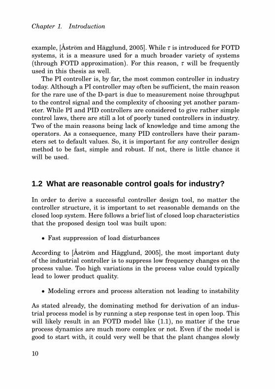
i.e. processes with complex poles. In particular when T = 0.1 the newIAE is as small as 62.5% of the MIGO IAE, corresponding to a signif-icant improvement. Figure 4.10 shows the output signal, y, and con-trol signal, u, when a load disturbance, d, is acting on the process in-put. The dashed curves correspond to the MIGO controller (K = 3.96,Ti = 0.46, Td = 0.08), the solid lines to the proposed controller withthe M -circle constraint (K = 5.42, Ti = 0.29, Td = 0.16) and the dash-dotted line to the new design method with the Ms- and Mp-constraints(K = 6.53, Ti = 0.22, Td = 0.16). The open loop Nyquist curves forthe three cases are shown in Figure 4.11. It is known that the MIGO
48

4.4 Examples
0 0.2 0.4 0.6 0.8 130
40
50
60
70
80
90
100
100
⋅IAEMs,Mp/IAEM
Normalized time delay τ
Figure 4.9 The IAE-values for the test batch was compared using either theM -circle constraint alone or both the Ms- and Mp-circle. The plot displays 100 ⋅
IAEMs,Mp/IAEM as a function of the normalized time delay τ .
method discards solutions that touches the M -circle twice. This exam-ple shows that this choice may be overly conservative. It is also evidentthat the substitution of the M -circle to the Ms- and Mp-circles gives amuch lower IAE-value in this case.
The previous example showed that the program works well and thatit has the potential to give birth to new findings on PID control. It isalso a lot easier to start using than the MIGO method, which reliesmore on the user.
49
Chapter 4. A Software Tool for Robust PID Design
0 0.5 1 1.5 2 2.5 3 3.5 4
−1
−0.8
−0.6
−0.4
−0.2
0
0.2
0 0.5 1 1.5 2 2.5 3 3.5 4−0.05
0
0.05
0.1
0.15
0.2
yu
Time (s)
Time (s)
Figure 4.10 Output (y) and control signal (u), during a load disturbance, forthree different designs on (4.12), T = 0.1. Dashed line: MIGO PID; Solid line:Proposed PID with M -circle constraint; Dash-dotted line: Proposed PID with theMs- and Mp-circle constraints.
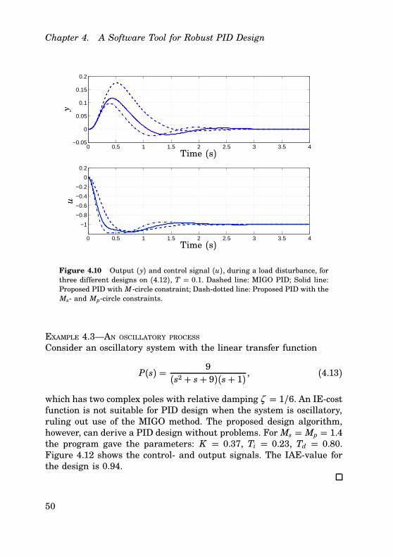
EXAMPLE 4.3—AN OSCILLATORY PROCESSConsider an oscillatory system with the linear transfer function
P(s) = 9(s2 + s+ 9)(s+ 1) , (4.13)
which has two complex poles with relative damping ζ = 1/6. An IE-costfunction is not suitable for PID design when the system is oscillatory,ruling out use of the MIGO method. The proposed design algorithm,however, can derive a PID design without problems. For Ms = Mp = 1.4the program gave the parameters: K = 0.37, Ti = 0.23, Td = 0.80.Figure 4.12 shows the control- and output signals. The IAE-value forthe design is 0.94.
50

4.4 Examples
−2 −1.5 −1 −0.5 0 0.5−1.5
−1
−0.5
0
0.5
1
Real Axis
Imag
inar
y A
xis
Figure 4.11 The open loop Nyquist curves when three different design meth-ods were used on (4.12), T = 0.1. Dashed line: MIGO control; Solid line: Proposeddesign with M -circle constraint; Dash-dotted line: Proposed design with the Ms-and Mp-circle constraints.
0 5 10 15−0.2
0
0.2
0.4
0.6
0 5 10 15
−1
−0.5
0
yu
Time (s)
Time (s)
Figure 4.12 Output signal, y, and control signal, u, when the proposed designmethod was used to find a controller for the oscillatory process (4.13). Ms =Mp = 1.4.
51

5
Adjustable Control Signal
Noise Reduction
Methods like MIGO/AMIGO and lambda tuning have the weaknessthat they have no systematic way of designing the low-pass filter act-ing on the measurement signal or the D-part. The same goes for theapproach described in Chapter 4 where the effect of the low-pass fil-ter was completely ignored. Designing PID controllers without roll-offcan give severe throughput of measurement noise in the control signalfor a real plant. This chapter will, therefore, introduce a new way oftuning the low-pass filter such that the control signal variance, dueto measurement noise, is constrained. Or in other words, choosing T fsuch that
qSkq22 =∥
∥
∥
C
1+ PC∥
∥
∥
2
2= σ 2u
σ 2n≤ Vk. (5.1)
Sk is the transfer function from measurement noise n to control signalu, σ 2u is the variance of the control signal and σ 2n is the variance of themeasurement noise. Vk is a design variable that is user specified.This chapter will begin with a description of the principles of the
new design method. There are also several new challenges associatedwith the proposed method, which will be presented in a section of itsown. Finally, the chapter will be concluded by a suggestion of designalgorithm together with several examples on the use of the method.But, first of all, a short note on the software tool.
52

5.1 Principle
Designing discrete time controllers for real plants
Even though controllers have to be implemented digitally, most PIDdesign methods are based on continuous time analysis only. The PIDparameters are then used directly in a discrete time approximationof the controller when implemented. Such an approximation will, how-ever, introduce phase lag (see e.g. [Åström and Wittenmark, 1997]) andis thus likely to make the closed loop system less robust than intended.This problem will be especially severe if the sampling time assigned tothe process has been chosen too long by mistake. This could very wellbe the case in industry, which will be shown in Chapter 6. For thesereasons, a discrete time version of the design software has been devel-oped in parallel with the continuous time version. While the previouschapter was all about the continuous time version, the discrete timesoftware will mainly be used in this chapter.The discrete time controllers have been approximated with forward
Euler on the I-part, backward Euler on the D-part - according to [Årzén,1996] - and Tustin’s approximation on the low-pass filter such that thefinal PID controller becomes
C(z) = K(
1+ 1
Tiz−1h
+ Tdz− 1zh
)
⋅1
(
1+ 2(z−1)h(z+1)Tf +
(
2(z−1)h(z+1)Tf
)2/2) .
The PI controller is very similar.The discrete time version of the software is not yet released. Anyone
can, however, take the program and redo it in the same fashion. Fewchanges are needed from the original version.
5.1 Principle
The idea for finding a controller that fulfills constraint (5.1) will beillustrated through an example.
EXAMPLE 5.1—THE RELATION BETWEEN Tf AND VkDetermining the variance ppSkpp22 for a lot of different Tf -values (using
53

Chapter 5. Adjustable Control Signal Noise Reduction
0 0.2 0.4 0.6 0.8 1 1.2 1.4 1.60
2
4
6
8
10
12
14
16
18
20
Tf
Vk
P1
P2
P3
P4
Figure 5.1 Different processes give similar dependencies between T f and thecontrol signal variance.
the proposed Matlab software) on the systems
P1(s) =1s+ 1 e
–s, P2(s) =1
(s+ 1)2 e–s,
P3(s) =1
(s+ 1)4 , P4(s) =(−0.5s+ 1)(s+ 1)3 ,
have shown that there are very similar dependencies between T f andVk in all four cases, see Figure 5.1. Having relations like these makesit possible to use T f as a design variable to fulfill (5.1).Finding the T f that gives a certain Vk can be done using differentsearch methods. Another approach, and the one that will ultimately beused in this thesis, is to determine the relation between performance(IAE) and noise amplification (Vk). That way, the control designer can
54

5.1 Principle
0 2 4 6 8 10 121.8
1.9
2
2.1
2.2
2.3
2.4
2.5
2.6
2.7
Vk
IAE
Figure 5.2 Trade-off curve between noise amplification and performance forthe process P1, in Example 5.1. Note that the noise characteristics used herewas not the same as in Figure 5.1, which explains the difference in Vk-values.
take the trade-off between noise throughput and performance into ac-count when choosing a suitable controller. Figure 5.2 shows an exampleof this relation for process P1.There are also some other interesting effects one can analyse after
adding the new constraint into the picture. Like for instance:
• For which types of systems will the D-part be most important?
• When will the low-pass filter make the least difference?
Here is one example showing some interesting effects.
55

Chapter 5. Adjustable Control Signal Noise Reduction
Table 5.1 The effect of the low-pass filter time constant on the control of firstorder systems with time constant T and delay L = 1. Vk was set to 1.
T h (s) K Ti Td T f IAEinc (%)
0.1 0.02 0.21 0.42 0.14 0.014 0.7
1 0.05 0.59 1.04 0.44 0.13 12.6
50 1.5 2.44 21.8 11.4 12.4 1647
EXAMPLE 5.2—FOTD SYSTEMS WITH VARIANCE CONSTRAINT
Take three FOTD systems
P(s) = 1Ts+ 1 e
–s, T = 0.1, 1, 50,
which have τ = 0.91, 0.5 and 0.02 respectively. Assume furthermorethat the measurement noise in all three cases is white, unit variance,noise (each sampled with different sampling time h). As will be ex-plained in Section 5.2, it is not trivial to compare different systems, sothese three cases will be treated without comparison.Vk will be set to 1 when designing controllers for all three pro-
cesses, such that the control signal get the same variance as the whitemeasurement noise. Table 5.1 shows the results when designing PIDcontrollers as described in the previous section. The table displays sam-pling time, PID parameters, low-pass filter time constant as well asIAE increase compared to an unfiltered controller. Figure 5.3 showsthe Bode plots of all three PID controllers.Analysing the results, one can see that the most lag dominant sys-
tem (T = 50) has the biggest increase in IAE compared to when thecontroller does not include a measurement filter. This relates to whatexamples from the previous chapter said about lag dominant systemsbeing the most sensitive to changes in the optimization problem. Itseems like the same holds for when the variance is limited. Severalsimilar runs have shown that this example is in no way particular inthis aspect. The performance of lag dominant systems are generallysensitive to changes, which also makes them quite hard to analyse.Delay dominant systems, on the other hand, are barely affected at all
56

5.1 Principle
10−2
10−1
100
101
102
10−2
10−1
100
101
102
Frequency (rad/s)
Mag
nitu
de
10−2
10−1
100
101
102
−80
−60
−40
−20
0
20
40
60
80
Frequency (rad/s)
Pha
se (
degr
ees)
T=0.1T=1T=50
Figure 5.3 Bode diagrams of the PID controllers for the three FOTD systemsin Example 5.2.
by the low-pass filter, which would pretty much mean that one can addthe filter after the controller design if one would want to.Another very interesting feature, is that the PID controllers for lag
dominant systems are more similar to PI- or even I-controllers. In thisexample, it can be seen both in the Bode plots and by comparing Tdand T f which are very close. In other words, the low-pass filter rolls offclose to the frequency where the D-part starts to increase the gain.
Motivation of the constraint and options
It has already been mentioned that one of the main reasons for notincluding the D-part in industry is because it makes the control sig-nal sensitive to measurement noise. Highly fluctuating control signalsare likely leading to wear and tear on actuators, which are typicallyvery expensive to exchange. This is the main reason for including the
57

Chapter 5. Adjustable Control Signal Noise Reduction
variance constraint in this chapter. Such a constraint will capture thevariation of the control signal and make the designer able to use theD-part without fear of getting too much noise throughput.One disadvantage with using the variance constraint as a measure
is that it does not weigh in for which frequencies the sensitivity is high.A low frequency sine wave can for instance have the same variance asa swiftly shifting noise signal. It does, however, seem more likely thathigh frequency components in the noise will wear on actuators ratherthan the low frequency part. For that reason it is a good idea to weighSk with respect to frequency. In this thesis this will be done by high-pass filtering measurement data to try to single out the measurementnoise (see Section 5.2). Whether or not this is enough to get the desiredcharacteristics for the closed loop system will be left for future work toshow.Another option for a constraint is what was used by for instance
[Kristiansson and Lennartson, 2006], namely qSkq∞. This gives a limiton how much any frequency can be amplified. The measure is quitestraight forward, but it would ideally need weighting depending onfrequency, just like the variance constraint. There is little point inlowering the peak of Sk for low frequencies.Instead of the variance, one could just as well have constrained
the standard deviation or the quantiles of the signal. Both measuresare related to the variance. The standard deviation has a more directrelation to the magnitude of the control signal than the variance. Usingquantiles would mean that one can specify how large quantity of thecontrol signal would lie outside a certain limit. This would possibly bea more easily explainable measure to people in industry. Nevertheless,the choice of constraint fell on variance for this thesis. It can, however,easily be translated into these other two quantities.
Why is the method not optimal?
It is important to realize that fulfilling constraint (5.1), choosing aTf giving a certain Vk, will not give controllers that are optimal withrespect to the constraint. The software calculates controllers that areoptimal with respect to the two robustness constraints, given a certainTf . It could, however, very well be that a different T f could give evenlower IAE, using other controller parameters that alters qSkq22. Oneexample could be a controller derived with a certain T f that results in
58

5.1 Principle
too high variance. A little less aggressive controller, but with the sameTf , may still give less IAE than the controller which the proposeddesign method chooses.In Section 4.3 it was shown that unless the control signal variance
constraint is taken into account, the PID controller can be quite supe-rior to the PI controller regarding IAE. The D-part in a PID controllerwill, however, also give a significant raise to the control signal vari-ance due to measurement noise. Therefore, it is not so straightforwardto assume that a controller always benefits from having a D-part. Itis rather a combination of process characteristics and the amount ofcontrol signal variance allowed that will determine the usefulness ofthe D-part.Depending on the sampling time, it may not be possible for the
control signal variance to reach the Vk that has been set (see Figure5.4). The reason being that the low-pass filter cut-off frequency wouldhave to be so far beyond the Nyquist frequency to give Vk that it justdoes not affect the variance enough. This is not necessarily negative,but shows that one could perhaps have used a different controller forwhich Vk is higher and the IAE is lower.The fact that the PI controller may give a control signal variance
lower than Vk makes it a bit difficult to compare with the PID con-troller. But, it is logical to let the PID controller take whatever T fgives Vk, even if the PI controller gives qSkq22 < Vk, when comparing.After all, it is the user that sets the rules and even if both controllerscan not reach the limit, they are both playing by the rules.Assume that one wants to examine the behaviour of the following
two systems
P1(s) =e–s
(10s+ 1)2 , P2(s) =e–s
(50s+ 1) ,
with respect to control signal variance, using both PI and PID control.The sampling time has been chosen to h = 0.01 seconds with Ms =Mp = 1.4 in both cases. In Figure 5.5, the IAE-values are plotted versusqSkq22 for a number of different T f -values. The curves reveal that thePI controller can actually have lower IAE value than the PID controllerwhen the control signal variance, qSkq22, is the same. For P1(s), thisoccurs when Vk ( 0.002 and for P2(s) when Vk ( 1.75. These results
59

Chapter 5. Adjustable Control Signal Noise Reduction
0 0.005 0.01 0.015 0.02 0.025 0.03 0.035 0.040
0.05
0.1
0.15
0.2
0.25
0.3
0.35
0.4
0.45
Tf
||Sk|| 22
Figure 5.4 PI control of G(s) = (s + 1)–3 with different choices of T f is notnecessarily able reach qSkq22 = Vk. In this case for instance, qSkq22 does not takelarger values than 0.42. The measurement noise is here assumed to be white,unit variance, sampled with h = 0.01s.
lead to two conclusions: The PID controller is not optimal for the newoptimization problem and the closed loop system around P2 seems tobenefit quite a lot less from the D-part than the P1 loop does.Now that it is known that the selected controllers are not optimal,
one could ask a few justified questions: When would it be smart toswitch to PI control? Are the controllers one gets through the proposedmethod still good enough to use? How far from optimality will the PID(or PI) controllers be? These are questions that to some extent willhave answers at the end of this thesis. In this section, there will be anattempt to answer the first question.Analysis of the controllers for P1 and P2 shows that there seems to
be at least one measure that gives an indication of when it is a goodidea to check how well a PI controller would work. That measure is therelation between Tf and Td of the final PID controller. Figure 5.6 showsTf /Td plotted versus T f for P2(s). At T f ( 0.8, this quotient comes veryclose to 1, meaning that the final PID controller is pretty much a PIcontroller. When comparing this Tf value to the ones in Figure 5.5 for
60

5.2 Challenges with the use of a variance constraint
10−4
10−2
100
102
104
106
0
5
10
15
20
25
30
35
40
45
||Sk||2
2
IAE
PI, P1
PID, P1
PI, P2
PID, P2
Figure 5.5 Processes P1 and P2 were run with several different T f -valuesusing h = 0.01s. This gave the following relation between IAE and control signalvariance, showing that the PID controllers are not necessarily optimal.
when the PI is better than PID, it shows that for Tf ( 1.15 and above,the PI controllers are better. This is rather close to 0.8. Experimentson several other processes in the AMIGO batch have shown that this isa repeating behaviour for the cases when PI is preferable. Therefore, itseems like a good idea to first run the PID design and then, if T f/Td (1, also run the PI algorithm to see if that gives an even better result.When thought through, it seems quite logical that as Vk goes to zero,the controller will be given less freedom to increase the gain and phase,thus becoming more and more like a PI controller or even a pure Icontroller for that matter.
5.2 Challenges with the use of a variance constraint
Using variance as a measure of when the control signal is sensitive tomeasurement noise is in many ways a simple and intuitive. But therealso comes quite a few challenges together with using the constraint.Some of these will be presented in this section.
61

Chapter 5. Adjustable Control Signal Noise Reduction
0 5 10 15 20 25 30 350
0.2
0.4
0.6
0.8
1
1.2
1.4
Tf
Tf/T
d
Figure 5.6 Designing several PID controllers with different T f for processP2(s) shows that these are almost PI controllers when T f reaches a certainvalue (and qSkq22 decreases). Checking if T f /Td ( 1 can then be a measure tosee when it is a point in switching to PI control.
How to calculate the variance?
In order to get a good estimate of the real variance relation σ 2u/σ 2n onewill first need a representative selection of noise data. One possibilityis to run the process in open loop, log the measurement data and thenfilter out what is assumed to be the noise. Logging the data couldbe done either by having the system run in manual with a constantcontrol signal or in connection to a step response test on the process.The latter option seems more attractive since these kinds of tests areoften run on a process to determine an FOTD model just before thecontroller design. It would thus be a very natural way to incorporatenoise logging in the normal procedures of controller design. Anotheroption would be to get the data either through relay tests, which arecommon in auto-tuning, or through closed loop runs. If it is possibleto derive good noise data like this it would be advantageous, since the
62

5.2 Challenges with the use of a variance constraint
process should ideally be in closed loop all the time. In this thesis,however, it will be assumed that the measurement data is collected inopen loop.Now assume that one can collect a sequence of representative noise
data. How long does this log need to be in terms of time in orderto provide a good sample for estimation of the variances? And whatmethod should be used to calculate σ 2n and σ 2u? There will not be anyreal analysis in this thesis trying to answer the first question. Butit seems reasonable to believe that, if the step response is used tocollect noise data, it will depend on how fast the process is. If theprocess is fast, one may need to hold the process a little longer inopen loop to gather some more noise data. Since one may get very longmeasurement logs for a process with slower dynamics, it is more likelythat the length of the noise data will be sufficient in this case. If thenoise data is extensive enough, it should be fine to calculate the noisevariance simply by using the formula
σ 2n =1N
N∑
i=1(ni − n)2,
where N is the number of noise data, n, and n is the mean value ofthis data. Another option is to determine a model, N, of the noise suchthat
n(k) = N(q)e(k)where e is white noise. This model can then be used to estimate σ 2u aswell. This approach will be used here when Youla parametrized con-trollers are compared to PI/PID controllers. When running the PI/PIDdesign on a real process, however, the actual noise data will be usedas part of a Simulink simulation to estimate σ 2u. The advantage withthe model approach is that it allows for better analysis, but it is badin practise since one needs to automatize the model making which isnot trivial. Using the real data is a much easier method. On a whole,it should be part of future research to look more at how to get repre-sentative information of the measurement noise.
How to disregard other sources when gathering noise data?
Assume that one wants to extract the measurement noise out of anopen loop run on the system. What part of the signal should be kept
63

Chapter 5. Adjustable Control Signal Noise Reduction
and which can be thrown away? [Marlin, 1995] points out that thevariations showing in the measurement data are a result of severaleffects. Some of them come from the process itself, some from the sen-sors, while others are due to transmission. All these effects contributeto the signal over a wide range of frequencies. The idea of the proposedmethod is to be able to set the control signal variance such that thewear on actuators, like valves, can be kept low. Generally speaking, itis, large, high frequency movements in the control signal that leadsto this wear. Therefore, the idea is to weigh the measurement data bysending it through a high-pass filter, W(s). The low-frequency part ofthe data is thus assumed to have small contribution to actuator wear.The high-pass filter
W(s) = s2
s2 + 2ζ ω os+ω 2o, (5.2)
was chosen for this reason. It is discretized, with the current samplingtime of the process, before the measurement data is run through it. Thedamping coefficient ζ was set to 0.7 to receive a filter that is steep,but still does not give much overshoot in a Bode magnitude diagram.Since the filtering is handled offline, one can use non-causal filtersthat are almost ideal high-pass filters. But, since the hardest questionis how to choose ω o properly, it seems like a good idea to keep some ofthe lower frequencies in the filtered data as well.The noise data can roughly be divided into controllable distur-
bances, uncontrollable disturbances and measurement noise. Thesethree sources will to some degree overlap each other, but it seems rea-sonable to assume that the measurement noise throughput will mainlywear on actuators for frequencies above the cut-off frequency of theclosed loop. In many industrial systems, the closed loop is rarely fasterthan the process itself. For that reason it is a possibility to choose ω o todepend on the process model. If the process model is an FOTD system,ω o could for instance have a default value of 3/T , where T is the timeconstant of the process. The user should, however, be ready to changethis value from case to case.
Sampling time issues
When making discrete time controllers, the sampling rate will be dif-ferent depending on the process. Too slow sampling could introduce
64

5.2 Challenges with the use of a variance constraint
unnecessary phase lag, thus decreasing the best possible performancesignificantly. Really fast sampling may on the other hand not be pos-sible, due to for instance resource limitations. So, generally speaking,one should strive to choose sampling time from case to case. This does,however, also give some additional effects in connection to the varianceconstraint that are important to be aware of if one wants to comparenoise effects on different processes.Assume that one has a certain sensitivity function Sk(s) for some
closed loop system. This system is sampled with the two different sam-pling times h1 and h2. The variance relation between the continuoustime system and the sampled time systems is
hiqSki(s)q22 = qSki(z)q22,
when zero order hold sampling is used. The index i refers to the dif-ferent sampling rates. The control signal variance should, however, bealmost the same for both sampling cases, as long as the sampling rateis chosen properly to avoid aliasing. In other words, energy should beconserved. It was also shown that, on a water tank process (see Section5.4), the relation σ 2u/σ 2n was almost constant for two different samplingrates. The controller was the same in both cases. This observation gives
∥
∥
∥
Sk1(z)√h1
∥
∥
∥
2
2=∥
∥
∥
Sk2(z)√h2
∥
∥
∥
2
2,
which will force the relation
qSk1(z)q22 =∥
∥
∥
√
h1
h2Sk2(z)
∥
∥
∥
2
2=∥
∥
∥
√
1JSk2(z)
∥
∥
∥
2
2,
between the two cases. J = h2/h1 and corresponds to an up- or down-sampling ratio. It is very important to take the J-ratio into accountwhen designing controllers. If not, variance will depend heavily onsampling rate, such that qSk(z)q22 → 0 as h→ 0. Figure 5.7 shows PIDdesigns for
P(s) = 1(50s+ 1) e
–s (5.3)
65

Chapter 5. Adjustable Control Signal Noise Reduction
10−2
10−1
100
100
101
102
Frequency (rad/s)
Mag
nitu
de
10−2
10−1
100
−150
−100
−50
0
50
Frequency (rad/s)
Pha
se (
degr
ees)
h=0.75h=1.5h=2.0
Figure 5.7 Three PID controllers determined for process (5.3) with Vk ( 1,but sampled with different sampling time h.
using three different sampling times h = 0.75, 1.5 and 2 seconds. Themeasurement noise was assumed to be white, unit variance, noise sam-pled with h = 0.01 seconds. Using the noise sampling time as h1 refer-ence, this resulted in down-sampling ratios of J = 0.75/0.01 = 75, 150and 200 respectively. As one can see, taking Vk ( 1 gave very similarcontrollers. Performance was also almost the same in all three cases.If J had not been taken into account, however, the controllers wouldhave been very different, depending on sampling time. In Example 5.2,this ratio was not part of the design and one could thus not comparethe different designs directly. From now on, when comparing designson different systems, J will be part of the procedure. In reality, how-ever, one will not need to think about this when using the proposedmethod. There will only be a series of measurement data which canthen be used to form a noise model or be directly used in simulationestimations.
66

5.3 Suggested procedure for design of PID controllers on real processes
5.3 Suggested procedure for design of PID controllerson real processes
Below follows one suggestion on how to design PI or PID controllersfor real processes.
1. Collect noise data from the process, detrend it and estimate thevariance σ 2n.
2. Choose a number of different T f values. For each T f :
• design a PI or PID controller using the proposed software.
• simulate the closed loop system using the gathered noisedata and estimate the variance, σ 2u, of the control signal.
3. Plot IAE versus Vk (like in Figure 5.2) to get a picture of howmuch performance costs in terms of measurement noise through-put to the control signal.
4. Choose a suitable controller from the given set, taking the trade-off curve into consideration.
This new method ought to give the user a systematic way of bringingthe D-part of the PID controller into industrial controller design. Thestructure of the controller should, however, be determined with respectto what specifications are set on the process and not be chosen inadvance. A PI controller should thus be chosen if it is better suitedthan a PID and vice versa.It would also be a good idea to have some software that automatizes
the procedure. The user should, however, be able to modify parameterslike ω o and Vk. A set of different controllers should be kept in caseone would later want to change how sensitive the control signal is tomeasurement noise.
5.4 Examples
This section will contain three simulated and one real example of howthe proposed design method can be used. Youla parametrized con-trollers will be derived for comparison with the PI and PID controllers.
67

Chapter 5. Adjustable Control Signal Noise Reduction
The three examples, in which simulations are used, will be assumedto have white measurement noise, with unit variance, acting on theprocess value. In the first example, three processes will be comparedas described in the sampling issues part of Section 5.2. In other words,they will be assumed to have the same, but differently sampled, whitemeasurement noise. The other two simulated examples will have mea-surement noise with the same sampling time as the process is sampledwith. The three examples can therefore not be related to one another.It will be left to Chapter 7 to deal more with comparisons like that.Before the examples are presented, the IAE measure will be dis-
cussed a bit.
Performance measure for time delayed systems
Assume that a process has a time delay of L = 1 second. This meansthat it will take one second until a load disturbance on the control sig-nal shows up in the measurements. It will then take one more secondbefore the control signal can affect the process value. So, no matterwhich controller is used, it will always take two seconds until the con-trol signal can alter the process value. This will correspond to a fixamount of IAE that can not be reduced. Depending on how fast andtime-delayed the system is, this part of the IAE may very well be themajority of the full IAE. This is especially true for systems with τ ( 1.Comparing two different controllers with the standard IAE measurecould therefore give a false picture of how close they are in perfor-mance. For this reason, only the remaining part of the IAE, IAEu (udenotes IAE affected by the control signal) will be used in the first ofthe simulated examples in this section. The new measure will, however,not be used for the real process example.
The examples
EXAMPLE 5.3—FIRST ORDER TIME DELAYED PROCESSESPID- and Youla parametrized controllers were derived for the threedifferent FOTD processes,
P1(s) =e–s
0.1s+ 1, P2(s) =e–s
s+ 1, P3(s) =e–s
500s+ 1,
68

5.4 Examples
Table 5.2 Results when PID and Youla controllers were derived for threedifferent FOTD systems.
P1 P2 P3
K 0.21 0.61 28.3
Ti 0.42 1.01 44.6
Td 0.13 0.41 0.00
T f 0.0074 0.06 2.58
IAEPIDu 1.09 1.51 1.62
IAEYoulau 0.61 1.20 1.38
IAEincu 78% 26% 17%
where P1 is delay dominant (τ = 0.91), P3 lag dominant (τ = 0.002)and P2 is somewhere in between, with τ = 0.5. In all three cases,Vk was set to 1 although it was weighted with the down-samplingfactor J as described before. The three systems were given differentsampling times hP1 = 0.02 s, hP2 = 0.05 s and hP3 = 5 s. The whitemeasurement noise was assumed sampled with h = 0.01 seconds. Inother words, J = 2, 5 and 500 respectively. Table 5.2 shows data fromeach of the three cases. The order of the Q-filter was 140 in all threeYoula optimizations. Note that for P3, a PI controller is given insteadof a PID for the reasons mentioned in Section 5.1. The PID was, in thiscase, 27% worse than the PI controller regarding IAEu. Let us now gointo more detail on the different control loops.Figure 5.8-5.13 shows the Bode diagrams and load disturbance re-
sponses of the PI/PID- and Youla controllers respectively for each ofthe three processes. The PID controller for P1 gives an IAEu that is78% higher than that of the Youla controller. This is by far the biggestdifference of the three. Looking at the load disturbance response (Fig-ure 5.9), it is obvious that the great potential of the Youla controllermakes it quite a lot better performance wise than the PID. The Youlacontroller does, however, have several peaks in the Bode diagram re-sulting in a major phase advance. While this is the secret to the grandcontrol, it is also likely to give very bad robustness towards time de-
69

Chapter 5. Adjustable Control Signal Noise Reduction
10−1
100
101
102
10−1
100
101
102
Frequency (rad/s)
Mag
nitu
de
PIDYoula Controller
10−1
100
101
102
−200
−100
0
100
200
300
400
500
Frequency (rad/s)
Pha
se (
degr
ees)
Figure 5.8 Bode diagram of the PID and Youla controllers for process P1 inExample 5.3.
0 1 2 3 4 5 6 7 8 9 10−0.2
0
0.2
0.4
0.6
0.8
1
1.2
Time (s)
Pro
cess
Val
ue
PIDYoula Controller
0 1 2 3 4 5 6 7 8 9 10−1.2
−1
−0.8
−0.6
−0.4
−0.2
0
0.2
Time (s)
Con
trol
Sig
nal
Figure 5.9 Load disturbance responses when the PID and Youla controllersare used respectively on process P1 in Example 5.3.
70

5.4 Examples
lay variations. A small error in the modeled delay could potentiallymake the closed loop system unstable. Therefore, it would be advis-able to have additional constraints put on the Youla optimization inorder to compare systems really thoroughly. Adding such a constraintis, however, not trivial since it has to be closed loop convex. Given this,the PID controller may not give such a bad result after all and onecould argue that a PI controller would be even better to use. The PIcontroller is only able to reach qSkq22 = 0.02. Its IAEu-value of 1.39is, however, only 28% higher than that of the PID controller. So, onegets an even less advanced controller with this rather small decreasein performance. It is also a known trick to switch off the D-part whencontrolling delay dominant processes (see for instance [Hägglund andÅström, 1991]). For P2, there are still some peaks left in the Bode plotof the Youla controller (see Figure 5.10) although not quite as pro-nounced as for P1. The performance gain in using the Youla controlleris quite a lot smaller than for P1, where IAEu of the PID is just 26%off. The two load disturbance responses in Figure 5.11 are also quitesimilar with the biggest difference being the small undershoot of theYoula controller. This indicates that the PID controller is a valid choicein this specific case. With process P3 (see Figures 5.12 and 5.13), a PIcontroller actually ends up giving better IAEu than the correspondingPID controller (27% higher in this specific case), when using the pro-posed design method. Taking a look at the Youla controller should givea good hint of why this has happened. The best linear controller isbasically a PI controller. This gives a hint that an alternative way ofdesigning the controller could be to:
1. Derive a balanced model of the Youla controller
2. Reduce the new model, looking at the Hankel singular values
This way, one would end up with a good controller of low order, whichdoes not depend on any beforehand given structure. One example ofthis type of reduction is given in Example 5.5 and another can befound in [Norman and Boyd, 1989].It could be that the careful reader reacts to the PI control parame-
ters being a bit too aggressive for P3. This is, however, merely an effectof the measurement noise being down-sampled by quite a lot comparedto the other two processes. On a real process it should never be a prob-
71

Chapter 5. Adjustable Control Signal Noise Reduction
10−2
10−1
100
101
10−1
100
101
102
Frequency (rad/s)
Mag
nitu
de
PIDYoula Controller
10−2
10−1
100
101
−100
−50
0
50
100
150
200
250
300
350
400
Frequency (rad/s)
Pha
se (
degr
ees)
Figure 5.10 Bode diagram of the PID and Youla controllers for process P2 inExample 5.3.
0 5 10 15−0.1
0
0.1
0.2
0.3
0.4
0.5
0.6
0.7
Time (s)
Pro
cess
Val
ue
PIDYoula Controller
0 5 10 15
−1
−0.8
−0.6
−0.4
−0.2
0
0.2
Time (s)
Con
trol
Sig
nal
Figure 5.11 Load disturbance responses when the PID and Youla controllersare used respectively on process P2 in Example 5.3.
72

5.4 Examples
10−2
10−1
100
101
102
103
Frequency (rad/s)
Mag
nitu
de
PIDYoula Controller
10−3
10−2
10−1
−90
−80
−70
−60
−50
−40
−30
−20
−10
0
Frequency (rad/s)
Pha
se (
degr
ees)
Figure 5.12 Bode diagram of the PID and Youla controllers for process P3 inExample 5.3.
0 20 40 60 80 100 120 140 160 180 200−0.005
0
0.005
0.01
0.015
0.02
0.025
0.03
Time (s)
Pro
cess
Val
ue
PIDYoula Controller
0 20 40 60 80 100 120 140 160 180 200−1.4
−1.2
−1
−0.8
−0.6
−0.4
−0.2
0
Time (s)
Con
trol
Sig
nal
Figure 5.13 Load disturbance responses when the PID and Youla controllersare used respectively on process P3 in Example 5.3.
73

Chapter 5. Adjustable Control Signal Noise Reduction
lem. The controller will only be aggressive if the measurement noiseand user allow for it.Once again, the measure T f /Td can be used to get an indication
of when a PI controller is preferred. For the PID controller on P3,Tf /Td = 4.72/2.83 = 1.67, which is quite high above 1.The Youla controller for process P3 confirms that, for a lag dominant
FOTD, it is less likely that the D-part is valid than for a more delaydominant system. It also shows that it is reasonable to only have afirst order low-pass filter on the PI controllers derived from the PIDsoftware. Another interesting fact is that all three Youla controllershave some sort of roll-off. This gives a hint that a PID controller withsecond order low-pass filter is the preferred choice of structure. Inindustry, however, it is most common to use filters of order one.Youla parametrization with a finite FIR filter will provide a con-
troller that is approximately the best linear controller. Or rather, it isthe optimal controller for the set of controllers that can be created withthe given Q-filter. The higher the order of the Q-filter is, the betterthe approximation of the optimal linear controller will be, such thatit is close to the limit of performance. In the cases considered here,one can get an estimate of how close the Youla controllers are to thislimit by plotting IAEu versus the filter order, NQ . Figure 5.14 showsthis relation for process P2. NQ = 73 was the smallest value givingan integrator in the controller. As can be seen, the IAEu changes verylittle for NQ greater than 120. This gives an indicator that the Youlacontroller, for which NQ = 140, gives an optimum close to the limitof performance and it will therefore be a good approximation of thebest linear controller. Besides, the difference between the highest andlowest IAEu is, in fact, only 9%. P1 and P3 have similar looking plotsto Figure 5.14. Making these plots is also a fairly fast way of makingsure that the Youla controller quality is good.
EXAMPLE 5.4—FOURTH ORDER LAG PROCESSThe fourth order lag process
P(s) = 1(s+ 1)4
was investigated in the same fashion as the FOTD systems in theprevious example. Vk was initially set to 1, when using a sampling time
74

5.4 Examples
60 80 100 120 140 160 180 200 2201.18
1.2
1.22
1.24
1.26
1.28
1.3
NQ
IAE
u
Figure 5.14 The relation between IAEu and the order of the Q-filter for pro-cess P2 in Example 5.3 indicates that the solution of the Youla optimizationcomes close to the limit of performance.
of h = 0.25 seconds and a Q-filter of order 150. Bode plots and loaddisturbance responses for the PID and Youla controllers are shown inFigure 5.15 and 5.16. The designed PID controller has the parametersK = 0.73, Ti = 2.38, Td = 1.29 and Tf = 0.52, with IAE = 4.06. Thiscan be compared to the IAE of the Youla controller which is 3.43. ThePID controller thus gives about 18% higher IAE compared to the bestpossible linear controller. Considering this and how similar the loaddisturbance responses look, one gains fairly little from having a moreadvanced controller than PID in this case.Now consider how the Youla controller alters with varying Vk. Fig-
ure 5.17 shows the Youla controllers when Vk = 5, 1, 0.2 and 0.04.The difference in IAE from the PID counterpart goes from 28 % whenVk = 5 to basically 0 % when Vk = 0.04. Looking at the Bode diagram,it is apparent that the controllers get less freedom for lower Vk-values.The resemblance also goes first towards PID controller and then PI,
75

Chapter 5. Adjustable Control Signal Noise Reduction
10−2
10−1
100
101
10−2
10−1
100
101
102
Frequency (rad/s)
Mag
nitu
de
PIDYoula Controller
10−2
10−1
100
101
−100
−80
−60
−40
−20
0
20
40
Frequency (rad/s)
Pha
se (
degr
ees)
Figure 5.15 Bode diagrams of the PID and Youla controllers for the fourthorder lag process in Example 5.4.
0 5 10 15 20 25 30 35−0.1
0
0.1
0.2
0.3
0.4
0.5
0.6
0.7
Time (s)
Pro
cess
Val
ue
PIDYoula Controller
0 5 10 15 20 25 30 35
−1
−0.8
−0.6
−0.4
−0.2
0
Time (s)
Con
trol
Sig
nal
Figure 5.16 Load disturbance responses when the PID and Youla controllerare used respectively on the fourth order lag process in Example 5.4.
76

5.4 Examples
10−2
10−1
100
101
10−2
10−1
100
101
Mag
nitu
de
Frequency (rad/s)
10−2
10−1
100
101
−100
−80
−60
−40
−20
0
20
40
60
Frequency (rad/s)
Pha
se (
deg)
Vk=5
Vk=1
Vk=0.2
Vk=0.04
Figure 5.17 Fourth order lag process: Youla Controllers for four different val-ues on Vk. As Vk decreases, the controller gradually becomes more and moresimilar to a PI controller.
when Vk is really small. For even lower values on Vk, it could even bethat an I controller would be preferred. This means that the preferredcontroller structure depends on what expectations one has on the con-trol signal variance. The level of variance at which a more advancedcontroller is preferred does of course vary from process to process.
EXAMPLE 5.5—AN OSCILLATORY PROCESSThe next process to be examined is
P(s) = 9(s2 + s+ 9)(s+ 1) ,
which was previously considered in Section 4.4. It is a highly oscillatoryprocess, having two poles with relative damping ζ = 1/6, known togive PID controllers trouble to quickly damp out load disturbances.
77

Chapter 5. Adjustable Control Signal Noise Reduction
The process was run with Vk = 1, h = 0.1 seconds and a Q-filter oforder 150. This gave the two controllers shown in Figure 5.18, withthe load disturbance responses in Figure 5.19. The PID controller hasK = 0.30, Ti = 0.30, Td = 0.43 and T f = 0.06 giving IAE = 1.44.The IAE of the PID is 48% higher than that of the Youla Controller(IAE = 0.97). This is a more distinct difference than most of the othercases investigated so far. The Youla controller is also free from the highpeaks that characterized the controller for process P1 in Example 5.3.If Vk is set to a higher value, the Youla controller will dominate evenmore since it has much higher design freedom.In Figure 5.18, there is also a Bode plot of a sixth order controller
that has been derived by reduction of the Youla controller in the samefashion described in Example 5.3. This can be compared to the Youlacontroller that was of order 151. The new, reduced, controller has thetransfer function
C(z) = 0.80 (z− 0.87)(z− 0.04)(z2 − 1.85z+ 0.93)(z2 − 1.72z+ 0.92)
(z− 1)(z− 0.68)(z2 − 1.53z+ 0.73)(z2 − 1.74z+ 0.94) ,
giving Ms = 1.44, Mp < 1.4, Vk = 1.0002 and an IAE-value only 0.03%higher than the Youla controller. These are, in other words, basicallythe same controller, which is quite obvious from looking at the Bodeplot. Seeing that there is an almost identical pole/zero couple in C(z),a controller of order 4 was also derived, in the same fashion. This con-troller gives the properties Ms = 1.465, Mp < 1.4, Vk = 1.003 and anIAE-value that is 3.4% higher than that of the original Youla controller.This shows that the Youla controller can be reduced considerably, giv-ing new controllers that are very close to optimal. This controller designmethod could be carried out on its own by a more advanced user orjust give a good initial guess for further optimization of a controller oflower order (4 or 6 in this case).All in all, the Youla optimization seems to be a good tool to have
in combination with the PID design software. The PID software canquickly derive a large quantity of good PID controllers for simple pro-cesses. The Youla parametrization software can then be used to justifythe choice of PID controllers. If the PID controllers are not performingwell enough for a given process, the Youla controller could give a hint ofa better design and perhaps even give such a controller through reduc-tion. The reduction is, however, far from trivial and should therefore
78

5.4 Examples
10−1
100
101
10−1
100
101
Frequency (rad/s)
Mag
nitu
de
PIDYoula ControllerReduced Youla Controller
10−1
100
101
−100
−80
−60
−40
−20
0
20
40
60
80
Frequency (rad/s)
Pha
se (
degr
ees)
Figure 5.18 Bode diagrams of the PID controller, Youla parametrized con-troller and a reduced Youla controller of order 6 for the highly oscillatory pro-cess in Example 5.5. The Youla controller and reduced order controller can justbarely be distinguished by the eye.
0 2 4 6 8 10 12 14−0.2
0
0.2
0.4
0.6
0.8
Time (s)
Pro
cess
Val
ue
PIDYoula Controller
0 2 4 6 8 10 12 14
−1
−0.8
−0.6
−0.4
−0.2
0
0.2
Time (s)
Con
trol
Sig
nal
Figure 5.19 Load disturbance responses when the PID and Youla controllersare used on the oscillatory process in Example 5.5.
79

Chapter 5. Adjustable Control Signal Noise Reduction
Pumph
Figure 5.20 Sketch of a water tank process.
be done with care. It could be that the optimal controller enhancessome aspects that the PID controller does not, like for instance giv-ing bad delay margins or even give an unstable controller. This shouldbe carefully investigated before such a controller is implemented. Itshould also be made sure that the extra time spent on deriving a moreadvanced controller is really worth it.
EXAMPLE 5.6—A WATER TANK PROCESSThe following example will illustrate that the control signal variancefor a real process can be sufficiently estimated. The process of concernis the water tank system shown in Figure 5.20. The equipment is fre-quently used in education and therefore well documented. The watertank itself is cylindrical in its shape, with a cross-section area, A. Inthe bottom of the tank is an outlet hole with area a for the water to
80

5.4 Examples
flow out. The tank is provided with a water flow assumed proportionalto the voltage, u, sent to a pump. The objective of the control is to keepthe water tank level, h, close to a certain operating point, which inthis case was chosen to be 10 cm (mid-level). The water level is giventhrough an instrument, measuring the pressure in the tank and theoutput is a voltage, y, proportional to h.A physical model of the process can be derived using mass balance
and Bernoulli’s law:
Ady(t)dt
= −a√
2�y(t) + ku(t), u(t) > 0
Where � is the acceleration of gravity and k is some proportionalityconstant. If the model is linearized around a certain water level y0 andinput voltage u0, it becomes
d∆y(t)dt
= − 1T
∆y(t) + kA
∆u(t),
with ∆y(t) = y− y0, ∆u(t) = u − u0 and
T = Aa
√
2h� .
The water tank process is therefore essentially a first order process andeasily controlled with a PI controller. To make the system complexitya bit higher, a time delay of L = 10 seconds was added.The process was modeled using a step response test, first setting
the voltage to the pump to give a water level just below 10 cm. Thecontrol signal was then increased by 0.1 V, sending the water level justabove the reference. Such a test ought to give quite a good linearizedmodel of this first order process. Fitting an FOTD model to the stepresponse data gave
P(s) = 4.180s+ 1 e
–10s,
which has a normalized time delay of
τ = L
L + T = 0.11.
81

Chapter 5. Adjustable Control Signal Noise Reduction
Measurement data was then collected while running the process witha constant control signal. Figure 5.21 shows the raw data from thetank level measurements. Choosing ω o in the high-pass filter (5.2)to 0.16 rad/s (well above possible closed loop cut-off frequencies) re-sulted in the detrended signal shown in Figure 5.22. This frequencywas chosen more on feel than using a systematic method. Trying a fewdifferent choices of ω o, however, gave very similar results in variance,so it should not give any drastical errors if ω o is not set optimally. It is,however, wise to let the user be able to specify ω o. Figure 5.23 showsthe low frequency part of the original signal that was removed.The water tank was sampled every 0.1 seconds. In contradiction to
the other examples in this chapter, the controller was not derived usingthe discrete time version of the design software. A continuous timecontroller was derived for the sole reason that the discrete version hadnot yet been written at the time the tests were carried out. Instead,a zero order hold sampled version of the continuous controller wasimplemented in a Simulink environment. Since the sampling rate isquite fast for these experiments, this barely affected the robustnessconstraints. There could, however, be cases when the sampling time ischosen differently and it is more critical to use a discrete time designedcontroller. This will become obvious in the next chapter.Two different PID controllers
PID1(s) = 0.92(
1+ 126.52s
+ 4.56s)
⋅1
0.52s2/2+ 0.5s+ 1,
PID2(s) = 0.78(
1+ 129.65s
+ 5.42s)
⋅1
2.442s2/2+ 2.44s+ 1,
were designed using the PID software. The first PID controller has T ffixed to 0.5 while the second one has T f = 2.44. Both controllers wererun in closed loop for several hundred seconds and Figure 5.24 showsthe detrended control signals in both cases. The first PID controllergave a control signal variance of 9.17⋅10–5 (Vk = 37.1) while the secondone gave the variance 3.46 ⋅ 10–6 (Vk = 0.79). Simulink simulations,using the detrended measurement noise, gave Vk = 35.5 and Vk = 0.76respectively. Thus, for PID1 there was a difference of 4.5% betweenthe real variance and the predicted one. For PID2 this difference was4%. Figure 5.25 shows a short sequence of the real and simulated
82

5.4 Examples
0 50 100 150 200 250 300 350 400 450 5004.32
4.34
4.36
4.38
4.4
4.42
4.44
4.46
4.48
4.5
Time (s)
Wat
er L
evel
(V
)
Figure 5.21 Raw measurement data from the water tank process while thecontrol signal was held constant. The low frequency content of this data is to beremoved, such that only the part of the signal that is assumed affecting actuatorwear is left.
0 50 100 150 200 250 300 350 400 450 500−8
−6
−4
−2
0
2
4
6
8x 10
−3
Time (s)
Wat
er L
evel
(V
)
Figure 5.22 Noise data left when the signal in Figure 5.23 is removed fromthe one in Figure 5.21. This signal can be used for estimation of the controlsignal variance.
83

Chapter 5. Adjustable Control Signal Noise Reduction
0 50 100 150 200 250 300 350 400 450 5004.32
4.34
4.36
4.38
4.4
4.42
4.44
4.46
4.48
4.5
Time (s)
Wat
er L
evel
(V
)
Figure 5.23 Low frequency data removed from the water tank measurementin Figure 5.21.
control signals (for PID1) verifying that the two signals are indeedvery similar. Figure 5.26, shows the frequency content, using Bodediagrams, of the real and simulated control signals (still with PID1).The curves show once again the similarities between the signals andthat the biggest difference is for low frequencies. The low frequencycontent, however, matters quite little as it only indicates towards thereal control signal still having some low frequency trends left.In all, this example shows that the control signal variance can be
quite well predicted on a real process, in the manner that the proposeddesign method demands.
84

5.4 Examples
0 100 200 300 400 500 600 700 800 900 1000−0.04
−0.03
−0.02
−0.01
0
0.01
0.02
0.03
0.04
Time (s)
Mag
nitu
de (
V)
Control Signal, PID1
Control Signal, PID2
Figure 5.24 Real, detrended, control signals for PID1 and PID2 on the watertank process.
0 5 10 15 20 25 30 35 40 45 50−0.04
−0.03
−0.02
−0.01
0
0.01
0.02
0.03
0.04
Time (s)
Mag
nitu
de (
V)
Real Control SignalPredicted Control Signal
Figure 5.25 Real, detrended, control signal and predicted one when PID1 wasused on the water tank process.
85

Chapter 5. Adjustable Control Signal Noise Reduction
−70
−60
−50
−40
−30
−20
Mag
nitu
de (
dB)
10−2
10−1
100
101
102
−540
−360
−180
0
180
Pha
se (
deg)
Bode Diagram
Frequency (rad/sec)
Real Control SignalPredicted Control Signal
Figure 5.26 Bode diagram showing the frequency content of the real andpredicted control signals when PID1 was used.
86

6
Industrial Example
While the proposed PID design method has proved to work properly inboth simulations and on lab processes, it should also go through ex-haustive tests on industrial processes to show its worth. Through AkzoNobel Functional Chemicals AB, Stenungsund, it has been possible todo such initial experiments on an industrial distillation column. Thetask was to control a recirculation flow in this column.
6.1 Background
Previous modeling of the recirculation flow process (done by peoplein the industry) has given the following first order system with timedelay
P0(s) =3.8
5.5s+ 1 e−1.4s.
The PI-controller used to control this process was determined throughlambda tuning with Tcl = 1.5T . In other words, the design goal was tomake the closed loop system about 1.5 times slower than the process.This PI controller, PIλ , had the parameters K = 0.15 and Ti = 5.5. Itis important to know that the measurement data used for deriving themodel P0(s) was filtered through a first order low-pass filter
G f0(s) =1s+ 1,
which is later assumed to be part of the controller in the same fashionas the controllers designed using the proposed method. Setting the
87

Chapter 6. Industrial Example
0 500 1000 1500 2000 2500 300064
66
68
70
72
74
76
Time (s)
Mag
nitu
de (
%)
Process ValueSet Point
0 500 1000 1500 2000 2500 300058
59
60
61
62
63
64
Time (s)
Mag
nitu
de (
%)
Figure 6.1 The upper plot shows the filtered process value (solid) and setpoint (dashed) from the recirculation flow system, while the lower displays thecontrol signal. The process has been run in both open and closed loop.
filter time constant, however, was never part of the PI design. It wasset in advance. The sampling time of the process was also preset toh = 1 second.
6.2 Initial tests
Data from the process is presented in Figure 6.1. The upper plot showsthe process value and set point while the lower one shows the controlsignal, all during experiments on the process. The system was first runin closed loop at a constant set point and then with step changes to thesame. Looking at these changes it is evident that there is stiction in theactuation. The integral part of the controller grows until the controlsignal is high enough to overcome the friction. This is obviously givingsome unwanted behaviour. Stiction effects of this sort is a problem of
88

6.3 Modeling the process
its own which will not be treated in this thesis. The part of the datathat is heavily affected by stiction will therefore be ignored. After theclosed loop tests, the process was run in open loop, making severalstep changes in the control signal. The filter on the measurements isactivated at first, but then switched off after a while. In the end, theprocess is put back in closed loop, giving quite bad control with a limitcycle as a result, most likely due to the stiction.
6.3 Modeling the process
Two new models of the process were derived using the Matlab basedmodeling tool presented in [Wallén, 2000] - one with the measurementfilter active and one without. Several different models were first de-rived based on step response data. The final two models were givenusing the mean values on Kp, T and L of the set of models. The firstmodel, derived without the measurement filter active, is
P1(s) =2.60
0.50s+ 1 e−0.84s,
while the second model, with filter, is
P2(s) =2.60
1.30s+ 1 e−0.84s.
The time constants and the time delay varied quite a bit between thedifferent model derivations, the reason being that they are so close tothe sampling time. P2(s) is quite different from the original one, P0(s).The reason for this could, for instance, be that the process has changedover time. Whether or not this is the case, it is still quite apparent thatthe sampling time has been chosen too long for this particular system.The rise time of the process, for instance, is just one or two samples.The slow sampling rate will actually make the system harder to designfor, introducing even more time delay. This is something that has to betaken into account when designing the controllers later.The discrete time version of P1(s) was used to derive PI and PID
controllers with the proposed method.
89

Chapter 6. Industrial Example
6.4 Noise data collection
A high-pass filter with a cut-off frequency three times as high as forthe original closed loop (ω o = 0.23 rad/s) was used to filter out thenoise from the measurements. The remaining signal had a variance ofσ 2n = 0.0255, giving Vk = 0.006 for the lambda controller which cor-responds to very little noise throughput. Estimations of this relativevariance, using the detrended noise data as input in system simula-tions gave 40 percent higher variance, but this could very well be dueto, for instance, differences in the discretization of the controller. Thesimulated controller used a forward Euler approximation of the I-partand backward Euler on the low-pass filter. It will be assumed that thenoise data is at least good enough to use for control signal varianceestimations.
6.5 Controller designs
First a brief look at the existing controller for the system. Given thatit is discretized as described, it gives Ms = 1.16 and Mp = 1. The IAEuvalue becomes 36.7 and a load disturbance response is quite sluggish.The reason being that the controller is tuned for quite a different pro-cess P0(s). If one instead makes a new lambda tuning on the process,with Tcl = 1.5T once again, the controller becomes
Gλr (s) = 0.18
(
1+ 11.3s
)
⋅1
(s+ 1) ,
i.e. with K = 0.18, Ti = 1.3 and Tf = 1. The controller was tuned withP2(s) as process model, in the same fashion as the original lambda con-troller. If all systems within the closed loop were continuous, Ms wouldbe 1.49 (Mp is small enough to be neglected). If the new controller andplant now instead are discretized, like they would be in reality, theslow sampling rate will distort the robustness such that Ms becomes1.60. The relative variance, Vk, with Gλ
r is 0.035 with an IAEu of 10.33.The change in robustness after discretizing the system shows that itis a good idea to use the discrete time version of the Matlab software.
90

6.5 Controller designs
0.01 0.02 0.03 0.04 0.05 0.06 0.07 0.086
7
8
9
10
11
12
13
14
15
16
PIDPI
IAEu
Vk
Figure 6.2 For thirty different values on the low-pass filter time constant,T f , PI and PID controllers (with Ms = Mp = 1.4) were designed for the flowcontrol, using the real noise as input to determine Vk. The plot shows the relationbetween IAEu and Vk. That is, how much performance costs in terms of noisein the control signal.
Thirty PID controllers and thirty PI controllers were designed usinga logarithmic span of T f values from 10−5 to 15. The controllers weredesigned on the zero order hold discretization of process P1(s). Ms andMp were both set to 1.4 in all runs. Figure 6.2 shows how much perfor-mance, i.e. IAEu, costs in terms of control signal variance, Vk. Havingaccess to this plot should be of great help to a PID designer whenchoosing a suitable controller for the process at hand. Analysing theplot further shows that it could, as before, be that the PI controllers areactually better suited than the PID counterparts. Once again, T f /Tdcan be used as a measure of when the performance of PI controllersshould be checked too. If this relation is above or close to 1, design PIcontrollers as well. When T f → 0, Vk will approach some fix value. Thereason being that the Nyquist frequency will cut off the influence ofthe low-pass filter, such that there is a lower limit on IAEu, thus also
91

Chapter 6. Industrial Example
limiting how high Vk can become. For the PID controllers, this IAEulimit is lower than for the PI controllers. As will be seen later, however,it can be adjusted by varying the robustness measures.Figure 6.3 shows the Bode diagrams of all PID controllers and Fig-
ure 6.4 pictures how the proportional gain varies with Vk. The othertwo controller parameters vary along the same pattern. There are afew conclusions one can draw from these plots. Looking at the Bode di-agrams shows that the PID controller, due to the long sampling time,will not be able to gain full use of the D-part as it is cut off at theNyquist frequency. As Tf increases and Vk decreases, the controllerwill assume both PI control structure and, in the end, even the form ofan I controller. For this reason it may look a bit odd that all the con-troller parameters increase as Vk decreases. The explanation to thisis that the zeros of the controller is used to cancel out the low-passfilter. So when Tf grows, so will K , Ti and Td. This is not a welcomebehaviour since it would be better to just use an I controller right away.The question is of course if one would really want an I control structureanyways. The Vk values for these controllers are quite low.Now select the best PI or PID controller that gives a Vk similar
to what Gλr resulted in (and with roughly the same robustness). That
controller is, in this particular case, the PI controller giving Vk = 0.039with an IAEu of 8.77 (and Ms = Mp = 1.6). The controller have K =0.27, Ti = 2.34 and T f = 1.29. The power of the new method is inother words not necessarily that it gives massively better performancecompared to the lambda tuning, but rather that the designer is ableto see the cost of performance in terms of Vk and then choose thecontroller knowing this trade-off relation. If one would instead preferthe best PI controller, it would give a Vk = 0.043 and an IAEu of 7.73.The best PID on the other hand, would result in Vk = 0.073 and anIAEu that is 6.48.The design software was also run with several other robustness
measures, namely Ms = Mp = 1.2, 1.3 and 1.6. Figure 6.5 shows alleight (PI and PID) trade-off curves for the different robustness mea-sures. First of all, it is apparent from these curves that the method doesnot give optimal PI/PID controllers. The PI controllers are in generalgiving lower IAEu-values than the PID counterparts at the same Vk.A true PID optimization would not give worse result than a PI opti-mization. It should ideally be able to assume the same form as the PI
92

6.6 Comparison with Youla controllers
−80
−60
−40
−20
0
20
40M
agni
tude
(dB
)
10−2
10−1
100
−180
−135
−90
−45
0
45
Pha
se (
deg)
Bode Diagram
Frequency (rad/sec)
Figure 6.3 Bode plots for all thirty PID controllers, using Ms = Mp = 1.4.As T f increases, the controllers will range from PID to PI and even I controlstructure.
if that is the best structure for the process. That will, however, not bepossible due to the structure of the low-pass filter. The difference inperformance, however, is not massive and it should be enough to al-ways check the Tf /Td relation to see if it is worth using the D-part ornot. It is also clear from the plot that the robustness measure can beused to drive the limit of Vk up or down. It should, however, not be com-promised too much such that the closed loop is given poor robustness.
6.6 Comparison with Youla controllers
An interesting question is: How do the designed PI and PID controllersstand up against the best linear controllers? To answer this, Youlaparametrized controllers were derived both with and without any Vk.
93
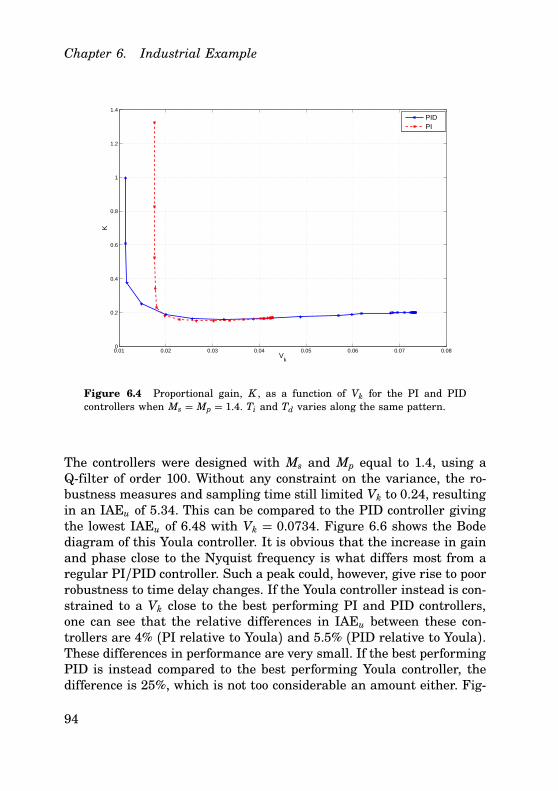
Chapter 6. Industrial Example
0.01 0.02 0.03 0.04 0.05 0.06 0.07 0.080
0.2
0.4
0.6
0.8
1
1.2
1.4
Vk
K
PIDPI
Figure 6.4 Proportional gain, K , as a function of Vk for the PI and PIDcontrollers when Ms = Mp = 1.4. Ti and Td varies along the same pattern.
The controllers were designed with Ms and Mp equal to 1.4, using aQ-filter of order 100. Without any constraint on the variance, the ro-bustness measures and sampling time still limited Vk to 0.24, resultingin an IAEu of 5.34. This can be compared to the PID controller givingthe lowest IAEu of 6.48 with Vk = 0.0734. Figure 6.6 shows the Bodediagram of this Youla controller. It is obvious that the increase in gainand phase close to the Nyquist frequency is what differs most from aregular PI/PID controller. Such a peak could, however, give rise to poorrobustness to time delay changes. If the Youla controller instead is con-strained to a Vk close to the best performing PI and PID controllers,one can see that the relative differences in IAEu between these con-trollers are 4% (PI relative to Youla) and 5.5% (PID relative to Youla).These differences in performance are very small. If the best performingPID is instead compared to the best performing Youla controller, thedifference is 25%, which is not too considerable an amount either. Fig-
94

6.7 Results and conclusions
0 0.02 0.04 0.06 0.08 0.1 0.125
10
15
20
25
30
PID
PI
IAEu
Vk
Figure 6.5 PI and PID controllers for Ms = Mp = 1.2, 1.3 and 1.6
ure 6.7 shows the IAEu plotted against Vk for all Youla parametrizedcontrollers (when Ms = Mp = 1.4) together with the PI/PID curvesthat were already given in Figure 6.2 and 6.5. The conclusion here isthat the process does not benefit much from having a more advancedcontroller.It has been concluded that the high sampling time gives a rather
conservative limit on how well the controllers can perform, given rea-sonable robustness measures.
6.7 Results and conclusions
After the first industrial data had been analyzed, a request was sentto Akzo Nobel to try out the three controllers listed in Table 6.1. PID1is the best performing PID controller for Ms = Mp = 1.4 and PI2 is theequivalent of PI controllers. The reason for selecting the best possiblecontrollers was because the noise is quite insignificant for this process.
95

Chapter 6. Industrial Example
Table 6.1 PI and PID controllers to be evaluated on the real process.
Controller K Ti Td Tf IAEu Est. σ 2u/σ 2nPID1 0.20 1.13 0.26 0.00 6.48 0.073
PI1 0.27 2.34 0.00 1.29 8.77 0.039
PI2 0.17 1.30 0.00 0.00 7.73 0.043
It should thus be alright to push the performance while still keepingthe system robust. PI1 was chosen because of (as described earlier) itsclose relations to a lambda control strategy.About four and a half months after initial data had been collected,
result data arrived. Since the new experiment was conducted so longafter the initial ones, the old model had to be validated with the new
10−2
10−1
100
10−1
100
101
102
Frequency (rad/s)
Mag
nitu
de
10−2
10−1
100
−100
−50
0
50
100
Frequency (rad/s)
Ang
le (
degr
ees)
Figure 6.6 Youla parametrized controller when Ms = Mp = 1.4 and thereis no constraint on the relative variance Vk. Note the phase and magnitudeincrease close to the Nyquist frequency.
96

6.7 Results and conclusions
0 0.025 0.05 0.075 0.1 0.125 0.15 0.175 0.2 0.225 0.255
6
7
8
9
10
11
12
13
14
15
16
1717
Youla ControllerPID ControllerPI Controller
IAEu
Vk
Figure 6.7 Trade-off curves for PI, PID and Youla parametrized controllerswhen Ms = Mp = 1.4.
data to see how significant the process alteration had been. The samehad to be conducted for the noise selection. The filtered process values(solid) and set point (dashed) from the evaluation experiments canbe found in the upper part of Figure 6.8, while the control signal isshown below. The red signals show the time line when the process iscontrolled by the old lambda tuned controller PIλ , however, with thebig difference that T f = 2 instead of 1 (which used to be the case).The reason for this change is not known. The blue curves show stepresponse data, used to verify if the process and measurement noisecharacteristics had changed or not. The black data shows discardedinformation clearly affected by actuator stiction. As stated before, thisproblem is not related to the choice of controller and can thus be ig-nored. The purple data shows the closed loop signals when controlledby PID1. The sharp twist in the middle of the data will, however, notbe part of the analysis. The first sequence of green data correspondsto control using PI1 and the second to PI2 control. When analysing
97

Chapter 6. Industrial Example
0 500 1000 1500 2000 250064
65
66
67
68
69
70
71
72
Time (s)
Mag
nitu
de (
%)
0 500 1000 1500 2000 250059
59.5
60
60.5
61
61.5
62
62.5
63
Time (s)
Mag
nitu
de (
%)
PIλPIλ
PIλ PIλPID1
PID1
PI1
PI1
PI2
PI2
Open loop
Open loop
Figure 6.8 The upper plot shows the filtered process value (solid) and setpoint (dashed) from the industrial verification data, while the lower displaysthe control signal. The three controllers from Table 6.1 was used to evaluate theestimated variances.
the process values, it is important to realize that these are the sig-nals coming in after the low-pass filter. Since PIλ and PI1 both haveactive filters, these signals may look much nicer to the eye than thesequences of the other two controllers. For that reason it would havebeen preferable to have access to raw measurement data instead.First of all, the step response data was used to derive a new model.
Since the old model seemed to be valid for the new data as well, itwas assumed that the process had not changed significantly enough toalter the model. The process noise had changed a little over time, sothat σ 2n = 0.022 instead of 0.026, but that is not a significant changeeither.Earlier, quantization effects have not been considered. Since the
control signal is sometimes quite close to the quantization level inmagnitude (most significantly for PIλ and PI1), however, the effectwas introduced in the evaluation analysis. The quantization level for
98

6.7 Results and conclusions
the control signal is 0.01%.Starting out the analysis with PID1, it is obvious that the control
signal variance is highest for this particular case, just as expected. Thedifference from the other two cases would, however, be rather insignifi-cant if the plot had been zoomed out a bit more. One has to realize thatthe levels of the noise are in magnitude 0.1 − 0.3% of the maximumpossible control signal, which are quite small values. Taking the noisysignal after the sharp switch as data, σ 2u = 0.074 which is 1% off theexpected variance (all estimates were recalculated for the new noise).This is, in other words, a very good match.The two PI controllers have control signal variances σ 2u = 0.0137
for PI1 and 0.0348 for PI2. In the case of PI2, the estimate (0.0432) is24% higher than the real value which seems reasonably close. For PI1,on the other hand, the variance is quite far from the expected value of0.0303 (121% difference). Taking a closer look at the control signal forPIλ shows that its variance is also quite a lot lower than the expectedvalue (about half of it). One possible reason for these differences is thatthe low-pass filter might have the wrong model, which would explainwhy the other two cases, where the filter is inactive, are much closerto the truth. An interesting observation is that setting the filter modelto second order (double pole) actually gives an estimate exactly at thecorrect variance for PIλ . For PI2 the difference is still 85% after chang-ing the filter order, but this do at least give one option of a possibleerror source. It also shows how important it is to have the correct setupfor the actual control system. Even a slight alteration could mean thatthe values end up quite far from the real. For this reason it is highlydesirable that control loops are well documented. This includes the wayin which the controller has been implemented. Just assuming that thelow-pass filter is approximated by forward Euler instead of backwardwould give quite a big variance increase. One way to get around thisissue would be to:
1. Determine the controller that is likely to give the correct variance.
2. If the variance is not the expected, choose either a more or lessaggressive controller on the trade-off curve.
3. Iterate until the control looks satisfactory.
Since the experiments were so short, it is hard to compare the perfor-
99

Chapter 6. Industrial Example
mances of the different controllers. In order to make such a comparison,one would need to have the plant running a long time with the differ-ent controllers active and then compare how the process value variesover time.The experiments on the real plant have shown promising results. It
was not an ideal plant to try the new method on considering samplingrate and stiction effects, but it has given a good indicator that theproposed design method is reasonable. Not all three cases gave varianceclose to the estimated, but then again, all signals were held withinreasonable bounds and none of them blew up in magnitude.The possibly most interesting conclusion one can draw in conjunc-
tion to these industrial experiments is that one can now tune a realPID controller without the fear of having the control signal vary toomuch. One would, however, still need a lot more tests on industrialplants before the method can be fully trusted and utilized.
100

7
When are PI and PID
Controllers Valid Choices?
Previous chapters have shown that PI and PID controllers designed,using the proposed method, may very well be close in performance tothe best possible linear controllers. This was shown by optimization ofYoula parametrized controllers. In this chapter, it will be attemptedto give a bit more general guidelines on when PI and PID controllersare valid choices compared to more advanced control structures. Thework presented here has, however, not yet been in development for verylong and there is thus more to do before any general conclusions canbe drawn. The main goal of this chapter is therefore to inspire futurework rather than presenting the definite answer to when PI and PIDcontrollers should be used.Three sub-batches from the AMIGO test batch (3.1) have been ex-
amined. PI and PID controllers have been compared with Youla con-trollers for several batch processes. In all cases, it has been assumedthat Ms = Mp = 1.4 and that the measurement noise is white, withunit variance, sampled every h = 0.01 seconds. This sampling timewill be treated as the reference sampling time when the up- or down-sampling ratio, J, is derived. That way, one can compare all processesno matter the respective sampling times.It has already been pointed out that the PI and PID controllers de-
rived, using the proposed design method, are not optimal with respectto the variance constraint. To get the full picture of when PI and PIDcontrollers are valid choices, the optimal controllers should ideally be
101

Chapter 7. When are PI and PID Controllers Valid Choices?
used. One way to determine these would be through gridding. This willnot be done here though and one should thus see this chapter mainlyas a way of justifying the proposed design method. It should, however,still be possible to see some trends that are likely to occur even whenthe optimal PI and PID controllers are employed.For the three sub-batches, a limited proportion of the total amount
of processes were analysed. Each process had seven PI controller de-signs and seven PID controller designs - spanning over Tf . The PIcontrollers have, however, not been used much in the analysis here.The Vk-values resulting from the runs were used to design Youla con-trollers giving the same variance to render a comparison possible.
7.1 Sub-batch 1 – First order systems with time delay
The first sub-batch to be investigated is the one with time delayed firstorder systems, that is,
P1(s) =e−s
1+ sT ,
T = 0.1, 0.5, 1, 2, 5, 10, 50, 500,
such that 8 of 21 processes were analysed.Figure 7.1 shows a plot of the relation between IAEPIDu /IAEYoulau
and Vk. In other words, this shows how well the different PID con-trollers perform compared to the Youla controller fulfilling the samevariance constraint. Most of the curves in Figure 7.1 have the sameappearance with a fast growing relative IAEu for low Vk-values, reach-ing stationarity for high Vk-values (see for instance the T = 0.1 case).This seems rather reasonable since the robustness measures will likelydestroy the chances of the Youla controller taking full advantage of itssuperior freedom when Vk is high. For values on T from 5 and above,the curves are shaped such that the relative IAEu decreases for highVk. It does, however, seem logical that the shape of the curve is moreaccurate for low values on T . The reason being that it is reasonableif the PI or PID structure has the highest benefits for low Vk-values,leaving the Youla controller with little freedom. This is also confirmedby looking at the relative IAEu for PI controllers. These have a lot lower
102
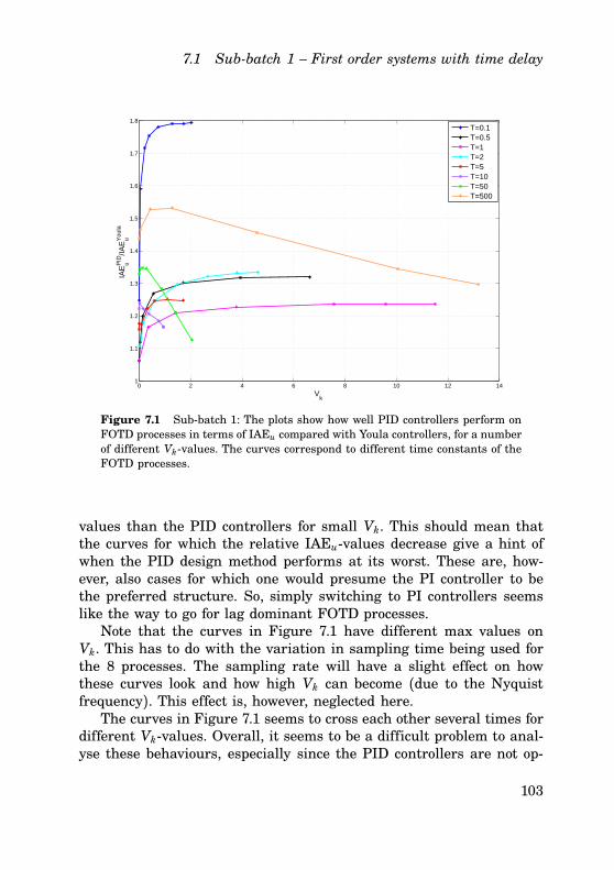
7.1 Sub-batch 1 – First order systems with time delay
0 2 4 6 8 10 12 141
1.1
1.2
1.3
1.4
1.5
1.6
1.7
1.8
Vk
IAE
uPID
/IAE
uYou
la
T=0.1T=0.5T=1T=2T=5T=10T=50T=500
Figure 7.1 Sub-batch 1: The plots show how well PID controllers perform onFOTD processes in terms of IAEu compared with Youla controllers, for a numberof different Vk-values. The curves correspond to different time constants of theFOTD processes.
values than the PID controllers for small Vk. This should mean thatthe curves for which the relative IAEu-values decrease give a hint ofwhen the PID design method performs at its worst. These are, how-ever, also cases for which one would presume the PI controller to bethe preferred structure. So, simply switching to PI controllers seemslike the way to go for lag dominant FOTD processes.Note that the curves in Figure 7.1 have different max values on
Vk. This has to do with the variation in sampling time being used forthe 8 processes. The sampling rate will have a slight effect on howthese curves look and how high Vk can become (due to the Nyquistfrequency). This effect is, however, neglected here.The curves in Figure 7.1 seems to cross each other several times for
different Vk-values. Overall, it seems to be a difficult problem to anal-yse these behaviours, especially since the PID controllers are not op-
103

Chapter 7. When are PI and PID Controllers Valid Choices?
0 0.1 0.2 0.3 0.4 0.5 0.6 0.7 0.8 0.9 11.1
1.2
1.3
1.4
1.5
1.6
1.7
1.8
τ
IAE
uPID
/IAE
uYou
la
Figure 7.2 Sub-batch 1: Relative IAEu-values for maximal Vk from the curvesin Figure 7.1. These shows a trend that more complex controllers have a biggeradvantage for delay dominant FOTD processes.
timal, in contradiction to the Youla controllers. Small variations couldtherefore be due to this imperfection rather than real differences be-tween the processes. The stationary values (high Vk) in all cases, ex-cept T = 500, were compared. These values, that are plotted in Figure7.2, gives a measure of when a PID controller is close in performanceto a Youla controller. The benefits from using the advanced controllerstructure are very small for low values on the normalized time delay,τ . This is quite reasonable since these systems are basically first or-der systems with negligible time delay. When the time delay is thedominant part of the system, however, the Youla controller shines themost. These controllers will typically include a lot of peaks though,thus ruining robustness towards time delay changes. Also note thatthere is a dip in the curve, shown in Figure 7.2, for τ ( 0.5 and apeak when τ ( 0.3. It would have been logical to assume that thiscurve is monotonically increasing with τ , with the motivation that the
104

7.2 Sub-batch 2 – Second order systems with time delay
time delay makes the system harder to control. The time delay robust-ness will, however, sabotage this relation and one would really needto derive a good time delay compensating controller with sufficient ro-bustness to really get a good picture of whether the advanced structureis important for τ ( 1 or not. A guess is that the curve, taking delayrobustness into consideration would have rather low values for bothτ & 0 and τ . 1. Such that there would be some maximum in betweenwhen the advanced controller is preferred the most compared to a PIor PID controller. Whether or not this is actually the case, it still seemslike the FOTD systems are gaining relatively little from using the ad-vanced structure of the Youla controller. The PI and PID controllersseem to be valid choices to use for these systems. PI for low Vk and τclose to 0 and possibly also close to 1. PID for higher values on Vk andwhen the system is somewhere in between lag- and delay dominant.As a complement to the analysis above, consider the case when
the variance of the control signal can not be higher than that of themeasurement noise, that is when Vk = 1. Figure 7.3 and 7.4 shows theYoula and PID controllers respectively for 5 of the 8 different sub-batchprocesses. Looking at the Youla controllers show how they graduallybecome less and less complex as T increases. The same is true for thePID controllers that start out with a distinct D-part, but ends witha roughly filtered controller when T = 500. Figure 7.5 confirms thisobservation, showing how the relation T f /Td increases with decreasingτ for the PID controllers, thus basically giving PI controllers in the end.
7.2 Sub-batch 2 – Second order systems with time delay
Next in line of analysis is the second sub-batch, containing second ordersystems with time delay
P2(s) =e−s
(1+ sT)2 ,
T = 0.1, 0.5, 1.5, 6, 20, 200,
such that 6 of 21 processes were analysed. These processes span frombeing delay dominant when T = 0.1 to become lag dominant, essen-tially of order two with negligible dead time, when T is high.
105

Chapter 7. When are PI and PID Controllers Valid Choices?
10−3
10−2
10−1
100
101
100
101
102
103
Frequency (rad/s)
Mag
nitu
de
T=0.5T=2T=10T=50T=500
Figure 7.3 Sub-batch 1: Youla parametrized controllers for 5 different FOTDprocesses, given that Vk = 1. Advanced controllers are preferred when the sys-tem is delay dominant, while lower order controllers are preferred for lag dom-inant processes.
10−3
10−2
10−1
100
101
100
101
102
103
Frequency (rad/s)
Mag
nitu
de
T=0.5T=2T=10T=50T=500
Figure 7.4 Sub-batch 1: PID controllers for 5 different FOTD processes, giventhat Vk = 1.
106

7.2 Sub-batch 2 – Second order systems with time delay
0 0.1 0.2 0.3 0.4 0.5 0.6 0.7 0.8 0.9 10
0.2
0.4
0.6
0.8
1
1.2
1.4
1.6
1.8
τ
Tf/T
d
Figure 7.5 Sub-batch 1: The relation between T f /Td and τ , when Vk = 1shows that the D-part of the PID controller is the most useful for processes thatare not lag dominant.
Figure 7.6 shows once again how IAEPIDu /IAEYoulau changes depend-ing on process dynamics and the limit of control signal variance, i.e.Vk. The patterns are quite similar to those plotted in Figure 7.1, sug-gesting that the proposed design method is furthest from optimalityfor lag dominant systems with small Vk-values.Plotting the values for which Vk is the highest, gives the curve in
Figure 7.7. This plot is also very similar to the sub-batch 1 equivalentin Figure 7.2, but sub-batch 2 seems a little bit harder to control forequivalent numbers on τ . The possibly most interesting bit is that thecurve dips at τ ( 0.5 just like before. Whether or not this is an effectcaused by the proposed method alone remains an open question forfuture work.Fixating Vk to 1 gives the Youla controllers shown in Figure 7.8. The
controllers for the delay dominant systems remind a lot of those fromsub-batch 1. As τ decreases, the controllers do not seem to become sim-
107

Chapter 7. When are PI and PID Controllers Valid Choices?
0 2 4 6 8 10 121
1.1
1.2
1.3
1.4
1.5
1.6
Vk
IAE
uPID
/IAE
uYou
la
T=0.1T=0.5T=1.5T=6T=20T=200
Figure 7.6 Sub-Batch 2: These plots show how well PID controllers performon second order processes with time delay in terms of IAEu compared withYoula controllers, for a number of different Vk-values. The curves correspond todifferent time constants of the processes.
ilar to PI controllers which was the case for the FOTD systems. Thatis also quite logical since a second order process without time delayis known to be controlled sufficiently well with a PID controller. A PIcontroller will, however, lack freedom to set the closed loop dynamics.Unless of course one puts really high demands on the control signalvariance, thus gimping the potential of the more advanced controllers.Plotting T f/Td versus τ , when Vk = 1, confirms that the D-part
is more important for the second order processes with dead-time com-pared to the FOTD systems. The T f /Td values are much smaller thanbefore. An interesting detail is that the relation has a maximum aroundτ = 0.2 and decreases for lower values on τ . If this is an indicator ofbad controllers or a real feature of these systems remains to be shown.
108

7.3 Sub-batch 9 – Systems with complex poles
0.1 0.2 0.3 0.4 0.5 0.6 0.7 0.8 0.91.15
1.2
1.25
1.3
1.35
1.4
1.45
1.5
1.55
1.6
τ
IAE
uPID
/IAE
uYou
la
Figure 7.7 Sub-batch 2: Plot that shows the relative IAEu-values for maximalVk from the curves in Figure 7.6. Just as in the case of sub-batch 1, the trendis that more complex controllers have a bigger advantage for delay dominantFOTD processes.
7.3 Sub-batch 9 – Systems with complex poles
The third and last sub-batch to be analysed is
P1(s) =1
(s+ 1)((sT)2 + 1.4sT + 1) ,
T = 0.1, 0.4, 1,
which consists of processes with one real pole and two complex conju-gated poles. When T = 1, these poles are at the same distance from ori-gin, while the two complex poles are quite insignificant when T = 0.1.The system will thus span from basically being a first order systemto become a third order process. Looking at the relative IAE differ-ences between the PID and Youla controllers show (see Figure 7.10)that there are more significant differences in performance compared
109

Chapter 7. When are PI and PID Controllers Valid Choices?
10−3
10−2
10−1
100
101
100
101
102
103
Frequency (rad/s)
Mag
nitu
de
T=0.1
T=0.5
T=1.5
T=6
T=20
T=200
Figure 7.8 Sub-batch 2: Bode magnitude plots of the Youla controllers whenVk = 1.
to the previous sub-batches. The τ -values will span a much smallerregion than for earlier batches, with: τ = 0.12 when T = 0.1, τ = 0.26for T = 0.4 and τ = 0.31 with T = 1. It is obvious that the Youlacontroller is superior when there are three significant poles and Vk isset high. The process with T = 0.1 can, however, be controlled quitewell with the PID controller although the shape of the curve suggeststhat the given controllers are not quite optimal.Taking the case when Vk = 1 shows once again that the more
delay dominant system (here T = 1) have more use for an advancedcontroller than the lag dominant systems. This is shown in Figure7.11. Also note that these controllers will give good robustness to timedelay variations (no high peaks), so the Youla controllers will, withoutdoubt, be a lot better than PID controllers in this case. It should alsobe fine to reduce these controllers to receive ones that are really closeto optimal.
110

7.4 Summary
0.1 0.2 0.3 0.4 0.5 0.6 0.7 0.8 0.90.04
0.06
0.08
0.1
0.12
0.14
0.16
0.18
τ
Tf/T
d
Figure 7.9 Sub-batch 2: The relation between T f /Td and the normalized timedelay when Vk = 1. The D-part is more significant than for the processes in sub-batch 1.
The Tf /Td versus τ relation, for the PID controllers when Vk = 1,is strictly decreasing in this case. For T = 1 one gets T f/Td = 0.17,while T = 0.4 lead to Tf /Td = 0.19 and T = 0.1 to T f/Td = 0.37. Thisis, however, just as expected. The process that is the closest to a firstorder system being the process that needs the D-part the least.
7.4 Summary
Looking through the different plots presented in this chapter, it is obvi-ous that whether or not a PI or PID controller is sufficient will dependon both the process dynamics and the allowed control signal activity. Ifthe control signal variance due to measurement noise is allowed to belarge, then the freedom of an advanced controller will come to its rightto a higher degree. If the system is simple, however, it will generally
111

Chapter 7. When are PI and PID Controllers Valid Choices?
0 10 20 30 40 50 601
1.2
1.4
1.6
1.8
2
2.2
Vk
IAE
PID
/IAE
You
la
T=0.1
T=0.4
T=1
Figure 7.10 Sub-Batch 9: The plots show how well PID controllers performon third order processes, with complex poles, in terms of IAEu compared withYoula controllers, for a number of different Vk-values.
not be any point in using the advanced controller and a PID or evenPI is close to optimum. If the process is delay dominant, the advancedcontrollers may seem to give really good results too, but one will thenhave to take into account that the given optimization problem does nothandle robustness towards time delay changes. Such robustness mea-sures could potentially mean that the most delay dominant processesshould really be controlled by simple controllers too.As stated in the beginning of this chapter, these results were de-
rived in the end of the making of this thesis. The results should be seenas a source of inspiration for future work rather than a presentationof the absolute truth. In order to get the full picture, one would reallyneed to derive the PI and PID controllers that are optimal with respectto the variance constraint. The results derived here should, however,at least be representative for the proposed design method.
112

7.4 Summary
10−2
10−1
100
101
100
101
102
Frequency (rad/s)
Mag
nitu
de
Youla, T=0.1PID, T=0.1Youla, T=0.5PID, T=0.5Youla, T=1PID, T=1
Figure 7.11 Sub-Batch 9: Bode magnitude plots for the Youla and PID con-trollers when Vk is fixated to 1. The PID controller is the most similar to theYoula controller when T = 0.1, i.e. when the process is essentially a first ordersystem.
113

8
Conclusions and Future
Work
The following chapter will give a brief summary of the most importantcontributions of the thesis and present some suggestions for futurework within the research area.
8.1 Conclusions
Many industrial processes have relatively simple dynamics, that aregenerally easy to control with PI or PID controllers. Even so, the sheernumber of control loops makes it a very time-consuming duty to tuneall of them. Lack of time and knowledge among operators will thusoften leave controllers with default settings, far from optimal. For thisreason it is important to have a controller design tool that is bothfast and easy to use. While there are many design methods alreadysatisfying this, few guarantee to fulfill all of the following three closedloop criterias:
• Fast load disturbance suppression
• Closed loop robustness to model errors and process variations
• Low actuator wear and tear
While the third criteria is seldom an issue with PI control, it is ex-tremely important when designing PID controllers. Control signal sen-sitivity to measurement noise is one of the most important reasons why
114

8.1 Conclusions
the D-part is seldomly used in industry today. It is simply too costlyto exchange actuators in relation to the performance gain one getsthrough using the D-part. Add to this that tuning three, or even four,controller parameters is far more complicated than just two and it isnot difficult to understand the decision.The PID design method proposed within this thesis takes all three
of the above stated criterias into consideration. The controllers are op-timized through a fast and robust Matlab software tool such that theIAE-value during a load disturbance is minimized, with respect to ro-bustness constraints on the sensitivity- and complementary sensitivityfunction. The tool can then be run several times for different settingson the low-pass filter, through which the measurements have to pass.Estimating the control signal variance due to measurement noise willprovide the user with a trade-off curve between performance and con-trol signal activity. This way, the wear on actuators can be taken intoconsideration when designing the controllers. Furthermore, the designtool can be used to choose a PI or PID controller depending on whichis the best suited for the given process. This will be a decision that istaken both with respect to the process and the allowed control signalactivity.It is a good idea to check the quality of the controllers since the
proposed software design tool give optimal controllers with respect torobustness, but not to the control activity constraint. In order to doso, optimized Youla parametrized controllers were used. These give agood estimate of how close the designed PI and PID controllers are tothe limit of performance. A small difference in performance is a verygood sign that the simple controllers are well-tuned. Several examplesprovided within this thesis have also shown that this is very often true.In the cases that PID controllers are less suitable, it is often advisableto switch to PI control. This is also supported by the observation thatthe Youla controllers are basically PI controllers in these cases. Thereare of course other types of processes, like oscillatory systems, whenPID control is known to give rather poor results. In such cases, it seemsadvisable to use more advanced controllers. One way of doing so couldbe to start out from the Youla controllers and proceed through somecontroller reduction method. It is, however, important that extra timespent on deriving more advanced controllers is really worth it, or elsea simpler controller may very well be better to use.
115

Chapter 8. Conclusions and Future Work
Several experiments on real processes have shown that the proposeddesign method has good potential to work well in industry. It is possibleto estimate the control signal variance due to measurement noise andkeep it as low as specified, which opens up for use of PID controllersin industry.
8.2 Future work
During the work of this thesis, several questions have come up thatwill need further attention in the future. Here follows a few of them:
• How can one extend the controller design to include fully autom-atized estimation of the control signal variance and plotting ofthe trade-off curve?
• Is it possible to use Youla controllers to systematically tune evenbetter controllers whose level of complexity depends on the pro-cess dynamics and allowed control signal activity?
• The proposed controller design tool should ideally be able tochoose optimal controller structure depending on the process. Isthis possible to achieve?
In addition to these questions, it should be reminded that the is-sues presented in Chapter 7 are not yet fully investigated. More workis needed before it is possible to give any general guidelines on whenPI and PID controllers are valid choices compared to more advancedoptions. Furthermore, the PI and PID controllers used in the compar-isons should ideally be optimal with respect to the variance constraint.This could for instance be achieved through gridding.Experiments on an industrial process has already been conducted,
but several more tests are needed before the proposed design methodcan be utilized with full confidence.There are also several nearby areas like event-based PID control
and control of two-inputs-two-outputs systems that could possibly betreated similarly to the methods described in this thesis. Whether ornot these ideas have potential will also be left for future work to show.
116

9
Bibliography
Åkesson, J. (2008): “Optimica—An Extension of Modelica SupportingDynamic Optimization.” In 6th International Modelica Conference2008. Modelica Association.
Årzén, K.-E. (1996): Real-Time Control Systems. Department of Auto-matic Control, Lund Institute of Technology, Lund, Sweden.
Åström, K. J. and T. Hägglund (2001): “The future of PID control.”Control Engineering Practice, 9, pp. 1163–1175.
Åström, K. J. and T. Hägglund (2005): Advanced PID Control. ISA -The Instrumentation, Systems, and Automation Society, ResearchTriangle Park, NC 27709.
Åström, K. J. and B. Wittenmark (1997): Computer ControlledSystems—Theory and Design. Prentice Hall, Upper Saddle River,New Jersey.
Boyd, S., C. Barratt, and S. Norman (1990): “Linear Controller Design:Limits of Performance Via Convex Optimization.” Proceedings ofthe IEEE, 78:6, pp. 529–574.
Boyd, S. P. and C. Barratt (1992): “Closed-loop Convex Analysisof Performance Limits for Linear Control Systems.” In IEEESymposium on Computer Aided Control System Design, pp. 301–304. Napa, California, USA.
Boyd, S. P. and C. H. Barratt (1991): Linear Controller Design—Limitsof Performance. Prentice Hall, Englewood Cliffs, New Jersey.
117

Chapter 9. Bibliography
Buckbee, G. (2002): “Poor Controller Tuning Drives Up Valve Costs.”Control Magazine, April.
Dahlin, E. B. (1968): “Designing and tuning digital controllers.”Instruments and Control Systems, 42, June, pp. 77–83.
Garpinger, O. and T. Hägglund (2008): “A Software Tool for RobustPID Design.” In IFAC World Conference. Seoul, South Korea.
Hägglund, T. and K. J. Åström (1991): “Industrial adaptive controllersbased on frequency response techniques.” Automatica, 27, pp. 599–609.
Hägglund, T. and K. J. Åström (2004): “Revisiting the Ziegler-Nicholsstep response method for PID control.” Journal of Process Control,14:6, pp. 635–650.
Isaksson, A. J. and S. F. Graebe (2002): “Derivative filter is anintegral part of PID design.” Control Theory and Applications, IEEProceedings, 149, January, pp. 41–45.
Kristiansson, B. and B. Lennartson (2006): “Evaluation and simpletuning of PID controllers with high-frequency robustness.” Journalof Process Control, 16, pp. 91–102.
Lagarias, J. C., J. A. Reeds, M. H. Wright, and P. E. Wright (1998):“Convergence properties of the Nelder-Mead simplex algorithm inlow dimensions.” SIAM Journal on Optimization, 9, pp. 112–147.
Li, Y., K. H. Ang, and G. C. Y. Chong (2006): “PID control systemanalysis and design - Problems, remedies, and future directions.”IEEE Control Systems Magazine, 26, pp. 32–41.
Luyben, W. L. (2001): “Effect of derivative algorithm and tuningselection on the PID control of dead-time processes.” Ind. Eng.Chem. Res., 40, pp. 3605–3611.
Marlin, T. E. (1995): Process Control. Designing Processes and ControlSystems for Dynamic Processes. McGraw-Hill.
Nelder, J. A. and R. Mead (1965): “A simplex method for functionminimization.” Computer Journal, 7, pp. 308–313.
118
Nordfeldt, P. (2005): “PID Control of TITO Systems.” LicentiateThesis ISRN LUTFD2/TFRT--3238--SE. Department of AutomaticControl, Lund University, Sweden.
Norman, S. A. and S. P. Boyd (1989): “Numerical solution of a two-disk problem.” In American Control Conference, pp. 1745–1747.Pittsburgh.
Olsen, T. and B. Bialkowski (2002): “Lambda Tuning as a PromisingController Tuning Method for the Refinery.” In 2002 AIChE SpringNational Meeting. New Orleans, USA.
Oviedo, J. J. E., T. Boelen, and P. van Overschee (2006): “Robustadvanced PID control (RaPID) - PID tuning based on engineeringspecifications.” IEEE Control Systems Magazine, 26, pp. 15–19.
Panagopoulos, H., K. J. Åström, and T. Hägglund (2002): “Design ofPID controllers based on constrained optimisation.” IEE Proceed-ings - Control Theory & Applications, 149:1, pp. 32–40.
Wallén, A. (2000): Tools for Autonomous Process Control. PhD thesisISRN LUTFD2/TFRT--1058--SE, Department of Automatic Con-trol, Lund Institute of Technology, Sweden.
Walters, F. H., L. R. Parker Jr, S. L. Morgan, and S. N. Deming (1991):Sequential Simplex Optimization. CRC Press LLC.
Wernrud, A. (2008): QTool 0.1—Reference Manual. Department ofAutomatic Control, Lund University, Lund, Sweden.
119


Department of Automatic Control
Lund UniversityBox 118
SE-221 00 Lund Sweden
Document nameLICENTIATE THESISDate of issueMarch 2009Document NumberISRN LUTFD2/TFRT--3245--SE
Author(s)Olof Garpinger
Supervisor
Tore Hägglund
Sponsoring organisation
Swedish Research Council (VR)Title and subtitle
Design of Robust PID Controllers with Constrained Control Signal Activity
Abstract
This thesis presents a new method for design of PI and PID controllers with the level of control signalactivity taken into consideration. The main reason why the D-part is often disabled in industrial controlloops is because it leads to control signal sensitivity of measurement noise. A frequently varying controlsignal with too high amplitude will very likely lead to actuator wear and tear. For this reason it isextremely important for any PID design method to take this into account.
The proposed controllers are derived using a newly developed design software that solves an IAE min-imization problem with respect to H∞ robustness constraints on the sensitivity- and complementarysensitivity function. The software is shown to be fast, easy to use and robust in giving well-performingcontrollers.
By extracting measurement noise from the process value of a real plant, one can estimate its effect onthe control signal variance. The time constant of the low-pass filter, through which measurements arefed, is varied to design controllers with constrained control signal activity. By comparing control signalvariance and IAE, the user is also able to weigh actuator wear to estimated performance.
The proposed PID design method has shown to give very promising results both on simulated examplesand real plants such as a recirculation flow process.
Optimal Youla parametrized controllers are used both as a quality check of the designed PI and PIDcontrollers and as a tool for determining when these are valid choices compared to more advanced con-trollers.
Key wordsPID control, process control, disturbance rejection, linear systems, constrained control signal activity,measurement noise, algorithms and software, Youla parameterized controllers
Classification system and/or index terms (if any)
Supplementary bibliographical information
ISSN and key title
0280–5316ISBN
Language
EnglishNumber of pages
122Security classification
Recipient’s notes
The report may be ordered from the Department of Automatic Control or borrowed through:University Library, Box 134, SE-221 00 Lund, SwedenFax +46 46 222 42 43 E-mail [email protected]