Electronic copy available at: http://ssrn.com/abstract=1493227

Conflicting Tasks and Moral Hazard: Theory andExperimental Evidence∗

Eva I. Hoppe and David J. Kusterer

University of Cologne, Germany

Abstract

We study a multi-task principal-agent problem in which tasks can be in direct

conflict with each other. In theory, it is difficult to induce a single agent to

exert efforts in two conflicting tasks, because effort in one task decreases the

success probability of the other task. We have conducted an experiment in

which we find strong support for the relevance of this incentive problem. In

the presence of conflict, subjects choose two high efforts significantly less often

when both tasks are assigned to a single agent than when there are two agents

each in charge of one task.

Keywords: moral hazard; conflicting tasks; experiment

JEL Classification: D86; C90; M54

∗ Department of Economics, University of Cologne, Albertus-Magnus-Platz, 50923 Köln,

Germany. E-mail: <eva.hoppe@uni-koeln.de> and <david.kusterer@uni-koeln.de>. We

would like to thank Patrick Schmitz for very helpful and inspiring discussions at any time

and for critical comments that have significantly improved the paper.

1

Electronic copy available at: http://ssrn.com/abstract=1493227

1 Introduction

In real-world agency problems, it is often the case that principals have to

delegate not just one but several tasks. In this paper we focus on situations in

which two different tasks to be delegated may be in direct conflict with each

other; i.e., providing effort in one task may have a negative side effect on the

success probability of the other task. In such situations, job design becomes a

major issue. In particular, it might be the case that implementing high effort

in both tasks may be facilitated by hiring two different agents each in charge

of one task instead of letting one agent be responsible for both tasks. In the

present paper we investigate these incentive problems in a theoretical model

and provide first experimental evidence that agents are indeed reluctant to

perform different tasks when they are in conflict with each other.

To fix ideas, consider a merchant (principal) who wants to sell two products

which may be imperfect substitutes. The merchant may hire either one or two

sales representatives (agents) who can exert effort to promote the products.

The effort decisions are assumed to be non-contractible, but the wages can

depend on which products are sold. The agents are risk-neutral and have no

wealth, so that the wages must be non-negative. There are no technological

(dis)economies of scope, so that in the absence of incentive problems, the

principal would be indifferent between hiring one or two agents.

Suppose first that the merchant has only one sales representative in charge

of both products. If the products are imperfect substitutes, then promotion

effort in one task increases the probability of sale of the promoted product,

but at the same time it lowers the probability of sale of the other product (i.e.,

there is conflict between the tasks). In contrast, if there is no relation between

the products, promotion of one product has no effect on the probability of sale

of the other product. We consider a symmetric situation such that in theory,

when the products are unrelated (so that there is no conflict), the principal

induces either high effort in both tasks or no high effort at all. However, when

there is conflict between the tasks, then it may be optimal for the principal

to induce the agent to invest effort in only one task. Intuitively, if there is

conflict between the two tasks, a single sales representative is very reluctant

to exert effort in both tasks, because he knows that promotion effort does not

only increase the probability of sale of the promoted product, but at the same

time it also lowers the probability of sale of the other product he is supposed to

2

sell. This makes it very expensive for the principal to induce two high efforts.

Suppose next that there are two (identical) sales representatives, each of

them responsible for promoting one product. Due to symmetry, in theory

the principal induces either high effort in both tasks or no high effort at all,

regardless of whether or not there is conflict.

In general, if there is conflict, it depends on the parameter constellation

whether the principal’s expected profit is larger with one or with two agents.

Yet, if there is no conflict, then the principal’s expected profit is unambiguously

larger when only one agent is in charge of both tasks. Intuitively, when the

tasks are not in conflict with each other, the rent that the principal leaves to

the agent to motivate him to work on one task can also be used to motivate

him to work on the other task.

In order to assess whether the theoretical problem of inducing a single agent

to exert efforts in conflicting tasks may be empirically relevant, we conducted a

laboratory experiment with 474 subjects. There are two treatments with con-

flict; one where the principal has only a single agent and another one where

she has two agents. We have chosen a parameter constellation such that ac-

cording to standard theory, a merchant who has only one sales representative

would induce him to invest effort in only one task, while a merchant with two

sales representatives would induce each one to promote his respective product.

Moreover, there are two treatments without conflict, one with a single agent

and another one with two agents. The theoretical prediction for our parame-

ter constellation is that in the absence of conflict, a merchant would always

induce two high efforts, regardless of whether she has only one or two sales

representatives to perform these tasks.

The main experimental findings are largely in line with these predictions,

even though the principals made more generous wage offers, which is not sur-

prising given previous experimental evidence. In particular, our central result

is that in the one-agent treatment with conflict, two high efforts are observed

significantly less often than in the other three treatments. In the one-agent

treatment with conflict, the theoretically predicted expected profit of the prin-

cipal is only slightly smaller than in the two-agent treatment with conflict.

In the experiment, we find no statistically significant difference between the

principals’ profits in these two treatments. Yet, with regard to the no-conflict

treatments, we find that the principals’ profits are significantly larger in the

case of one agent than in the case of two agents, which is in accordance with

3

the theoretical prediction.

Since the seminal work of Holmström and Milgrom (1991), multi-task

principal-agent problems have played a prominent role in the contract the-

oretic literature.1 However, most of these papers have focused on effort sub-

stitution and the trade-off between insurance and incentives when agents are

risk-averse. More recently, many authors have studied moral hazard models

with risk-neutral but wealth-constrained agents.2 In the latter framework,

several authors have shown that a principal can save agency costs if she lets

one agent be in charge of several tasks (see e.g. Hirao, 1993, Che and Yoo,

2001, Laux, 2001, and Mylovanov and Schmitz, 2008).3 The potential bene-

fits of separating tasks in sequential agency problems have been discussed by

Hirao (1993), Schmitz (2005), Khalil, Kim, and Shin (2006). The fact that

conflicts between different tasks may explain why they are delegated to dif-

ferent agents (“advocates”) has first been studied by Dewatripont and Tirole

(1999). They analyze the optimality of organizing the judicial system in an

incomplete contracting framework. The present paper is most closely related

to a complete contracting variant of their model which is discussed in Bolton

and Dewatripont (2005, Section 6.2.2). To the best of our knowledge, only a

few experiments on multi-task principal-agent problems have been conducted

so far. In particular, Fehr and Schmidt (2004) study a problem where one task

is contractible and focus on pros and cons of piece rate versus bonus contracts.

Brüggen and Moers (2007) investigate the role of financial and social incen-

tives in multi-task settings where agents choose an effort level and an effort

allocation.

The remainder of the paper is organized as follows. The theoretical model

which is based on Bolton and Dewatripont (2005) is analyzed in Section 2

and serves as a motivation for our experimental study. The experimental

design is introduced in Section 3 and qualitative hypotheses are derived in

Section 4. The experimental results are presented and discussed in Section 5.

Finally, concluding remarks follow in Section 6. All proofs are relegated to the

appendix.

1For surveys, see e.g. Dewatripont, Jewitt, and Tirole (2000), Laffont and Martimort

(2002, ch. 5), and Bolton and Dewatripont (2005, ch. 6).2See e.g. Innes (1990), Park (1995), Kim (1997), Pitchford (1998), and Tirole (2001).3See also Baron and Besanko (1992), Dana (1993), and Gilbert and Riordan (1995), who

have found related results in other frameworks.

4

2 The theoretical framework

Consider a principal who wants to sell a single unit of a product 1 and a single

unit of a product 2. The sales level for a given product i ∈ {1, 2} is denoted byqi ∈ {0, 1} . If product i is sold, the principal obtains revenue R. We considertwo different scenarios. In the first scenario the principal employs a single agent

to sell product 1 and 2, while she employs two agents in the other scenario.

All parties are risk-neutral. An agent has no wealth and his reservation utility

is zero. If there is only a single agent he can exert effort ai ∈ {0, 1} to promoteproduct i ∈ {1, 2} . In case that there are two agents, agent A can promoteproduct 1 and agent B can promote product 2; i.e., A chooses a1 ∈ {0, 1} andB chooses a2 ∈ {0, 1} . The effort levels are non-contractible.Effort to promote product i increases the probability of sale of product i

but (weakly) lowers the probability of sale of product j 6= i. In other words,

there may be a direct conflict between the effort tasks when the products

are imperfect substitutes. Formally, let the probability of sale of product i

be given by Pr(qi = 1) = α + ρai − γaj. The base rate of sale of product i

is α > 0. If product i is promoted (i.e., ai = 1), the probability of sale of

product i increases by ρ > 0. If the other product j 6= i is promoted (i.e.,

aj = 1) and the products are imperfect substitutes, the probability of sale of

product i decreases by γ > 0. When the products are unrelated (γ = 0), effort

to promote one product has no effect on the probability of sale of the other

product.

Throughout we assume that γ ≤ α ≤ 1−ρ to ensure that 0 ≤ α+ρai−γaj ≤1 for any combinations of effort decisions a1 and a2. An agent has to incur effort

costs ψ if he promotes a product i. Hence, product i generates an expected

net surplus of (α + ρai − γaj)R − aiψ. Due to the symmetry of the model it

is either efficient to promote both or no products. We assume ρ > γ such

that (α + ρ − γ)R− ψ > αR which implies that it is efficient to promote

both products (i.e., a1 = a2 = 1). To induce an agent to exert effort the

principal can offer a wage scheme wq1q2 : = w(q1, q2) that is contingent on

which products have been sold.

One-agent scenario

Given that the principal has only one agent, she has to decide whether to

induce promotion effort in both tasks, in only one task, or in no task.

Let us first consider the case where the principal wishes to induce high

5

effort in both tasks. The principal’s problem is to minimize the expected

compensation E [wq1q2 | a1 = a2 = 1] she has to pay to her agent subject to

the constraints wq1q2 ≥ 0,

E [wq1q2 | a1 = a2 = 1]− 2ψ ≥ E [wq1q2 | a1 = 1, a2 = 0]− ψ, (IC 1)

E [wq1q2 | a1 = a2 = 1]− 2ψ ≥ E [wq1q2 | a1 = 0, a2 = 1]− ψ, (IC 2)

E [wq1q2 | a1 = a2 = 1]− 2ψ ≥ E [wq1q2 | a1 = a2 = 0] , (IC 3)

E [wq1q2 | a1 = a2 = 1]− 2ψ ≥ 0. (PC)

The first two incentive compatibility constraints ensure that the agent

prefers exerting two efforts to exerting only one effort and the third one en-

sures that the agent prefers exerting two efforts to exerting no effort. The last

constraint ensures that the agent participates.

Lemma 1 Suppose the principal wants to induce a1 = a2 = 1. Then she sets

w11 =2ψ

(α+ρ−γ)2−α2 and w10 = w01 = w00 = 0. Given this wage, scheme the

principal’s expected profit is Πhh = (α+ ρ− γ)2(2R−w11) + 2(α+ ρ− γ)(1−α− ρ+ γ)R.

Suppose next the principal wants to induce high effort in only one task. Let

us assume w.l.o.g. that the principal wants to induce high effort with regard

to product 1; i.e., the principal wishes to implement a1 = 1, a2 = 0. In this

case the principal’s problem is to minimize E [wq1q2 | a1 = 1, a2 = 0] subject tothe constraints wq1q2 ≥ 0,

E [wq1q2 | a1 = 1, a2 = 0]− ψ ≥ E [wq1q2 | a1 = a2 = 1]− 2ψ, (IC 1)

E [wq1q2 | a1 = 1, a2 = 0]− ψ ≥ E [wq1q2 | a1 = 0, a2 = 1]− ψ, (IC 2)

E [wq1q2 | a1 = 1, a2 = 0]− ψ ≥ E [wq1q2 | a1 = a2 = 0] , (IC 3)

E [wq1q2 | a1 = 1, a2 = 0]− ψ ≥ 0. (PC)

Lemma 2 Suppose the principal wants to induce a1 = 1 and a2 = 0.4 Then

it is optimal for her to set w10 =ψ

αγ+ρ(1−α+γ) and w11 = w01 = w00 = 0. Given

this wage scheme, the principal’s expected profit is Πhl = (α+ ρ)(α− γ)2R +

(α+ ρ)(1− α+ γ)(R− w10) + (1− α− ρ)(α− γ)R.

4Note that due to the symmetry of the problem the principal’s expected profit is the

same if she implements a1 = 0 and a2 = 1.

6

Observe that if there is conflict and the principal wants the agent to pro-

mote product 1 only, then it is strictly optimal to pay the agent no wage in

case that also product 2 is sold. The reason is that effort in task 1 reduces the

probability of sale of product 2 and hence the sale of this product can be seen

as a signal that the agent may not have promoted product 1. In contrast, if

there is no conflict, a wage scheme with w11 = 0 is not the only solution. This

is because then the sale of product 2 provides no signal for the effort level in

task 1. Therefore, a positive wage w11 can be optimal as long as it does not

induce the agent to promote product 2 as well. Specifically, it is easy to show

that if γ = 0, then any wage scheme 0 ≤ w11 ≤ 1+ρρ(α+ρ)

ψ,w10 ≥ 0, w01 = w00 = 0

which satisfies αw11 + (1− α)w10 =ψρis optimal.

Finally the principal could induce no effort at all. It is immediate to see that

for this case the optimal wage scheme is simply w11 = w10 = w01 = w00 = 0.

Then the principal’s expected profit is Πll = 2αR.

The preceding discussion immediately implies the following result.

Proposition 1 (i) If R > ψ(α+ρ−γ)2[(α+ρ−γ)2−α2](ρ−γ) and R > 2ψ(α+ρ−γ)2

[(α+ρ−γ)2−α2](ρ−γ) −(α+ρ)(1−α+γ)ψ

[αγ+ρ(1−α+γ)](ρ−γ) , then the principal induces high effort in both tasks.

(ii) If (α+ρ)(1−α+γ)ψ[αγ+ρ(1−α+γ)](ρ−γ) < R < 2ψ(α+ρ−γ)2

[(α+ρ−γ)2−α2](ρ−γ) −(α+ρ)(1−α+γ)ψ

[αγ+ρ(1−α+γ)](ρ−γ) , then

the principal induces high effort in only one task.

(iii) Otherwise the principal induces no effort.

It is obvious that the principal will induce promotion for both products if

the return is sufficiently large. However for intermediate values of R, if there is

conflict, the principal may prefer to induce effort in only one task. The reason

is as follows. If the adverse effects of promotion efforts increase, the sale of

two products provides weaker evidence that the agent has chosen high efforts

in both tasks, while the sale of only one product provides stronger evidence

that the agent has exerted high effort to promote this product. As a conse-

quence, if the conflict between tasks increases, it becomes more expensive for

the principal to induce the agent to promote both products, while it becomes

less expensive to implement effort in only one task.

In contrast, if γ is sufficiently small (in particular, if there is no conflict), the

principal will never implement high effort in only one task; i.e., the condition

in part (ii) cannot be satisfied.

7

Two-agent scenario

Given that the principal can employ two agents, she has to decide whether

to induce both agents to exert effort, whether to provide only one agent with

incentives or whether she prefers to induce no efforts at all. The principal will

now offer a wage schedule wkq1q2: = wk(q1, q2) with k ∈ {A,B} to the agents.

This means she will offer each agent one wage for each possible combination

of q1 and q2.

Let us first assume the principal wishes to induce agent A to exert ef-

fort to promote product 1 and agent B to exert effort to promote product 2.

The principal’s problem is to minimize the sum of the expected compensa-

tion E£wAq1q2

+ wBq1q2

| a1 = a2 = 1¤she has to pay to the agents subject to the

constraints wkq1q2 ≥ 0,

E£wAq1q2

| a1 = a2 = 1¤− ψ ≥ E

£wAq1q2

| a1 = 0, a2 = 1¤, (IC A)

E£wBq1q2

| a1 = a2 = 1¤− ψ ≥ E

£wBq1q2

| a1 = 1, a2 = 0¤, (IC B)

E£wAq1q2

| a1 = a2 = 1¤− ψ ≥ 0, (PC A)

E£wBq1q2

| a1 = a2 = 1¤− ψ ≥ 0. (PC B)

The two incentive compatibility constraints ensure that each agent prefers

to exert effort to promote his product and the participation constraints ensure

that both agents will accept the offered wage scheme.

Lemma 3 Suppose the principal wants to induce a1 = a2 = 1. Then she sets

wA10 = wB

01 =ψ

(α+ρ−γ)(1−α−ρ+γ)−(α−γ)(1−α−ρ) and wk11 = wk

00 = wA01 = wB

10 = 0.

Given this wage scheme, the principal’s expected profit is ΠABhh = (α + ρ −

γ)22R+ 2(α+ ρ− γ)(1− α− ρ+ γ)(R− wA10).

Observe that if there is conflict, then the principal pays an agent a positive

wage if and only if the agent was successful in selling his product while the

other agent failed. The reason is that in the case of conflict, the failure of an

agent to sell his product can be seen as an indication that the other agent has

promoted his product, since promotion decreases the probability of sale of the

competing agent’s product. In contrast, if there is no conflict, a wage scheme

with wk11 = 0 is not the only one that can be optimal. This is because in the

case of no conflict, the success or failure of one agent indicates nothing about

the other agent’s effort decision. In particular, if γ = 0, then any wage scheme

8

with wk00 = wA

01 = wB10 = 0 such that (1 − α − ρ)wA

10 + (α + ρ)wA11 =

ψρand

(1− α− ρ)wB01 + (α+ ρ)wB

11 =ψρis optimal.

Suppose next the principal wants to induce high effort in only one task. Let

us assume w.l.o.g. that the principal wants to induce high effort with regard to

product 1; i.e., the principal wishes to implement a1 = 1, a2 = 0. It is obvious

that in this case the principal will set wBq1q2 = 0 for all possible combinations of

q1 and q2 such that agent B will not exert effort. Hence, the principal’s problem

is to minimize E£wAq1q2 | a1 = 1, a2 = 0

¤subject to the constraints wA

q1q2 ≥ 0,

E£wAq1q2

| a1 = 1, a2 = 0¤− ψ ≥ E

£wAq1q2

| a1 = a2 = 0¤, (IC A)

E£wAq1q2

| a1 = 1, a2 = 0¤− ψ ≥ 0. (PC A)

Lemma 4 Suppose the principal wants to induce a1 = 1 and a2 = 0. Then it

is optimal for her to set wA10 =

ψαγ+ρ(1−α+γ) and wA

11 = wA01 = wA

00 = wBq1q2

= 0.

Given this wage scheme, the principal’s expected profit is ΠABhl = (α + ρ)(α −

γ)2R+ (α+ ρ)(1− α+ γ)(R− wA10) + (1− α− ρ)(α− γ)R.

Also with two agents the principal could induce no efforts at all and as in

the one-agent case this yields an expected profit of ΠABll = 2αR.

It is now straightforward to show that the following result holds.

Proposition 2 (i) If R > ψ(α+ρ−γ)(1−α−ρ+γ)[ρ(1−α−ρ)+γ(α+ρ−γ)](ρ−γ) , then the principal induces

high effort in both tasks.

(ii) Otherwise the principal induces no effort.

Note that if the principal has two agents, then she will never induce only

one agent to exert effort. This is obvious in the absence of conflict, because

then there is no interaction between the agents, and hence she induces both

agents to choose the effort level that she would implement if there were only one

agent in charge of one task. If there is conflict, consider a situation where the

principal prefers inducing only one high effort to inducing no efforts. In such

a situation, the principal can always increase her profit further by inducing

two high efforts. The reason is that if only one agent is induced to exert high

effort, then even if he deviates, the probability of sale of his product is still

relatively large, which makes it expensive for the principal to induce effort. In

contrast, if both agents are induced to exert effort, then if an agent chooses

low effort, the probability of sale of his product is small due to the adverse

9

effect of the other agent’s promotion effort, which makes it less expensive for

the principal to induce effort.

Proposition 1 and Proposition 2 imply the following result.

Proposition 3 There exists a unique γ̂ ∈ (0,min {α, ρ}) such that Πhh(γ̂) =

ΠABhh (γ̂).

(i) Consider the case γ ≤ γ̂. If R > ψ(α+ρ−γ)2[(α+ρ−γ)2−α2](ρ−γ) , then it is optimal for

the principal to have one agent and to induce high effort in both tasks.

(ii) Next consider γ > γ̂. If R > ψ(α+ρ−γ)(1−α−ρ+γ)[ρ(1−α−ρ)+γ(α+ρ−γ)](ρ−γ) , then it is optimal

for the principal to have two agents and to induce high effort in both tasks.

(iii) Otherwise it is optimal to induce no efforts and it makes no difference

whether the principal has one or two agents.

Observe that if the conflict between the tasks is weak (γ ≤ γ̂), then the

principal prefers to employ one agent, provided that the return R is sufficiently

large such that she wants to induce high efforts.5 This observation generalizes

the well-known result that in the absence of conflict, a principal who wants to

delegate several tasks may prefer to assign them to a single agent, because this

gives her the possibility to save rents. Specifically, if there are two agents each

in charge of one task, then even when there is only one success, the principal

has to leave a rent to the successful agent. In contrast, if there is only one

agent in charge of both tasks, the principal has to leave a rent to the agent

only if he was successful in both tasks.

Now consider the case where the conflict is strong (γ > γ̂). In this case,

inducing two high efforts is less expensive for the principal when she hires two

agents. Intuitively, consider the limiting case where γ approaches α, so that

if only one product is promoted, the probability of sale of the other product

approaches zero. This means that in the two-agent case, an agent will almost

never sell his product if he shirks, provided that the other agent chooses high

effort. Hence, the agents’ rents tend to zero. In contrast, in the one-agent

case, when the agent exerts no effort at all, both products will still be sold

with probability α2. This implies that the principal has to deter the agent

from doing so by leaving him a non-negligible rent.

5Note that it is never optimal to hire only one agent and implement only one high effort,

since this yields the same expected profit as hiring two agents and implementing only one

high effort, which cannot be optimal according to Proposition 2.

10

3 Design

Our experiment consists of four different treatments. Each treatment was

run in four sessions. Each session had 30 participants, except for one session

with 28 subjects and one session with 26 subjects (due to no-shows). No

subject was allowed to participate in more than one session. In total, 474

subjects participated in the experiment. All participants were students of the

University of Cologne from a wide variety of fields of study. The computerized

experiment was programmed and conducted with zTree (Fischbacher, 2007)

and subjects were recruited using ORSEE (Greiner, 2004). A session lasted

between 30 and 40 minutes. Subjects were paid on average 11.03€.6

In order to give subjects a monetary incentive to take their decisions seri-

ously and to ensure a large number of independent observations, each session

consisted of only one round; i.e., there were no repetitions and this was known

to the subjects. In each session there were subjects with the role of principals

(merchants) and other subjects with the role of agents (sales representatives).

Each principal could sell one single unit of a product 1 and one single unit of

a product 2 via a single agent in the one-agent treatments and via two agents

in the two-agent treatments. If a product was sold, the principal obtained a

revenue of R =15€. All interactions were anonymous; i.e., the participants

did not know the identity of the subject(s) they were playing with. At the be-

ginning of each session, written instructions were handed out to each subject.

Then they were given 20 minutes to read the instructions and afterwards all

participants had to answer some questions to check that they had understood

the instructions.

One-agent treatments

In each session, half of the participants are randomly assigned to the role

of principals and the others to the role of agents. Each principal is randomly

matched with one agent. There are two stages. In the first stage, each principal

offers her agent a wage scheme that can be contingent on which products the

agent has sold.7 In particular, the principal sets w11, w10 and w01. For w11the principal could choose any number between 0 and 30, while for w10 and

6The average payment includes the show-up fee which was 4€.7As in Section 2, we refer to the principal as “she” and to the agent as “he”. Of course, in

the experiment it did not depend on a participant’s gender whether he or she was assigned

to the role of a principal or an agent.

11

w01, any numbers between 0 and 15 could be chosen.8 Since the principal

obtains no revenue in the case that no product is sold, the wage w00 is set to

zero. In the second stage each agent learns the wage scheme his principal has

set. Then the agent can exert promotion effort for each of the two products.

In particular, the agent can decide whether to promote no product, only one

product, or both products. If the agent promotes a product, he has to incur

promotion costs ψ = 2€. The principal cannot observe the effort decision of her

agent. The effect of promotion effort is as follows. If no product is promoted,

then each product is sold with a probability of α = 0.4. If only one product is

promoted, the probability of sale of this product increases by ρ = 0.5, while

the probability of sale of the other product decreases by γ. If both products are

promoted, then each product is sold with probability α+ρ−γ = 0.9−γ. Thereis one treatment with γ = 0.3, which implies that there is conflict between the

two promotion tasks. In another treatment we have γ = 0, such that there is

no conflict between the two tasks. Once the agent has taken the effort decisions

with regard to both tasks, the probabilities of sale of the two products are fixed.

According to these probabilities the computer decides randomly, whether no,

exactly one, or both products are sold. Depending on the wage scheme and

on which products are sold, the principal’s profit is 15€·(q1+ q2)−wq1q2. The

agent’s profit is given by wq1q2 − 2€·(a1 + a2) and it depends on the wage

scheme, on the number of products sold and on the effort decisions regarding

both tasks.

Two-agent treatments

In each session, one third of the participants are randomly assigned to the

role of principals, another third of the participants are randomly assigned to

the role of agents A, and the others are assigned to the role of agents B.

Each principal is randomly matched with one agent A and one agent B. The

principal pays both agents according to a wage scheme that can be contingent

on which products have been sold.

There are two stages. In the first stage, each principal offers her agents A

and B a wage scheme that can be contingent on which products are sold. In

8All wages could be specified with up to one decimal place. In the experiment, to avoid

unlimited losses, the feasible wage offers had to be bounded from above. The stated upper

bounds are the ones that arise naturally if also the principal is subject to limited liability.

It is easy to show that given the parameter constellations in the experiment, the principal’s

limited liability constraint will never affect the equilibrium payoffs obtained in Section 2.

12

particular, each principal sets non-negative wages wA11, w

A10, and w

A01 for agent A

and wB11, w

B10, and w

B01 for agent B. For the same reasons as explained above, the

wageswA00 andw

B00 are set to zero, whilew

A11+w

B11 (resp., w

A10+w

B10 andw

A01+w

B01)

had to be weakly smaller than 30 (resp., 15). In the second stage, each agent

learns the wage scheme which the principal has designed. In particular, each

agent does not only learn his wage scheme, but he also learns the other agent’s

wage scheme. Then agent A can decide whether or not to promote product

1 and agent B can decide whether or not to promote product 2. Each agent

has to incur promotion costs ψ = 2€ if he decides to promote his product.

The effect of promotion effort is exactly as in the one-agent treatments. There

are again two treatments, one with conflict (where γ = 0.3) and another one

without conflict (γ = 0). When both agents have taken their effort decision,

the probabilities of sale of the two products are fixed. According to these

probabilities the computer decides randomly, whether no, exactly one, or both

products are sold. Depending on the wage scheme and on how many products

have been sold, the principal’s profit is 15€·(q1 + q2) − wAq1q2− wB

q1q2 . The

agents’ profits wAq1q2 − 2€·a1 and wB

q1q2 − 2€·a2 depend on the wage scheme,on the number of products that have been sold, and on their respective effort

decision.

4 Qualitative hypotheses

One agent - Conflict (γ = 0.3)

According to Proposition 1 and Lemma 2, under standard theory assumptions,

the agent would be induced to exert only one effort. He would get a wage of

3.51€ if only the product he is supposed to promote is sold, and zero otherwise.

As a result, the expected wage payment would be 2.84€ and the principal’s

expected profit would be Πhl ≈ 12.16€. With regard to their structures, wedid not expect the wage schemes observed in the experiment to be very close

to the theoretical prediction. Taking into consideration the results from many

previous experiments,9 we anticipated that in the laboratory, principals will

leave the agents more of the surplus than what in theory would be necessary to

induce effort. Specifically, we expected that in our experiment, the principals

would set the wages such that an agent obtains a substantial fraction of the

9For recent surveys on fairness and other-regarding preferences in experiments, see e.g.

Camerer (2003) and Fehr and Schmidt (2006).

13

revenue if at least one product is sold. This implies that an agent who has

exerted effort would not make a loss if at least one product is sold. Yet,

we thought that even these more generous wage offers would not induce the

majority of the agents to exert two efforts. The reason is that agents may

be very reluctant to exert two costly efforts because of the adverse effect that

effort in one task has on the success probability of the other task. Hence, we

hypothesized that indeed many agents would exert only one effort and that

there would also be a non-negligible fraction of agents exerting no effort at all.

One agent - No conflict ( γ = 0)

As we can see from Proposition 1 and Lemma 1, according to theory the

agent would be induced to exert two efforts. The theoretically predicted wage

scheme is such that he would get a wage of 6.15€ if both products are sold

and nothing otherwise, leading to an expected wage payment of 4.98€ and to

an expected profit of Πhh ≈ 22.02€ for the principal. For similar reasons asexplained above, we expected the wage offers in the experiment to be larger

than in theory. In the absence of conflict, exerting effort in one task has no

adverse effect on the agent’s prospects to be successful in the other task. This

means, provided that an offer is generous, the probability to sell both products

and thus to obtain a relevant share of the revenue of 30€ becomes very likely if

the agent exerts two efforts. Hence, in this treatment we actually hypothesized

the wage offers to be very effective in inducing two high efforts.

Two agents - Conflict (γ = 0.3)

According to Proposition 2 and Lemma 3, the theoretical prediction is that

both agents would be induced to exert high effort. Moreover, an agent would

get a wage of 8.7€ whenever only his product is sold and zero otherwise, such

that the expected wage payment is 4.17€ and the principal’s expected profit

is ΠABhh ≈ 13.83€. While we thought again that the wages in the laboratory

would be larger, we hypothesized that in line with theory, the vast majority of

agents would indeed exert high effort. The reason is that in this treatment, the

agents would be very inclined to exert effort, since it increases the probability

of sale of their own product, while the adverse side effect has an impact only

on the probability of sale of the other agent’s product. Moreover, if an agent

believes that the other agent will exert effort, then his own probability of

success would be very low if he shirked.

14

Two agents - No conflict (γ = 0)

As we can see from Proposition 2 and Lemma 3, according to theory, the agents

will exert high effort. Any wage scheme with wk00 = wA

01 = wB10 = 0€ such that

0.1wA10 + 0.9w

A11 = 4€ and 0.1wB

01 + 0.9wB11 = 4€ would be optimal, yielding

an expected wage payment of 7.2€. The principal’s expected profit would be

ΠABhh ≈ 19.8€. We expected again that in the experiment the offered wageswould be relatively larger and that most agents would indeed exert high effort.

If an offer is generous, the agent’s prospect to get a relevant fraction of the

revenue increases considerably if he exerts effort.

The preceding discussion leads us to the following qualitative hypotheses.

Hypothesis 1. In the one-agent treatment with conflict, the relative fre-

quency of two high efforts will be much lower than in the other three treat-

ments.

Hypothesis 2. (i) In the absence of conflict, the principals’ average profit

will be larger in the one-agent treatment than in the two-agent treatment. (ii)

If there is conflict, the principals’ average profit will be larger in the two-agent

treatment than in the one-agent treatment.

5 Results

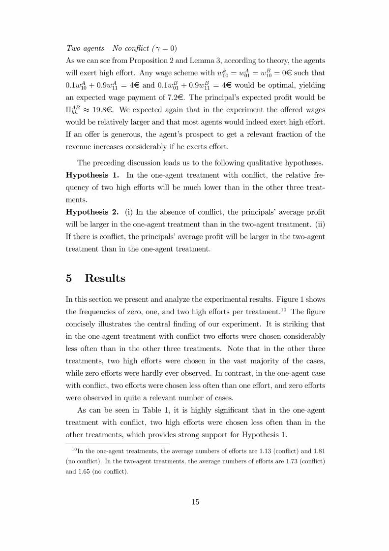
In this section we present and analyze the experimental results. Figure 1 shows

the frequencies of zero, one, and two high efforts per treatment.10 The figure

concisely illustrates the central finding of our experiment. It is striking that

in the one-agent treatment with conflict two efforts were chosen considerably

less often than in the other three treatments. Note that in the other three

treatments, two high efforts were chosen in the vast majority of the cases,

while zero efforts were hardly ever observed. In contrast, in the one-agent case

with conflict, two efforts were chosen less often than one effort, and zero efforts

were observed in quite a relevant number of cases.

As can be seen in Table 1, it is highly significant that in the one-agent

treatment with conflict, two high efforts were chosen less often than in the

other treatments, which provides strong support for Hypothesis 1.

10In the one-agent treatments, the average numbers of efforts are 1.13 (conflict) and 1.81

(no conflict). In the two-agent treatments, the average numbers of efforts are 1.73 (conflict)

and 1.65 (no conflict).

15

23.3%

40.0% 36.7%

n = 60

2.5%

22.5%

75.0%n = 40

5.3% 7.0%

87.7%n = 57

5.0%

25.0%

70.0%

n = 40

0

20

40

60

80

100

0

20

40

60

80

100

One agent − Conflict Two agents − Conflict

One agent − No conflict Two agents − No conflict

No high effort One high effort Two high efforts

Per

cent

Figure 1. Effort levels per treatment (n denotes the number of principal-

agent(s) groups per treatment). In the two-agent treatments, 86.3%

(resp., 82.5%) of the agents chose high effort if there was conflict (resp.,

no conflict).

One agent - Conflict vs.

Two agents - Conflict

One agent - Conflict vs.

One agent - No conflict

One agent - Conflict vs.

Two agents - No conflict

0.000 0.000 0.002

Two agents - Conflict vs.

One agent - No conflict

Two agents - Conflict vs.

Two agents - No conflict

One agent - No conflict vs.

Two agents - No conflict

0.174 0.803 0.039

Table 1. Significance levels for pairwise comparisons of the shares of

two high efforts between the treatments. The table reports p-values

according to two-sided Fisher exact tests.

16

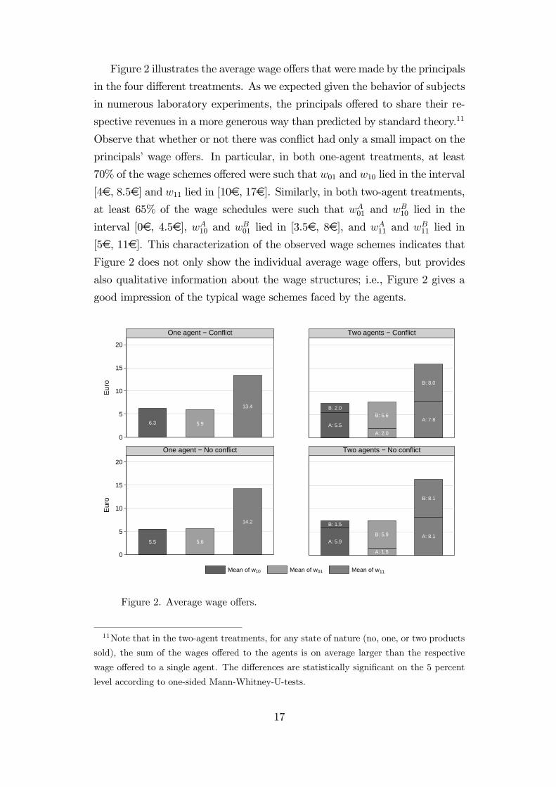
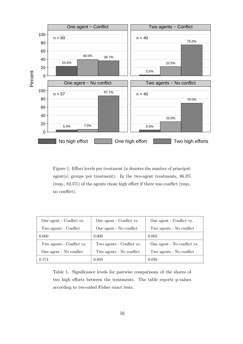
Figure 2 illustrates the average wage offers that were made by the principals

in the four different treatments. As we expected given the behavior of subjects

in numerous laboratory experiments, the principals offered to share their re-

spective revenues in a more generous way than predicted by standard theory.11

Observe that whether or not there was conflict had only a small impact on the

principals’ wage offers. In particular, in both one-agent treatments, at least

70% of the wage schemes offered were such that w01 and w10 lied in the interval

[4€, 8.5€] and w11 lied in [10€, 17€]. Similarly, in both two-agent treatments,

at least 65% of the wage schedules were such that wA01 and wB

10 lied in the

interval [0€, 4.5€], wA10 and wB

01 lied in [3.5€, 8€], and wA11 and wB

11 lied in

[5€, 11€]. This characterization of the observed wage schemes indicates that

Figure 2 does not only show the individual average wage offers, but provides

also qualitative information about the wage structures; i.e., Figure 2 gives a

good impression of the typical wage schemes faced by the agents.

6.3 5.9

13.4

5.5 5.6

14.2

0

5

10

15

20

0

5

10

15

20

Eur

oE

uro

One agent − Conflict

One agent − No conflict

Mean of w Mean of w Mean of w10 01

A: 5.5

B: 2.0

A: 2.0

B: 5.6A: 7.8

B: 8.0

A: 5.9

B: 1.5

A: 1.5

B: 5.9 A: 8.1

B: 8.1

Two agents − Conflict

Two agents − No conflict

A B

11

Figure 2. Average wage offers.

11Note that in the two-agent treatments, for any state of nature (no, one, or two products

sold), the sum of the wages offered to the agents is on average larger than the respective

wage offered to a single agent. The differences are statistically significant on the 5 percent

level according to one-sided Mann-Whitney-U-tests.

17

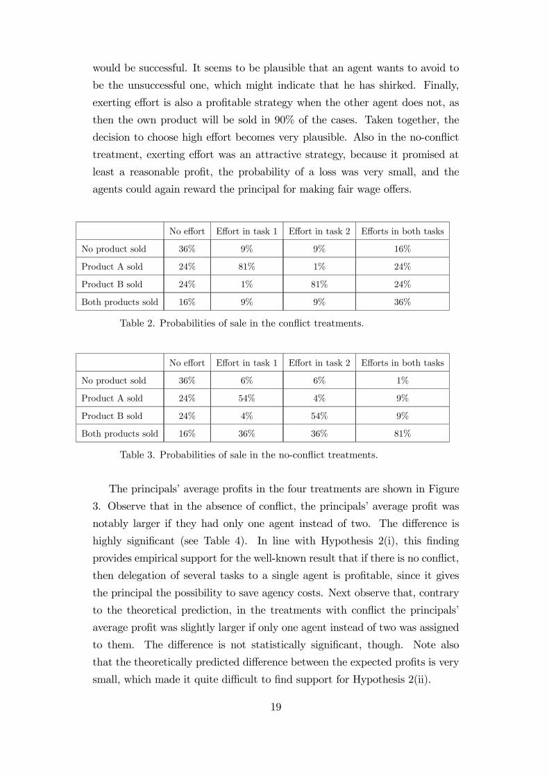
Given the typical wage schemes and Tables 2 and 3,12 the agents’ behavior

may be explained as follows. Let us first consider the one-agent treatments. In

the presence of conflict, the majority of agents may have been reluctant to ex-

ert two efforts, because then the probability of an appreciable profit (w11−4€)would be only 36%, while in 48% of the cases the profit would be very small

(w10− 4€ or w01− 4€), and a loss of 4€ would be incurred with a probabilityof 16%. On the other hand, if the agent decides to exert only one effort, the

probability of a moderate profit becomes large (82%), while the probabilities

of making either a large profit or a loss of 2€ are 9% each. Finally, exert-

ing no effort at all was a tempting strategy, since it would have resulted in

a noteworthy or even a very large profit in 64% of the cases. However, only

a minority of the agents chose to exert no effort, which may be explained by

their desire to reward the principals for their relatively generous wage offers.13

In contrast, in the absence of conflict, the vast majority of the agents chose

two high efforts, which now lead to an appreciable profit in 81% of the cases,

while the probability of making a loss was only 1%. The agents seem to have

perceived this strategy as promising and almost riskless, and hence preferred

it to the other strategies (which would have resulted in relatively small proba-

bilities of selling both products, while no product would haven been sold with

larger probabilities).14

Next, consider the two-agent treatments. In the presence of conflict, an

agent may have been very reluctant not to exert effort if he feared that the

other agent might exert effort. The reason is that if an agent exerts no effort,

the probability of sale of the own product becomes very small (10%) given

that the other agent exerts effort. Hence, with a probability of 90%, the

shirking agent’s gain would be zero or very small (wA01 or w

B10). Moreover,

if an agent exerted no effort but the other one did, then with a probability

of 81% the shirking agent would fail to sell his product, while the other one

12Notice that Tables 2 and 3 were part of the respective instructions handed out to the

participants.13Although the agents did not face fixed wages, the situation is related to the gift exchange

settings studied by Akerlof (1982) and Fehr, Kirchsteiger, and Riedl (1993).14While the presence or absence of conflict had no statistically significant impact on the

individual wage offers, in the one-agent treatments the average ratio between (w10+w01)/2

and w11 is significantly smaller in the absence (0.39) than in the presence (0.49) of conflict

(p-value = 0.002, two-sided Mann-Whitney-U-test). This finding may be seen as one further

reason why in the absence of conflict two high efforts were chosen more often.

18

would be successful. It seems to be plausible that an agent wants to avoid to

be the unsuccessful one, which might indicate that he has shirked. Finally,

exerting effort is also a profitable strategy when the other agent does not, as

then the own product will be sold in 90% of the cases. Taken together, the

decision to choose high effort becomes very plausible. Also in the no-conflict

treatment, exerting effort was an attractive strategy, because it promised at

least a reasonable profit, the probability of a loss was very small, and the

agents could again reward the principal for making fair wage offers.

No effort Effort in task 1 Effort in task 2 Efforts in both tasks

No product sold 36% 9% 9% 16%

Product A sold 24% 81% 1% 24%

Product B sold 24% 1% 81% 24%

Both products sold 16% 9% 9% 36%

Table 2. Probabilities of sale in the conflict treatments.

No effort Effort in task 1 Effort in task 2 Efforts in both tasks

No product sold 36% 6% 6% 1%

Product A sold 24% 54% 4% 9%

Product B sold 24% 4% 54% 9%

Both products sold 16% 36% 36% 81%

Table 3. Probabilities of sale in the no-conflict treatments.

The principals’ average profits in the four treatments are shown in Figure

3. Observe that in the absence of conflict, the principals’ average profit was

notably larger if they had only one agent instead of two. The difference is

highly significant (see Table 4). In line with Hypothesis 2(i), this finding

provides empirical support for the well-known result that if there is no conflict,

then delegation of several tasks to a single agent is profitable, since it gives

the principal the possibility to save agency costs. Next observe that, contrary

to the theoretical prediction, in the treatments with conflict the principals’

average profit was slightly larger if only one agent instead of two was assigned

to them. The difference is not statistically significant, though. Note also

that the theoretically predicted difference between the expected profits is very

small, which made it quite difficult to find support for Hypothesis 2(ii).

19

7.57.2

14.3

10.7

0

5

10

15

Mea

n of

pro

fits

(Eur

o)

One agent − ConflictTwo agents − Conflict

One agent − No conflictTwo agents − No conflict

Figure 3. The principals’ average profits. Recall that the theoretically

predicted expected profits are 12.16€, 13.83€, 22.02€, and 19.8€,

respectively.

One agent - Conflict vs.

Two agents - Conflict

One agent - Conflict vs.

One agent - No conflict

One agent - Conflict vs.

Two agents - No conflict

0.713 0.000 0.006

Two agents - Conflict vs.

One agent - No conflict

Two agents - Conflict vs.

Two agents - No conflict

One agent - No conflict vs.

Two agents - No conflict

0.000 0.007 0.000

Table 4. Significance levels for pairwise comparisons of the principals’

profits between the treatments. The table reports p-values according to

two-sided Mann-Whitney-U-tests.

Finally, the average wage payments that were made to the agents in the

four treatments are displayed in Table 5. As anticipated, the average payments

were larger than the expected wage payments according to standard theory.

Yet, the relative order of the magnitudes is exactly as predicted by theory. In

particular, the average wage payment in the one-agent treatment with conflict

is the smallest one, which is in line with the fact that the average number of

high efforts and thus also the average number of products a principal sold were

smallest in this treatment.

20

One agent -

Conflict

Two agents -

Conflict

One agent -

No conflict

Two agents -

No conflict

Average wage payment 7.2 8.6 11.8 12.9

Theoretical prediction 2.84 4.17 4.98 7.2

Table 5. Average wage payments in Euro.

6 Conclusion

While multi-task principal-agent models have attracted considerable attention

by contract theorists in the recent years, there is hardly any experimental evi-

dence on the problems involved. In this paper we focus on incentive problems

that arise when tasks are in direct conflict with each other. In theory, inducing

a single agent to invest effort in two conflicting tasks is difficult for the prin-

cipal, because the agent anticipates that exerting effort in one task directly

undermines the probability of success regarding the other task.

Our experimental results provide strong support for the relevance of this

incentive problem. Subjects in the experiment were indeed very reluctant to

invest simultaneously in two different tasks that are in conflict with each other.

High efforts in both tasks were observed significantly more often when the two

conflicting tasks were assigned to two different agents. In contrast, if the tasks

were unrelated, two high efforts were observed in the vast majority of cases,

regardless of whether a single agent or two different agents were in charge

of the tasks. However, in the absence of conflict, the principal’s profit was

significantly larger if both tasks were assigned to a single agent, which is in

line with the theoretical prediction.

It might be a promising avenue for future research to conduct experiments

in which the principals can choose how many agents they want to employ to

perform different tasks that may be in conflict with each other. It would then

be interesting to see whether principals would prefer to employ two agents

significantly more often when the tasks are conflicting than when they are not.

21

Appendix

Proof of Lemma 1

First observe that given that the wages cannot be negative, the agent’s par-

ticipation constraint is redundant as it is implied by (IC 3). It is imme-

diate to verify that given the symmetry of the problem, it is optimal for

the principal to set w10 = w01 = w1. Then it is straightforward to show

that w00 must be equal to zero. Thus, the reduced problem is to minimize

E [wq1q2 | a1 = a2 = 1] = (α + ρ − γ)2w11 + 2(α + ρ − γ)(1 − α − ρ + γ)w1

subject to the constraints w11 ≥ 0, w1 ≥ 0,

(α+ ρ− γ)2w11 + 2(α+ ρ− γ)(1− α− ρ+ γ)w1 − 2ψ ≥ (IC 1)

(α+ ρ)(α− γ)w11 + (α+ ρ)(1− α+ γ)w1 +

(α− γ)(1− α− ρ)w1 − ψ,

(α+ ρ− γ)2w11 + 2(α+ ρ− γ)(1− α− ρ+ γ)w1 − 2ψ ≥ (IC 3)

α2w11 + 2α(1− α)w1.

Now it is easy to see that w1 = 0 is optimal. To show this, consider a wage

scheme w11, w1 > 0. Then the LHS of the two incentive constraints are un-

changed if we change this wage scheme such that∆w1 = −∆w11α+ρ−γ

2(1−α−ρ+γ) < 0.

But now the RHS of both incentive constraints are relaxed which enables

the principal to reduce the expected compensation by reducing w1. She can

do so until w1 = 0. Then it turns out that (IC 3) is binding which implies

w11 =2ψ

(α+ρ−γ)2−α2 .

Proof of Lemma 2

In analogy to Lemma 1, it turns out that the participation constraint is redun-

dant and that w00 = 0 is optimal. In what follows, we can ignore (IC 2). Let us

verify that w01 = 0 is optimal. Consider a wage scheme with w11, w10, w01 > 0.

If we change this wage scheme such that ∆w01 = −∆w10(α+ρ)(1−α+γ)(1−α−ρ)(α−γ) < 0,

the LHS of the two remaining incentive constraints are unchanged, while both

RHS are relaxed. So the principal can increase her expected profit by lowering

w01 until w01 = 0. In the same way it is straightforward to show that it is

optimal to set w11 = 0. To see this, consider a wage scheme with w11 > 0, w10.

Then the LHS of the two incentive constraints remain unchanged if we change

this wage scheme such that ∆w11 = −∆w101−α+γα−γ < 0. Given this new wage

22

scheme, the RHS of the two incentive constraints are relaxed which implies

that the principal can increase her expected profit by lowering w11. She can

do so until w11 = 0. It is then immediate to see that the claimed solution

satisfies all the constraints.

Proof of Lemma 3

Observe that given the wages cannot be negative, each agent’s participation

constraint is redundant as it is implied by the agent’s incentive compatibility

constraint. It is straightforward to show that wA00 = wB

00 = 0. Moreover it

is immediate to verify that given the symmetry of the problem, we can solve

the problem for one agent and the other agent will receive the same incentive

scheme; i.e., wA11 = wB

11, wA10 = wB

01, and wA01 = wB

10. Let us w.l.o.g. derive the

optimal incentive scheme for agent A. The reduced problem is to minimize

(α+ ρ− γ)2wA11 + (α+ ρ− γ)(1− α− ρ+ γ)(wA

10 + wA01) subject to w

Aq1q2≥ 0

and

(α+ ρ− γ)2wA11 + (α+ ρ− γ)(1− α− ρ+ γ)(wA

10 + wA01)− ψ ≥ (IC A)

(α− γ)(α+ ρ)wA11 + (α− γ)(1− α− ρ)wA

10 + (α+ ρ)(1− α+ γ)wA01.

It is immediate to verify that in the optimal incentive scheme wA01 = 0

must hold. To see this consider a wage scheme wA11, w

A10, w

A01 > 0. The LHS

of the incentive constraint remains unchanged if we change this wage scheme

in the following way: ∆wA01 = −∆wA

10 < 0. But this relaxes the RHS of the

incentive constraint and hence enables us to lower the expected compensation

by reducing wA01 until w

A01 = 0. In the next step we can show that wA

11 = 0

is optimal. To see this consider a wage scheme wA11 > 0, wA

10. The LHS of

the incentive constraint remains unchanged if we change this wage scheme

such that ∆wA11 = −∆wA

101−α−ρ+γα+ρ−γ < 0. This relaxes the RHS of the incentive

constraint and thus makes it possible to lower the expected compensation

by reducing wA11. This can be done until w

A11 = 0. Then the result follows

immediately.

Proof of Lemma 4

In analogy to Lemma 3, the participation constraint is redundant and wA00 = 0.

To verify that wA01 = 0 is optimal, consider a wage scheme with w

A11, w

A10, w

A01 >

0. If we change this wage scheme such that ∆wA01 = −∆wA

10(α+ρ)(1−α+γ)(1−α−ρ)(α−γ) < 0,

the LHS of the incentive constraint remains unchanged, while the RHS of the

incentive constraint is relaxed. So the principal can increase her expected

23

profit by lowering wA01 until w

A01 = 0. Next, let us show that wA

11 = 0. To

see this, consider a wage scheme with wA11 > 0, w

A10. The LHS of the incentive

constraint remains unchanged if we change this wage scheme such that∆wA11 =

−∆wA101−α+γα−γ < 0. Given this new wage scheme, the RHS of the incentive

constraint is relaxed which means that the principal can increase her expected

profit by lowering wA11. She can do so until w

A11 = 0. The lemma follows

immediately.

Proof of Proposition 2

We have to show that it cannot be optimal for the principal to induce only

one effort. To show this, assume the contrary. This means the two conditions

ΠABhl > ΠAB

hh and ΠABhl > ΠAB

ll must be satisfied. The former condition can

be rewritten as R < 2ψ(α+ρ−γ)(1−α−ρ+γ)[(α+ρ−γ)(1−α−ρ+γ)−(α−γ)(1−α−ρ)](ρ−γ)−

ψ(α+ρ)(1−α+γ)[αγ+ρ(1−α+γ)](ρ−γ) and

the latter can be rewritten as R > ψ(α+ρ)(1−α+γ)[αγ+ρ(1−α+γ)](ρ−γ) . This implies that the

RHS of the former condition must be larger than the RHS of the latter, which

is equivalent to (1 − α)2 + α2 + α(ρ − γ) + (1 − α − ρ)γ < (1 − α)ρ. But

this inequality cannot hold under our assumptions. Hence, the two conditions

ΠABhl > ΠAB

hh and ΠABhl > ΠAB

ll cannot be satisfied simultaneously. Then the

proposition follows immediately.

Proof of Proposition 3

If the principal implements ai = 1 and aj 6=i = 0 in the one-agent scenario, then

she would prefer to have two agents and to implement a1 = a2 = 1. To see this,

suppose it is optimal for the principal to implement ai = 1 and aj 6=i = 0 in the

one-agent scenario. Then Πhl > Πll holds. But this means that in the two-

agent scenario ΠABhl > ΠAB

ll must be satisfied, since Πhl = ΠABhl and Πll = ΠAB

ll .

But we know from Proposition 2 that if ΠABhl > ΠAB

ll , then ΠABhh > ΠAB

hl = Πhl.

It remains to be shown that there exists a unique γ̂ ∈ (0,min {α, ρ}) suchthatΠhh(γ̂) = ΠAB

hh (γ̂).Observe thatΠhh−ΠABhh > 0 if γ = 0 andΠhh−ΠAB

hh < 0

if γ = min {α, ρ} . Moreover, the condition Πhh − ΠABhh > 0 is equivalent to

f(·) := γ(3αρ + ρ2 + α2 − ρ − 2α) + γ2(1 − α − ρ) + ρα − ρα2 − ρ2α > 0.

The derivative of f(·) with respect to γ is given by df(·)dγ

= (2γ − α − ρ)(1 −α − ρ) − (1 − ρ)α < 0. Hence, a simple intermediate value argument implies

that there exists a unique γ̂ ∈ (0,min {α, ρ}) such that Πhh(γ̂) = ΠABhh (γ̂).

The remainder of the proposition follows immediately from Proposition 1 and

Proposition 2.

24

References

Akerlof, G., 1982, “Labor Contracts as Partial Gift Exchange,” Quarterly Journal

of Economics, 97, 543—569.

Baron, D.P. and D. Besanko, 1992, “Information, Control, and Organizational

Structure,” Journal of Economics and Management Strategy, 1, 237—275.

Bolton, P. and M. Dewatripont, 2005, Contract Theory, Cambridge, MA: MIT

Press.

Brüggen, A. and F. Moers, 2007, “The Role of Financial Incentives and Social

Incentives in Multi-Task Settings,” Journal of Management Accounting Re-

search, 19, 25—50.

Camerer, C.F., 2003, Behavioral Game Theory: Experiments in Strategic Interac-

tion, Princeton: Princeton University Press.

Che, Y.-K. and S.-W. Yoo, 2001, “Optimal Incentives for Teams,” American Eco-

nomic Review, 91, 525—541.

Dana, J.D., Jr., 1993, “The Organization and Scope of Agents: Regulating Multi-

product Industries,” Journal of Economic Theory, 59, 288—310.

Dewatripont, M., I. Jewitt and J. Tirole, 2000, “Multitask Agency Problems: Focus

and Task Clustering,” European Economic Review, 44, 869—877.

Dewatripont, M. and J. Tirole, 1999, “Advocates,” Journal of Political Economy,

107, 1—39.

Fehr, E., G. Kirchsteiger and A. Riedl, 1993, “Does Fairness Prevent Market Clear-

ing? An Experimental Investigation,” Quarterly Journal of Economics, 108,

437-459.

Fehr, E. and K.M. Schmidt, 2004, “Fairness and Incentives in a Multi-task Principal-

Agent Model,” Scandinavian Journal of Economics, 106, 453—474.

Fehr, E. and K.M. Schmidt, 2006, The Economics of Fairness, Reciprocity and

Altruism - Experimental Evidence and New Theories, in: Handbook on the

Economics of Giving, Reciprocity and Altruism, Vol. 1, ed. by S.-C. Kolm and

J.M. Ythier, Amsterdam: Elsevier, 615—691.

Fischbacher, U., 2007, z-Tree: Zurich Toolbox for Ready-made Economic Experi-

ments, Experimental Economics, 10, 171—178.

25

Gilbert, R.J. and M.H. Riordan, 1995, “Regulating Complementary Products: A

Comparative Institutional Analysis,” RAND Journal of Economics, 26, 243—

256.

Greiner, B., 2004, An Online Recruiting System for Economic Experiments, in:

Forschung und wissenschaftliches Rechnen 2003. GWDG Bericht 63, ed. by

K. Kremer and V. Macho, Göttingen: Ges. für Wiss. Datenverarbeitung, 79—

93.

Hirao, Y., 1993, “Task Assignment and Agency Structures,” Journal of Economics

and Management Strategy, 2, 299—323.

Holmström, B. and P. Milgrom, 1991, “Multitask Principal-Agent Analyses: In-

centive Contracts, Asset Ownership, and Job Design.” Journal of Law, Eco-

nomics, and Organization, 7, 24—52.

Innes, R.D., 1990, “Limited Liability and Incentive Contracting with Ex-ante Ac-

tion Choices,” Journal of Economic Theory, 52, 45—67.

Khalil, F., D. Kim and D. Shin, 2006, “Optimal Task Design: To Integrate or Sepa-

rate Planning and Implementation?,” Journal of Economics and Management

Strategy, 15, 457—478.

Kim, S.K., 1997, “Limited Liability and Bonus Contracts,” Journal of Economics

and Management Strategy, 6, 899—913.

Laffont, J.-J. and D. Martimort, 2002, The Theory of Incentives: The Principal-

Agent Model. Princeton, N.J.: Princeton University Press.

Laux, C., 2001, “Limited-Liability and Incentive Contracting with Multiple Projects,”

RAND Journal of Economics, 32, 514—526.

Mylovanov, T. and P.W. Schmitz, 2008, “Task Scheduling and Moral Hazard,”

Economic Theory, 37, 307—320.

Park, E.-S., 1995, “Incentive Contracting under Limited Liability,” Journal of Eco-

nomics and Management Strategy, 4, 477—490.

Pitchford, R., 1998, “Moral hazard and limited liability: The real effects of contract

bargaining,” Economics Letters, 61, 251—259.

Schmitz, P.W., 2005, “Allocating Control in Agency Problems with Limited Li-

ability and Sequential Hidden Actions”, RAND Journal of Economics, 36,

318—336.

Tirole, J., 2001, “Corporate Governance,” Econometrica, 69, 1—35.

26

Supplementary material

The following instructions and comprehension questions were handed out to the participants in the treatment with one agent and conflict ( γ = 0.3): Experimental instructions In this experiment, you can earn money. Your payoff depends on your decisions and on other participants’ decisions. During the whole experiment communication is not allowed. If you have a question, please raise your hand out of the cabin. All decisions are anonymous; i.e., no participant ever learns the identity of a person who has made a particular decision. The payment is conducted anonymously, too; i.e., no participant learns what the payoff of another participant is. In this experiment, you will either be a merchant or a sales representative with equal probability. Each merchant is matched with exactly one sales representative. As soon as the experiment starts, you will learn whether you have been assigned to the role of a merchant or to the role of a sales representative. The merchant can sell exactly one unit of a product A and exactly one unit of a product B via his sales representative. Product A and product B are similar. The merchant receives a revenue of 15 Euro for each product sold. He can pay his sales representative a wage depending on the number of products sold. (Suppose that the costs the merchant had to incur when purchasing the products are not relevant in this experiment. Furthermore, the merchant does not have to bear any stockkeeping costs if product A or product B is not sold.) The sales representative can promote each product A and B individually. If the sales representative does not promote any product, the probability of sale of each product is 40%. If the sales representative promotes a product, the probability of sale of this product increases by 50 percentage points while the probability of sale of the other product decreases by 30 percentage points. The sales representative can either promote no product, or promote exactly one product, or promote both products. Depending on the number of products promoted, the probabilities of sale read as follows:

- If the sales representative does not promote any product, then each product will be sold with a probability of 40%.

- If the sales representative promotes only product A, then product A will be sold with a probability of 40% + 50% = 90%, and product B will be sold with a probability of 40% - 30% = 10%.

- If the sales representative promotes only product B, then product B will be sold with a probability of 40% + 50% = 90%, and product A will be sold with a probability of 40% - 30% = 10%.

- If the sales representative promotes both products, then product A and product B will be sold with a probability of 40% + 50% - 30% = 60% each.

As the products are similar, promotion for one product does not only have a positive effect on the probability of sale of the promoted product, but it has also a negative effect on the probability of sale of the other product.

i

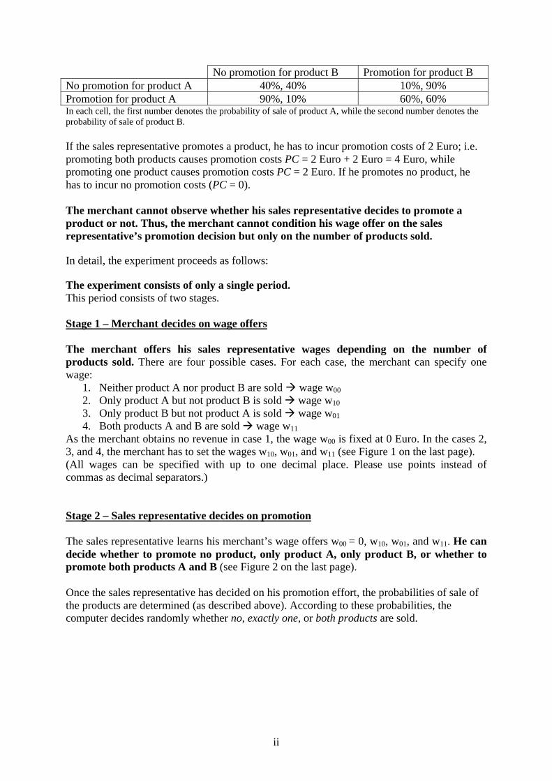
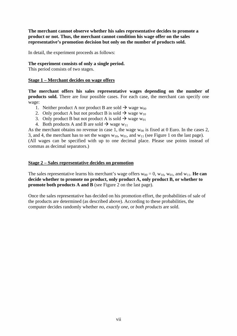
No promotion for product B Promotion for product B No promotion for product A 40%, 40% 10%, 90% Promotion for product A 90%, 10% 60%, 60% In each cell, the first number denotes the probability of sale of product A, while the second number denotes the probability of sale of product B. If the sales representative promotes a product, he has to incur promotion costs of 2 Euro; i.e. promoting both products causes promotion costs PC = 2 Euro + 2 Euro = 4 Euro, while promoting one product causes promotion costs PC = 2 Euro. If he promotes no product, he has to incur no promotion costs (PC = 0). The merchant cannot observe whether his sales representative decides to promote a product or not. Thus, the merchant cannot condition his wage offer on the sales representative’s promotion decision but only on the number of products sold. In detail, the experiment proceeds as follows: The experiment consists of only a single period. This period consists of two stages. Stage 1 – Merchant decides on wage offers The merchant offers his sales representative wages depending on the number of products sold. There are four possible cases. For each case, the merchant can specify one wage:

1. Neither product A nor product B are sold wage w00 2. Only product A but not product B is sold wage w10 3. Only product B but not product A is sold wage w01 4. Both products A and B are sold wage w11

As the merchant obtains no revenue in case 1, the wage w00 is fixed at 0 Euro. In the cases 2, 3, and 4, the merchant has to set the wages w10, w01, and w11 (see Figure 1 on the last page). (All wages can be specified with up to one decimal place. Please use points instead of commas as decimal separators.) Stage 2 – Sales representative decides on promotion The sales representative learns his merchant’s wage offers w00 = 0, w10, w01, and w11. He can decide whether to promote no product, only product A, only product B, or whether to promote both products A and B (see Figure 2 on the last page). Once the sales representative has decided on his promotion effort, the probabilities of sale of the products are determined (as described above). According to these probabilities, the computer decides randomly whether no, exactly one, or both products are sold.

ii

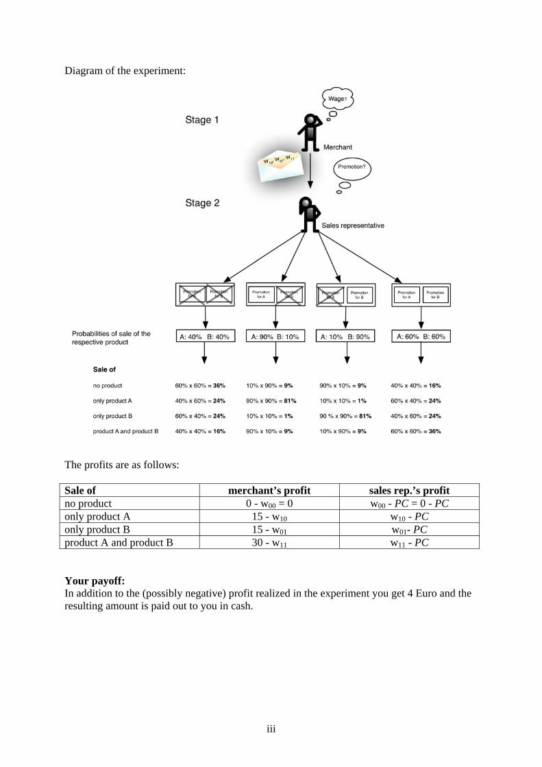
Diagram of the experiment:

The profits are as follows: Sale of merchant’s profit sales rep.’s profit no product 0 - w00 = 0 w00 - PC = 0 - PC only product A 15 - w10 w10 - PC only product B 15 - w01 w01- PC product A and product B 30 - w11 w11 - PC Your payoff: In addition to the (possibly negative) profit realized in the experiment you get 4 Euro and the resulting amount is paid out to you in cash.

iii

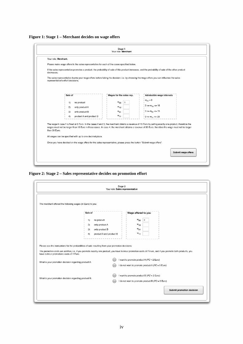
Figure 1: Stage 1 – Merchant decides on wage offers

Figure 2: Stage 2 – Sales representative decides on promotion effort

iv

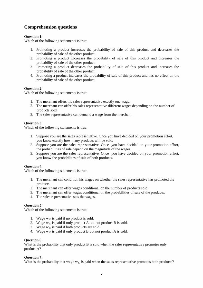
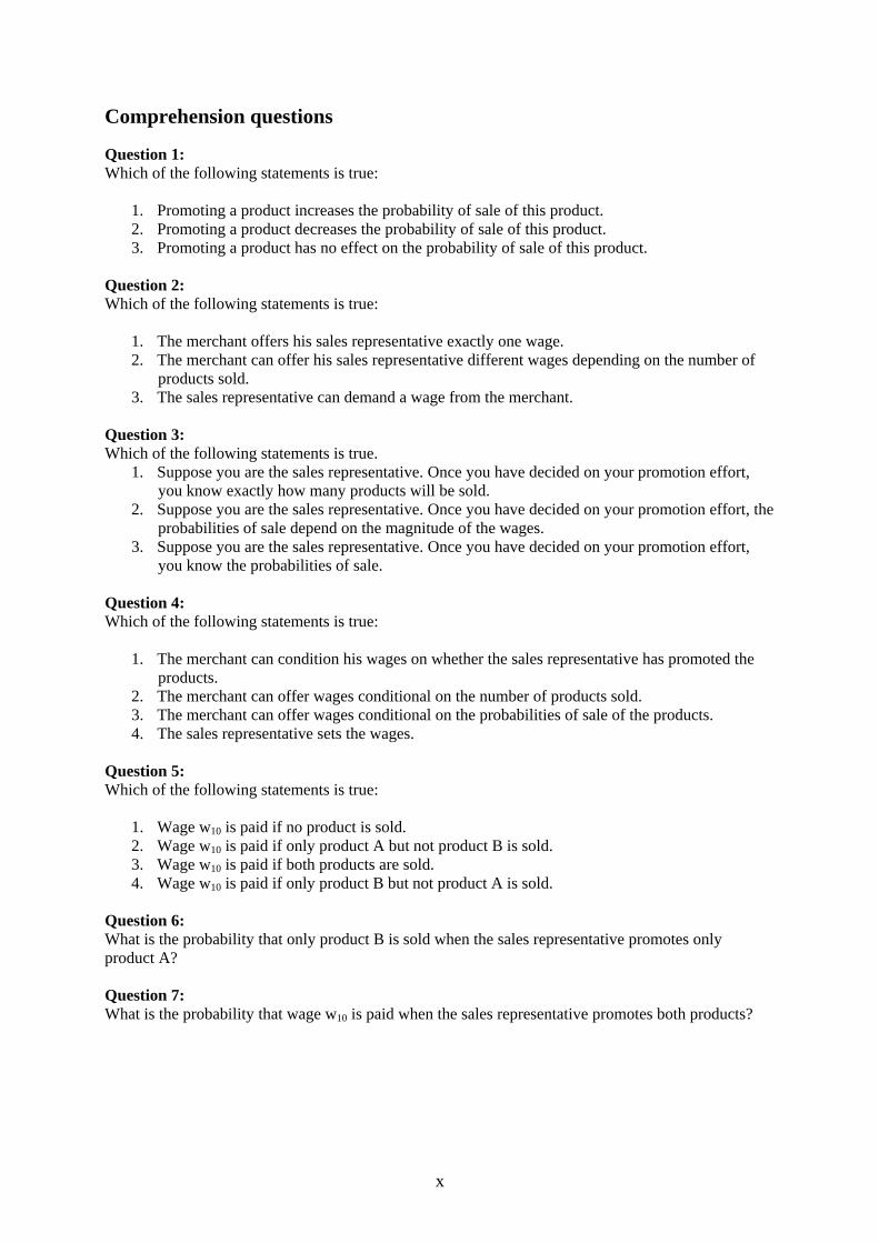
Comprehension questions Question 1: Which of the following statements is true:

1. Promoting a product increases the probability of sale of this product and decreases the probability of sale of the other product.

2. Promoting a product increases the probability of sale of this product and increases the probability of sale of the other product.

3. Promoting a product decreases the probability of sale of this product and increases the probability of sale of the other product.

4. Promoting a product increases the probability of sale of this product and has no effect on the probability of sale of the other product.

Question 2: Which of the following statements is true:

1. The merchant offers his sales representative exactly one wage. 2. The merchant can offer his sales representative different wages depending on the number of

products sold. 3. The sales representative can demand a wage from the merchant.

Question 3: Which of the following statements is true:

1. Suppose you are the sales representative. Once you have decided on your promotion effort, you know exactly how many products will be sold.

2. Suppose you are the sales representative. Once you have decided on your promotion effort, the probabilities of sale depend on the magnitude of the wages.

3. Suppose you are the sales representative. Once you have decided on your promotion effort, you know the probabilites of sale of both products.

Question 4: Which of the following statements is true:

1. The merchant can condition his wages on whether the sales representative has promoted the products.

2. The merchant can offer wages conditional on the number of products sold. 3. The merchant can offer wages conditional on the probabilities of sale of the products. 4. The sales representative sets the wages.

Question 5: Which of the following statements is true:

1. Wage w10 is paid if no product is sold. 2. Wage w10 is paid if only product A but not product B is sold. 3. Wage w10 is paid if both products are sold. 4. Wage w10 is paid if only product B but not product A is sold.

Question 6: What is the probability that only product B is sold when the sales representative promotes only product A? Question 7: What is the probability that wage w10 is paid when the sales representative promotes both products?

v

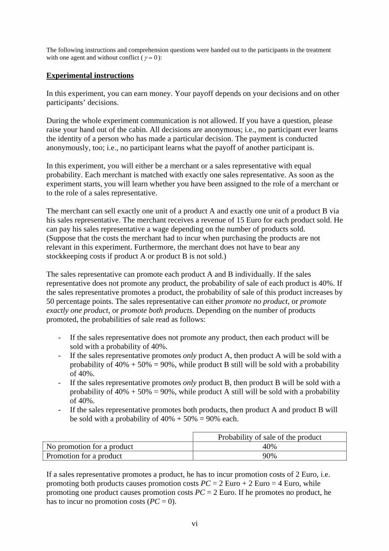
The following instructions and comprehension questions were handed out to the participants in the treatment with one agent and without conflict ( γ = 0): Experimental instructions In this experiment, you can earn money. Your payoff depends on your decisions and on other participants’ decisions. During the whole experiment communication is not allowed. If you have a question, please raise your hand out of the cabin. All decisions are anonymous; i.e., no participant ever learns the identity of a person who has made a particular decision. The payment is conducted anonymously, too; i.e., no participant learns what the payoff of another participant is. In this experiment, you will either be a merchant or a sales representative with equal probability. Each merchant is matched with exactly one sales representative. As soon as the experiment starts, you will learn whether you have been assigned to the role of a merchant or to the role of a sales representative. The merchant can sell exactly one unit of a product A and exactly one unit of a product B via his sales representative. The merchant receives a revenue of 15 Euro for each product sold. He can pay his sales representative a wage depending on the number of products sold. (Suppose that the costs the merchant had to incur when purchasing the products are not relevant in this experiment. Furthermore, the merchant does not have to bear any stockkeeping costs if product A or product B is not sold.) The sales representative can promote each product A and B individually. If the sales representative does not promote any product, the probability of sale of each product is 40%. If the sales representative promotes a product, the probability of sale of this product increases by 50 percentage points. The sales representative can either promote no product, or promote exactly one product, or promote both products. Depending on the number of products promoted, the probabilities of sale read as follows:

- If the sales representative does not promote any product, then each product will be sold with a probability of 40%.

- If the sales representative promotes only product A, then product A will be sold with a probability of 40% + 50% = 90%, while product B still will be sold with a probability of 40%.

- If the sales representative promotes only product B, then product B will be sold with a probability of 40% + 50% = 90%, while product A still will be sold with a probability of 40%.

- If the sales representative promotes both products, then product A and product B will be sold with a probability of 40% + 50% = 90% each.

Probability of sale of the product No promotion for a product 40% Promotion for a product 90% If a sales representative promotes a product, he has to incur promotion costs of 2 Euro, i.e. promoting both products causes promotion costs PC = 2 Euro + 2 Euro = 4 Euro, while promoting one product causes promotion costs PC = 2 Euro. If he promotes no product, he has to incur no promotion costs (PC = 0).

vi

The merchant cannot observe whether his sales representative decides to promote a product or not. Thus, the merchant cannot condition his wage offer on the sales representative’s promotion decision but only on the number of products sold. In detail, the experiment proceeds as follows: The experiment consists of only a single period. This period consists of two stages. Stage 1 – Merchant decides on wage offers The merchant offers his sales representative wages depending on the number of products sold. There are four possible cases. For each case, the merchant can specify one wage:

1. Neither product A nor product B are sold wage w00 2. Only product A but not product B is sold wage w10 3. Only product B but not product A is sold wage w01 4. Both products A and B are sold wage w11

As the merchant obtains no revenue in case 1, the wage w00 is fixed at 0 Euro. In the cases 2, 3, and 4, the merchant has to set the wages w10, w01, and w11 (see Figure 1 on the last page). (All wages can be specified with up to one decimal place. Please use points instead of commas as decimal separators.) Stage 2 – Sales representative decides on promotion The sales representative learns his merchant’s wage offers w00 = 0, w10, w01, and w11. He can decide whether to promote no product, only product A, only product B, or whether to promote both products A and B (see Figure 2 on the last page). Once the sales representative has decided on his promotion effort, the probabilities of sale of the products are determined (as described above). According to these probabilities, the computer decides randomly whether no, exactly one, or both products are sold.

vii

Diagram of the experiment:

The profits are specified as follows: Sale of merchant's profit sales rep.'s profit no product 0 - w00 = 0 w00 - PC = 0 - PC only product A 15 - w10 w10 - PC only product B 15 - w01 w01- PC product A and product B 30 - w11 w11 - PC Your payoff: In addition to the (possibly negative) profit realized in the experiment you get 4 Euro and the resulting amount is paid out to you in cash.

viii

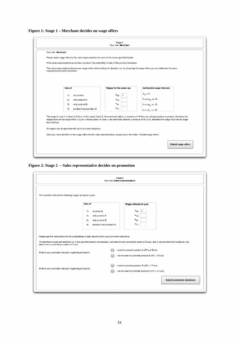
Figure 1: Stage 1 – Merchant decides on wage offers

Figure 2: Stage 2 – Sales representative decides on promotion

ix

Comprehension questions Question 1: Which of the following statements is true:

1. Promoting a product increases the probability of sale of this product. 2. Promoting a product decreases the probability of sale of this product. 3. Promoting a product has no effect on the probability of sale of this product.

Question 2: Which of the following statements is true:

1. The merchant offers his sales representative exactly one wage. 2. The merchant can offer his sales representative different wages depending on the number of

products sold. 3. The sales representative can demand a wage from the merchant.

Question 3: Which of the following statements is true.

1. Suppose you are the sales representative. Once you have decided on your promotion effort, you know exactly how many products will be sold.

2. Suppose you are the sales representative. Once you have decided on your promotion effort, the probabilities of sale depend on the magnitude of the wages.

3. Suppose you are the sales representative. Once you have decided on your promotion effort, you know the probabilities of sale.

Question 4: Which of the following statements is true:

1. The merchant can condition his wages on whether the sales representative has promoted the products.

2. The merchant can offer wages conditional on the number of products sold. 3. The merchant can offer wages conditional on the probabilities of sale of the products. 4. The sales representative sets the wages.

Question 5: Which of the following statements is true:

1. Wage w10 is paid if no product is sold. 2. Wage w10 is paid if only product A but not product B is sold. 3. Wage w10 is paid if both products are sold. 4. Wage w10 is paid if only product B but not product A is sold.

Question 6: What is the probability that only product B is sold when the sales representative promotes only product A? Question 7: What is the probability that wage w10 is paid when the sales representative promotes both products?

x

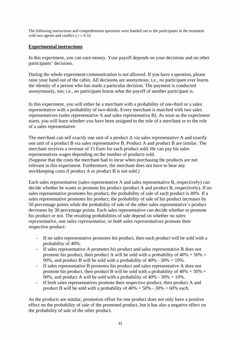
The following instructions and comprehension questions were handed out to the participants in the treatment with two agents and conflict ( γ = 0.3): Experimental instructions In this experiment, you can earn money. Your payoff depends on your decisions and on other participants’ decisions. During the whole experiment communication is not allowed. If you have a question, please raise your hand out of the cabin. All decisions are anonymous; i.e., no participant ever learns the identity of a person who has made a particular decision. The payment is conducted anonymously, too; i.e., no participant learns what the payoff of another participant is.

In this experiment, you will either be a merchant with a probability of one-third or a sales representative with a probability of two-thirds. Every merchant is matched with two sales representatives (sales representative A and sales representative B). As soon as the experiment starts, you will learn whether you have been assigned to the role of a merchant or to the role of a sales representative. The merchant can sell exactly one unit of a product A via sales representative A and exactly one unit of a product B via sales representative B. Product A and product B are similar. The merchant receives a revenue of 15 Euro for each product sold. He can pay his sales representatives wages depending on the number of products sold. (Suppose that the costs the merchant had to incur when purchasing the products are not relevant in this experiment. Furthermore, the merchant does not have to bear any stockkeeping costs if product A or product B is not sold.) Each sales representative (sales representative A and sales representative B, respectively) can decide whether he wants to promote his product (product A and product B, respectively). If no sales representative promotes his product, the probability of sale of each product is 40%. If a sales representative promotes his product, the probability of sale of his product increases by 50 percentage points while the probability of sale of the other sales representative’s product decreases by 30 percentage points. Each sales representative can decide whether to promote his product or not. The resulting probabilities of sale depend on whether no sales representative, one sales representative, or both sales representatives promote their respective product:

- If no sales representative promotes his product, then each product will be sold with a probability of 40%.

- If sales representative A promotes his product and sales representative B does not promote his product, then product A will be sold with a probability of 40% + 50% = 90%, and product B will be sold with a probability of 40% - 30% = 10%.

- If sales representative B promotes his product and sales representative A does not promote his product, then product B will be sold with a probability of 40% + 50% = 90%, and product A will be sold with a probability of 40% - 30% = 10%.

- If both sales representatives promote their respective product, then product A and product B will be sold with a probability of 40% + 50% - 30% = 60% each.

As the products are similar, promotion effort for one product does not only have a positive effect on the probability of sale of the promoted product, but it has also a negative effect on the probability of sale of the other product.

xi

Sales representative B does not promote product

B promotes product

B does not promote product A

40%, 40% 10%, 90% Sales representative A promotes product A 90%, 10% 60%, 60% In each cell, the first number denotes the probability of sale of product A, while the

second number denotes the probability of sale of product B. If a sales representative promotes his product, he has to incur promotion costs PC = 2 Euro. If a sales representative does not promote his product, he does not have to incur promotion costs (PC = 0 Euro). The merchant cannot observe whether his sales representatives decide to promote their products or not. Thus, the merchant cannot condition his wage offers on the sales representatives’ promotion decisions but only on the number of products sold. A sales representative also cannot observe the promotion decision of the other sales representative. In detail, the experiment proceeds as follows: The experiment consists of only a single period. This period consists of two stages. Stage 1 – Merchant decides on wage offers The merchant offers his sales representatives wages depending on the number of products sold. There are four possible cases. For each case, the merchant can specify one wage:

1. neither product A nor product B are sold wage for sales representative A and for sales representative B Aw00

Bw00

2. only product A but not product B is sold wage for sales representative A and for sales representative B Aw10

Bw10

3. only product B but not product A is sold wage for sales representative A and for sales representative B Aw01

Bw01

4. both products A and B are sold wage for sales representative A and for sales representative B Aw11

Bw11

As the merchant obtains no revenue in case 1, the wages and are fixed at 0 Euro. In the cases 2, 3, and 4, the merchant has to set the wages and , and , and

for his sales representatives A and B (see Figure 1 on the last page).

Aw00Aw10

Bw00Bw10

Aw01Bw01

Aw11Bw11

(All wages can be specified with up to one decimal place. Please use points instead of commas as decimal separators.) Stage 2 – Sales representatives A and B decide on promotion The sales representatives A and B learn every wage offer the merchant has made in stage 1. Thus, a sales representative knows the wages he may receive as well as the wages that the merchant may pay to the other sales representative.

xii

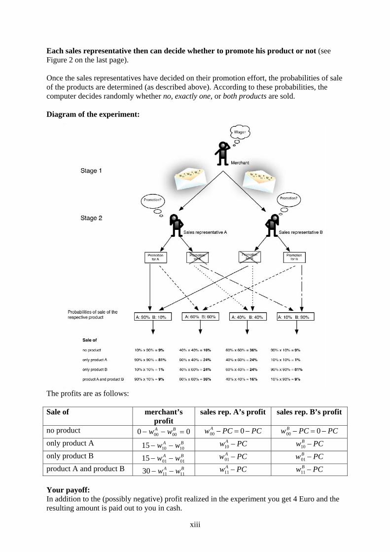
Each sales representative then can decide whether to promote his product or not (see Figure 2 on the last page). Once the sales representatives have decided on their promotion effort, the probabilities of sale of the products are determined (as described above). According to these probabilities, the computer decides randomly whether no, exactly one, or both products are sold. Diagram of the experiment:

The profits are as follows: Sale of merchant’s

profit sales rep. A’s profit sales rep. B’s profit

no product 00 0000 =−− BA ww w00A − PC = 0− PC w00

B − PC = 0− PC only product A BA ww 101015 −− w10

A − PC w10B − PC

only product B BA ww 010115 −− w01A − PC w01

B − PC product A and product B BA ww 111130 −− w11

A − PC w11B − PC

Your payoff: In addition to the (possibly negative) profit realized in the experiment you get 4 Euro and the resulting amount is paid out to you in cash.

xiii

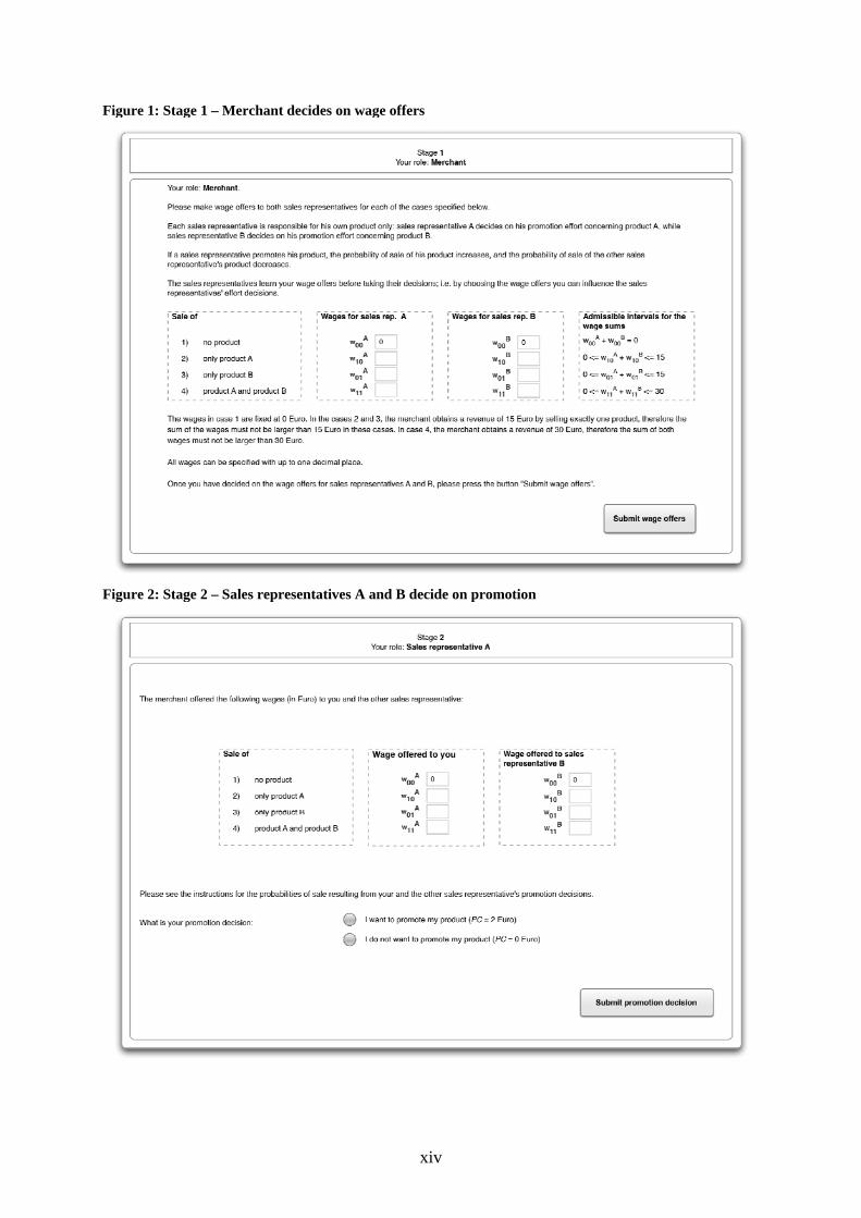
Figure 1: Stage 1 – Merchant decides on wage offers

Figure 2: Stage 2 – Sales representatives A and B decide on promotion

xiv

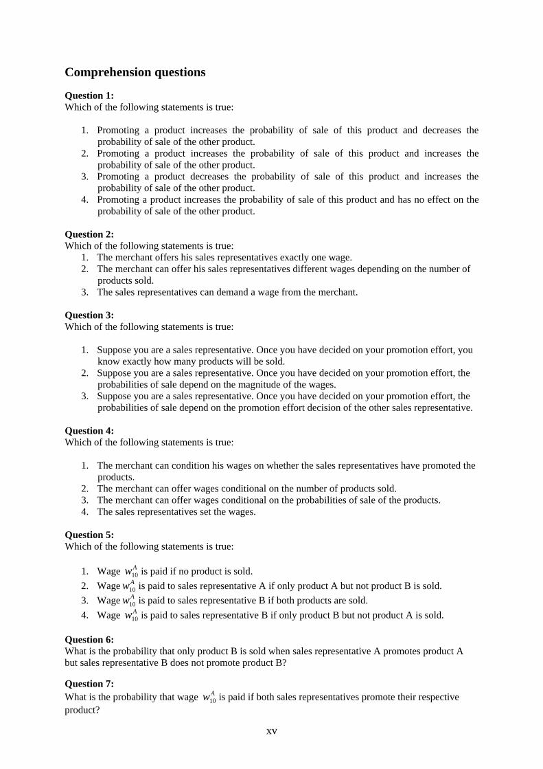
Comprehension questions Question 1: Which of the following statements is true:

1. Promoting a product increases the probability of sale of this product and decreases the probability of sale of the other product.

2. Promoting a product increases the probability of sale of this product and increases the probability of sale of the other product.

3. Promoting a product decreases the probability of sale of this product and increases the probability of sale of the other product.

4. Promoting a product increases the probability of sale of this product and has no effect on the probability of sale of the other product.

Question 2: Which of the following statements is true:

1. The merchant offers his sales representatives exactly one wage. 2. The merchant can offer his sales representatives different wages depending on the number of

products sold. 3. The sales representatives can demand a wage from the merchant.

Question 3: Which of the following statements is true:

1. Suppose you are a sales representative. Once you have decided on your promotion effort, you know exactly how many products will be sold.

2. Suppose you are a sales representative. Once you have decided on your promotion effort, the probabilities of sale depend on the magnitude of the wages.

3. Suppose you are a sales representative. Once you have decided on your promotion effort, the probabilities of sale depend on the promotion effort decision of the other sales representative.

Question 4: Which of the following statements is true:

1. The merchant can condition his wages on whether the sales representatives have promoted the products.

2. The merchant can offer wages conditional on the number of products sold. 3. The merchant can offer wages conditional on the probabilities of sale of the products. 4. The sales representatives set the wages.

Question 5: Which of the following statements is true:

1. Wage w10A is paid if no product is sold.

2. Wage w10A is paid to sales representative A if only product A but not product B is sold.

3. Wage w10A is paid to sales representative B if both products are sold.

4. Wage w10A is paid to sales representative B if only product B but not product A is sold.

Question 6: What is the probability that only product B is sold when sales representative A promotes product A but sales representative B does not promote product B? Question 7: What is the probability that wage is paid if both sales representatives promote their respective product?

w10A

xv

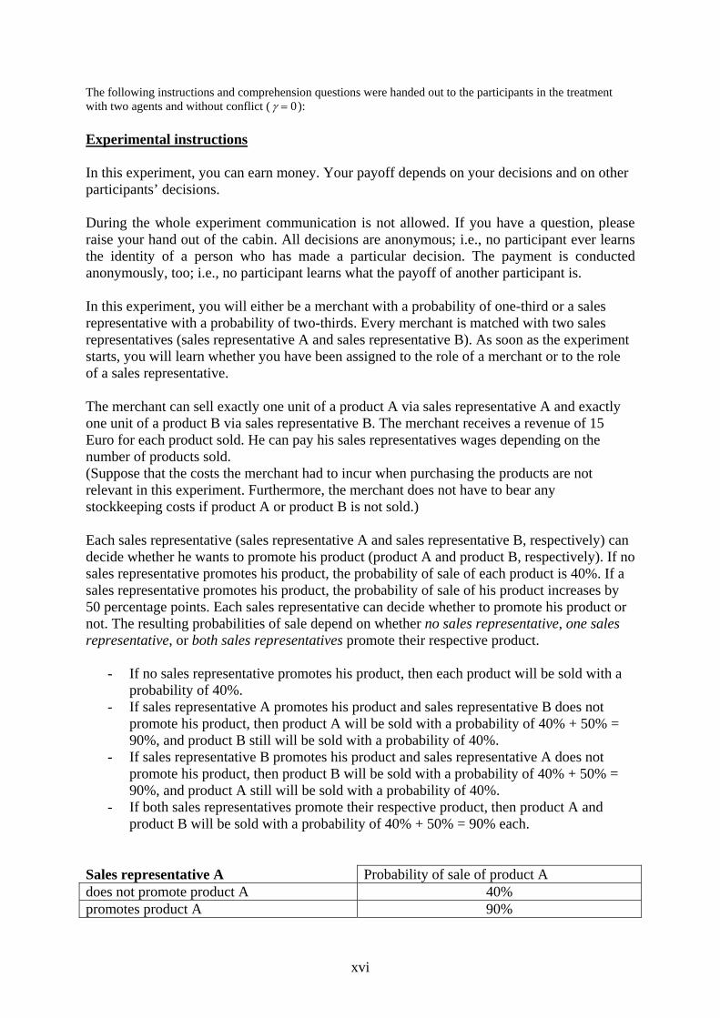
The following instructions and comprehension questions were handed out to the participants in the treatment with two agents and without conflict ( γ = 0): Experimental instructions In this experiment, you can earn money. Your payoff depends on your decisions and on other participants’ decisions. During the whole experiment communication is not allowed. If you have a question, please raise your hand out of the cabin. All decisions are anonymous; i.e., no participant ever learns the identity of a person who has made a particular decision. The payment is conducted anonymously, too; i.e., no participant learns what the payoff of another participant is. In this experiment, you will either be a merchant with a probability of one-third or a sales representative with a probability of two-thirds. Every merchant is matched with two sales representatives (sales representative A and sales representative B). As soon as the experiment starts, you will learn whether you have been assigned to the role of a merchant or to the role of a sales representative. The merchant can sell exactly one unit of a product A via sales representative A and exactly one unit of a product B via sales representative B. The merchant receives a revenue of 15 Euro for each product sold. He can pay his sales representatives wages depending on the number of products sold. (Suppose that the costs the merchant had to incur when purchasing the products are not relevant in this experiment. Furthermore, the merchant does not have to bear any stockkeeping costs if product A or product B is not sold.) Each sales representative (sales representative A and sales representative B, respectively) can decide whether he wants to promote his product (product A and product B, respectively). If no sales representative promotes his product, the probability of sale of each product is 40%. If a sales representative promotes his product, the probability of sale of his product increases by 50 percentage points. Each sales representative can decide whether to promote his product or not. The resulting probabilities of sale depend on whether no sales representative, one sales representative, or both sales representatives promote their respective product.

- If no sales representative promotes his product, then each product will be sold with a probability of 40%.

- If sales representative A promotes his product and sales representative B does not promote his product, then product A will be sold with a probability of 40% + 50% = 90%, and product B still will be sold with a probability of 40%.

- If sales representative B promotes his product and sales representative A does not promote his product, then product B will be sold with a probability of 40% + 50% = 90%, and product A still will be sold with a probability of 40%.

- If both sales representatives promote their respective product, then product A and product B will be sold with a probability of 40% + 50% = 90% each.

Sales representative A Probability of sale of product A does not promote product A 40% promotes product A 90%

xvi

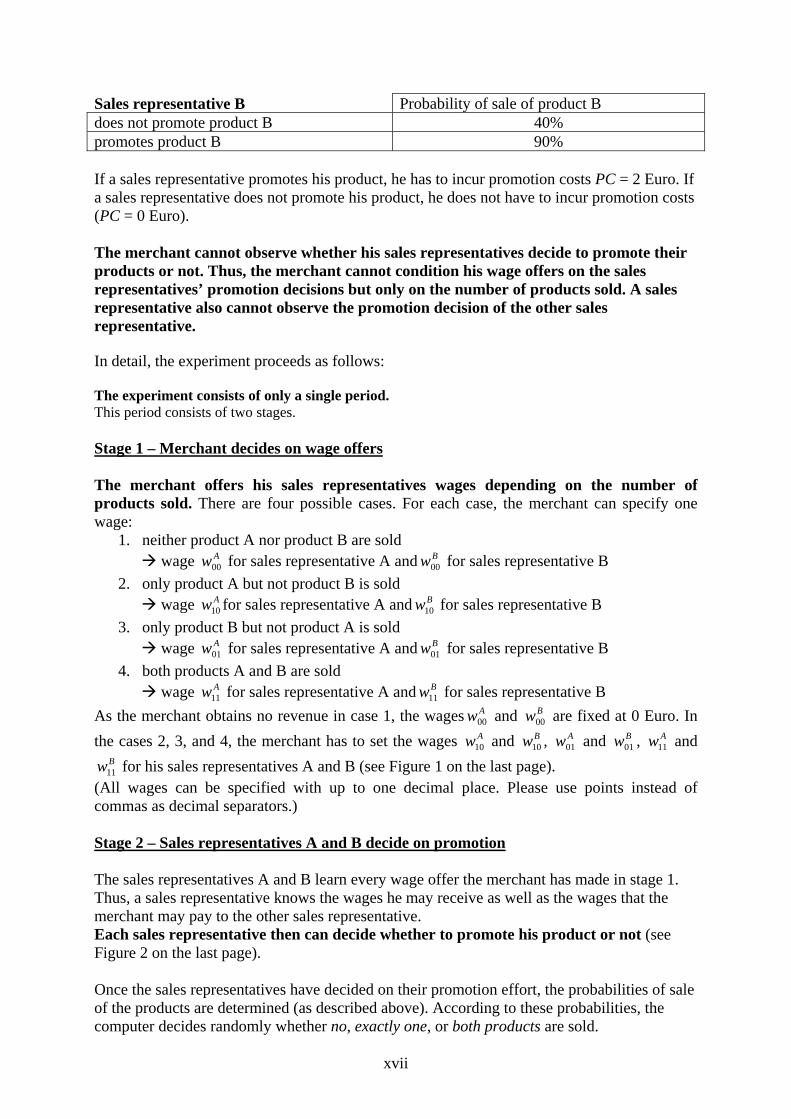
Sales representative B Probability of sale of product B does not promote product B 40% promotes product B 90% If a sales representative promotes his product, he has to incur promotion costs PC = 2 Euro. If a sales representative does not promote his product, he does not have to incur promotion costs (PC = 0 Euro). The merchant cannot observe whether his sales representatives decide to promote their products or not. Thus, the merchant cannot condition his wage offers on the sales representatives’ promotion decisions but only on the number of products sold. A sales representative also cannot observe the promotion decision of the other sales representative. In detail, the experiment proceeds as follows: The experiment consists of only a single period. This period consists of two stages. Stage 1 – Merchant decides on wage offers The merchant offers his sales representatives wages depending on the number of products sold. There are four possible cases. For each case, the merchant can specify one wage:

1. neither product A nor product B are sold wage for sales representative A and for sales representative B Aw00

Bw00

2. only product A but not product B is sold wage for sales representative A and for sales representative B Aw10

Bw10

3. only product B but not product A is sold wage for sales representative A and for sales representative B Aw01

Bw01

4. both products A and B are sold wage for sales representative A and for sales representative B Aw11

Bw11

As the merchant obtains no revenue in case 1, the wages and are fixed at 0 Euro. In the cases 2, 3, and 4, the merchant has to set the wages and , and , and

for his sales representatives A and B (see Figure 1 on the last page).

Aw00Aw10

Bw00Bw10

Aw01Bw01

Aw11Bw11

(All wages can be specified with up to one decimal place. Please use points instead of commas as decimal separators.) Stage 2 – Sales representatives A and B decide on promotion The sales representatives A and B learn every wage offer the merchant has made in stage 1. Thus, a sales representative knows the wages he may receive as well as the wages that the merchant may pay to the other sales representative. Each sales representative then can decide whether to promote his product or not (see Figure 2 on the last page). Once the sales representatives have decided on their promotion effort, the probabilities of sale of the products are determined (as described above). According to these probabilities, the computer decides randomly whether no, exactly one, or both products are sold.

xvii

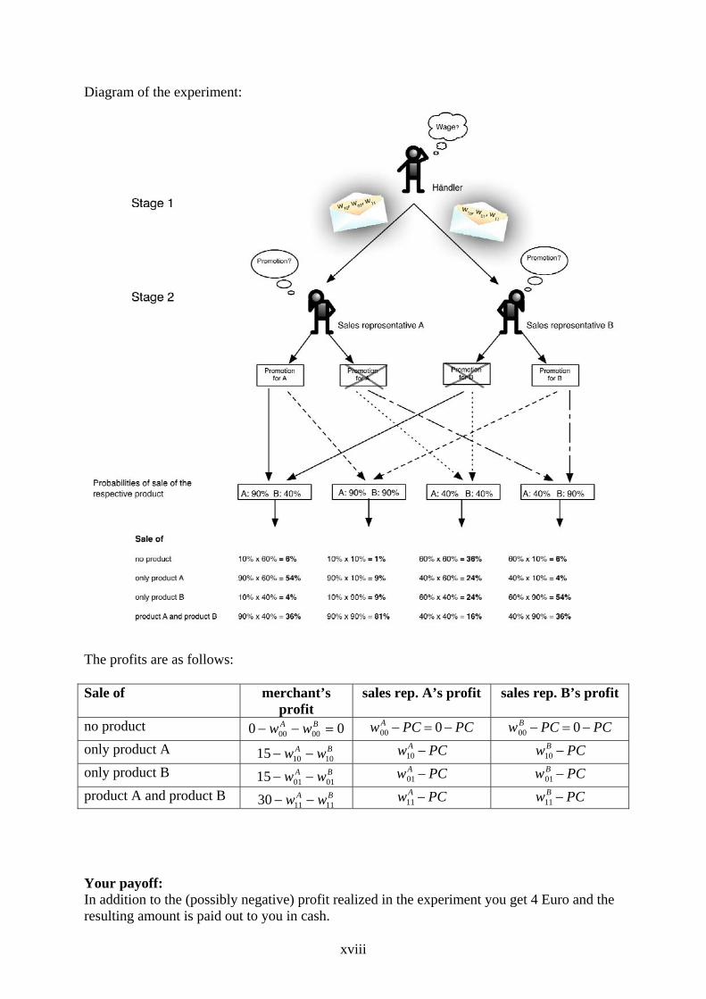
Diagram of the experiment:

The profits are as follows: Sale of merchant’s

profit sales rep. A’s profit sales rep. B’s profit

no product 00 0000 =−− BA ww w00A − PC = 0− PC w00

B − PC = 0− PC only product A BA ww 101015 −− w10

A − PC w10B − PC

only product B BA ww 010115 −− w01A − PC w01

B − PC product A and product B BA ww 111130 −− w11

A − PC w11B − PC

Your payoff: In addition to the (possibly negative) profit realized in the experiment you get 4 Euro and the resulting amount is paid out to you in cash.

xviii

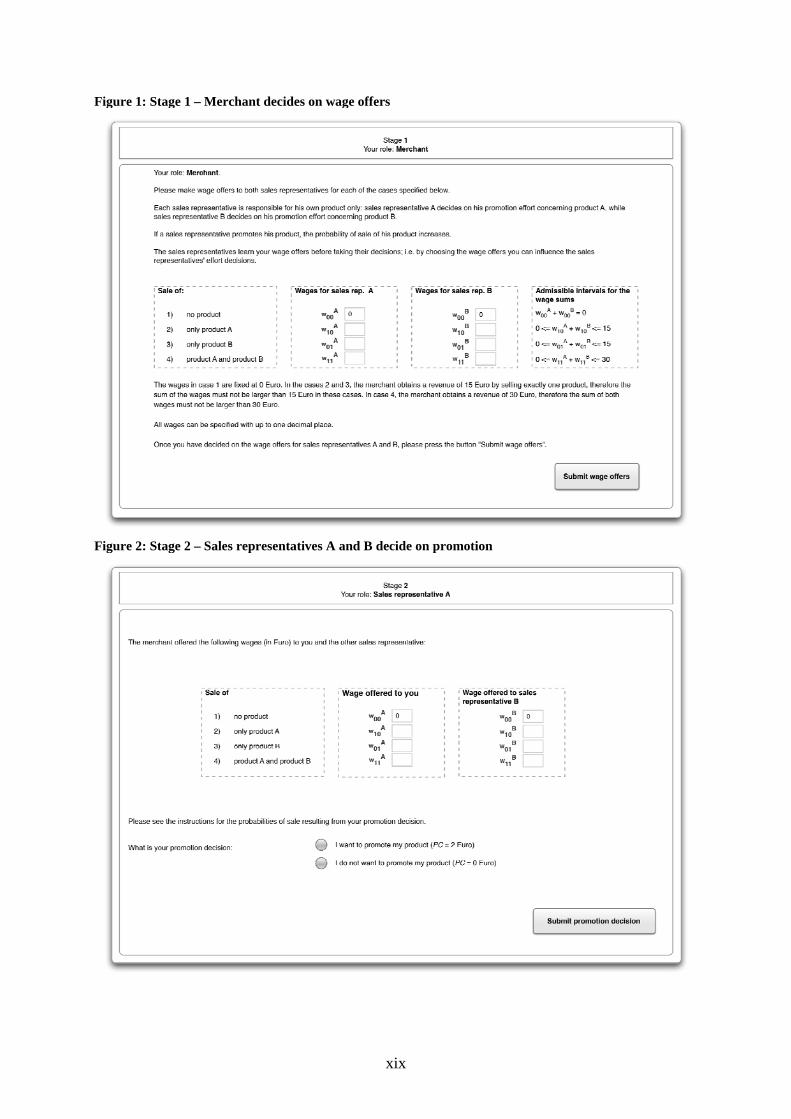
Figure 1: Stage 1 – Merchant decides on wage offers

Figure 2: Stage 2 – Sales representatives A and B decide on promotion

xix

Comprehension questions Question 1: Which of the following statements is true:

1. Promoting a product increases the probability of sale of this product. 2. Promoting a product decreases the probability of sale of this product. 3. Promoting a product has no effect on the probability of sale of this product.

Question 2: Which of the following statements is true:

1. The merchant offers his sales representatives exactly one wage. 2. The merchant can offer his sales representatives different wages depending on the number of

products sold. 3. The sales representatives can demand a wage from the merchant.

Question 3: Which of the following statements is true:

1. Suppose you are a sales representative. Once you have decided on your promotion effort, your product will be sold with certainty.

2. Suppose you are a sales representative. Once you have decided on your promotion effort, the probabilities of sale depend on the magnitude of the wages.

3. Suppose you are a sales representative. Once you have decided on your promotion effort, you know the probability of sale of your product.

Question 4: Which of the following statements is true:

1. The merchant can condition his wages on whether the sales representatives have promoted the products.

2. The merchant can offer wages conditional on the number of products sold. 3. The merchant can offer wages conditional on the probabilities of sale of the products. 4. The sales representatives set the wages.

Question 5: Which of the following statements is true:

1. Wage w10A is paid if no product is sold.

2. Wage w10A is paid to sales representative A if only product A but not product B is sold.

3. Wage w10A is paid to sales representative B if both products are sold.

4. Wage w10A is paid to sales representative B if only product B but not product A is sold.

Question 6: What is the probability that only product B is sold when sales representative A promotes product A but sales representative B does not promote product B? Question 7: What is the probability that wage is paid if both sales representatives promote their respective product?

w10A

xx