1

Paper 2588-2018

Confirmatory Factor Analysis in SAS®:

Application to Public Administration

Niloofar Ramezani, George Mason University; Kevin Gittner, University of Northern Colorado

ABSTRACT

When hypothesizing the factor structure of latent variables in a study, confirmatory factor analysis (CFA) is the appropriate method to confirm factor structure of responses. Learning about building CFA within any statistical package is beneficial as it enables researchers to find evidence for validity of instruments. An instrument was developed by Wright (2016) to assess Community-Based Development Organizations’ (CBDO) ability to build capacity. This study addresses the continued development of the instrument’s structure using CFA in SAS® 9.4 and examines how it contributes to enhancing an organization’s ability to create sustainable communities. Developing and evaluating the instrument is crucial due to the growing role of CBDOs in the offering of public services, yet the significant gap that exists in the literature about organizational factors affecting CBDO’s ability to build capacity. The purpose of the data analysis is to investigate this scale's factor structure of responses and address the capacity of nonprofits within the United States by surveying 1,000 organizations. Different steps for performing CFA in SAS, using primarily the CALIS procedure, are explored and their strengths and limitations are specified. Results are compared to the similar model built in Mplus, which is recommended for latent variable models. Suggestions for best practices are provided through the methodological comparison of results.

INTRODUCTION

Factor analysis is a statistical technique used to find a set of unobserved, also known as latent, variables or factors that can account for the covariance among a larger set of observed, also known as manifest, variables. A factor is an unobservable variable that is assumed to influence observed variables. Factor analysis is also used to assess the validity, and reliability, of measurement scales (Carmines & Zeller, 1979).

Through factor analysis, the underlying dimensions of the observed variables and the variables corresponding to each of the underlying dimensions can be identified. These underlying dimensions are the continuous latent variables or factors and the observed variables are the factor indicators. There are two types of factor analysis: CFA and exploratory factor analysis (EFA).

EFA is an exploratory technique to determine the dimensionality of a set of variables and observe the pattern of the factor loadings. However, CFA relies on the existing knowledge about the dimensionality of a set of variables for a given population based on theory or previous research. Applying CFA as a confirmatory tool enables the researchers to investigate whether the established dimensionality and factor-loading pattern fits a new sample from the same, or a new, population. CFA applies restrictions on factor loadings as well as their variance, covariance, and correlation. Unlike EFA, CFA can include correlated residuals when minor factors influence the variables. Although CFA is most directly relevant for evaluating the internal structure of a scale, it also provides information related to the internal consistency of the scale. Additionally, CFA can be used to evaluate convergent and discriminant evidence. The importance and advantages of CFA makes it crucial to investigate different tools for performing it in various software packages, including SAS and Mplus within this paper, and compare their performance.

CONFIRMATORY FACTOR ANALYSIS

Latent variables, also known as unmeasured variables or latent factors, are hypothesized constructs that cannot be directly observed. The existence of a latent variable can only be inferred by the way that it influences manifest variables, that can be directly observed, or other latent variables.

As explained in the introduction section, rather than using the exploratory approach of an EFA to simply determine the number and meaning of different factors, if there exists sufficient evidence, and knowledge,

2

about the structure of the data, researchers and practitioners can use a confirmatory approach to evaluate the internal structure of a newly designed scale (Kline, 1999).

The dimensionality or internal structure of a scale has inferences for reliability and validity. The internal structure of a scale reflects its internal consistency by showing which items are consistent with what other items; this is relevant to the reliability of a scale that needs to be addressed when developing a new instrument. The internal structure of a scale also helps with the appropriate interpretation of scale scores to show the match between the internal structures of the scale with its intended construct(s); this is related to validity, which is another important aspect to be addressed for a new instrument development.

Two software packages are used within this study to perform a CFA. They are Mplus version 7.31 (Los Angeles, CA) and SAS PROC CALIS. Assessment of the CFA is based on both global fit indices and item diagnostic statistics including standardized factor loadings, modification indices, and the squared multiple correlation. The global fit indices were used to determine appropriate model fit. Tests and fit indices that were used included the 𝜒2 test, which was based on the weighted least squares mean variance estimation (WLSMV; Muthén, 1998–2004), the comparative fit index (CFI; Bentler, 1990), Tucker Lewis fit index (TLI; Tucker & Lewis, 1973), root mean square error approximation (RMSEA; Browne & Cudeck, 1992; Steiger, 2007), and the weighted root mean squared residual (WRMR; Muthén, 1998–2004). The suggested cutoff level for an appropriate fitting model is to have a CFI ≥ .95 or TLI ≥ .95, and RMSEA < 0.06 with a goal of having .05 within the 90% confidence interval (Browne & Cudeck, 1992; Hu & Bentler, 1999; Steiger, 2007). For the current study, smaller values of WRMR were sought with a goal of getting close to 1.0 (Yu, 2002). Within SAS, slightly different methods needed to be used due to its limitations in performing the WLSMV estimation method.

For item diagnostics, the cutoff values are more ambiguous. Decisions are up to the researchers, as they should be looking for the best fitting items (DiStefano, Zhu, & Mindrila, 2009). If the modification indices are too large, the standardized factor loadings are too small, or the squared multiple correlation is too small, we would consider making modifications to our model based on these justifications (Schreiber, Nora, Stage, Barlow, & King, 2006). All of the above information was used to assess how well the original baseline hypothesized model fits the data.

SOFTWARE COMPARISON

This section focuses on exploring the capabilities of the different software packages for conducting a CFA using the observed and latent variables. Documentation for all the software packages reviewed can be found in the following sources: for the SAS procedure, SAS PROC CALIS, we recommend SAS STAT User’s Guide: The CALIS Procedure; for Mplus procedure, we recommend Mplus User’s Guide (Muthen and Muthen 1998–2010). Both of the aforementioned documentations were comprehensive and user-friendly (Narayanan, 2012).

Mplus has the capability of estimating CFA models, and CFA models with background variables, for a single or multiple groups while the factor indicators can be continuous, censored, categorical, ordinal, counts, or any combinations of these variable types. When factor indicators are all continuous, Mplus has seven estimator choices: maximum likelihood (ML), maximum likelihood with robust standard errors and chi-square (MLR, MLF, MLM, MLMV), generalized least squares (GLS), and weighted least squares (WLS) also referred to as ADF. When at least one factor indicator is binary, categorical, or ordinal, Mplus has seven estimator choices: weighted least squares (WLS), robust weighted least squares (WLSM, WLSMV), maximum likelihood (ML), maximum likelihood with robust standard errors and chi-square (MLR, MLF), and unweighted least squares (ULS). These options are limited within SAS especially when dealing with skewed indicators. When at least one factor indicator is censored, unordered categorical, or a count, Mplus has six estimator choices: weighted least squares (WLS), robust weighted least squares (WLSM, WLSMV), maximum likelihood (ML), and maximum likelihood with robust standard errors and chi-square (MLR, MLF).

Therefore, Mplus integrates modeling framework to handle continuous, categorical, observed, and latent variables and when data sets include missing observations, it incorporates some missing data handling techniques to handle them. SAS PROC CALIS integrates other analysis capabilities available in SAS (e.g., PROC MI and PROC MIANALYZE for missing data) which is beneficial when having missing data.

3

DATASET

This section is dedicated to explaining the instrument and data used for this study.

PUBLIC ADMINISTRATION BACKGROUND

Nonprofit organizations play an important role in the provision of public goods to society. Nonprofits are voluntary, and self-governing, organizations that serve the public interests as well as the objectives of its constituents (Boris, 2010).Government has called upon nonprofits to take a leading role in delivering health and human services to people in need. This interdependence has challenged nonprofits and government to form effective collaborations to find better ways in responding to the needs of society (Salamon 2002).

Nonprofit activity has been growing is in the delivery of community-based services. For many decades, government has worked with community-based nonprofits to improve living situation in low-income neighborhoods. This relationship has been vital in the revitalization of economic activity in inner city neighborhoods (Rubin, 2001; Schill, 1996; Vidal, 1999). This continued reliance on community based development organizations (CBDO) by the federal, state, and local government has challenged CBDOs to think tactically about how to develop comprehensive community-building efforts in creating sustainable communities.

Scholars highlight the significance of strategy identification, by the CBDOs, in building organizational capacity if addressing issues related to economic development, jobs, and the environment is part of the goal of such organizations. However, there is a gap in the literature, particularly related to empirical evidence identifying, regarding the nature of the factors of organizational capacity that influence a CBDO’s effectiveness in the revitalization of neighborhoods. In theory, local governments contract-out with CBDOs for the provision of services. However, little is known about what elements of CBDO organizational capacity affect a CBDOs ability to administer these projects (Fredericksen & London, 2003). This gap in the literature was addressed by investigating the impact of capacity building strategies and the ability of CBDOs to build sustainable communities by Wright (2016).

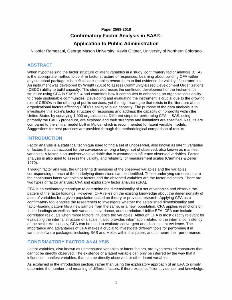
The survey used for collecting the data used for this study utilizes existing theories and studies regarding different tactics used by community based nonprofits to build organizational capacity as well as the previously developed model of CBDO capacity components. The CBDO capacity model recognizes five components that comprise CBDO capacity which are shown in figure 1. These five components of CBDO capacity have unique elements and varying impacts on organizational performance: resource capacity measures the ability for the CBDO to attract grants, donors, loans, and contracts. Organizational capacity is focused on the internal management structure of the organization. Programmatic capacity focuses on a CBDO’s ability to build and manage its community and economic development activities in their service areas. Networking capacity is the ability of a CBDO to form strategic partnerships with other community based nonprofits, private enterprises, and local government. Finally, political capacity measures the ability of a CBDO to effectively advocate on behalf of community residents and mobilize support locally around issues important to the organization and community as a whole.

To identify the specific ways in which community based development organizations build capacity and explain the relationship between nonprofit organizational effectiveness and components of CBDO capacity, a new instrument was developed by Wright (2016) which CFA could assist with checking its validity and reliability.

4

Figure 1. Five components of CBDO capacity

INSUTRUMENT AND DATA

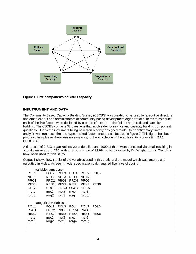
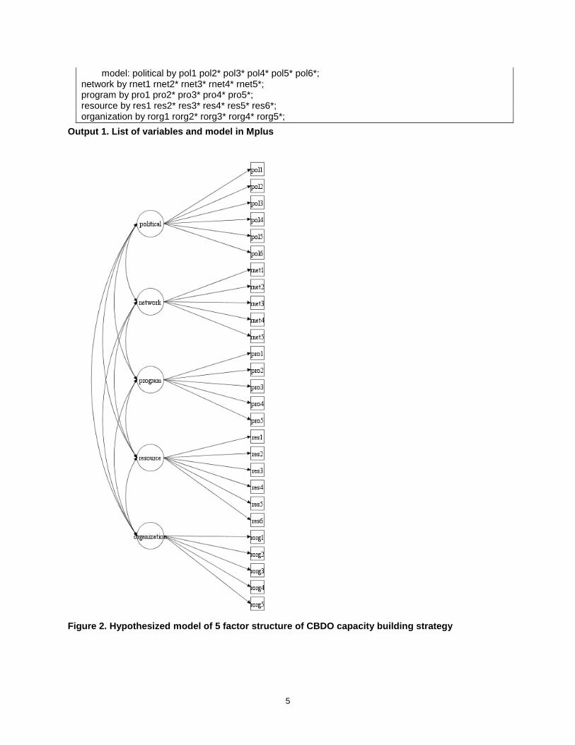
The Community Based Capacity Building Survey (CBCBS) was created to be used by executive directors and other leaders and administrators of community-based development organizations. Items to measure each of the five factors were designed by a group of experts in the field of non-profit and capacity building. The CBCBS contains 32 questions that involve demographics and capacity building component questions. Due to the instrument being based on a newly designed model, this confirmatory factor analysis was run to confirm the hypothesized factor structure as detailed in figure 2. This figure has been produced in Mplus as there was no easy way, to the knowledge of the authors, to produce it in SAS PROC CALIS.

A database of 2,713 organizations were identified and 1000 of them were contacted via email resulting in a total sample size of 352, with a response rate of 12.9%, to be collected by Dr. Wright’s team. This data have been used for this study.

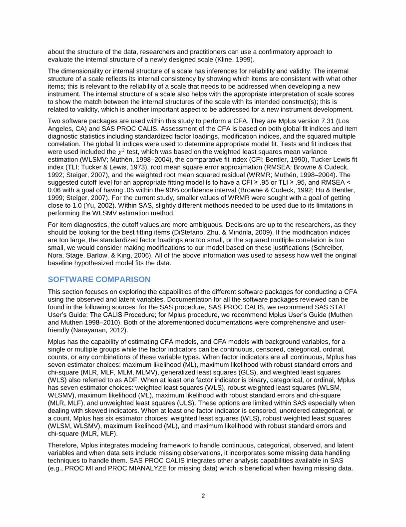
Output 1 shows how the list of the variables used in this study and the model which was entered and outputted in Mplus. As seen, model specification only required five lines of coding.

variable names are POL1 POL2 POL3 POL4 POL5 POL6 NET1 NET2 NET3 NET4 NET5 PRO1 PRO2 PRO3 PRO4 PRO5 RES1 RES2 RES3 RES4 RES5 RES6 ORG1 ORG2 ORG3 ORG4 ORG5 rnet1 rnet2 rnet3 rnet4 rnet5 rorg1 rorg2 rorg3 rorg4 rorg5; categorical variables are POL1 POL2 POL3 POL4 POL5 POL6 PRO1 PRO2 PRO3 PRO4 PRO5 RES1 RES2 RES3 RES4 RES5 RES6 rnet1 rnet2 rnet3 rnet4 rnet5 rorg1 rorg2 rorg3 rorg4 rorg5;

5

model: political by pol1 pol2* pol3* pol4* pol5* pol6*; network by rnet1 rnet2* rnet3* rnet4* rnet5*; program by pro1 pro2* pro3* pro4* pro5*; resource by res1 res2* res3* res4* res5* res6*; organization by rorg1 rorg2* rorg3* rorg4* rorg5*;

Output 1. List of variables and model in Mplus

Figure 2. Hypothesized model of 5 factor structure of CBDO capacity building strategy

6

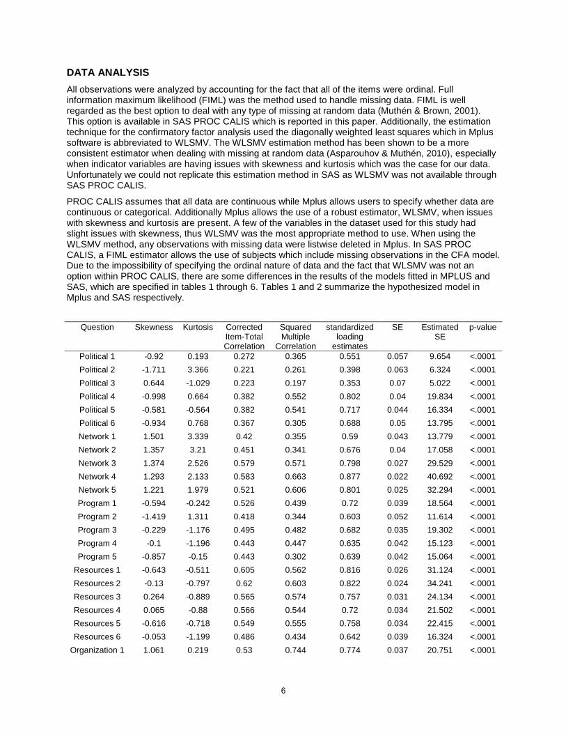
DATA ANALYSIS

All observations were analyzed by accounting for the fact that all of the items were ordinal. Full information maximum likelihood (FIML) was the method used to handle missing data. FIML is well regarded as the best option to deal with any type of missing at random data (Muthén & Brown, 2001). This option is available in SAS PROC CALIS which is reported in this paper. Additionally, the estimation technique for the confirmatory factor analysis used the diagonally weighted least squares which in Mplus software is abbreviated to WLSMV. The WLSMV estimation method has been shown to be a more consistent estimator when dealing with missing at random data (Asparouhov & Muthén, 2010), especially when indicator variables are having issues with skewness and kurtosis which was the case for our data. Unfortunately we could not replicate this estimation method in SAS as WLSMV was not available through SAS PROC CALIS.

PROC CALIS assumes that all data are continuous while Mplus allows users to specify whether data are continuous or categorical. Additionally Mplus allows the use of a robust estimator, WLSMV, when issues with skewness and kurtosis are present. A few of the variables in the dataset used for this study had slight issues with skewness, thus WLSMV was the most appropriate method to use. When using the WLSMV method, any observations with missing data were listwise deleted in Mplus. In SAS PROC CALIS, a FIML estimator allows the use of subjects which include missing observations in the CFA model. Due to the impossibility of specifying the ordinal nature of data and the fact that WLSMV was not an option within PROC CALIS, there are some differences in the results of the models fitted in MPLUS and SAS, which are specified in tables 1 through 6. Tables 1 and 2 summarize the hypothesized model in Mplus and SAS respectively.

Question Skewness Kurtosis Corrected Item-Total Correlation

Squared Multiple

Correlation

standardized loading

estimates

SE Estimated SE

p-value

Political 1 -0.92 0.193 0.272 0.365 0.551 0.057 9.654 <.0001

Political 2 -1.711 3.366 0.221 0.261 0.398 0.063 6.324 <.0001

Political 3 0.644 -1.029 0.223 0.197 0.353 0.07 5.022 <.0001

Political 4 -0.998 0.664 0.382 0.552 0.802 0.04 19.834 <.0001

Political 5 -0.581 -0.564 0.382 0.541 0.717 0.044 16.334 <.0001

Political 6 -0.934 0.768 0.367 0.305 0.688 0.05 13.795 <.0001

Network 1 1.501 3.339 0.42 0.355 0.59 0.043 13.779 <.0001

Network 2 1.357 3.21 0.451 0.341 0.676 0.04 17.058 <.0001

Network 3 1.374 2.526 0.579 0.571 0.798 0.027 29.529 <.0001

Network 4 1.293 2.133 0.583 0.663 0.877 0.022 40.692 <.0001

Network 5 1.221 1.979 0.521 0.606 0.801 0.025 32.294 <.0001

Program 1 -0.594 -0.242 0.526 0.439 0.72 0.039 18.564 <.0001

Program 2 -1.419 1.311 0.418 0.344 0.603 0.052 11.614 <.0001

Program 3 -0.229 -1.176 0.495 0.482 0.682 0.035 19.302 <.0001

Program 4 -0.1 -1.196 0.443 0.447 0.635 0.042 15.123 <.0001

Program 5 -0.857 -0.15 0.443 0.302 0.639 0.042 15.064 <.0001

Resources 1 -0.643 -0.511 0.605 0.562 0.816 0.026 31.124 <.0001

Resources 2 -0.13 -0.797 0.62 0.603 0.822 0.024 34.241 <.0001

Resources 3 0.264 -0.889 0.565 0.574 0.757 0.031 24.134 <.0001

Resources 4 0.065 -0.88 0.566 0.544 0.72 0.034 21.502 <.0001

Resources 5 -0.616 -0.718 0.549 0.555 0.758 0.034 22.415 <.0001

Resources 6 -0.053 -1.199 0.486 0.434 0.642 0.039 16.324 <.0001

Organization 1 1.061 0.219 0.53 0.744 0.774 0.037 20.751 <.0001

7

Organization 2 0.867 0.157 0.44 0.686 0.602 0.041 14.537 <.0001

Organization 3 1.041 0.06 0.51 0.752 0.776 0.035 22.402 <.0001

Organization 4 0.942 0.028 0.488 0.582 0.678 0.04 16.788 <.0001

Organization 5 0.892 -0.062 0.467 0.694 0.672 0.041 16.517 <.0001

Table 1. Hypothesized model in Mplus using WLSMV

Question Error Variance

Total Variance

R-Square standardized Estimate

SE t-value P-value

Political 1 0.7222 0.92406 0.2184 0.46738 0.05027 9.2975 <.0001

Political 2 0.54397 0.61913 0.1214 0.34844 0.05491 6.3451 <.0001

Political 3 1.76797 2.05763 0.1408 0.3752 0.05325 7.046 <.0001

Political 4 0.3417 0.86441 0.6047 0.77763 0.03417 22.7585 <.0001

Political 5 0.72759 1.47673 0.5073 0.71225 0.03658 19.4709 <.0001

Political 6 0.43153 0.57728 0.2525 0.50248 0.04821 10.4226 <.0001

Network 1 0.62469 0.97088 0.3566 0.59713 0.03061 19.5101 <.0001

Network 2 0.56606 0.89063 0.3644 0.60367 0.03289 18.353 <.0001

Network 3 0.54266 1.23503 0.5606 0.74874 0.02519 29.7207 <.0001

Network 4 0.41558 1.14151 0.6359 0.79746 0.02671 29.8556 <.0001

Network 5 0.5956 1.31297 0.5464 0.73917 0.02805 26.3541 <.0001

Program 1 0.53194 0.84364 0.3695 0.60784 0.04397 13.8244 <.0001

Program 2 0.9161 1.23487 0.2581 0.50808 0.04873 10.4255 <.0001

Program 3 1.02553 1.83099 0.4399 0.66325 0.04421 15.0037 <.0001

Program 4 1.08546 1.84248 0.4109 0.64099 0.04556 14.0696 <.0001

Program 5 0.9792 1.36068 0.2804 0.52949 0.04726 11.2048 <.0001

Resources 1 0.58891 1.34615 0.5625 0.75001 0.02966 25.2843 <.0001

Resources 2 0.4575 1.25011 0.634 0.79626 0.02611 30.4966 <.0001

Resources 3 0.72857 1.51848 0.5202 0.72125 0.03195 22.5768 <.0001

Resources 4 0.78276 1.44257 0.4574 0.6763 0.03544 19.0837 <.0001

Resources 5 0.73167 1.50672 0.5144 0.71721 0.03209 22.3477 <.0001

Resources 6 1.20321 1.76079 0.3167 0.56273 0.04306 13.0677 <.0001

Organization 1 0.52232 0.86851 0.3986 0.63134 0.03487 18.1074 <.0001

Organization 2 0.84627 1.17083 0.2772 0.52651 0.03467 15.185 <.0001

Organization 3 0.51321 1.20558 0.5743 0.75783 0.02735 27.7127 <.0001

Organization 4 0.92484 1.65078 0.4398 0.66314 0.02695 24.6055 <.0001

Organization 5 0.87593 1.5933 0.4502 0.671 0.0284 23.6301 <.0001

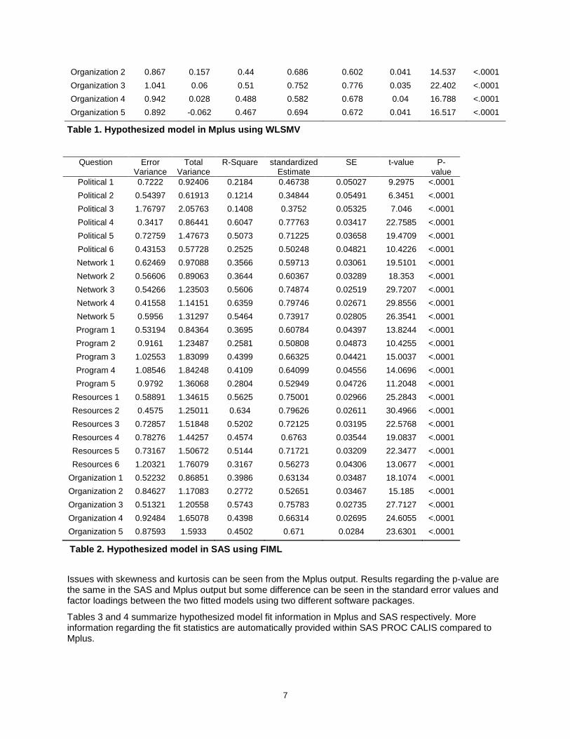
Table 2. Hypothesized model in SAS using FIML

Issues with skewness and kurtosis can be seen from the Mplus output. Results regarding the p-value are the same in the SAS and Mplus output but some difference can be seen in the standard error values and factor loadings between the two fitted models using two different software packages.

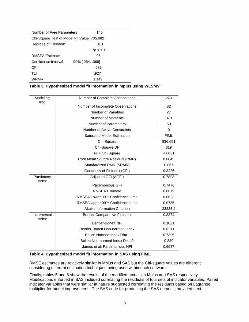
Tables 3 and 4 summarize hypothesized model fit information in Mplus and SAS respectively. More information regarding the fit statistics are automatically provided within SAS PROC CALIS compared to Mplus.

8

Number of Free Parameters 146

Chi-Square Test of Model Fit Value 705.082

Degrees of Freedom 313

*p < .01

RMSEA Estimate .06

Confidence Interval 90% [.054, .066]

CFI .935

TLI .927

WRMR 1.149

Table 3. Hypothesized model fit information in Mplus using WLSMV

Modeling Info

Number of Complete Observations 270

Number of Incomplete Observations 82

Number of Variables 27

Number of Moments 378

Number of Parameters 59

Number of Active Constraints 0

Saturated Model Estimation FIML

Chi-Square 836.691

Chi-Square DF 319

Pr > Chi-Square <.0001

Root Mean Square Residual (RMR) 0.0845

Standardized RMR (SRMR) 0.067

Goodness of Fit Index (GFI) 0.8226

Parsimony Index

Adjusted GFI (AGFI) 0.7898

Parsimonious GFI 0.7476

RMSEA Estimate 0.0679

RMSEA Lower 90% Confidence Limit 0.0623

RMSEA Upper 90% Confidence Limit 0.0735

Akaike Information Criterion 23836.4

Incremental Index

Bentler Comparative Fit Index 0.8374

Bentler-Bonett NFI 0.1021

Bentler-Bonett Non-normed Index 0.8211

Bollen Normed Index Rho1 0.7396

Bollen Non-normed Index Delta2 0.839

James et al. Parsimonious NFI 0.6937

Table 4. Hypothesized model fit information in SAS using FIML

RMSE estimates are relatively similar in Mplus and SAS but the Chi-square values are different considering different estimation techniques being used within each software.

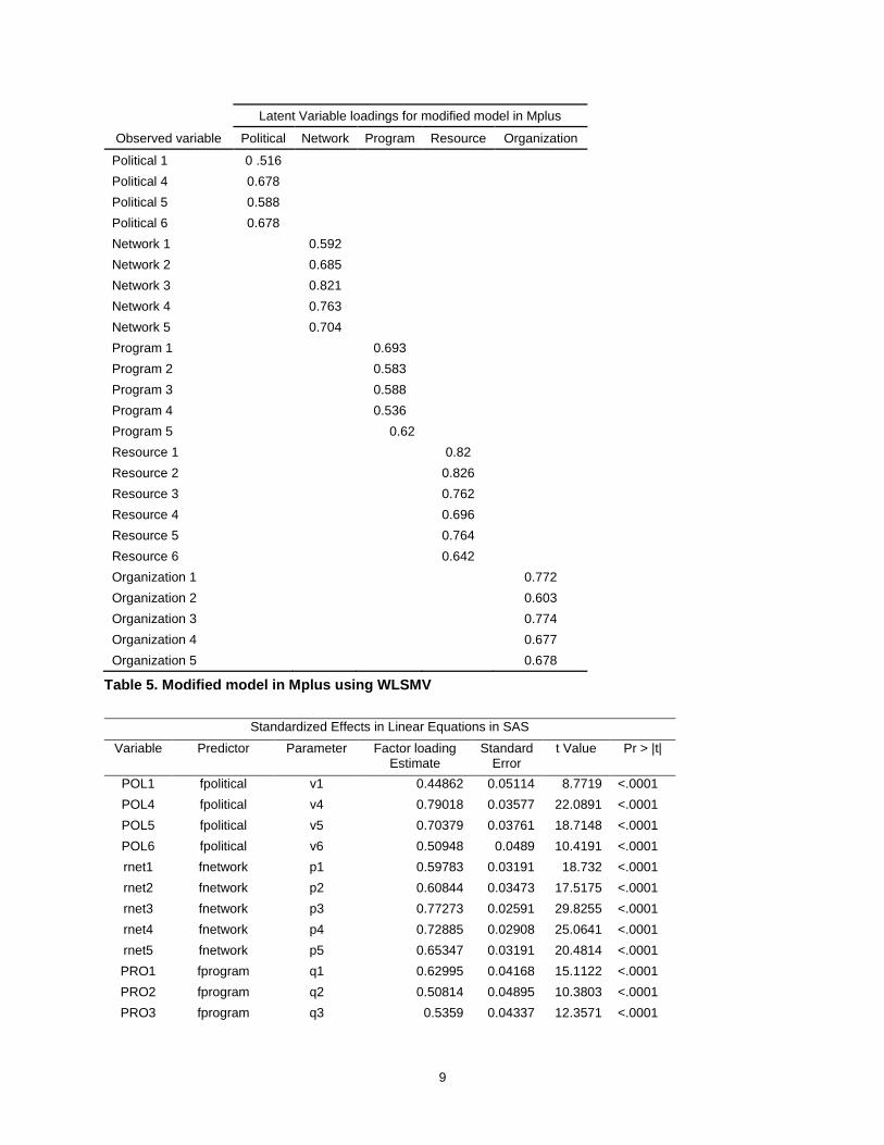
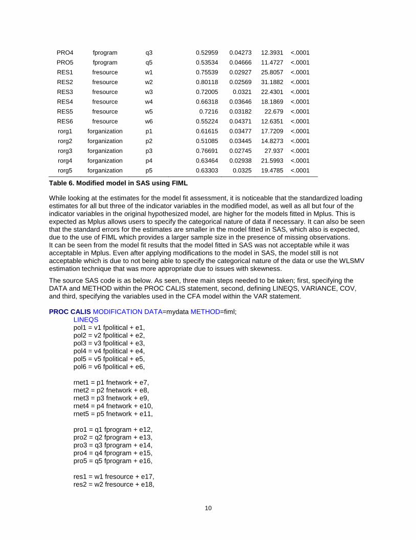
Finally, tables 5 and 6 show the results of the modified models in Mplus and SAS respectively. Modifications enforced in SAS included correlating the residuals of four sets of indicator variables. Paired indicator variables that were similar in nature suggested correlating the residuals based on Lagrange multiplier for model improvement. The SAS code for producing the SAS output is provided next.

9

Latent Variable loadings for modified model in Mplus

Observed variable Political Network Program Resource Organization

Political 1 0 .516 Political 4 0.678 Political 5 0.588 Political 6 0.678 Network 1 0.592 Network 2 0.685 Network 3 0.821 Network 4 0.763 Network 5 0.704 Program 1 0.693 Program 2 0.583 Program 3 0.588 Program 4 0.536 Program 5 0.62 Resource 1 0.82 Resource 2 0.826 Resource 3 0.762 Resource 4 0.696 Resource 5 0.764 Resource 6 0.642 Organization 1 0.772

Organization 2 0.603

Organization 3 0.774

Organization 4 0.677

Organization 5 0.678

Table 5. Modified model in Mplus using WLSMV

Standardized Effects in Linear Equations in SAS

Variable Predictor Parameter Factor loading Estimate

Standard Error

t Value Pr > |t|

POL1 fpolitical v1 0.44862 0.05114 8.7719 <.0001

POL4 fpolitical v4 0.79018 0.03577 22.0891 <.0001

POL5 fpolitical v5 0.70379 0.03761 18.7148 <.0001

POL6 fpolitical v6 0.50948 0.0489 10.4191 <.0001

rnet1 fnetwork p1 0.59783 0.03191 18.732 <.0001

rnet2 fnetwork p2 0.60844 0.03473 17.5175 <.0001

rnet3 fnetwork p3 0.77273 0.02591 29.8255 <.0001

rnet4 fnetwork p4 0.72885 0.02908 25.0641 <.0001

rnet5 fnetwork p5 0.65347 0.03191 20.4814 <.0001

PRO1 fprogram q1 0.62995 0.04168 15.1122 <.0001

PRO2 fprogram q2 0.50814 0.04895 10.3803 <.0001

PRO3 fprogram q3 0.5359 0.04337 12.3571 <.0001

10

PRO4 fprogram q3 0.52959 0.04273 12.3931 <.0001

PRO5 fprogram q5 0.53534 0.04666 11.4727 <.0001

RES1 fresource w1 0.75539 0.02927 25.8057 <.0001

RES2 fresource w2 0.80118 0.02569 31.1882 <.0001

RES3 fresource w3 0.72005 0.0321 22.4301 <.0001

RES4 fresource w4 0.66318 0.03646 18.1869 <.0001

RES5 fresource w5 0.7216 0.03182 22.679 <.0001

RES6 fresource w6 0.55224 0.04371 12.6351 <.0001

rorg1 forganization p1 0.61615 0.03477 17.7209 <.0001

rorg2 forganization p2 0.51085 0.03445 14.8273 <.0001

rorg3 forganization p3 0.76691 0.02745 27.937 <.0001

rorg4 forganization p4 0.63464 0.02938 21.5993 <.0001

rorg5 forganization p5 0.63303 0.0325 19.4785 <.0001

Table 6. Modified model in SAS using FIML

While looking at the estimates for the model fit assessment, it is noticeable that the standardized loading estimates for all but three of the indicator variables in the modified model, as well as all but four of the indicator variables in the original hypothesized model, are higher for the models fitted in Mplus. This is expected as Mplus allows users to specify the categorical nature of data if necessary. It can also be seen that the standard errors for the estimates are smaller in the model fitted in SAS, which also is expected, due to the use of FIML which provides a larger sample size in the presence of missing observations. It can be seen from the model fit results that the model fitted in SAS was not acceptable while it was acceptable in Mplus. Even after applying modifications to the model in SAS, the model still is not acceptable which is due to not being able to specify the categorical nature of the data or use the WLSMV estimation technique that was more appropriate due to issues with skewness.

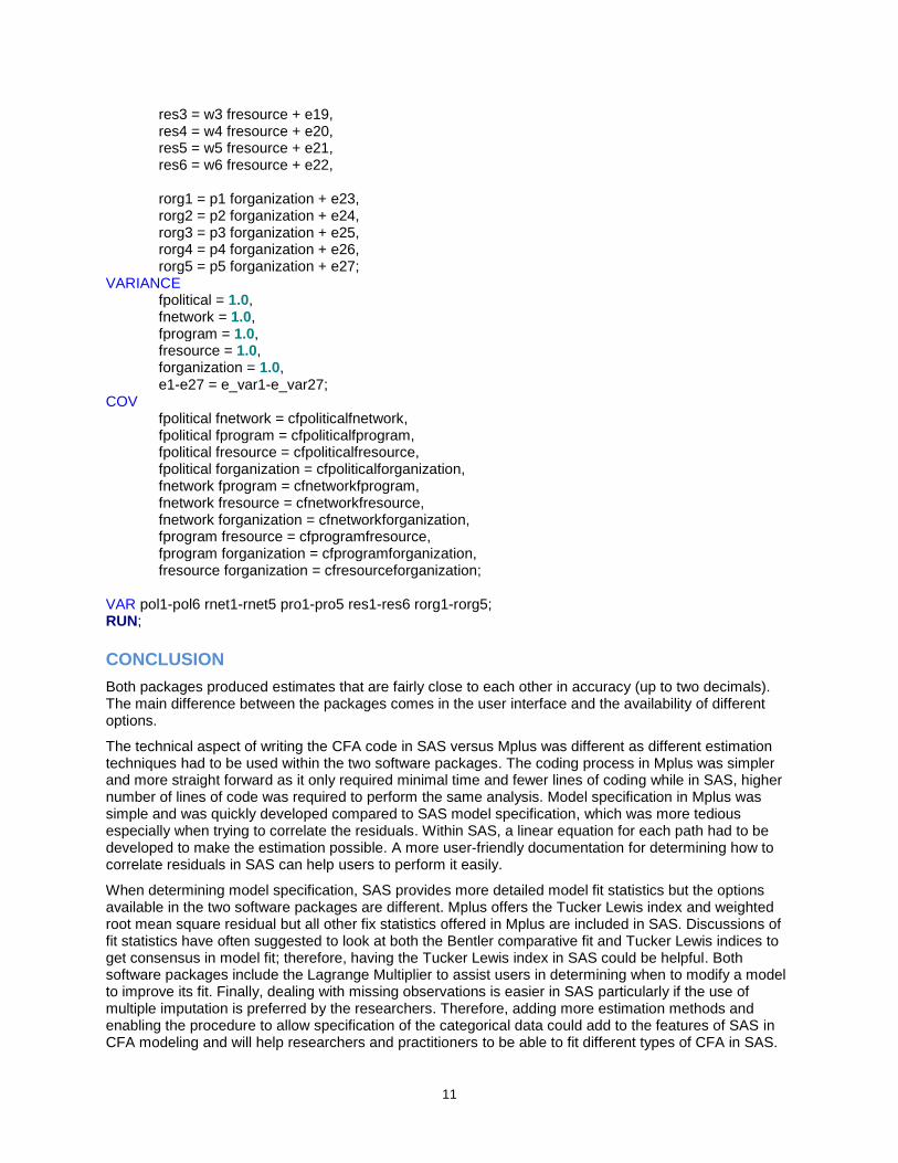
The source SAS code is as below. As seen, three main steps needed to be taken; first, specifying the DATA and METHOD within the PROC CALIS statement, second, defining LINEQS, VARIANCE, COV, and third, specifying the variables used in the CFA model within the VAR statement.

PROC CALIS MODIFICATION DATA=mydata METHOD=fiml; LINEQS pol1 = v1 fpolitical + e1, pol2 = v2 fpolitical + e2, pol3 = v3 fpolitical + e3, pol4 = v4 fpolitical + e4, pol5 = v5 fpolitical + e5, pol6 = v6 fpolitical + e6, rnet1 = p1 fnetwork + e7, rnet2 = p2 fnetwork + e8, rnet3 = p3 fnetwork + e9, rnet4 = p4 fnetwork + e10, rnet5 = p5 fnetwork + e11, pro1 = q1 fprogram + e12, pro2 = q2 fprogram + e13, pro3 = q3 fprogram + e14, pro4 = q4 fprogram + e15, pro5 = q5 fprogram + e16, res1 = w1 fresource + e17, res2 = w2 fresource + e18,

11

res3 = w3 fresource + e19, res4 = w4 fresource + e20, res5 = w5 fresource + e21, res6 = w6 fresource + e22, rorg1 = p1 forganization + e23, rorg2 = p2 forganization + e24, rorg3 = p3 forganization + e25, rorg4 = p4 forganization + e26, rorg5 = p5 forganization + e27;

VARIANCE fpolitical = 1.0, fnetwork = 1.0, fprogram = 1.0, fresource = 1.0, forganization = 1.0, e1-e27 = e_var1-e_var27;

COV fpolitical fnetwork = cfpoliticalfnetwork, fpolitical fprogram = cfpoliticalfprogram,

fpolitical fresource = cfpoliticalfresource, fpolitical forganization = cfpoliticalforganization, fnetwork fprogram = cfnetworkfprogram, fnetwork fresource = cfnetworkfresource, fnetwork forganization = cfnetworkforganization, fprogram fresource = cfprogramfresource, fprogram forganization = cfprogramforganization, fresource forganization = cfresourceforganization;

VAR pol1-pol6 rnet1-rnet5 pro1-pro5 res1-res6 rorg1-rorg5; RUN;

CONCLUSION

Both packages produced estimates that are fairly close to each other in accuracy (up to two decimals). The main difference between the packages comes in the user interface and the availability of different options.

The technical aspect of writing the CFA code in SAS versus Mplus was different as different estimation techniques had to be used within the two software packages. The coding process in Mplus was simpler and more straight forward as it only required minimal time and fewer lines of coding while in SAS, higher number of lines of code was required to perform the same analysis. Model specification in Mplus was simple and was quickly developed compared to SAS model specification, which was more tedious especially when trying to correlate the residuals. Within SAS, a linear equation for each path had to be developed to make the estimation possible. A more user-friendly documentation for determining how to correlate residuals in SAS can help users to perform it easily.

When determining model specification, SAS provides more detailed model fit statistics but the options available in the two software packages are different. Mplus offers the Tucker Lewis index and weighted root mean square residual but all other fix statistics offered in Mplus are included in SAS. Discussions of fit statistics have often suggested to look at both the Bentler comparative fit and Tucker Lewis indices to get consensus in model fit; therefore, having the Tucker Lewis index in SAS could be helpful. Both software packages include the Lagrange Multiplier to assist users in determining when to modify a model to improve its fit. Finally, dealing with missing observations is easier in SAS particularly if the use of multiple imputation is preferred by the researchers. Therefore, adding more estimation methods and enabling the procedure to allow specification of the categorical data could add to the features of SAS in CFA modeling and will help researchers and practitioners to be able to fit different types of CFA in SAS.

12

REFERENCES

Asparouhov, T., & Muthén, B. (2010). Weighted least squares estimation with missing data.

Mplus Technical Appendix, 1-10. Bentler, P. M. (1990). Comparative fit indexes in structural models. Psychological Bulletin, 107(2), 238. Bollen & J. Long (Eds.), Testing Structural Equation Models (pp. 136–162). Newbury Park, CA: Sage. Boris, E. T. & Roeger, K. L. (2010). Grassroots civil society: The scope and dimensions of small public

charities. Charting Civil Society: A series by the Center on Nonprofits and Philanthropy. 24, 1-7. Browne, M. W., & Cudeck, R. (1993). Alternative ways of assessing model fit. Sage focus editions, 154,

136-136. Carmines, Edward G., and Richard A. Zeller (1979). Reliability and Validity Assessment. Newbury Park,

CA: Sage Publications DiStefano, C., Zhu, M., & Mindrila, D. (2009). Understanding and using factor scores: Considerations for

the applied researcher. Practical Assessment, Research & Evaluation, 14(20), 1-11. Fredericksen, P., & London, R. (2000). Disconnect in the hollow state: the pivotal role of organizational

capacity in community‐based development organizations. Public Administration Review, 60(3), 230-239.

Hu, L., & Bentler, P. M. (1999). Cutoff criteria for fit indexes in covariance structure analysis: Conventional criteria versus new alternatives. Structural Equation Modeling: A Multidisciplinary Journal, 6(1), 1–55. https://doi.org/10.1080/10705519909540118

Kline, R. B., & Santor, D. A. (1999). Principles & practice of structural equation modelling. Canadian Psychology, 40(4), 381.

Muthén, B. O. (1998–2004). Mplus Technical Appendices. Los Angeles, CA: Muthén & Muthén. Muthen, L. K., and Muthen, B. O. (1998–2010), Mplus User’s Guide (6th ed.), Los Angeles, CA: Muthen &

Muthen. Narayanan, A. (2012). A review of eight software packages for structural equation modeling. The

American Statistician, 66(2), 129-138.

Rubin, H. J. (2000). Renewing hope within neighborhoods of despair: The community-based development model. SUNY Press.

Salamon, L. M. (Ed.). (2002). The tools of government: A guide to the new governance. Oxford University Press.

Schill, M. H. (1996). Assessing the role of community development corporations in inner city economic development. New York University Review & Social Change, 22, 753-776.

Schreiber, J. B., Nora, A., Stage, F. K., Barlow, E. A., & King, J. (2006). Reporting structural equation modeling and confirmatory factor analysis results: A review. The Journal of educational research, 99(6), 323-338.

Steiger, J. H. (2007). Understanding the limitations of global fit assessment in structural equation modeling. Personality and Individual Differences, 42(5), 893–898.

Tucker, L. R., & Lewis, C. (1973). A reliability coefficient for maximum likelihood factor analysis. Psychometrika, 38(1), 1-10.

Vidal, A. C., Freiberg, S., Otchere-Agyei, E., Saunders, M. (1999). Faith-based organizations in community development. Urban Institute.

Yu, C. 2002. Evaluating cutoff criteria of model fit indices for latent variable models with binary and continuous outcomes. (Doctoral dissertation).

13

ACKNOWLEDGMENTS

We would like to thank Dr. Nathaniel S. Wright from Texas Tech University for developing the CBCBS instrument and sharing his data with us for this study. We also appreciate the efforts of Lauren Matheny, Connie Couch, and Justin Harding in evaluating the CBCBS survey.

CONTACT INFORMATION

Your comments and questions are valued and encouraged. Contact the author at:

Niloofar Ramezani, Ph.D. nramezan@gmu.edu Kevin Gittner, M.S. M.B.A. Kevin.gittner@unco.edu

SAS and all other SAS Institute Inc. product or service names are registered trademarks or trademarks of SAS Institute Inc. in the USA and other countries. ® indicates USA registration.

Other brand and product names are trademarks of their respective companies.