HAL Id: jpa-00210072https://hal.archives-ouvertes.fr/jpa-00210072

Submitted on 1 Jan 1985

HAL is a multi-disciplinary open accessarchive for the deposit and dissemination of sci-entific research documents, whether they are pub-lished or not. The documents may come fromteaching and research institutions in France orabroad, or from public or private research centers.

L’archive ouverte pluridisciplinaire HAL, estdestinée au dépôt et à la diffusion de documentsscientifiques de niveau recherche, publiés ou non,émanant des établissements d’enseignement et derecherche français ou étrangers, des laboratoirespublics ou privés.

Configuration space analysis of travelling salesmanproblems

S. Kirkpatrick, G. Toulouse

To cite this version:S. Kirkpatrick, G. Toulouse. Configuration space analysis of travelling salesman problems. Journalde Physique, 1985, 46 (8), pp.1277-1292. <10.1051/jphys:019850046080127700>. <jpa-00210072>

1277

Configuration space analysis of travelling salesman problems

S. Kirkpatrick

IBM T. J. Watson Research Center, Yorktown Heights, N.Y. 10598, U.S.A.

and G. Toulouse (*)

Laboratoire de Physique de l’E.N.S., 24, rue Lhomond, 75231 Paris Cedex 05, France

(Rep le 14 février 1985, accepté le 18 avril 1985)

Résumé. 2014 Le problème du voyageur de commerce (TSP) et le modèle d’Ising d’un verre de spin sont, respective-ment, des archétypes pour les problèmes d’optimisation combinatoire en informatique et pour les systèmes désor-donnés frustrés en physique de la matière condensée. Il a été suggéré récemment que ces deux domaines ont beau-coup de phénomènes en commun. Pour voir si, de fait, les problèmes d’optimisation combinatoire peuvent êtredes verres de spin, nous définissons un TSP à distance aléatoire aussi semblable que possible au modèle idéalisé,à portée infinie, des verres de spin. A la lumière des résultats récents pour les verres de spin, nous analysons lesobservables thermodynamiques et les corrélations internes entre configurations localement stables. L’hypothèsed’un gel dû à la frustration et d’une structure hiérarchique ultramétrique dans l’espace des configurations estsolidement argumentée, pour ce problème de voyageur de commerce.

Abstract 2014 The travelling salesman problem (TSP) and the Ising model of a spin glass are archetypes, respectively,of the combinatorial optimization problems of computer science and of the frustrated disordered systems studiedin condensed matter physics. It has recently been proposed that these two fields have many phenomena in common.To see if, in fact, combinatorial optimization problems may be spin glasses, we define a random distance TSP assimilar as possible to the idealized infinite-ranged model of spin glasses. Thermodynamic observables and internalcorrelations among locally stable configurations are analysed in the light of recent results for spin glasses. Evidencefor freezing due to frustration and for a hierarchical, ultrametric structure of configuration space in this TSP ispresented.

J. Physique 46 (1985) 1277-1292 Ao8T 1985,

ClassificationPhysics Abstracts05.20 - 75.50 - 85.40

The travelling salesman problem (TSP) is oneclassic example of a complex optimization problem.Easy to formulate, it is yet hard to solve : it belongsto the class of NP-complete problems [1]. Recently,the use of simulated annealing, a stochastic algorithmbased on the Monte Carlo method (as developed inthe context of the statistical physics of disorderedsystems, e.g. spin glasses), was advocated as an

appropriate algorithm for approximate solution ofcomplex optimization problems [2]. The applicationof the simulated annealing method to TSP has alreadybeen discussed to some extent [2, 8].

There are good reasons why spin glasses providea suggestive model for complex optimization pro-blems [2]. They possess, in a clear way, the physicalingredients of frustration and disorder, which leadto a large number of locally minimal solutions andto freezing phenomena. The simulated annealingmethod addresses the problem of getting stuck in alocal minimum by allowing for uphill moves.

Meanwhile, new advances in the theory of spinglasses have directed attention toward the distribu-tion of local minima in the landscape of configurationspace. Some sharp results have been obtained forlong range Ising spin glasses : ultrametricity, non-reproducibility, loss of self averaging [9, 10, 23].Several new concepts and tools have thus been created.

Article published online by EDP Sciences and available at http://dx.doi.org/10.1051/jphys:019850046080127700

1278

The notion of configuration space landscape is

obviously so general as to be of interest in manyproblems. This paper is a study, largely numerical,of the characteristics of configuration space landscapesfor a random distance version of the TSP.

Section 1 describes the problem and our analysis.Section 2 presents the numerical data.Section 3 surveys the recent relevant results obtained

in the theory of spin glasses, and draws some compa-risons with our TSP data.Some general views can be extracted from these

case studies. The analysis of configuration spacelandscapes aims at finding a more detailed and morephysical categorization among complex optimizationproblems. Numerical and analytical strategies for

solving such problems will thus be based on sounderphysical grounds. (Present problem classifications,based on worst case analysis of algorithmic complexity,are often very broad, so for instance the problem offinding the ground state of a ferromagnet might beconsidered NP-complete because it is lumped togetherwith the spin glass problem.)

Finally, in section 4, we discuss the impact of theseideas on the monitoring of the change of configurationspace landscapes in memory models, under learningand unlearning processes.

1. Introductory analysis.

The travelling salesman problem (TSP) is simplystated. A list of N cities and a means of obtainingthe distance between any pair of cities is given. Theobjective is to find a tour, or permutation, P, of thecities such that the total length L, of travel through allcities and returning to the first one in the order P :

is minimized. Since the starting point and directionof the tour do not matter, there are (N - 1) !/2 distincttours. Heuristic strategies which search for near-

optimal tours will be able to explore only a tinyfraction of this enormous configuration space if Nis large.

S. Lin [11] has introduced a natural rearrangementof a given tour which permits efficient search. Twosteps on the tour are discarded, say di,i+ 1 and dj,j+ 1.are replaced by d,,j and di+ 1,j+ 1 so that the newpatnis again a tour. There are N(N - 1)/2 suchmoves from any tour.

« Iterative improvement », or exhaustive search

using this class of moves until no further improve-ments can be found, is a powerful way of improvingupon an initial guess of a reasonable tour. Several

groups have recently [2-7] used the Metropolisalgorithm to enhance the effectiveness of search withthese moves. In general they find solutions with

annealing and Lin’s 2-bond moves which are as good

as can be found with exhaustive search using replace-ment of 3 or more bonds.The 2-bond moves impose a natural topology

on the configuration space, giving each tour 0(N 2 )neighbours. A tour which is shorter than all of its

neighbours is termed « 2-optimal » or 2-opt. This isnot the only possible notion of neighbourhood. Forinstance, Cemy [4], Lundy [6], and Kirkpatrick (unpu-blished) have attempted searches using the N inter-changes of successive cities on the tour or the N 2interchanges of any pair of cities, but these movesusually turn short configurations into long ones, anddo not lead to effective searches.A fast, but more limited method of sampling the

configuration space should also be mentioned. Calleda « greedy algorithm &#x3E;&#x3E; because it has finished in

only N steps it is a useful means of obtaining trialconfigurations. One picks one city at random, takesthe closest city as the second step, the closest remain-ing city as the third, and so on until the tour is complete.This differs from an iterative search in that at most N

configurations can be constructed (in practice, fewerthan N distinct tours are usually found).The nature of the distances dij has a big influence

on the difficulty of the TSP. In practical problems thedij may be calculated in an appropriate metric fromthe positions of the N cities, or they may be tabulatedquantities, representing some more complicated cost.For N points randomly distributed in a d-dimensionalEuclidean unit cube, Beardwood et al. [12] haveshown that the minimal tour length is proportionalto N times the expected nearest neighbour distance,N - Ild In this case, all the heuristics discussed approachthe exact limit and give expected outcomes propor-tional to N(I - Ild). The greedy algorithm gives confi-gurations 20 percent longer than optimal in some 2-dimensional problems [2] (KGV), while the otherheuristics are within a few percent of each other.

In this paper we shall consider a simple but arti-ficial TSP in which the distances are symmetric(d; = dji) random variables independently drawnfrom the uniform distribution over the interval (0, 1).

This model is appealing for its simplicity and free-dom from geometry. We hope that it may eventuallyprove, as has the S. K. model of spin glasses [13],to be analytically tractable and provide a « meanheld » limit of the statistical mechanics of a travellingsalesman. However, Vannimenus and Mézard [14]have pointed out that the uniform distribution is notthe infinite dimensional limit of the distribution ofdistances between points placed at random in a finited-dimensional volume. Still, there is inherent simpli-city in the uniform distribution which explains ourchoice.The expected nearest neighbour distance is the

smallest of (N - 1) random numbers in (0, 1), hence0 (N -1 ), in this model. Thus an N-step tour must beat least 1 unit long, and may, as an extension of theBeardwood result, have expected length tending to

1279

be constant 0(1) as N - oo, but we know of no proofof this. The greedy algorithm for this random distanceproblem gives expected length

and provides an upper bound.In figure 1 we display tour lengths obtained for

this random distance TSP by exhaustive 2-opt and3-opt searches, and by simulated annealing basedon 2-bond and limited 3-bond moves. This problemis difficult enough to discriminate asymptoticallybetween different heuristics. As with 2-dimensionalTSP’s, it was found that simulated annealing with 2-bond moves gave answers as good as exhaustivesearch with 3-bond moves for comparable comput-ing times. In figure 1, the annealing schedule wasadjusted so that the computing time for the annealedruns was kept O(N 2) . Thus, exhaustive 3-opt, withcomputing time aN 3, became better than 2-bondannealing for large N. For N &#x3E; 100, it was extremelycostly to obtain good configurations by any heurisic :for N 50, the solutions appear to be close to thepresumed optima.

I

Fig. 1. z Optimal tour length for random distance TSP’sof up to N = 400 sites, as obtained by various algorithms.The dashed line is the upper bound provided by the greedyalgorithm. The solid points are from iterative improvementusing exhaustive search for 2-bond rearrangements (squares)and 3-bond rearrangements (dots). The open points for

N &#x3E; 24 are simulated annealing results using 2-bondmoves (squares) and three bond moves (circles). The opendata for N 12 are exact results.

Some simple calculations will suffice to sketch inthe important energies (i.e. lengths) and temperaturesof the random distance TSP, viewed as a statisticalmechanics problem. At high temperatures we neglectthe fact that the configuration must be a tour andsimply treat each bond as contributing with a Boltz-mann weight. This corresponds to the « annealed »rather than « quenched &#x3E;&#x3E; approximation used indisordered systems. It is known to give a useful des-cription of spin glasses above freezing, and wasapplied in an independent study by Bonomi andLutton [5] to describe a TSP in 2D at non-zero

temperature.The statistical mechanics of this « annealed &#x3E;&#x3E;

approximation follows simply from treating eachof the N bonds as independent. The partition func-tion, Z, is approximated by

where

and

The path length per bond, I(fl) = L/N, is obtained by

This has limits I - 1/2 at high temperature andI - T at low temperature, with a crossover aroundP - 1. But, since I ~ N -1 is the smallest possiblefor actual tours, the annealed theory will have brokendown for P ~ N.The length per bond, I(P), plays the role of internal

energy in the TSP, so the specific heat, C(P), is obtainedby

which has limits

and

The entropy, S, can be obtained by integrating C/T,or by defining a free energy, F,

Now the entropy per step of the tour is given by

1280

with the result

At high temperatures,

and at low temperatures,

This negative entropy catastrophe is familar fromclassical statistical mechanics. Since negative entropyis unacceptable for a problem with discrete states,it gives a strong limit for the validity of the annealedmodel,

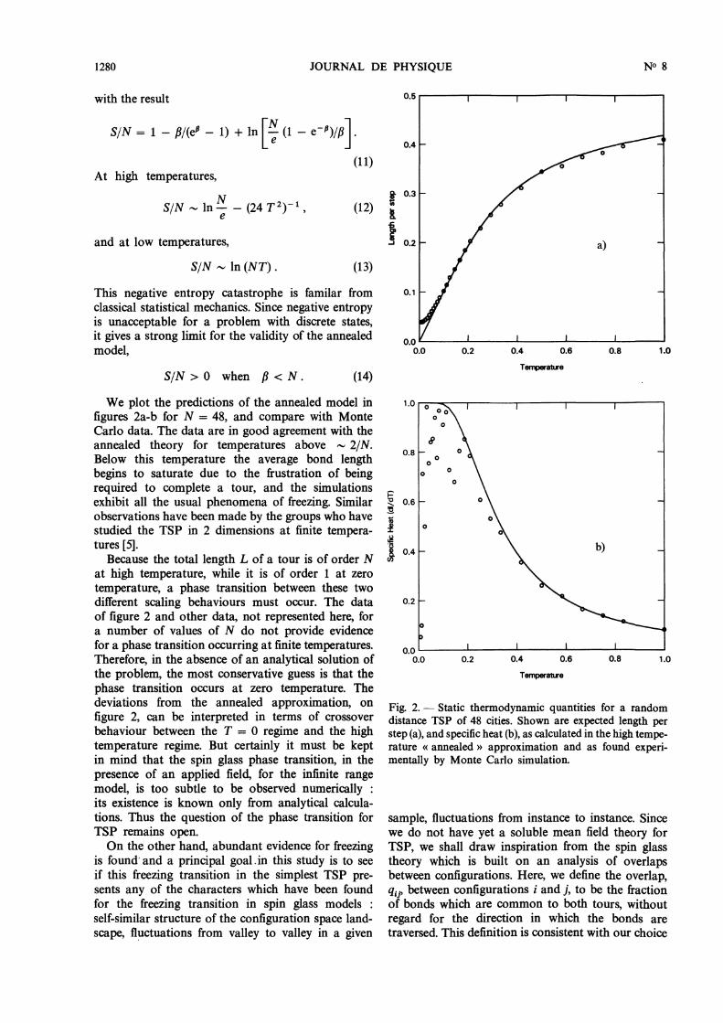
We plot the predictions of the annealed model infigures 2a-b for N = 48, and compare with MonteCarlo data. The data are in good agreement with theannealed theory for temperatures above - 2/N.Below this temperature the average bond lengthbegins to saturate due to the frustration of beingrequired to complete a tour, and the simulationsexhibit all the usual phenomena of freezing. Similarobservations have been made by the groups who havestudied the TSP in 2 dimensions at finite tempera-tures [5].

Because the total length L of a tour is of order Nat high temperature, while it is of order 1 at zero

temperature, a phase transition between these twodifferent scaling behaviours must occur. The dataof figure 2 and other data, not represented here, fora number of values of N do not provide evidencefor a phase transition occurring at finite temperatures.Therefore, in the absence of an analytical solution ofthe problem, the most conservative guess is that thephase transition occurs at zero temperature. Thedeviations from the annealed approximation, on

figure 2, can be interpreted in terms of crossoverbehaviour between the T = 0 regime and the hightemperature regime. But certainly it must be keptin mind that the spin glass phase transition, in thepresence of an applied field, for the infinite rangemodel, is too subtle to be observed numerically :its existence is known only from analytical calcula-tions. Thus the question of the phase transition forTSP remains open.On the other hand, abundant evidence for freezing

is found and a principal goal. in this study is to seeif this freezing transition in the simplest TSP pre-sents any of the characters which have been foundfor the freezing transition in spin glass models :self-similar structure of the configuration space land-scape, fluctuations from valley to valley in a given

Fig. 2. - Static thermodynamic quantities for a randomdistance TSP of 48 cities. Shown are expected length perstep (a), and specific heat (b), as calculated in the high tempe-rature « annealed &#x3E;&#x3E; approximation and as found experi-mentally by Monte Carlo simulation.

sample, fluctuations from instance to instance. Sincewe do not have yet a soluble mean field theory forTSP, we shall draw inspiration from the spin glasstheory which is built on an analysis of overlapsbetween configurations. Here, we define the overlap,q; ., between configurations i and j, to be the fractionof bonds which are common to both tours, withoutregard for the direction in which the bonds are

traversed. This definition is consistent with our choice

1281

of 2-bond moves to generate a topology in the confi-guration space since it implies that two configurationsare close when only a few such moves are appliedto the first to generate the second.Some annealed results are of interest in thinking

about the overlap of tours. Two randomly selectedtours of N cities will have, on average, 2 bonds incommon, and the distribution, P(q), of overlaps isPoisson in the limit of large N [15].

If we include the effect of temperature as in theprevious discussion, we find the expected overlapis given by

for pairs of tours, weighted by their equilibrium pro-bability of occurrence.For p tours, the comparable expression is

From (17) we see that little overlap is expected whenfl = 1.0, and significant overlap once fl = N, wherewe have shown the annealed theory is inadequate.At low temperatures, when there is significant

overlap between tours, we would like to know moreabout the bonds which participate in large numbersof tours. Questions like how frequently a given bondappears in the sample, or how many bonds take partin a given class of locally optimal states are of interest.For a set { a } of M tours (for example, all of the

2-opt configurations), define

Then

is the number of occurrences of the i-th bond. Itsrelative frequency f --_ NiM. The overlap between ptours, Qal’"’’ap can be expressed as

so

Thus the frequency of bond occurrence can be usedto generate higher order overlap statistics.Now if we introduce a frequency distribution, p( f ),

normalized such that

the identity

gives a useful sum rule on p( f ) :

We show numerical evidence in the following sec-tion that for the set of 2-opt configurations, p( f )consists of a nearly constant piece plus a delta func-tion at f = 0, representing the bonds which neverparticipate. Introducing an ansatz, po( f ), for the

density with this two-part form :

we find from (25) that A = (2 - y) N and as a resultthe number of bonds which participate in the sample

of M configurations will be N. This form for

po(f) implies that only a finite number of bonds percity participate in the locally stable solutions of aTSP, a hypothesis which suggests intriguing heuristicsfor restricting the search for an optimal solution ofthe TSP.

There are additional quantities of interest in

studying TSP, but since we have no theoreticalestimates these will be introduced below, during thediscussion of the numerical data.

2. Numerical results.

The numerical work in this paper is based uponpopulations of distinct locally minimal tours whichwere extracted from several samples of the randomdistance TSP in each of three sizes : N = 12, 24, and48. Exact enumeration was employed to study toursof 12 cities. Monte Carlo methods were required forN = 24 and above. TSP’s with N = 96 were alsostudied but are not reported because the tours obtain-ed were probably not close to optimal, as figure 1

suggests.Eleven instances, i.e. matrices of random distances

dij, were analysed for N = 12. For each instance, all2-opt configurations were extracted and saved in adisk file. There are approximately 4 x 10’ distincttours of length 12. Generating all tours and calcu-lating their lengths required about 4 min on anIBM 3081. We used an algorithm due to Trotter [16] togenerate permutations by N ! successive interchangesof adjacent elements. Trotter’s algorithm appears to beoptimal for our purposes. The 11 minimal tours

obtained ranged in length from 1.16 to 2.47, with amean of 1.83 and variance of 0.44. From 11 to 58 2-opttours were extracted; on average there were 29 perconfiguration. The lengths of the 2-opt tours rangedup to 3.3. The average spread in length of the 2-opt

1282

states for a given instance was 0.9, the variance, 0.4.Since the mean length of a tour for N = 12 in thismodel is 6 and the maximum length 0(12), the 2-opttours are a more restricted class of states than the

locally minimal spin glass configurations, which arefound at energies up to the average energy of a spinconfiguration [17, 18]. A 2-opt solution is stable

against O(N 2) bond rearrangements, while a spinconfiguration with all spins frozen is stable against Nindividual spin reversals. Thus the narrower relativerange of lengths for the 2-opt solutions is not sur-

prising.The 2-opt states were also tested for 3-optimality.

On average, two 3-opt tours per instance were found,with some instances having a unique 3-opt configura-tion and others as many as 4.

To obtain 2-opt tours with N = 24 and 48, asimulated annealing procedure (KGV) was employedto generate 100 2-opt configurations for each instance,heating the system to a temperature of 2 or morebriefly between coolings to provide a random restart.For N = 24, if the samples were cooled slowly, onlya few distinct 2-opt states resulted. Thus a relativelyrapid annealing schedule was developed, which gavean average of 55 distinct 2-opt tours in the set of 100retained for each instance. One or two of the shortest

2-opt tours were generated 10 or more times each,while most of the longer 2-opt tours created wereunique. We found from 3 to 23 of these tours werealso 3-opt, for an average of 11 per instance. The

range of lengths sampled is not relevant for N = 24,since the selection is not exhaustive or random. Thesame annealing schedule was followed in generatingtours for four instances with N = 48, taking four timesas many rearrangement steps at each temperature.Each cooling run terminated only when a 3-optconfiguration was formed, which proved to occurfrequently. The 100 3-opt tours generated for eachinstance were all distinct.Next we show the distribution of pairwise overlaps

found in the sample populations of 2-opt (or 3-opt)tours. Figures 3a-c show similar-looking curves forP(q) with N = 12, 24 and 48, respectively. Curvesfor the different instances at each N are superimposed.In each case the most probable values of q occur atabout 2/3. Note the differences between figures 3a-cand the overlap distributions predicted and found forspin glasses. There P(q) is nonzero down to q = 0;overlaps of negative sign are meaningful betweenspin configurations. The distributions in figures 3do not include self overlap, i.e. terms qij with i = j,and thus are normalized to slightly less than unity.However we prefer to avoid the delta functions thisterm requires and will also leave out self overlapsin the joint distributions explored below.With increased temperature, the tours spread fur-

ther apart in configuration space, reducing the averageoverlap, but the spread in P(q) does not change much.Figure 4a shows distributions, P(q), obtained for one

Fig. 3. - Overlap distributions, P(q), for eleven instancesof N = 12 (a), eight cases of N = 24 (b), and four caseswith N = 48 (c). In figures 3, 4, 9-13, we plot data againstthe integervalued Nq for programming convenience. Thevertical scales are arbitrary ; P(q) is a normalized probabilitydistribution.

1283

Fig. 4. - P(q) for samples annealed to temperatures 1/12,1/24, and 1/48. In (a) random restarts were employed aftereach sample configuration was collected. In (b) the confi-gurations were obtained by Monte Carlo runs at the indicat-ed fixed temperatures, without warming up between samples.See the caption of figure 3 for notations.

instance with N = 48 in populations of 100 toursobtained by repeated cooling from the hot, scrambledstate to various lower temperatures.The effect of the energy landscape which confines

the Monte Carlo search to a particular valley or tothe vicinity of a set of minima is evident in figure 4b.Here we plot P(q) obtained at a similar set of tempera-tures, but this time without randomizing the tourbetween samples. The final set of tours obtained over-lap more strongly, with a most probable value ofq - (7/8), than do the tours found by repeated ran-dom restarts in figure 3c.

We have also studied the bond frequency distribu-tions characterizing the samples of locally optimalconfigurations. The well-behaved experimental quan-tity which is closely related to p( f ) is the cumulativedistribution, D( f ) :

Figures 5a-c plot f as a function of D( f ) for theinstances with 12, 24 and 48 cities, respectively. Theabscissa and ordinate are interchanged for conve-nience in generating these figures, which were createdby sorting the list of all bonds in each instance indecreasing order by frequency, then plotting bondfrequency against that bond’s position in the sortedlist. If p( f ) were constant (y = 0 in the ansatz po),then D( f ) would be a straight line, and only 2 Nbonds would participate in all 2-opt configurations.Furthermore, a constant bond frequency distribu-

tion p(f&#x3E; implies zip&#x3E; = £ , where Qp &#x3E; hasbeen defined in (21), which is in good agreementwith the estimate Q 2 &#x3E; -- 31 z obtained from thedate of figure 3. In fact, figures 5 suggest that p( f ) isroughly constant, with some extra contributions closeto f = 0 and f = 1. About 3 N bonds in eachinstance contribute to our samples of optimal confi-gurations. The distributions shown in figures 5

sharpen up as N increases, with the case N = 48showing little instance-to-instance scatter.

Figure 6, based on the samples used in figure 5c,shows the effect of higher temperature in reducingconfiguration overlap. In figure 6 no bond occurs inall samples, and a larger number of bonds participatein the configurations analysed. This is consistent withthe lower average value of q observed.

It seems of interest to ask whether other sets of

configurations, more easily calculated, would containthe same set of useful bonds as are present in theannealed 3-opt configurations, which are relativelycostly to compute. We consider the set of N

« greedy » solutions to a given TSP obtained bystarting at each city. (In fact, for N = 48, one or twoof the greedy solutions is duplicated, but we did notbother to remove duplicates). The best greedy solutionsfound for N = 48 are about 50 percent longer thanthe best annealed solutions (see Fig. 1). The distribu-tion of bond frequencies for the greedy set of configu-rations, shown in figure 7 for one N = 48 instance, issimilar in shape to the curves of figure 5c, except fora tail extending out to 4N bonds. The rather longbonds taken at the end of a greedy tour, when a fewscattered cities remain to travel between, could accountfor this tail.There are other differences. In figure 8 we plot bond

frequencies against bond length for greedy andannealed configurations of the same TSP. Theannealed solutions consist of bonds with a narrow

1284

Fig. 5. - Bond frequency plotted versus number of bondswhich occur at least that frequently, for : a) N = 12,b) N = 24 and c) N = 48 locally optimal TSP solutions.

Fig. 6. - Cumulative distribution of bond frequencies,as in figure 5, for an N = 48 sample annealed to T = 1/6,then quenched.

1285

Fig. 7. - Cumulative distribution of bond frequencies forall greedy solutions of the same instances of TSP withN = 48 as in figure 5c.

range of lengths, while some of the frequentlyencountered greedy bonds are quite long. Presumably,the rigid greedy strategy for creating a tour forces thesame mistake repeatedly. Nonetheless, of the 60shortest bonds in the annealed sample only threeare not observed in the greedy sample. However,there are 37 bonds out of the 141 distinct bonds in theannealed sample of 100 configurations which werenever generated by the greedy algorithm. Even if weconcentrate on the 5 shortest tours obtained byannealing we find that these employ 76 distinct

bonds, and six of them are not obtained in the greedysample. Three of these six bonds occur in four or moreof the five shortest tours. A sample of 50 tours wasgenerated by cooling to a temperature at which freezingbegins, 1.4/N, using 50 independent random starts.This sample contained 192 distinct bonds, includingall the bonds discovered in the 100 annealed near-opti-mal configurations.Next we shall analyse the data for evidence of the

ultrametric structure known to exist in spin glasses.In a Euclidean space, the triangular inequality

says that any side of a triangle is smaller or equal tothe sum of the other two :

An ultrametric space is defined by a stronger inequa-lity, the ultrametric inequality :

This implies that any triangle is either isosceles withsmall basis, or equilateral. Obviously, the precedinginequalities can be expressed in terms of overlaps,

Fig. 8. - Relative bond frequencies plotted against bondlength for 100 3-opt solutions (circles) and all greedysolutions (crosses) of an N = 48 TSP.

rather than distances. The ultrametric inequality wasfirst put forward by M. Krasner, around 1930, in thecontext of arithmetics [19]. Notions of ultrametricityhave also been used in the classification of data invarious sciences, and especially in biological taxo-nomy [20]. There are various ways to define overlapsor distances between two biological objects, accordingto the characteristics that are under study. If the dis-tance matrix of a collection of biological objects isultrametric, then there is a unique, well defined, evo-lution tree such that the distance between two objectsis determined by the closest common ancestor (theolder the bifurcation the larger the evolved divergence,and thus the distance). In the general case, where thedistance matrix is not purely ultrametric, biologistsstill wish to reconstitute an evolution tree. The two

simplest procedures to do so are called « single linkagesclustering » and « complete linkage clustering » [21].In both procedures, the distance matrix is modifiedsystematically to become ultrametric, with as fewmodifications as possible. In the first procedure, alldistances are either decreased or unmodified, and thesolution is unique. In the second procedure, distancesare either increased or unmodified, and the solutionneed not be unique. So, these procedures somehowbracket the problem between ultrametric upper andlower bounds. If the evolution trees so obtained are

analogous, this is an indication that the problempossessed a strong underlying ultrametric structure.If not, one has to resort to less stringent and moreQuantitative ultrametricity tests.

The triangle inequality (27) takes a slightly differentform when the variables considered are overlaps,not distances. If we know that tours 1 and 2 differ in

1286

only N(1 - q12) of their bonds, and calculate overlapsq13 and q23 to a third state, then the maximum diffe-rence between q13 and q23 is

The most direct check for ultrametric statistics isthe distribution of the number of triangles(q12’ q23’ q 13) as a function of the lengths of the longerlegs q23 and q13. The triangle inequality may imposesevere constraints on this plot. For example, see

figure 9a, for N = 24, Nql2 = 21, where the resultingdistribution is cut off at N q13 - q23 1 = 4. Part ofthe peaking in figure 9a is due to the narrow range ofP(q). We subtract the uncorrelated backgroundP(q13) P(q23) from the data in figure 9a to remove thiseffect, and show the result as figure 9b. While theremoval of background leaves the ridge narrower andstill rather high the negative contribution on eitherside of the ridge in figure 9b is deepest at the triangleconstraint value N q13 - q23 I = 4. For this reason,plots of the statistics of triangles are not informativeabout N = 12.

Fig. 9. - Distribution of triples of overlaps qij qjk qki forN = 24 for which the largest overlap is 21 bonds. In (a) isshown the raw data. In (b) the uncorrelated backgroundis subtracted out. Vertical scales are arbitrary. The twohorizontal variables are overlaps.

The triangle data is not as compromised for thecase N = 48. Data for Nql2 = 33, the most probablevalue of q, are plotted with the uncorrelated back-ground subtracted out in figure 10a. The restrictionN I q13 - q 2 3 1 ’-- 15 does not affect the region shown.Subtracting the background to obtain figure l0areduces the peak height by a factor of almost 12, andreduces the width of the ridge from about ± 10 to+ 3. If we choose Nql2 = 39, at the high end of theobserved distribution of overlaps, the triangle statisticsagain form a ridge with steep sides at ± 3-4 bonds.The subtracted data shown in figures lOb and 10c has

Fig. 10. - Subtracted statistics of all triangles formedamong 3-opt tours of N = 48 cities with Nqmax = 33 (a)and 39 (b, c). Vertical scales are arbitrary.

1287

a peak height which represents about half of theuncorrected data. Both front and back views (fromNql3 - Nq23 = 39 looking to small q, and from

Nql3 - Nq23 = 21 looking to large q) are provided,since the negative density due to subtracting the back-ground is largest in the middle of the surface plotted.The correlation that emerges in these plots is sensitiveevidence for an ultrametric structure, and may be usedfor quantitative comparison with results in othermodels.

By integrating over the length of one side, qik, weobtain P(qip q;k) - P(qij) P(qk) and collapse all our

data onto a single plot for each value of N, eliminatingthe distraction of the triangle inequality. In figures 1 la-fare displayed the results of this compression of thedata for N = 12, 24 and 48. Both front views (downthe qij = qjk axis) and side views (both qij and zincrease to the right) are shown. The distributions infigure 11 have a characteristic two-peaked form for allthree problem sizes, and stay roughly constant inwidth as N increases. The upper peak has a greaterwidth transverse to the ridge line than the lower peak,but this difference becomes less prominent as N

increases.

Fig. 11. - Subtracted statistics of pairs of bonds, for N = 12(a, b), N = 24(c, d), and N = 48(e, f). Figures lla, c and eshow the data looking along the qij = qik axis from the large q end. Figures llb, d and f show the same cases from the side.Vertical scales are arbitrary.

1288

If instead of integrating over q12, the strongest over-lap, we integrate out both q13 and q23, the functionremaining (the fraction of all triangles with a givenshortest side) can be directly compared with formulaederived for the S.K. model. The comparison is simplestif we consider the integrals of this function. The

integral E (Q), which gives the fraction of triangleswith all overlaps less than q, is plotted for an N = 48instance in figure 12. For comparison we have plottedx3(q), the result expected if the overlaps are uncorre-lated, and x2 ( q), the predicted value of E (q) in the

S.K. model, using, dq for the particular

instance. The TSP results are closer to the uncorrelatedformula than they are to the S.K. form, which isdiscussed in more detail in the following section.

However, the difference between our result for

E (q) and the uncorrelated result is significant, and isseen for all three values of N. The S.K. result for E depends sensitively upon a free parameter of the ultra-metric statistics (relative weight of isosceles and

equilateral triangles), so the comparison in figure 12 isnot a clear-cut test for the presence or absence of suchcorrelations.

Since the width of the various distributions discussedabove is constant or very slowly increasing as Nincreases, it appears that the triangle and bond pairstatistics will exhibit delta function contributionstransverse to the qij = qjk axis in the limit N - oo.We offer no speculations on the finite size dependencein these results, and there is as yet no theory of finitesize effects in the spin glass phase of the S.K. model.

Fig. 12. - L «q) defined as in the S.K. model, but for arandom distance TSP with N = 48. For comparison,the S.K. result for infinite N, x’(q), is shown dashed, as isthe uncorrelated limit x3(q).

For purposes of comparison, we calculated the 100-200 lowest energy spin configurations for S.K. modelswith 24 spins, using exact enumeration of all spinconfigurations. The data for P( qij’ qjk) - P(qij) P( qjk)for 4 instances are plotted in figure 13. While differentin detail, the distribution has also two peaks, androughly the same spread as our results for TSP.Some of the general questions raised by this section

are :

Is ultrametricity a generic property for randomproblems with large configuration spaces ? Could itbe derived as a simple consequence of a law of largenumbers, by maximizing some entropy of the confi-guration space landscape ?To what extent are the various functions we used to

characterize configuration space landscapes depen-dent on the choice of weights for the set of local minimawhich are retained in the analysis ?

3. The case of spin glasses.

The configuration space analysis for TSP in the twoprevious sections is natural and straight forwardenough not to require exterior justifications. Howeverit is historically true that some of the basic conceptsare carry-overs from spin glass physics. And even iftoday the reference to spin glasses is not necessary itstill provides an interesting and suggestive backgroundfor the general questions raised in section 2. As a

consequence, in this section, we survey some of thebasic relevant results from spin glass theory [22].We shall only discuss long range Ising spin glasses.The configuration space is an N-dimensional hyper-

cube, with 2 N possible configurations. In the S.K.model [12], the Hamiltonian is

where the interactions Jij are independent randomvariables. For this model, a solution has been obtainedin the large size limit (where the numbers of spins,

Fig. 13. - Overlap pair statistics, analogous to figure llcbut evaluated for an S.K. model with 24 spins. The verticalscale is arbitrary.

1289

N, diverges). Some variants of the S.K. model (p-spininteractions, Potts or quadrupolar variables insteadof spins) have also been considered.The overlap between two spin configurations a and

fl is the scalar product in configuration space :

which takes values between - 1 and + 1. The factthat an overlap is an algebraic quantity, which can bepositive and negative, is a noteworthy difference withour choice for the TSP overlap. Physically, the need foran algebraic overlap in the spin glass case comes fromtime-reversal invariance. To any spin configurationcorresponds a time-reversed configuration with all

spins flipped. In the presence of a magnetic field, timereversal invariance is broken, and it turns out that onlypositive overlaps remain of importance in the thermo-dynamic analysis. Thus the best analogy to TSP is aspin glass with an applied magnetic field.For the S.K. model, there exists a sharp phase

transition temperature Tg (in the large N limit) belowwhich the system is not ergodic. Thus for T Tg,the system gets trapped into one or another region ofconfiguration space from which it cannot escapetoward other regions with comparable energy; this isthe definition of ergodicity breaking. Configurationspace is thus divided into valleys separated by barrierstoo high to be passed over. Of course, for a finite sys-tem, there is always the possibility to climb overbarriers because they are finite. That is the reason whysharp phase transitions can only occur in the largesize limit. Therefore the concept of valleys must beused with some care in the context of finite systems.Within one valley s, one can define the average

magnetization of spin Si as being :

and the overlap between two valleys s and s’ is

Now, one can define a valley overlap distributionfunction by

B

where Ws is the Boltzmann weight of valley s

Note that this Boltzmann weight of a valley is a singlenumber which is influenced by the height, the size andmore generally the shape of the valley. It does notexhaust all physical information one might wish toobtain on a valley.The number of valleys and the shape of P( q) vary

with temperature and field in the spin glass phase. Inthe S.K. model, P( q) contains a continuous component.But, there exists a simpler spin glass model, the randomenergy model, where P( q) contains only 6-functionpeaks, as in a standard phase transition [24]. Formulaebelow pertain to both models, with the inclusion ofthe appropriate P(q).The ultrametricity property was discovered by

computing P(q,, q2, q3) which gives the statistics oftriangles formed by picking three valleys at ran-

dom [10]. Indeed, it was found that :

Formula (35) shows that the triangles are eitherisosceles with small basis, or equilateral, which is thedefining property of a ultrametric space.

This ultrametricity property suggests that, as tempe-rature is lowered, the ergodically separated valleys aregenerated by a branching process, with only one valleyat T &#x3E; T g (paramagnetic phase) and more and morevalleys as T decreases (of course, the weights aretemperature dependent). Conversely, assuming theexistence of such an evolution tree and that the overlap

between two valleys is determined by the distance totheir closest common ancestor, the ultrametricityproperty follows.

There are various ways to prove that the weightand environment of a valley do vary considerablyfrom one to the other. An exact expression [10] hasbeen given for the fluctuations of P(q) over s :

1290

This imbalance between valleys is actually hiddenin the coefficients of formula (35). If all valleys wereequivalent (same weight Ws and same environment asdescribed by the function PS(q)), the integrated func-tion :

would factorize into P(ql) P(q2). That is not the casefor spin glass since, using (35), one finds :

.1

The function C(q1’ q2) = P(q1’ q2) - P(qi) P(q2)therefore deserves consideration. A word on norma-lization is in order. The function P(q) should includeself-overlaps in order to be properly normalized to 1.P(ql, q2, q3) should also include all triangles, includingtriangles in which the same valley occurs two or threetimes, in order to be conveniently normalized. Withthese precautions :

In spin glasses, as in TSP, the function C(Q1’ q2)exhibits positive values on the diagonal surroundedby negative values. The formula for spin glasses (38)does not distinguish between weight and environmentfluctuations. In the numerical analysis of section 2, forthe TSP, equal weight was taken for locally stableconfigurations. In order to compare comparablethings, we have used similar weighting in figure 13which is to be compared with figures 11. In both cases,the source of imbalance comes from environmentfluctuations.Other quantities, interesting and simple to compute,

are E (Q) and E, (q) defined by :

which count the proportion of triangles with all threesides larger or smaller than q. From formula (35), onegets for S.K. spin glasses :

to be compared with the result obtained assuming nocorrelation between the three triangle side lengths.

We have been considering increasingly global pro-perties of the valley distribution. Finally, the mostglobal property is the statistical entropy of the distri-bution of valleys, which is defined as usual by

In order to distinguish it from the total entropy,which contains contributions coming from the intra-valley entropy, one sometimes calls K the complexityof the valley distribution [22]. In the S.K. model, thecomplexity is zero in the paramagnetic phase sincethere is only one valley. It rises below Tg but it is aquantity of order 0(1) and not of order O(N), due tothe Boltzmann weighting. The interpretation is thatthere are some dominant valleys of finite weight amongthe O(exp N) valleys. In zero field, the complexityjumps from 0 to In2’ at T 9,’ and then rises smoothly asthe temperature decreases. The jump at Tg is due tothe spontaneous breaking of time reversal invariance(ferromagnetic-like transition), which somewhat acci-dentally occurs on top of the spin glass transition. Thispeculiarity of spin glasses in zero field is not relevantfor TSP which, as discussed previously, is best com-pared with a spin glass in the presence of a magneticfield.As mentioned earlier, the notion of a valley is some-

what ill-defined at finite temperatures for a finite

sample. Still, some of the previous quantities can beunambiguously defined. For instance, P(q) can bedefined from

where Wa is the Boltzmann weight of configuration a.Numerical estimates of P(q) have been obtained withthe Monte Carlo algorithm for long range [25] andfinite range [26] spin glass.Another approach, closer to our TSP analysis,

consists in focussing on locally stable configurations atzero temperature, the so called TAP solutions [22] inthe context of spin glasses. Equal weight can be givento all TAP solutions below some energy cutoff, andzero weight above the cutoff. There are no analyticalresults for such a choice of weights, but these statisticsare obviously of interest for the analysis of finite sys-tems. Alternately the finite temperature thermo-

dynamic properties can also be reconstructed from thenumerical analysis of TAP solutions, with some

approximations. The results appear to be in goodagreement with theoretical predictions [27]. All thissuggests that a detailed analysis of the distribution ofTAP solutions in configuration space is not onlyuseful to check the thermodynamic predictions and the

1291

validity of the existing theory but would also provideadditional information of interest. One would like toknow, for instance, the statistics of the attractor basinsof locally stable solutions. The basin size is a usefulweight for the models of memory proposed byHopfield [28]. The lowest valley, which will eventuallydominate with Boltzmann weighting, need not havethe largest attractor basin [31]. So different weightingsmay provide complementary information, as discussedin the next section.We end this section with two comments on the

connections between spin glass and algorithmiccomplexity.

i) It has been proved that the spin glass problemdefined as an optimization problem (i.e., find the

ground state) is NP-complete in dimensions largerthan 2 [29, 30]. Though it is polynomial in dimension 2,it becomes NP-complete for two coupled planes [29].It is tempting to link NP-completeness with theoccurrence of a sharp phase transition at finite tempe-ratures in the thermodynamic (large size) limit, butgrowing evidence suggests to resist this temptation [32].

It does seem that NP-completeness is generallyassociated with some sort of ergodicity breaking, witha freezing transition which may be sharp or smooth,and when smooth with a zero temperature phasetransition, as in the case of the TSP. However, thesecharacteristics are not exclusive to NP-complete.problems, since the 2 D spin glass problem, which isin P, possesses them too. All this suggests that a morerefined categorization of NP-complete problems isneeded.

ii) Some classic optimization problems, such as

min-cut partitioning, are now recognized as beingsimply expressible as spin glass problems [3].

4. Perspective and questions.

In the previous sections, a number of tools for theanalysis of configuration space landscapes have beendiscussed. Some arose from the study of spin glasses(ultrametricity tests, triangle statistics...). Our

approach to the TSP has introduced different (non-Boltzmann) weightings, which are also of physicalinterest. Spin glass theory led us to put emphasis onthe overlap of two configurations. In the TSP context,where the overlap of two configurations is the numberof common bonds, it appears natural to consider alsohigher correlations [15], such as the number of bondscommon to three tours, etc. It shows that the batteryof tools relevant for the study of configuration spacelandscapes is likely to expand as more optimizationproblems are explored.

While the means of analysis are sharpened, it isworth bringing this knowledge to bear on the modifica-tion of configuration space landscapes under changesof the parameters defining an instance. There areseveral reasons to be interested in this problem oflandscape « gardening ».

Firstly, the lack of self-averaging in the mean fieldtheory of spin glass suggests that there may exist aconsiderable amount of plasticity in configurationspace landscapes, making them sensitively dependenton rather minor modifications.

Secondly, configuration space gardening is relatedto the notions of learning and unlearning for artificialor animal memories. Hopfield’s model of a content-addressable memory is essentially an Ising spin model,with spins representing neurons and interactions

representing synapses. Under suitable symmetricassumptions Jij = iji, the neuron dynamics is a

gradient dynamics, running downhill in configurationspace. However, the outcome of Hopfield’s learningand unlearning process is a configuration space evenlydivided into valleys of similar size. In a phase transitionlanguage, this would correspond to an evolution treewith one branching temperature, namely only onerelevant temperature scale. However, a hierarchicalstructure of configuration space is physiologicallymore appealing, because it allows for a safer and moreresourceful classification of memories. Since a purelyrandom distribution of connection strengths (spinglass limit) possesses this property, it appears thatbetter advantage should be taken of randomness.Thus it is tempting to explore ways of pruning theconfiguration space of a spin glass from its excessivenumber of valleys while keeping its hierarchical pro-perties.An apparent objection against this approach comes

from the theoretical suggestion that there is a smallnumber of dominant valleys (obsessions) in long rangespin glasses. It should be recognized however that thisdominance is due to the Boltzmann weighting whichis used in statistical physics. In the context of memories,it is the attractor basin size which is a proper measureof the weight of a valley. Present numerical analysisindicates that with such weighting the obsession

problem disappears.As a conclusion, we believe that the main contribu-

tion of this paper consists in the new questions it raises.

Acknowledgments.Fruitful discussions with P. W. Anderson,J. P. Benzecri, M. M6zard, R. Rammal, N. Sourlas,J. Vannimenus, M. Virasoro, and A. P. Young aregratefully acknowledged.

1292

References

[1] PAPADIMITRIOU, C. H., STEIGLITZ, K., CombinatorialOptimization (Prentice Hall) 1982.

[2] KIRKPATRICK, S., Lectures Notes in Physics, vol. 149(Springer) 1981, p. 280;

KIRKPATRICK, S., GELATT Jr., C. D., VECCHI, M. P.,Science 220 (1983) 671 (this last paper is referredto as KGV in the text).

[3] KIRKPATRICK, S., J. Stat. Phys. 34 (1984) 975.[4] 010CERNÝ, V., preprint (1982), to appear in J. Optimiza-

tion Theory Appl. (1985).[5] BONOMI, E., LUTTON, J. L., SIAM Rev. 26 (1984) 551.[6] LUNDY, M., MEES, A., preprint (1984).[7] SKISCIM, C. C., GOLDEN, B. L., preprint (1983).[8] JOHNSON, D. S., private communication.[9] PARISI, G., Phys. Rev. Lett. 50 (1983) 1946.

[10] MÉZARD, M., PARISI, G., SOURLAS, N., TOULOUSE, G.,VIRASORO, M., Phys. Rev. Lett. 52 (1984) 1146;J. Physique 45 (1984) 843.

[11] LIN, S., Bell Syst. Tech. J. 44 (1965) 2245.[12] BEARDWOOD, J., HALTON, J. H., HAMMERSLEY, J. M.,

Proc. Cambridge Philos. Soc. 55 (1959) 299.[13] SHERRINGTON, D., KIRKPATRICK, S., Phys. Rev. Lett.

35 (1975) 1792.[14] VANNIMENUS, J., MÉZARD, M., J. Physique Lett. 45

(1984) L-1145.[15] GROSS, D., MÉZARD, M., private communication.[16] TROTTER, H. F., Algorithm 115, Commun. ACM 5

(1963) 434.

[17] DE DOMINICIS, C., GABAY, M., GAREL, T., ORLAND, H.,J. Physique 41 (1980) 923.

[18] BRAY, A. J., MOORE, M. A., J. Phys. C 13 (1980)L469.

[19] BENZÉCRI, J. P., La Taxonomie (Dunod) 1984.[20] JARDINE, N., SIBSON, R., Mathematical Taxonomy

(Wiley) 1971.[21] SOKAL, R. R., SNEATH, P. H. A., Principles of Numerical

Taxonomy (Freeman) 1963.[22] Heidelberg Colloquium on Spin Glasses, Lecture

Notes in Physics, Vol. 192 (Springer) 1983.[23] YOUNG, A. P., BRAY, A. J., MOORE, M. A., J. Phys.

C 17 (1984) L143.[24] GROSS, D., MÉZARD, M., Nucl. Phys. B 240 [FS12]

(1984) 431.[25] YOUNG, A. P., Phys. Rev. Lett. 49 (1983) 1206.[26] SOURLAS, N., J. Physique Lett. 45 (1984) L-969.[27] PARGA, N., PARISI, G., VIRASORO, M., J. Physique

Lett. 45 (1984) L-1063.[28] HOPFIELD, J. J., Proc. Natl. Acad. Sci. USA 79 (1982)

2254.

[29] BARAHONA, F., MAYNARD, R., RAMMAL, R., UHRY,J. P., J. Phys. A 15 (1982) 673.

[30] BACHAS, C., J. Phys. A 17 (1984) L 709.[31] VIRASORO, M., private communication.[32] ANGLES D’AURIAC, J. C., PREISSMANN, M., RAMMAL, R.,

J. Physique Lett. 46 (1985) L-173.