Self-Organizing Structures for the Travelling Salesman ...

CZECH TECHNICAL UNIVERSITY IN PRAGUE

Faculty of Electrical Engineering

BACHELOR THESIS

Roman Sushkov

Self-Organizing Structures for the Travelling SalesmanProblem in a Polygonal Domain

Department of Cybernetics

Thesis supervisor: RNDr. Miroslav Kulich, Ph.D.

České vysoké učení technické v Praze Fakulta elektrotechnická

Katedra kybernetiky

ZADÁNÍ BAKALÁŘSKÉ PRÁCE

Student: Roman S u s h k o v

Studijní program: Kybernetika a robotika (bakalářský)

Obor: Robotika

Název tématu: Samoorganizující se struktury pro problém obchodního cestujícího v polygonální doméně

Pokyny pro vypracování: 1. Seznamte se s metodami samoorganizujících se struktur pro problém obchodního cestujícího [1,2,3]. 2. Naimplementujte výše zmíněné metody. Pro vizualizaci vývoje metod použijte knihovnu VTK. 3. Použijte vybranou metodu vícedimenzionálního škálování pro rozšíření metod tak, aby pracovaly v prostředí s polygonálními překážkami. 4. Experimentálně ověřte funkčnost a vlastnosti (zejména kvalitu řešení a výpočetní náročnost algoritmů) implementovaných metod. Seznam odborné literatury: [1] E. M. Cochrane and J. E. Beasley: The co-adaptive neural network approach to the Euclidean travelling salesman problem. Neural Netw. 16, 10 (December 2003), 1499-1525. [2] J. Zhang, X. Feng, B. Zhou, and D. Ren: An overall-regional competitive self-organizing map neural network for the Euclidean traveling salesman problem. Neurocomput. 89 (July 2012), 1-11. [3] S. Somhom , A. Modares, T. Enkawa: A self-organising model for the travelling salesman problem. Journal of the Operational Research Society, 1997, 48 (9): 919-928. [4] Ch. Faloutsos and King-Ip Lin: FastMap: a fast algorithm for indexing, data-mining and visualization of traditional and multimedia datasets. SIGMOD Rec. 24, 2 (May 1995), 163-174. [5] A, Elad, R. Kimmel: On bending invariant signatures for surfaces, Pattern Analysis and Machine Intelligence, IEEE Transactions on , vol.25, no.10, pp.1285,1295, Oct. 2003.

Vedoucí bakalářské práce: RNDr. Miroslav Kulich, Ph.D.

Platnost zadání: do konce letního semestru 2015/2016

L.S.

doc. Dr. Ing. Jan Kybic vedoucí katedry

prof. Ing. Pavel Ripka, CSc. děkan

V Praze dne 28. 1. 2015

Czech Technical University in Prague Faculty of Electrical Engineering

Department of Cybernetics

BACHELOR PROJECT ASSIGNMENT

Student: Roman S u s h k o v

Study programme: Cybernetics and Robotics

Specialisation: Robotics

Title of Bachelor Project: Self-Organizing Structures for the Travelling Salesman Problem in a Polygonal Domain

Guidelines: 1. Get acquainted with self-organizing structures for the Travelling Salesman Problem [1,2,3]. 2. Implement the above methods. Utilize the VTK library for visualization of the methods' behavior. 3. Extend the implemented methods for environments with polygonal obstacles by utilizing the chosen method for multi-dimensional scaling. 4. Evaluate experimentally functionality and properties of the implemented methods. Focus mainly on quality of the generated solutions and complexity of the algorithms. Bibliography/Sources: [1] E. M. Cochrane and J. E. Beasley: The co-adaptive neural network approach to the Euclidean travelling salesman problem. Neural Netw. 16, 10 (December 2003), 1499-1525. [2] J. Zhang, X. Feng, B. Zhou, and D. Ren: An overall-regional competitive self-organizing map neural network for the Euclidean traveling salesman problem. Neurocomput. 89 (July 2012), 1-11. [3] S. Somhom , A. Modares, T. Enkawa: A self-organising model for the travelling salesman problem. Journal of the Operational Research Society, 1997, 48 (9): 919-928. [4] Ch. Faloutsos and King-Ip Lin: FastMap: a fast algorithm for indexing, data-mining and visualization of traditional and multimedia datasets. SIGMOD Rec. 24, 2 (May 1995), 163-174. [5] A, Elad, R. Kimmel: On bending invariant signatures for surfaces, Pattern Analysis and Machine Intelligence, IEEE Transactions on , vol.25, no.10, pp.1285,1295, Oct. 2003.

Bachelor Project Supervisor: RNDr. Miroslav Kulich, Ph.D.

Valid until: the end of the summer semester of academic year 2015/2016

L.S.

doc. Dr. Ing. Jan Kybic Head of Department

prof. Ing. Pavel Ripka, CSc. Dean

Prague, January 28, 2015

Declaration

I hereby declare that I have completed this thesis independently and that I have used onlythe sources (literature, software, etc.) listed in the enclosed bibliography.

In Prague on............................. ...............................................

Prohlasenı autora prace

Prohlasuji, ze jsem predlozenou praci vypracoval samostatne a ze jsem uvedl veskere pouziteinformacnı zdroje v souladu s Metodickym pokynem o dodrzovanı etickych principu pri prıpravevysokoskolskych zaverecnych pracı.

V Praze dne............................. ...............................................Podpis autora prace

Acknowledgements

I wish to express my sincere gratitude to my thesis supervisor RNDr. Miroslav Kulich, Ph.Dfor his guidance and all his valuable ideas. I would also like to thank my family for supportingme during the thesis preparation.

Access to computing and storage facilities owned by parties and projects contributing tothe National Grid Infrastructure MetaCentrum, provided under the programme ”Projects ofLarge Infrastructure for Research, Development, and Innovations” (LM2010005), is greatlyappreciated.

Abstrakt

Tato prace se zabyva resenım problemu obchodnıho cestujıcıho v polygonalnı domenesamoorganizujıcımi se strukturami. Hlavnı myslenka spocıva v transformaci polygonalnı

domeny do metrickeho prostoru vyssı dimenze, coz umoznuje resit dotazy na vzdalenost mezimestem a neuronem efektivne. V ramci prace byly implementovany dve metody

multidimenzionalnıho skalovanı realizujıcı transformaci prostoru s prekazkami a tri typyneuronovych sıtı pro nalezenı resenı problemu obchodnıho cestujıcıho. Byly otestovany ruzne

parametry implemetovanych metod a jejich vliv na kvalitu vysledneho resenı.

Klıcova slova

Samoorganizujıcı se struktury, multidimenzionalnı skalovanı, problem obchodnıho cestujıcıho,metricky problem obchodnıho cestujıcıho.

Abstract

The topic of this study is searching for a solution of the travelling salesman problem in apolygonal domain using the self-organising maps. The main idea is based on the

transformation of the polygonal domain into a metric space with a high number ofdimensions, which facilitates the distance computation between the guards and the neurons.

Two methods of the multidimensional scaling for the transformation of the polygonal domainand three self-organising map algorithms that search for the travelling salesman problem

solution were implemented. The implemented methods were tested with various parameters,and the impact of the parameters on the quality of the solution was evaluated.

Keywords

Self-organising maps, multidimensional scaling, metric travelling salesman problem, travellingsalesman problem.

CONTENTS

Contents

1 Introduction 2

2 Algorithm description 3

2.1 Self-Organising Maps . . . . . . . . . . . . . . . . . . . . . . . . . . . . . . 5

2.1.1 Basic SOM . . . . . . . . . . . . . . . . . . . . . . . . . . . . . . . . 7

2.1.2 Co-adaptive neural network . . . . . . . . . . . . . . . . . . . . . . . 8

2.1.3 Overall-Regional Competitive Self-Organizing Map . . . . . . . . . . . 9

2.2 Multidimensional scaling . . . . . . . . . . . . . . . . . . . . . . . . . . . . . 10

2.2.1 Scaling by Maximizing a Convex Function . . . . . . . . . . . . . . . . 12

2.2.2 Stochastic force . . . . . . . . . . . . . . . . . . . . . . . . . . . . . 12

3 Implementation 15

3.1 Self-Organising maps . . . . . . . . . . . . . . . . . . . . . . . . . . . . . . . 16

3.2 Multidimensional scaling . . . . . . . . . . . . . . . . . . . . . . . . . . . . . 16

3.2.1 SMACOF . . . . . . . . . . . . . . . . . . . . . . . . . . . . . . . . . 18

3.2.2 Stochastic force . . . . . . . . . . . . . . . . . . . . . . . . . . . . . 19

4 Experiments 21

4.1 Evaluation of the multidimensional scaling algorithms . . . . . . . . . . . . . 21

4.2 Evaluation of the self-organising map algorithms . . . . . . . . . . . . . . . . 24

5 Conclusion 35

i

LIST OF FIGURES

List of Figures

2.1 SOM learning in So. The guard that is used as the input and the winning neuronare marked by yellow dots. . . . . . . . . . . . . . . . . . . . . . . . . . . . . 4

2.2 SOM learning in Sm. The guard that is used as the input and the winning neuronare marked by yellow dots. . . . . . . . . . . . . . . . . . . . . . . . . . . . . 4

2.3 SOM example . . . . . . . . . . . . . . . . . . . . . . . . . . . . . . . . . . 6

3.1 Different transformations of a square obstacle into Sm . . . . . . . . . . . . . 19

4.1 Maps used for testing . . . . . . . . . . . . . . . . . . . . . . . . . . . . . . 21

4.2 Stress progression . . . . . . . . . . . . . . . . . . . . . . . . . . . . . . . . 24

ii

LIST OF TABLES

List of Tables

4.1 Tables of experiments of the MDS algorithms . . . . . . . . . . . . . . . . . . 22

4.2 Approximate time consumed by the various modules . . . . . . . . . . . . . . 26

4.3 Transformation of environment by Stochastic Force (environment-based) on themap jari . . . . . . . . . . . . . . . . . . . . . . . . . . . . . . . . . . . . . 26

4.4 Transformation of environment by Stochastic Force (environment-based) on themap potholes . . . . . . . . . . . . . . . . . . . . . . . . . . . . . . . . . . 27

4.5 Transformation of environment by Stochastic Force (environment-based) on themap var density . . . . . . . . . . . . . . . . . . . . . . . . . . . . . . . . . 27

4.6 Transformation of guards by Stochastic Force (environment-based) on the mapjari . . . . . . . . . . . . . . . . . . . . . . . . . . . . . . . . . . . . . . . . 28

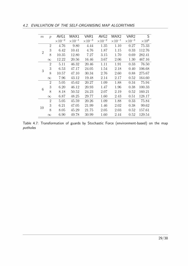
4.7 Transformation of guards by Stochastic Force (environment-based) on the mappotholes . . . . . . . . . . . . . . . . . . . . . . . . . . . . . . . . . . . . . 29

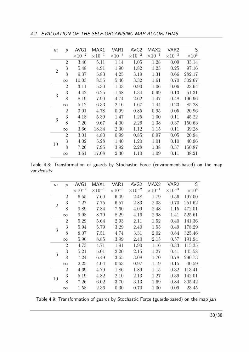
4.8 Transformation of guards by Stochastic Force (environment-based) on the mapvar density . . . . . . . . . . . . . . . . . . . . . . . . . . . . . . . . . . . . 30

4.9 Transformation of guards by Stochastic Force (guards-based) on the map jari . 30

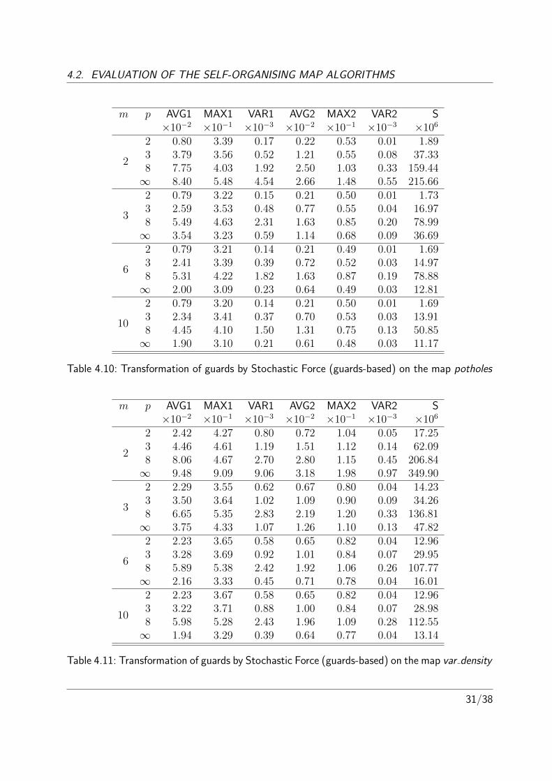
4.10 Transformation of guards by Stochastic Force (guards-based) on the map potholes 31

4.11 Transformation of guards by Stochastic Force (guards-based) on the map var density 31

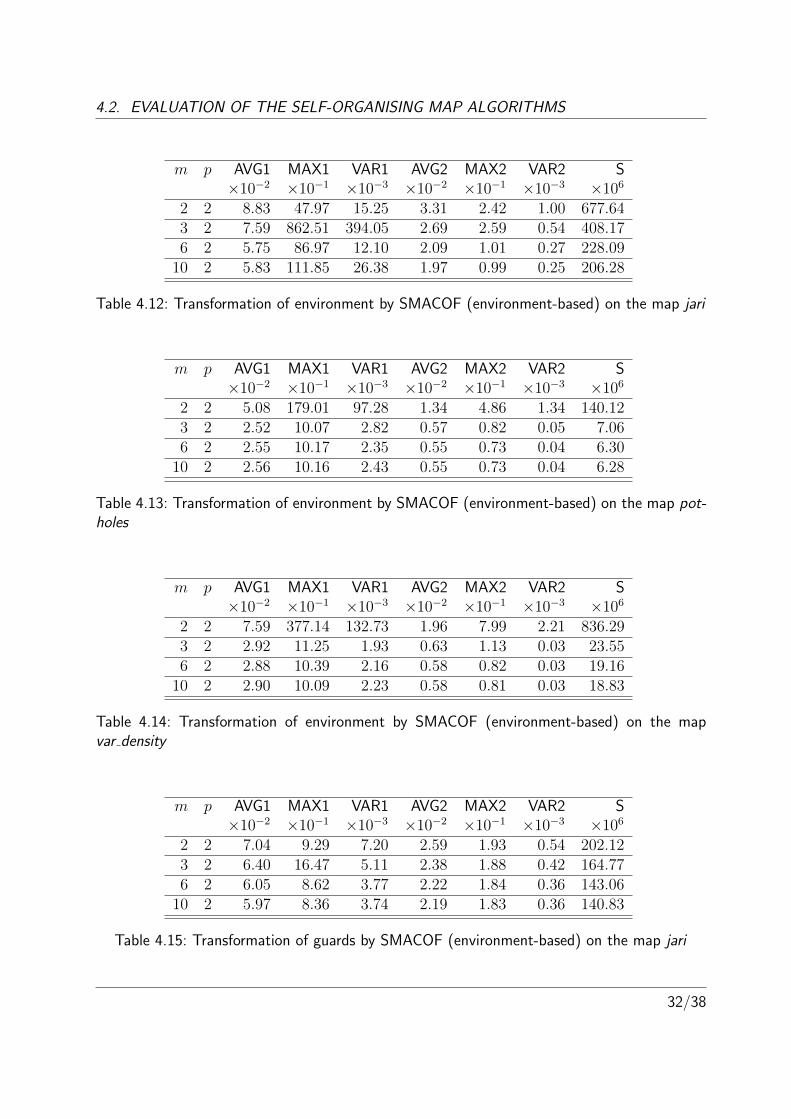
4.12 Transformation of environment by SMACOF (environment-based) on the map jari 32

4.13 Transformation of environment by SMACOF (environment-based) on the mappotholes . . . . . . . . . . . . . . . . . . . . . . . . . . . . . . . . . . . . . 32

4.14 Transformation of environment by SMACOF (environment-based) on the mapvar density . . . . . . . . . . . . . . . . . . . . . . . . . . . . . . . . . . . . 32

4.15 Transformation of guards by SMACOF (environment-based) on the map jari . 32

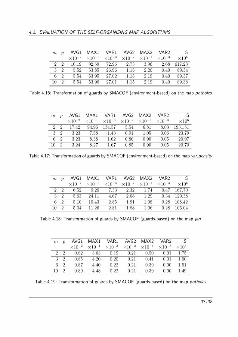
4.16 Transformation of guards by SMACOF (environment-based) on the map potholes 33

4.17 Transformation of guards by SMACOF (environment-based) on the map var density 33

4.18 Transformation of guards by SMACOF (guards-based) on the map jari . . . . 33

iii

LIST OF TABLES

4.19 Transformation of guards by SMACOF (guards-based) on the map potholes . . 33

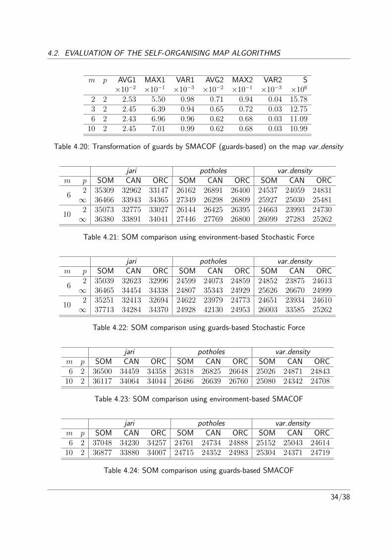
4.20 Transformation of guards by SMACOF (guards-based) on the map var density 34

4.21 SOM comparison using environment-based Stochastic Force . . . . . . . . . . 34

4.22 SOM comparison using guards-based Stochastic Force . . . . . . . . . . . . . 34

4.23 SOM comparison using environment-based SMACOF . . . . . . . . . . . . . . 34

4.24 SOM comparison using guards-based SMACOF . . . . . . . . . . . . . . . . . 34

5.1 CD Content . . . . . . . . . . . . . . . . . . . . . . . . . . . . . . . . . . . 38

iv

LIST OF ALGORITHMS

List of algorithms

1 The proposed algorithm . . . . . . . . . . . . . . . . . . . . . . . . . . . . . . 5

2 SOM training . . . . . . . . . . . . . . . . . . . . . . . . . . . . . . . . . . . 7

3 Basic SOM and CAN . . . . . . . . . . . . . . . . . . . . . . . . . . . . . . . 7

4 ORC-SOM training . . . . . . . . . . . . . . . . . . . . . . . . . . . . . . . . 10

5 Distance matrix computing . . . . . . . . . . . . . . . . . . . . . . . . . . . . 11

6 SMACOF . . . . . . . . . . . . . . . . . . . . . . . . . . . . . . . . . . . . . 12

7 Stochastic Force . . . . . . . . . . . . . . . . . . . . . . . . . . . . . . . . . . 13

8 Guards transformation, environment-based approach . . . . . . . . . . . . . . . 17

9 Guards transformation, guards-based approach . . . . . . . . . . . . . . . . . . 17

10 Stochastic force termination . . . . . . . . . . . . . . . . . . . . . . . . . . . 20

1/38

Chapter 1

Introduction

Travelling salesman problem (TSP) is a classic NP-hard problem. It can be stated as aproblem of finding the shortest closed path between a set of cities (guards). Generally, theTSP is a graph problem (guards are represented by the vertices, and the weights of the edgesrepresent distances between the guards). The metric TSP is a special case of the general TSP.In the metric TSP, the guards have coordinates, and the distances can be computed accordingto the used metric. One of the widely known instance of the metric TSP is the Euclidean TSP,where the Euclidean distance is used. Self-organising maps [1] (SOM) have been used [2][3][4]for solving the Euclidean travelling salesman problem.

Developing fast and reliable algorithms for TSP solving in a polygonal domain is importantfor mobile robot navigation. Many areas populated by humans can be modelled in a polygonaldomain, such as floorplans, parks and streets. It is not necessary to know the optimal toursince the environments are frequently dynamic, so temporary or moving obstacles (such aspeople) would corrupt the implementation of the optimal tour anyway. Hence, fast heuristicsare valuable in such cases.

A method of solving the TSP in a polygonal domain by using self-organising maps is coveredin this thesis. Multidimensional scaling (MDS) algorithms are used here to transform a TSP ina polygonal domain into a metric TSP. Two MDS algorithms and three SOM algorithms werechosen for that purpose.

The thesis is structured as follows: in chapter 2 the used approach and the used algorithmsare described. In chapter 3 the implementation (including the changes of the used algorithms) isdiscussed. The experiments and the discussion of the results are covered in chapter 4. Chapter 5is the conclusion.

2/38

Chapter 2

Algorithm description

The algorithm searches for the Travelling Salesman Problem (TSP) solution in a polygonaldomain. TSP consists of finding the shortest route that visits all objects (guards) from a givenset at least once and returns to the first guard in the list (the input is a set of guards, theoutput is an order list of the guards). Polygonal domain So is an environment that consists ofa two-dimensional map with guards and polygonal boundaries and obstacles.

TSP is an NP-hard problem that can be solved by various approaches. Both heuristic andnon-heuristic methods of solving this problem have been developed. The exact solution of theTSP can be found by evaluating all possible tours (all permutations of the set of guards) withcomputational complexity O(n!), which makes this approach impractical. Other methods thatreduce the time complexity have been developed, such as Held–Karp, which is a more sophis-ticated method of solving the TSP with time complexity O(n22n). There is also a number ofheuristics that produce a solution that is not necessarily optimal. They are important because theoptimal solution is not always required in the real-life problems, where the computation speedis more important. These heuristics include: constructive heuristics (greedy algorithm), itera-tive improvement(k-opt, or Lin-Kernighan heuristics [5]) and randomised improvement(geneticalgorithms [6], ant colony optimisation algorithm [7]).

It has been proposed [2][3][4] to use Self-Organising maps [1] (SOM) for the Euclidean TSPand for the TSP in a polygonal domain [8][9]. SOM is a kind of a neural network. Input of thatnetwork is the coordinates of a guard. For each input that has been fed into the network neuronschange their weights: the winning neuron (the closest) and its neighbours move towards theinput. By feeding the guards that have to be visited into the network repeatedly, the neuronsconverge to a state from which we can find a tour.

The map in Fig. 2.1a is jari, which is a floorplan of a real building. 4 guards are shown asthe red circles. The neurons (blue circles) initially lie on a small ring. As already mentioned, theguards are repeatedly fed into the neural network. After the current input (the guard markedby a yellow dot in Fig. 2.1) has been fed into the SOM, the neurons reorganise as shown inFig. 2.1b: the winning neuron (the neuron marked by a yellow dot in Fig. 2.1) and its neighbours

3/38

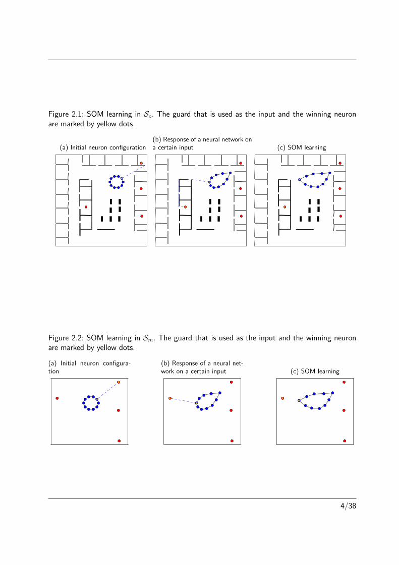
Figure 2.1: SOM learning in So. The guard that is used as the input and the winning neuronare marked by yellow dots.

(a) Initial neuron configuration(b) Response of a neural network ona certain input (c) SOM learning

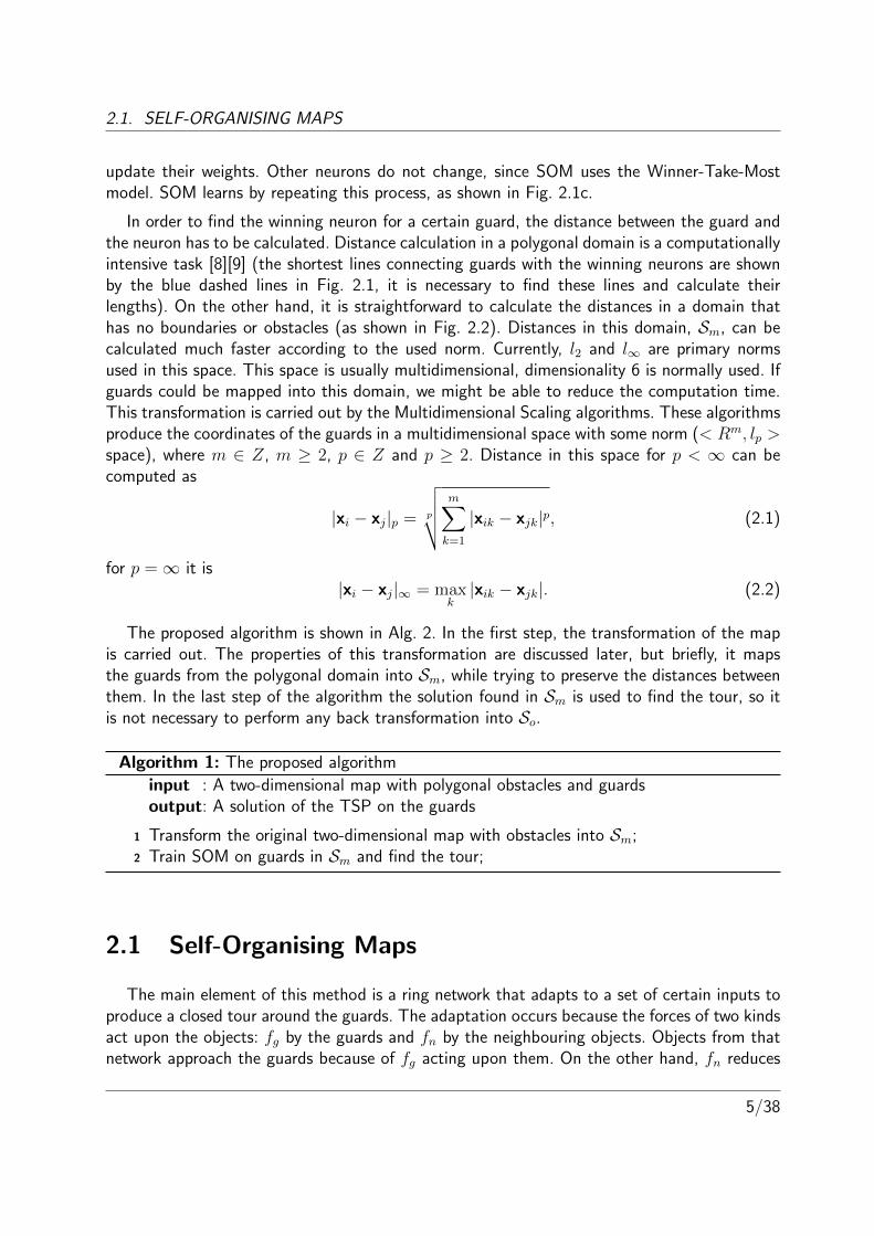
Figure 2.2: SOM learning in Sm. The guard that is used as the input and the winning neuronare marked by yellow dots.

(a) Initial neuron configura-tion

(b) Response of a neural net-work on a certain input (c) SOM learning

4/38

2.1. SELF-ORGANISING MAPS

update their weights. Other neurons do not change, since SOM uses the Winner-Take-Mostmodel. SOM learns by repeating this process, as shown in Fig. 2.1c.

In order to find the winning neuron for a certain guard, the distance between the guard andthe neuron has to be calculated. Distance calculation in a polygonal domain is a computationallyintensive task [8][9] (the shortest lines connecting guards with the winning neurons are shownby the blue dashed lines in Fig. 2.1, it is necessary to find these lines and calculate theirlengths). On the other hand, it is straightforward to calculate the distances in a domain thathas no boundaries or obstacles (as shown in Fig. 2.2). Distances in this domain, Sm, can becalculated much faster according to the used norm. Currently, l2 and l∞ are primary normsused in this space. This space is usually multidimensional, dimensionality 6 is normally used. Ifguards could be mapped into this domain, we might be able to reduce the computation time.This transformation is carried out by the Multidimensional Scaling algorithms. These algorithmsproduce the coordinates of the guards in a multidimensional space with some norm (< Rm, lp >space), where m ∈ Z, m ≥ 2, p ∈ Z and p ≥ 2. Distance in this space for p < ∞ can becomputed as

|xi − xj|p = p

√√√√ m∑k=1

|xik − xjk|p, (2.1)

for p =∞ it is|xi − xj|∞ = max

k|xik − xjk|. (2.2)

The proposed algorithm is shown in Alg. 2. In the first step, the transformation of the mapis carried out. The properties of this transformation are discussed later, but briefly, it mapsthe guards from the polygonal domain into Sm, while trying to preserve the distances betweenthem. In the last step of the algorithm the solution found in Sm is used to find the tour, so itis not necessary to perform any back transformation into So.

Algorithm 1: The proposed algorithm

input : A two-dimensional map with polygonal obstacles and guardsoutput: A solution of the TSP on the guards

1 Transform the original two-dimensional map with obstacles into Sm;2 Train SOM on guards in Sm and find the tour;

2.1 Self-Organising Maps

The main element of this method is a ring network that adapts to a set of certain inputs toproduce a closed tour around the guards. The adaptation occurs because the forces of two kindsact upon the objects: fg by the guards and fn by the neighbouring objects. Objects from thatnetwork approach the guards because of fg acting upon them. On the other hand, fn reduces

5/38


the total length of the connections in the network. fn acts like the forces in an expanded rubberband. Several algorithms are based on that idea: Elastic net [10] and algorithms based on theSelf-Organising Map [1] training.

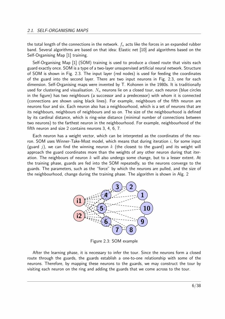
Self-Organising Map [1] (SOM) training is used to produce a closed route that visits eachguard exactly once. SOM is a type of a two-layer unsupervised artificial neural network. Structureof SOM is shown in Fig. 2.3. The input layer (red nodes) is used for feeding the coordinatesof the guard into the second layer. There are two input neurons in Fig. 2.3, one for eachdimension. Self-Organising maps were invented by T. Kohonen in the 1980s. It is traditionallyused for clustering and visualisation. Nn neurons lie on a closed tour, each neuron (blue circlesin the figure) has two neighbours (a successor and a predecessor) with whom it is connected(connections are shown using black lines). For example, neighbours of the fifth neuron areneurons four and six. Each neuron also has a neighbourhood, which is a set of neurons that areits neighbours, neighbours of neighbours and so on. The size of the neighbourhood is definedby its cardinal distance, which is ring-wise distance (minimal number of connections betweentwo neurons) to the farthest neuron in the neighbourhood. For example, neighbourhood of thefifth neuron and size 2 contains neurons 3, 4, 6, 7.

Each neuron has a weight vector, which can be interpreted as the coordinates of the neu-ron. SOM uses Winner-Take-Most model, which means that during iteration i, for some input(guard j), we can find the winning neuron k (the closest to the guard) and its weight willapproach the guard coordinates more than the weights of any other neuron during that iter-ation. The neighbours of neuron k will also undergo some change, but to a lesser extent. Atthe training phase, guards are fed into the SOM repeatedly, so the neurons converge to theguards. The parameters, such as the “force” by which the neurons are pulled, and the size ofthe neighbourhood, change during the training phase. The algorithm is shown in Alg. 2

123

4

5

67 8

9

10i1

i2

Figure 2.3: SOM example

After the learning phase, it is necessary to infer the tour. Since the neurons form a closedroute through the guards, the guards establish a one-to-one relationship with some of theneurons. Therefore, by mapping these neurons to the guards, we may construct the tour byvisiting each neuron on the ring and adding the guards that we come across to the tour.

6/38


Algorithm 2: SOM training

input : Set of guards in an environment without obstaclesoutput: A solution of the TSP on the guards

1 Initialise neurons;2 Pick a guard gi;3 Find the winning neuron nj;4 Update weights of the winner and its neighbours so these neurons approach the

picked guard;5 If the termination condition is satisfied, construct and return tour;6 Update parameters and go to step 2.;

SOM was first proposed for TSP solving in [2]. The implementation proposed in this articleis later referred to as the Basic SOM. Other approaches and implementations include a Co-adaptive neural network [3] and Overall-Regional Competitive Self-Organizing Map [4].

2.1.1 Basic SOM

The algorithm of the basic SOM [2] is shown in Alg. 3

Algorithm 3: Basic SOM and CAN


1 Initialise the neural network;2 Randomise the set of guards;3 Pick the first guard from the set;4 Find the winning neuron;5 Move weights of the winning neuron and its neighbours towards the picked guard;6 Pick the next guard from the set and go to step 4. If there are no guards left,

continue to step 7;7 If the termination condition is satisfied, construct the tour and return it;8 Otherwise, update the parameters and go to step 2.;

In the beginning, the neurons are initialised on a small ring in the centre of the guardsdistribution. A random permutation of the guards is generated at each iteration. The adaptationprocess is based on feeding the guards from the permutation into the SOM. For each of theinputs, the winning neuron is selected.

After the winning neuron has been found, its weights and the weights of its neighbours are

7/38


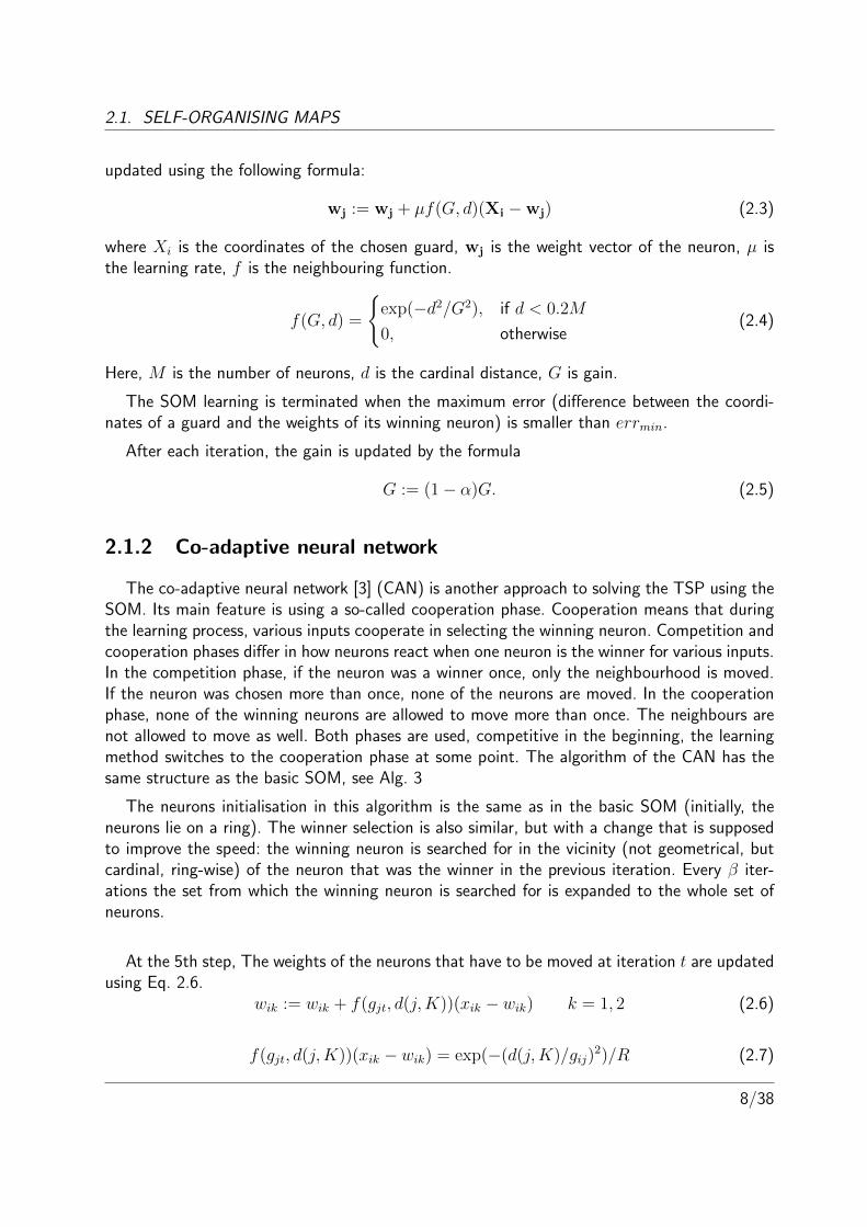
updated using the following formula:

wj := wj + µf(G, d)(Xi −wj) (2.3)

where Xi is the coordinates of the chosen guard, wj is the weight vector of the neuron, µ isthe learning rate, f is the neighbouring function.

f(G, d) =

{exp(−d2/G2), if d < 0.2M

0, otherwise(2.4)

Here, M is the number of neurons, d is the cardinal distance, G is gain.

The SOM learning is terminated when the maximum error (difference between the coordi-nates of a guard and the weights of its winning neuron) is smaller than errmin.

After each iteration, the gain is updated by the formula

G := (1− α)G. (2.5)

2.1.2 Co-adaptive neural network

The co-adaptive neural network [3] (CAN) is another approach to solving the TSP using theSOM. Its main feature is using a so-called cooperation phase. Cooperation means that duringthe learning process, various inputs cooperate in selecting the winning neuron. Competition andcooperation phases differ in how neurons react when one neuron is the winner for various inputs.In the competition phase, if the neuron was a winner once, only the neighbourhood is moved.If the neuron was chosen more than once, none of the neurons are moved. In the cooperationphase, none of the winning neurons are allowed to move more than once. The neighbours arenot allowed to move as well. Both phases are used, competitive in the beginning, the learningmethod switches to the cooperation phase at some point. The algorithm of the CAN has thesame structure as the basic SOM, see Alg. 3

The neurons initialisation in this algorithm is the same as in the basic SOM (initially, theneurons lie on a ring). The winner selection is also similar, but with a change that is supposedto improve the speed: the winning neuron is searched for in the vicinity (not geometrical, butcardinal, ring-wise) of the neuron that was the winner in the previous iteration. Every β iter-ations the set from which the winning neuron is searched for is expanded to the whole set ofneurons.

At the 5th step, The weights of the neurons that have to be moved at iteration t are updatedusing Eq. 2.6.

wik := wik + f(gjt, d(j,K))(xik − wik) k = 1, 2 (2.6)

f(gjt, d(j,K))(xik − wik) = exp(−(d(j,K)/gij)2)/R (2.7)

8/38


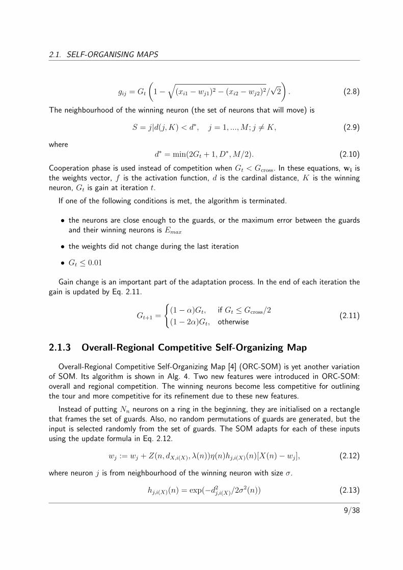
gij = Gt

(1−

√(xi1 − wj1)2 − (xi2 − wj2)2/

√2

). (2.8)

The neighbourhood of the winning neuron (the set of neurons that will move) is

S = j|d(j,K) < d∗, j = 1, ...,M ; j 6= K, (2.9)

whered∗ = min(2Gt + 1, D∗,M/2). (2.10)

Cooperation phase is used instead of competition when Gt < Gcross. In these equations, wi isthe weights vector, f is the activation function, d is the cardinal distance, K is the winningneuron, Gt is gain at iteration t.

If one of the following conditions is met, the algorithm is terminated.

• the neurons are close enough to the guards, or the maximum error between the guardsand their winning neurons is Emax

• the weights did not change during the last iteration

• Gt ≤ 0.01

Gain change is an important part of the adaptation process. In the end of each iteration thegain is updated by Eq. 2.11.

Gt+1 =

{(1− α)Gt, if Gt ≤ Gcross/2

(1− 2α)Gt, otherwise(2.11)

2.1.3 Overall-Regional Competitive Self-Organizing Map

Overall-Regional Competitive Self-Organizing Map [4] (ORC-SOM) is yet another variationof SOM. Its algorithm is shown in Alg. 4. Two new features were introduced in ORC-SOM:overall and regional competition. The winning neurons become less competitive for outliningthe tour and more competitive for its refinement due to these new features.

Instead of putting Nn neurons on a ring in the beginning, they are initialised on a rectanglethat frames the set of guards. Also, no random permutations of guards are generated, but theinput is selected randomly from the set of guards. The SOM adapts for each of these inputsusing the update formula in Eq. 2.12.

wj := wj + Z(n, dX,i(X), λ(n))η(n)hj,i(X)(n)[X(n)− wj], (2.12)

where neuron j is from neighbourhood of the winning neuron with size σ.

hj,i(X)(n) = exp(−d2j,i(X)/2σ2(n)) (2.13)

9/38

2.2. MULTIDIMENSIONAL SCALING

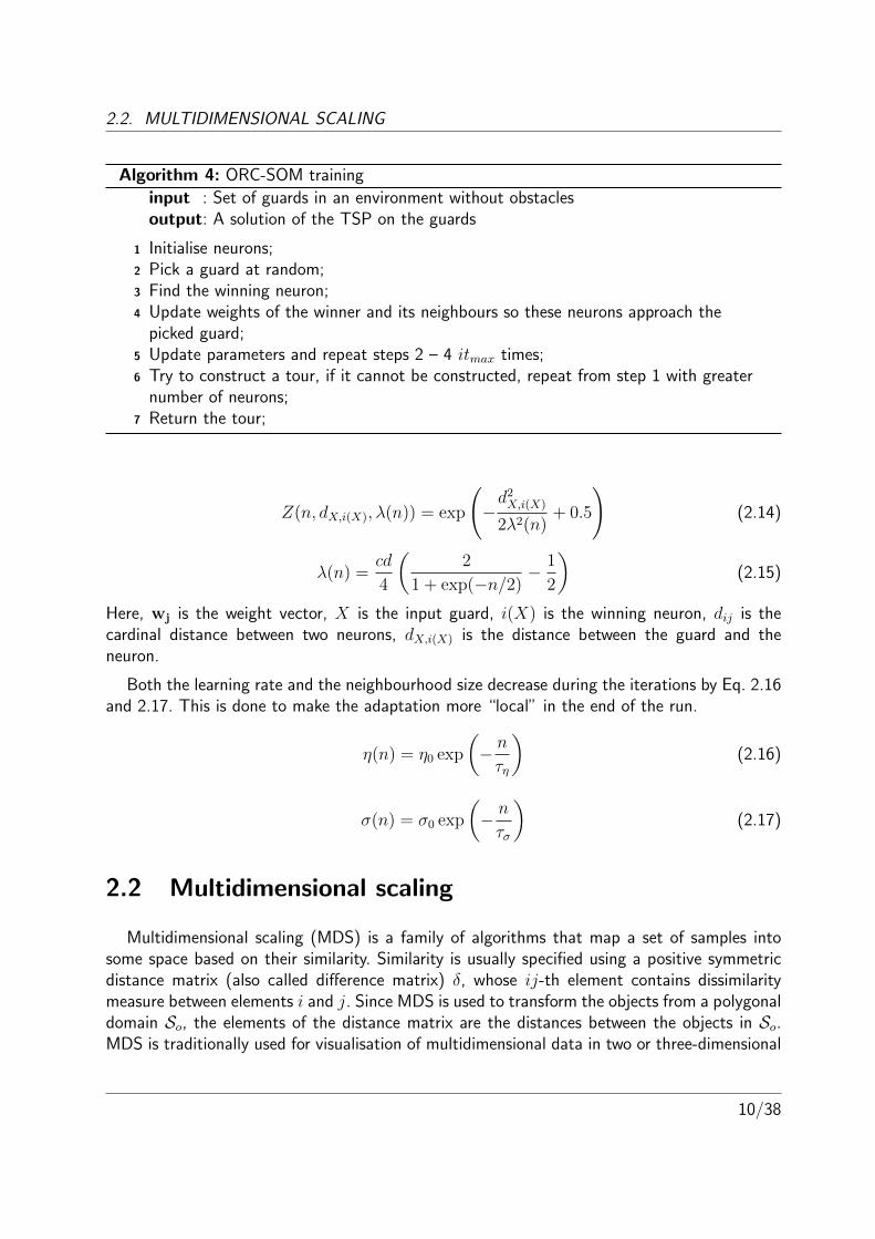
Algorithm 4: ORC-SOM training


1 Initialise neurons;2 Pick a guard at random;3 Find the winning neuron;4 Update weights of the winner and its neighbours so these neurons approach the

picked guard;5 Update parameters and repeat steps 2 – 4 itmax times;6 Try to construct a tour, if it cannot be constructed, repeat from step 1 with greater

number of neurons;7 Return the tour;

Z(n, dX,i(X), λ(n)) = exp

(−d2X,i(X)

2λ2(n)+ 0.5

)(2.14)

λ(n) =cd

4

(2

1 + exp(−n/2)− 1

2

)(2.15)

Here, wj is the weight vector, X is the input guard, i(X) is the winning neuron, dij is thecardinal distance between two neurons, dX,i(X) is the distance between the guard and theneuron.

Both the learning rate and the neighbourhood size decrease during the iterations by Eq. 2.16and 2.17. This is done to make the adaptation more “local” in the end of the run.

η(n) = η0 exp

(− nτη

)(2.16)

σ(n) = σ0 exp

(− nτσ

)(2.17)

2.2 Multidimensional scaling

Multidimensional scaling (MDS) is a family of algorithms that map a set of samples intosome space based on their similarity. Similarity is usually specified using a positive symmetricdistance matrix (also called difference matrix) δ, whose ij-th element contains dissimilaritymeasure between elements i and j. Since MDS is used to transform the objects from a polygonaldomain So, the elements of the distance matrix are the distances between the objects in So.MDS is traditionally used for visualisation of multidimensional data in two or three-dimensional

10/38


space (or, mapping multidimensional data into low-dimensional space). In the produced output,similar objects are mapped close to each other forming clusters.

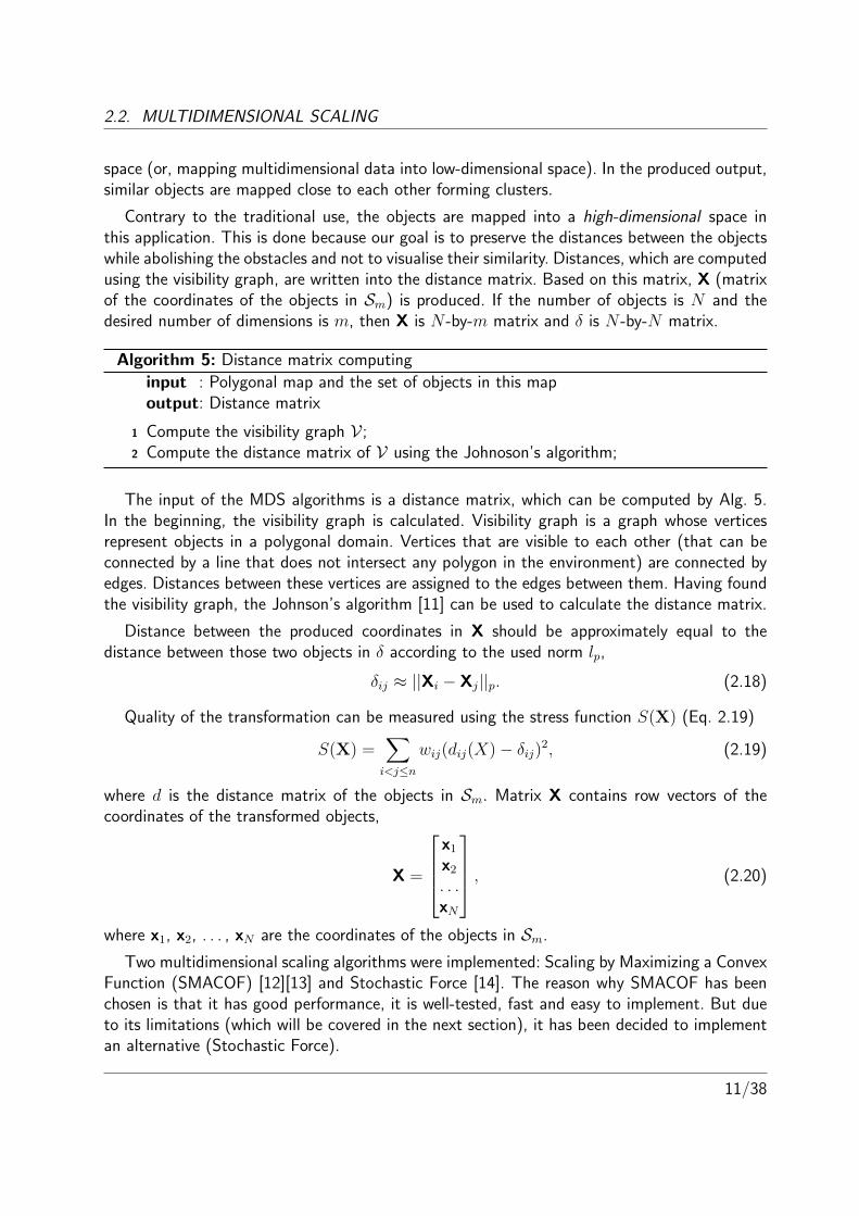
Contrary to the traditional use, the objects are mapped into a high-dimensional space inthis application. This is done because our goal is to preserve the distances between the objectswhile abolishing the obstacles and not to visualise their similarity. Distances, which are computedusing the visibility graph, are written into the distance matrix. Based on this matrix, X (matrixof the coordinates of the objects in Sm) is produced. If the number of objects is N and thedesired number of dimensions is m, then X is N -by-m matrix and δ is N -by-N matrix.

Algorithm 5: Distance matrix computing

input : Polygonal map and the set of objects in this mapoutput: Distance matrix

1 Compute the visibility graph V ;2 Compute the distance matrix of V using the Johnoson’s algorithm;

The input of the MDS algorithms is a distance matrix, which can be computed by Alg. 5.In the beginning, the visibility graph is calculated. Visibility graph is a graph whose verticesrepresent objects in a polygonal domain. Vertices that are visible to each other (that can beconnected by a line that does not intersect any polygon in the environment) are connected byedges. Distances between these vertices are assigned to the edges between them. Having foundthe visibility graph, the Johnson’s algorithm [11] can be used to calculate the distance matrix.

Distance between the produced coordinates in X should be approximately equal to thedistance between those two objects in δ according to the used norm lp,

δij ≈ ||Xi − Xj||p. (2.18)

Quality of the transformation can be measured using the stress function S(X) (Eq. 2.19)

S(X) =∑i<j≤n

wij(dij(X)− δij)2, (2.19)

where d is the distance matrix of the objects in Sm. Matrix X contains row vectors of thecoordinates of the transformed objects,

X =

x1

x2

. . .xN

, (2.20)

where x1, x2, . . . , xN are the coordinates of the objects in Sm.

Two multidimensional scaling algorithms were implemented: Scaling by Maximizing a ConvexFunction (SMACOF) [12][13] and Stochastic Force [14]. The reason why SMACOF has beenchosen is that it has good performance, it is well-tested, fast and easy to implement. But dueto its limitations (which will be covered in the next section), it has been decided to implementan alternative (Stochastic Force).

11/38


2.2.1 Scaling by Maximizing a Convex Function

SMACOF is based on stress majorisation. It means that instead of minimising S(X), we canminimise a function τ(X,Z) that is always greater than or equal to S(X). It can be shownthat the following function satisfies that condition:

τ = η2δ + tr(XTV X)− 2tr(XTB(Z)Z). (2.21)

We can find the minimum of τ by setting its derivative to zero:

∇Xτ(X,Z) = 0 + 2V X − 2B(Z)Z = 0, (2.22)

from which we can find X asX = V +B(Z)Z, (2.23)

or, if the weights are equal to one,

X = N−1B(Z)Z (2.24)

SMACOF is an iterative algorithm, and Eq. 2.24 is used as the update formula at eachiteration. SMACOF is shown in Alg. 6

Algorithm 6: SMACOF

input : Distance matrix δoutput: Coordinates of the objects in Sm, X

1 Set the iteration number i = 0, Z = X0 (random initial configuration);2 Compute the stress using Eq. 2.19;3 Increment i;4 Compute the next solution Xi by Eq. 2.24;5 If the stress change is small, Si−1 − Si < ε, return Xi;6 Go to step 3;

Note that in the 5th step, stress difference is computed, and not its absolute value. Thisis done because stress is always decreasing (in distinction to Stochastic Force, another MDSalgorithm). SMACOF was derived using the Cauchy-Schwarz inequality [12], which is truefor inner product spaces. Spaces with lp norm, where p 6= 2 are not inner product spaces,therefore they cannot be used by SMACOF. It can be shown that some basic shapes cannot betransformed into desired space without introducing an error. An example of such a shape is asquare obstacle, which is covered in Chapter 3.

2.2.2 Stochastic force

Theoretically, SMACOF allows only l2 norm, so it is impossible to experiment with othernorms to find out whether they would yield better results. Because of that, Stochastic Force

12/38


was implemented. The idea behind this algorithm is that we can simulate spring-like forcesbetween the transformed objects in order to carry out that transformation. The force betweena pair of objects pushes them apart if they are closer to each other than in So, or towards eachother if they are farther than in So. The word stochastic comes from the method of computingthe forces: they are not calculated for all pairs at each iteration, but rather for two sets: a set ofrandomly selected objects Vi and a set of pairs of neighbouring objects Si. This approach hastwo advantages: it adds jitters to prevent from converging to local optima, while showing goodperformance for neighbouring objects. Vi is reinitialised at every iteration, while Si is randomat first, but it converges to a set of neighbouring objects in time. It is done by the followingrule: while populating Vi, if some candidate to Vi is closer than the farthest object from Si, addit to Si instead of Vi. The sizes of these sets are set to Vmax, Smax. The objects movement issimulated using the Euler method.

Euler method is a method for numerical solving of differential equations. Given the systemddty(t) = f(t,y(t), the solution is approximated by the equation

yk+1 = yn + hf(tn, yn) (2.25)

here, h is the integration step. Since the spring-like forces are simulated, f and y and be definedas

yk =

[vkxk

](2.26)

f(t, yk) =

[Fkvk

](2.27)

where Fk is the force acting on the object. Therefore, Eq. 2.25 can be rewritten as[vk+1

xk+1

]=

[vkxk

]+ h

[Fkvk

], (2.28)

which is used as the update formula at each iteration. Other, more complicated simulationalgorithms exist, but it is not necessary to implement them because accurate simulation is notwhat we are after. For the same reason, h does not have to be too small to yield good results,which is covered later. The procedure is shown in Alg. 7

Algorithm 7: Stochastic Force

input : Distance matrix δoutput: Coordinates of the objects in Sm

1 (Re)initialise V , S of all objects;2 Compute forces acting upon all objects;3 Make a simulation step;4 If the termination condition is satisfied, return the coordinates of the objects;5 If it is not satisfied, go to step 1;

13/38


At the first step, random objects are added to V (also, S, if it is the first iteration) with aconstraint: no repeating objects are allowed in the sets. Reorganise the objects from both setsby adding the closest ones to S and the rest to V .

At the second step, the sum of all forces that act upon object i by objects from Vi and Siis calculated. The magnitude of the force acting upon object i by object j is proportional togij − δij (the difference between the distance in Sm and in So). This force is directed towardsthe object j. For the purpose of stabilisation, the magnitude of the forces is limited to flim, soafter the sum has been computed, it is necessary to clip some forces.

Next, the simulation step is made. First, compute the velocities using Eq. 2.29.

vi = µ(vi + fih) (2.29)

Here, µ is the friction constant, whose purpose is stabilisation of the system. After the velocitieshave been updated, compute the new coordinates using the expression

xi = xi + vih (2.30)

The advantage of this algorithm over SMACOF is that it allows using norms other than theEuclidean.

14/38

Chapter 3

Implementation

Algorithms described in the previous sections were implemented. The program was writtenin C++ programming language with external C++ libraries: VTK, Boost, Eigen, VisiLibity.Triangle library written in pure C was also used.

VTK (Visualization Toolkit, http://www.vtk.org/) is an open-source, cross-platform C++library (interfaces for Tcl/Tk, Java and Python are also available) developed by Kitware. VTKis used for visualisation, image processing and computer graphics. Although VTK is very fea-ture rich, it was used mainly for visualisation of the algorithms. The recommended version ofthis library is 6.0+, but it is mostly compatible with version 5.8. The implementation can becompiled without VTK, since it is used only for visualisation.

Boost (http://www.boost.org/) is a set of cross-platform open-source C++ libraries.The range of its applications is wide. It is used for graph algorithms, linear algebra operations,math algorithms, multithreading and other purposes. It contains over 80 libraries. In this im-plementation, it is used for reading of the command-line switches (in Boost.Program options)and for its graph algorithms (Boost.Graph).

Eigen C++ library (http://eigen.tuxfamily.org/) is used for matrix calculations. It isan open-source template library used for algorithms related to linear algebra. It is widely usedin scientific projects and by corporations for machine learning, robotics, numerical computationand other applications.

VisiLibity (http://www.visilibity.org/) enables us to compute the visibility graph ofa polygonal map. It is a free open-source C++ library for visibility algorithms. It is used forplanning, navigation, manufacturing and other areas. It is aimed to enable programmers toperform simple visibility calculations in the polygonal domain.

Triangle (https://www.cs.cmu.edu/~quake/triangle.html) is used for calculation ofthe Delaunay triangulation of a polygonal map. It is an open-source C library developed atCarnegie Mellon University. It can be used both as a library and an executable for creatingthe Delaunay triangulations, the constrained Delaunay triangualations, Voronoi diagrams and

15/38


triangular meshes. It supports various parameters of the available algorithms (e.g. forcing edgesfor Delaunay triangulation, setting the smallest allowed angle of triangles and others).

CMake (http://www.cmake.org/) is used as a build manager, but it is possible to buildthe project without it.

The input (environment and guards) format is based on the map (.txt) format used in theIntelligent and Mobile Robotics Group (http://imr.ciirc.cvut.cz/planning/maps.xml).The rules are more strict though. The map file contains vertices that describe the map. The fileis divided into sections. A section represents a polygon (first section contains the descriptionof the map borders and the following sections describe borders). Each section starts with aline [borders]. Each of the following lines in the section contain two real numbers dividedby a space (the coordinates of the vertex). The sections finish in an empty line. No repeatingvertices or obstacles are allowed.

The guards file starts with a line [guards] that follows by Nn lines that contain the coor-dinates of the guards. Each of these lines contains two real numbers (as in the map file).

Both files have two empty lines in the bottom. The guards must lie within the map boundaries.The polygons from the map file cannot overlay. The vertices of the map boundaries and theobstacles must be listed counterclockwise.

3.1 Self-Organising maps

The original algorithms were designed for the two-dimensional Euclidean space < R2, l2 >,but other spaces were also used in this implementation, so it was necessary to make somechanges to the algorithms. In the beginning of the network learning, the neurons have to beinitialised. Depending on the used algorithm, they can be initialised either on a small ring, oron a frame around the guards. This initialisation is unambiguous in a two-dimensional space,but in Sm different initial weights are possible. The easiest one is to ignore higher dimensions(set the corresponding weights to zero) and initialise the neurons as though the neurons arein the two-dimensional space. Because of the increased number of dimensions, the structure ofSOM changes as well: instead of 2 input neurons in Fig. 2.3, it is necessary to use m neuronsin the input layer, since SOM is used in Sm with m dimensions.

3.2 Multidimensional scaling

Input of the MDS algorithms is a distance matrix δ, whose elements contain distancesbetween the transformed objects (δij = d(i, j)). In order to produce that matrix, the followinglibraries and algorithms were used:

• VisiLibity, a library for 2D visibility algorithms. Algorithm for visibility graph computationfrom this library has time complexity O(n3),

16/38


• Johnoson’s algorithm for distance matrix computing from Boost library.

There are two ways of transforming the guards from So into Sm: the first method isenvironment-based (indirect method), which means that the coordinates of the guards in Smare not computed directly, but the estimate of their location is based on the existing transfor-mation of the environment, as shown in Alg. 8. In the alternative approach (Alg. 9), the guardsare transformed directly (guards-based method).

Algorithm 8: Guards transformation, environment-based approach

input : A polygonal map, a set of guardsoutput: Mapping of the guards into Sm

1 Compute the distance matrix of the vertices of the polygons of the map by Alg.5;2 Transform the distance matrix into Sm using MDS;3 Create Delaunay triangulation of So map, forcing edges of the obstacles to be edges

of triangles;4 Approximate the coordinates of the guards in Sm;

Algorithm 9: Guards transformation, guards-based approach

input : A polygonal map, a set of guardsoutput: Mapping of the guards into Sm

1 Compute the difference matrix of the guards by Alg.5;2 Transform the difference matrix into Sm using one of the MDS methods;

Both methods have advantages and disadvantages. The direct method allows us to transformthe map into Sm once, and use it for various sets of guards, saving some time. It is faster toapproximate the coordinates of the guards in Sm than to actually transform them using MDSfor every new set of guards on the same map. On the other hand, the second approach mightproduce better results in some cases, since the coordinates are not approximated but computeddirectly. It is worth mentioning that the results will not necessarily be improved by using thesecond method. For example, if the used map is jari from Fig. 2.1, and there is maximum oneguard per room, the error introduced by approximation of the coordinates of the guards is smallrelatively to the distances between the guards, therefore, the first approach should be used.

If the environment-based approach is used, the coordinates of the guards have to be approx-imated. First, the triangulation of the map is created and for each guard i a triangle t in whichit lies is found. [

xiyi

]=

[aAx + bBx + cCxaAy + bBy + cCy

], (3.1)

a+ b+ c = 1, (3.2)

17/38


where (xi, yi)T is the coordinates vector of the guard i, (Ax, Ay)

T , (Bx, By)T , (Cx, Cy)

T are thecoordinates of the vertices of the triangle t and a, b, c are the weights that have to be found.Eqs. 3.1 and 3.2 can be rewritten asxiyi

1

=

Ax Bx CxAy By Cy1 1 1

abc

, (3.3)

and the weights can be computed asabc

=

Ax Bx CxAy By Cy1 1 1

−1 xiyi1

. (3.4)

Coordinates in Sm can be computed as

xim = aAm + bBm + cCm (3.5)

3.2.1 SMACOF

It was found that the proposed termination criterion is not robust. The authors suggested tohalt the algorithm when the stress difference is small, Si−1 − Si < ε. Since the value of stresscan vary in different environments, setting ε to some predefined value may be inadequate. Itis also difficult to guess the appropriate value of ε for a chosen map. Because of that, thetermination method was changed to Si−1−Si

Si< ε.

Limitations

As mentioned earlier, some obstacles cannot be transformed into Sm with l2 norm. Anexample of such an object is a square obstacle. Distance matrix of the vertices of a square withsides of unity length is

D =

0 1 2 11 0 1 22 1 0 11 2 1 0

(3.6)

The best result can be achieved by setting the number of dimensions to three. Setting it toa greater number will not improve the transformation since four vertices will always lie in athree-dimensional subspace. In order to carry out that transformation, we can start by puttingthe vertices on a unit square:

X =

x1

x2

x3

x4

=

0 0 00 1 01 1 01 0 0

(3.7)

18/38


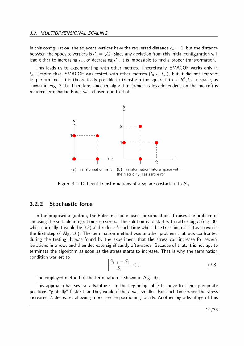
In this configuration, the adjacent vertices have the requested distance da = 1, but the distancebetween the opposite vertices is do =

√2. Since any deviation from this initial configuration will

lead either to increasing da, or decreasing do, it is impossible to find a proper transformation.

This leads us to experimenting with other metrics. Theoretically, SMACOF works only inl2. Despite that, SMACOF was tested with other metrics (l3, l8, l∞), but it did not improveits performance. It is theoretically possible to transform the square into < R2, l∞ > space, asshown in Fig. 3.1b. Therefore, another algorithm (which is less dependent on the metric) isrequired. Stochastic Force was chosen due to that.

y

x

1

1

(a) Transformation in l2

y

x

2

1

1

2

(b) Transformation into a space withthe metric l∞ has zero error

Figure 3.1: Different transformations of a square obstacle into Sm

3.2.2 Stochastic force

In the proposed algorithm, the Euler method is used for simulation. It raises the problem ofchoosing the suitable integration step size h. The solution is to start with rather big h (e.g. 30,while normally it would be 0.3) and reduce h each time when the stress increases (as shown inthe first step of Alg. 10). The termination method was another problem that was confrontedduring the testing. It was found by the experiment that the stress can increase for severaliterations in a row, and then decrease significantly afterwards. Because of that, it is not apt toterminate the algorithm as soon as the stress starts to increase. That is why the terminationcondition was set to ∣∣∣∣Si−1 − SiSi

∣∣∣∣ < ε (3.8)

The employed method of the termination is shown in Alg. 10.

This approach has several advantages. In the beginning, objects move to their appropriatepositions “globally” faster than they would if the h was smaller. But each time when the stressincreases, h decreases allowing more precise positioning locally. Another big advantage of this

19/38


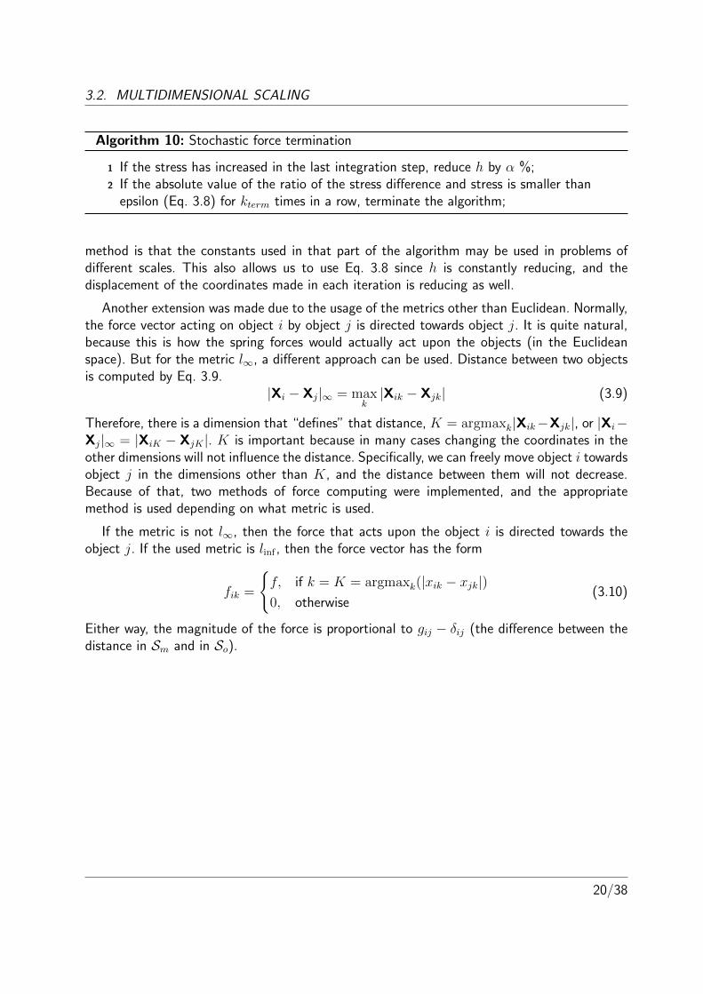
Algorithm 10: Stochastic force termination

1 If the stress has increased in the last integration step, reduce h by α %;2 If the absolute value of the ratio of the stress difference and stress is smaller than

epsilon (Eq. 3.8) for kterm times in a row, terminate the algorithm;

method is that the constants used in that part of the algorithm may be used in problems ofdifferent scales. This also allows us to use Eq. 3.8 since h is constantly reducing, and thedisplacement of the coordinates made in each iteration is reducing as well.

Another extension was made due to the usage of the metrics other than Euclidean. Normally,the force vector acting on object i by object j is directed towards object j. It is quite natural,because this is how the spring forces would actually act upon the objects (in the Euclideanspace). But for the metric l∞, a different approach can be used. Distance between two objectsis computed by Eq. 3.9.

|Xi − Xj|∞ = maxk|Xik − Xjk| (3.9)

Therefore, there is a dimension that “defines” that distance, K = argmaxk|Xik−Xjk|, or |Xi−Xj|∞ = |XiK − XjK |. K is important because in many cases changing the coordinates in theother dimensions will not influence the distance. Specifically, we can freely move object i towardsobject j in the dimensions other than K, and the distance between them will not decrease.Because of that, two methods of force computing were implemented, and the appropriatemethod is used depending on what metric is used.

If the metric is not l∞, then the force that acts upon the object i is directed towards theobject j. If the used metric is linf , then the force vector has the form

fik =

{f, if k = K = argmaxk(|xik − xjk|)0, otherwise

(3.10)

Either way, the magnitude of the force is proportional to gij − δij (the difference between thedistance in Sm and in So).

20/38

Chapter 4

Experiments

The algorithms described in the previous chapters were tested. Since a great number ofexperiments was required, a lot of processing power was necessary. This was made possiblethanks to the National Grid Infrastructure MetaCentrum, which provided a cluster for parallelcomputation of the experiments.

4.1 Evaluation of the multidimensional scaling algorithms

First, it is necessary to analyse the MDS algorithms. As already mentioned, two MDS al-gorithms were implemented: Stochastic Force and SMACOF. Different space dimensions andnorms were used: Stochastic Force was tested with dimensions R2, R3, R6, R10 and norms l2,l3, l8, l∞. SMACOF was tested with dimensions R2, R3, R6, R10 and l2 norm.

(a) jari (b) potholes (c) var density

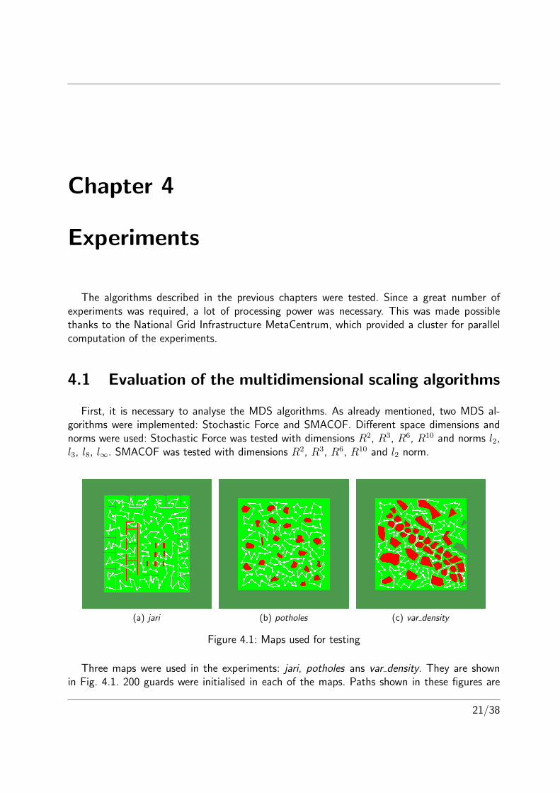
Figure 4.1: Maps used for testing

Three maps were used in the experiments: jari, potholes ans var density. They are shownin Fig. 4.1. 200 guards were initialised in each of the maps. Paths shown in these figures are

21/38

4.1. EVALUATION OF THE MULTIDIMENSIONAL SCALING ALGORITHMS

examples of the solutions found using the developed procedure. They were found by ORCSOMand guards-based Stochastic Force.

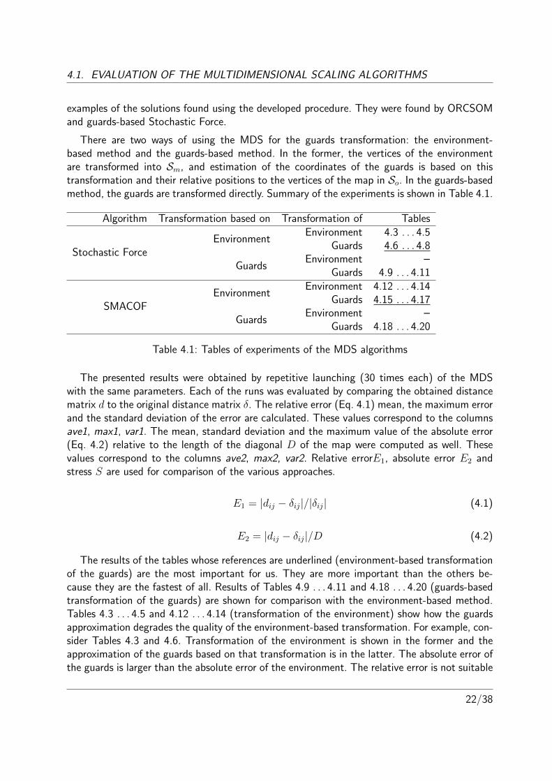
There are two ways of using the MDS for the guards transformation: the environment-based method and the guards-based method. In the former, the vertices of the environmentare transformed into Sm, and estimation of the coordinates of the guards is based on thistransformation and their relative positions to the vertices of the map in So. In the guards-basedmethod, the guards are transformed directly. Summary of the experiments is shown in Table 4.1.

Algorithm Transformation based on Transformation of Tables

Stochastic ForceEnvironment

Environment 4.3 . . . 4.5Guards 4.6 . . . 4.8

GuardsEnvironment –

Guards 4.9 . . . 4.11

SMACOFEnvironment

Environment 4.12 . . . 4.14Guards 4.15 . . . 4.17

GuardsEnvironment –

Guards 4.18 . . . 4.20

Table 4.1: Tables of experiments of the MDS algorithms

The presented results were obtained by repetitive launching (30 times each) of the MDSwith the same parameters. Each of the runs was evaluated by comparing the obtained distancematrix d to the original distance matrix δ. The relative error (Eq. 4.1) mean, the maximum errorand the standard deviation of the error are calculated. These values correspond to the columnsave1, max1, var1. The mean, standard deviation and the maximum value of the absolute error(Eq. 4.2) relative to the length of the diagonal D of the map were computed as well. Thesevalues correspond to the columns ave2, max2, var2. Relative errorE1, absolute error E2 andstress S are used for comparison of the various approaches.

E1 = |dij − δij|/|δij| (4.1)

E2 = |dij − δij|/D (4.2)

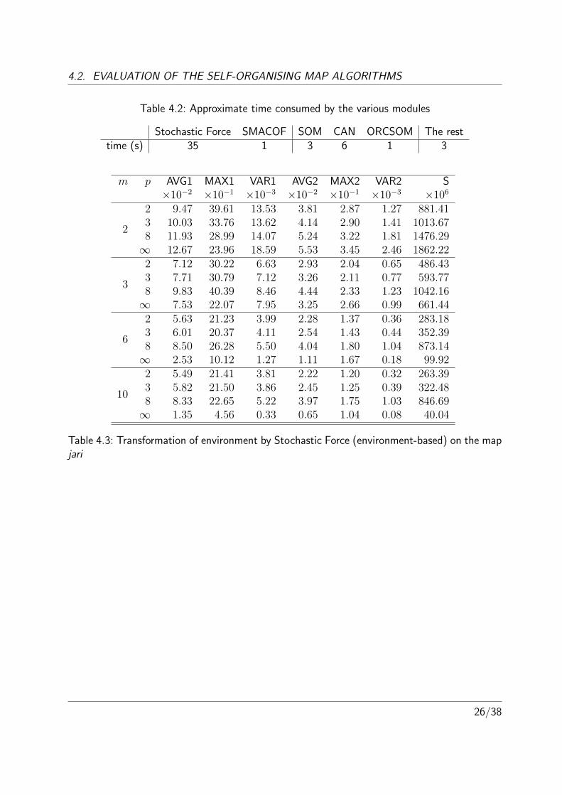
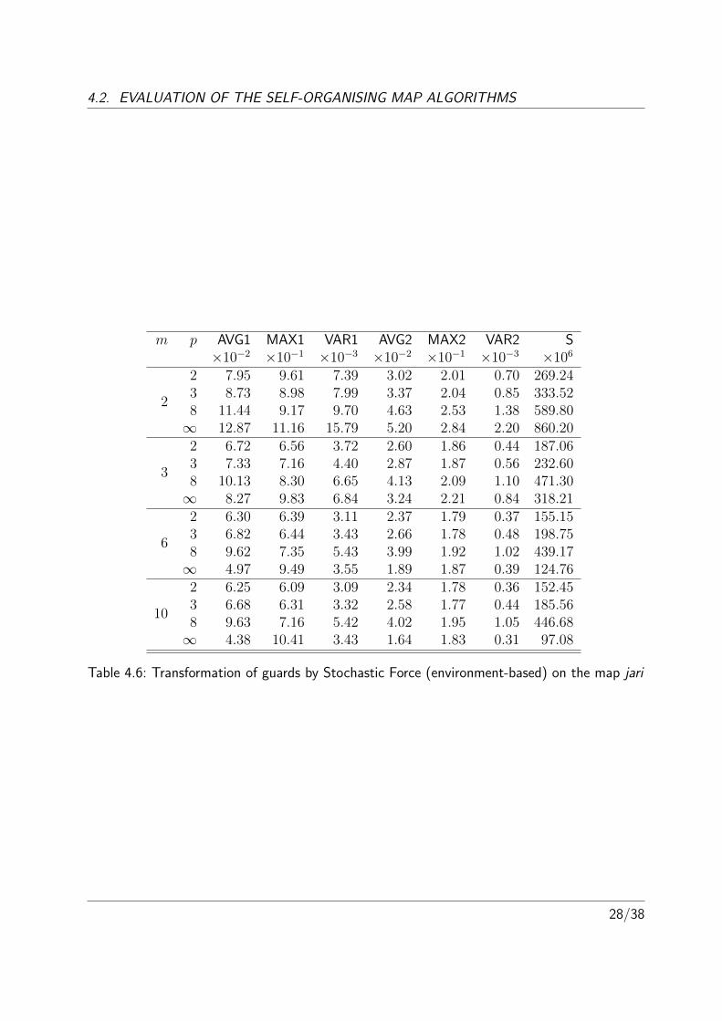
The results of the tables whose references are underlined (environment-based transformationof the guards) are the most important for us. They are more important than the others be-cause they are the fastest of all. Results of Tables 4.9 . . . 4.11 and 4.18 . . . 4.20 (guards-basedtransformation of the guards) are shown for comparison with the environment-based method.Tables 4.3 . . . 4.5 and 4.12 . . . 4.14 (transformation of the environment) show how the guardsapproximation degrades the quality of the environment-based transformation. For example, con-sider Tables 4.3 and 4.6. Transformation of the environment is shown in the former and theapproximation of the guards based on that transformation is in the latter. The absolute error ofthe guards is larger than the absolute error of the environment. The relative error is not suitable

22/38

4.1. EVALUATION OF THE MULTIDIMENSIONAL SCALING ALGORITHMS

for that comparison because the objects that are close to each other are prone to having largerrelative error, and the vertices of the map can be often quite close.

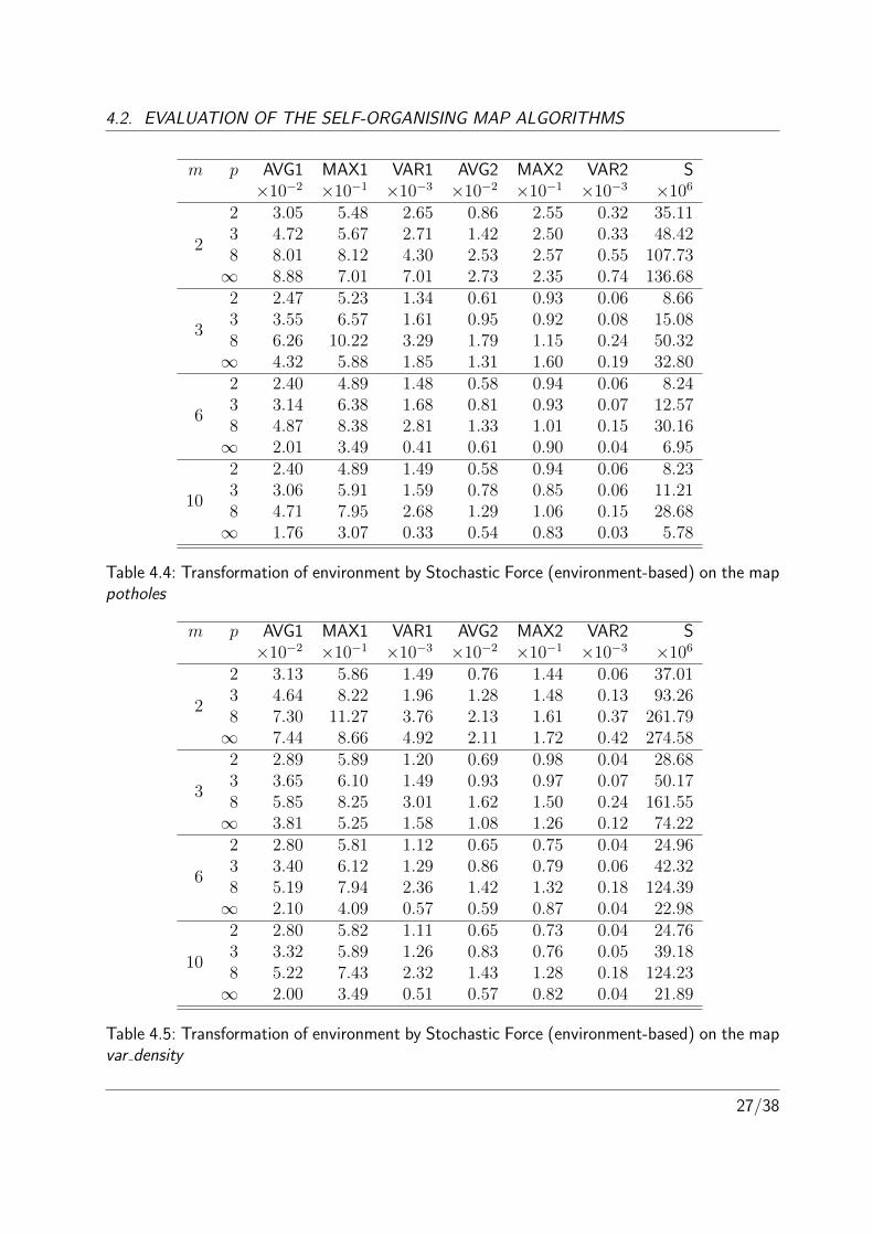
From the obtained values we can make some observations and evaluate the quality of thetransformations. First of all, the stress decreases when the larger number of dimensions is used.The question is when this effect becomes small. Usually, the quality of the guards transformation(measured by the error) does not improve significantly by using the number of dimensions largerthan 6. In one case using R10 reduced the stress almost by half comparing to R6), so it wasdecided to keep experimenting with the number of dimensions m = 10. Different maps requiredifferent m. The greater number of dimensions is necessary for the jari -type maps that havecomplex non-convex obstacles (for example, maps with rooms). If the obstacles are mostlyconvex, the necessity of using a greater number of dimensions decreases. For example, usingR6 instead of R3 reduces stress by 5% in potholes, and by 42% in jari (Tables 4.4, 4.3)

It is difficult to choose the most suitable norm, because it varies in different maps. Using l∞seems to produce better transformations in jari (Tables 4.3, 4.6, 4.9), but it is worse in potholes(Tables 4.4, 4.7, 4.10). The performance of l3 and l8 was always worse than the performanceof the other tested norms. Quality improvement of l∞ comparing to l3 and l8 is caused by usingmodified forces in the Stochastic Force algorithm for l∞. It is also important to notice that ifthe environment-based transformation is used, some quality loss is inevitable. Since the usedmethod of the guards estimation was developed for l2, the quality loss is larger when l∞ is used.

The most significant difference between the direct and the indirect method can be observedin the potholes map, where the stress is about 10 times greater in the environment-basedapproach, which is observed in both Stochastic Force and SMACOF. (Tables 4.7, 4.10 and 4.7,4.10) While in the other maps the difference is not so noticeable, it is difficult to guess howthis error induced by guards approximation will affect the tour length of the obtained solutionwithout actually testing both methods.

Similarly to Stochastic Force, the recommended choice of the number of dimensions forSMACOF is around 6. An interesting observation is that SMACOF performs much worse thenStochastic Force in R2. This is caused by inability of SMACOF to break out of the local optima.

Mostly, the quality of the transformation by SMACOF and Stochastic Force is similar, withthe exception of the jari map, where l∞ is more suitable, and therefore, cannot be used inSMACOF. In the used implementation, SMACOF is much faster than Stochastic Force. UnlikeSMACOF, Stochastic Force has many parameters that can be tuned (Vmax, Smax, α and others),so its quality can be improved for various maps.

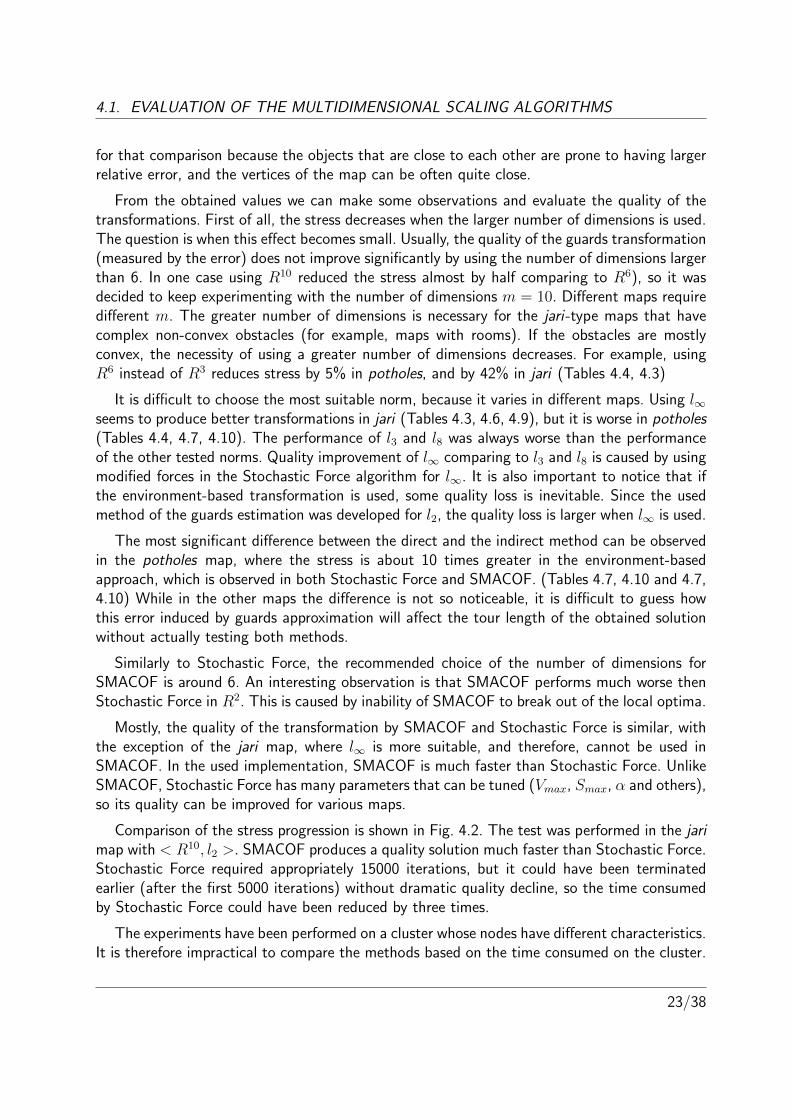
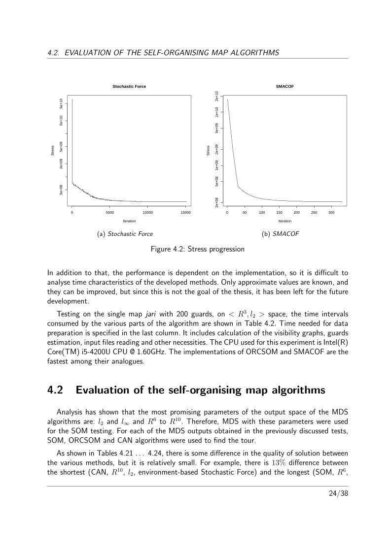
Comparison of the stress progression is shown in Fig. 4.2. The test was performed in the jarimap with < R10, l2 >. SMACOF produces a quality solution much faster than Stochastic Force.Stochastic Force required appropriately 15000 iterations, but it could have been terminatedearlier (after the first 5000 iterations) without dramatic quality decline, so the time consumedby Stochastic Force could have been reduced by three times.

The experiments have been performed on a cluster whose nodes have different characteristics.It is therefore impractical to compare the methods based on the time consumed on the cluster.

23/38

4.2. EVALUATION OF THE SELF-ORGANISING MAP ALGORITHMS

0 5000 10000 15000

5e+

082e

+09

5e+

092e

+10

5e+

10

Stochastic Force

Iteration

Str

ess

(a) Stochastic Force

0 50 100 150 200 250 3002e

+08

5e+

081e

+09

2e+

095e

+09

1e+

102e

+10

SMACOF

Iteration

Str

ess

(b) SMACOF

Figure 4.2: Stress progression

In addition to that, the performance is dependent on the implementation, so it is difficult toanalyse time characteristics of the developed methods. Only approximate values are known, andthey can be improved, but since this is not the goal of the thesis, it has been left for the futuredevelopment.

Testing on the single map jari with 200 guards, on < R3, l2 > space, the time intervalsconsumed by the various parts of the algorithm are shown in Table 4.2. Time needed for datapreparation is specified in the last column. It includes calculation of the visibility graphs, guardsestimation, input files reading and other necessities. The CPU used for this experiment is Intel(R)Core(TM) i5-4200U CPU @ 1.60GHz. The implementations of ORCSOM and SMACOF are thefastest among their analogues.

4.2 Evaluation of the self-organising map algorithms

Analysis has shown that the most promising parameters of the output space of the MDSalgorithms are: l2 and l∞ and R6 to R10. Therefore, MDS with these parameters were usedfor the SOM testing. For each of the MDS outputs obtained in the previously discussed tests,SOM, ORCSOM and CAN algorithms were used to find the tour.

As shown in Tables 4.21 . . . 4.24, there is some difference in the quality of solution betweenthe various methods, but it is relatively small. For example, there is 13% difference betweenthe shortest (CAN, R10, l2, environment-based Stochastic Force) and the longest (SOM, R6,

24/38


l2, guards-based SMACOF) tour length for jari. For Stochastic Force, l∞ does not seem todecrease the tour length, otherwise, the results produced when using this norm are generallyworse than the results of the traditional Euclidean norm. Moreover, two unusually lengthy tourswere found using the guards-based Stochastic Force in R10, l∞ in potholes and var density. Thiserror appears because the SOM algorithms were developed for the two-dimensional Euclideanspace, so maybe some changes are necessary to improve their behaviour in other spaces, but inthe current implementation l2 is the better choice.

SOM, CAN and ORCSOM produce results of the similar quality in potholes, var density, butin jari the results produced by the basic SOM are worse. Therefore, CAN and ORCSOM seemto be more robust. R10 is slightly better than R6 in most instances, but the difference is notsignificant.

Guards-based approach was expected to improve the results, but it is not the case. Evenwhen it does produce the shorter tour, the time that was consumed by the MDS does not payoff in the quality improvement. And finally, the choice of the MDS algorithm does not influencethe quality, therefore, the less time-consuming (SMACOF) should be chosen.

25/38


Table 4.2: Approximate time consumed by the various modules

Stochastic Force SMACOF SOM CAN ORCSOM The resttime (s) 35 1 3 6 1 3

m p AVG1 MAX1 VAR1 AVG2 MAX2 VAR2 S×10−2 ×10−1 ×10−3 ×10−2 ×10−1 ×10−3 ×106

2

2 9.47 39.61 13.53 3.81 2.87 1.27 881.413 10.03 33.76 13.62 4.14 2.90 1.41 1013.678 11.93 28.99 14.07 5.24 3.22 1.81 1476.29∞ 12.67 23.96 18.59 5.53 3.45 2.46 1862.22

3

2 7.12 30.22 6.63 2.93 2.04 0.65 486.433 7.71 30.79 7.12 3.26 2.11 0.77 593.778 9.83 40.39 8.46 4.44 2.33 1.23 1042.16∞ 7.53 22.07 7.95 3.25 2.66 0.99 661.44

6

2 5.63 21.23 3.99 2.28 1.37 0.36 283.183 6.01 20.37 4.11 2.54 1.43 0.44 352.398 8.50 26.28 5.50 4.04 1.80 1.04 873.14∞ 2.53 10.12 1.27 1.11 1.67 0.18 99.92

10

2 5.49 21.41 3.81 2.22 1.20 0.32 263.393 5.82 21.50 3.86 2.45 1.25 0.39 322.488 8.33 22.65 5.22 3.97 1.75 1.03 846.69∞ 1.35 4.56 0.33 0.65 1.04 0.08 40.04

Table 4.3: Transformation of environment by Stochastic Force (environment-based) on the mapjari

26/38



2

2 3.05 5.48 2.65 0.86 2.55 0.32 35.113 4.72 5.67 2.71 1.42 2.50 0.33 48.428 8.01 8.12 4.30 2.53 2.57 0.55 107.73∞ 8.88 7.01 7.01 2.73 2.35 0.74 136.68

3

2 2.47 5.23 1.34 0.61 0.93 0.06 8.663 3.55 6.57 1.61 0.95 0.92 0.08 15.088 6.26 10.22 3.29 1.79 1.15 0.24 50.32∞ 4.32 5.88 1.85 1.31 1.60 0.19 32.80

6

2 2.40 4.89 1.48 0.58 0.94 0.06 8.243 3.14 6.38 1.68 0.81 0.93 0.07 12.578 4.87 8.38 2.81 1.33 1.01 0.15 30.16∞ 2.01 3.49 0.41 0.61 0.90 0.04 6.95

10

2 2.40 4.89 1.49 0.58 0.94 0.06 8.233 3.06 5.91 1.59 0.78 0.85 0.06 11.218 4.71 7.95 2.68 1.29 1.06 0.15 28.68∞ 1.76 3.07 0.33 0.54 0.83 0.03 5.78

Table 4.4: Transformation of environment by Stochastic Force (environment-based) on the mappotholes


2

2 3.13 5.86 1.49 0.76 1.44 0.06 37.013 4.64 8.22 1.96 1.28 1.48 0.13 93.268 7.30 11.27 3.76 2.13 1.61 0.37 261.79∞ 7.44 8.66 4.92 2.11 1.72 0.42 274.58

3

2 2.89 5.89 1.20 0.69 0.98 0.04 28.683 3.65 6.10 1.49 0.93 0.97 0.07 50.178 5.85 8.25 3.01 1.62 1.50 0.24 161.55∞ 3.81 5.25 1.58 1.08 1.26 0.12 74.22

6

2 2.80 5.81 1.12 0.65 0.75 0.04 24.963 3.40 6.12 1.29 0.86 0.79 0.06 42.328 5.19 7.94 2.36 1.42 1.32 0.18 124.39∞ 2.10 4.09 0.57 0.59 0.87 0.04 22.98

10

2 2.80 5.82 1.11 0.65 0.73 0.04 24.763 3.32 5.89 1.26 0.83 0.76 0.05 39.188 5.22 7.43 2.32 1.43 1.28 0.18 124.23∞ 2.00 3.49 0.51 0.57 0.82 0.04 21.89

Table 4.5: Transformation of environment by Stochastic Force (environment-based) on the mapvar density

27/38



2

2 7.95 9.61 7.39 3.02 2.01 0.70 269.243 8.73 8.98 7.99 3.37 2.04 0.85 333.528 11.44 9.17 9.70 4.63 2.53 1.38 589.80∞ 12.87 11.16 15.79 5.20 2.84 2.20 860.20

3

2 6.72 6.56 3.72 2.60 1.86 0.44 187.063 7.33 7.16 4.40 2.87 1.87 0.56 232.608 10.13 8.30 6.65 4.13 2.09 1.10 471.30∞ 8.27 9.83 6.84 3.24 2.21 0.84 318.21

6

2 6.30 6.39 3.11 2.37 1.79 0.37 155.153 6.82 6.44 3.43 2.66 1.78 0.48 198.758 9.62 7.35 5.43 3.99 1.92 1.02 439.17∞ 4.97 9.49 3.55 1.89 1.87 0.39 124.76

10

2 6.25 6.09 3.09 2.34 1.78 0.36 152.453 6.68 6.31 3.32 2.58 1.77 0.44 185.568 9.63 7.16 5.42 4.02 1.95 1.05 446.68∞ 4.38 10.41 3.43 1.64 1.83 0.31 97.08

Table 4.6: Transformation of guards by Stochastic Force (environment-based) on the map jari

28/38



2

2 4.76 9.80 4.44 1.35 1.10 0.27 75.333 6.42 10.41 4.76 1.87 1.15 0.33 112.768 10.35 12.80 7.27 3.15 1.70 0.69 282.41∞ 12.22 20.56 16.46 3.67 2.06 1.30 467.16

3

2 5.11 46.32 20.46 1.11 1.91 0.33 76.503 6.53 47.17 24.05 1.54 2.18 0.40 106.688 10.57 47.10 30.34 2.76 2.60 0.88 275.67∞ 7.96 43.12 19.48 2.14 2.17 0.52 164.60

6

2 5.05 45.62 20.27 1.09 1.88 0.34 75.943 6.20 46.12 20.93 1.47 1.96 0.38 100.338 8.18 50.52 24.23 2.07 2.19 0.52 160.21∞ 6.87 48.25 29.77 1.60 2.43 0.51 128.17

10

2 5.05 45.59 20.26 1.09 1.88 0.33 75.843 6.21 47.05 21.99 1.46 2.02 0.38 99.628 8.05 45.29 21.75 2.05 2.03 0.52 157.61∞ 6.90 49.78 30.99 1.60 2.44 0.52 129.54

Table 4.7: Transformation of guards by Stochastic Force (environment-based) on the mappotholes

29/38



2

2 3.40 5.11 1.14 1.05 1.28 0.09 33.143 5.48 4.91 1.90 1.82 1.23 0.25 97.168 9.37 5.83 4.25 3.19 1.31 0.66 282.17∞ 10.03 8.55 5.46 3.32 1.61 0.70 302.67

3

2 3.11 5.30 1.03 0.90 1.06 0.06 23.643 4.42 6.25 1.68 1.34 0.99 0.13 51.318 8.19 7.90 4.74 2.62 1.47 0.48 196.96∞ 5.12 6.33 2.16 1.67 1.44 0.23 85.28

6

2 3.01 4.78 0.99 0.85 0.95 0.05 20.963 4.18 5.39 1.47 1.25 1.00 0.11 45.228 7.20 9.67 4.00 2.26 1.38 0.37 150.63∞ 3.66 18.34 2.30 1.12 1.15 0.11 39.28

10

2 3.01 4.80 0.99 0.85 0.97 0.05 20.943 4.02 5.28 1.40 1.20 1.01 0.10 40.968 7.26 7.95 3.92 2.28 1.38 0.37 150.87∞ 3.61 17.08 2.30 1.10 1.09 0.11 38.21

Table 4.8: Transformation of guards by Stochastic Force (environment-based) on the mapvar density


2

2 6.55 7.60 6.09 2.48 1.79 0.56 197.003 7.27 7.75 6.57 2.83 2.03 0.70 251.628 9.89 7.84 7.60 4.09 2.48 1.15 472.01∞ 9.98 8.79 8.29 4.16 2.98 1.41 525.61

3

2 5.29 5.64 2.93 2.11 1.52 0.40 141.363 5.94 5.79 3.29 2.40 1.55 0.49 178.298 8.07 7.51 4.74 3.31 2.02 0.84 325.46∞ 5.90 8.85 3.99 2.40 2.15 0.57 191.94

6

2 4.73 4.71 1.91 1.90 1.16 0.33 115.353 5.21 5.01 2.20 2.15 1.27 0.41 145.588 7.24 6.49 3.65 3.08 1.70 0.78 290.73∞ 2.25 4.04 0.63 0.97 1.19 0.15 40.59

10

2 4.69 4.79 1.86 1.89 1.15 0.32 113.413 5.19 4.82 2.10 2.13 1.27 0.39 142.018 7.26 6.02 3.70 3.13 1.69 0.84 305.42∞ 1.58 2.36 0.30 0.70 1.00 0.09 23.45

Table 4.9: Transformation of guards by Stochastic Force (guards-based) on the map jari

30/38



2

2 0.80 3.39 0.17 0.22 0.53 0.01 1.893 3.79 3.56 0.52 1.21 0.55 0.08 37.338 7.75 4.03 1.92 2.50 1.03 0.33 159.44∞ 8.40 5.48 4.54 2.66 1.48 0.55 215.66

3

2 0.79 3.22 0.15 0.21 0.50 0.01 1.733 2.59 3.53 0.48 0.77 0.55 0.04 16.978 5.49 4.63 2.31 1.63 0.85 0.20 78.99∞ 3.54 3.23 0.59 1.14 0.68 0.09 36.69

6

2 0.79 3.21 0.14 0.21 0.49 0.01 1.693 2.41 3.39 0.39 0.72 0.52 0.03 14.978 5.31 4.22 1.82 1.63 0.87 0.19 78.88∞ 2.00 3.09 0.23 0.64 0.49 0.03 12.81

10

2 0.79 3.20 0.14 0.21 0.50 0.01 1.693 2.34 3.41 0.37 0.70 0.53 0.03 13.918 4.45 4.10 1.50 1.31 0.75 0.13 50.85∞ 1.90 3.10 0.21 0.61 0.48 0.03 11.17

Table 4.10: Transformation of guards by Stochastic Force (guards-based) on the map potholes


2

2 2.42 4.27 0.80 0.72 1.04 0.05 17.253 4.46 4.61 1.19 1.51 1.12 0.14 62.098 8.06 4.67 2.70 2.80 1.15 0.45 206.84∞ 9.48 9.09 9.06 3.18 1.98 0.97 349.90

3

2 2.29 3.55 0.62 0.67 0.80 0.04 14.233 3.50 3.64 1.02 1.09 0.90 0.09 34.268 6.65 5.35 2.83 2.19 1.20 0.33 136.81∞ 3.75 4.33 1.07 1.26 1.10 0.13 47.82

6

2 2.23 3.65 0.58 0.65 0.82 0.04 12.963 3.28 3.69 0.92 1.01 0.84 0.07 29.958 5.89 5.38 2.42 1.92 1.06 0.26 107.77∞ 2.16 3.33 0.45 0.71 0.78 0.04 16.01

10

2 2.23 3.67 0.58 0.65 0.82 0.04 12.963 3.22 3.71 0.88 1.00 0.84 0.07 28.988 5.98 5.28 2.43 1.96 1.09 0.28 112.55∞ 1.94 3.29 0.39 0.64 0.77 0.04 13.14

Table 4.11: Transformation of guards by Stochastic Force (guards-based) on the map var density

31/38



2 2 8.83 47.97 15.25 3.31 2.42 1.00 677.643 2 7.59 862.51 394.05 2.69 2.59 0.54 408.176 2 5.75 86.97 12.10 2.09 1.01 0.27 228.0910 2 5.83 111.85 26.38 1.97 0.99 0.25 206.28

Table 4.12: Transformation of environment by SMACOF (environment-based) on the map jari


2 2 5.08 179.01 97.28 1.34 4.86 1.34 140.123 2 2.52 10.07 2.82 0.57 0.82 0.05 7.066 2 2.55 10.17 2.35 0.55 0.73 0.04 6.3010 2 2.56 10.16 2.43 0.55 0.73 0.04 6.28

Table 4.13: Transformation of environment by SMACOF (environment-based) on the map pot-holes


2 2 7.59 377.14 132.73 1.96 7.99 2.21 836.293 2 2.92 11.25 1.93 0.63 1.13 0.03 23.556 2 2.88 10.39 2.16 0.58 0.82 0.03 19.1610 2 2.90 10.09 2.23 0.58 0.81 0.03 18.83

Table 4.14: Transformation of environment by SMACOF (environment-based) on the mapvar density


2 2 7.04 9.29 7.20 2.59 1.93 0.54 202.123 2 6.40 16.47 5.11 2.38 1.88 0.42 164.776 2 6.05 8.62 3.77 2.22 1.84 0.36 143.0610 2 5.97 8.36 3.74 2.19 1.83 0.36 140.83

Table 4.15: Transformation of guards by SMACOF (environment-based) on the map jari

32/38



2 2 10.19 92.59 72.96 2.73 3.96 2.68 617.233 2 5.52 53.85 26.96 1.15 2.20 0.40 89.346 2 5.54 53.95 27.02 1.15 2.19 0.40 89.3710 2 5.54 53.90 27.01 1.15 2.19 0.40 89.38

Table 4.16: Transformation of guards by SMACOF (environment-based) on the map potholes


2 2 17.42 94.96 134.57 5.54 6.81 8.03 1931.513 2 3.23 7.58 1.43 0.91 1.05 0.06 23.796 2 3.23 8.38 1.62 0.86 0.90 0.05 20.9710 2 3.24 8.27 1.67 0.85 0.90 0.05 20.70

Table 4.17: Transformation of guards by SMACOF (environment-based) on the map var density


2 2 6.52 9.20 7.33 2.32 1.74 0.47 167.703 2 5.63 24.11 4.67 2.08 1.29 0.34 129.386 2 5.10 10.43 2.85 1.91 1.08 0.28 108.4210 2 5.04 11.26 2.81 1.88 1.06 0.28 106.04

Table 4.18: Transformation of guards by SMACOF (guards-based) on the map jari


2 2 0.82 3.63 0.19 0.21 0.50 0.01 1.753 2 0.85 4.20 0.20 0.21 0.41 0.01 1.606 2 0.87 4.40 0.22 0.21 0.39 0.00 1.5110 2 0.89 4.48 0.22 0.21 0.39 0.00 1.49

Table 4.19: Transformation of guards by SMACOF (guards-based) on the map potholes

33/38



2 2 2.53 5.50 0.98 0.71 0.94 0.04 15.783 2 2.45 6.39 0.94 0.65 0.72 0.03 12.756 2 2.43 6.96 0.96 0.62 0.68 0.03 11.0910 2 2.45 7.01 0.99 0.62 0.68 0.03 10.99

Table 4.20: Transformation of guards by SMACOF (guards-based) on the map var density

jari potholes var densitym p SOM CAN ORC SOM CAN ORC SOM CAN ORC

62 35309 32962 33147 26162 26891 26400 24537 24059 24831∞ 36466 33943 34365 27349 26298 26809 25927 25030 25481

102 35073 32775 33027 26144 26425 26395 24663 23993 24730∞ 36380 33891 34041 27446 27769 26800 26099 27283 25262

Table 4.21: SOM comparison using environment-based Stochastic Force

jari potholes var densitym p SOM CAN ORC SOM CAN ORC SOM CAN ORC

62 35039 32623 32996 24599 24073 24859 24852 23875 24613∞ 36465 34454 34338 24807 35343 24929 25626 26670 24999

102 35251 32413 32694 24622 23979 24773 24651 23934 24610∞ 37713 34284 34370 24928 42130 24953 26003 33585 25262

Table 4.22: SOM comparison using guards-based Stochastic Force

jari potholes var densitym p SOM CAN ORC SOM CAN ORC SOM CAN ORC6 2 36500 34459 34358 26318 26825 26648 25026 24871 2484310 2 36117 34064 34044 26486 26639 26760 25080 24342 24708

Table 4.23: SOM comparison using environment-based SMACOF

jari potholes var densitym p SOM CAN ORC SOM CAN ORC SOM CAN ORC6 2 37048 34230 34257 24761 24734 24888 25152 25043 2461410 2 36877 33880 34007 24715 24352 24983 25304 24371 24719

Table 4.24: SOM comparison using guards-based SMACOF

34/38

Chapter 5

Conclusion

A method for solving the travelling salesman problem in a polygonal domain was presentedin the thesis. It is based on a transformation of the polygonal domain into a metric space usingthe multidimensional scaling algorithms.

The MDS methods were used for application of the SOM algorithms for the Euclidean TSPin a polygonal domain. Different MDS methods with various parameters were implemented andtested. The SOM algorithms used in this experiment were designed for the two-dimensionalEuclidean spaces < R2, l2 >, but they were applied in more general < Rm, lp >.

The experiments have shown that the developed approach works. However, since the algo-rithms were used in an nontraditional way, it is safe to conclude that their performance is notoptimal, and it can be improved.

Various parameters (number of dimensions, norm, guards-based and environment-based ap-proach) were tested, but it did not become clear what parameters are the most suitable, althoughsome of the tested parameters (l3, l8) were excluded. Since a number of variations have shownpromising results, several algorithm modifications can be developed based on this approach.

Currently, guards transformation leads to a poor local performance (for example, small loopsemerge), therefore developing a better method of the local guards positioning (especially for l∞norm) may improve the produced results. Both direct and indirect methods have this problem.Development of a new SOM algorithm that is more apt for l∞ and various numbers of dimensionscould also greatly influence the quality of the solution. It is also necessary to optimise thetermination of Stochastic Force to improve its speed. Other multidimensional scaling algorithmsmay be tested, especially Glimmer [15], which uses stochastic force as a module and has a GPUimplementation, allowing parallel computations.

35/38

BIBLIOGRAPHY

Bibliography

[1] Teuvo Kohonen. Self-organized formation of topologically correct feature maps. BiologicalCybernetics, 43(1):59–69, 1982.

[2] Samerkae Somhom, Abdolhamid Modares, and Takao Enkawa. A self-organising modelfor the travelling salesman problem. Journal of the Operational Research Society, pages919–928, 1997.

[3] EM Cochrane and JE Beasley. The co-adaptive neural network approach to the euclideantravelling salesman problem. Neural Networks, 16(10):1499–1525, 2003.

[4] Junying Zhang, Xuerong Feng, Bin Zhou, and Dechang Ren. An overall-regional com-petitive self-organizing map neural network for the euclidean traveling salesman problem.Neurocomputing, 89:1–11, 2012.

[5] Keld Helsgaun. An effective implementation of the lin–kernighan traveling salesman heuris-tic. European Journal of Operational Research, 126(1):106–130, 2000.

[6] Licheng Jiao and Lei Wang. A novel genetic algorithm based on immunity. Systems, Manand Cybernetics, Part A: Systems and Humans, IEEE Transactions on, 30(5):552–561,2000.

[7] Marco Dorigo and Luca Maria Gambardella. Ant colony system: a cooperative learningapproach to the traveling salesman problem. Evolutionary Computation, IEEE Transactionson, 1(1):53–66, 1997.

[8] Jan Faigl, Miroslav Kulich, Vojtech Vonasek, and Libor Preucil. An application of theself-organizing map in the non-euclidean traveling salesman problem. Neurocomputing,74(5):671–679, 2011.

[9] Jan Faigl. On the performance of self-organizing maps for the non-euclidean travelingsalesman problem in the polygonal domain. Information Sciences, 181(19):4214–4229,2011.

[10] Richard Durbin and David Willshaw. An analogue approach to the travelling salesmanproblem using an elastic net method. Nature, (326):689–91, 1987.

36/38

BIBLIOGRAPHY

[11] Donald B Johnson. Efficient algorithms for shortest paths in sparse networks. Journal ofthe ACM (JACM), 24(1):1–13, 1977.

[12] Ingwer Borg and Patrick JF Groenen. Modern multidimensional scaling: Theory and ap-plications. Springer Science & Business Media, 2005.

[13] Asi Elad and Ron Kimmel. On bending invariant signatures for surfaces. Pattern Analysisand Machine Intelligence, IEEE Transactions on, 25(10):1285–1295, 2003.

[14] Matthew Chalmers. A linear iteration time layout algorithm for visualising high-dimensionaldata. In Visualization’96. Proceedings., pages 127–131. IEEE, 1996.

[15] Stephen Ingram, Tamara Munzner, and Marc Olano. Glimmer: Multilevel mds on the gpu.Visualization and Computer Graphics, IEEE Transactions on, 15(2):249–261, 2009.

37/38

Appendix

CD Content

In table 5.1 are listed names of all root directories on CD

Directory name Descriptionmaps Maps used for testingsompd Source code of the implementation

Table 5.1: CD Content

Self-Organizing Structures for the Travelling Salesman ...

Documents

Transcript of Self-Organizing Structures for the Travelling Salesman ...