Concrete Pavement Surface Characteristics Program Pavement Surface Characteristics Program ......
79
Concrete Pavement Surface Characteristics Program Site Evaluation Report Site 211-1 (Pre- and Post- Grinding/Grooving, Pre-Traffic) Site 211-2 (Post-Traffic, 1 week) Two-Lift Concrete Paving Demonstration Project Eastbound Interstate 70 Solomon, Kansas Tested 8-20 October 2008 (211-1) and 1 November 2008 (211-2) Reported 6 November 2008 (Report Version 3.0) 2711 South Loop Drive, Ste. 4700 Ames, Iowa, 50010 515.294.5798 www.SurfaceCharacteristics.com
Transcript of Concrete Pavement Surface Characteristics Program Pavement Surface Characteristics Program ......

Concrete PavementSurface Characteristics Program
Site Evaluation Report
Site 211-1(Pre- and Post- Grinding/Grooving, Pre-Traffic)
Site 211-2(Post-Traffic, 1 week)
Two-Lift Concrete PavingDemonstration Project
Eastbound Interstate 70Solomon, Kansas
Tested 8-20 October 2008 (211-1) and1 November 2008 (211-2)
Reported 6 November 2008(Report Version 3.0)
2711 South Loop Drive, Ste. 4700Ames, Iowa, 50010
515.294.5798www.SurfaceCharacteristics.com
CPSCP Site Evaluation Report
1
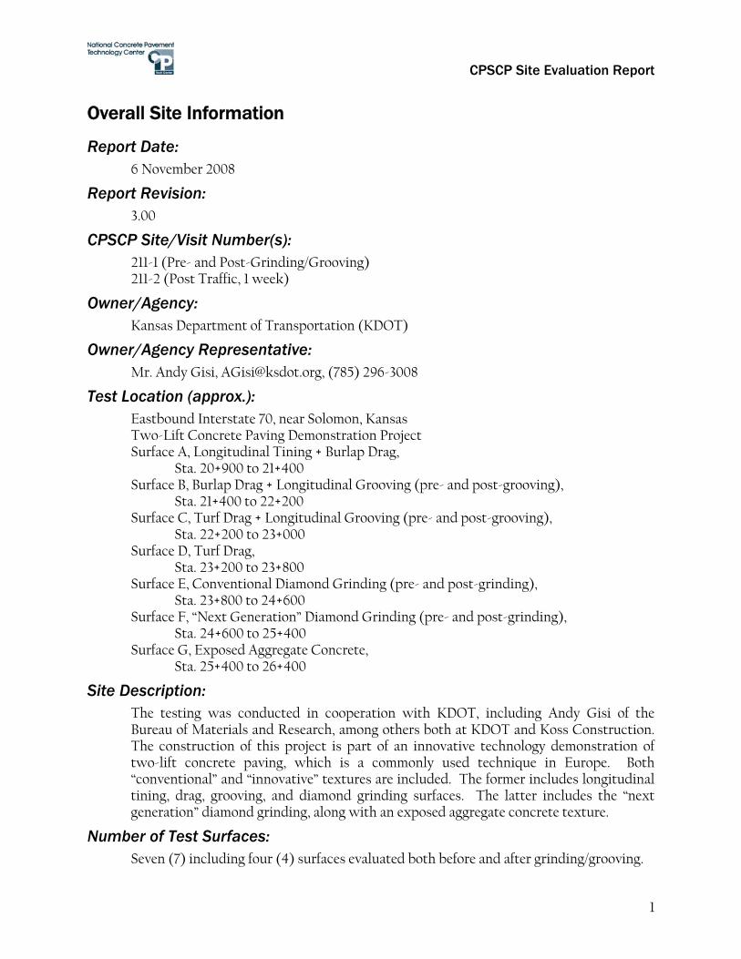
Overall Site Information
Report Date: 6 November 2008
Report Revision: 3.00
CPSCP Site/Visit Number(s): 211-1 (Pre- and Post-Grinding/Grooving) 211-2 (Post Traffic, 1 week)
Owner/Agency: Kansas Department of Transportation (KDOT)
Owner/Agency Representative: Mr. Andy Gisi, [email protected], (785) 296-3008
Test Location (approx.): Eastbound Interstate 70, near Solomon, Kansas Two-Lift Concrete Paving Demonstration Project Surface A, Longitudinal Tining + Burlap Drag, Sta. 20+900 to 21+400 Surface B, Burlap Drag + Longitudinal Grooving (pre- and post-grooving), Sta. 21+400 to 22+200 Surface C, Turf Drag + Longitudinal Grooving (pre- and post-grooving), Sta. 22+200 to 23+000 Surface D, Turf Drag, Sta. 23+200 to 23+800 Surface E, Conventional Diamond Grinding (pre- and post-grinding), Sta. 23+800 to 24+600 Surface F, “Next Generation” Diamond Grinding (pre- and post-grinding), Sta. 24+600 to 25+400 Surface G, Exposed Aggregate Concrete, Sta. 25+400 to 26+400
Site Description: The testing was conducted in cooperation with KDOT, including Andy Gisi of the Bureau of Materials and Research, among others both at KDOT and Koss Construction. The construction of this project is part of an innovative technology demonstration of two-lift concrete paving, which is a commonly used technique in Europe. Both “conventional” and “innovative” textures are included. The former includes longitudinal tining, drag, grooving, and diamond grinding surfaces. The latter includes the “next generation” diamond grinding, along with an exposed aggregate concrete texture.
Number of Test Surfaces: Seven (7) including four (4) surfaces evaluated both before and after grinding/grooving.

CPSCP Site Evaluation Report
2
Test Surface Summary:
ID Description Direction Lane Length (ft.) Nominal Surface
A Longitudinal Tining – ¾” spacing + Burlap Drag
EB Right 1640 (500 m) PCC
B Burlap Drag + Longitudinal Grooving** EB Right 2625 (800 m) PCC C Turf Drag + Longitudinal Grooving** EB Right 2625 (800 m) PCC D Turf Drag EB Right 1968 (600 m) PCC E Conventional Diamond Grinding** EB Right 2625 (800 m) PCC F “Next Generation” Diamond Grinding** EB Right 2625 (800 m) PCC G Exposed Aggregate Concrete EB Right 3281 (1000 m) PCC
** Note: Surfaces B, C, E, and F tested both before and after grooving / grinding operation.
Testing Conducted: On-Board Sound Intensity, AASHTO TP 76-08 RoboTex Texture, ISO 13473-3 CTM Texture, ASTM E 2157 DFT Friction, ASTM E 1911
Site Map:
Figure 1: Overall Site Map of both Surfaces.
CPSCP Site Evaluation Report
3
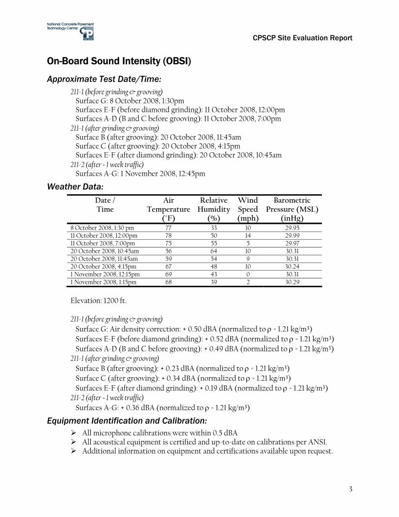
On-Board Sound Intensity (OBSI)
Approximate Test Date/Time: 211-1 (before grinding & grooving) Surface G: 8 October 2008, 1:30pm Surfaces E-F (before diamond grinding): 11 October 2008, 12:00pm Surfaces A-D (B and C before grooving): 11 October 2008, 7:00pm 211-1 (after grinding & grooving) Surface B (after grooving): 20 October 2008, 11:45am Surface C (after grooving): 20 October 2008, 4:15pm Surfaces E-F (after diamond grinding): 20 October 2008, 10:45am 211-2 (after ~ 1 week traffic) Surfaces A-G: 1 November 2008, 12:45pm
Weather Data: Date / Time
Air Temperature
(°F)
Relative Humidity
(%)
Wind Speed (mph)
Barometric Pressure (MSL)
(inHg) 8 October 2008, 1:30 pm 77 33 10 29.95 11 October 2008, 12:00pm 78 50 14 29.99 11 October 2008, 7:00pm 75 55 5 29.97 20 October 2008, 10:45am 56 64 10 30.31 20 October 2008, 11:45am 59 54 9 30.31 20 October 2008, 4:15pm 67 48 10 30.24 1 November 2008, 12:15pm 69 43 0 30.31 1 November 2008, 1:15pm 68 39 2 30.29
Elevation: 1200 ft. 211-1 (before grinding & grooving) Surface G: Air density correction: + 0.50 dBA (normalized to ρ = 1.21 kg/m³) Surfaces E-F (before diamond grinding): + 0.52 dBA (normalized to ρ = 1.21 kg/m³) Surfaces A-D (B and C before grooving): + 0.49 dBA (normalized to ρ = 1.21 kg/m³) 211-1 (after grinding & grooving) Surface B (after grooving): + 0.23 dBA (normalized to ρ = 1.21 kg/m³) Surface C (after grooving): + 0.34 dBA (normalized to ρ = 1.21 kg/m³) Surfaces E-F (after diamond grinding): + 0.19 dBA (normalized to ρ = 1.21 kg/m³) 211-2 (after ~ 1 week traffic) Surfaces A-G: + 0.36 dBA (normalized to ρ = 1.21 kg/m³)
Equipment Identification and Calibration: All microphone calibrations were within 0.5 dBA All acoustical equipment is certified and up-to-date on calibrations per ANSI. Additional information on equipment and certifications available upon request.
CPSCP Site Evaluation Report
4
Site Condition: No free moisture present on surface. Pavement reasonably free of loose debris. No large objects within 2 ft. of pavement edge. Large radius (superelevated) horizontal curvature for Surface F. No significant grade changes. Crossfall appears typical for this type of roadway. For 211-1 (before grinding & grooving), surfaces were approximately 2-4 weeks
old, and had not yet been opened to (public) traffic. For 211-1 (after grinding & grooving), surfaces were approximately 4-6 weeks
old, and had not yet been opened to (public) traffic. Excess fin height on areas of the conventional diamond ground surfaces was evident. Ground surfaces appear “dusty/dirty”.
For 211-2 (after ~ 1 week traffic), surfaces were approximately 6-8 weeks old, and had less than one week of traffic. Excess fin height on areas of the conventional diamond ground surfaces was still evident. Ground surfaces appeared clean (free of dust/dirt).
Patching operations were ongoing during testing, making deviations from right wheel path necessary at some locations.
Pavement Temperatures: 211-1 (before grinding & grooving) Surface G (8 Oct): 81 to 84°F Surfaces E-F (before diamond grinding, 11 Oct): 82 to 83°F 211-1 (after grinding & grooving) Surfaces E-F (after diamond grinding, 20 Oct): 63°F Surface B (after grooving, 20 Oct): 63°F Surface C (after grooving, 20 Oct): 69 to 70°F 211-2 (after ~ 1 week traffic) Surfaces A-G: 66 to 76°F

CPSCP Site Evaluation Report
5
Test Vehicle: 2003 Buick Century
Test Tire: ASTM F 2493 Standard Reference Test Tire (SRTT) Cold Inflation Pressure: 30 psi
Nominal Test Speed: 60 mph
Representative Photographs:
Figure 2: Surface A – Longitudinal Tining.
Figure 3: Surface B – Longitudinal Grooving + Burlap Drag (photo/test before grooving).
CPSCP Site Evaluation Report
6
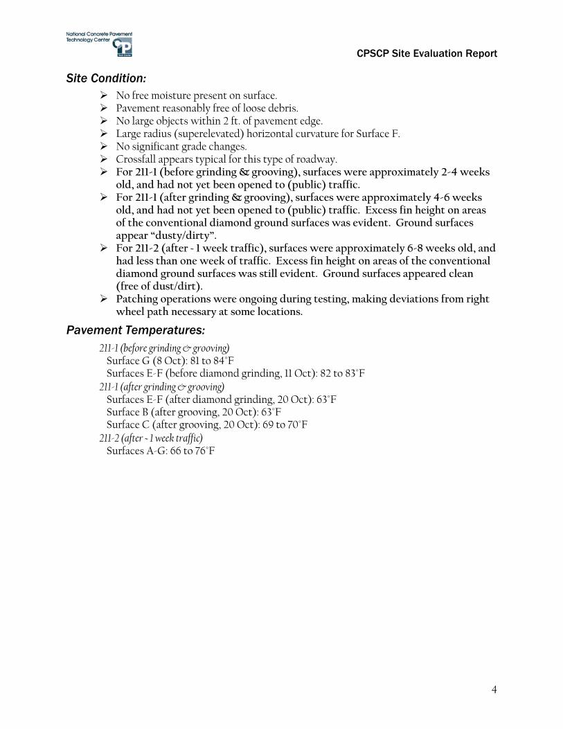
Figure 4: Surface B – Longitudinal Grooving + Burlap Drag (photo/test after grooving).
Figure 5: Surface C – Longitudinal Grooving + Turf Drag (photo/test before grooving).
Figure 6: Surface C – Longitudinal Grooving + Turf Drag (photo/test after grooving).
CPSCP Site Evaluation Report
7
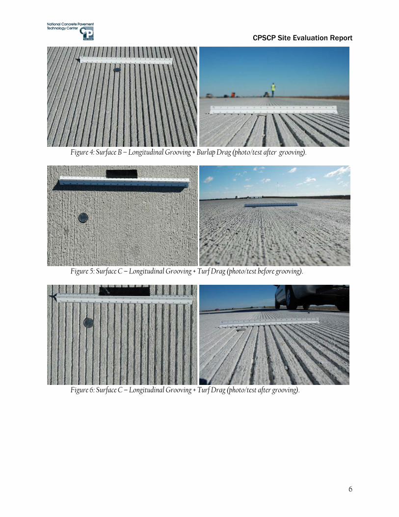
Figure 7: Surface D –Turf Drag.
Figure 8: Surface E – Conventional Diamond Grinding (photo/test before grinding).
Figure 9: Surface E – Conventional Diamond Grinding (photo/test after grinding).
CPSCP Site Evaluation Report
8
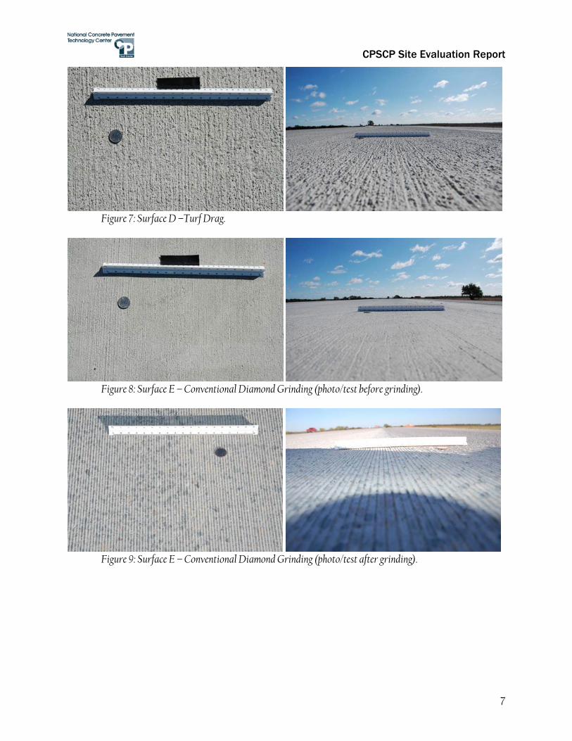
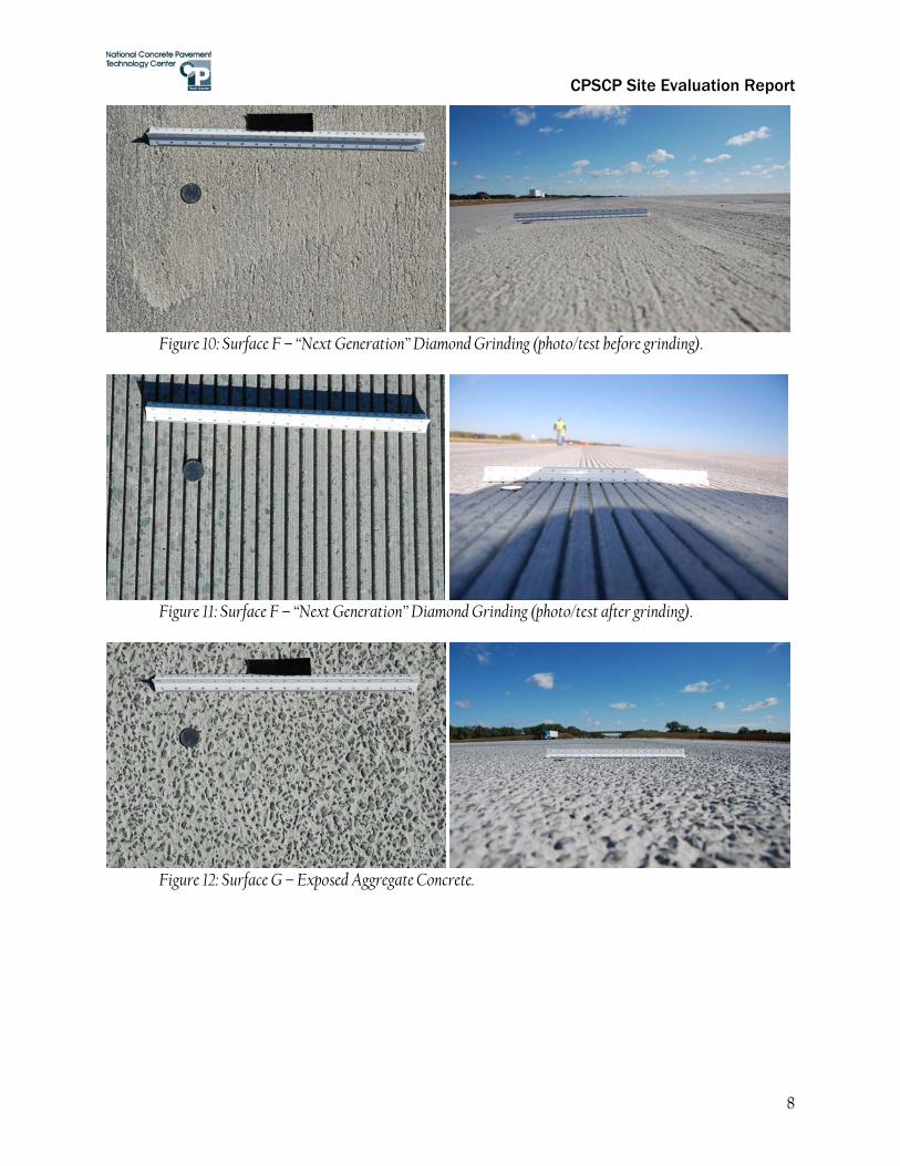
Figure 10: Surface F – “Next Generation” Diamond Grinding (photo/test before grinding).
Figure 11: Surface F – “Next Generation” Diamond Grinding (photo/test after grinding).
Figure 12: Surface G – Exposed Aggregate Concrete.
CPSCP Site Evaluation Report
9
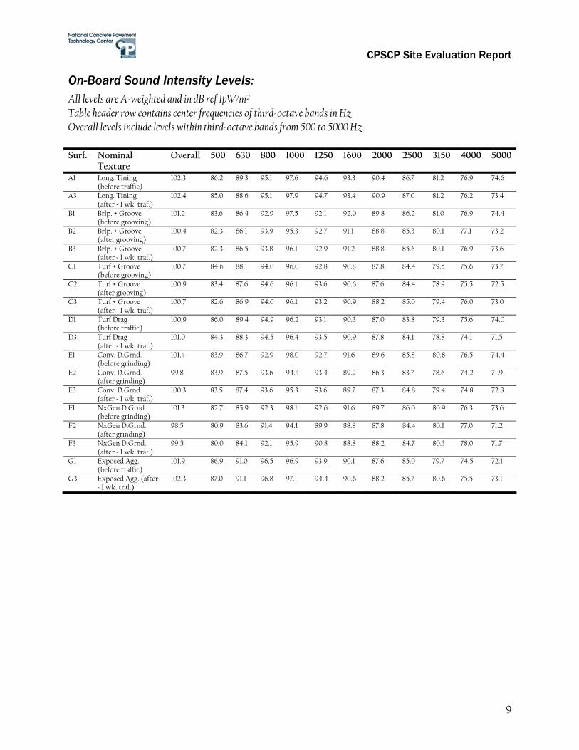
On-Board Sound Intensity Levels: All levels are A-weighted and in dB ref 1pW/m² Table header row contains center frequencies of third-octave bands in Hz Overall levels include levels within third-octave bands from 500 to 5000 Hz Surf. Nominal
Texture Overall 500 630 800 1000 1250 1600 2000 2500 3150 4000 5000
A1 Long. Tining (before traffic)
102.3 86.2 89.3 95.1 97.6 94.6 93.3 90.4 86.7 81.2 76.9 74.6
A3 Long. Tining (after ~ 1 wk. traf.)
102.4 85.0 88.6 95.1 97.9 94.7 93.4 90.9 87.0 81.2 76.2 73.4
B1 Brlp. + Groove (before grooving)
101.2 83.6 86.4 92.9 97.5 92.1 92.0 89.8 86.2 81.0 76.9 74.4
B2 Brlp. + Groove (after grooving)
100.4 82.3 86.1 93.9 95.3 92.7 91.1 88.8 85.3 80.1 77.1 73.2
B3 Brlp. + Groove (after ~ 1 wk. traf.)
100.7 82.3 86.5 93.8 96.1 92.9 91.2 88.8 85.6 80.1 76.9 73.6
C1 Turf + Groove (before grooving)
100.7 84.6 88.1 94.0 96.0 92.8 90.8 87.8 84.4 79.5 75.6 73.7
C2 Turf + Groove (after grooving)
100.9 83.4 87.6 94.6 96.1 93.6 90.6 87.6 84.4 78.9 75.5 72.5
C3 Turf + Groove (after ~ 1 wk. traf.)
100.7 82.6 86.9 94.0 96.1 93.2 90.9 88.2 85.0 79.4 76.0 73.0
D1 Turf Drag (before traffic)
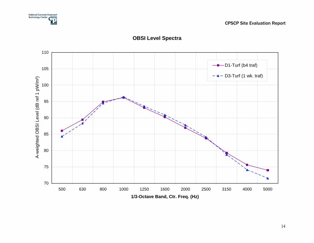
100.9 86.0 89.4 94.9 96.2 93.1 90.3 87.0 83.8 79.3 75.6 74.0
D3 Turf Drag (after ~ 1 wk. traf.)
101.0 84.3 88.3 94.5 96.4 93.5 90.9 87.8 84.1 78.8 74.1 71.5
E1 Conv. D.Grnd. (before grinding)
101.4 83.9 86.7 92.9 98.0 92.7 91.6 89.6 85.8 80.8 76.5 74.4
E2 Conv. D.Grnd. (after grinding)
99.8 83.9 87.5 93.6 94.4 93.4 89.2 86.3 83.7 78.6 74.2 71.9
E3 Conv. D.Grnd. (after ~ 1 wk. traf.)
100.3 83.5 87.4 93.6 95.3 93.6 89.7 87.3 84.8 79.4 74.8 72.8
F1 NxGen D.Grnd. (before grinding)
101.3 82.7 85.9 92.3 98.1 92.6 91.6 89.7 86.0 80.9 76.3 73.6
F2 NxGen D.Grnd. (after grinding)
98.5 80.9 83.6 91.4 94.1 89.9 88.8 87.8 84.4 80.1 77.0 71.2
F3 NxGen D.Grnd. (after ~ 1 wk. traf.)
99.5 80.0 84.1 92.1 95.9 90.8 88.8 88.2 84.7 80.3 78.0 71.7
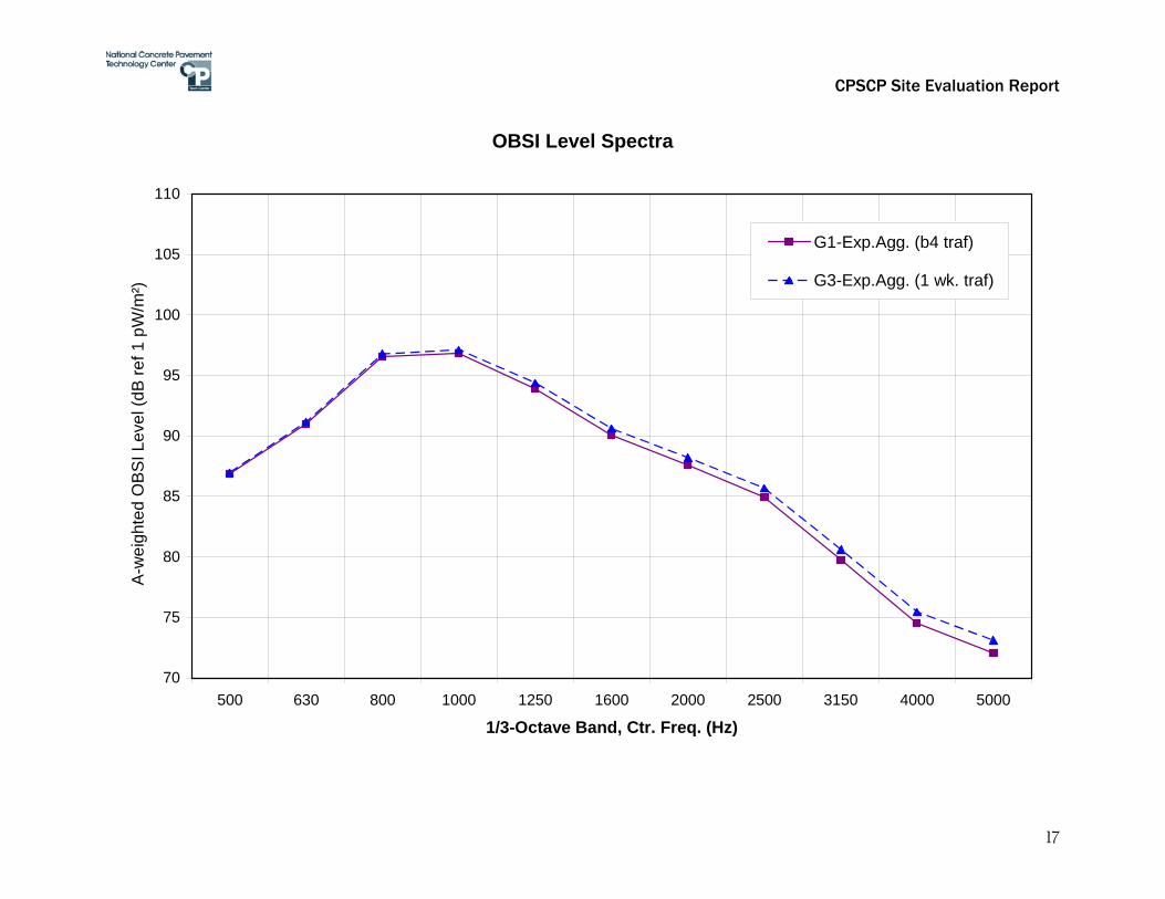
G1 Exposed Agg. (before traffic)
101.9 86.9 91.0 96.5 96.9 93.9 90.1 87.6 85.0 79.7 74.5 72.1
G3 Exposed Agg. (after ~ 1 wk. traf.)
102.3 87.0 91.1 96.8 97.1 94.4 90.6 88.2 85.7 80.6 75.5 73.1
CPSCP Site Evaluation Report
10
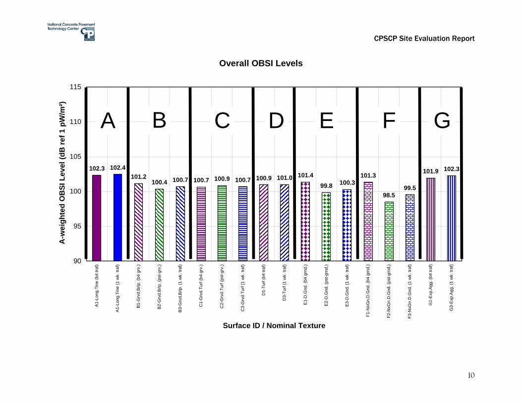
Overall OBSI Levels
102.3 102.4101.2
100.4 100.7 100.7 100.9 100.7 100.9 101.0 101.499.8 100.3
101.3
98.599.5
101.9 102.3
90
95
100
105
110
115A
1-Lo
ng.T
ine
(b4
traf)
A1-
Long
.Tin
e (1
wk.
traf
)
B1-
Grv
d.B
rlp. (
b4 g
rv.)
B2-
Grv
d.B
rlp. (
pst-g
rv.)
B3-
Grv
d.B
rlp. (
1 w
k. tr
af)
C1-
Grv
d.Tu
rf (b
4 gr
v.)
C2-
Grv
d.Tu
rf (p
st-g
rv.)
C3-
Grv
d.Tu
rf (1
wk.
traf
)
D1-
Turf
(b4
traf)
D3-
Turf
(1 w
k. tr
af)
E1-
D.G
nd. (
b4 g
rnd.
)
E2-
D.G
nd. (
pst-g
rnd.
)
E3-
D.G
nd. (
1 w
k. tr
af)
F1-N
xGn.
D.G
nd. (
b4 g
rnd.
)
F2-N
xGn.
D.G
nd. (
pst-g
rnd.
)
F3-N
xGn.
D.G
nd. (
1 w
k. tr
af)
G1-
Exp
.Agg
. (b4
traf
)
G3-
Exp
.Agg
. (1
wk.
traf
)
Surface ID / Nominal Texture
A-w
eigh
ted
OB
SI L
evel
(dB
ref 1
pW
/m²)
A B C D E F G
CPSCP Site Evaluation Report
11
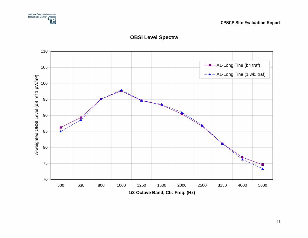
OBSI Level Spectra
70
75
80
85
90
95
100
105
110
500 630 800 1000 1250 1600 2000 2500 3150 4000 5000
1/3-Octave Band, Ctr. Freq. (Hz)
A-w
eigh
ted
OB
SI L
evel
(dB
ref 1
pW
/m²)
A1-Long.Tine (b4 traf)
A1-Long.Tine (1 wk. traf)
CPSCP Site Evaluation Report
12
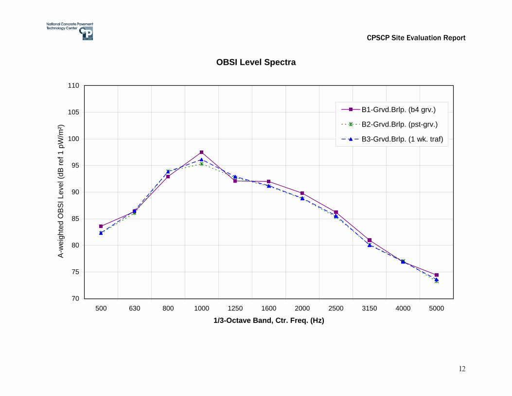
OBSI Level Spectra
70
75
80
85
90
95
100
105
110
500 630 800 1000 1250 1600 2000 2500 3150 4000 5000
1/3-Octave Band, Ctr. Freq. (Hz)
A-w
eigh
ted
OB
SI L
evel
(dB
ref 1
pW
/m²)
B1-Grvd.Brlp. (b4 grv.)
B2-Grvd.Brlp. (pst-grv.)
B3-Grvd.Brlp. (1 wk. traf)

CPSCP Site Evaluation Report
13
OBSI Level Spectra
70
75
80
85
90
95
100
105
110
500 630 800 1000 1250 1600 2000 2500 3150 4000 5000
1/3-Octave Band, Ctr. Freq. (Hz)
A-w
eigh
ted
OB
SI L
evel
(dB
ref 1
pW
/m²)
C1-Grvd.Turf (b4 grv.)
C2-Grvd.Turf (pst-grv.)
C3-Grvd.Turf (1 wk. traf)
CPSCP Site Evaluation Report
14
OBSI Level Spectra
70
75
80
85
90
95
100
105
110
500 630 800 1000 1250 1600 2000 2500 3150 4000 5000
1/3-Octave Band, Ctr. Freq. (Hz)
A-w
eigh
ted
OB
SI L
evel
(dB
ref 1
pW
/m²)
D1-Turf (b4 traf)
D3-Turf (1 wk. traf)

CPSCP Site Evaluation Report
15
OBSI Level Spectra
70
75
80
85
90
95
100
105
110
500 630 800 1000 1250 1600 2000 2500 3150 4000 5000
1/3-Octave Band, Ctr. Freq. (Hz)
A-w
eigh
ted
OB
SI L
evel
(dB
ref 1
pW
/m²)
E1-D.Gnd. (b4 grnd.)
E2-D.Gnd. (pst-grnd.)
E3-D.Gnd. (1 wk. traf)

CPSCP Site Evaluation Report
16
OBSI Level Spectra
70
75
80
85
90
95
100
105
110
500 630 800 1000 1250 1600 2000 2500 3150 4000 5000
1/3-Octave Band, Ctr. Freq. (Hz)
A-w
eigh
ted
OB
SI L
evel
(dB
ref 1
pW
/m²)
F1-NxGn.D.Gnd. (b4 grnd.)
F2-NxGn.D.Gnd. (pst-grnd.)
F3-NxGn.D.Gnd. (1 wk. traf)
CPSCP Site Evaluation Report
17
OBSI Level Spectra
70
75
80
85
90
95
100
105
110
500 630 800 1000 1250 1600 2000 2500 3150 4000 5000
1/3-Octave Band, Ctr. Freq. (Hz)
A-w
eigh
ted
OB
SI L
evel
(dB
ref 1
pW
/m²)
G1-Exp.Agg. (b4 traf)
G3-Exp.Agg. (1 wk. traf)

CPSCP Site Evaluation Report
18
Spatial Variability of OBSI Levels
94
96
98
100
102
104
106
108
110
0 100 200 300 400 500
Distance (m)
A-w
eigh
ted
OBS
I Lev
el (d
B re
f 1 p
W/m
²), 0
.5 s
ec M
vngA
vg A1-Long.Tine (b4 traf)A1-Long.Tine (1 wk. traf)
CPSCP Site Evaluation Report
19
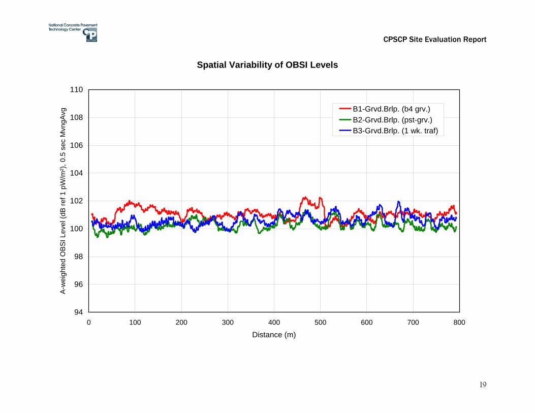
Spatial Variability of OBSI Levels
94
96
98
100
102
104
106
108
110
0 100 200 300 400 500 600 700 800
Distance (m)
A-w
eigh
ted
OBS
I Lev
el (d
B re
f 1 p
W/m
²), 0
.5 s
ec M
vngA
vg B1-Grvd.Brlp. (b4 grv.)B2-Grvd.Brlp. (pst-grv.)B3-Grvd.Brlp. (1 wk. traf)
CPSCP Site Evaluation Report
20
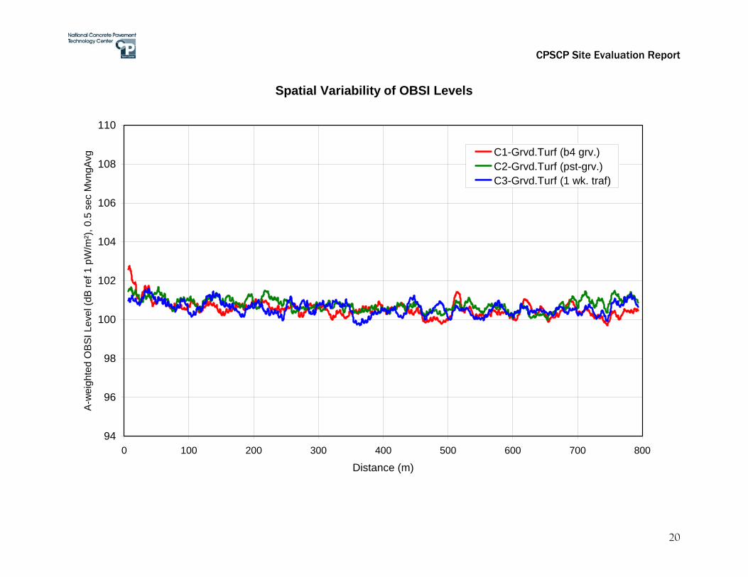
Spatial Variability of OBSI Levels
94
96
98
100
102
104
106
108
110
0 100 200 300 400 500 600 700 800
Distance (m)
A-w
eigh
ted
OBS
I Lev
el (d
B re
f 1 p
W/m
²), 0
.5 s
ec M
vngA
vg C1-Grvd.Turf (b4 grv.)C2-Grvd.Turf (pst-grv.)C3-Grvd.Turf (1 wk. traf)

CPSCP Site Evaluation Report
21
Spatial Variability of OBSI Levels
94
96
98
100
102
104
106
108
110
0 100 200 300 400 500 600
Distance (m)
A-w
eigh
ted
OBS
I Lev
el (d
B re
f 1 p
W/m
²), 0
.5 s
ec M
vngA
vg D1-Turf (b4 traf)D3-Turf (1 wk. traf)

CPSCP Site Evaluation Report
22
Spatial Variability of OBSI Levels
94
96
98
100
102
104
106
108
110
0 100 200 300 400 500 600 700 800
Distance (m)
A-w
eigh
ted
OBS
I Lev
el (d
B re
f 1 p
W/m
²), 0
.5 s
ec M
vngA
vg
E1-D.Gnd. (b4 grnd.)E2-D.Gnd. (pst-grnd.)E3-D.Gnd. (1 wk. traf)

CPSCP Site Evaluation Report
23
Spatial Variability of OBSI Levels
94
96
98
100
102
104
106
108
110
0 100 200 300 400 500 600 700 800
Distance (m)
A-w
eigh
ted
OBS
I Lev
el (d
B re
f 1 p
W/m
²), 0
.5 s
ec M
vngA
vg
F1-NxGn.D.Gnd. (b4 grnd.)F2-NxGn.D.Gnd. (pst-grnd.)F3-NxGn.D.Gnd. (1 wk. traf)

CPSCP Site Evaluation Report
24
Spatial Variability of OBSI Levels
94
96
98
100
102
104
106
108
110
0 100 200 300 400 500 600 700 800 900 1000
Distance (m)
A-w
eigh
ted
OBS
I Lev
el (d
B re
f 1 p
W/m
²), 0
.5 s
ec M
vngA
vg G1-Exp.Agg. (b4 traf)G3-Exp.Agg. (1 wk. traf)

CPSCP Site Evaluation Report
25
Cumulative Distribution of OBSI Levels
0%
10%
20%
30%
40%
50%
60%
70%
80%
90%
100%
97 98 99 100 101 102 103 104 105
A-weighted OBSI Level (dB ref 1 pW/m²), 0.5 sec MvngAvg
Cum
ulat
ive
%
A1-Long.Tine (b4 traf)A1-Long.Tine (1 wk. traf)
CPSCP Site Evaluation Report
26
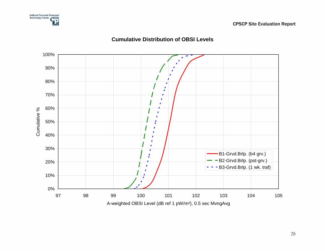
Cumulative Distribution of OBSI Levels
0%
10%
20%
30%
40%
50%
60%
70%
80%
90%
100%
97 98 99 100 101 102 103 104 105
A-weighted OBSI Level (dB ref 1 pW/m²), 0.5 sec MvngAvg
Cum
ulat
ive
%
B1-Grvd.Brlp. (b4 grv.)B2-Grvd.Brlp. (pst-grv.)B3-Grvd.Brlp. (1 wk. traf)
CPSCP Site Evaluation Report
27
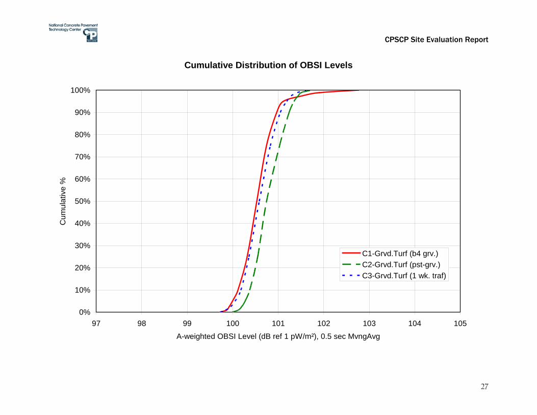
Cumulative Distribution of OBSI Levels
0%
10%
20%
30%
40%
50%
60%
70%
80%
90%
100%
97 98 99 100 101 102 103 104 105
A-weighted OBSI Level (dB ref 1 pW/m²), 0.5 sec MvngAvg
Cum
ulat
ive
%
C1-Grvd.Turf (b4 grv.)C2-Grvd.Turf (pst-grv.)C3-Grvd.Turf (1 wk. traf)

CPSCP Site Evaluation Report
28
Cumulative Distribution of OBSI Levels
0%
10%
20%
30%
40%
50%
60%
70%
80%
90%
100%
97 98 99 100 101 102 103 104 105
A-weighted OBSI Level (dB ref 1 pW/m²), 0.5 sec MvngAvg
Cum
ulat
ive
%
D1-Turf (b4 traf)D3-Turf (1 wk. traf)
CPSCP Site Evaluation Report
29
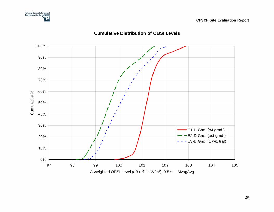
Cumulative Distribution of OBSI Levels
0%
10%
20%
30%
40%
50%
60%
70%
80%
90%
100%
97 98 99 100 101 102 103 104 105
A-weighted OBSI Level (dB ref 1 pW/m²), 0.5 sec MvngAvg
Cum
ulat
ive
%
E1-D.Gnd. (b4 grnd.)E2-D.Gnd. (pst-grnd.)E3-D.Gnd. (1 wk. traf)
CPSCP Site Evaluation Report
30
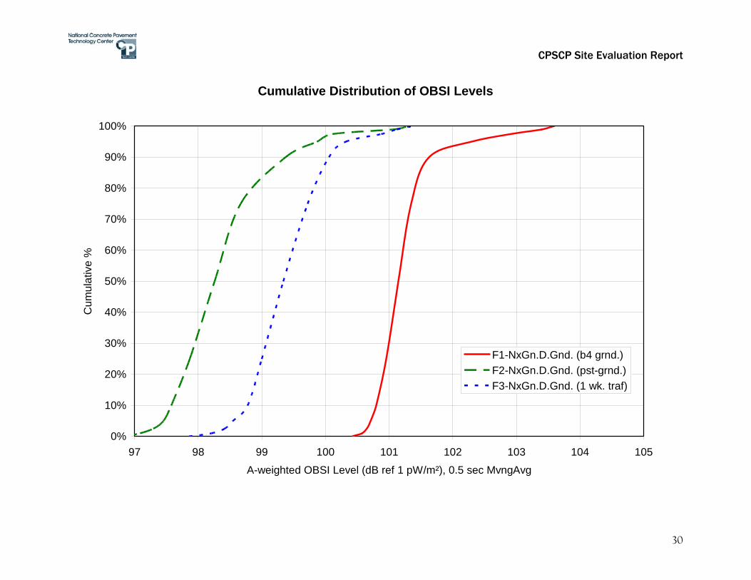
Cumulative Distribution of OBSI Levels
0%
10%
20%
30%
40%
50%
60%
70%
80%
90%
100%
97 98 99 100 101 102 103 104 105
A-weighted OBSI Level (dB ref 1 pW/m²), 0.5 sec MvngAvg
Cum
ulat
ive
%
F1-NxGn.D.Gnd. (b4 grnd.)F2-NxGn.D.Gnd. (pst-grnd.)F3-NxGn.D.Gnd. (1 wk. traf)

CPSCP Site Evaluation Report
31
Cumulative Distribution of OBSI Levels
0%
10%
20%
30%
40%
50%
60%
70%
80%
90%
100%
97 98 99 100 101 102 103 104 105
A-weighted OBSI Level (dB ref 1 pW/m²), 0.5 sec MvngAvg
Cum
ulat
ive
%
G1-Exp.Agg. (b4 traf)G3-Exp.Agg. (1 wk. traf)

CPSCP Site Evaluation Report
A-1
Appendix A: Overview of Typical OBSI Levels for Concrete Pavements
With respect to tire-pavement noise, Figure A-1 illustrates the range of noise levels that have been measured on the hundreds of pavements to date under the CPSCP. The population of pavements is categorized by nominal texture type – and is shown as normalized distributions of the measured noise levels.
0.00
0.05
0.10
0.15
0.20
0.25
0.30
96 98 100 102 104 106 108 110A-weighted Overall OBSI Level, 60 mph, SRTT (dB ref 1 pW/m²)
Prob
abili
ty D
ensi
ty
Diamond Grinding
Drag
Longitudinal Tining
Transverse Tining
Figure A-1: Normalized distributions of OBSI noise levels for conventional concrete pavement textures. Based on this information, it is important that the highway community establish rational goals for noise. Based on the work conducted to date, an A-weighted tire-pavement noise level of 100 dB (ref 1pW/m²) measured using On-Board Sound Intensity with the SRTT test tire at 60 mph appears to be a reasonable target threshold [1,2,3]. With this in mind, and referring to Figure A-1, the following can be concluded:
50% (half) of all conventionally diamond ground surfaces that were measured already meet this goal;
25% (1 out of every 4) drag textures meet this goal; 12% (1 out of every 8) longitudinally tined surfaces meet this goal; and 4% (1 out of every 25) transversely tined surfaces meet this goal; however, nominal
tine spacings are all at or less than 1/2 inch.
CPSCP Site Evaluation Report
A-2
It should also be noted that since this population includes pavements at all different stages of their service lives, newer concrete surfaces – those measured shortly after opening to traffic – will typically measure even quieter, and thus higher percentages of these pavements will meet the target OBSI threshold of 100 dBA. From this information, it can be concluded that virtually all conventional nominal textures have the potential to be constructed as quieter concrete surfaces. What are currently being developed under the CPSCP are the better practices for design and construction that will increase the probability of this occurring.
References 1. Cackler, E.T., et. al., Concrete Pavement Surface Characteristics: Evaluation of Current Methods for
Controlling Tire-Pavement Noise, Final Report of FHWA Cooperative Agreement DTFH61-01-X-00042, Project 15, 2006.
2. Ferragut, T., Rasmussen, R.O., Wiegand, P., Mun, E., and E.T. Cackler, ISU-FHWA-ACPA Concrete Pavement Surface Characteristics Program Part 2: Preliminary Field Data Collection, National Concrete Pavement Technology Center Report DTFH61-01-X-00042 (Project 15, Part 2), 2007.
3. Rasmussen, R.O., et. al., How to Reduce Tire-Pavement Noise: Interim Better Practices for Constructing and Texturing Concrete Pavement Surfaces, National CP Technology Center Report, July 2008.
CPSCP Site Evaluation Report
B-1
Appendix B: Overview of the CPSCP
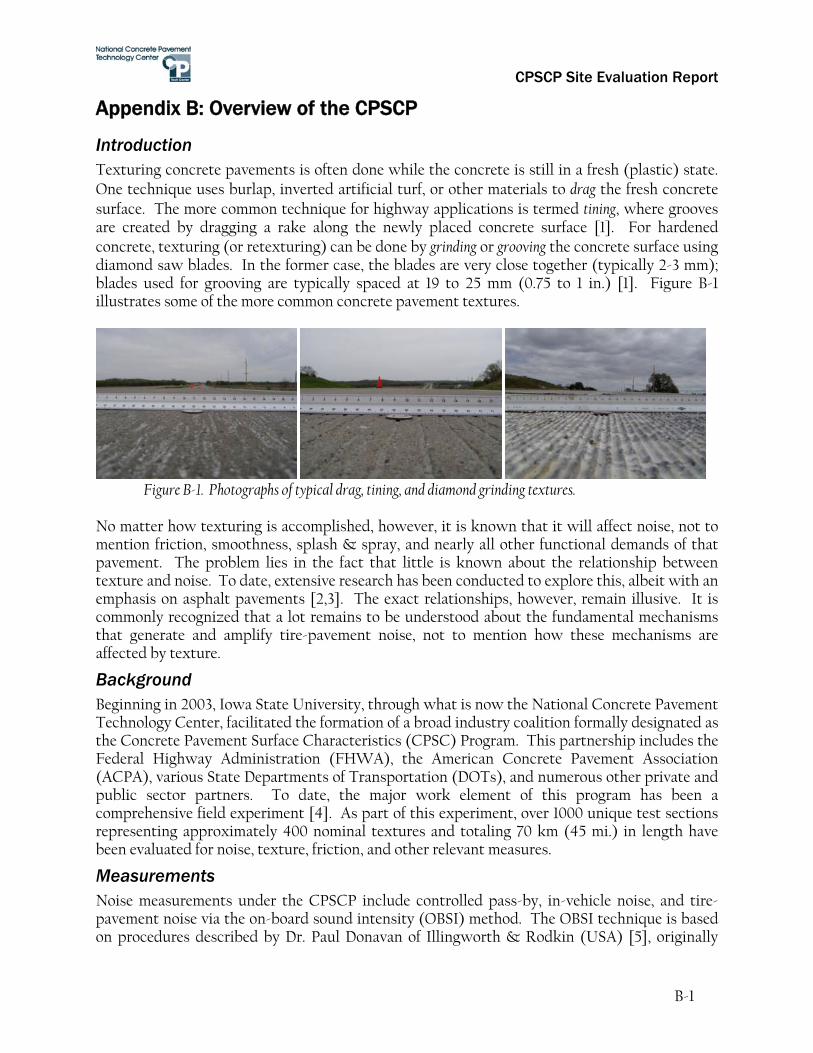
Introduction Texturing concrete pavements is often done while the concrete is still in a fresh (plastic) state. One technique uses burlap, inverted artificial turf, or other materials to drag the fresh concrete surface. The more common technique for highway applications is termed tining, where grooves are created by dragging a rake along the newly placed concrete surface [1]. For hardened concrete, texturing (or retexturing) can be done by grinding or grooving the concrete surface using diamond saw blades. In the former case, the blades are very close together (typically 2-3 mm); blades used for grooving are typically spaced at 19 to 25 mm (0.75 to 1 in.) [1]. Figure B-1 illustrates some of the more common concrete pavement textures.
Figure B-1. Photographs of typical drag, tining, and diamond grinding textures.
No matter how texturing is accomplished, however, it is known that it will affect noise, not to mention friction, smoothness, splash & spray, and nearly all other functional demands of that pavement. The problem lies in the fact that little is known about the relationship between texture and noise. To date, extensive research has been conducted to explore this, albeit with an emphasis on asphalt pavements [2,3]. The exact relationships, however, remain illusive. It is commonly recognized that a lot remains to be understood about the fundamental mechanisms that generate and amplify tire-pavement noise, not to mention how these mechanisms are affected by texture.
Background Beginning in 2003, Iowa State University, through what is now the National Concrete Pavement Technology Center, facilitated the formation of a broad industry coalition formally designated as the Concrete Pavement Surface Characteristics (CPSC) Program. This partnership includes the Federal Highway Administration (FHWA), the American Concrete Pavement Association (ACPA), various State Departments of Transportation (DOTs), and numerous other private and public sector partners. To date, the major work element of this program has been a comprehensive field experiment [4]. As part of this experiment, over 1000 unique test sections representing approximately 400 nominal textures and totaling 70 km (45 mi.) in length have been evaluated for noise, texture, friction, and other relevant measures.
Measurements Noise measurements under the CPSCP include controlled pass-by, in-vehicle noise, and tire-pavement noise via the on-board sound intensity (OBSI) method. The OBSI technique is based on procedures described by Dr. Paul Donavan of Illingworth & Rodkin (USA) [5], originally
CPSCP Site Evaluation Report
B-2
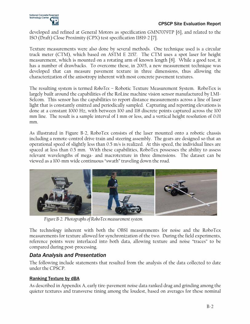
developed and refined at General Motors as specification GMN7079TP [6], and related to the ISO (Draft) Close Proximity (CPX) test specification 11819-2 [7]. Texture measurements were also done by several methods. One technique used is a circular track meter (CTM), which based on ASTM E 2157. The CTM uses a spot laser for height measurement, which is mounted on a rotating arm of known length [8]. While a good test, it has a number of drawbacks. To overcome these, in 2005, a new measurement technique was developed that can measure pavement texture in three dimensions, thus allowing the characterization of the anisotropy inherent with most concrete pavement textures. The resulting system is termed RoboTex – Robotic Texture Measurement System. RoboTex is largely built around the capabilities of the RoLine machine vision sensor manufactured by LMI-Selcom. This sensor has the capabilities to report distance measurements across a line of laser light that is constantly emitted and periodically sampled. Capturing and reporting elevations is done at a constant 1000 Hz, with between 100 and 118 discrete points captured across the 100 mm line. The result is a sample interval of 1 mm or less, and a vertical height resolution of 0.01 mm. As illustrated in Figure B-2, RoboTex consists of the laser mounted onto a robotic chassis including a remote-control drive train and steering assembly. The gears are designed so that an operational speed of slightly less than 0.5 m/s is realized. At this speed, the individual lines are spaced at less than 0.5 mm. With these capabilities, RoboTex possesses the ability to assess relevant wavelengths of mega- and macrotexture in three dimensions. The dataset can be viewed as a 100-mm wide continuous “swath” traveling down the road.
Figure B-2. Photographs of RoboTex measurement system.
The technology inherent with both the OBSI measurements for noise and the RoboTex measurements for texture allowed for synchronization of the two. During the field experiments, reference points were interlaced into both data, allowing texture and noise “traces” to be compared during post-processing.
Data Analysis and Presentation The following include statements that resulted from the analysis of the data collected to date under the CPSCP.
Ranking Texture by dBA
As described in Appendix A, early tire-pavement noise data ranked drag and grinding among the quieter textures and transverse tining among the loudest, based on averages for these nominal

CPSCP Site Evaluation Report
B-3
texture types. However, there are many texture subsets within each class. This general ranking does not always hold true, especially given the variability that is present. Rank ordering to date has been based in large part on sound levels measured near the tire-pavement source, using OBSI. Rank ordering by sound level as received wayside will likely be similar, however, as work by Dr. Paul Donavan and Caltrans has demonstrated [5]
OBSI Ranges
Measured tire-pavement noise levels for concrete pavements range from 97 dBA on the low end to over 110 dBA on the high end. It should be noted that a 10 dBA level change can be illustrated as a “doubling” of perceived sound (albeit this is generally true for the same type of sound). Based on the data collected to date, this range of noise values is likely representative of the total population of concrete pavements in the country. While there may outliers on the high end, the 97 dBA level is likely be close to the lowest possible for concrete pavements using conventional technology (i.e., dense concrete, as opposed to porous/pervious).
Texture Geometry
In the early stages of analysis, there at first appeared to be a relationship between texture depth and tire-pavement noise. However, this is an oversimplification and was quickly dismissed, as it falls short of truly characterizing the relationship between texture and noise. The correlation that does sometimes appear is likely to have more to do with the fact that a deeper (more aggressive) texture causes more disturbances of the concrete surface, and thus leads to random deposits of concrete on the surface that, in turn, increase noise. Characterizing the exact relationship between texture and noise is an ongoing task under the CPSCP. While trends are evident, there are sometimes exceptions, which underscore the need for a more fundamental model. One issue is the need to establish better indices for describing texture. Spectral analysis of the texture, for example, coupled with the texture skew (bias), has revealed a lot more clarity in these relationships.
Wear Rate
Analysis of the data to date have shown that early wear on textures (when opened to traffic) will often lead to a 1 to 2 dBA decrease in tire-pavement noise. With traffic volume as only one variable, snow plowing and other environmental effects appear to also be impacting the wear as well. Once this initial change has occurred, however, there is typically an increase in noise level over time, as the texture will change under traffic and due to the climate and maintenance activities. The rate of change is a function of both the texture configuration and the quality of the concrete, among numerous other factors.
Better Practices for Design and Construction The current emphasis of the CPSCP is the development of guidelines for the design and construction of quieter concrete pavements that do not compromise on safety, durability, or cost. Better practices are currently under review by the highway community. In the process of developing these guidelines, the following steps were considered as a guide:
1. Recognize what properties of a pavement surface make it quiet (and what make it loud);
CPSCP Site Evaluation Report
B-4
2. Design the pavement surface in such a way to avoid those adverse properties; 3. Construct the pavement surface to also avoid those adverse properties, but also in a
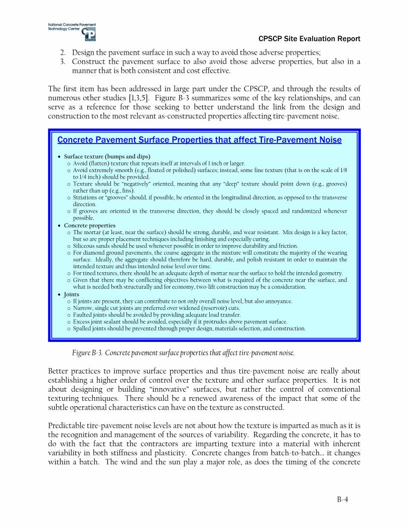
manner that is both consistent and cost effective. The first item has been addressed in large part under the CPSCP, and through the results of numerous other studies [1,3,5]. Figure B-3 summarizes some of the key relationships, and can serve as a reference for those seeking to better understand the link from the design and construction to the most relevant as-constructed properties affecting tire-pavement noise.
Figure B-3. Concrete pavement surface properties that affect tire-pavement noise. Better practices to improve surface properties and thus tire-pavement noise are really about establishing a higher order of control over the texture and other surface properties. It is not about designing or building “innovative” surfaces, but rather the control of conventional texturing techniques. There should be a renewed awareness of the impact that some of the subtle operational characteristics can have on the texture as constructed. Predictable tire-pavement noise levels are not about how the texture is imparted as much as it is the recognition and management of the sources of variability. Regarding the concrete, it has to do with the fact that the contractors are imparting texture into a material with inherent variability in both stiffness and plasticity. Concrete changes from batch-to-batch… it changes within a batch. The wind and the sun play a major role, as does the timing of the concrete
Concrete Pavement Surface Properties that affect Tire-Pavement Noise • Surface texture (bumps and dips)
o Avoid (flatten) texture that repeats itself at intervals of 1 inch or larger. o Avoid extremely smooth (e.g., floated or polished) surfaces; instead, some fine texture (that is on the scale of 1/8
to 1/4 inch) should be provided. o Texture should be “negatively” oriented, meaning that any “deep” texture should point down (e.g., grooves)
rather than up (e.g., fins). o Striations or “grooves” should, if possible, be oriented in the longitudinal direction, as opposed to the transverse
direction. o If grooves are oriented in the transverse direction, they should be closely spaced and randomized whenever
possible. • Concrete properties
o The mortar (at least, near the surface) should be strong, durable, and wear resistant. Mix design is a key factor, but so are proper placement techniques including finishing and especially curing.
o Siliceous sands should be used whenever possible in order to improve durability and friction. o For diamond ground pavements, the coarse aggregate in the mixture will constitute the majority of the wearing
surface. Ideally, the aggregate should therefore be hard, durable, and polish resistant in order to maintain the intended texture and thus intended noise level over time.
o For tined textures, there should be an adequate depth of mortar near the surface to hold the intended geometry. o Given that there may be conflicting objectives between what is required of the concrete near the surface, and
what is needed both structurally and for economy, two-lift construction may be a consideration. • Joints
o If joints are present, they can contribute to not only overall noise level, but also annoyance. o Narrow, single cut joints are preferred over widened (reservoir) cuts. o Faulted joints should be avoided by providing adequate load transfer. o Excess joint sealant should be avoided, especially if it protrudes above pavement surface. o Spalled joints should be prevented through proper design, materials selection, and construction.

CPSCP Site Evaluation Report
B-5
mixing, transport, placement, and (eventually) the texturing and curing (the latter being important for acoustical durability). For today, we can promote better practices that focus our attention on what we should be doing better on today’s concrete spreads. For tomorrow, the solution will likely be automation of the texturing operation. Over the years, slipform concrete paving operations have become more and more automated. Automatic grade control, for example, is now a virtually standard feature for most slipform pavers. Monitoring of vibrator functionality and frequency is also common. Maybe the texturing operation is next. To meet the demands for predictable low-noise surfaces, automation will allow the paver, texture cart, and grinding operators to monitor the texture being produced, and make adjustments on the fly. Ultimately, this approach may be the best way to achieve a specified “target texture” on concrete pavements. For now, we can make significant improvements by simply adopting “better practices”.
References 1. U. Sandberg and J. Ejsmont, Tyre/Road Noise Reference Book. Informex, Handelsbolag,
Sweden, 2002. 2. R. Rasmussen, Y. Resendez, G. Chang, and T. Ferragut, Synthesis of Practice for the Control of
Tire-Pavement Noise using Concrete Pavements, Iowa State Univ., 2006. 3. Guidance manual for the implementation of low-noise road surfaces, FEHRL Report 2006/02, Ed.
by Phil Morgan, TRL, 2006. 4. T. Ferragut, R. Rasmussen, P. Wiegand, E. Mun, and E.T. Cackler, ISU-FHWA-ACPA
Concrete Pavement Surface Characteristics Program Part 2: Preliminary Field Data Collection, National Concrete Pavement Technology Center Report DTFH61-01-X-00042 (Project 15, Part 2), 2007.
5. P. Donavan and B. Rymer, “Quantification of Tire/Pavement Noise: Application of the Sound Intensity Method”, Proceedings of Inter-Noise 2004, Prague, the Czech Republic, 2004.
6. General Motors, “Road Tire Noise Evaluation Procedure,” Test Procedure GMN7079TP, 2004.
7. ISO, “Acoustics – Measurement of the influence of road surfaces on traffic noise – Part 2: The close proximity method,” ISO TC 43 / SC 1 N, ISO/CD 11819-2, 2000.
8. ASTM, “Standard Test Method for Measuring Pavement Macrotexture Properties using the Circular Track Meter,” Standard E 2157, 2001.

CPSCP Site Evaluation Report
C-1
Appendix C: The Little Book of Quieter Pavements
THE LITTLE BOOK OF QUIETER PAVEMENTS
U.S. Department of Transportation Federal Highway Administration
FHWA-IF-08-004 July 2007

Notice
This document is disseminated under the sponsorship of the Department of Transportation in the interest of information exchange. The United States Government assumes no liability for its contents or the use thereof. This report does not constitute a standard, specification, or regulation. The United States Government does not endorse products or manufacturers. Trade or manufacturer's names appear herein only because they are considered essential to the object of this document.

1. Report No. FHWA-IF-08-004
2. Government Accession No. N/A
3. Recipient's Catalog No. N/A
4. Title and Subtitle The Little Book of Quieter Pavements
5. Report Date July 2007
6. Performing Organization Code N/A
7. Author(s) Robert Otto Rasmussen, Robert J. Bernhard, Ulf Sandberg, Eric P. Mun
8. Performing Organization Report No.
9. Performing Organization Name and Address The Transtec Group, Inc. 6111 Balcones Drive Austin, Texas 78731
10. Work Unit No. (TRAIS) N/A 11. Contract or Grant No. DTFH61-04-D-00009, TO#9
12. Sponsoring Agency Name and Address Federal Highway Administration Office of Pavement Technology, HIPT-1 1200 New Jersey Avenue, SE Washington, DC 20590
13. Type of Report and Period Covered Final
14. Sponsoring Agency Code
15. Supplementary Notes Contracting Officer’s Technical Representatives: Mark Swanlund, HIPT-1; Mark Ferroni, HEPN-20
16. Abstract The idea of designing and building quieter pavements is not new, but in recent years there has been a groundswell of interest in making this a higher priority. Various State Highway Agencies and the Federal Highway Administration have responded accordingly with both research and implementation activities that both educate on the state-of-the-practice, and advance the state-of-the-art. The Little Book of Quieter Pavements was developed with this purpose in mind… to help educate the transportation industry, and in some cases the general public, about the numerous principles behind quieter pavements, and how they connect together.
17. Key Word Quieter pavements, tire-pavement noise, highway noise, close proximity, on-board sound intensity, CPX, OBSI, TNM, pass-by, wayside, SPB.
18. Distribution Statement No restrictions. This document is available to the public through: National Technical Information Service 5825 Port Royal Road Springfield, VA 22161
19. Security Classif. (of this report) Unclassified
20. Security Classif. (of this page) Unclassified
21. No. of Pages 37
22. Price
Form DOT F 1700.7 (8-72) Reproduction of completed page authorized
Technical Report Documentation Page
SI* (MODERN METRIC) CONVERSION FACTORS APPROXIMATE CONVERSIONS TO SI UNITS
Symbol When You Know Multiply By To Find Symbol LENGTH
in inches 25.4 millimeters mm ft feet 0.305 meters m yd yards 0.914 meters m mi miles 1.61 kilometers km
AREA in2 square inches 645.2 square millimeters mm2
ft2 square feet 0.093 square meters m2
yd2 square yard 0.836 square meters m2
ac acres 0.405 hectares hami2 square miles 2.59 square kilometers km2
VOLUME fl oz fluid ounces 29.57 milliliters mL gal gallons 3.785 liters L ft3 cubic feet 0.028 cubic meters m3
yd3 cubic yards 0.765 cubic meters m3
NOTE: volumes greater than 1000 L shall be shown in m3
MASS oz ounces 28.35 grams glb pounds 0.454 kilograms kgT short tons (2000 lb) 0.907 megagrams (or "metric ton") Mg (or "t")
TEMPERATURE (exact degrees) oF Fahrenheit 5 (F-32)/9 Celsius oC
or (F-32)/1.8 ILLUMINATION
fc foot-candles 10.76 lux lxfl foot-Lamberts 3.426 candela/m2 cd/m2
FORCE and PRESSURE or STRESS lbf poundforce 4.45 newtons N lbf/in2 poundforce per square inch 6.89 kilopascals kPa
APPROXIMATE CONVERSIONS FROM SI UNITS Symbol When You Know Multiply By To Find Symbol
LENGTHmm millimeters 0.039 inches in m meters 3.28 feet ft m meters 1.09 yards yd km kilometers 0.621 miles mi
AREA mm2 square millimeters 0.0016 square inches in2
m2 square meters 10.764 square feet ft2
m2 square meters 1.195 square yards yd2
ha hectares 2.47 acres ackm2 square kilometers 0.386 square miles mi2
VOLUME mL milliliters 0.034 fluid ounces fl oz L liters 0.264 gallons gal m3 cubic meters 35.314 cubic feet ft3
m3 cubic meters 1.307 cubic yards yd3
MASS g grams 0.035 ounces ozkg kilograms 2.202 pounds lbMg (or "t") megagrams (or "metric ton") 1.103 short tons (2000 lb) T
TEMPERATURE (exact degrees) oC Celsius 1.8C+32 Fahrenheit oF
ILLUMINATION lx lux 0.0929 foot-candles fc cd/m2 candela/m2 0.2919 foot-Lamberts fl
FORCE and PRESSURE or STRESS N newtons 0.225 poundforce lbf kPa kilopascals 0.145 poundforce per square inch lbf/in2
*SI is the symbol for th International System of Units. Appropriate rounding should be made to comply with Section 4 of ASTM E380. e(Revised March 2003)

The Little Book of Quieter Pavements
Dr. Robert Otto Rasmussen, P.E. Vice President and Chief Engineer The Transtec Group, Inc.
Dr. Robert J. Bernhard, P.E. Professor and Director of the Institute of Safe, Quiet, and Durable Highways Purdue University
Dr. Ulf Sandberg Senior Research Scientist Swedish National Road and Transport Research Institute Mr. Eric P. Mun Project Manager The Transtec Group, Inc.
July 2007
What’s Inside?
Introduction ........................................................................ 1
The Big Picture .................................................................... 2
The Basics of Sound and Noise ....................................... 3
Traffic Noise ........................................................................ 10
Tire-Pavement Noise ......................................................... 14
Measurements ..................................................................... 20
Quieter Pavements ............................................................. 25
For More Information ....................................................... 31
Thanks to… The Little Book of Quieter Pavements introduces the basics of a very complex topic that connects a large number of disciplines. As such, the authors would like to thank the various experts, owner-agency representatives, and other stakeholders that have collectively advanced the state of the practice and thus made this book possible. Specific acknowledgement should be given to the FHWA as sponsors of this work, as well as Drs. Judy Rochat of the USDOT Volpe Center, Paul Donavan of Illingworth & Rodkin, and Roger Wayson of University of Central Florida. Thanks also to Mr. Bruce Rymer of Caltrans, TRB Committee ADC40 chaired by Mr. Ken Polcak of the Maryland SHA, and TRB Committee AFD90 chaired by Mr. Kevin McGhee of the Virginia Transportation Research Council. Other members of the project team that have contributed to this work include Mr. Robert Light, Mr. Dennis Turner, Ms. Yadhira Resendez, Dr. George Chang, and Mr. Matt Pittman of The Transtec Group, Inc., Mr. Ted Ferragut of TDC Partners, and Mr. Nicholas Miller of Harris Miller Miller & Hanson, Inc. The authors also wish to thank both Mr. Steve Karamihas of the University of Michigan Transportation Research Institute and Dr. Mike Sayers of Mechanical Simulation Corporation for allowing the project team to draw upon the name of the successful “Little Book of Profiling”.
1
1Introduction Why was this book written? The idea of designing and building quieter pavements is not new, but in recent years there has been a groundswell of interest in making this a higher priority. Various State Highway Agencies and the Federal Highway Administration have responded accordingly with both research and implementation activities that both educate on the state-of-the-practice, and advance the state-of-the-art. The Little Book of Quieter Pavements was developed with this purpose in mind… to help educate the transportation industry, and in some cases the general public, about the numerous principles behind quieter pavements, and how they connect together.
Who is this book written for? This book is not a synthesis. It is not a textbook. And it is not a policy guide. Instead, it is intended to briefly touch on the numerous aspects of tire-pavement noise and quieter pavements that may be of interest to anyone. In other words, this book is intended to appeal to a wide audience. So while some of the content of this book is technical in nature, the depth of these discussions is minimal. Instead, resources are identified herein for further study.
How can I listen along? In addition to the Little Book of Quieter Pavements, a listening experience has been developed, built off of the Soundscape Design™ concept pioneered by Mr. Nicholas P. Miller, Senior Vice President of Harris Miller Miller & Hanson Inc. This listening experience is in the form of a collection of MP3 files. To experience it properly, this collection should be loaded onto an MP3 player and played in a setting free from other noise sources or distractions. Throughout the Little Book, notations of corresponding track numbers are given as a small blue speaker with a track number. While the listening experience can be useful as a stand-alone tool, the tracks played at the appropriate times will allow the reader to enjoy a more fulfilling educational experience. A reference to each of the tracks can also be found at the end of the Little Book.
2
The Big Picture
Why is noise so important? Traffic noise pollution has become a growing problem, particularly in urban areas where the population density near major thoroughfares is much higher and there is a greater volume of commuter and commercial traffic. To mitigate the noise – at least for those living and working near these roads – engineers are currently resorting to noise barriers at a cost of two million dollars or more per mile. But while effective in many instances, noise barriers aren’t always the best solution for noise pollution. For one thing, they must break the line of sight to be effective. Barriers are also of questionable effectiveness in rolling terrain or on arterial streets where gaps are required for side streets and driveways, as sound tends to “bend” over the top and around the ends of walls. In recent years, alternative solutions to noise barriers have been advanced – ones that can mitigate noise for both the drivers and for those living and working alongside the highway. Motivated in large part by public outcry leading to policy, engineers worldwide have developed alternative pavement types and surfaces that reduce the noise generated at the tire-pavement interface. While the noise produced from tire-pavement interaction is just one of several sources, for almost all roads and for most vehicles, it becomes the primary source of traffic noise for vehicular speeds over about 30 mph.
Where did all this talk of noise begin? Until recently, the demand for quieter pavement surfaces has not existed in the United States, therefore little expertise, much less experience, can be found here. However, this demand is significant throughout Europe, Japan, and elsewhere in the world. In some cases, dedicated research programs have been underway for many years on this topic. Noise has likely taken a more pronounced role in other countries due to the proximity of their residents with respect to major transportation corridors including rail and highways. With the exception of the older areas of the United States, development along transportation corridors here has been reasonably managed through large right of ways and zoning restrictions. Over the years, numerous researchers, particularly in Europe, have advanced innovative tire-pavement noise solutions. Novel solutions for quieter pavements can be found in both asphalt and concrete. In the early 1990s, the FHWA and AASHTO began to take note of these paving technologies, and conducted international scanning trips to investigate the details of these techniques first-hand. However, with some exceptions, little was subsequently implemented in the US. While some obstacles were technological and economic, the resistance to adopt the techniques was likely due to political and institutional reasons. Today, this climate has changed. A renewed demand for quieter pavements now exists, and the solutions to fill this demand are more readily available and proven. In this book, some of these solutions are described, along with a rationale behind their selection in light of the numerous other decision-making criteria.

3
The Basics of Sound and Noise
What is sound and what is noise? Sound is all around us. It comes from the baby crying next to you on the plane, the radio playing your favorite song, the lawn mower that startles you out of your slumber on Saturday morning, and from waves crashing on the beach. Sound is all of these things and more. From a technical perspective, sound is small but fast changes in air pressure that cycle higher and then lower than the air pressure that is all around us. It includes everything we can hear, and even some things we can’t. Noise is sound. However, not all sounds are noise. The difference is that noise is sound that we find objectionable. As such, what is noise to one person may not be to another. What is your favorite song? Would everyone you know enjoy it as much as you do? To everyone, that song will be sound. However, to someone who doesn’t enjoy it, the song is noise. In terms of quieter pavements, we often interchange the terms Sound and Noise, but we must be careful to understand the difference.
How do we hear? As we learned, sound is simply small air pressure changes. The human hearing system is a marvel in converting these air pressure changes into a human response. It begins with a vibration of the eardrum as a result of the pressure changes. If you hold a piece of paper flat in front of a speaker, you will feel vibrations in the same way that your eardrum vibrates. These vibrations then move some small bones that transfer the vibration to the inner ear. Full of fluid, the inner ear transfers the vibrations to the basilar membrane which has small, sensitive nerve endings that convert this information to what your brain interprets as sound.
What is a Decibel? Our hearing system is capable of sensing a very wide range of pressure changes. Pressure is often given in either units of Pascals (Pa) or pounds per square inch (psi). We know that most people can sense sounds as little as 0.00002 Pa. Furthermore, at some point in our lives, we may experience something that is 100 Pa or more. Our hearing is what is called non-linear. Hearing something change from 0.1 to 1 Pa (an increase of 0.9 Pa) sounds about the same as a change from 1 Pa to 10 Pa (an increase of 9 Pa). In addition, something heard at 2 Pa does not sound twice as loud as 1 Pa. As a result of this, we often convert measures of sound to sound level. More specifically, we convert pressure changes in Pa to something that crudely relates to the human experience – units of decibels (dB). Mathematically, this conversion is made as follows:
2
3
[ ] [ ][ ] ⎟⎟⎠
⎞⎜⎜⎝
⎛×=
Pa .Pa PressurelogdB Level Sound
00002020
10

4
dB
0
80
180
40
20
60
100
120
Space shuttle (@ 100’)
Rock concert
Jet plane (@ 1000’)
Truck (@ 30’)
Normal conversation
Whispering
Quiet bed room
Pain Threshold
Hearing Hazard
Hearing Threshold
Pa
0.00002
0.2
20,000
0.002
0.0002
0.02
2
20
Figure 1 also shows this conversion, along with pictures that help to identify what kinds of sounds produce the various levels.
Figure 1. Comparison of sound pressure, sound levels, and common examples.
Rules of thumb regarding sound level are sometimes helpful. To begin, most would consider a 1 to 3 dB change as “just noticeable”, and it takes a 5 dB change to be considered definite. This is especially true if there is any gap in time between listening to the sounds being compared. Most also consider 10 dB change a “doubling” (or “halving”) of sound. There is one very important thing to note about these rules of thumb… they are only true for the same sound. If the type of sound changes, these changes in perception may no longer be valid.
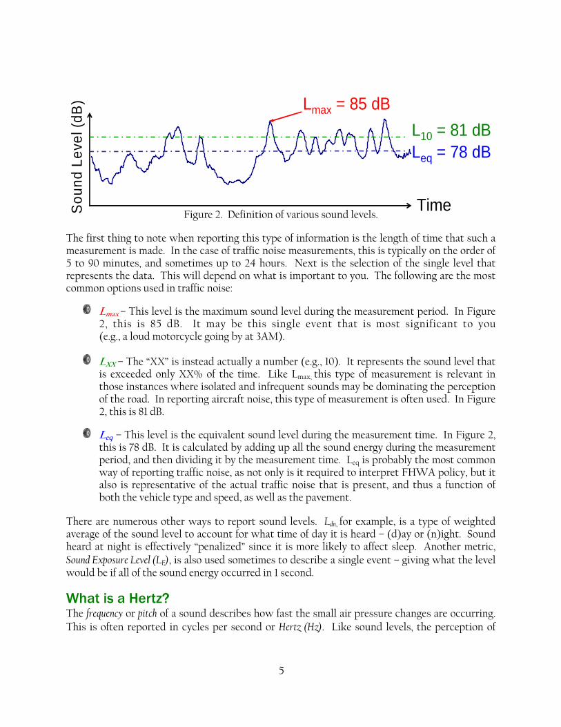
What is the difference between Lmax and Leq and L10 and…? In most situations, the sound levels around us will not stay the same from moment to moment. As someone talks, for example, we will experience higher levels as they speak, and lower levels when they stop. There are a number of ways to convert these types of non-uniform sounds into a single measurement (number). To illustrate how this can be done, Figure 2 shows what a sound level meter might produce if placed next to a road. It shows the rise and fall of the sound level over time. The sound from individual vehicles can be noted as they pass by the meter alongside the road. The levels of each vehicle vary depending on the type (e.g., car vs. a truck) and the distance between passing vehicles.
5
Lmax = 85 dB
TimeSou
nd L
evel
(dB
)
Leq = 78 dBL10 = 81 dB
Figure 2. Definition of various sound levels.
The first thing to note when reporting this type of information is the length of time that such a measurement is made. In the case of traffic noise measurements, this is typically on the order of 5 to 90 minutes, and sometimes up to 24 hours. Next is the selection of the single level that represents the data. This will depend on what is important to you. The following are the most common options used in traffic noise:
Lmax – This level is the maximum sound level during the measurement period. In Figure 2, this is 85 dB. It may be this single event that is most significant to you (e.g., a loud motorcycle going by at 3AM). LXX – The “XX” is instead actually a number (e.g., 10). It represents the sound level that is exceeded only XX% of the time. Like Lmax, this type of measurement is relevant in those instances where isolated and infrequent sounds may be dominating the perception of the road. In reporting aircraft noise, this type of measurement is often used. In Figure 2, this is 81 dB. Leq – This level is the equivalent sound level during the measurement time. In Figure 2, this is 78 dB. It is calculated by adding up all the sound energy during the measurement period, and then dividing it by the measurement time. Leq is probably the most common way of reporting traffic noise, as not only is it required to interpret FHWA policy, but it also is representative of the actual traffic noise that is present, and thus a function of both the vehicle type and speed, as well as the pavement.
There are numerous other ways to report sound levels. Ldn, for example, is a type of weighted average of the sound level to account for what time of day it is heard – (d)ay or (n)ight. Sound heard at night is effectively “penalized” since it is more likely to affect sleep. Another metric, Sound Exposure Level (LE), is also used sometimes to describe a single event – giving what the level would be if all of the sound energy occurred in 1 second.
What is a Hertz? The frequency or pitch of a sound describes how fast the small air pressure changes are occurring. This is often reported in cycles per second or Hertz (Hz). Like sound levels, the perception of
6
54
frequency is also non-linear. A change from 1000 Hz to 2000 Hz (an increase of 1000 Hz) is perceived in a similar way as a change from 2000 Hz to 4000 Hz (an increase of 2000 Hz). These doubling of frequencies are called octaves, and will be discussed in more detail later.
What frequencies matter? In addition to hearing over a wide range of sound levels, humans can also hear over a wide range of frequencies. Assuming you have no hearing loss, you may be able to hear sounds from 20 cycles per second (Hz) to 20,000 Hz. Human hearing is less sensitive near these extremes, and is often most sensitive in the range from 1000 to 4000 Hz. As we get older, or if our hearing has been damaged, we tend to lose our sensitivity to some frequencies, particularly those on the higher end of this range.
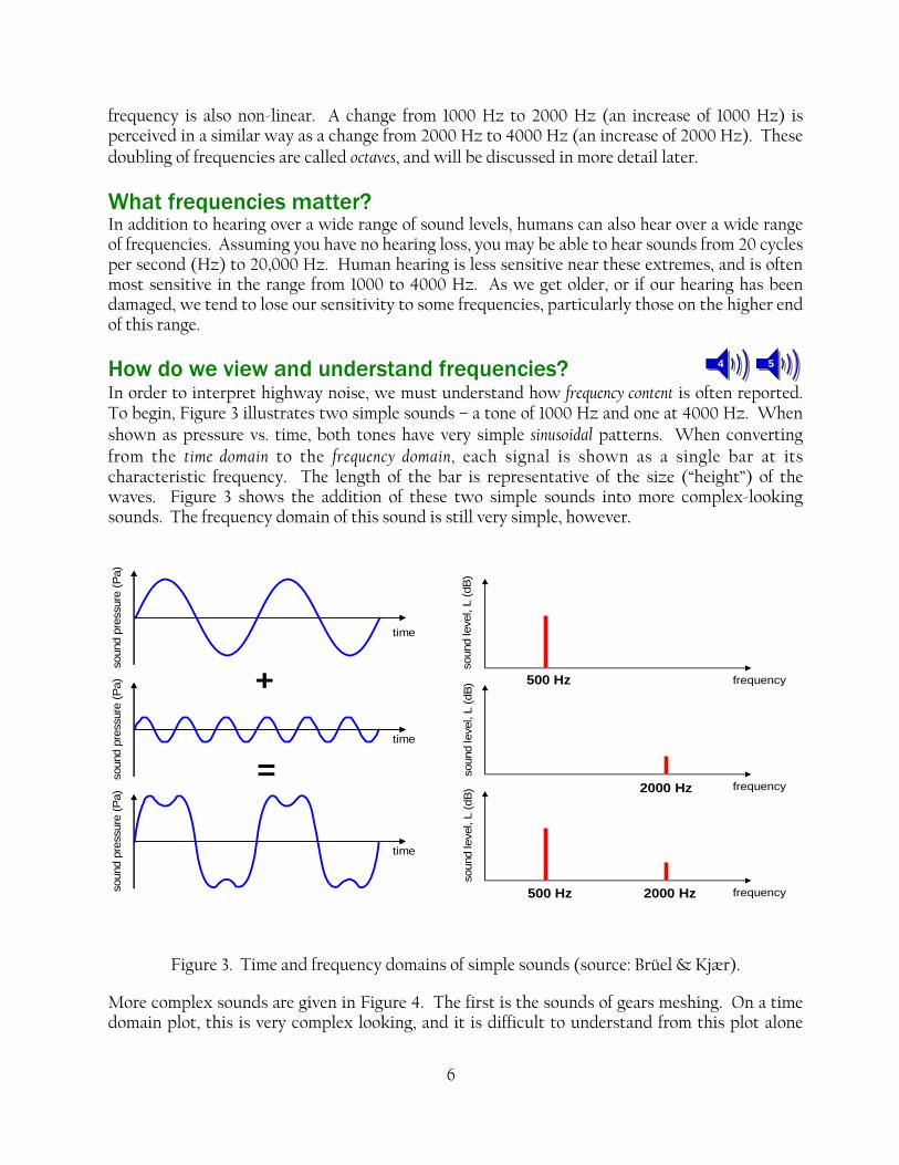
How do we view and understand frequencies? In order to interpret highway noise, we must understand how frequency content is often reported. To begin, Figure 3 illustrates two simple sounds – a tone of 1000 Hz and one at 4000 Hz. When shown as pressure vs. time, both tones have very simple sinusoidal patterns. When converting from the time domain to the frequency domain, each signal is shown as a single bar at its characteristic frequency. The length of the bar is representative of the size (“height”) of the waves. Figure 3 shows the addition of these two simple sounds into more complex-looking sounds. The frequency domain of this sound is still very simple, however.
Figure 3. Time and frequency domains of simple sounds (source: Brüel & Kjær).
More complex sounds are given in Figure 4. The first is the sounds of gears meshing. On a time domain plot, this is very complex looking, and it is difficult to understand from this plot alone
time
frequency
time
time
frequency
frequency
+
=
500 Hz
500 Hz
2000 Hz
2000 Hz
soun
d pr
essu
re (P
a)so
und
pres
sure
(Pa)
soun
d pr
essu
re (P
a)
soun
d le
vel,
L (d
B)so
und
leve
l, L
(dB)
soun
d le
vel,
L (d
B)

7
time
frequency
soun
d pr
essu
re (P
a)
soun
d le
vel,
L (d
B)time
frequency
soun
d pr
essu
re (P
a)
soun
d le
vel,
L (d
B)
time
frequency
soun
d pr
essu
re (P
a)
soun
d le
vel,
L (d
B)
what kind of sound this is. On the frequency domain plot, however, characteristic tonal peaks can be seen at various frequencies (likely corresponding to the number of teeth and speed of the gears). These peaks are sometimes an indication that a sound might be unpleasant. The second example looks similar to the first in the time domain, but very different in the frequency domain. As rain on the umbrella, this sound is more random (or broadband), and thus often more pleasant. The third sound is that of an anvil being hit. While very similar to the umbrella example in the frequency domain, it is much different in the time domain. This type of sound is transient, meaning that it changes significantly with time. This underscores the importance of looking at both the time and frequency domains when interpreting sounds.
Figure 4. Time and frequency domains of real sounds (source: Brüel & Kjær).
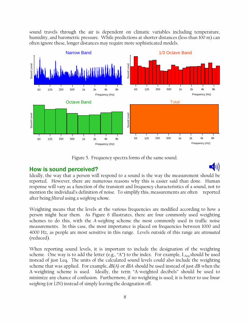
Figure 5 shows various ways that frequencies can be plotted for a sound. The first is called a narrow-band plot, and while very complicated looking, allows for subtle components of a sound to be identified. The second is a one-third-octave band plot that adds up the sound energy into various standardized bands. These bands simplify the reporting, but compromise some of the ability to interpret the sound. Octave bands can also be reported which sum the energy in groups of three consecutive third-octave bands. Each octave represents a doubling of frequency. Finally, a total level can be reported by summing all of sound energy in the octave bands together.
How does sound travel? Sounds can often be analyzed by breaking them down into a source, propagation path, and receiver. If the position and intensity of a source is known, along with the path, a good prediction can often be made of the sound level at the receiver. This calculation becomes increasingly complex, however, as things that may block or reflect sound are introduced. Furthermore, the way that
8
6
63 125 250 500 1k 2k 4k 8k
Soun
d Le
vel
Total
Frequency (Hz)63 125 250 500 1k 2k 4k 8k
Frequency (Hz)
Soun
d Le
vel
Octave Band
63 125 250 500 1k 2k 4k 8k
Frequency (Hz)
Soun
d Le
vel
1/3 Octave Band
Soun
d Le
vel
63 125 250 500 1k 2k 4k 8k
Frequency (Hz)
Narrow Band
sound travels through the air is dependent on climatic variables including temperature, humidity, and barometric pressure. While predictions at shorter distances (less than 100 m) can often ignore these, longer distances may require more sophisticated models.
Figure 5. Frequency spectra forms of the same sound.
How is sound perceived? Ideally, the way that a person will respond to a sound is the way the measurement should be reported. However, there are numerous reasons why this is easier said than done. Human response will vary as a function of the transient and frequency characteristics of a sound, not to mention the individual’s definition of noise. To simplify this, measurements are often reported after being filtered using a weighting scheme. Weighting means that the levels at the various frequencies are modified according to how a person might hear them. As Figure 6 illustrates, there are four commonly used weighting schemes to do this, with the A-weighting scheme the most commonly used in traffic noise measurements. In this case, the most importance is placed on frequencies between 1000 and 4000 Hz, as people are most sensitive in this range. Levels outside of this range are attenuated (reduced). When reporting sound levels, it is important to include the designation of the weighting scheme. One way is to add the letter (e.g., “A”) to the index. For example, LAeq should be used instead of just Leq. The units of the calculated sound levels could also include the weighting scheme that was applied. For example, dB(A) or dBA should be used instead of just dB when the A-weighting scheme is used. Ideally, the term “A-weighted decibels” should be used to minimize any chance of confusion. Furthermore, if no weighting is used, it is better to use linear weighting (or LIN) instead of simply leaving the designation off.

9
Figure 6. Weighting schemes for sound level calculation.
0
-20
-40
10 100 1k 10kSoun
d Pr
essu
re L
evel
Adj
ustm
ent
(dB
) AB
CD AB + C
D
Linear
Frequency(Hz)
-60
20k2k 5k200 50020 50
A-weighted – moderate sounds(most often used, but developed for < 55 dB)B-weighted – intense sounds (55-85 dB typ.)C-weighted – very loud sounds (>85 dB typ.)D-weighted – “noisiness” measure(sometimes used for aircraft noise)
10
Traffic Noise
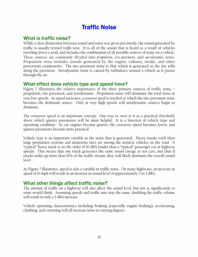
What is traffic noise? While a clear distinction between sound and noise was given previously, the sound generated by traffic is usually termed traffic noise. It is all of the sound that is heard as a result of vehicles traveling down a road, and includes the combination of all possible sources of noise on a vehicle. These sources are commonly divided into propulsion, tire-pavement, and aerodynamic noise. Propulsion noise includes sounds generated by the engine, exhaust, intake, and other powertrain components. The tire-pavement noise is that which is generated as the tire rolls along the pavement. Aerodynamic noise is caused by turbulence around a vehicle as it passes through the air.
What effect does vehicle type and speed have? Figure 7 illustrates the relative importance of the three primary sources of traffic noise – propulsion, tire-pavement, and aerodynamic. Propulsion noise will dominate the total noise at very low speeds. As speed increases, a crossover speed is reached at which the tire-pavement noise becomes the dominant source. Only at very high speeds will aerodynamic sources begin to dominate. The crossover speed is an important concept. One way to view it is as a practical threshold, above which quieter pavements will be most helpful. It is a function of vehicle type and operating condition. As car engines become quieter, the crossover speed becomes lower, and quieter pavements become more practical. Vehicle type is an important variable in the noise that is generated. Heavy trucks with their large propulsion systems and numerous tires are among the noisiest vehicles on the road. A “typical” heavy truck is on the order of 10 dBA louder than a “typical” passenger car at highway speeds. This means that one truck generates the same sound energy as ten cars, and thus if trucks make up more than 10% of the traffic stream, they will likely dominate the overall sound level. As Figure 7 illustrates, speed is also a variable in traffic noise. On many highways, an increase in speed of 10 mph will result in an increase in sound level of approximately 2 to 3 dBA.
What other things affect traffic noise? The amount of traffic on a highway will also affect the sound level, but not as significantly as some would think. Assuming speeds and traffic mix stay the same, doubling the traffic volume will result in only a 3 dBA increase. Vehicle operating characteristics including braking (especially engine braking), accelerating, climbing, and cornering will all increase noise to varying degrees.

11
7
Speed (mph)
Sound level (dBA)
65
75
70
60
80
15 30 60 7545
Overall Vehicle Noise
Tire-PavementNoise
PropulsionNoise
CrossoverSpeed
AerodynamicNoise
> 5035-50Trucks
20-3010-25Cars
AcceleratingCruisingVehicle
type
> 5035-50Trucks
20-3010-25Cars
AcceleratingCruisingVehicle
typeCrossover Speed (mph)
Figure 7. Speed effects on vehicle noise sources and crossover speed.
How can we control traffic noise? Within the FHWA policy found in 23 CFR 772, there are six possible methods to reduce traffic noise. If noise mitigation is found to be feasible and reasonable, noise barriers of some type are the most commonly used option. These often take the form of sound walls and/or earthen berms. The height of the barrier is a factor since if the line of sight between the source and the receiver is not broken, the barrier will not reduce the noise. Fortunately, most of the sound is generated close to the ground, which is the reason why most barriers can be effective to some degree. The effectiveness of a barrier is a function of how far away you are. For example, if you are directly behind a barrier, you may experience a decrease in sound level of typically 5 to 10 dBA. Once you are 100 to 150 m from the barrier, however, its effectiveness is different. A “shadow effect” will often occur, meaning that some of the traffic noise will “bend” around the top of the barrier. At this distance, however, background noise in the neighborhood may begin to dominate as spreading of the sound generated by the highway will decrease its level. It should be similarly noted that the effectiveness of a barrier can also be partially lost if there are any breaks in it – driveway access, for example.
12
8
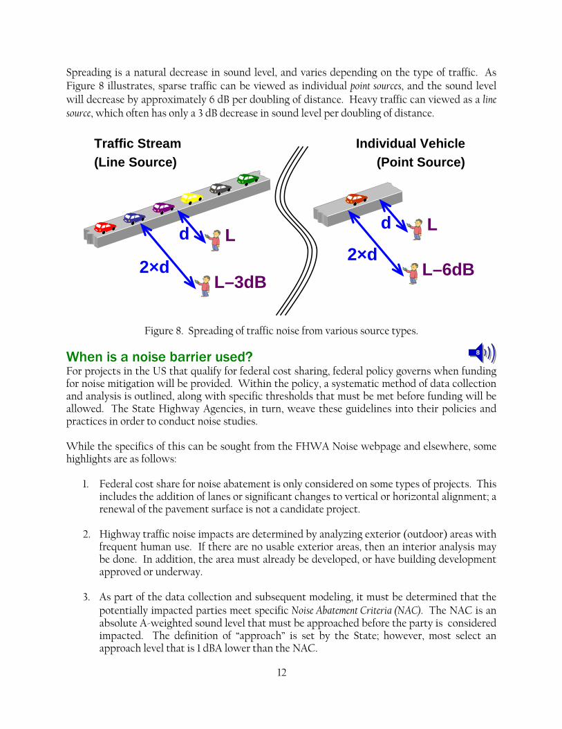
Spreading is a natural decrease in sound level, and varies depending on the type of traffic. As Figure 8 illustrates, sparse traffic can be viewed as individual point sources, and the sound level will decrease by approximately 6 dB per doubling of distance. Heavy traffic can viewed as a line source, which often has only a 3 dB decrease in sound level per doubling of distance.
Figure 8. Spreading of traffic noise from various source types.
When is a noise barrier used? For projects in the US that qualify for federal cost sharing, federal policy governs when funding for noise mitigation will be provided. Within the policy, a systematic method of data collection and analysis is outlined, along with specific thresholds that must be met before funding will be allowed. The State Highway Agencies, in turn, weave these guidelines into their policies and practices in order to conduct noise studies. While the specifics of this can be sought from the FHWA Noise webpage and elsewhere, some highlights are as follows:
1. Federal cost share for noise abatement is only considered on some types of projects. This includes the addition of lanes or significant changes to vertical or horizontal alignment; a renewal of the pavement surface is not a candidate project.
2. Highway traffic noise impacts are determined by analyzing exterior (outdoor) areas with
frequent human use. If there are no usable exterior areas, then an interior analysis may be done. In addition, the area must already be developed, or have building development approved or underway.
3. As part of the data collection and subsequent modeling, it must be determined that the
potentially impacted parties meet specific Noise Abatement Criteria (NAC). The NAC is an absolute A-weighted sound level that must be approached before the party is considered impacted. The definition of “approach” is set by the State; however, most select an approach level that is 1 dBA lower than the NAC.
d
2×d
L
L–3dB
d
2×dL
L–6dB
Traffic Stream(Line Source)
Individual Vehicle(Point Source)

13
4. The NAC is not intended to be a level that will be achieved after noise abatement is in
place. Furthermore, the NAC varies depending on the land use, and includes different criteria for different categories. Residential land falls under Category B, for example. In this case, an impact occurs when approaching 67 dBA. This level is about where conversational speech can be adversely affected. It is also far below a level that can lead to hearing damage, as Figure 1 illustrates.
5. The potential noise mitigation methods are then evaluated for being feasible and
reasonable in their ability to control noise. Only if these tests are passed can mitigation be approved for federal funding.
14
Sipes Tread Block Ribs Dimples Shoulder
Bead Bundle
Bead Filler
Body Piles
Carcass
Undertread
BeadAssembly
InnerLiner
Grooving
BeltsCap Piles
Bead Chafer
Sidewall
Edge Cover
Void Ratio
Tire-Pavement Noise
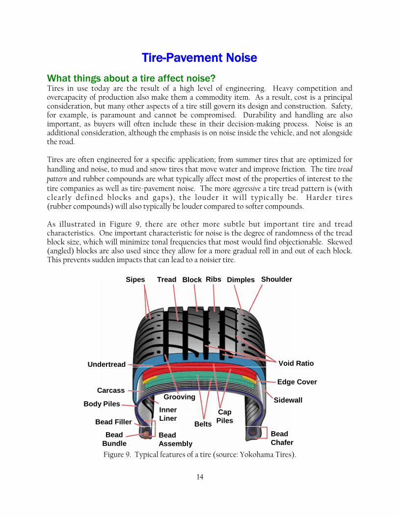
What things about a tire affect noise? Tires in use today are the result of a high level of engineering. Heavy competition and overcapacity of production also make them a commodity item. As a result, cost is a principal consideration, but many other aspects of a tire still govern its design and construction. Safety, for example, is paramount and cannot be compromised. Durability and handling are also important, as buyers will often include these in their decision-making process. Noise is an additional consideration, although the emphasis is on noise inside the vehicle, and not alongside the road. Tires are often engineered for a specific application; from summer tires that are optimized for handling and noise, to mud and snow tires that move water and improve friction. The tire tread pattern and rubber compounds are what typically affect most of the properties of interest to the tire companies as well as tire-pavement noise. The more aggressive a tire tread pattern is (with clearly defined blocks and gaps), the louder it will typically be. Harder tires (rubber compounds) will also typically be louder compared to softer compounds. As illustrated in Figure 9, there are other more subtle but important tire and tread characteristics. One important characteristic for noise is the degree of randomness of the tread block size, which will minimize tonal frequencies that most would find objectionable. Skewed (angled) blocks are also used since they allow for a more gradual roll in and out of each block. This prevents sudden impacts that can lead to a noisier tire.
Figure 9. Typical features of a tire (source: Yokohama Tires).

15
Air gaps in the tread pattern (including grooves and sipes) help to minimize some sounds from being generated, but also amplify other sounds. More on this later.
What things about a pavement affect noise? The influence of a pavement on tire-pavement noise is as equally important as the tire. Quieter pavements are typically smooth, but still provide adequate “ventilation”. To a lesser degree, pavements that are “softer” will also typically be quieter. Pavements, like tires, must not be built just for noise, however. Of paramount concern is safety, with additional considerations for cost and durability. Fortunately, we know that quieter pavements do not have to compromise these other characteristics of interest.
What makes tire-pavement noise? When the tire and pavement get together, they sure get noisy! And they do so in a very complex way. The sound often begins with various types of generation mechanisms. Making it complex is the fact that numerous mechanisms happen simultaneously, and to varying degrees, depending on the specific tire-pavement combination. Generation mechanisms are those that make sound. In the next section, we will discuss things that can amplify these sounds. To better understand the complexity of the various tire-pavement noise generation mechanisms, they are often described using physical analogies. The more prominent of these mechanisms are described as follows:
Tread impact (a.k.a. “The Hammer”) – As the tire rolls along the pavement, the tread on the tire and the texture on the pavement will come together as individual impacts. The resulting interaction can be seen as hundreds or even thousands of small hammer strokes occurring each second, each generating sound. See Figure 10.
Figure 10. “The Hammer” generation mechanism.
Radial vibrations
16
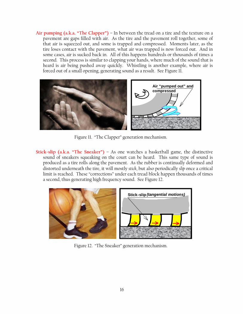
Air pumping (a.k.a. “The Clapper”) – In between the tread on a tire and the texture on a pavement are gaps filled with air. As the tire and the pavement roll together, some of that air is squeezed out, and some is trapped and compressed. Moments later, as the tire loses contact with the pavement, what air was trapped is now forced out. And in some cases, air is sucked back in. All of this happens hundreds or thousands of times a second. This process is similar to clapping your hands, where much of the sound that is heard is air being pushed away quickly. Whistling is another example, where air is forced out of a small opening, generating sound as a result. See Figure 11.
Figure 11. “The Clapper” generation mechanism.
Stick-slip (a.k.a. “The Sneaker”) – As one watches a basketball game, the distinctive
sound of sneakers squeaking on the court can be heard. This same type of sound is produced as a tire rolls along the pavement. As the rubber is continually deformed and distorted underneath the tire, it will mostly stick, but also periodically slip once a critical limit is reached. These “corrections” under each tread block happen thousands of times a second, thus generating high frequency sound. See Figure 12.
Figure 12. “The Sneaker” generation mechanism.
Air “pumped out” and compressed
Stick-slip (tangential motions)

17
Stick-snap (a.k.a. “The Suction Cup”) – A suction cup can stick to a smooth surface because of both adhesion and a vacuum that is created when the air in the cup is pushed out. As tread blocks interact with some pavements, a similar effect can occur, generating sound. See Figure 13.
Figure 13. “The Suction Cup” generation mechanism.
What makes tire-pavement noise even louder? The sound that is created by the various generation mechanisms is simply not enough to explain all of the noise that is heard. It is well accepted that a number of amplification mechanisms are also at play which increase the sound level. Amplification of tire-pavement noise is also complex. Like many musical instruments, the sound at some frequencies will be amplified more than others. As a result, if one seeks to reduce overall noise, they should target those frequencies that are amplified the most. To better understand specific amplification mechanisms that affect tire-pavement noise, physical analogies are again used. These include:
Acoustical Horn (a.k.a. “The Horn”) – The geometry of a tire and a pavement in contact includes a wedge-shaped segment of open air. Within this wedge, multiple reflections of sound generated near the throat can occur, much like the reflections that occur within a musical horn or megaphone. In the case of tire-pavement though, the horn is poor as it is open on two sides. The result is a significant amplification in the forward and aft direc-tions, along with a distortion of some frequencies. See Figure 14.
Figure 14. “The Horn” amplification mechanism.
Amplification effect by the horn
Adhesion “stick-snap”

18
Helmholtz Resonance (a.k.a. “The Pop Bottle”) – When you blow across the top of a pop bottle, a distinct tone can be heard. This occurs as the air in the neck of the bottle (acting as a mass) vibrates up and down on the pillow of air inside the bottle (acting as a spring). By itself, blowing creates very little sound. However, blowing across the bottle significantly amplifies the frequency that is distinct to that bottle. A similar geometry can be found close into the wedge where the tire and pavement meet. In this case, the mass and spring are side-by-side. The result is an amplification of some frequencies unique to the geometry of the tire and the pavement. See Figure 15.
Figure 15. “The Pop Bottle” amplification mechanism.
Pipe Resonance (a.k.a. “The Organ Pipe”) – When air is blown across an organ pipe, a
sound will be amplified that is unique to the length of the pipe and how many openings are in the pipe. On a tire, similar “pipe” geometries can be found as the various grooves and sipes on a tire are pinched off and opened up at various places underneath the contact patch. Sound that is generated elsewhere can be amplified within these pipes. See Figure 16.
Figure 16. “The Organ Pipe” amplification mechanism.
Air resonant radiation(Helmholtz resonance)
Pipe resonances in channelsformed in the tire footprint:Pipe resonances in channelsformed in the tire footprint:
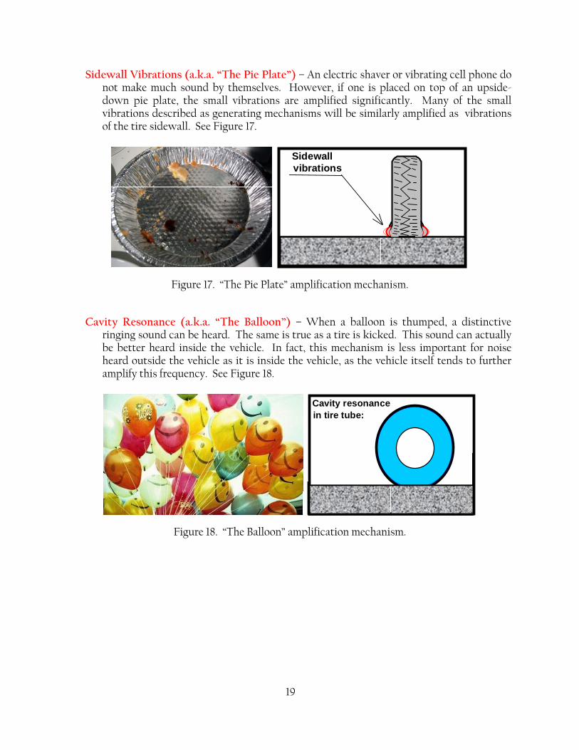
19
Sidewall Vibrations (a.k.a. “The Pie Plate”) – An electric shaver or vibrating cell phone do not make much sound by themselves. However, if one is placed on top of an upside-down pie plate, the small vibrations are amplified significantly. Many of the small vibrations described as generating mechanisms will be similarly amplified as vibrations of the tire sidewall. See Figure 17.
Figure 17. “The Pie Plate” amplification mechanism.
Cavity Resonance (a.k.a. “The Balloon”) – When a balloon is thumped, a distinctive
ringing sound can be heard. The same is true as a tire is kicked. This sound can actually be better heard inside the vehicle. In fact, this mechanism is less important for noise heard outside the vehicle as it is inside the vehicle, as the vehicle itself tends to further amplify this frequency. See Figure 18.
Figure 18. “The Balloon” amplification mechanism.
Sidewallvibrations
Cavity resonancein tire tube:
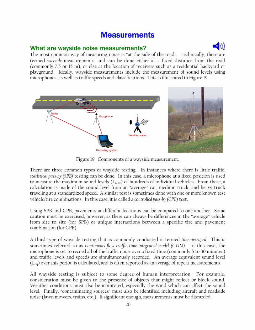
20
9
Measurements
What are wayside noise measurements? The most common way of measuring noise is “at the side of the road”. Technically, these are termed wayside measurements, and can be done either at a fixed distance from the road (commonly 7.5 or 15 m), or else at the location of receivers such as a residential backyard or playground. Ideally, wayside measurements include the measurement of sound levels using microphones, as well as traffic speeds and classifications. This is illustrated in Figure 19.
Figure 19. Components of a wayside measurement.
There are three common types of wayside testing. In instances where there is little traffic, statistical pass-by (SPB) testing can be done. In this case, a microphone at a fixed position is used to measure the maximum sound levels (Lmax) of hundreds of individual vehicles. From these, a calculation is made of the sound level from an “average” car, medium truck, and heavy truck traveling at a standardized speed. A similar test is sometimes done with one or more known test vehicle/tire combinations. In this case, it is called a controlled pass-by (CPB) test. Using SPB and CPB, pavements at different locations can be compared to one another. Some caution must be exercised, however, as there can always be differences in the “average” vehicle from site to site (for SPB) or unique interactions between a specific tire and pavement combination (for CPB). A third type of wayside testing that is commonly conducted is termed time-averaged. This is sometimes referred to as continuous flow traffic time-integrated model (CTIM). In this case, the microphone is set to record all of the traffic noise over a fixed time (commonly 5 to 30 minutes) and traffic levels and speeds are simultaneously recorded. An average equivalent sound level (Leq) over this period is calculated, and is often reported as an average of repeat measurements. All wayside testing is subject to some degree of human interpretation. For example, consideration must be given to the presence of objects that might reflect or block sound. Weather conditions must also be monitored, especially the wind which can affect the sound level. Finally, “contaminating sources” must also be identified including aircraft and roadside noise (lawn mowers, trains, etc.). If significant enough, measurements must be discarded.
RadarMicrophone
Recording system
Weather station

21
What are source noise measurements? A measure of tire-pavement noise as opposed to traffic noise is of increasing interest, particularly for those that wish to design and build quieter pavements. Source measurements measure sound “near the tire”. There are currently two principal techniques for measuring tire-pavement noise: close-proximity (CPX) and on-board sound intensity (OBSI). CPX is currently documented as a draft international (ISO) standard 11819-2. OBSI was initially developed by General Motors for use in tire evaluation at their test facilities. The technology was developed further by Dr. Paul Donavan of Illingworth & Rodkin as part of quiet pavement research for the Departments of Transportation in both California and Arizona. The OBSI measurement technique is now in the process of being standardized. As Figure 20 illustrates, both techniques are similar in that they include microphones positioned close to the tire-pavement contact patch. Both collect measurements as the vehicle is in motion. However, there are also some important differences:
The CPX method uses single microphones that measure sound pressure. OBSI uses
dual-microphone probes that measure sound intensity. The latter is directive, meaning that the measurements from each of the two microphones can be used to sort out the direction of the various sources.
Currently, the CPX and OBSI methods specify different positions for the microphone
including the height (from the ground), spacing between the front and rear positions, and distance from the tire sidewall. These differences mean that the generation and amplifying mechanisms will play different roles in the sound measured by the two tests.
While not required, CPX testing is often run in an enclosed trailer that is intended to
isolate the microphones from other sources of sound. Because of the ability of OBSI to identify the direction of a sound source, this is not required.
There is more experience with the OBSI method in the US, while the CPX technique has
been the preferred method elsewhere in the world. The measurements from any source measurement will be highly dependent on the tire that is used during testing. Specifications for both CPX and OBSI remain under development, with the identification of suitable test tires being a significant issue. Until recently, the vast majority of OBSI testing has been conducted using a Goodyear Aquatred III tire (P205/70R15). Recently, a newer Standard Reference Test Tire (SRTT) (P225/60R16) has been introduced and adopted for noise testing (ASTM F 2493). CPX testing in the US has also used the Aquatred, as well as a Uniroyal Tiger Paw AWP which differs only slightly from the new SRTT. According to the draft ISO CPX standard from 2000, the two most commonly used tires to date are an Avon/Cooper ZV1 (P185/65R15) and a Dunlop SP Arctic (P185/R14).
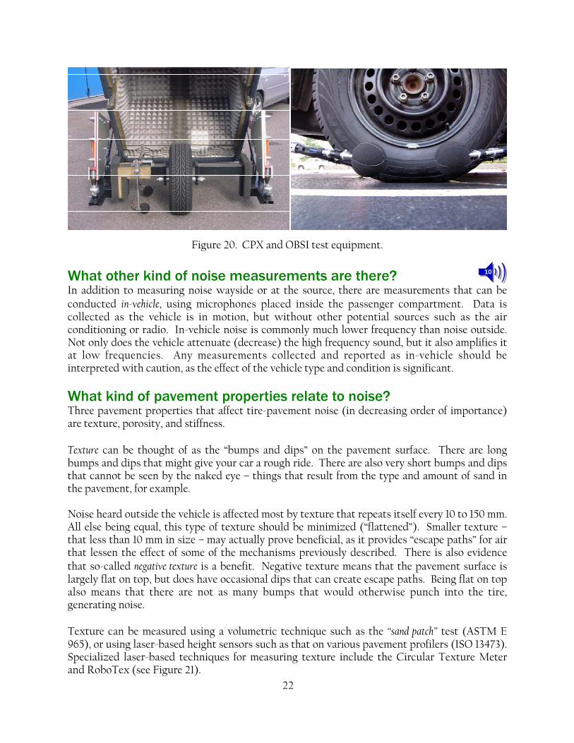
22
10
Figure 20. CPX and OBSI test equipment.
What other kind of noise measurements are there? In addition to measuring noise wayside or at the source, there are measurements that can be conducted in-vehicle, using microphones placed inside the passenger compartment. Data is collected as the vehicle is in motion, but without other potential sources such as the air conditioning or radio. In-vehicle noise is commonly much lower frequency than noise outside. Not only does the vehicle attenuate (decrease) the high frequency sound, but it also amplifies it at low frequencies. Any measurements collected and reported as in-vehicle should be interpreted with caution, as the effect of the vehicle type and condition is significant.
What kind of pavement properties relate to noise? Three pavement properties that affect tire-pavement noise (in decreasing order of importance) are texture, porosity, and stiffness. Texture can be thought of as the “bumps and dips” on the pavement surface. There are long bumps and dips that might give your car a rough ride. There are also very short bumps and dips that cannot be seen by the naked eye – things that result from the type and amount of sand in the pavement, for example. Noise heard outside the vehicle is affected most by texture that repeats itself every 10 to 150 mm. All else being equal, this type of texture should be minimized (“flattened”). Smaller texture – that less than 10 mm in size – may actually prove beneficial, as it provides “escape paths” for air that lessen the effect of some of the mechanisms previously described. There is also evidence that so-called negative texture is a benefit. Negative texture means that the pavement surface is largely flat on top, but does have occasional dips that can create escape paths. Being flat on top also means that there are not as many bumps that would otherwise punch into the tire, generating noise. Texture can be measured using a volumetric technique such as the “sand patch” test (ASTM E 965), or using laser-based height sensors such as that on various pavement profilers (ISO 13473). Specialized laser-based techniques for measuring texture include the Circular Texture Meter and RoboTex (see Figure 21).
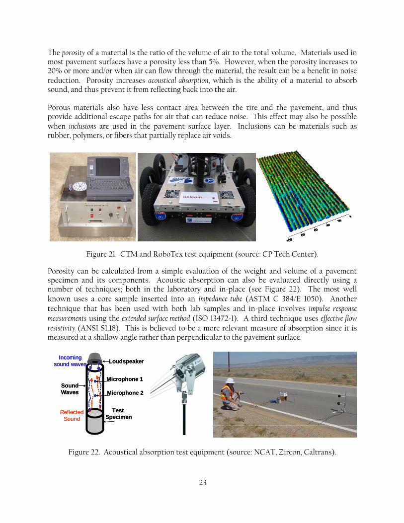
23
The porosity of a material is the ratio of the volume of air to the total volume. Materials used in most pavement surfaces have a porosity less than 5%. However, when the porosity increases to 20% or more and/or when air can flow through the material, the result can be a benefit in noise reduction. Porosity increases acoustical absorption, which is the ability of a material to absorb sound, and thus prevent it from reflecting back into the air. Porous materials also have less contact area between the tire and the pavement, and thus provide additional escape paths for air that can reduce noise. This effect may also be possible when inclusions are used in the pavement surface layer. Inclusions can be materials such as rubber, polymers, or fibers that partially replace air voids.
Figure 21. CTM and RoboTex test equipment (source: CP Tech Center).
Porosity can be calculated from a simple evaluation of the weight and volume of a pavement specimen and its components. Acoustic absorption can also be evaluated directly using a number of techniques; both in the laboratory and in-place (see Figure 22). The most well known uses a core sample inserted into an impedance tube (ASTM C 384/E 1050). Another technique that has been used with both lab samples and in-place involves impulse response measurements using the extended surface method (ISO 13472-1). A third technique uses effective flow resistivity (ANSI S1.18). This is believed to be a more relevant measure of absorption since it is measured at a shallow angle rather than perpendicular to the pavement surface.
Figure 22. Acoustical absorption test equipment (source: NCAT, Zircon, Caltrans).
Loudspeaker
Microphone 1
Microphone 2SoundWaves
Test Specimen
Incomingsound waves
ReflectedSound
Loudspeaker
Microphone 1
Microphone 2SoundWaves
Test Specimen
Incomingsound waves
ReflectedSound
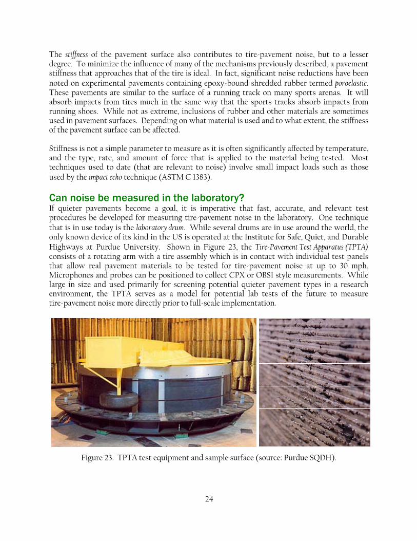
24
The stiffness of the pavement surface also contributes to tire-pavement noise, but to a lesser degree. To minimize the influence of many of the mechanisms previously described, a pavement stiffness that approaches that of the tire is ideal. In fact, significant noise reductions have been noted on experimental pavements containing epoxy-bound shredded rubber termed poroelastic. These pavements are similar to the surface of a running track on many sports arenas. It will absorb impacts from tires much in the same way that the sports tracks absorb impacts from running shoes. While not as extreme, inclusions of rubber and other materials are sometimes used in pavement surfaces. Depending on what material is used and to what extent, the stiffness of the pavement surface can be affected. Stiffness is not a simple parameter to measure as it is often significantly affected by temperature, and the type, rate, and amount of force that is applied to the material being tested. Most techniques used to date (that are relevant to noise) involve small impact loads such as those used by the impact echo technique (ASTM C 1383).
Can noise be measured in the laboratory? If quieter pavements become a goal, it is imperative that fast, accurate, and relevant test procedures be developed for measuring tire-pavement noise in the laboratory. One technique that is in use today is the laboratory drum. While several drums are in use around the world, the only known device of its kind in the US is operated at the Institute for Safe, Quiet, and Durable Highways at Purdue University. Shown in Figure 23, the Tire-Pavement Test Apparatus (TPTA) consists of a rotating arm with a tire assembly which is in contact with individual test panels that allow real pavement materials to be tested for tire-pavement noise at up to 30 mph. Microphones and probes can be positioned to collect CPX or OBSI style measurements. While large in size and used primarily for screening potential quieter pavement types in a research environment, the TPTA serves as a model for potential lab tests of the future to measure tire-pavement noise more directly prior to full-scale implementation.
Figure 23. TPTA test equipment and sample surface (source: Purdue SQDH).

25
11 12 13Quieter Pavements
What things make a quieter pavement? A quieter pavement can be designed and built in virtually any location subject to any environment and any amount and type of traffic. Furthermore, quieter pavements of both asphalt and concrete can achieve the same level of cost effectiveness, durability, and safety expected of our highways today. While much is still to be learned about quieter pavements, there is guidance that can be provided today to help us achieve this goal. To begin, we should recognize that quieter pavements are generally quieter for three reasons, in decreasing order of importance:
Texture – Goal: Keep it Small and Negative – Texture that will stab and poke at a tire will lead to undesired noise. As such, an objective common to all quieter pavements is to reduce the dimensions of any texture that is 10 mm or larger (“peak to peak”). However, some texture must remain to allow for “escape paths” for air. This remaining texture should be small (less than 5 mm) and negative (see Figure 24).
Figure 24. Conceptual schematics of “bad” and “good” texture.
Porosity – Goal: Make it High – Porosity can help absorb noise and reduce contact area, especially when in excess of 20%. However, since additional air voids can affect durability of any paving material, this tradeoff must be balanced. Inclusions (e.g., rubber, polymers, and fibers) in lieu of air voids continue to be looked at as a viable alternative. Stiffness – Goal: Keep it Low – While the most difficult to control for practical purposes, it is known that pavements that have stiffness characteristics approaching that of a tire can be quieter than those that are more typical of asphalt and concrete in
Bad
Good
1
3
2
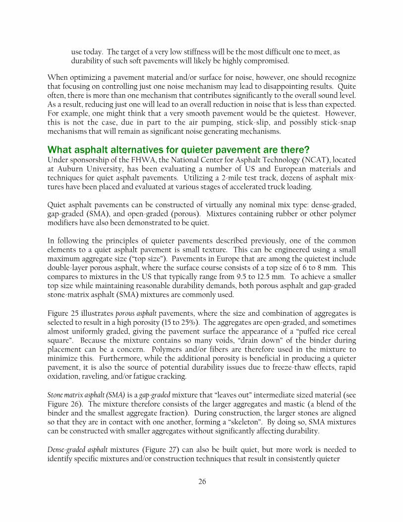
26
use today. The target of a very low stiffness will be the most difficult one to meet, as durability of such soft pavements will likely be highly compromised.
When optimizing a pavement material and/or surface for noise, however, one should recognize that focusing on controlling just one noise mechanism may lead to disappointing results. Quite often, there is more than one mechanism that contributes significantly to the overall sound level. As a result, reducing just one will lead to an overall reduction in noise that is less than expected. For example, one might think that a very smooth pavement would be the quietest. However, this is not the case, due in part to the air pumping, stick-slip, and possibly stick-snap mechanisms that will remain as significant noise generating mechanisms.
What asphalt alternatives for quieter pavement are there? Under sponsorship of the FHWA, the National Center for Asphalt Technology (NCAT), located at Auburn University, has been evaluating a number of US and European materials and techniques for quiet asphalt pavements. Utilizing a 2-mile test track, dozens of asphalt mix-tures have been placed and evaluated at various stages of accelerated truck loading. Quiet asphalt pavements can be constructed of virtually any nominal mix type: dense-graded, gap-graded (SMA), and open-graded (porous). Mixtures containing rubber or other polymer modifiers have also been demonstrated to be quiet. In following the principles of quieter pavements described previously, one of the common elements to a quiet asphalt pavement is small texture. This can be engineered using a small maximum aggregate size (“top size”). Pavements in Europe that are among the quietest include double-layer porous asphalt, where the surface course consists of a top size of 6 to 8 mm. This compares to mixtures in the US that typically range from 9.5 to 12.5 mm. To achieve a smaller top size while maintaining reasonable durability demands, both porous asphalt and gap-graded stone-matrix asphalt (SMA) mixtures are commonly used. Figure 25 illustrates porous asphalt pavements, where the size and combination of aggregates is selected to result in a high porosity (15 to 25%). The aggregates are open-graded, and sometimes almost uniformly graded, giving the pavement surface the appearance of a “puffed rice cereal square”. Because the mixture contains so many voids, “drain down” of the binder during placement can be a concern. Polymers and/or fibers are therefore used in the mixture to minimize this. Furthermore, while the additional porosity is beneficial in producing a quieter pavement, it is also the source of potential durability issues due to freeze-thaw effects, rapid oxidation, raveling, and/or fatigue cracking. Stone matrix asphalt (SMA) is a gap-graded mixture that “leaves out” intermediate sized material (see Figure 26). The mixture therefore consists of the larger aggregates and mastic (a blend of the binder and the smallest aggregate fraction). During construction, the larger stones are aligned so that they are in contact with one another, forming a “skeleton”. By doing so, SMA mixtures can be constructed with smaller aggregates without significantly affecting durability. Dense-graded asphalt mixtures (Figure 27) can also be built quiet, but more work is needed to identify specific mixtures and/or construction techniques that result in consistently quieter

27
pavements. The work at NCAT on these and other mixtures will result in more guidance in the near future.
The asphalt rubber friction course (ARFC) used in Arizona has received a lot of attention due to the large overlay initiative in the Phoenix metropolitan area. It is an open-graded material, but contains additional binder due to the addition of the rubber. Helping make ARFC a quieter
Figure 25. Porous asphalt schematic and photo.
Figure 26. Gap-graded SMA schematic and photo.
Figure 27. Dense-graded asphalt schematic and photo.
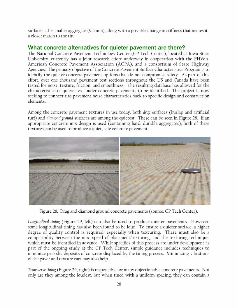
28
surface is the smaller aggregate (9.5 mm), along with a possible change in stiffness that makes it a closer match to the tire.
What concrete alternatives for quieter pavement are there? The National Concrete Pavement Technology Center (CP Tech Center), located at Iowa State University, currently has a joint research effort underway in cooperation with the FHWA, American Concrete Pavement Association (ACPA), and a consortium of State Highway Agencies. The primary objective of the Concrete Pavement Surface Characteristics Program is to identify the quieter concrete pavement options that do not compromise safety. As part of this effort, over one thousand pavement test sections throughout the US and Canada have been tested for noise, texture, friction, and smoothness. The resulting database has allowed for the characteristics of quieter vs. louder concrete pavements to be identified. The project is now seeking to connect tire-pavement noise characteristics back to specific design and construction elements. Among the concrete pavement textures in use today, both drag surfaces (burlap and artificial turf) and diamond ground surfaces are among the quietest. These can be seen in Figure 28. If an appropriate concrete mix design is used (containing hard, durable aggregates), both of these textures can be used to produce a quiet, safe concrete pavement.
Figure 28. Drag and diamond ground concrete pavements (source: CP Tech Center).
Longitudinal tining (Figure 29, left) can also be used to produce quieter pavements. However, some longitudinal tining has also been found to be loud. To ensure a quieter surface, a higher degree of quality control is required, especially when texturing. There must also be a compatibility between the mix, speed of placement/texturing, and the texturing technique, which must be identified in advance. While specifics of this process are under development as part of the ongoing study at the CP Tech Center, simple guidance includes techniques to minimize periodic deposits of concrete displaced by the tining process. Minimizing vibrations of the paver and texture cart may also help. Transverse tining (Figure 29, right) is responsible for many objectionable concrete pavements. Not only are they among the loudest, but when tined with a uniform spacing, they can contain a

29
“whine” that increases the annoyance even further. Quieter transverse tined pavements are possible, but are often found to have a short spacing between the tines – nominally 12 mm or less. Furthermore, randomizing this short spacing can minimize the potential for “whine”. Even with this nominal spacing, however, the potential remains for constructing an objectionable pavement in terms of noise. Both material compatibility and quality control issues must be addressed to help overcome this.
Figure 29. Longitudinal and transverse tined concrete pavements (source: CP Tech Center).
In Europe, a technique for concrete pavement surfacing termed exposed aggregate (Figure 30, left) is sometimes touted as a quiet concrete pavement. Measurements on similar surfaces placed in North America have not been favorable. Furthermore, noise measurements found in the literature show these pavements to be at a similar level to those constructed with more conventional concrete pavement textures that are typical in the US.
Figure 30. Exposed aggregate and porous concrete.
Finally, porous concrete pavements (Figure 30, right) have been built in trial sections. While many have measured quieter than any dense concrete, their durability remains an unresolved issue.
30
How do I choose a quieter pavement? Before any quieter pavement is selected, it is in the best interest of all stakeholders to evaluate a number of other criteria. These include the durability of the pavement; not only in resisting the effects of both traffic loads and climate, but also the ability of the pavement to remain quiet over time (acoustical durability). The cost of the pavement – both initially and over the life cycle – should also be evaluated and considered. Finally, safety must never be compromised. Any quieter pavement that is constructed should face the same scrutiny as any pavement for its ability to provide a safe stopping distance as well as other issues including vehicle handling and splash and spray. Tools for decision-making based on such different criteria are readily available. Some are based on the conversion of many of these factors to equivalent dollars, with further consideration to the time phasing of these costs by way of life-cycle costs. Other tools include multi-criteria analysis methods, which have historically been used in other industries where complex decisions must be made.

31
For More Information
Where can I read to learn more?
Tyre/Road Noise Reference Book by Ulf Sandberg and Jerzy Ejsmont www.informex.info Traffic Noise Model Technical Manual (FHWA-PD-96-010) An Introduction to Tire/Pavement Noise by Robert Bernhard, et al. (SQDH 2005-1) Advanced References Fundamentals of Acoustics by Lawrence E. Kinsler Signal, Sound, and Sensation by William M. Hartmann Noise and Vibration Control Engineering by Leo Beranek and István Vér
What are some good web sites?
Federal Highway Administration Noise - www.fhwa.dot.gov/environment/noise
Pavements - www.fhwa.dot.gov/pavement International Technology Scan on Quiet Pavement Systems in Europe - international.fhwa.dot.gov/quiet_pav
State Department of Transportation Arizona - www.quietroads.com California www.dot.ca.gov/hq/env/noise Washington - www.wsdot.wa.gov/Projects/QuieterPavement
Transportation Research Board Committees Noise and Vibration (ADC40) - www.adc40.org Surface Properties – Vehicle Interaction (AFD90) - www.trb.org/directory/comm_detail.asp?c=AFD90
Paving Industry Research Asphalt (NCAT) - www.ncat.us Concrete (National CP Tech Center) - www.cptechcenter.org
Institutes of Noise Control Engineering International - www.i-ince.org USA - www.inceusa.org
European Union Noise Policy - ec.europa.eu/environment/noise
Institute for Safe, Quiet, and Durable Highways (SQDH) - tools.ecn.purdue.edu/~sqdh
Center for Pavement Surface Characteristics - www.tcpsc.com

32
Who are we?
Robert Otto Rasmussen, Ph.D., P.E. (TX) Robert Otto Rasmussen is an internationally recognized expert in pavement engineering and construction, including the analysis and modeling of pavement smoothness, texture, and noise. He holds a B.S. in Civil Engineering from the University of Arizona, and a M.S.E. and Ph.D. from the University of Texas at Austin. He currently serves as Vice President and Chief Engineer of The Transtec Group, Inc., a pavement and materials engineering firm headquartered in Austin, Texas and is a registered professional engineer in the State of Texas. Dr. Rasmussen has authored dozens of peer-reviewed papers, and is an active member on numerous editorial boards, expert task groups, and industry groups including TRB, AAPT, ASCE, ACPA, RILEM, INCE, and ASA.
Robert J. Bernhard, Ph.D., P.E. (IN)
Robert J. Bernhard received a B.S. in Mechanical Engineering from Iowa State University in 1973, an M.S. in Mechanical Engineering from the University of Maryland at College Park in 1976, and his Ph.D. in Engineering Mechanics from Iowa State University in 1982. He joined Purdue University in 1982. He was the Director of the Ray W. Herrick Laboratories from 1994 through 2004, and has been the Director of the Institute for Safe, Quiet, and Durable Highways since 1998. He became the Associate Vice President for Research at Purdue University in December 2004. In 2007, Dr. Bernhard became Vice President for Research of Notre Dame University.
Ulf Sandberg, Sc.D.
Ulf Sandberg is a Senior Research Scientist at the Swedish National Road and Transport Research Institute in Linköping. He is also an Adjunct Professor at Chalmers University of Technology in Göteborg. He is known worldwide as one of the leading experts in tire-pavement noise, and is maybe most well known in the US as a co-author of the “Tyre/Road Noise Reference Book”. Dr. Sandberg’s accomplishments in this field are vast, and include service as chairperson and member on numerous ISO, TRB, and CEN committees related to highway noise.
Eric P. Mun
Eric P. Mun received his B.S. in Mechanical Engineering from The University of Texas at Austin in 2002. He joined The Transtec Group, Inc. in 2005 and is currently a Project Manager specializing in pavement surface characteristics. He has extensive experience in designing and building equipment systems for evaluating pavement surface characteristics and has collected and analyzed pavement noise, texture, and friction data on hundreds of pavement surfaces throughout North America.
Nicholas P. Miller, M.S.M.E. (Developer of accompanying Listening Experience)
Nicholas P. Miller is Senior Vice President of Harris Miller Miller & Hanson Inc. He started his work in environmental acoustics in 1970 at the University of North Dakota. In 1973, he began working at Bolt Beranek and Newman in highway noise and regulatory acoustics. He then helped to found Harris Miller Miller & Hanson in 1981. His recent innovations include revisions to sleep disturbance analysis and development of Virtual Soundscapes™ - a technique that permits listeners to hear how a place will sound.
14

33
What can I find in the listening experience? Introduction Is it Sound or Noise? Decibels Frequencies Complex Sounds The Perception of Sound Introduction to Traffic Noise Controlling Traffic Noise Controlled Pass-By Testing Comparing Noise Measurement Types Comparing Pavements at Wayside Comparing Pavements at the Source Pavement Variability Who are We?
1
5
4
3
2
14
13
12
11
10
9
8
7
6