CONCORDIA UNIVERSITY A GIS BASED MODELLING APPROACH …

CONCORDIA UNIVERSITY

A GIS BASED MODELLING APPROACH TO ASSESS LAKE

EUTROPHICATION

Linda El Farra

A Thesis

In

The Department

of

Building, Civil and Environmental Engineering

Presented in Partial Fulfillment of the Requirements

for the Degree of Master of Applied Science (Civil Engineering) at

Concordia University

Montreal, Quebec, Canada

April 2015

© Linda El Farra 2015

CONCORDIA UNIVERSITY

School of Graduate Studies

This is to certify that the thesis prepared

By: Linda El Farra

Entitled: A GIS BASED MODELLING APPROACH TO ASSESS LAKE

EUTROPHICATION

Submitted in partial fulfillment of the requirements for the degree of

Master of Applied Science (Civil Engineering)

Complies with the regulations of the University and meets the accepted standards with respect to

originality and quality.

Signed by the final examining committee:

Dr. M. Elektorowicz, _______________________ Chair

Dr. Z. Chen, BCEE, _______________________ Supervisor

Dr. A. Awasthi, CIISE, _______________________ External-to- Program

Dr. S. Rahaman, BCEE, _______________________ Examiner

Approved by

_________________________________

Chair of Department or Graduate Program Director

_________________________________

Dean of Faculty

Date 15/ 04 / 2014

iii

ABSTRACT

A GIS Based Modeling Approach to Assess Lake Eutrophication

Linda El Farra

Large proportion of the world’s readily available water supply is at risk due to the rapidly

increasing populations of certain types of harmful algae. During the photosynthesis, species like

blue-green algae and cyanobacteria consume nutrients and produce toxins that have potential

adverse effects to humans and animals.

This thesis focuses on developing a GIS-based statistical approach to explore the water

quality parameters facilitating the algae bloom, and to geographically map the extent and spread

of these parameters to enable tracking and prediction of potential algae outbreaks.

The relationship between Chlorophyll-a, which represents the concentration of algae

biomass, and the water quality parameters such as depth, phosphorus, nitrogen, alkalinity,

suspended solids, pH, temperature, electrical conductivity, dissolved oxygen and secchi depth is

analyzed though correlation matrix then by utilizing modeling techniques including multiple

linear, nonlinear regression, neural network and data mining prediction models are developed to

quantify the contribution from essential water quality parameters to eutrophication.

The developed GIS and statistical analysis approaches have been applied to the Lake

Champlain. The performance for the developed statistical, neural network and data mining

chlorophyll-a models has been examined through the comparison with the observed field data

and through statistical error analysis. Two new techniques have been examined in this thesis

study. First, data mining has helped to reveal the nonlinear behavior of algae growth in some

parts of the case study area. Second, the GIS spatial analysis is employed to visualize the spread

and extent of the water quality parameters and the algae chlorophyll-a, which graphically present

iv

the location-based impact of eutrophication on important lake water resources. For example, the

analysis of the GIS-based impact maps suggests that the algae is affecting the Vermont section of

Lake Champlain mainly the Northern and Southern section. The developed models suggest that

algae production is affected by nutrients particularly phosphorus. When phosphorus is

encountered at low to mild concentrations, the nutrient is linearly affecting algae production,

however, at extreme concentrations of the nutrient the relationship between nutrient and algae

production become nonlinear. The developed GIS model along with the statistical analysis

applied on lake Champlain suggest that Extreme levels of Nitrogen in north and Chloride in the

South caused deviations in the models prediction accuracy

v

ACKNOWLEDGEMENTS

I would like to thank my supervisor, Professor Dr. Zhi Chen, for his ongoing support

throughout this work and for offering me his helpful advice and guidance throughout all of my

studies at Concordia. Also I would like to express my sincere gratitude to Dr. Ann-Michele

Francoeur for her helping and support.

I am very grateful to Mr. Eric Smeltzer from “Vermont Department of Environmental

Conservation” who gave me insightful information on Lake Champlain.

I consider myself lucky to be surrounded by a supportive family and good friends. I

wouldn’t have been able to reach my goals without their encouragement and support.

vi

TABLE OF CONTENTS

LIST OF TABLES ....................................................................................................................ix

LIST OF FIGURES .....................................................................................................................x

LIST OF SYMBOLS..................................................................................................................xiii

LIST OF ABBREVIATIONS....................................................................................................xiv

CHAPTER 1: INTRODUCTION ................................................................................................1

1.1 Background …………………………...........................................................................2

1.2 Thesis Objective ............................................................................................................4

1.3 Organization of the Thesis ............................................................................................5

CHAPTER 2: LITERATURE REVIEW ……...........................................................................6

2.1 Lake Eutrophication …………………………………..................................................7

2.1.1 Phosphorus cycle.....…………………………………………………………7

2.1.2 Nitrogen cycle. …..………………………………………………….………8

2.2 Review of Lake Eutrophication Models. …………………………..…….…….……...9

2.3 GIS- Based Lake Assessment and Management…………………………...………...11

CHAPTER 3: METHODOLOGIES .........................................................................................12

3.1 Lake Nutrient Level Standards ...................................................................................13

3.2 Chlorophyll-a Lake Eutrophication Statistical Models that Use Multiple

Linear Regression (MLR) ..........................................................................................13

3.3 Chlorophyll-a Lake Eutrophication Models that Use Multiple Nonlinear

Regression (MNR) .....................................................................................................15

3.4 Chlorophyll-a Models that Use Data Mining (DM) ...................................................15

3.5 Chlorophyll-a Model Evaluation Techniques .............................................................16

3.5.1 Determination of coefficient R2 ...................................................................16

3.5.2 Standard error of the estimate ......................................................................17

3.5.3 Confidence interval and critical value .........................................................18

3.6 GIS Based Modeling and Assessment ........................................................................19

vii

CHAPTER 4 CASE STUDY: LAKE CHAMPLAIN EUTROPHICATION …....................22

4.1 An Overview of Lake Champlain ...............................................................................23

4.2 Raw Data and Variables for the Lake Champlain Case Study ...................................25

4.3 Lake Quality Criteria ..................................................................................................25

4.4 Data Collection and Quality Analysis .........................................................................30

A-Data source, format and units ..........................................................................30

B- Data quality analysis ........................................................................................30

C- Monitoring frequency ......................................................................................30

D-Gaps and range ................................................................................................33

4.5 Data Preparation .........................................................................................................35

A-Linear and nonlinear interpolation ...................................................................35

B-Extreme and outliers detection ...................................................................40

C-Selecting data range and variables ....................................................................43

4.6 Modeling Steps ...........................................................................................................44

4.6.1 Multiple linear regression ...........................................................................45

4.6.2 Neural network analysis ...............................................................................48

4.6.3 Data mining ..................................................................................................49

4.6.4 Geostatistical analysis ..................................................................................49

CHAPTER 5: LAKE CHAMPLAIN CHLOROPHYLL-a STATISTICAL

MODELING RESULTS .....................................................................................51

5.1 Correlation Matrix Analysis Results ...........................................................................52

5.2 Determination of Analysis Data Set ...........................................................................55

5.3 Chlorophyll-a Modeling Using Multiple Linear Regression (MLR) ..........................55

5.3.1 SPSS statistical analysis ...............................................................................55

5.3.2 ANOVA analysis of the variance of the MLR models ................................56

5.3.3 Multiple linear regression (MLR) results ....................................................56

5.3.4 Discussion of MLR model # 6 .....................................................................59

5.4 Lake Champlain Chlorophyll-a Modeling Using Multiple Nonlinear

Regression (MNR) .........................................................................................64

5.5 Lake Champlain Chlorophyll-a Modeling Using Neural Networks NN ....................64

viii

5.5.1 NN model #8 verification ...........................................................................69

5.6 Lake Champlain Chlorophyll-a Modeling Using Data Mining (DM) ........................71

5.6.1 DM modeling and water quality variables ...................................................71

5.6.2 Lake Champlain DM model #1 verification and comparison with

MLR model #6 and NN model #8 ...............................................................72

5.6.3 Comparison of chlorophyll-a DM, NN, MLR models with actual

observations .................................................................................................74

5.7 Discussion of the Results ............................................................................................78

5.7.1 Low to moderate water nutrient conditions .................................................78

5.7.2 High water nutrient conditions......................................................................78

5.7.3 Causes of the model errors ...........................................................................79

CHAPTER 6: LAKE CHAMPLAIN CHLOROPHYLL- a GIS SPATIAL ANALYSIS

RESULTS .............................................................................................................80

6.1 GIS Based Modeling Results ......................................................................................81

6.2 Determination of the Statistical Model Variables .......................................................81

6.3 Model Results and Model Configuration ....................................................................82

6.3.1 Statistical model with all input variables .....................................................82

6.3.2 Statistical model with selected variables .....................................................83

6.4 Spatial Trend Analysis ................................................................................................84

6.5 GIS Based Statistical Model Validation and GIS Results for TP and Chla ................92

CHAPTER 7 CONCLUSION AND CONTRIBUTION..........................................................96

7.1 Conclusion ..................................................................................................................97

7.2 Contributions of the Research .....................................................................................98

7.3 Future Studies ...........................................................................................................100

REFERENCES...........................................................................................................................102

APPENDICES............................................................................................................................114

Appendix A: Lake Champlain Outliers......................................................................................115

Appendix B: Multiple Linear Regression Matlab Code ............................................................117

Appendix C: Multiple Nonlinear Regressions ...........................................................................121

Appendix D: Data Mining Results .............................................................................................123

ix

LIST OF TABLES

Table 4.1 Names, abbreviations and definition of water quality monitoring parameters

(variables) used in the LEF modeling studies, using lake Champlain data.....................23

Table 4.2 Lake Champlain phosphorus criteria targets (2011) vs. observed values......................26

Table 4.3 Lake trophic criteria.......................................................................................................27

Table 4.4 Lake Champlain variables and their monitoring range and frequency .........................31

Table 4.5 Port Henry segment (07) of lake Champlain observed data………….….....................33

Table 4.6 Lake Champlain variables monitoring range and frequency ........................................43

Table 4.7 Lake Champlain yearly data for (1993-2011)................................................................46

Table 5.1 Pearson’s correlation matrix results …………..............................................................52

Table 5.2 Lake Champlain MLR modeling results for (2003-2011).............................................57

Table 5.3 Chlorophyll-a (Chla) MLR coefficients of the six lake Champlain MLR models……58

Table 5.4 ANOVA analysis of the six lake Champlain MLR models...........................................59

Table 5.5 Lake Champlain early years data, bootstrapping model results....................................63

Table 5.6 Results of lake Champlain DM model #1for (1992-2011)............................................71

Table 5.7 Summary of chlorophyll-a models described in this thesis. .........................................78

Table 6.1 GIS based model #1(OLS) results. ……………...........................................................82

Table 6.2 GIS based model #2 (OLS) results……........................................................................83

x

LIST OF FIGURES

Figure 2.1 Phosphorus cycle in lake Champlain……………………………………..………..…..7

Figure 2.2 Nitrogen cycle in lake Champlain. …………………………………………..………..9

Figure 3.1 R2 for unfit models ......................................................................................................17

Figure 3.2 Error distributions.........................................................................................................18

Figure 3.3 Bell shape error distribution ........................................................................................18

Figure 3.4 GIS hierarchy ...............................................................................................................20

Figure 3.5 Lake Champlain eutrophication modeling using the GIS ...……………….…...........21

Figure 4.1 Lake Champlain watershed .........................................................................................24

Figure 4.2 Phosphorus levels in Lake Champlain and water quality criteria ...............................29

Figure 4.3 Lake Champlain monitoring stations............................................................................32

Figure 4.4 Nonlinear curve types ..................................................................................................34

Figure 4.5 Yearly calcium data for lake Champlain station 02.....................................................35

Figure 4.6 The Mann–Kendall test and the interpolation ………………….................................36

Figure 4.7 Yearly TP, Cl and minerals chart for lake Champlain Port Henry...............................37

Figure 4.8 Data mining (FindGraph) analysis …..........................................................................38

Figure 4.9 Data mining (FindGraph) results..................................................................................39

Figure 4.10 Minerals Fourier prediction for station 02 ...............................................................39

Figure 4.11 Screening Outlier daily data of TP for station 02......................................................42

Figure 4.12 Model flowchart verification……….……………….................................................45

Figure 4.13 Neuron in a neural network ......................................................................................48

Figure 4.14 Lake Champlain polygon creation………..................................................................50

Figure 5.1 Cross correlation scatter plots for 8 independent water quality variables and the

dependent variable chlorophyll-a…………………………………...…………...........53

Figure 5.2 MLR model #6 standard error distribution...................................................................60

Figure 5.3 Lake Champlain chlorophyll-a levels by years (2003-2011) with MLR.....................61

Figure 5.4 Lake Champlain chlorophyll-a levels by years (1992-2002) with MLR.....................62

Figure 5.5 NN analysis water quality variables importance chart (top panel) and Chla observed

values vs. NN model #8 predicted values for Chla (bottom panel)……………...…...66

Figure 5.6 NN synaptic weight chart for lake Champlain later years data (2003-2011)…...........67

Figure 5.7 Lake Champlain chlorophyll-a levels by years (2003-2011) with NN........................68

xi

Figure 5.8 Lake Champlain chlorophyll-a levels by years (1992-2002) with NN........................70

Figure 5.9 Observed lake Champlain monitoring data (1992-2003) compared to predictions

generated by three chlorophyll a models..………………………………...…….…….73

Figure 5.10 Observed lake Champlain monitoring data (2012 and 2013) compared to predictions

from MLR model. ……………………………..…....................................................75


from NN model. …………..…………………………...............................................76


from DM model..……………………………………………………........................77

Figure 6.1 GIS-ordinary least squares analysis……......................................................................82

Figure 6.2 GIS Kriging inputs …..................................................................................................85

Figure 6.3 GIS map showing a summary of lake Champlain total phosphorus levels………..…87

Figure 6.4 GIS map showing a summary of lake Champlain total nitrogen (TN) levels …….....88

Figure 6.5 GIS map showing a summary of lake Champlain chloride (Cl) levels .......................89

Figure 6.6 GIS map showing a summary of lake Champlain secchi depths .................................90

Figure 6.7 GIS map showing a summary of lake Champlain alkalinity levels .............................91

Figure 6.8 GIS maps comparing lake Champlain chlorophyll-a observed levels with TP observed

levels between (2004-2011)……………………………………………..…............... 93

Figure 6.9 Lake Champlain water quality monitoring station observed chlorophyll-a levels

compared to GIS model# 2 predicted levels.................................................................94

Figure 6.10 Lake Champlain monitoring station observed Chlorophyll-a levels vs. MLR model#6

predicted levels……..…………………………………………………..……....…...95

xii

LIST OF SYMBOLS

RegAlk Alkalinity

Adjusted coefficient of determination

ANOVA Analysis of the variance

Chl-a Chlorophyll-a (μg/L)

Cl Chloride (μg/L)

R2 Coefficient of determination

β Coefficient of lake variables

CI Confidence interval thresholds

CABs Cynobacteria algal blooms

DM Data mining

DO Dissolved oxygen (μg/L)

DIC Dissolve inorganic carbon (μg/L)

DOC Dissolve organic carbon (μg/L)

ε Error

T Iron (μg/L)

TKN Kjldahl nitrogen (μg/L)

TPb Lead (μg/L)

Y Model output (Dependent variable)

Z Model Inputs (independent variables)

TK Potassium (μg/L)

Ŷ Predicted value

Secchi Secchi depth (m)

TNa Sodium (μg/L)

TN Total ammonia (μg/L)

xiii

TempC Temperature (deg C)

TCa Total calcium (μg/L)

TMg Total magnesium (μg/L)

TMDLs Total maximum daily loads

TNOX Total nitrate nitrate (μg/L)

TN Total nitrogen (μg/L)

TP Total phosphorus (μg/L)

TOC Total organic carbon (μg/L)

TSS Total suspended solids

xiv

LIST OF ABBREVIATIONS

DEC Department of environmental conservation

EBK Empirical Bayesian Kriging

ESRI Environmental systems research institute

EPA Environmental protection agency

GIS Geographic information system

GWR Geographically weighted regression

IWRM Integrated water resource management

IDW Inverse distance weighted

MLR Multiple linear regression

MNR Multiple non linear regression

MK Mann–Kendall test

NN Neural network

OLS Ordinary least square

SR Symbolic Regression

TSI Trophic state index

WHO World health organization

THMs Trihalomethanes

USGS US Geological survey

VIF Variance inflation factor

1

CHAPTER 1

INTRODUCTION

2

INTRODUCTION

Water bodies respond differently to increased amounts of nutrients (Correll, 1998). Many

factors contribute to eutrophication, including: hydrologic conditions, ecosystems, geology

(Correll, 1998), sediment loading capacity (Froelich, 1988), and both urban and agricultural land

use (Short et al., 1996).

1.1 Background

The 2014 US Geological survey (USGS) report indicated that of the 1.386 of total

water on earth, only 0.77% (10.7 ) is usable fresh water and 1.74% is unusable fresh water

present in ice caps, frozen glaciers and permanent snow. Unfortunately, a large proportion (70%)

of the world’s usable water supply is at risk due to contamination by environmentally harmful

Cyanobacteria (also called blue-green algae). Cyanobacteria range in colour from green to red,

and form large masses (called algal blooms) in warm shallow water that is slow moving or still.

During photosynthesis, cyanobacteria blooms consume nutrients essential for lake biome

survival and produce toxins that are poisonous to the humans and wildlife living in the lake

environment. These toxins include neurotoxins (affect the nervous system), and hepatotoxins

(affect the liver), as well as those that irritate the skin and eyes.

The microcystins are a group of approximately 50 toxins produced by the

cyanobacterium microcystis aeruginosa. These are important because they are chemically

extremely stable in water of widely varying temperature and pH. Microcystin-LR is the most

widely studied because it is found in fresh water supplies worldwide, and is undetectable by odor,

taste or appearance. Symptoms of microcystin poisoning include diarrhea, abdominal pain,

nausea, vomiting, headache, fever, irritated eyes and skin, and allergic reactions. Unfortunately,

boiling microcystin-contaminated water does not remove the toxins or destroy their activity.

Chlorophyll-a (also called chlorophyll a) is a plant pigment that is a primary electron

donor in the electron transport chain and essential for photosynthesis. Chlorophyll-a can be used

as a biomarker for the presence of cyanobacteria, as there is a direct relationship between the

mass of the cyanobacterial algal bloom and the concentration of chlorophyll-a in fresh water.

3

These include the following physicochemical parameters of water: 1) temperature; 2) pH;

3) electrical conductivity; 4)-6) concentration of phosphorus, nitrogen, and dissolved oxygen; 7)

secchi depth (a measure of water clarity, inversely proportional to CAB growth). Secchi depth is

measured using a circular secchi disk lowered into the water until it is not visible. Suspended

solids, including CABs reduce water clarity.

Eutrophication is the oversupply of artificial or natural substances, mainly phosphates

(e.g. pollution from fertilizers, sewage and detergents) to an aquatic system, which promotes the

excessive growth and decay of plants and bacteria, including algal blooms. After these organisms

die, oxygen depletion (hypoxia) occurs, which then inhibits the growth of fish and other

organisms in the environment. Eutrophication decreases the value of lakes and rivers and impairs

drinking water treatment. Eutrophication is one of most significant and widespread water quality

concerns in the global environment. It causes premature ageing of lakes and other water bodies.

The estimated damage cost of cultural eutrophication (from human activities) in the U.S alone

exceeds $2.2 billion annually (Dodds et al., 2009). The ability of a lake to recover from

eutrophication depends on the quantity of phosphorus in the lake sediment and in the volume of

water in contact with the sediment. It may take decades before nutrients are naturally flushed out

of lakes (Chambers et al., 2001; Hiscock et al., 2003).

Several studies have been published around lake Champlain, for example in 1989 a group

of scientists from the Vermont Department of Environmental Conservation published a

comprehensive study on lake Champlain, and concluded that it would be unrealistic to use daily

data for lake Champlain to detect emerging lake eutrophication problems (Smeltzer et al., 1989),

then in 1997 satellite images for the watershed was used to estimate the proportions of the

baseline nonpoint source loads attributed (Millette, 1997), and in 2009 a Danish study suggested

that eutrophication in lake Champlain is affected by the climate changes (Jeppesen ,2009). Many

other studies around eutrophication are found and reviewed in section 2.2 and 2.3, and only a handful

of these studies dealt with the GIS location characterization of water bodies (Aaby, 2005), and

barely few studies exist that used data mining and computing power to reveal hidden pattern and

information within the waterbodies data different timeframes (Petersen et al., 2001; Chen et al.,

2003 and Chau et al., 2007).

This study presents a new approach for exploding algae and eutrophication models

by searching for linear and nonlinear models using data mining, neural network and multiple

4

linear regression model throughout the different lake data timeframes, and by utilizing GIS

location information to investigate the location impact on the lake eutrophication and algae

spread.

1.2 Thesis Objective

Few large-scale watershed eutrophication studies have been reported, and these have

primarily focused on marine and coastal waters rather than on fresh water lakes, streams, rivers

and reservoirs (Arheimer et al., 2000; Nixon et al., 2002). Objectives of this thesis study

include:

A. To quantify the environmental variables associated with lake water quality such as: depth,

phosphorus, nitrogen, alkalinity, suspended solids, pH, temperature, electrical

conductivity, dissolved oxygen concentration and secchi depth contributions to algae

bloom.

B. To develop new statistical and generic algorithm based water quality models including

data mining, nonlinear regression, and neural networks to assess and help to manage lake

eutrophication

C. To couple the developed lake eutrophication models with geographical information

systems (GIS) to examine the location importance and impact on algae spread.

D. To apply the developed methodology to the lake Champlain to further develop and

validate field scale statistical linear and nonlinear chlorophyll-a models using data mining,

neural network and multiple regression modeling techniques.

5

1.3 Organization of the Thesis

This thesis is organized in the following seven chapters

Chapter 1 defines the scope of the thesis, and introduces eutrophication and its impact

on cyanobacterial algal bloom (CABs). Chapter 2 presents reviews of related literatures on

eutrophication statistical studies, data mining and GIS-based studies on eutrophication. Chapter

3 summarizes the analyses used to create the chlorophyll-a models and the techniques used to

evaluate the models. Chapter 4 presents the Lake Champlain case study data and discusses the

methods used to prepare the raw data for the analysis. In Chapter 5 data for the water quality

parameters that contribute to CAB are analyzed using various techniques, the analyses are

verified, and the results are compared to find the optimal set of prediction models. Chapter 6

shows how ArcGIS was incorporated to generate maps that illustrate the extent and spread of the

CABs. Finally, Chapter 7 summarizes the results and provides suggestions and recommendations

for future research.

6

CHAPTER 2

LITERATURE REVIEW

7

2.1 Lake Eutrophication

Eutrophication is the process where a waterbody progresses from its current state to its

extinction by gradual accumulation of nutrients and organic biomass (Das, 2003). Nutrients

generally enter aquatic ecosystems sorbed to soil particles that are eroded into lakes, streams, and

rivers (Sharpley et al., 1994). Human activities, excess use of fertilizers, mining phosphorus,

animal feeds, agricultural crops, and other products, causing excess amount of nutrients to

accumulate in soil thus altering the global phosphorus cycle (Schindler, 1977). The increasing

nutrients levels in the soil elevate the potential amount that carried by runoff water to the aquatic

ecosystems (Fluck et al., 1992).

2.1.1 Phosphorus cycle

Usually external loading is the main factor determining the lake’s trophic status because

of its large scale (Horne 1998); In 2005 a study published by the European Environmental

Agency (EEA) suggested that: although phosphorus and nitrate concentrations in inland

freshwater systems declined, eutrophication continued and haven’t stopped, the continuation of

the eutrophication was due to internal loading, therefore nutrients released to the water column

from the sediment is a factor to be considered in lake eutrophication (Bostrom et al., 1988) and

(Elwood et al., 1983).

Figure 2.1 Phosphorus cycle in lake Champlain. Source: http://prezi.com

accessed on August 2014

8

Internal and external loading of phosphorus into a lake body is referred to as phosphorus

cycle, and this loading is the results of phosphorus being very biologically active elements.

Figure 2.1 shows the phosphorus cycle in Lake Champlain, where phosphorus arrives into the

lake though runoff water or sorbed through soil particles. The phosphorus compounds are then

hydrolyzed either chemically or enzymatically to orthophosphate which is the only form of

phosphorus that can be digested by algae or microbial (Smith et al., 2009). Excess and heavy

particulates of phosphorus are deposited to the bottom and gradually form the sediment part of

sediment phosphorus is released back into the water column as orthophosphate or it stays in the

sediment and forms phosphate rock formation, which later on is dissolved by rain, snowmelt,

irrigation or runoff water and is deposited back into the soil, rivers and lakes to eventually makes

sediments rock formation (Goodwin, 2011).

2.1.2 Nitrogen cycle

When 71% of the earth surface is water, and 80% of the atmosphere is Nitrogen gas

N2 ,and when it takes millions of years for the rock sediment carrying phosphorus to raise up to

the surface then moved by runoff water or sorbed through soil particle for the phosphorus to

complete its cycle, while it may only takes days or even less for the nitrogen to complete its

cycle, then it becomes clear why nitrogen concentration is 16 times higher phosphorus in open

waters (Rydin and Rast, 1992).

Nitrogen exists in many forms, one of its form is ammonia NH3; Ammonia comes from

plant, animal wastes, decomposition of organic nitrogen and is used extensively in fermentation

(Luvalle et al., 1999) and as a cleaning agents; Ammonia has a deadly effect on fish and plant

and it encourages algae growth.

9

Figure 2.2 Nitrogen cycle in lake Champlain; Source: http://image.frompo.com/w/peerless-travels

accessed on August 2014

2.2 Review of Lake Eutrophication Models

The German agricultural chemist Justus von Liebig conducted the first eutrophication

study in 1950. Prior to this, Weber (1907) and Johnstone (1908) found a link between nutrients

and aquatic productivity (reviewed in Smith et.al, 1999). In the years that followed several

eutrophication studies were conducted; the majority of those studies focused on statistical

analytical techniques.

Due to the widespread of the eutrophication problems in fresh water supplies, many

studies were made in attempt to find the cause and solution, and in this section I presented the

different unique approaches I found related to topic, however it is worth to mention that the

sequence of studies is not necessary in a historical essay.

In 1973, Dieter Imboden developed a phosphorus model for Lake Lucerne eutrophication

using oxygen consumption as a function of phosphorus loading. Dieter’s model calculates the

mean Oxygen O2 consumption in water as a function of phosphorus loading and gives the critical

P-loading values above which the lake turns eutrophic for changing mean depth of the Lake and

hydraulic loading factor. The model produces a general rough behavior for lakes categorization

by elements and was not able to explain the cause behind the CABs in the lake. Another different

approach to instigate lake eutrophication was made by Lotter, who used the annual layer of

10

sediment in rocks (varve) to model the historical eutrophication of Lake Baldeggersee in

(Switzerland), and although eutrophication is suggested to be highly correlated with sediment

(Lijklema, 1980), however Lotter’s climate and trophic state models were only able to justify one

third of the variance data. (Lotter et al., 1997).

Many of the analytical eutrophication studies simplify the complexity between the lake

variables and eutrophication, and use multiple linear regression MLR which is technique that

attempts to find the relationship between several explanatory variables and a response variable

by fitting a linear equation to the training data. (Cüneyt, 1999; Xia et al., 2011), while other

eutrophication studies use more complex technique such as fuzzy logic to study eutrophication

(Selçuk et al., 2004).

In recent years with the availability of computing power there was a growing tendency to

use neural network to create eutrophication models (Recknagel et al., 1997). Some of those

studies used artificial neural networks (Yabunaka et al., 1997; Scardi et al., 1999; Jeong et al.,

2001 and Xia et al., 2011), while other used fuzzy and neuro-fuzzy techniques (Maier et al.,

2001); and most recently with the advances in software development, DM techniques started to

show in eutrophication studies (Petersen et al., 2001; Chen et al., 2003).

Although many advances were made, the wide variation in water body scenarios (e.g.

naturally occurring seasonal and annual variations in water quality parameters), and the

complexity between nutrients and eutrophication in a dynamic ecosystem made it a challenge to

develop a defined standard that defines water eutrophication (Correll, 1998). Different studies

provided distinctive eutrophication model.

In summary, the literature review showed:

1) There are many different analysis methods available to predict freshwater lake eutrophication

and CABs mass growth.

2) Several models are required to accurately deal with all lake scenarios (low vs. high nutrient

concentrations).

3) The most important predictive parameters for lake eutrophication and CABs mass growth

were total nitrogen (TN) and total phosphorus (TP) in the water.

4) Most studies focused on solving the eutrophication problem using standard analysis

techniques that do not address the nonlinearly problem of lake eutrophication at extreme

concentrations.

11

5) None of the studies utilized data mining techniques to model eutrophication problem in the

lakes, and there is a lack of comprehensive research to formalize the relation between water

variables and algae bloom.

2.3 GIS- Based Lake Assessment and Management

In 1973, ESRI developed the first commercial GIS system, the Maryland Automated

Geographic Information System (ESRI, 2006). They subsequently developed individual tools

(e.g. ArcInfo workstation, ArcView GIS 3.x, MapObjects, ArcSDE), which were integrated as

ArcGIS in 1999. Hiscock and coworkers utilized GIS to study phosphorus loading with land use,

soil type and rainfall in the Florida basins (Hiscock et al., 2003). Their results indicated that the

amount of developed land and the phosphorus loading have a strong correlation with lake

eutrophication.

In 2008, Dirk Craigie suggested using GIS as a resource to incorporate geographically

linked data used in the Integrated Water Resource Management (IWRM) system (Dirk, 2008).

Hameed’s group used GIS analysis to classify 50 inland lakes in Sweden according to their

degree of eutrophication and acidity, based on water pH and/or alkalinity monitoring data

(Hameed, 2010).

In 2011 Gupta used GIS to evaluate nitrogen and phosphorus levels in the Rönneå River

drainage basin in Sweden, and to estimate future discharge into the basin (Gupta et al., 2011).

Akdeniz used the inverse distance weighted (IDW) method of ArcGIS to create trophic state

index (TSI) maps for the shallow Uluabat Lake in Turkey (Akdeniz et al., 2011). Anoh used GIS

to study eutrophication in the Taabo River (Ivory Coast) using multi criteria analysis of water

quality parameters, which highlighted the areas in the watershed that required protection (Anoh

et al., 2012). Lake Michigan was studied using satellite images from MODIS to predict

chlorophyll-a concentration, the results showed the possibility of using satellite images

effectively to track algae (Huang, Deng, 2013).

In conclusion, GIS provides a powerful method to analyze lake eutrophication and the

growth of cyanobacteria algal blooms (CABs) spatially and to help effectively manage large-

scale lake eutrophication in countries worldwide.

12

CHAPTER 3

METHODOLOGIES

13

3.1 Lake Nutrient Level Standards

There is currently no world standard for acceptable nutrient levels in lakes, because each

presents a unique ecosystem, which is highly variable due to natural seasonal variations and also

natural and man-made changes in the environment. For this reason, in order to study

eutrophication in a particular lake, one needs to examine parameters that affect the entire

geographical region (Nixon, 2009).

3.2 Chlorophyll-a Lake Eutrophication Statistical Models that Use Multiple Linear

Regression (MLR)

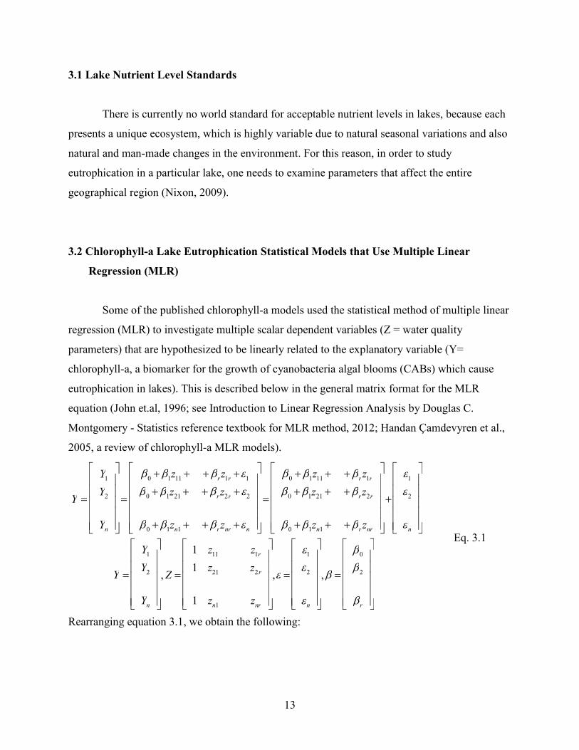
Some of the published chlorophyll-a models used the statistical method of multiple linear

regression (MLR) to investigate multiple scalar dependent variables (Z = water quality

parameters) that are hypothesized to be linearly related to the explanatory variable (Y=

chlorophyll-a, a biomarker for the growth of cyanobacteria algal blooms (CABs) which cause

eutrophication in lakes). This is described below in the general matrix format for the MLR

equation (John et.al, 1996; see Introduction to Linear Regression Analysis by Douglas C.

Montgomery - Statistics reference textbook for MLR method, 2012; Handan Çamdevyren et al.,

2005, a review of chlorophyll-a MLR models).

Eq. 3.1

Rearranging equation 3.1, we obtain the following:

Y

Y

Y

Y

1

1

Y

Y

2

2

Y

Y

n

n

,

Z

0

1

z

1

1

z

1

1

1

z

1

r

1

z

r

2

z

1

1

r

z

2

r

1

0

1

1

z

z

n

2

1

1

z

n

r

r

z

2

r

2

0

1

z

,

n

1

1

2

r

z

n

n

r

n

,

0

0

2

1

r

z

1

1

r

z

1

r

0

1 z 2 1

r z 2 r

0

1 z n 1 r z n r

1

2

n

14

Eq. 3.2

Where, Y is an n-by-1 vector of responses, β is a m-by-1 vector of coefficients, Z is the

n-by-r design matrix for the model, ε is an n-by-1 vector of errors, is the output or dependent

variable, and are the independent or input variables. The short version of the general

MLR format is written as follows:

Eq. 3.3

In this type of chlorophyll-a (MLR) model, chlorophyll- a (Chla) is the dependent

variable. representing: total phosphorus, total nitrogen, chloride, secchi depth, temperature,

depth, alkalinity or the independent variables (water quality parameters), while

represent the coefficients for the independent variables and ε is the error term.

The MLR equation is solved using the least squares method, by estimating the unknown

vector of coefficients β of the linear equation, through minimizing the sum of squares of

residuals (errors) between the observed data and the predicted data from the linear equation. The

coefficients β that produce the best solution are found when the error between the linear equation

model and observed data is zero (Kariya et al., 2004). By setting ε= 0 and rearranging the

equation, we get β=S(β)/Z, which give the coefficients of matrix β, and the predicted values. By

comparing the predicted values to the observed values we can judge the model’s accuracy. It is

not possible to directly evaluate the coefficients of the matrix β equation since the vector S(β) has

a different vector size than the matrix Z. Therefore, in appendix B, I wrote a Matlab code called

MLR-LEF to work around this problem, and use this code in the Lake Champlain case study.

Y

1 z 1 1 z

1 r

1 z 2 1 z

2 r

1 z n 1 z

n r

0

1

r

1

2

n

Z

15

3.3 Chlorophyll-a Lake Eutrophication Models that Use Multiple Nonlinear Regression

(MNR)

Some of the chlorophyll-a models (Handan et al., 2005 and Xia et al., 2011) use multiple

nonlinear regression (MNR) to investigate variables (water quality parameters) that are not

linearly related to chlorophyll-a and CABs (Nonlinear Regression by G. A. F. SEBER -Statistics

textbook ref for MNR; see refs above for chlorophyll-a MLR models). The multiple nonlinear

regression model is derived by transforming the nonlinear model to a linear one, the general

Nonlinear multivariate power function (Allison, 1999) is written as

Eq. 3.4

By taking the natural logarithm for both sides, equation 3.4 is then transformed into a linear

function (Allison, 2006)

( ) ( ) ( ) ( ) Eq. 3.5

Comparing Eq. 3.3 to Eq. 3.5 we get

( ) ( ) Eq.3.6

Equations 3.5 and 3.6 can be used to derive the chlorophyll-a MNR model (Handanet al., 2005

and Xia et al., 2011).

3.4 Chlorophyll-a Models that Use Data Mining (DM)

Data mining (DM) is used to discover patterns within a data set (Weiss et al., 1999;

Malek et al., 2011). A number of published chlorophyll-a models use DM to discover patterns in

data sets of water quality parameters (independent variables) that are related to chlorophyll-a

levels (dependent variable), a biomarker for CABs growth. For example DM was used in a

chlorophyll-a model to examine habitat utilization patterns of reef fish along the West coast of

Hawaii (Kleiner et al., 2000; Bailey et al., 1994). The software used in this study for data mining

16

is Eureqa 1.12.1 Beta from Nutonian. Eureqa software derives the equations by searching the

space of mathematical expressions to find the model that best fits a given dataset, both in terms

of accuracy and simplicity, this process is known as Symbolic Regression (SR), and unlike

multiple nonlinear regression MNR where a specific equation is need to start with the analysis, in

Symbolic Regression no particular model is needed to start with the analysis and the initial

expressions are formed randomly by combining mathematical building blocks such as

mathematical operators, analytic functions, constants, and state variables. Equations are then

build by recombining previous equations, using genetic programming, by letting the patterns in

the data reveal the suitable models, rather than imposing a model to avoid human bias, or

unknown gaps in domain knowledge.

3.5 Chlorophyll-a Model Evaluation Techniques

To find the best chlorophyll-a model for the Lake Champlain case study, I used three

published methods to evaluate chlorophyll-a models, and these are described in detail below.

3.5.1 Determination of coefficient

This method was used to evaluate most chlorophyll-a models used in lake eutrophication

studies, (e.g. Handan et al., 2005; Xia et al., 2012). The Pearson R correlation coefficient

measures the linear correlation between two variables (value between +1 and −1). R2 (the square

of the Pearson R) indicates how close the regression model fits to the observed data (value

between 0 and 1).

∑ ( )

∑ ( )

Eq. 3.7

Where, the coefficient of determination, Ŷ is the predicted value, is the observed

value, Y is the average value, n = the size of the data. The closer the R2

value is to 1, the better

the model fit. Fig. 3.1 shows two examples where this is not the case.

17

Figure 3.1 R2for unfit models (modified from http://academic.uprm.edu/accessed on May 2014)

The major problem in calculating R2

is that its value increases whenever a new variable is

added to the model, thus a model with more variables may appear to be a better fit than a model

with fewer variables. The adjusted R2

attempts to compensate for the inaccuracy of R2

because it

increases only if the new variable is statistically significant. The adjusted R2

is always less than

R2 (Draper et al., 1998).

(( )( )

) Eq. 3.8

Where is the adjusted coefficient of determination, is the coefficient of

determination, n is the total sample size, k is the number of predictors (variables).

3.5.2 Standard error of the estimate

This method was used in the verification analysis of Lake Ontario (Thomann et al., 1979).

The standard error of the estimate is an estimate of the average squared error and is calculated as

follows (Kenney et al., 1963).

√ √

√∑ ( )

Eq. 3.9

18

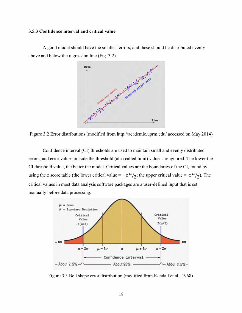
3.5.3 Confidence interval and critical value

A good model should have the smallest errors, and these should be distributed evenly

above and below the regression line (Fig. 3.2).

Figure 3.2 Error distributions (modified from http://academic.uprm.edu/ accessed on May 2014)

Confidence interval (CI) thresholds are used to maintain small and evenly distributed

errors, and error values outside the threshold (also called limit) values are ignored. The lower the

CI threshold value, the better the model. Critical values are the boundaries of the CI, found by

using the z score table (the lower critical value = ⁄ ; the upper critical value = ⁄ ). The

critical values in most data analysis software packages are a user-defined input that is set

manually before data processing.

Figure 3.3 Bell shape error distribution (modified from Kendall et al., 1968).

19

An alternative method to find z score is to use MS excel command line to calculate the z

value, which can be calculated using the following command

=NORMSINV(x) Where x is the value that we want to find its z score

3.6 GIS Based Modeling and Assessment

The Geographical Information System (GIS) is combination of software, data and

hardware that allow the user to query, visualize, and interpret spatial information to disclose

relationships, trends, and patterns within a data set. ArcGIS, developed by Environmental

Systems Research Institute (ESRI) is the most commonly used GIS package utilized by

researchers community for business analysis, planning, environmental applications and

geostatistical analysis. (See GIS Software - a description in 1000 words by Stefan Steiniger,

2009). The components (objects) in ArcGIS represent water quality monitoring stations and

other real world objects. The objects used in the Lake Champlain case study were the over 50

water quality monitoring stations located throughout the lake. The objects are stored in the

ArcGIS Geodatabase, which is the top-level element in the ArcGIS hierarchy, shown in figure

3.4. The hierarchical data structure allows feature classes to inherit the attributes and behaviors

of the object above while retaining its spatial properties (Zeiler, 1999).

20

Figure 3.4 GIS hierarchy (modified from http://webhelp.esri.com; accessed on Jan 2014).

Geostatistics analysis will produce the same modeling results as MLR if location has no

impact on the lake dataset. The ordinary least square (OLS) regression method, which is the

multi linear regression method used in ArcGIS, was used to test the significance of the location

of the lake variables. If location is an important independent variable for the Lake Champlain

study, then geographically weighted regression (GWR) tool from ArcGIS is used where location

is considered as an independent input variable that affects the model. In the final stage of the

analysis, the spread and distribution of the pollutant (chlorophyll-a) and of the variables (water

quality parameters) was determined by creating maps using the Empirical Bayesian Kriging

(EBK) method.

21

Figure 3.5 Lake Champlain eutrophication modeling using the GIS integrated analysis approach

22

CHAPTER 4

CASE STUDY: LAKE CHAMPLAIN

23

4.1 An Overview of Lake Champlain

This lake is one of the largest glacially formed lakes in North America (see figure 4.1). It

is situated partially in Vermont and NY states, USA, and partially in Quebec, Canada. Its

approximate dimensions are: L=193 km, maximum width =30 km, watershed =21 km2, surface

area =1100 km2, maximum depth =122 m (most is shallow =1.5 m), mean depth =19 m. The lake

has 5 different environmental zones (http://www.lakechamplaincommittee.org/learn/natural-

history-lake-champlain, accessed on Dec 2014). The five major segments of the lake are:

The South Lake, which is long skinny and shallow.

The Main Lake, which is the deepest and widest section of the lake.

Malletts Bay circumscribed by historical railroad and road causeways.

The Inland Sea, which lies to the east of the Hero Islands.

The Missisquoi Bay and is a large and discrete bay rich with wildlife.

This geography was used in the case study to improve the results of the multiple linear

regression and in data mining classification analysis.

No. Variables Definition

1 Chlorophyll-a (Chla)

(μg/L) Biomarker for Cyanobacteria algal blooms (CABs)

Lak

e C

ham

pla

in w

ater

shed

man

agem

ent

20

13

2 Total Phosphorus (TP)

(μg/L)

Pollutant from agriculture and industry, a nutrient for

CABs growth

3 Chloride (Cl) (μg/L) A highly reactive gas, used as a disinfectant in water

Treatment

4 Secchi Depth (Secchi)

(m)

Measure of water clarity/turbidity, a physical indicator

of bacterial growth

5 Total Nitrogen (TN)

(μg/L)

Pollutant from wastewater from agriculture and industry,

a nutrient for CABs growth.

6 Temperature (T)(oC) Surface temperature

7 RegAlk

The quantitative capacity of an aqueous solution to

neutralize an acid

8 Depth (m) Monitoring stations sampling depth

Table 4.1 Names, abbreviations and definition of water quality monitoring parameters (variables)

used in the LEF modeling studies, using Lake Champlain data.

24

Figure 4.1 Lake Champlain watershed (modified from Hegman et al., 1999).

25

4.2 Raw Data and Variables for the Lake Champlain Case Study

Environmental stress on Lake Champlain started in the early 1980s when phosphorous

levels from agricultural runoff and municipal sewage treatment plants caused excessive

cyanobacteria algal blooms (CABs), which resulted in drinking water contaminated by

trihalomethanes (THMs) produced by the CABs, and the presence of nuisance plant species such

as the genus Salvinia and a wide range of Cyanobacteria algae (Amsterdam et al., 2005). The

water quality parameters (variables) used in my modeling studies are shown in Table 4.1 above,

together with their abbreviations and definitions. The source of the data on water quality

parameters (including chlorophyll-a concentrations) used in the present study was from the state

of Vermont, which decided to share Lake Champlain’s environmental data with the public to

help researchers conduct studies that could provide solutions for the lake’s problems (Vermont

Agency of Natural Resources, 2011). This data included information on total maximum daily

loads of pollutants, available to the public and researchers via the Lake Champlain watershed

management web site (www.watershedmanagement.vt.gov), accessed for this thesis project on

Dec 2012.

Section 303(d) of the Federal Clean Water Act 1972 obligated all states in USA to

identify waters for which wastewater effluent did not attain water quality standards. In 1998, the

US Environmental Protection Agency (USEPA) defined the total maximum daily loads

(TMDLs) framework for determining acceptable levels of nutrients in fresh water lakes.

According to the 2001 Clean Water Action Plan, Vermont had to determine the TMDLs for the

pollutants causing water problems in Lake Champlain and present a study with proposed

solutions (Lake Champlain Phosphorus TMDL, 2002).

4.3 Lake Quality Criteria

Global drinking water guidelines are based on the world health organization (WHO).

According to WHO, the provisional value for cyanobacteria concentration in drinking waters is

1.0 μg/L. However, WHO does not provide any criteria for the acceptable levels of total

phosphorus or nitrogen concentration within lakes, rivers or reservoirs.

26

In the United States, there are no federal regulatory guidelines for cyanobacteria (algae)

concentrations in water (EPA-810F11001, 2012). However, section 303(d) of the Federal Clean

Water Act obliges each state to distinguish waters for which wastewater effluent limitations are

not sufficient to attain the quality standards, and to suggest solutions based on studies and filed

data analysis to obtain the required funding to solve the water problem. The water quality

standards and criteria change from one lake to another, even within a single lake we may see

different criteria, and a good example for that is lake Champlain, where there are various criteria

within lake Champlain due the difference in the hydraulic retention time between the lake

segments where the time varies from two months to three years, resulting in significant

difference in the nutrient distribution within the lake basin. The standards and criteria set for

Lake Champlain were derived from: 1) Trophic categorization schemes for lakes (e.g. Table

4.2); 2) Lake user survey and analyses between predicted and recorded values for total

phosphorus (TP) concentrations (Smeltzer, 1999); 3) The 1993 Water Quality Agreement, which

establish TP targets for 13 segments of Lake Champlain.

Selected Lake Champlain Water

Quality Monitoring Stations

Depth

(m)

Current Level

(2011)

Criteria Targets

TP μg/L Chla μg/L TP μg/L Chla μg/L

02 - South Lake B 5 52 10557 25

No d

efin

ed c

rite

ria

04 - South Lake A 10 47 16677 25

07 - Port henry Segment 50 21 6374 14

09 - Otter Creek Segment 97 18 6177 14

16 - Selburne Bay 25 16 5830 14

19 - Main Lake 100 16 4836 10

21 - Burlington Bay 15 16 4961 14

25 - Malletts Bay 32 15 2928 10

33 - Cumberland Bay 11 20 4568 14

34 - Northeast Arm 50 23 4250 14

36 - Isle LaMotte (off Grand Isle) 50 18 3043 14

40 - St. Albans Bay 7 31 5770 17

46 - Isle LaMotte (off Rouses Pt) 7 21 3941 14

50 - Missisquoi Bay 4 50 10658 25

51 - Missisquoi Bay Central 5 53 16196 25

Table 4.2 Lake Champlain phosphorus criteria targets 2011 vs. observed values for the same year

(updated and modified from Lake Champlain Phosphorus TMDL, 2002).

27

Tab

le 4

.3 L

ake

trophic

cri

teri

a, S

ourc

e: (

Lit

erat

ure

rev

iew

rel

ated

to s

etti

ng n

utr

ient

obje

ctiv

es f

or

lake

Win

nip

eg, 2006)

28

The way criteria levels were decided for Lake Champlain segments was explained in the

Vermont DEC (1990) as well as in Lake Champlain basin program (1996), and is summarized as

follows:

Main Lake and Mallets Bay segments are large central broad areas with low nutrient

level; therefore an oligotrophic standard of 0.010 mg/L phosphorus is desirable for these

two segments.

In the remaining parts of the lake, the phosphorus concentrations are significantly higher

than 0.010 mg/L, consequently the attainability for these segments to oligotrophic

criterion is doubtful. Therefore, higher criteria level of 0.014 mg/l was chosen for the rest

of the lake (except for St. Albans Bay, Missisquoi Bay, and the South Lake). The mean

value of 0.014 mg/L represents a phosphorus level at which an algae nuisance condition

would be present only 1% of the time during the summer.

St. Albans Bay, Missisquoi Bay, and the South part of the lake are highly eutrophic

segments; therefore the target of 0.014 mg/l criteria would not be realistically attainable.

There have been many attempts in St. Albans to reduce phosphorus levels including

treatment plant upgrades and nonpoint source controls. The water quality set by the

Vermont department of environmental conservation (DEC) in the St. Albans Bay aim is

to reduce the phosphorus in the center bay area to a concentration of about 0.003 mg/l

above the level outside the bay in the Northeast arm. Thus, a phosphorus criterion of

0.017 mg/l was selected for St. Albans Bay.

Missisquoi Bay and the South lake segments are shallow depth and have wetland like

characteristics therefore, they are considered as naturally eutrophic (high nutrient) areas.

The high eutrophic state in Missisquoi Bay area has beneficial values for productive

warm-water fisheries and wildlife habitats. Therefore, a phosphorus criterion of 0.025

mg/l reflecting a moderate level of eutrophication was selected for these segments.

Recent and historical phosphorus and cyanobacteria concentrations in lake Champlain

have exceed the desired criteria levels. In many cases the recorded values were more than

double of the desired criteria. Figure 4.2 shows the phosphorus levels in Lake Champlain

compared with water quality criteria.

29

Figure 4.2 Phosphorus levels in Lake Champlain and water quality criteria (Lake Champlain

Phosphorus TMDL, 2002).

30

4.4 Data Collection and Quality Analysis

The process of data entry and acquisition is inherently prone to errors and the raw data

from the Lake Champlain monitoring stations did not reveal much information. A thorough data

preparation and cleansing was required before starting with modeling and statistical analysis.

A -Data source, format and units

The process of Lake Champlain monitoring station data entry and acquisition is

inherently prone to errors; lake Champlain’s data is available in its raw format through the lake

Champlain long-term water quality program. After downloading the data, it is then sorted and

transformed into one file of MS excel. To simplify the analysis all the concentrations for the

different water quality parameters are unified and converted to μg/L.

B -Data quality analysis

For Lake Champlain, data quality control is implemented through the Vermont

department of environmental conservation (DEC), while for this research data quality control is

implemented through filtration of outliers and working with averages.

C -Monitoring frequency

Since 1992 volunteers helped collecting the data for Lake Champlain between 1992 and

2011. The database contained 12,994 records for 33 variables. Table 4.4 lists the variables, their

monitoring range and frequency while figure 4.3 shows the location of the monitoring stations.

31

Variables Code Units Date Range Lab Sampling Frequency

Total Phosphorus TP μg/L 1992 - 2011 VT and

NY 10/year

Dissolved Phosphorus DP μg/L 1992 - 2011 VT and

NY 10/year

Ortho-Phosphorus DOP μg/L 1992 - 1994 VT and

NY -

Chloride Cl mg/L 1992 - 2011 VT and

NY 10/year

Dissolved Silica DSi mg/L 1992 - 2011 VT and

NY 10/year on a 5 yr cycle

Total Nitrogen TN mg/L 1992 - 2011 VT 10/year

Total Kjeldahl Nitrogen TKN mg/L 1992 - 1996 NY -

Total Nitrate-Nitrite TNOX mg/L 1992 - 1996 VT and

NY -

Total Ammonia TNH3 mg/L 1992 - 1996 VT and

NY -

Calcium TCa mg/L 1992 - 2011 VT and

NY 3/year on a 5yr cycle

Magnesium TMg mg/L 1992 - 2011 VT and


Sodium TNa mg/L 1992 - 2011 VT and


Potassium TK mg/L 1992 - 2011 VT and


Iron TFe μg/L 1992 - 2010 VT and


Lead TPb μg/L 1992 - 1998 NY -

Total Organic Carbon TOC mg/L 1992 - 1999 NY -

Dissolved Organic Carbon DOC g/L 1992 - 1999 NY -

Dissolved Inorganic

Carbon DIC mg/L 1992 - 1996 NY -

Temperature TempC deg C 1992 - 2011 VT 10/year

Dissolved Oxygen DO mg/L 1992 - 2011 VT 10/year

Conductivity Cond μS/cm 1992 - 2005 VT 10/year

pH pH - 1992 - 2005 VT 10/year

Alkalinity RegAlk mg/L 1992 – 2011 VT 3/year

Total Suspended Solids TSS mg/L 1992 – 2005 VT and

NY -

Chlorophyll-a Chla μg/L 1992 – 2011 VT and

NY 10/year

Secchi Depth Secchi m 1992 – 2011 VT and

NY 10/year

Table 4.4 Lake Champlain variables and their monitoring range and frequency

(Lake Champlain Phosphorus TMDL, 2002).

32

Figure 4.3 Lake Champlain monitoring stations (www.vtwaterquality.org; accessed on Jan 2014)

33

D -Gaps and range

Some of the reasons that contributed to problems within the lake data were:

Monitoring stations for Lake Champlain were introduced over different periods of time.

New variables are being introduced while others were dropped.

The collection of the variables was not made concurrently as would be desirable for the

purpose of analyzing ecological interrelationships.

As a result, the monitoring periods vary between the lake variables and between one

station and another, therefore the lake daily data is full of gaps and missing ranges. For example

out of the 12,994 data records for lake Champlain, not a single row contained a complete set of

concurrent reading for a set of variables. This was a major setback, since empty cells typicall are

dropped or interpolated during analysis, another challenge is that : the gaps and missing ranges

for several variables exceeded 20 months, thus making interpolation, or exploration a difficult

task. Table 4.5.of the yearly data for station 07 Port Henry of Lake Champlain, illustrate the

extent of the gaps problem.

Year Depth TP Cl TN TCa Minerals Toxic TOC TempC DO pH Secchi RegAlk Chla

1992 50 13.58 11742 509.58 13847.44 22 4.3 16.54 7.98 4.33 53.91 5.63

1993 50 18.25 11501 456.79 12804.96 15.75 3.95 23.5 7.67 3.63 54.3 5.25

1994 50 15.78 11987 460.9 12608.9 22.72 8.84 22.16 7.21 3.68 53.55 5.27

1995 50 10.33 13175 384.44 11718.8 5.2 15.3 15.75 10.18 7.54 5.23 53.02 3.05

1996 50 13.88 12524 445.33 12156 5 4.75 16.48 9.96 7.91 4.06 51.1 4.44

1997 50 13.23 12184 454.4 13140.5 5.13 3.33 24.02 10.53 7.8 4.27 53.9 4.78

1998 50 13.75 12076 438.5 10367.67 5 4.86 17.12 10.28 7.77 3.96 54.6 4.72

1999 50 13.39 12641 460.33 14121 3.56 19 10.39 7.82 4.92 50.41 6.83

2000 50 15.31 12575 451.25 14322.13 25.86 10.32 7.72 4.22 51.62 5.98

2001 50 12.93 13163 479.83 14695.25 23.18 10.54 7.74 4.47 53.23 3.49

2002 50 10.59 13979 400.6 15113 17.84 10.15 7.78 5.03 51.63 1.82

2003 50 12.92 15093 433.39 15717.7 25 10.42 7.84 4.95 51.23 5.46

2004 50 16.44 14981 412.08 16243.6 23.68 10.2 7.91 4.4 51.95 5.45

2005 50 16.36 15344 410.54 14793.88 12.18 10.41 7.84 3.1 52.6 10.34

2006 50 17.13 14582 438.3 20.54 10.06 3.46 54.53 6.17

2007 50 14.61 13843 438.02 18.43 10.34 4.05 51.91 4.92

2008 50 18.69 14720 444.25 8.7 10.22 3.6 53.36 4.8

2009 50 16.64 14583 407.57 22.9 10.8 3.47 55.5 4.9

2010 50 16.5 14155 363.72 15286.75 13.1 10.29 3.55 57.13 4.87

2011 50 22.12 12926 405.12 15466.67 21.98 10.21 2.66 55.32 6.25

Table 4.5 Port Henry segment (07) of lake Champlain observed data.

34

I presented table 4.5 with the yearly data since it was easier to show the extent of the

problem, however, I started the analysis using the daily data, where the problem is greater. The

biggest challenge is that for the Lake Champlain data, each water quality monitoring station

exhibits a set of different problems with their variables, and due to the size of the gaps and long

missing ranges within the data set, interpolation or extrapolation does not work. As an alternative,

I decided to analyze the distribution of the data in order to reveal trends, to make estimating the

gaps and missing ranges easier. Trends can be investigated either visually or using statistical

tests like Mann–Kendall. Previous studies indicate that this approach is likely to see curves and

nonlinear shapes of the data for water quality parameters, rather than straight lines. Figure 4.4

shows the different types of nonlinear curves that we may expect to see in a data set.

Figure 4.4 Nonlinear curve types (http://epa.gov/ncct/edr; accessed in June 2014)

A monotonic curve consistently stays in one direction (either always upwards or always

downwards), while a nonmonotonic curve keeps changing its direction (G. Brewka, 1991).

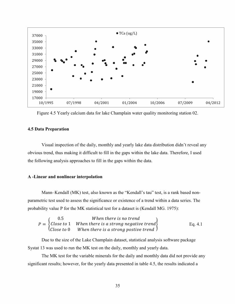
Figure 4.5 shows the yearly Calcium observed data for monitoring station 02 (South Lake B);

again I used yearly data to show the extent of the problem. Within the data there is 36 months

gap between 1992 and 1995, such gap can be clearly seen on the graph, at the same time the data

seems to take a non-monotonic distribution throughout the recorded range.

35

Figure 4.5 Yearly calcium data for lake Champlain water quality monitoring station 02.

4.5 Data Preparation

Visual inspection of the daily, monthly and yearly lake data distribution didn’t reveal any

obvious trend, thus making it difficult to fill in the gaps within the lake data. Therefore, I used

the following analysis approaches to fill in the gaps within the data.

A -Linear and nonlinear interpolation

Mann–Kendall (MK) test, also known as the “Kendall’s tau” test, is a rank based non-

parametric test used to assess the significance or existence of a trend within a data series. The

probability value P for the MK statistical test for a dataset is (Kendall MG. 1975):

{

} Eq. 4.1

Due to the size of the Lake Champlain dataset, statistical analysis software package

Systat 13 was used to run the MK test on the daily, monthly and yearly data.

The MK test for the variable minerals for the daily and monthly data did not provide any

significant results; however, for the yearly data presented in table 4.5, the results indicated a

17000

19000

21000

23000

25000

27000

29000

31000

33000

35000

37000

10/1995 07/1998 04/2001 01/2004 10/2006 07/2009 04/2012

TCa (ug/L)

36

significant P value for both upward and downward trends, indicating a two-sided trend. The MK

test also indicated that the upward trend better describes the general data distribution.

The Systat 13 software detected the gaps within the data using the MK test: the gap in the

middle of the series from 2005 till 2010, and the missing values for the years of (2006, 2007,

2008 and 2009). Systat 13 automatically interpolated these gaps, and the interpolation was

completed using local quadratic smoothing as shown in figure 4.6.

Figure 4.6 The Mann–Kendall test and the interpolation.

This interpolated gap approach is typical of many software packages; they either fill the

gaps or completely ignore the missing range. The gap in the mineral variables yearly data was

common across all the monitoring stations; hence it wasn’t possible to verify the results. I

compared the minerals data distribution against other variables, which did have a complete data

range. I scaled the TP and Cl variables data records up to fit within the same range as the

minerals dataset, and the results are plotted in figure 4.7. I noticed that in the gap period, the

datasets for both TP and Cl exhibited a non-monotonic behavior, while the interpolated data

range for minerals, which was done using the MK test, was a straight line. Additionally, before

and after the range, the datasets for all three variables had non-monotonic behavior. This

provided enough evidence to raise doubts about the interpolated results and to stop the

investigation using MK trend analysis as a tool to fill in the gaps and to predict the missing data

ranges.

37

Figure 4.7 Yearly TP, Cl and minerals chart for lake Champlain Port Henry

Further investigation of the lake data shows that the lake variables have a non-monotonic

data distribution therefore; linear interpolation or extrapolation was not an option.

An earlier study of Lake Champlain suggests that using mean values of water quality

parameters produced a relatively high degree of statistical precision (Smeltzer, et al., 1989). By

using the mean values we remove many of the unwanted gaps, therefore daily data for Lake

Champlain was averaged to produce monthly data, however the monthly data also had several

gaps and missing range, so the investigation and the data cleansing process continued on the

monthly data. To avoid presenting redundant results, I skipped presenting the analysis for the

daily and monthly data, although I have thoroughly investigated each set, and I directly used the

yearly data throughout the rest of the thesis. However, even the yearly data still had gaps and

missing ranges, so I used the approach described below to complete the ranges and fill in the

gaps for the yearly data of Lake Champlain, in order to avoid dropping a variable from the

analysis.

Assuming we manage to get the information about the equation that best describes the

data distribution over a significant period, then it is possible to use the function to estimate the

gaps and missing range within the data (Zhu et al., 2003). These authors proposed using discrete

Fourier transform for time series data, while other studies (Xiang and Gray, 1999) suggested

9000

10000

11000

12000

13000

14000

15000

16000

17000

18000

19000

1990 1995 2000 2005 2010 2015

TP Cl Minerals

38

using Fuzzy logic or recommend neural networks. FindGraph data mining software package is a

tool that facilitates the search through 10s of different functions (e.g. Linear Regression, Fourier,

Polynomial, Exponential, Logarithm, Power and Waveform) to produce models that fit the data

under investigation.

Figure 4.8 is a screen shot of FindGraph software during the setup process; the screen

shot reveals the different available time series functions that were used to estimate the Lake

Champlain water quality monitoring data distribution.

Figure 4.8 Data mining (FindGraph) analysis.

The variable minerals data from table 4.5 was used for the test run, but this time the data

was split into two halves: the first half (years 1992 till 2001) was used to generate the time series

model; while the second set (between 2002-2011) was used to verify the model. FindGraph

software investigated more than 999,999,999 iterations in less than 2 minutes. Several models

were generated and were sorted according to their best R2. The best curve fit model that

represented the minerals data distribution between 1992 till 2001 was a Fourier function with 3

harmonics.

39

Minerals(t)= 12603.92 +(804.73*cos(0.78*t) +76.33*sin(0.78*t)

+(773.25*cos(1.57*t) + 26.41*sin(1.57*t)) +(74.06*cos(2.35*t) -

1044.27*sin(2.35*t)

Eq. 4.2

Figure 4.9 Data mining (FindGraph) results.

Figure 4.9 shows the Fourier function with 3 harmonics as found by FindGraph software

and in figure 4.10 the actual recorded data for minerals from table 4.5 is plotted against the

Fourier time function for comparison.

Figure 4.10 Minerals Fourier predictions for station 02

10000

11000

12000

13000

14000

15000

16000

17000

1990 1995 2000 2005 2010 2015

Minerals Predicted Minerals (Fourier model)

40

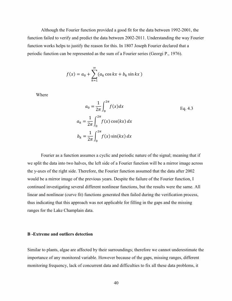
Although the Fourier function provided a good fit for the data between 1992-2001, the

function failed to verify and predict the data between 2002-2011. Understanding the way Fourier

function works helps to justify the reason for this. In 1807 Joseph Fourier declared that a

periodic function can be represented as the sum of a Fourier series (Georgi P., 1976).

( ) ∑( )

Where

∫ ( )

∫ ( ) ( )

∫ ( ) ( )

Eq. 4.3

Fourier as a function assumes a cyclic and periodic nature of the signal; meaning that if

we split the data into two halves, the left side of a Fourier function will be a mirror image across

the y-axes of the right side. Therefore, the Fourier function assumed that the data after 2002

would be a mirror image of the previous years. Despite the failure of the Fourier function, I

continued investigating several different nonlinear functions, but the results were the same. All

linear and nonlinear (curve fit) functions generated then failed during the verification process,

thus indicating that this approach was not applicable for filling in the gaps and the missing

ranges for the Lake Champlain data.

B -Extreme and outliers detection

Similar to plants, algae are affected by their surroundings; therefore we cannot underestimate the

importance of any monitored variable. However because of the gaps, missing ranges, different

monitoring frequency, lack of concurrent data and difficulties to fix all these data problems, it

41

makes sense to shift the analysis to the yearly timeframe. Yearly data is obtained by averaging

monthly data, and the monthly data was obtained by averaging the daily data. The daily data

records for the lake water quality parameters were inconsistent, and some months had barely a

single data entry, while other months had tens of data records. This problem presents a risk of

having the results deviating by one or two extreme values. For example let us assume the

following data records for a lake segment.

Data for

1997 Total Phosphorus readings (μg/L)

Number of Daily

data records

March 10 11 9 3

April 14 15 13 9 4

May 11 11 2

June 12 14 10 17 8 5

July 15 11 8 13 17 5

August 12 12 10 16 11 17 6

September 65 1

October 10 14 2

To find total phosphorus typical value for each month, we average the data for that month,

for example, on June the monthly average were = (12+14+10+17+8)/5 = 14.8 μg/L. In the same

way we find the average for the other months.

March = 10 July = 12.8

April = 12.75 August = 13

May = 11 September = 65

June = 12.2 October = 12

To obtain the yearly data we average the monthly data, the 1997 yearly data

=(10+12.75+11+12.1+12.8+13+65+12)/7 = 18.59, the question is: was the extreme data record

for the month of September a result of human error? Assuming it was an error and dropping it

from the analysis will give the following yearly data =(10+12.75+11+12.1+12.8+13+12)/6=

11.96, such a significant difference can be the deciding factor for a lake to meet the federal

TMDL criteria or not. If in each year on the same month of September we had similar extreme

value, then in this case such a value becomes seasonal high record and is not considered as an

anomaly. To judge whether a data record is extreme or not, we must run seasonal tests or

visually inspect the overall data distribution. Many methods are available for detecting outliers or

extreme values, the simplest of these is to visually screen the data, and typically outliers are

spotted at the border of data distribution. For example in figure 4.11 the majority of the daily

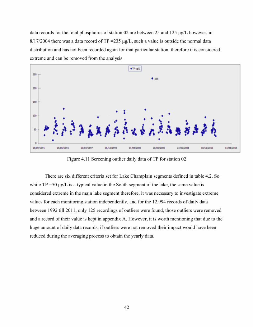
42

data records for the total phosphorus of station 02 are between 25 and 125 μg/L however, in

8/17/2004 there was a data record of TP =235 μg/L, such a value is outside the normal data

distribution and has not been recorded again for that particular station, therefore it is considered

extreme and can be removed from the analysis

Figure 4.11 Screening outlier daily data of TP for station 02

There are six different criteria set for Lake Champlain segments defined in table 4.2. So

while TP =50 μg/L is a typical value in the South segment of the lake, the same value is

considered extreme in the main lake segment therefore, it was necessary to investigate extreme

values for each monitoring station independently, and for the 12,994 records of daily data

between 1992 till 2011, only 125 recordings of outliers were found, those outliers were removed

and a record of their value is kept in appendix A. However, it is worth mentioning that due to the

huge amount of daily data records, if outliers were not removed their impact would have been

reduced during the averaging process to obtain the yearly data.

43

C -Selecting data range and variables

Water quality monitoring of Lake Champlain at particularly stations (i.e. stations 2, 4, 7,

19, 21, 25, 33, 34, 36, 40, 46, 50) started in 1992, while monitoring for stations 9 and 16 didn’t

start till later in 2001, and station 51 was added in 2006. Typically, earlier data is used for

training while recent data is used for testing. Applying this approach means that data from

stations 9, 16 and 51) will not be included in the model creation.

Therefore throughout this study for Lake Champlain, data between 2003- 2011 will be

used for model creation, while the data between 1992- 2002 will be used for verification. The R2

value increases whenever a new predictor is added, so a model with more variables will appear

to be a better fit than a model with fewer variables. Thus, it is to our advantage to include as

many variables as possible, although the gaps in the Lake Champlain data resulted in dropping

few variables. The variables selected for this thesis are listed in table 4.6.

Variable name Code Units Date Range Lab Sampling Frequency

Total Phosphorus TP μg/L 1992 – 2011 VT & NY 10/year

Chloride Cl mg/L 1992 – 2011 VT & NY 10/year

Total Nitrogen TN mg/L 1992 – 2011 VT 10/year

Temperature TempC deg C 1992 – 2011 VT 10/year

Alkalinity RegAlk mg/L 1992 – 2011 VT 3/year

Chlorophyll-a Chla μg/L 1992 – 2011 VT & NY 10/year

Secchi Depth Secchi m 1992 – 2011 VT & NY 10/year

Time Date Years 1992-2011

Depth Depth m 1992-2011

Table 4.6 Lake Champlain variables monitoring range (modified from lake Champlain

phosphorus TMDL, 2002).

In section 2.1.1 Phosphorus Cycle I emphasized on the importance of internal loading in

lake modeling analysis, however the lake Champlain data available through the long-term water

quality program does not have the internal loading, so I started the analysis of lake Champlain

assuming a negligible internal loading, which is a valid assumption for the majorly of the deep

monitoring stations.

44

Water quality parameters causing eutrophication and algae bloom depend on the same

factors, including the amount of rain, run off water and human activities, all of which result in a

strong correlation between the variables. To simplify the analysis, however, the water quality

parameters used for the analysis are assumed to be independent for the purpose of this thesis

project.

4.6 Modeling Steps

The objective of this thesis project was to better understand the importance of factors that

contribute to the growth of cyanobacteria algal blooms (CABs) in lake Champlain. I used the

approach illustrated in figure 4.12, which is explained below.

Firstly, I used historical data from the State of Vermont monitoring stations on lake

Champlain (www.watershedmanagement.vt.gov, accessed on Dec 2012), to investigate the links

between the levels of the seven selected independent water quality parameters (variables)

described in section 5.1, using a correlation matrix. This step determined the relative impact of

each variable on the dependent variable chlorophyll a levels (a biomarker for CABs). Secondly, I

investigated the compound impact of the water quality parameters on the CABs using modeling

techniques, including multiple linear regression (MLR), neural network (NN) and data mining

(DM). This step generated a number of chlorophyll a models. Thirdly, I verified each of the

chlorophyll models using recent data (as detailed in chapter 5) in order to find the best-fit model.

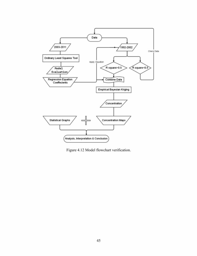
45

Figure 4.12 Model flowchart verification.

46

4.6.1 Multiple linear regression

Multiple linear regression (MLR) is a modeling technique which attempts to find the

relationship between several explanatory variables and a response variable, by fitting a linear

equation to the observed training data set, assuming we want to find the MLR for station 19 of

lake Champlain, we then use the yearly data presented in the following table. To avoid

potentially biased results, the data is split in two, the first half is used to derive the model while

the other half of the data is passed through the model equation and the output is compared with

the observed data for verification.

Station Year

Depth

(m) TP(μg/L)

Cl

(μg/L) TN (μg/L)

Secchi

(m)

Temp

C RegAlk

Chla (μg/L))

Data set

1

Z1 Z2 Z3 Z4 Z5 Z6 Z7 Z8 Y

19 1993 100 13.89 11495.00 433.75 5.13 14.02 51.57 3.33

19 1994 100 12.22 11594.44 466.33 5.33 12.68 49.50 4.33

19 1995 100 8.97 12661.11 452.22 6.41 9.80 52.41 4.16

19 1996 100 10.84 12461.70 447.08 4.88 8.90 50.38 4.04

19 1997 100 11.37 11733.89 453.33 4.87 12.00 50.45 4.61

19 1998 100 11.36 11879.17 396.25 5.20 12.53 50.37 3.86

19 1999 100 10.64 12310.26 444.05 6.57 21.67 49.03 4.70

19 2000 100 11.71 12622.00 427.17 6.04 16.78 49.14 3.66

19 2001 100 10.51 13099.00 430.50 5.46 19.98 49.26 3.43

19 2002 100 7.90 13633.33 403.67 6.50 22.24 48.20 1.52

Data set

2 19 2003 100 8.57 14706.25 409.33 6.87 21.06 48.23 2.91

19 2004 100 12.50 14775.28 398.50 6.11 16.53 49.31 3.62

19 2005 100 12.57 15118.33 409.47 4.84 19.34 51.48 5.34

19 2006 100 14.48 14686.31 435.12 4.42 19.60 49.83 4.34

19 2007 100 12.87 13760.00 432.58 4.94 19.18 49.84 3.32

19 2008 100 13.89 14448.33 436.00 5.40 18.20 49.42 3.34

19 2009 100 12.75 14293.06 410.14 5.62 18.03 51.32 2.90

19 2010 100 12.96 13975.71 370.29 4.60 13.00 53.72 3.10

19 2011 100 16.12 12978.10 387.19 3.48 6.10 51.35 4.62

Table 4.7 Lake Champlain yearly data for 1993-2011.

Solution: The concept of linear regression suggests the existence of a linear relationship

between the dependent variable (chlorophyll-a) and the independent variables listed above. In a

linear relationship the constant is the slope, so if we use part of the data to find the slope, then we

can use the other part of the data to verify the results. First the data in table 4.7 is split in half, the

first half will be used to derive the model (slope), and the second half will be used to verify the

model. The general format for the multiple linear regression model is

The above equation can also be rewritten in a matrix format using the lake variable as follows

47

Our target is to use half of the data set to find β and then use it to create the MLR

equation, then the model accuracy is evaluated by applying the MLR equation to the second half

of the data and comparing the model output with the observed data. The best MLR model is the

one where the error =0. Arranging the input and output variables from table 4.7 to match the

matrix equation results in:

[

]

[

]

Can be calculated from β=Y/Z when error=0, however, this computation is not directly

possible since Y and Z are of a different dimensions, so I developed a Matlab code LEF-MLR

(see appendix B) to obtain the following answers.

( ) [

]

For verification of the above model equation, we then used the data from the verification

data set 2; and the predicted values of Chla model are then compared to the observed monitoring

station values. The model was found to have R2= 0.0065, this is a low value, and this means that

our model isn’t of a good fit. Thus, the process is repeated again using a different set of input

variables, and this continues till a model with a good fit is found. The process of finding the right

input data set is a time consuming process, and we may not end up with the right set of variables,

because the input variables are highly correlated as seen from the correlation matrix.

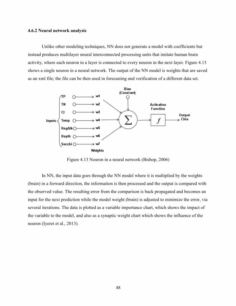
48

4.6.2 Neural network analysis

Unlike other modeling techniques, NN does not generate a model with coefficients but

instead produces multilayer neural interconnected processing units that imitate human brain

activity, where each neuron in a layer is connected to every neuron in the next layer. Figure 4.13

shows a single neuron in a neural network. The output of the NN model is weights that are saved

as an xml file; the file can be then used in forecasting and verification of a different data set.

Figure 4.13 Neuron in a neural network (Bishop, 2006)

In NN, the input data goes through the NN model where it is multiplied by the weights

(brain) in a forward direction, the information is then processed and the output is compared with

the observed value. The resulting error from the comparison is back propagated and becomes an

input for the next prediction while the model weight (brain) is adjusted to minimize the error, via

several iterations. The data is plotted as a variable importance chart, which shows the impact of

the variable to the model, and also as a synaptic weight chart which shows the influence of the

neuron (Iyeret et al., 2013).

49

4.6.3 Data mining

Also known as BLACK BOX MODEL, because it is computer written sophisticated

algorithms to reveal and extract hidden information from a data set (Maimon and Rokach, 2011,

Data Mining and Knowledge Discovery Handbook). Data mining technique is employed in this

study to:

A. Estimate the equations for the independent input parameters that were discontinued

from the monitoring program or newly introduced, in an attempt to fill the gaps

within the data.

B. Estimating the nonlinear regression equation of the combined chemical and biological

parameters for Chlorophyll-a.

4.6.4 Geostatistical analysis

ArcGIS version 10.1-geostatistical analysis package was used to investigate the impact of

lake location on cyanobacterial algal bloom in lake Champlain. Two files were needed for the

analysis are derived from:

1) Lake Champlain LTM QAPP/Work Plan Document Revision 1.4 provided the geographical

locations information for the monitoring stations.

2) The ArcGIS map shape file for lake Champlain, was partially available in the United States

USGS Water Resources web site (water.usgs.gov; accessed on Dec 2012). However, a big

section of the lake polygon was missing. Figure 4.14 shows a summary of the steps used to

create the lake polygon file, where firstly, the none relevant information was removed from the

USGS file, then USGS map was edited using the US topology map as a background image to

manually draw the missing parts for the northern and southern parts of the lake. Finally, the

entire lake shape was combined into one polygon for GIS analysis. The longitude and latitude

information was added to the lake data file and imported into ArcGIS.

50

Figure 4.14 Lake Champlain polygon creation.

Spatial analysis utilizes location information in the relationships, so if the data set under

investigation changes with location, then spatial analysis will reveal this information when

running the OLS regression test. The OLS tool is available through ArcToolbox menu from

ArcMap, If the location was found to be important then by using geographically weighted

regression (GWR) analysis, we can develop a linear regression model which will have the

location as one of its input variables. The OLS test is only valid when we have found the best

MLR model. OLS does not have the stepwise selection option which was available in SPSS, so

the OLS test does not know which set of input variables will produce the best regression model.

The variance inflation factor (VIF) value from the OLS test can help to determine if a

variable is important to the model or not, a VIF value > 7.5 indicates that the input variable is

redundant and should be omitted from the model. Although the OLS test does not consider the

location as an input, it automatically runs a test to determine the location importance for the

linear regression modeling. The Koenker statistic test is the one to determine the locations

importance: if the p-value <0.05, then the model equation is likely to change with the locations

across the study area. In this case we should consider the location as an input variable and use

GWR analysis instead.

Since stepwise selection is not available as in IBM SPSS, several iterations are need

before reaching significant a model. Alternatively, time can be saved by directly using the input

variables set obtained using the stepwise in IBM MLR

51

CHAPTER 5

LAKE CHAMPLAIN CHLOROPHYLL- A

STATISTICAL MODELING RESULTS

52

5.1 Correlation Matrix Analysis Results

The result of the cross correlation analysis are presented in table 5.1 and figure 5.1 for the

first part of the study, which examined the relationship and impact of seven independent water

quality parameters (variables; yearly data) on the dependent variable, chlorophyll-a (a biomarker

for cyanobacteria algal blooms; CABs) in lake Champlain.

VARIABLE YEAR DEPTH TP CL TN TEMPC SECCHI REGALK CHLa

YEAR 1.000

DEPTH -0.026 1.000

TP 0.096 -0.484 1.000

CL -0.243 0.125 -0.147 1.000

TN -0.086 -0.229 0.703 -0.398 1.000

TEMPC -0.064 -0.107 0.116 -0.085 -0.041 1.000

SECCHI -0.274 0.402 -0.894 0.088 -0.562 -0.117 1.000

REGALK 0.070 -0.130 0.432 0.731 -0.069 0.003 -0.460 1.000

CHLa 0.057 -0.341 0.803 -0.328 0.734 0.093 -0.757 0.127 1.000

Table 5.1 Pearson’s correlation matrix.

53

Fig

ure

5.1

Cro

ss c

orr

elat

ion s

catt

er p

lots

show

ing t

he

rela

tionsh

ip b

etw

een

the

8 i

ndep

enden

t w

ater

qual

ity v

aria

ble

s (l

ake

Cham

pla

in y

earl

y d

ata)

and t

he

dep

enden

t v

aria

ble

chlo

rophyll

-a (

at t

he

bo

ttom

). A

bbre

via

tions:

Dat

e, 1

992

-2011 (

YE

AR

); t

ota

l

phosp

horu

s (T

p);

Chlo

ride

(CL

); t

ota

l nit

rogen

(T

N);

tem

per

ature

in d

egre

es C

(T

EM

PC

); S

ecch

i dep

th (

SE

CH

I);

Alk

alin

ity

(RE

GA

LK

); c

hlo

rophyll

-a (

CH

LA

).

54

As expected, the cross correlation analysis indicated:

1) A significant strong positive linear relationship between the assumed independent variable

total phosphorus (TP; r=0.803), a nutrient for CABs growth (Correll, 1998), and the dependent

variable chlorophyll-a.

2) A significant strong positive linear relationship between the assumed independent variable

total nitrogen (TN; r=0.734), a nutrient for CABs growth (Correll, 1998), and the dependent

variable chlorophyll-a.

3) A significant strong negative linear relationship between the independent variable secchi

depth (r=-0.757), a measure of water clarity (Prescott, 2006) which is reduced by the growth of

CABs (George et al., 2010), and the dependent variable chlorophyll-a.

Also as expected, the analysis confirmed:

4) A significant strong positive linear relationship between two of the independent variables,

total phosphorus (TP) and total nitrogen (TN) (r=0.703), because they are both nutrients for

CABs growth (John A. Downing et al., 1992).

5) A significant strong negative linear relationship between the assumed independent variable

secchi depth (water clarity) and the assumed independent variable total phosphorus (TP; r=-

0.894).

6) A less significant trend towards a negative linear relationship between the assumed

independent variable secchi depth (water clarity) and the assumed independent variable total

nitrogen (TN; r=-0.562).

These results suggest that our modeling approach should be successful if we assume that

the levels of total phosphate (TP) and total nitrogen (TN) are indeed positively linearly related to

chlorophyll-a/CAB growth, and that conversely, secchi depth is negatively linearly related to

chlorophyll-a/CAB growth.

55

5.2 Determination of Analysis Data Set

I used MS Excel and Matlab to analyze lake Champlain yearly data over two different

time periods:

1) Early years yearly dataset: 1992-2002.

2) Later years yearly dataset: 2003 to 2011.

The early years and later years datasets were tested as either the training dataset or the

verification dataset for my modeling study, and the later years dataset worked better as a training

data set. This was because several new important monitoring stations were set up during the later

years time period, and the additional data from these stations improved the accuracy of the

models. Therefore, the later years yearly dataset was chosen for constructing the chlorophyll-a

models, and the early years dataset was used to verify the models.

5.3 Chlorophyll-a Modeling Using Multiple Linear Regression (MLR)

5.3.1 SPSS statistical analysis:

It is statistical software package that was used to analyze the lake Champlain later year

dataset as the model training dataset, with the critical value for the models = 95%, the error range

= -1.96 to 1.96 (models with errors outside this range were rejected). The assumed independent 7

variables used for modeling were those listed in table 4.1 The dependent variable was

chlorophyll -a (a biomarker for cyanobacteria algal blooms; CABs). The Stepwise selection

feature in IBM SPSS software was used to determine whether each input variable was significant

for the model or not. The results of this modeling analysis are shown in table 5.2 and the

chlorophyll-a (Chla) MLR coefficients of the lake Champlain MLR models are presented in table

5.3.

56

5.3.2 ANOVA analysis of the variance of the MLR models

ANOVA provides a method to judge between the different models. Table 5.4 shows the

results of the ANOVA and variance analysis, which indicated that although all six MLR models

found were significant (p =0.00), the last two models (models #5 and #6) had the smallest error

mean square, meaning that of the all models, these provided the more accurate predictions.

5.3.3 Multiple linear regression (MLR) results

MLR model number #6 (table 5.2, yellow highlighted cells) was found to be the most

accurate chlorophyll-a model, because it had the smallest ANOVA error mean square, highest

Pearson product-moment correlation coefficient (R= 0.925), indicating the strength of the linear

relationship between the variables; the highest coefficient of determination (R2value =0.857),

indicating the goodness of fit of the linear model; the highest adjusted R2value=0.854, is also

indicating goodness of fit of the linear model (but it avoided the biased errors that sometimes

result from calculating R2); and the lowest standard error =1.80, indicating how good the

estimation from the linear regression model is, as the error in the sample mean with respect to

true mean was low.

MLR model #6 results were that 4 of the 7 tested (assumed) independent water quality

variables were significant predictors of chlorophyll-a levels over the Later years time period

(2003-2011), and thus of CABs growth. Two variables were positively correlated with

chlorophyll-a levels (total phosphate (TP) and total nitrogen (TN), and a third variable was

negatively correlated with chlorophyll-a levels (secchi depth; secchi; water clarity). These results

supported the results of the correlation analysis (section 5.1), in agreement with the scientific

literature (Brown et al., 2012).

MLR model #6 results revealed that Chloride (Cl) was a fourth new significant predictor

of chlorophyll-a (Chla), which was negatively correlated with Chla. This result was not obtained

with the correlation analysis (section 5.1) and is in agreement with the scientific literature

(Shillito et al., 1992).

57

MLR models #2 to #6 indicated that total phosphorus (TP) was the most significant

predictor of chlorophyll-a levels and therefore CABs growth, which is supported by most of the

scientific literature (Correll, 1998).

Time (date: over the range 2003-2011) was not found to be a predictor for any of the

MLR models, suggesting that the above four variables (TP, TN, Secchi, Cl) were significant

predictors of chlorophyll-a levels (and CABs growth) over the entire time period of 9 years, and

potentially generally useful predictors which should be tested with historically earlier and later

data.

Therefore, MLR model #6 was chosen for further studies (verification and validation)

and its equation is shown below:

Eq. 5.1

MLR

model # R R

2 Adjusted R

2

Std. Error of the

Estimate Predictors

1 0.452 0.204 0.194 3.3741 Constant, Depth

2 0.839 0.704 0.694 2.0740 Constant, Depth, TP

3 0.838 0.702 0.690 2.0704 Constant, TP

4 0.874 0.763 0.761 1.9435 Constant, TP, Cl

5 0.910 0.828 0.825 1.8620 Constant, TP, Cl, TN

6 0.925 0.857 0.854 1.8040 Constant, TP, Cl, TN,

Secchi

Table 5.2 Lake Champlain MLR modeling results for (2003-2011). Abbreviations used:

monitoring depth (Depth); total phosphorus (TP); chloride (Cl); total nitrogen (TN), secchi depth

(Secchi).

58

MLR model #

Unstandardized Coefficients

t Sig.

95.0% Confidence

Interval for B

B Std. Error Lower

Bound

Upper

Bound

1 (Constant) 7.185092 0.427 16.808 0.000 6.339 8.031

Depth -0.039765 0.010 -4.183 0.000 -0.059 -0.021

2

(Constant) 0.782799 0.518 1.510 0.134 -0.244 1.809

Depth 0.007074 0.007 1.056 0.293 -0.006 0.020

TP 0.205891 0.014 14.324 0.000 0.177 0.234

3 (Constant) 1.185673 0.351 3.373 0.001 0.490 1.881

TP 0.198475 0.013 15.815 0.000 0.174 0.223

4

(Constant) 4.448068 0.830 5.360 0.000 2.805 6.091

TP 0.187970 0.012 15.654 0.000 0.164 0.212

Cl -0.000233 0.000 -4.283 0.000 0.000 0.000

5

(Constant) 0.341967 1.427 0.240 0.811 -2.482 3.166

TP 0.145900 0.017 8.725 0.000 0.0113 0.179

Cl -0.000145 0.000 -2.508 0.013 0.000 0.000

TN 0.009236 0.003 3.466 0.001 0.004 0.015

6

(Constant) 4.131727 1.874 2.205 0.029 0.421 7.842

TP 0.070080 0.030 2.331 0.021 0.011 0.130

Cl -0.000149 0.000 -2.652 0.009 0.000 0.000

TN 0.010803 0.003 4.101 0.000 0.006 0.016

Secchi -0.701711 0.234 -2.994 0.003 -1.166 -0.238

Table 5.3 Chlorophyll-a (Chla) MLR coefficients of the six lake Champlain MLR models.

The best model, MLR model #6, had four independent significant variables (all close to

zero). The t- test was used to check the significance of each of the regression coefficients of the

models. It was clearly noted that adding a significant variable to a regression model makes the

model more effective, for example model #6 was more significant than model #5 because it had

more significant variables. The confidence interval (CI) for the coefficients was the smallest for

model #6, indicating that this was the best model, since the error limit boundary for accepting or

rejecting a model was small for all the variables.

59

MLR model # Sum of Squares df Error Mean

Square Sig F

1

Regression 199.220 1 199.220

0.000 17.499 Constant, Depth Residual 1411.707 124 11.385

Total 1610.926 125

2

Regression 1081.807 2 540.904

0.000 125.739 Constant, Depth,

TP Residual 529.119 123 4.302

Total 1610.926 125

3

Regression 1077.006 1 1077.006

0.000 250.128 Constant, TP Residual 533.921 124 4.306

Total 1610.926 125

4

Regression 1146.290 2 573.145

0.000 151.725 Constant, TP, Cl Residual 464.636 123 3.778

Total 1610.926 125

5

Regression 1187.946 3 395.982

0.000 114.213 Constant, TP, Cl,

TN Residual 422.980 122 3.467

Total 1610.926 125

6

Regression 1217.124 4 304.281

0.000 93.494 Constant, TP, Cl,

TN, Secchi Residual 393.802 121 3.255

Total 1610.926 125

Table 5.4 ANOVA analysis of the six lake Champlain MLR models

5.3.4 Discussion of MLR model # 6

A. Elimination of data with non-random high errors

As explained in section 4.5.C the lake Champlain yearly water quality monitoring data

for the period early years (1992-2002) was used for verification of MLR model #6. The

verification data set produced an R2= 0.812, which is lower than the R

2= 0.857 obtained from the

MLR training dataset. Examination of the standard error distribution histogram in figure 5.2

revealed that the model errors had a uniform distribution with few errors outside of the standard

distribution range. Plotting the model #6 predicted Chla values against the model’s observed

values (figure 5.3 and figure 5.4), revealed that most of the model #6 prediction errors were

obtained from lake Champlain monitoring stations 02, 04, 50 and 51, and these errors were not

60

random, as shown in (figure 5.4). Omitting the data from stations 02, 04, 50 and 51 from the

verification data set, improved the R2

to 0.829, which suggested further investigation of this data.

Figure 5.2 MLR model #6 standard error distribution

61

Fig

ure

5.3

Lak

e C

ham

pla

in c

hlo

rophy

ll-a

lev

els

by y

ears

(2003

-2011)

wit

h M

LR

. R

2=

0.8

57, sh

ow

ing t

he

actu

al m

onit

ori

ng s

tati

on

dat

a (C

hla

; gre

en l

ine)

, co

mpar

ed t

o t

he

ML

R m

odel

#6 p

redic

ted c

hlo

rop

hyll

-a v

alues

(C

hla

ML

R;

blu

e li

ne)

. T

he

dat

a fr

om

sta

tions

02, 04, 50 a

nd 5

1 h

ad l

arge

erro

rs t

hat

wer

e non

-ran

dom

62

Fig

ure

5.4

Lak

e C

ham

pla

in c

hlo

rophyll

-a l

evel

s b

y y

ears

(1992

-2002)

wit

h M

LR

. R

2=

0.8

12, sh

ow

ing t

he

actu

al

monit

ori

ng s

tati

on d

ata

(Chla

; gre

en l

ine)

, co

mp

ared

to t

he

ML

R m

odel

#6 p

redic

ted c

hlo

rophyll

-a v

alues

(C

hla

ML

R;

blu

e li

ne)

. T

he

pre

dic

tion f

or

stat

ions

02, 04, 50 a

nd 5

1 a

lso h

ad l

arge

erro

rs, w

hic

h w

ere

non

-ran

do

m

63

B. Bootstrapping

According to IBM SPSS software documentation, bootstrapping is a process that can

improve modeling results by making them more accurate, by revealing more information about

the properties of estimators for “unknown” populations and ill-behaved parameters.

Bootstrapping was used on the lake Champlain early years yearly data and generated the eight

models shown in table 5.5.

Model# R R2

Adjusted

R2

Std. Error of

Estimate Sig Predictors

1 0.303 0.090 0.070 3.589 0.315 Constant, Year

2 0.601 0.360 0.216 3.375 0 Constant, Year, Depth

3 0.905 0.820 0.764 2.081 0 Constant, Year, Depth, TP

4 0.921 0.849 0.812 1.927 0 Constant, Year, Depth, TP, Cl

5 0.926 0.859 0.828 1.873 0 Constant, Year, Depth, TP, Cl, TN

6 0.927 0.86 0.826 1.879 0 Constant, Year, Depth, TP, Cl, TN,

TempC


TempC, Secchi


TempC, Secchi, RegAlk

Table 5.5 Lake Champlain early years data, bootstrapping model results

Bootstrapping option is only available in IBM SPSS when stepwise modeling option is

disabled; therefore, the predictors in table 5.5 appear in an increasing order. Also It can be seen

that bootstrapping did not significantly improve R2

, slight increase is due to the increase number

of variables in the model, more important the resulting models haven’t produced better

predictions for stations 02, 04, 50 and 51.

It appears that MLR models are not accurate at high water quality variable (nutrient) levels,

further modeling analysis for stations 02 and 04 model using 2002-2011 yearly data, resulted in

following MLR model equation with R2= 0.488:

Eq. 5.2

R2= 0.488 is relatively low, however an interesting finding is that the water quality

parameter Chloride (independent variable) which was negatively correlated with chlorophyll-a,

was the only variable found to affect the chlorophyll-a model for the Southern section of lake

Champlain. This suggested the presence of high levels of Chloride in the Southern sections.

Further investigation confirmed this finding and revealed high chloride concentrations at Station

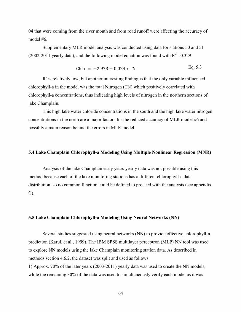
64

04 that were coming from the river mouth and from road runoff were affecting the accuracy of

model #6.

Supplementary MLR model analysis was conducted using data for stations 50 and 51

(2002-2011 yearly data), and the following model equation was found with R2= 0.329

Eq. 5.3

R2 is relatively low, but another interesting finding is that the only variable influenced

chlorophyll-a in the model was the total Nitrogen (TN) which positively correlated with

chlorophyll-a concentrations, thus indicating high levels of nitrogen in the northern sections of

lake Champlain.

This high lake water chloride concentrations in the south and the high lake water nitrogen

concentrations in the north are a major factors for the reduced accuracy of MLR model #6 and

possibly a main reason behind the errors in MLR model.

5.4 Lake Champlain Chlorophyll-a Modeling Using Multiple Nonlinear Regression (MNR)

Analysis of the lake Champlain early years yearly data was not possible using this

method because each of the lake monitoring stations has a different chlorophyll-a data

distribution, so no common function could be defined to proceed with the analysis (see appendix

C).

5.5 Lake Champlain Chlorophyll-a Modeling Using Neural Networks (NN)

Several studies suggested using neural networks (NN) to provide effective chlorophyll-a

prediction (Karul, et al., 1999). The IBM SPSS multilayer perceptron (MLP) NN tool was used

to explore NN models using the lake Champlain monitoring station data. As described in

methods section 4.6.2, the dataset was split and used as follows:

1) Approx. 70% of the later years (2003-2011) yearly data was used to create the NN models,

while the remaining 30% of the data was used to simultaneously verify each model as it was

65

created. After reviewing the literature, I found that most references suggest that for large

amounts of data, the data should be split 50% for training the models and 50% for verification of

the models. The literature also suggested that for handling smaller amounts of data, splitting it

70% for training models and 30% for verification models was best (Oded et al., 2008)

2) The results of the NN model analysis of the lake Champlain water quality monitoring data are

shown in Figures 5.5 and 5.6. Coefficient of determination for NN model #8 is R2= 0.851.

3) Early years (1992-2002) yearly data was used to verify NN model #8.

NN importance chart (figure 5.5, top panel) is a measure of how much the network’s

model-predicted value changes for different values of the independent variable; and this value is

divided by the largest value present them as a percentage. The results of the analysis showed that

the independent variable total phosphorus (TP) had the greatest effect on how the network

classifies chlorophyll-a models, followed by the variables secchi depth (Secchi; relative

importance (ri =40%), chloride (Cl; ri=20%) and total nitrogen (TN; ri=20%). Interestingly, the

NN analysis suggested that RegAlk was also important (ri=30%). The remaining variables tested

were considered relatively unimportant (ri <20% ). These results agree with the earlier MLR

modeling study (section 5.3) and also agree with the correlation analysis (section 5.1). They also

do agree with the published literature (Karul et al., 1999).

A plot of the observed Chla data verses NN model predicted Chla values are shown in

figure 5.5 (bottom panel). It can be seen that the error in prediction using NN model #8 is low for

low to moderate Chla levels (<10 μg/L) and the prediction becomes less accurate at higher Chla

levels (>10 μg/L). This is in good agreement with the MLR modeling study results (MLR model

#6, section 5.3)

66

Figure 5.5 NN analysis water quality variables importance chart (top panel) and Chla observed

values vs. NN model #8 predicted values for Chla in μg/L (bottom panel).

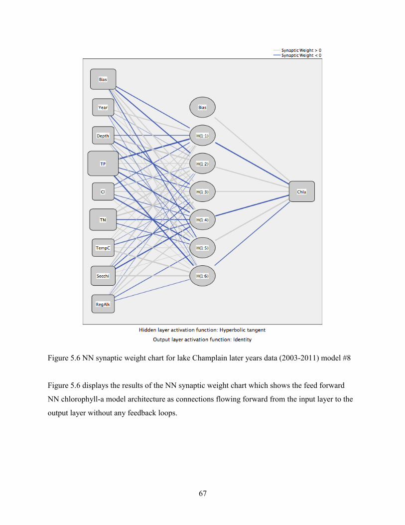
67

Figure 5.6 NN synaptic weight chart for lake Champlain later years data (2003-2011) model #8

Figure 5.6 displays the results of the NN synaptic weight chart which shows the feed forward

NN chlorophyll-a model architecture as connections flowing forward from the input layer to the

output layer without any feedback loops.

68

Fig

ure

5.7

Lak

e C

ham

pla

in c

hlo

rophyll

-a l

evel

s b

y y

ears

(2003

-2011),

NN

model

R2=

0.8

51

Obse

rved

lak

e C

ham

pla

in m

onit

ori

ng d

ata

(Chla

, gre

en l

ine)

, co

mpar

ed t

o p

redic

tions

gen

erat

ed u

sing t

wo c

hlo

rophyll

a

model

s (M

LR

model

#6 (

blu

e li

ne)

and N

N m

odel

#8 (

bla

ck l

ine)

, usi

ng t

he

sam

e dat

aset

s

69

5.5.1 NN model #8 verification

To verify NN model #8 (R2=0.851), which was created using the lake Champlain

monitoring station later years variable data (2003-2011)(see section 5.5), the model was tested

with variable data from lake Champlain early years (1992-2002). NN model #8 results were

compared with: 1) the actual observed results (Chla); and, 2) MLR model #6 results (section 5.3)

as shown in figure 5.8

.

Although the NN model #8 verification for the years between 1992-2002 resulted in

(R2=0.795) which is lower than verification of the MLR model #6 (R

2= 0.812) for the same

period, however it produced a better fit since the average absolute error between the NN model

#8 curve and the observed Chla data curve is less than 1.33, while for MLR model #6 the

average absolute error between the MLR model #6 curve and the observed Chla data curve was

2.19, this can also be noticed on prediction results of figure 5.8

It should be noted that running the same data set using NN model #8 will result in a

different NN model and result for each run, and this is due to the fact that NN is a learning

algorithm that works by minimizing the error successively from the previous equation.

Improving the NN results is an iterative and time-consuming process. Previous studies suggested

manipulating the number of layers and the ratio between the training and prediction data. I have

already implemented many of the recommended techniques to improve the prediction of the NN

model, but since NN does not produce any modeling equation, I decided to present only the best

model (model #8) that I found from the NN analysis.

70

Fig

ure

5.8

Lak

e C

ham

pla

in c

hlo

rophyll

-a l

evel

s b

y y

ears

(1992

-2002),

NN

model

R2=

0.7

95

Obse

rved

lak

e C

ham

pla

in m

onit

ori

ng d

ata

(Chla

, gre

en l

ine)

, co

mpar

ed t

o p

redic

tions

gen

erat

ed u

sing t

wo c

hlo

rophyll

a m

odel

s (M

LR

model

#6 (

blu

e li

ne)

and N

N m

odel

#8 (

bla

ck l

ine)

, usi

ng t

he

sam

e dat

aset

s

71

5.6 Lake Champlain Chlorophyll-a Modeling Using Data Mining (DM)

EUREQA DM software was used to analyze the lake Champlain total yearly dataset for

all years (early years + late years: 1992-2011) and produced several models. The complete

analysis is presented in appendix D. The best model found was arbitrarily named DM model #1

(figure 5.9) with a high goodness of fit (R2= 0.815), and is detailed in table 5.6.

5.6.1 DM modeling and water quality variables

Table 5.6 (left panel) shows the equation for DM model #1 which was produced after the

Eureqa DM software screened the lake Champlain total yearly dataset (1992-2011), which

included all the seven water quality variables listed in Table 4.1. It was found that the following

variables were the most significant and relevant variables for modeling and that these were

related in a complex manner: total phosphorus (TP), secchi depth (water clarity), and total

nitrogen (TN). This is in agreement with MLR model #6 results (section 5.3) and NN model #8

results (section 5.5).

DM model equation was nonlinear and the scatters plot for DM model #1 (table 5.6

indicates a uniform and small error distribution, which indicates the high accuracy of this model).

Chla =4.836 + 2.633*10-7

* TP * Secchi *TN2 + 2.63347*10

-7*

TP *TN2*COS(0.0663525 + Year) - 0.75498* Secchi

R2 Goodness of Fit = 0.815

Correlation Coefficient =0.902

Maximum Error=11.730

Mean Squared Error=4.200364

Table 5.6 Results of lake Champlain DM model #1 for (1992-2011)

72

5.6.2 Lake Champlain DM model #1 verification and comparison with MLR model #6 and

NN model #8

The DM modeling equations should be among the best to provide an accurate prediction

of lake Champlain chlorophyll-a levels, because the verification process immediately starts after

each model is created. To confirm this, all three lake Champlain chlorophyll-a models (MLR

model #6, NN model #8, and DM model #1) were compared with each other and with the

observed data (see figure 5.9). For this study, the following variables and input datasets were

used for the models detailed below.

1) Chlorophyll a MLR model #6 (R2 = 0.857) was generated using lake Champlain later years

(2003-2011) yearly dataset, which consisted of 50% of the total data, with 7 input variables,

while the verification of Chlorophyll a MLR model #6 for the early year (1992-2002) resulted in

(R2= 0.812)

2) Chlorophyll a NN model #8 (R2=0.851) was generated using lake Champlain later years

(2003-2011) yearly dataset. This model was created using 70% of the data, while 30% of the data

was used to verify the model, with 7 input variables, while the verification of Chlorophyll a NN

model #8 for the early year (1992-2002) resulted in (R2= 0.795)

3) Chlorophyll a DM model #1 (R2= 0.815) was generated using the lake Champlain total years

early data set, which consisted of 50% randomly chosen values from the dataset (years 1992-

2011) and the other 50% of this dataset was used to verify the model results, with 7 input

variables, however the verification of Chlorophyll a DM model #1 for the early year (1992-2002)

resulted in (R2= 0.786)

The results of this comparison indicated that NN model #8 predictions were more

accurate than both MLR model #6 and DM model #1 predictions, by 48% and 12.8%,

respectively, this results was obtained by comparing the errors resulted from the each model

prediction with the actual observed data between the years of 1992-2002, furthermore all the

three models are plotted against each other and against the observed Chlorophyll a data for the

entire study period between 1992-2011 in figure 5.9

73

Fig

ure

5.9

Obse

rved

lak

e C

ham

pla

in m

onit

ori

ng d

ata

1992

-2003 (

Chla

, gre

en l

ine)

com

par

ed t

o p

redic

tions

gen

erat

ed u

sing

thre

e ch

loro

phyll

-a m

odel

s (M

LR

model

#6 (

blu

e li

ne)

, N

N m

odel

#8 (

bla

ck l

ine)

and D

M m

odel

#1

(re

d l

ine)

, usi

ng t

he

dat

aset

s, v

aria

ble

s, a

nd o

utl

ier

condit

ions

des

crib

ed i

n t

he

text.

74

5.6.3 Comparison of chlorophyll-a DM, NN, MLR models with actual observations

At the beginning of writing this thesis, the lake Champlain data was only available till

2011, and recently in 2014 the data for the years of 2012 and 2013 were added, provided the

ability to test and verify the different models that I developed for this lake using the 2012-2013

data (see figure 5.10).

We notice from figures 5.10, 5.11 and 5.12 that NN model #8 predicted results for

chlorophyll-a levels were closer to the observed data than those of the other models tested,

including MLR model #6 and DM model #1 using recent data for years 2012-2013. Mean

absolute errors for MLR, NN and DM models were respectively 0.075, 0.053 and 0.068.

75

Fig

ure

5.1

0 O

bse

rved

lak

e C

ham

pla

in m

onit

ori

ng d

ata

(2012 a

nd 2

013

) co

mpar

ed t

o p

redic

tions

fro

m M

LR

model

76

Fig

ure

5.1

1 O

bse

rved

lak

e C

ham

pla

in m

onit

ori

ng d

ata

(2012 a

nd 2

013

) co

mpar

ed t

o p

redic

tions

fro

m N

N m

odel

77

Fig

ure

5.1

2 O

bse

rved

lak

e C

ham

pla

in m

onit

ori

ng d

ata

(2012 a

nd 2

013

) co

mpar

ed t

o p

redic

tions

fro

m D

M m

odel

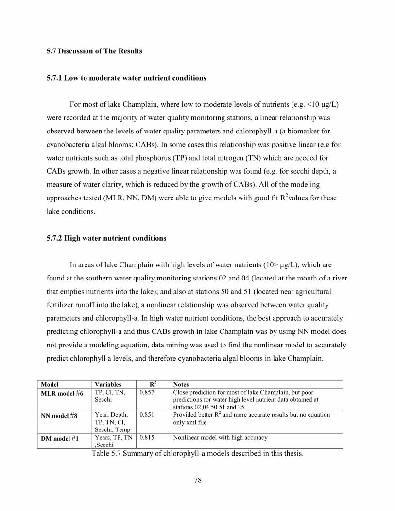
78

5.7 Discussion of The Results

5.7.1 Low to moderate water nutrient conditions

For most of lake Champlain, where low to moderate levels of nutrients (e.g. <10 μg/L)

were recorded at the majority of water quality monitoring stations, a linear relationship was

observed between the levels of water quality parameters and chlorophyll-a (a biomarker for

cyanobacteria algal blooms; CABs). In some cases this relationship was positive linear (e.g for

water nutrients such as total phosphorus (TP) and total nitrogen (TN) which are needed for

CABs growth. In other cases a negative linear relationship was found (e.g. for secchi depth, a

measure of water clarity, which is reduced by the growth of CABs). All of the modeling

approaches tested (MLR, NN, DM) were able to give models with good fit R2values for these

lake conditions.

5.7.2 High water nutrient conditions

In areas of lake Champlain with high levels of water nutrients (10> μg/L), which are

found at the southern water quality monitoring stations 02 and 04 (located at the mouth of a river

that empties nutrients into the lake); and also at stations 50 and 51 (located near agricultural

fertilizer runoff into the lake), a nonlinear relationship was observed between water quality

parameters and chlorophyll-a. In high water nutrient conditions, the best approach to accurately

predicting chlorophyll-a and thus CABs growth in lake Champlain was by using NN model does

not provide a modeling equation, data mining was used to find the nonlinear model to accurately

predict chlorophyll a levels, and therefore cyanobacteria algal blooms in lake Champlain.

Model Variables R2 Notes

MLR model #6 TP, Cl, TN,

Secchi

0.857 Close prediction for most of lake Champlain, but poor

predictions for water high level nutrient data obtained at

stations 02,04 50 51 and 25

NN model #8

Year, Depth,

TP, TN, Cl,

Secchi, Temp

0.851 Provided better R2 and more accurate results but no equation

only xml file

DM model #1 Years, TP, TN

,Secchi

0.815 Nonlinear model with high accuracy

Table 5.7 Summary of chlorophyll-a models described in this thesis.

79

5.7.3 Causes of the model errors

Investigation of the models errors revealed that:

The errors in MLR model were due to:

a. High correlation between the lake input variables (Diebold et al., 2007).

b. Chla general distribution is nonlinear, which was proven in appendix C, and it

was observed from the data mining that Chla model in general is not linear, so it

is likely that linear regression was not able to fully address the nonlinear part of

the lake data.

c. The model most significant errors were for the northern as southern parts of the

lake and were due to the extreme concentrations of Chloride (Cl) in the southern

part of the lake, and extreme concentrations of nitrogen (TN) in the northern part

of the lake.

NN model provided better accuracy than the MLR; the main cause of errors in the model

was due to the extreme concentrations of Chloride (Cl) in the southern part of the lake, and

extreme concentrations of nitrogen (TN) in the northern part of the lake.

DM model was more responsive to extreme changes as it used complicated algorithms to

derive the DM model, and similar to NN model the DM model main cause of errors were due to

the extreme concentrations of Chloride (Cl) in the southern part of the lake, and extreme

concentrations of nitrogen (TN) in the northern part of the lake.

Further investigation of the data generated by the lake Champlain water quality

monitoring stations that were causing problems in model prediction accuracy revealed that, the

southern monitoring stations 02 and 04 are located in shallow water at the mouth of the Poultney

river that contributes large amount of nutrients into the lake. Furthermore, farms and agricultural

lands that likely contribute fertilizer into the lake surround the northern monitoring stations 50

and 51. The results obtained in this thesis project have been confirmed by other studies in the

literature, which showed that the MLR model approach is not accurate at high water nutrient

concentrations (Li et al., 2013).

Results of model comparison indicated that NN model #8 predictions were more accurate

than both MLR model #6 and DM model #1 predictions, by 48% and 12.8%, respectively.

80

CHAPTER 6

LAKE CHAMPLAIN

CHLOROPHYLL-A GIS SPATIAL ANALYSIS

RESULTS

81

In the previous chapter using statistical analysis we revealed several chlorophyll-a

models for lake Champlain. The best model comprised a set of 3 different equations found

through data mining. One model was for the southern part of the lake, another for the northern

and a final set for the main lake body. Such distribution suggests that location might be a factor

in modeling algae in lake Champlain. In this chapter I’ll present geostatistical analysis to

investigate the location importance to the algae bloom in Lake Champlain and show the spread

of the different variables contributing to the algae model across the lake.

6.1 GIS Based Modeling Results

In the previous chapter, the variables contributing to chlorophyll-a models for lake

Champlain were identified through statistical analysis, and it was noted that the different models

found were less accurate at the northern and southern parts of the lake, further investigation

revealed that northern parts of the lake suffers from excess levels of nitrogen, while southern

parts of the lake suffers from excess levels of chloride, such phenomena suggests that the

location might be a factor in modeling algae in Lake Champlain, so in this section geostatistical

analysis is used to investigate the location impact on algae bloom for lake Champlain,

furthermore the geostatistical analysis will be used to mathematically interpolate the levels of

variables throughout the volume of the lake.

6.2 Determination of the Statistical Model Variables

The purpose of this test is to determine the location importance to the MLR chlorophyll-a

model. ArcGIS is advanced geostatistical analysis software, however it lacks the stepwise

selection option available in IBM SPSS, therefore in the MLR variables test, all of the variables

for lake Champlain water quality parameters were used. The data for later years 2003-2011 was

used to generate the model equation, while the early years data 1992-2002 was used to verify the

model results. The processing extent and snap raster of the analysis were set to the lake

Champlain boundary. Figure 6.1 shows the GIS ordinary least square (OLS) setup interface.

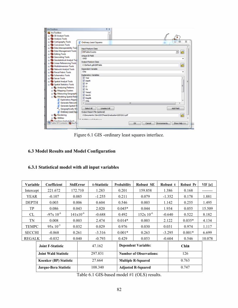
82

Figure 6.1 GIS -ordinary least squares interface.

6.3 Model Results and Model Configuration

6.3.1 Statistical model with all input variables

Variable Coefficient StdError t-Statistic Probability Robust_SE Robust_t Robust_Pr VIF [c]

Intercept 221.672 172.710 1.283 0.201 159.858 1.386 0.168 --------

YEAR -0.107 0.085 -1.255 0.211 0.079 -1.352 0.178 1.881

DEPTH 0.003 0.006 0.604 0.546 0.003 1.142 0.255 1.495

TP 0.086 0.043 2.020 0.045* 0.044 1.934 0.055 15.509

CL -97x 10-6

141x10-6

-0.688 0.492 152x 10-6

-0.640 0.522 8.182

TN 0.008 0.003 2.474 0.014* 0.003 2.122 0.035* 4.134

TEMPC 95x 10-5

0.032 0.029 0.976 0.030 0.031 0.974 1.117

SECCHI -0.868 0.261 -3.316 0.001* 0.263 -3.295 0.001* 6.699

REGALK -0.032 0.040 -0.793 0.429 0.053 -0.604 0.546 10.078

Joint F-Statistic 47.162 Dependent Variable: Chla

Joint Wald Statistic 297.831 Number of Observations: 126

Koenker (BP) Statistic 27.664 Multiple R-Squared 0.763

Jarque-Bera Statistic 108.340 Adjusted R-Squared 0.747

Table 6.1 GIS-based model #1 (OLS) results.

83

From table 6.1, we notice that the Koenker test value is >0.05. This means that the

geographical location of the water quality parameters (variables) may not have a significant

impact on the GIS based model. However, the MLR model obtained in this step was not the

optimal solution, since there were several variables with VIF >7.5, indicating that some variables

might be redundant (dismissible).

6.3.2 Statistical model with selected variables

Previously, we found through use of correlation analysis, that lake Champlain variables

were strongly correlated, thus removing the variables with VIF>7.5 may not be the best approach

(e.g. total phosphorus (TP) and total nitrogen (TN), particularly at high levels). Therefore several

iterations are required to find the best set of input of variables that produce the optimal MLR

model, or we can use the set of input variables obtained from the MLR model stepwise selection

since we already know they produced the optimal MLR model. GIS based model (OLS) run

results are presented in the following table.

Variable Coefficient Std Error t-Statistic Probability Robust_SE Robust_t Robust_Pr VIF [c]

Intercept 4.131 1.874 2.204 0.029* 2.297 1.798 0.074 --------

TP 0.070 0.030 2.331 0.0213 0.034 2.004 0.047* 6.591

CL - 0.00015 0.000056 - 2.651 0.009* 0.00007 -2.123 0.035* 1.290

TN 0.010 0.002 4.101 0.00008* 0.003 3.460 0.0007** 2.733

SECCHI - 0.701 0.2343 -2.994 0.003* 0.232 -3.024 0.003* 5.369

Joint F-Statistic 93.493 Dependent Variable: CHLa

Joint Wald Statistic 241.618 Number of Observations: 126

Koenker (BP) Statistic 25.555 Multiple R-Squared 0.857

Jarque-Bera Statistic 73.763 Adjusted R-Squared 0.854

Table 6.2 GIS- based model# 2 (OLS) results

The set of input variables used for this run resulted in all of the variables having their VIF

<7.5, thus confirming that we chose the right set of variables which were significant for this

model. The Koenker test value was >0.05, indicating the insignificance of the geographical

location impact on the algae model. Furthermore, the JarqueBera statistic of > 0.05 indicates the

84

residuals (errors) are normally distributed and the model is well distributed and not biased. The

other outputs from the OLS test, (e.g. the robust probabilities, Robust_SE, Robust_t, Joint Wald

Statistic and Joint F-Statistic), all became insignificant, as we only considered their value when

the Koenker Statistic was< 0.05.The equation from OLS model with the selected input variables

is:

Eq. 6.1

With R2= 0.857

Recall equation 5.1 using IBM SPSS MLR stepwise selection.

Eq. 5.1

The two equations are identical; this result was expected because when the location has

no impact on the chlorophyll-a model, then ArcGIS produces similar results to those obtained by

statistical analysis tools like IMB SPSS, or Systat 13. This finding suggests that high/low levels

of chlorophyll-a and thus cyanobacteria algal blooms (CABs) could occur anywhere throughout

lake Champlain, depending on the seasons and natural and man-made environmental conditions

(e.g. presence of farm fertilizer runoff into the lake in some years but not in others and prevailing

wind/currents in the lake that distribute the phosphorus and nitrogen throughout the lake).

6.4 Spatial Trend Analysis

Spatial analysis is also required to show the spread, distribution and extent of the

variables affecting the chlorophyll-a model for cyanobacterial algal bloom growth. ArcGIS uses

the interpolation technique Empirical Bayesian Kriging to create a continuous surface, a method

well suited to handle extreme and minor changes within data records. Using Kriging, the

surrounding measured values are weighted to derive a predicted value for an unmeasured

location. Weights are based on: the distance between the measured points, the prediction

locations and the overall spatial arrangement among the measured points. The Empirical

Bayesian Kriging (EBK) tool is available in ArcGIS to automate calculation of the interpolated

surface for the various water quality input parameters, generating maps that represent the

distribution of the variable over the entire lake volume and surface.

85

In the EBK interface input menu, the water quality parameters (phosphorus, nitrogen,

chloride, secchi depth, alkalinity and chlorophyll-a) that we wish to interpolate and have their

values projected on a map throughout the lake are added one by one. The EBK surface output is

stored in the Z value field from EBK interface menu. In the environment settings, the processing

extent and the snap raster are set to be the lake Champlain boundary and in the layer properties

the clip options are set to lake Champlain layer, the last step is necessary to limit the analysis to

the lake boundary.

Figure 6.2 GIS Kriging inputs.

Figure 6.3 shows a summary of the total phosphorus (TP) levels obtained from the water

quality monitoring stations in lake Champlain from years 1992 to 2011, illustrated in an

interpolated (EBK) map. This figure shows the normal seasonal and yearly variations in the lake

phosphorus levels, which are generally lower in the center of the lake (blue colour) and higher in

the Northern and Southern sections of the lake (red colour), likely due to farm fertilizer runoff

(in the North) and the rivers (in the South). The addition of a water quality monitoring station 51

in 2005 confirmed the high phosphorus levels previously observed at monitoring station 50 in the

Northern section of the lake (red colour).

86

Figure 6.4 and 6.5 for the EBK map which clearly highlights the problem causing the

deviated results in the models predictions, as we can see extreme concentrations of chloride (Cl)

in the southern part of the lake, thus confirming the analysis in section 5.3 and the MLR model

equation 5.2, similarly we can see extreme concentrations of total nitrogen (TN) in the northern

part of the lake, thus confirming the analysis in section 5.3 and the MLR model equation 5.3.

This is rendering the two sections (the northern and southern) parts of the lake as different

extreme environment.

Figure 6.6 shows the results for secchi depth monitoring in lake Champlain between

1992-2011, the EBK maps for the secchi depth confirm the correlation analysis in section 5.1

and MLR model #6 and equation 5.1 as well as the data mining modeling equation 5.4, as we

notice that secchi depth which is a measure of the water clarity is reduced by increasing levels of

cyanobacterial algal bloom (CABs) growth

Figure 6.7 shows a different trend for alkalinity monitoring in lake Champlain between

1992-2011. Alkalinity is the ability of a solution to neutralize acids. Alkalinity levels are subject

to minor changes through the years thus it seems that the CABs growth in lake Champlain is not

being affected by alkalinity, and this is supported by the analysis in chapter 5 as none of the

modeling equations contain the alkalinity as a predictor.

87

Figure 6.3 GIS map showing a summary of lake Champlain total phosphorus (TP) levels

monitored at various stations throughout the lake from 1992-2011.

88

Figure 6.4 GIS map showing a summary of lake Champlain total nitrogen (TN) levels monitored

at various stations throughout the lake from 1992-2011.

89

Figure 6.5 GIS map showing a summary of lake Champlain chloride (Cl) levels monitored at

various stations throughout the lake from 1992-2011.

90

Figure 6.6 GIS map showing a summary of lake Champlain secchi depths (a measure of water

clarity) monitored at various stations throughout the lake from 1992-2011.

91

Figure 6.7 GIS map showing a summary of lake Champlain alkalinity levels (an inverse measure

of water acidity) monitored at various stations throughout the lake from 1992-2011.

92

6.5 GIS Based Statistical Model Validation and GIS Results for TP and Chla

In section 6.4 the interpolated EBK maps of lake Champlain water quality monitoring

data were used to show the trend for the variables appearing in the cyanobacterial algal bloom

(CABs) model, and the EBK maps came to confirm the results of the different models,

furthermore for better visualization for the results presented for the MLR in figure 6.8 we can

use the EBK maps to present the cyanobacterial algal bloom spread side by side by the main

factors contributing in the MRL cyanobacteria model thus helping to better understand and

verify the model.

Figure 6.8 presents a pair of maps for the observed chlorophyll-a (Chla) side by side by

the Total Phosphorus (TP) which was found to be the most dominant factor affecting

cyanobacterial algal bloom (CAB) according to the multiple linear regression, neural network

and data mining models, where we can clearly see the similarity between the TP and Chla spread

of concentrations throughout the years of lake Champlain, thus verifying the results obtained by

the multiple linear regression, neural network and data mining models

Figure 6.9 and 6.10 respectively present a pair of maps showing the prediction results

from the GIS (OLS) model #2 output verses the observed recorded values. We can see that the

chlorophyll-a GIS (OLS) model #2 results, were accurate and consistent in the main lake body

and the accuracy tends to drop in the northern and southern parts of the lake for the reason

discussed earlier in this chapters.

93

Fig

ure

6.8

GIS

map

s co

mpar

ing l

ake

Cham

pla

in c

hlo

rophyll

-a o

bse

rved

lev

els

wit

h t

ota

l phosp

horu

s (T

P)

obse

rved

lev

els

bet

wee

n

2004

-2011.

94

Figure 6.9 Lake Champlain water quality monitoring station observed chlorophyll-a levels (Chla

a biomarker for CABs) compared to the GIS model #2 predicted levels.

95

Fig

ure

6.1

0 L

ake

Cham

pla

in m

onit

ori

ng s

tati

on o

bse

rved

chlo

rophyll

-a l

evel

s vs.

the

ML

R m

odel

#6 p

redic

ted l

evel

s.

96

CHAPTER 7

CONCLUSION AND CONTRIBUTION

97

7.1 Conclusion

This study provided information, data and an overview of research on modeling of the

factors affecting cyanobacterial algal bloom as well as my subjective opinions related to the

factors affecting the water quality in lake Champlain.

A statistical analysis and simulation models including: (a) multiple linear regressions

(MLR); (b) artificial neural network (ANN) based on back propagation algorithms; (c) data

mining (DM) were developed using multiple water quality parameters such as the total

phosphorus, total nitrogen, temperature, water monitoring depth, water clarity as an input while

using the chlorophyll-a levels which is a biomarker for algal growth as an output to these models.

A GIS modeling structure of lake eutrophication was developed to support the statistical analysis.

The results of the statistical analysis indicate that neural network model had the most accurate

predictions followed by data mining, then the multiple linear regression and that's due to the fact

that Chla growth is nonlinear. The developed chlorophyll-a models showed various degrees of

accuracy in predicting chlorophyll-a levels, the results of the MLR in particular are less accurate

due to the high correlation between the input variables, and the nonlinear characteristics of

Chlorophyll-a at high levels of lake variables ,while in NN and data mining the errors were not

random, they came from stations 02, 04, 50 and 51.The analysis indicates that excessive levels of

Chloride at the southern section of lake Champlain and excessive levels of Nitrogen at the

northern section of the lake were the two factors affecting the NN and data mining chlorophyll-a

model accuracy.

The water quality parameter (variable) found to be most significantly correlated with

chlorophyll-a levels was total phosphorus (TP). The phosphorus cycle in lake Champlain shows

that there are many natural and human sources of phosphorus in the lake, including the mouth of

a river bringing phosphorus-rich sediment into the southern section of the lake, and farms with

fertilizer runoff located at the northern part of the lake. This suggests that the natural

environment as well as human activity contribute perhaps equally to lake eutrophication and

algae blooms. The natural and man made high levels of phosphorus and other nutrients such as

nitrogen promoting algal growth and controlling these levels are the key issue related to

minimizing the probability of algal blooms.

98

The geostatistical analysis indicated that hi/low levels of chlorophyll-a and thus

cyanobacterial algal blooms (CABs) could occur anywhere throughout lake Champlain, and it is

independent of the location.

The investigation of the different lake Champlain timeframes, suggests that: smaller

timeframes such as daily and weekly, doesn’t not support developing a significant model; and

since the significant models came from the yearly timeframes, then it means that the developed

model can’t be used as an early alert for increasing levels of algae or eutrophication but rather as

a tool to help developed proper lake management programs.

7.2 Contributions of the Research

As the regulations are being developed and enforced to protect and improve water quality

in lakes, rivers and reservoirs, understanding algal blooms (using the biomarker chlorophyll-a) is

becoming more and more important. In the present thesis study, several analytical techniques

were used to uncover the water quality parameters that are correlated with algal bloom. Several

models for chlorophyll-a were developed, and for these different models, the degree to which

each environmental variable contributed to chlorophyll-a levels varied. Taken together, the set of

different chlorophyll-a models that were developed using different approaches (e.g. multiple

linear regression (MLR), neural network (NN), and data mining (DM), all indicated a strong

linear relationship between the dissolved total phosphorus (TP) levels and chlorophyll-a levels in

the lake water, most likely because phosphorus is an important nutrient for algal growth. This

relationship was found to be linear at low to medium concentrations of TP. However, at high

concentrations of total phosphorus (>10 μg/L), the relationship became nonlinear.

The contributions of the present thesis can be summarized as follows:

1) Analysis of lake Champlain data indicates that using the mean values of the data (yearly) have

had refined to a relatively high degree of statistical precision and to create the models.

The later years dataset worked better as a training data set. This was because several new

important monitoring stations were set up during the later years time period.

99

2) Although MLR model had the highest value, however the model produced the least

accurate predictions. The deviation in the model accuracy was due to 1) high correlation between

the environmental variables. 2) extreme levels of nitrogen in north and chloride in the south. 3)

Chlorophyll-a has nonlinear characteristics at high levels of lake variables. 4) and in section

4.5.C I ignored the impact of internal loading which in this case should be considered as those

are shallow stations with lots of sediment interaction .The best predictions came through NN

model, however NN model did not provide a model equation to help future researchers

investigation, the alternative came through data mining, which provided a significant accurate

model with an equation that can be used to further investigate the lake on future studies.

3) Model verifications indicated less accurate results for the northern and southern parts of the

lake, further investigation supported by Empirical Bayesian Kriging (EBK) maps highlighted the

cause of the problem to be due to the extreme concentrations of chloride (Cl) in the southern part

of the lake, and extreme concentrations of total nitrogen (TN) in the northern part of the lake.

4) Modeling studies in this thesis for chlorophyll-a indicate that: the total dissolved phosphorus

has the strongest impact on algae production and the main cause to water quality degradation due

to its persistence in lake water at high levels.

5) Earlier studies for lake Champlain haven’t produced a good prediction equation (Smeltzer et

al., 2009); this study is one of the first to produce several modeling equations with high

prediction accuracy to address the algal problem in lake Champlain. The developed chlorophyll-

a models showed various degrees of accuracy in predicting chlorophyll-a levels therefore, it is ill

advised to assume that one model can account for all the variations in the chlorophyll-a equation.

Furthermore, we cannot generalize the use of any of these models for other lakes because each

lake will respond differently to its environment.

In general, this study helped to identify the water quality factors that most significantly affect

chlorophyll-a levels (correlated with cyanobacterial algal bloom growth) in lake Champlain.

Although the models developed for the case study may not apply for a different lake, the factors

affecting the algal blooms may be similar for all lakes.

100

7.3 Future Studies

This section highlights the scope of future work, which may be conducted on the basis of

the work presented in this thesis.

1. Lake recovery from eutrophication depends in part on the quantity of phosphorus that has

accumulated over time in the lake bottom sediment and in the quantity of dissolved

phosphorus in the water volume in contact with the sediment. Reduction of external

phosphorus loading may not necessarily produce swift improvement, since sediment

release can compensate for this reduction, consequently, both internal and external

loading data reduction should be considered in preparing a proper lake management

program.

2. It was not possible to utilize multiple nonlinear regression due to the inconsistency of the

monitored data, however with the aid of new technology such as GIS analysis we were

able to expose the hidden information patterns and the problems in the north and south

parts of the lake. The scientific works published on GIS lake eutrophication models are

still very limited. Further and deeper scientific research should be conducted in this area

in the future.

3. The comprehensive statistical analysis exposed that the northern and southern parts of the

lake have complicated and uncertain patterns, and were ill defined using multiple linear

regression, therefore for future studies fuzzy and/or stochastic modeling methods can be

used to further address uncertainties.

4. ArcGIS in comparison to other professional statistical analysis software like IBM SPSS

or data mining has limited capabilities and has less accuracy. Future studies should try to

import models developed outside GIS and import and implement those models into the

GIS for enhanced and improved predictions.

5. The goal of any monitoring plan is to be able to take action before the problem becomes

uncontrollable. Huge efforts were made in collecting lake Champlain water quality

monitoring data, however, the daily data for lake Champlain did not help much in

101

producing any of the chlorophyll-a models. lake Champlain data would also have been

much more valuable if it was collected concurrently.

6. During the modeling process, I assumed that all the lake variables are independent

however, this is not the case in fact most of the variables are correlated with the climate

conditions, so climate impact on lake water quality is a subject for further investigation.

7. The developed models can be further used to find an effective methodology for lake

Champlain management, and suggest programs/regulations, which can help improve the

lake water quality.

102

REFERENCES

103

REFERENCES

Aaby, A.A. (2005). Thesis Testing the ArcGIS Marine Data Model: Using Spatial Information to

Examine Habitat Utilization Patterns of Reef Fish along the West Coast of Hawaii. Oregon

State University

Akdeniz, S., Karaer, F., Katip, A., and Aksoy, E. (2011). A GIS-Based Method for Shallow Lake

Eutrophication Assessment. Journal of Biological and Environmental Sciences, 5(15): 195-

202

Aleksandar, O., Topuzoviić, M., and Stefanović, D. (2012). Management Information System of

Lakes and Reservoirs. Water Resources, 39(4): 488-495.

Anoh, J., and Kouamé, K.L. (2012). Demarcation of Protection Perimeters for the Surface

Waters of Taabo (Ivory Coast) Watershed Using GIS and Multicriteria Analysis.

Environmental Engineering and Management Journal, 11(12): 123-2131.

Arheimer, L. (2000). Nitrogen and Phosphorus Concentrations from Agricultural Catchments-

Influence of Spatial and Temporal Variables. Journal of Hydrology, 227: 140-159.

Allison, P.D. (1998). Allison Multiple Regression: A Primer (Research Methods and

Statistics)(1st edition). Pine Forge Press. California, USA.

Bailey, K. (1994). Numerical Taxonomy and Cluster Analysis. Typologies and Taxonomies.

Sage Publication Incorporation. Oka, California, USA, 102: 31-45.

Bishop, C. (2006). Pattern Recognition and Machine Learning (2nd edition). Springer Science

Media. New York, USA.

Bostrom, A.F., and Jansson, K. (1988). Exchange of Phosphorous across the Sediment-Water

Interface. Hydrobiologia, 170: 229-244.

Bostrom, B. (1984). Potential Mobility of Phosphorus in Different Types of Lake Sediment.

Gesamten Hydrobiologia, 69: 457-474.

Brewka, G. (1991). Nonmonotonic Reasoning: Logical Foundations of Commonsense.

Cambridge University Press. Acm Suigart Bulletin, 3(2): 28-29.

Brown, C., Canfield, D., Bachmann, R., and Hoyer, M. (1998). Seasonal Patterns of Chlorophyll,

Nutrient Concentrations and Secchi Disk Transparency in Florida Lakes. Lake and

Reservoir Management, 14(1): 60-76.

Canfield, D.C., Cooler, D.E., Haller, W.T., Watkins, C.E., and Maceina, M.J. (1984). Predictions

of Chlorophyll-a Concentrations in Florida Lakes: Importance of Aquatic Macrophytes.

Canadian Journal Fish Aquatic Science, 41: 409-501.

104

Chapra, S.C. (2008). Surface Water Modeling. (3rd edition). Waveland Press Incorporation.

Chicago,USA.

Chambers, P.A., Guy, M., Roberts, E.S., Roberts, M.N., Kent R., Gagnon ,C., and Grove, G.

(2001). Nutrients and their Impact on the Canadian Environment. Agriculture and Agri-

Food Canada, Environment Canada, Fisheries and Oceans Canada, Health Canada, and

Natural Resources Canada, Ottawa, Ontario, 239-241.

Chambers, J., William, C., Beat, K., and Paul, T. (1983). Graphical Methods for Data Analysis

(1st edition). Chapman and Hall/CRC. London.

Chen, Q., and Mynett, A.E. (2003). Integration of Data Mining Techniques and Heuristic

Knowledge in Fuzzy Logic Modeling of Eutrophication in Taihu Lake. Ecological

Modeling Journal, 162: 55-67.

Christopher, F., James, G., and Walter, R. (2011). Nutrient Enrichment Studies in a Coastal Plain

Estuary: Phytoplankton Growth in Large-Scale, Continuous Cultures. Canadian Journal of

Fisheries and Aquatic Sciences, 43(2): 397-406.

Correll, D.L. (1998). The Role of Phosphorus in the Eutrophication of Receiving Waters: A

Review Journal of Environmental Quality, 27: 261-266.

Cüneyt, K., and Soyupak, S. (1999). Neural Network Models as a Management Tool in Lakes.

Hydrobiologia, 408: 139-144.

Das, A., (2003). Thesis, Regional Water Quality Models for the Prediction of Eutrophication

Endpoints. University of Calcutta.

Di, M., and Jianhua. (2011). Eutrophication Assessment of a Large Scale Coastal Area Using

GIS Technologies. School of Environmental Science and Technology. Tiajin University,

China. Advanced Materials Research, 219: 1073-1076.

Diebold, F.X., (2001). Elements of Forecasting. University Pennsylvania, Ohio-South-Western.

Thomson Learning, (7): 249-271.

Dieter, M.I. (1973). Phosphorus Model of Lake Eutrophication. Swiss Federal Institute of Water

Resource and Water Pollution Control (EAWAG), (19): 297-204.

Dirk, C. (2007). GIS and Integrated Water Resource Management, Position IT– GIS Technical.

Paper Presented in GIMS User Conference Johannesburg.

Dixon, W.J. (1950). Analysis of Extreme Values, Annals of Mathematical Statistics. University

of Orefon, USA. Jstor journal, 21(4): 488-506.

105

Dodds, W.K., Bouska, W.W., Eitzmann, J.L., Pilger, T.J., Pitts, K.L., Riley, A.J., and Schloesser,

J.T. (2009). Eutrophication of U.S. Freshwaters: Analysis of Potential Economic Damages.

Environmental Science and Technology, 43: 1-2.

Dodds, W.K., Jeffrey, L., Tyler, J., Kristen, L., and Alyssa, J. (2009). Eutrophication of U.S.

Freshwaters-Analysis of Potential Economic Damages. Environmental Science and

Technology, 43(1): 12-19.

Douglas, C.M., Elizabeth, A., Peck, G., Geoffrey,V. (2012). Introduction to Linear Regression

Analysis (5th Edition). A John Wiley and Sons Publication. Hannover, Germany.

Dugdale, R.C. (1967). Nutrient Limitation in the Sea: Dynamics, Identification and Significance.

Limnol Oceanogr, 12: 685-95.

Downing, J.A., and McCauley, E. (1992). The Nitrogen Phosphorus Relationship in Lakes. The

American Society of Limnology and Oceanography, 37(5): 936-945.

Draper, N., and Smith, H. (1998). Applied Regression Analysis (3rd Edition). Wiley-Inter

Science Publication. New York, USA.

Eisenhauer, J.J. (2003). Regression Through the Origin. Teaching Statistics an International

Journal for Teacher, 25(3): 76-80.

Elwood, J.W., Newbold, J.D., and Van, W.W. (1980). An Operational Paradigm for Analyzing

Lotic Ecosystems. Oak Ridge National Lab. Conference: Stream Ecology Symposium,

Augusta. Georgia, USA, 19 Oct 1980.

Elwood, J.W., Newbold, J.D., Trimble, A.F., and Stark, R.W. (1983). The Limiting Role of

Phosphorus in a Woodland Stream ecosystem: Effects of P Enrichment on Leaf

Decomposition and Primary Producer. Ecology, 62: 146-158.

Environmental Systems Research Institute (Esri) (2006). Products- ArcGIS Desktop.

http://www.esri.com/software/arcgis/index.html. Accessed July 6, 2014

EPA. (2012). Cyanobacteria and Cyanotoxins: Information for Drinking Water Systems, EPA

Report http://water.epa.gov/scitech/swguidance/standards/criteria/nutrients Accessed

March 16, 2015

EPA. (2013). The Great Waters Program, Lake Champlain. Environment Protection Agency

(EPA) Report http://www.epa.gov/oaqps001/gr8water/xbrochure/champlai.html. Accessed

March 16, 2015

Eynard, F., Frédéric, E., Konstanze, M., and Jean, L.W. (2000). Risk of Cyanobacterial Toxins in

Riga Waters -Latvia. Water Research, 34 (11): 2979-2988.

106

Fluck, R.C., Fonyo, C., and Flaig, E. (1992). Land-Use-Based Phosphorus Balances for Lake

Okeechobee, Florida, Drainage Basins. Applied Engineering in Agriculture, 8: 813–820.

Froelich, P.N. (1988). Kinetic Control of Dissolved Phosphate in Natural Rivers and Estuaries: A

Primer on the Phosphate Mechanism. Journal of limnology and Oceanography, 33: 649-

668.

Gaddis, A., Erica, J.B., and Alexey, V. (2010). Spatially Explicit Modeling of Land Use Specific

Phosphorus Transport Pathways to Improve TMDL Load Estimates and Implementation

Planning. Water Resources Management, 24(8): 1621-644.

George, B., Song, S., Qianb, C.A., Stowc, E., Conrad, L., and Kenneth, H. (2007).

Eutrophication Risk Assessment using Bayesian Calibration of Process-Based Models:

Application to a Mesotrophic lake. Ecological Modeling Journal, 20: 215-229.

George, K., and Small, J.R. (2010). Introduction to Marine Biology (3rd edition). Cengage

Learning. Belmont, USA.

Goodwin, T.A., and White, C.E. (2011). Lithogeochemistry, Petrology, and Theacid-Generation

Potential of the Goldenville and Halifax Groups and Associated Granitoids Rocks in the

Metropolitan Halifax Regional Municipality.Nova Scotia, Canada. Atlantic Geology, 47:

158-184.

Goodwin, S.A. (2011). Thesis : Excess Nutrients and Cultural Eutrophication of the Cache la

Poudre River. Colorado State University.

Grobler, D.C., and Silberbauer, M.J. (1985). The Combined Effect of Geology, Phosphate

Sources and Runoff on Phosphate Export from Drainage Basins. Water Research Journal,

19 (8): 975-981.

Gruessner, B., William, G., Lescaze, M., and Stickney, M. (2003). Lake Champlain Basin

Management Experience Brief. Lake Champlain Basin Program #54 West Shore Road

Grand Isle, Vermont, USA.

Gupta, N., Aktaruzzaman, M., and Wang, C. (2011). GIS-Based Assessment and Management of

Rönneå River Catchment. Sweden. Indian Society of Remote Sensing Journal, 15(3): 217-

223.

Hameed, H.D., and Mesopot, J. (2010). GIS as a Tool for Classification Lake’s Acidification and

Eutrophication Degree. Mesopotamian Journal of Marine Science, 25 (1): 53-64

Handan, Ç., Nilsun, D., Arzu, K., and Sýddýk, K. (2005). Use of Principal Component Scores in

Multiple Linear Regression Models for Prediction of Chlorophyll-a in Reservoirs.

Department of Fisheries, Faculty of Agriculture, University of Ankara, Ankara. Turkey

Ecological Modeling. DOI: 10.1016/j.ecolmodel.2004.06.043

107

Hipp, J., Güntzer,U.,and Nakhaeizadeh,G. (2000). Algorithms for Association Rule Mining. A

General Survey and Comparison .Acm Sigkdd Explorations Newsletter, 2: 58-64.

Hirsch, R.M., Helsel., D.R, Cohn, T.A., and Gilroy, E.J. (1992). Statistical Analysis of

Hydrologic Data (3rd edition). McGraw-Hill. New York, USA.

Hiscock, J.G., Thourot, C.S., and Zhang, J. (2003). Phosphorous Budget–Land Use Relationships

for the Northern Lake Okeechobee Watershed Florida. Ecological Engineering Journal,

21(1): 74-12.

Horne, A.J., and Little, J.C. (1998). Lakes and Reservoirs. Management (1st edition). Elsevier

Incorporation. San Diego, USA.

Iyer, R., Menon, V., Buice, M., Koch, C., and Mihalas, S. (2013). The Influence of Synaptic

Weight Distribution on Neuronal Population Dynamics. Plos Computational Biology

Journal. DOI: 10.1371/journal.pcbi.1003248

Jan, T., Wu, S., Chou, P., Wen, C. (2005). Eutrophication Modeling of Reservoirs in Taiwan.

Science Direct Environmental Modeling and Software, 21(6): 829-844

Jie, C., Xinsheng, L., Zhihua, Z., and Hanting, Z. (2013). Eutrophication Assessment Based on

Set Pair Analysis –A Case Study in Sand Lake of Yinchuan Plain, China. Journal of

Environmental Science, Computer Science and Engineering and Technology, 2(3): 578-

585

John, M., Michael, K., Christopher, N., and William,W. (1996). Applied Linear Regression

Models. (3rd edition). McGraw Hill/Irwin Series. Boston, USA.

Jordan, T.E., Correll, D.L., and Weller, D.E. (1991). Long-Term Trends in Estuarine Nutrients

and Chlorophyll, and Short-Term Effects of Variation in Watershed Discharge. Marine

Ecology Progress Series, 75: 121-132.

Jordan, T.E., Correll, J., and Weller, D.E. (1997). Effects of Agriculture on Discharges of

Nutrients from Coastal Plain Watersheds of Chesapeake Bay. Journal of Environmental

Quality, 26: 836-848.

Jordan, T.E., Correll, J., and Weller, D.E. (1997). Nonpoint Source Discharges of Nutrients from

Piedmont Watersheds of Chesapeake Bay. Journal of the American Water Resources

Association, 33: 631-645.

Junsan, Z. (2009). GIS-Based Support Models for the Development of Erhai Lake Watershed

Management Information System. Geoscience and Remote Sensing Symposium, IEEE

International Journal, 2: 662-665.

108

Jeppesen. (2009). Climate Change Effects of Runoff, Catchment Phosphorus Loading and Lake

Ecological State, and Potential Adaptations. Journal of Environmental Quality. DOI:

10.2134/jeq2008.0113, 24(38): 5.

Jeong, K.S., Kim, D.K., Whigham, P., and Joo, G.J. (2003). Modeling Microcystis Aeruginosa

Bloom Dynamics in the Nakdong River by Means of Evolutionary Computation and

Statistical Approach. Ecological Modeling journal, 161: 67-78.

Luvalle, M.J., and Leon R.C. (1999). Kinetic Modeling of Hydrogen Induced Degradation in

Erbium Doped Fiber Amplifiers, SPIE Conference on Optical Fiber Reliability and Testing,

Boston, 3848: 260-270.

Kariya, T., and Kurata, H. (2004). Generalized Least Squares (1st edition). Wiley Series in

Probability and Statistics. Hoboken, New Jersy, USA.

Kendall, M. (1975). Rank Correlation Methods (1st edition). Charles Griffen and Company.

London, Great Britain.

Kenney, J., and Keeping, E.S. (1963). Mathematics of Statistics (2nd

edition). Van Nostrand

Company. New york, USA.

Kleiner, A., Gee, L., and Anderson, B. (2000). Synergistic Combination of Technologies,

Proceedings of Oceans, Providence, Rhode Island: Marine Technology Society, Esri.

California, USA.

Kraskov, A., Stögbauer,H., Andrzejak, R.G., and Grassberger, P. (2003). Hierarchical Clustering

Based on Mutual Information. Europhysics Letters (EPL) Journal, 70 (2): 278-279.

Kitsiou, D., Karydis, M. (2011). Coastal Marine Eutrophication Assessment: A Review on Data

Analysis , Environment International, 37: 778–801.

Laws, E.A. (2000). Aquatic Pollution (3rd

edition). John Wiley and Sons. New York, USA.

Lai, T.L., Robbins, W., Robbins, H., and Wei, C.Z. (1978). Strong Consistency of Least Squares

Estimates in Multiple Regression. Journal Primary Source and Now Books (JSTOR), 75

(7): 3034-3036.

Lake Champlain Basin Program. (1996). Background Technical Information for: Opportunities

for Action -An Evolving Plan for the Future of the Lake Champlain Basin. Report #16.

Grand Isle, Vermont, USA.

Lijklema, L. (1980). Eutrophication: The Role of Sediments. Hydrobiological Bulletin, 14: 1-2.

Lee, S.M., Min, K.D., Woo, N.C., Kim, Y.J., and Ahn, C.H. (2003). Statistical Models for the

Assessment of Nitrate Contamination in Urban Groundwater Using GIS. Environmental

Geology, 44: 210-221.

109

Lotter, A.F., and Birks, H.J. (1997). The Separation of the Influence of Nutrients and Climate on

the Varve Time-Series of Baldeggersee, Switzerland. Aquatic Sciences Journal, 59: 362-

375.

Maier, H.R., Dandy, G.C. and Burch, M.D. (1998). Use of Artificial Neural Networks for

Modeling Cyanobacteria Anabaena Spp in the River Murray, South Australia. Ecological

Modeling Journal, 105: 257–272.

Malek, S., Syed, A.S.M., Singh, S.K., Milow, P., and Salleh, A. (2011). Assessment of

Predictive Models for Chlorophyll-a Concentration of a Tropical Lake. BMC

Bioinformatics, 12: 13-180.

Mann, H.B. (1945). Nonparametric Tests Against Trend. European Environmental Agency, 13:

245-259.

Mashriqui, H.S., and Cruise, J.F. (1997). Sediment Yield Modeling by Grouped Response Units.

Journal of Water Resources Planning and Management, 123(2): 95-104.

Millette, T. (1997). Development of a Land Cover/Land Use Geographic Information System

Data Layer for the Lake Champlain Basin and Vermont Northern Forest Lands Project

Areas. Lake Champlain Basin Program Technical Report# 24. Grand Isle, Vermont, USA.

Mooij, W.M., Dennis, T., Erik, J., George, A., and Pavel, V. (2010). Challenges and

Opportunities for Integrating Lake Ecosystem Modeling Approaches. Aquatic Ecology

Journal, 44 (3): 633-667.

Nicole, L. (2004). Lake Champlain Basin Program, Maps: Northern Cartographic and LCBP.

Grand Isle, Vermont, USA. http://atlas.lcbp.org/HTML/intro.htm. Accessed July 14, 2015.

Nixon, S.W. (2009). Eutrophication and the Macroscope. Springer Science Journal, 629 (1): 5-19.

Oded, M., Lior, R. (2010). Data Mining and Knowledge Discovery Handbook (1st edition).

Springer.US.

Osborne, J.W., Christiansen, W.R., and Gunter, J.S. (2001). Educational Psychology from a

Statistician's Perspective: A Review of the Quantitative Quality of Our Field. Paper

Presented at the Annual Meeting of the American Educational Research Association, USA.

Parks, A. (2000). Internal Nutrient Loading in the Crystal Springs Reservoirs and Parks,

University of California Berkeley.

http://nature.berkeley.edu/classes/es196/projects/2000final/parks.pdf. Accessed March 16,

2015.

Prescott, T.M. (2006). Thesis about Estimating Temporal and Spatial Variations in Water Clarity

at Lake Tahoe, California-Nevada, Using ASTER Multi-Spectral Remote Sensing Data.

University of Nevada, Reno.

110

Petersen, W., Bertino, L., Callies, U., and Zorita, E. (2001). Process Identification by Principal

Component Analysis of River Water-Quality Data. Ecological Modeling Journal, 138: 193-

213.

Rasmussen, J.L. (1988). Evaluating Outlier Identification Tests: Mahalanobis, D Squared and

Comrey, DK. Routledge Taylor and Francis Group, 23(2): 189-202.

Recknagel, F., French, M., Harkonen, P., and Yabunaka, K. (1997). Artificial Neural Network

Approach for Modeling and Prediction of Algal Blooms. Ecological Modeling Journal, 96:

11-28.

Robert,V., Richard, P., and John, J.S. (1979). Verification Analysis of Lake Ontario and

Rochester Embayment Three Dimensional Eutrophication Models (1rd edition), Duluth:

Environmental Research Laboratory, Office of Research and Development, U.S.

Environmental Protection Agency.

Roberto, Q. (2008). Long-Term Assessments of Ecological Effects of Anthropogenic Stressors

on Aquatic Ecosystems from Paleo-ecological Analyses: Challenges to Perspectives of

Lake Management. Canadian Journal of Fisheries and Aquatic Sciences, 65(5): 933-944.

Ryding, S.O., and Rast, W. (1992). The Control of Eutrophication of Lakes and Reservoirs.

Springer,Unesco, Paris, 93:1.

Scardi, M., and Harding, L.W. (1999). Developing an Empirical Model of Phytoplankton

Primary Production: A Neural Network Case Study. Ecological Modeling Journal, 120:

213-223.

Silulwane, N.F., Richardson, A.J., and Shillington, F.A. (2010). Identification and Classification

of Vertical Chlorophyll Patterns in the Benguela Upwelling System and Angola-Benguela

Front Using an Artificial Neural Network. South African Journal of Marine Science, 23:

37-51.

Schindler, D.W. (1977). Evolution of Phosphorus Limitation in Lakes. American Association for

the Advancement of Science, 195 (4275): 260- 262.

Selçuk, A., and Ding, G. (2004). Fuzzy Logic Model to Estimate Seasonal Pseudo Steady State

Chlorophyll-a Concentrations in Reservoirs. Environmental Modeling and Assessment, 9:

51-59.

Shapiro, J. (1981). A Retrospective Look at the Effects of Phosphorus Removal in Inland Waters.

USEPA, Office of Water Regulations and Standards. EPA Report 44 (5): 83-001.

Sharma, A., Sargaonkar, A., and Rathi, K. (2010). Nutril-GIS: A Tool for Assessment of

Agricultural Runoff and Nutrient Pollution in a Watershed. National Environmental

Engineering Research Institute (NEERI). India.

111

Sharpley, A.N., Edwards, D.R., Wedepohl, R., and Lemunyon, J.L. (1994). Minimizing Surface

Water Eutrophication from Agriculture by Phosphorus Management. Journal of Soil and

Water Conservation, 49: 30-38.

Shi, K., Li, Y., Li, L., Lu, H., Song, K., Liu, Z., Xu, Y., and Li, Z. (2012). Remote Chlorophyll-a

Estimates for Inland Waters Based on a Cluster-Based Classification. US National Library

of Medicine National Institutes of Health, 10(7): 2979- 2994.

Shillito, M.L, and David, J. (1992). Value: Its Measurement, Design, and Management (2nd

edition). John Wiley and Sons. Canada.

Short, F.T., Burdick, D.M., Granger, S., and Nixon, S.W. (1996). Quantifying Eelgrass Habitat

Loss in Relation to Housing Development and Nitrogen Loading in Waquiot Bay.

Massachusetts. Estuaries, 19 (3): 730-739.

Silva, A., James, A., and Raymond, S. (2000). Plant Nutrient Management in Hawaii’s Soils,

Approaches for Tropical and Subtropical Agriculture. College of Tropical Agriculture and

Human Resources, University of Hawaii at Manoa, 1- 7.

Smeltzer, E., Walker, W.W., and Garrison, V. (1989). Eleven Years of Lake Eutrophication

Monitoring in Vermont: A Critical Evaluation.

http://h2o.wwwalker.net/pdf/11yrs.pdf.Accessed 16 March, 2015.

Smeltzer, E. (2009). Lake Champlain Phosphorus Concentrations and Loading Rates, USEPA

and the state of Vermont and New York, USA.

http://water.usgs.gov/wrri/AnnualReports/2009/FY2009_VT_Annual_Report.pdf.

Accessed July 16,2014

Smith, V.H., Tilman, G.D., and Nekola, J.C. (1999). Eutrophication: Impacts of Excess Nutrient

Inputs on Freshwater, Marine, and Terrestrial Ecosystems Eutrophication, Impacts of

Excess Nutrient Inputs on Freshwater, Marine and Terrestrial Ecosystems. Environmental

Pollution, 100(1-3): 179–196.

Smith, V.H., and Schindler, D.W. (2009). Eutrophication Science: Where Do We Go from Here?

Trends in Ecology and Evolution, 24:201-207.

Steiniger, S., Neun, M. (2009). GIS Software - A description in 1000 Words (1st edition).

Encyclopedia of Geography. London, Great British.

Stickney, M., Colleen, H., and Roland, H. (2001). Lake Champlain Basin Program: Working

Together Today for Tomorrow. Lakes and Reservoirs: Research and Management, 6(3):

217-23.

Tolstov, G.P. (1976). Fourier Series (1st edition). Hall Incorporation, Englewood cliffs. New

Jersey, USA.

112

U.S. Environmental Protection Agency. (2000). Supplementary Guidance for Conducting Health

Risk Assessment of Chemical Mixtures. USEPA National Center for Environmental

Assessment, Office of Research and Development. Washington, USA.

Vermont Clean and Clear Action Plan. (2010). Annual Report, Vermont Agency of Natural

Resources and Vermont Agency of Agriculture, Food and markets.

http://www.vtwaterquality.org/erp/rep2010/CleanandClear2010annualreport.pdf .

Accessed 15 March, 2015.

Vermont Department of Environmental Conservation. (1990). A Proposal for Numeric

Phosphorus Criteria in Vermont’s Water Quality Standards Applicable to Lake Champlain

and Lake Memphremagog. Waterbury, Vermont, USA.

Wainer, H. (1976). Robust statistics: A survey and Some Prescriptions. Journal of Educational

Statistics, 1(4): 285-312.

Waldo, T. (1970). The First Law of Geography. Economic Geography Journal, 46: 234-40.

Walker, W.W., and Havens, K.E. (1995). Relating Algae Bloom Frequencies to Phosphorus

Concentrations in Lake Okeechobee. Management Science Journal, 11(1): 77-83.

Wei, H., Chengbin, D. (2013). Spatio-Temporal Analysis of Chlorophyll-a Distribution in Lake

Michigan: a Geographical Perspective. Department of Geography University of

Wisconsin-Milwaukee, USA.

Weiss, S.M., and Indurkhya, N. (1999). Advances in Predictive Data Mining Lecture Notes in

Computer Science, 1715: 13-20

William, H., Deane, W., and Catherine, B. (1999). Estimation of Lake Champlain Basin Wide

Nonpoint Source Phosphorus Export. Lake Champlain Basin Program Tech. Grand Isle,

Vermont, USA.

Xia, R., Chen, Z., and Zhou, Y. (2012). Impact Assessment of Climate Change on Algal Blooms

by a Parametric Modeling Study in Han River. Journal or Resources and Ecology, 3(3):

209-219.

Xiang, L., and Gray, R. (1999). An Intelligent Business Forecaster for Strategic Business

Planning. Journal of Forecasting, 18(3): 181-204.

Yabunaka, K., Hosomi, M., and Murakami, A. (1997). Novel Application of a Back-Propagation

Artificial Neural Network Model Formulated to Predict Algal Bloom. Water Science

Technology, 36(5): 89-97.

Young, R., and Donald, S. (2001). Phosphate Release from Seasonally Flooded Soils: A

Laboratory Microcosm Study. Journal of Environmental Quality, 30: 91-101.

http://link.springer.com/bookseries/558

http://link.springer.com/bookseries/558

113

Yule, G.U., Kendall, M.G. (1950). An Introduction to the Theory of Statistics, (14th Edition).

Griffin. London, Great Britain.

Zeiler, M., Murphay, J. (1999). Modeling Our World, (2nd Edition): The Esri Guide to

Geodatabase Concepts. USA.

Zhou, W., Huang, G., and Zhou, J. (2010). A Hybrid Neural Network Model for Cyanobacteria

Bloom in Dianchi Lake. Environmental Sciences, 2:67-75.

Zhu, Y., Shasha, D. (2003). Efficient Elastic Burst Detection in Data Streams. The Ninth Acm

Sigkdd International Conference on Knowledge Discovery and Data Mining (KDD), 336-

345.

Zimmerman, D.W. (1994). A Note on the Influence of Outliers on Parametric and

Nonparametric Tests. Journal of General Psychology, 121(4): 391-401.

Zimmerman, D.W. (1995). Increasing the Power of Nonparametric Tests by Detecting and

Down-Weighting Outliers. Journal of Experimental Education, 64(1): 71-78.

Zimmerman,D.W. (1998). Invalidation of Parametric and Nonparametric Statistical Tests by

Concurrent Violation of Two Assumptions. Journal of Experimental Education, 67(1): 55-

68.

114

APPENDICES

115

Appendix A: Lake Champlain Outliers

Station Date TP μg/L Cl μg/L TN μg/L

TempC deg

C

RegAlk

μg/L Secchi Cla

02 - Sout Lake B 17/08/2004 235 02 - Sout Lake B 17/06/1998 1190

02 - Sout Lake B 22/08/2011 1720

02 - Sout Lake B 12/06/2007 34.1 02 - Sout Lake B 28/09/2011 36.5

04 - Sout Lake A 27/10/1993 31800 04 - Sout Lake A 11/08/1992 810

04 - Sout Lake A 03/07/1998 44.35

04 - Sout Lake A 12/08/2005 47.5 04 - Sout Lake A 28/07/2011 52.6

04 - Sout Lake A 11/08/2011 39.6

07 - Port enry Segment 14/07/1993 41

07 - Port enry Segment 28/08/2006 25.9 07 - Port enry Segment 23/06/2005 22.4

09 - Otter Creek Segment 28/05/1996 31 09 - Otter Creek Segment 07/06/2006 38.4

09 - Otter Creek Segment 05/08/2008 56.9

09 - Otter Creek Segment 07/08/2008 42.5 09 - Otter Creek Segment 14/08/2008 42.8

09 - Otter Creek Segment 24/05/2010 66.4

09 - Otter Creek Segment 28/07/2011 10000 09 - Otter Creek Segment 12/09/2001 620

09 - Otter Creek Segment 21/07/2005 570 09 - Otter Creek Segment 01/05/2006 590

16 - Selburne Bay 07/07/2011 30.1 16 - Selburne Bay 12/07/2005 550

16 - Selburne Bay 03/10/2005 620

16 - Selburne Bay 18/08/2010 170 16 - Selburne Bay 23/08/2011 160

16 - Selburne Bay 19/08/2011 180

16 - Selburne Bay 07/07/2011 15.3

19 - Main Lake 16/06/1993 26

19 - Main Lake 11/07/1995 15800

19 - Main Lake 10/10/1995 8100

19 - Main Lake 22/07/1992 650 19 - Main Lake 03/09/1994 240

19 - Main Lake 02/05/1995 690

19 - Main Lake 16/08/1995 670 19 - Main Lake 08/07/2009 690

19 - Main Lake 18/08/2010 170

19 - Main Lake 06/07/1998 15.25

21 - Burlington Bay 20/05/1992 25

21 - Burlington Bay 20/05/1993 30 21 - Burlington Bay 18/08/1993 30

21 - Burlington Bay 24/06/1998 33

21 - Burlington Bay 09/07/2007 32.8 21 - Burlington Bay 07/06/2011 38


21 - Burlington Bay 25/07/2011 10000


21 - Burlington Bay 01/06/2000 16.36

21 - Burlington Bay 07/06/2011 15.4 21 - Burlington Bay 28/09/1999 14.06

21 - Burlington Bay 13/07/2009 14.1

25 - Malletts Bay 22/07/1997 25

25 - Malletts Bay 03/06/2011 30.9

25 - Malletts Bay 12/06/2008 22.1 25 - Malletts Bay 09/05/2011 24.3

25 - Malletts Bay 01/09/2011 21.2

25 - Malletts Bay 18/08/1997 6300 25 - Malletts Bay 16/08/1995 13100

25 - Malletts Bay 02/07/1997 12600

116

25 - Malletts Bay 27/07/2011 4900


25 - Malletts Bay 09/09/1996 690


25 - Malletts Bay 07/07/1998 26.2

33 - Cumberland Bay 14/08/1995 34

33 - Cumberland Bay 06/06/2011 37.9 33 - Cumberland Bay 06/06/2011 29.3

33 - Cumberland Bay 22/07/2011 29.8

33 - Cumberland Bay 31/08/2011 29 33 - Cumberland Bay 21/10/1999 1030

33 - Cumberland Bay 30/06/2006 160

33 - Cumberland Bay 18/08/2010 150 33 - Cumberland Bay 06/06/2011 9.47

34 - Norteast Arm 18/08/1997 12600 34 - Norteast Arm 24/07/1997 830

34 - Norteast Arm 27/07/1994 640

34 - Norteast Arm 11/07/2008 760 34 - Norteast Arm 02/05/2000 20.49

34 - Norteast Arm 07/07/1998 17.6

36 - Isle LaMotte (off Grand Isle) 18/10/1996 75

36 - Isle LaMotte (off Grand Isle) 16/06/1999 50 36 - Isle LaMotte (off Grand Isle) 10/10/1995 9500


36 - Isle LaMotte (off Grand Isle) 21/07/1992 910 36 - Isle LaMotte (off Grand Isle) 13/07/1998 660


36 - Isle LaMotte (off Grand Isle) 14/04/2006 660 36 - Isle LaMotte (off Grand Isle) 09/06/2005 21.8

36 - Isle LaMotte (off Grand Isle) 09/08/2007 19.9

40 - St. Albans Bay 13/08/2003 990

40 - St. Albans Bay 30/08/1999 77.57 40 - St. Albans Bay 22/08/2000 53.82

40 - St. Albans Bay 10/08/2000 1 52.73

46 - Isle LaMotte (off Rouses Pt) 08/05/2001 5000


46 - Isle LaMotte (off Rouses Pt) 03/10/2000 9300 46 - Isle LaMotte (off Rouses Pt) 25/08/2000 8900


46 - Isle LaMotte (off Rouses Pt) 17/06/2002 760 46 - Isle LaMotte (off Rouses Pt) 01/07/2002 710


46 - Isle LaMotte (off Rouses Pt) 08/09/2004 32.2 46 - Isle LaMotte (off Rouses Pt) 21/06/2005 25.5

50 - Missisquoi Bay 25/06/2002 1710

50 - Missisquoi Bay 01/07/2002 1610

50 - Missisquoi Bay 26/07/1999 112.72 50 - Missisquoi Bay 06/08/1999 116.36

50 - Missisquoi Bay 20/08/1999 98.18

50 - Missisquoi Bay 20/09/1996 79.02 50 - Missisquoi Bay 04/10/1996 80

50 - Missisquoi Bay 12/08/2008 72.6

51 - Missisquoi Bay Central 04/10/2010 150

51 - Missisquoi Bay Central 23/05/2006 1720 51 - Missisquoi Bay Central 04/10/2010 1540

51 - Missisquoi Bay Central 06/10/2006 112

51 - Missisquoi Bay Central 08/09/2006 57.6

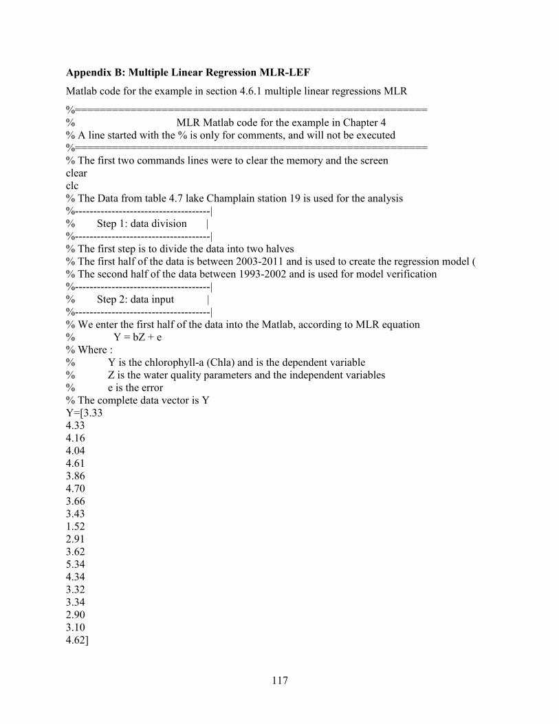
117

Appendix B: Multiple Linear Regression MLR-LEF

Matlab code for the example in section 4.6.1 multiple linear regressions MLR

%=========================================================

% MLR Matlab code for the example in Chapter 4

% A line started with the % is only for comments, and will not be executed

%=========================================================

% The first two commands lines were to clear the memory and the screen

clear

clc

% The Data from table 4.7 lake Champlain station 19 is used for the analysis

%-------------------------------------|

% Step 1: data division |

%-------------------------------------|

% The first step is to divide the data into two halves

% The first half of the data is between 2003-2011 and is used to create the regression model (

% The second half of the data between 1993-2002 and is used for model verification

%-------------------------------------|

% Step 2: data input |

%-------------------------------------|

% We enter the first half of the data into the Matlab, according to MLR equation

% Y = bZ + e

% Where :

% Y is the chlorophyll-a (Chla) and is the dependent variable

% Z is the water quality parameters and the independent variables

% e is the error

% The complete data vector is Y

Y=[3.33

4.33

4.16

4.04

4.61

3.86

4.70

3.66

3.43

1.52

2.91

3.62

5.34

4.34

3.32

3.34

2.90

3.10

4.62]

118

% The training data vector for the dependent variable

Y_train= [3.33

4.33

4.16

4.04

4.61

3.86

4.70

3.66

3.43

1.52]

% The verification data vector for the dependent variable

Y_verify= [2.91

3.62

5.34

4.34

3.32

3.34

2.90

3.10

4.62]

The complete independent Z matrix

z = [1993 100 13.89 11495.00 433.75 14.02 5.13 51.57 ;

1994 100 12.22 11594.44 466.33 12.68 5.33 49.50 ;

1995 100 8.97 12661.11 452.22 9.80 6.41 52.41 ;

1996 100 10.84 12461.70 447.08 8.90 4.88 50.38 ;

1997 100 11.37 11733.89 453.33 12.00 4.87 50.45 ;

1998 100 11.36 11879.17 396.25 12.53 5.20 50.37 ;

1999 100 10.64 12310.26 444.05 21.67 6.57 49.03 ;

2000 100 11.71 12622.00 427.17 16.78 6.04 49.14 ;

2001 100 10.51 13099.00 430.50 19.98 5.46 49.26 ;

2002 100 7.90 13633.33 403.67 22.24 6.50 48.20 ;

2003 100 8.57 14706.25 409.33 21.06 6.87 48.23 ;

2004 100 12.50 14775.28 398.50 16.53 6.11 49.31 ;

2005 100 12.57 15118.33 409.47 19.34 4.84 51.48 ;

2006 100 14.48 14686.31 435.12 19.60 4.42 49.83 ;

2007 100 12.87 13760.00 432.58 19.18 4.94 49.84 ;

2008 100 13.89 14448.33 436.00 18.20 5.40 49.42 ;

2009 100 12.75 14293.06 410.14 18.03 5.62 51.32 ;

2010 100 12.96 13975.71 370.29 13.00 4.60 53.72 ;

2011 100 16.12 12978.10 387.19 6.10 3.48 51.35 ]

% Following is the section of Z matrix that will be used for training and model creation

z_train = [1993 100 13.89 11495.00 433.75 14.02 5.13 51.57;

1994 100 12.22 11594.44 466.33 12.68 5.33 49.50 ;

1995 100 8.97 12661.11 452.22 9.80 6.41 52.41 ;

1996 100 10.84 12461.70 447.08 8.90 4.88 50.38 ;

119

1997 100 11.37 11733.89 453.33 12.00 4.87 50.45 ;

1998 100 11.36 11879.17 396.25 12.53 5.20 50.37 ;

1999 100 10.64 12310.26 444.05 21.67 6.57 49.03 ;

2000 100 11.71 12622.00 427.17 16.78 6.04 49.14 ;

2001 100 10.51 13099.00 430.50 19.98 5.46 49.26 ;

2002 100 7.90 13633.33 403.67 22.24 6.50 48.20 ]

% The section of Z matrix which will be used for model verification

z_verify = [2003 100 8.57 14706.25 409.33 21.06 6.87 48.23 ;

2004 100 12.50 14775.28 398.50 16.53 6.11 49.31 ;

2005 100 12.57 15118.33 409.47 19.34 4.84 51.48 ;

2006 100 14.48 14686.31 435.12 19.60 4.42 49.83 ;

2007 100 12.87 13760.00 432.58 19.18 4.94 49.84 ;

2008 100 13.89 14448.33 436.00 18.20 5.40 49.42 ;

2009 100 12.75 14293.06 410.14 18.03 5.62 51.32 ;

2010 100 12.96 13975.71 370.29 13.00 4.60 53.72 ;

2011 100 16.12 12978.10 387.19 6.10 3.48 51.35 ]

%-------------------------------------|

% Step 3: calculation of Beta |

%-------------------------------------|

% The best linear model is found when the error=0, thus the linear regression model becomes

% Y = bZ + e

% Using the training values we can find the coefficient matrix B, where Beta = b=Y/Z

% Since we will use the training data set we will rewrite the above equation

% b_hat = Y_train/z_train

% We can’t directly obtain the value of b_hat since z_train and Y_train

% are of different dimensions.

% To get around this problem we know that a matrix can be decomposed into

% two orthogonal matrices, therefore we can decompose the Z matrix into Q and R

% z_train matrix into Q and R

% Q is orthogonal matrix with n by p dimensions

% R is triangular p by p matrix

% Thus b_hat = z_train/Y_train = R\(Q'* Y_train)

% The last equation is the same as the least square equation

% Using the info on the Z matrix, we can define n and p

n=10; % the number of observations.

p=8; % the number of independent variables.

% The Matalb command to decompose z matrix into two orthogonal matrices is

[Q,R] = qr(z_train,0);

% Now to can calculate b_hat = Y_train/z_train = R\(Q'* Y_train)

b_hat = R\(Q'* Y_train);

%-------------------------------------|

% Step 3: Prediction |

%-------------------------------------|

% Beta matrix can be used in the linear regression equation

% Y = bZ + e

% To predict the values for the verification data set so

120

% % Yhat = z_verify * b_hat = z_train*(R\(Q'*Y_trtain));

Y_hat= z_verify*b_hat;

% where Yhat is n by 1 vector of fitted (or predicted) values of Y.

%-------------------------------------|

% Step 4: Verification |

%-------------------------------------|

% The predicted Yhat is compared to Y_verify using the error and

% the R Pearson correlation coefficient and R^2 the coefficient of determination

e = Y_verify -Y_hat;

% The mean squared error is defined as

mse = e'*e./(n-p);

%Square the residuals and total them to obtain the residual sum of squares:%

SSresid = sum (e. ^2);

% Compute R Pearson correlation coefficient

r=corr(Y_verify , Y_hat);

% Compute R^2 coefficient of determination

rsq =r^2;

%-------------------------------------|

% Step 5 : Output |

%-------------------------------------|

% The results are plotted analysis

Plot(Y_verify ,'r-', 'LineWidth', 2);

% Label the curve for function f in red

Text(7.5, 5.4, 'Y Observed Chla', 'Color', 'r', 'LineWidth', 2);

Hold all

Plot(Y_hat,'b-', 'LineWidth', 2);

Text(7.5, 5.2, 'Yhat Predcited Chla', 'Color', 'b', 'LineWidth', 2);

xlabel('x=Years 2003 to 2011','FontSize',12);

ylabel('Chla concentration μg/L’,'FontSize',12);

121

Appendix C: Multiple Nonlinear Regressions

The concept in developing a nonlinear regression model is based on understanding the

distribution shape of the data under investigation. First we search for a known nonlinear function

that shares a similar shape for the data distribution in question, then by MNR model is obtained

by adjusting the coefficients of the known nonlinear function to fit in the data distribution.

Figure C.1 is a screen shot for the IBM SPSS multiple nonlinear regression setup menu,

illustrating where a known nonlinear a function is required to commence with MNR modeling.

Figure C.1 IBM SPSS, MNR setup menu

The first task is to start with the MNR modeling to find a nonlinear function that shares

similar shape to chlorophyll-a observed data distribution for Lake Champlain, for this step the

chlorophyll-a observed data distribution records for the 15 monitoring stations of lake Champlain

are presented in table C.1 is plotted as a graph on figure C.2

From figure C.2 we notice that almost each station has its unique oscillating shape and

that there isn’t a common or specific function that can be used to describe the distribution of all

the stations; consequently, we can’t proceed with the multiple nonlinear analysis

122

Table C.1 Chla yearly data records for lake Champlain

Figure C.2 Lake Champlain Chla yearly data

Year

Chla

02

Chla

04

Chla

07

Chla

09

Chla

16

Chla

19

Chla

21

Chla

25

Chla

34

Chla

33

Chla

34

Chla

36

Chla

40

Chla

46

Chla

50

Chla

51

1992 8.11 9.15 5.63 4.74 5.48 3.88 5.84 6.08 5.84 5.57 4.8 9.5

1993 7.04 4.62 5.25 3.33 4.07 3.08 5.37 4.76 5.37 4.5 7.2

1994 6.52 8.37 5.27 4.33 5.25 3.3 4.11 4.26 4.11 5.36 4.17 7.85

1995 10.79 6.85 3.05 4.16 3.86 2.8 4.86 3.87 4.86 3.54 6.57 4.12

1996 5.77 5.67 4.44 4.04 3.91 3.49 4.38 3.86 4.38 3.71 8.69 4.54 25.77

1997 5.16 5.01 4.78 4.61 3.99 4.02 5.95 4.14 5.95 4.28 12.01 3.26 10.58

1998 4.25 7.28 4.72 3.86 4.72 4.66 5.01 3.38 5.01 4.74 8.38 3.09 9.63

1999 6.51 6.63 6.83 4.7 5.43 4.38 5.22 4 5.22 3.05 15 2.74 29.56

2000 5.85 5.22 5.98 3.66 4.56 2.87 9.12 3.77 9.12 2.73 17.66 2.37 6.72

2001 6.45 6.61 3.49 3.02 3.25 3.43 2.95 2.43 5.31 2.33 5.31 2.39 8.01

2002 5.09 4.57 1.82 2.19 1.83 1.52 2.11 2.46 4.28 1.76 4.28 2.2 13.86 1.32 9.16

2003 6.48 8.11 5.46 4.27 2.74 2.91 2.95 2.62 4.92 2.39 4.92 4.12 9.44 2.28 12.64

2004 5.36 10.53 5.45 3.69 4 3.62 3.84 3.33 6.77 3.08 6.77 4.17 7.77 4.61

2005 11.92 11.82 10.34 6.52 4.98 5.34 4.59 2.66 6.21 3.43 6.21 3.76 8.62 4.76 11.89

2006 5.04 6.25 6.17 6.26 4.47 4.34 4.2 3.15 6.37 4.27 6.37 8.89 2.69 12.36 19.53

2007 9.09 7.02 4.92 3.82 3.02 3.32 3.18 3.45 4.54 2.56 4.54 3.4 3.39 9.27 10.91

2008 6.63 6.1 4.8 4.82 3.6 3.34 3.27 3.13 4.89 3.8 4.89 8.66 2.77 15.79 13.52

2009 7.7 6.2 4.9 5.3 3.69 2.9 4.05 3.2 4.98 2.38 4.98 3.38 5.54 1.95 7.92 11.41

2010 7.26 6.59 4.87 3.64 3.44 3.1 3.2 2.88 2.64 3.57 4.23 16.83 15.34

2011 10.66 16.65 6.25 5.22 5.53 4.62 4.04 2.83 5.25 4.7 5.25 7.97 3.66 10.99 16.06

123

Appendix D:

D.1 Data Mining Results for Entire Lake Data

Chla = 4.83662 + 2.63347e-7*TP*Secchi*TN^2 + 2.63347e-

7*TP*TN^2*cos(0.0663525 + Year) - 0.75498*Secchi

Chla = 4.8539 + 2.63347e-7*TP*Secchi*TN^2 + 2.63347e-

7*TP*TN^2*cos(Year) - 0.75498*Secchi

Chla = 4.78993 + 2.63347e-7*TP*Secchi*TN^2 +

2.55028*cos(Year)/(0.0752586 + Secchi) - 0.753823*Secchi

Chla = 4.7918 + 2.4918*cos(Year)/Secchi + 2.63347e-

7*TP*Secchi*TN^2 - 0.753823*Secchi

124

D.2 Data Mining Results for Main Lake Data (Without Stations 02,04,50 and 51)

Chla = 1.660 + (TP*RegAlk + 228.652*cos(-0.870*Year) +

219.920*cos(2085.364*cos(-0.8577*Year)))/(44.149*Secchi +

TempC*Secchi)

Chla = 1.758 + (0.015*TP*RegAlk + 3.602*cos(-0.870*Year) +

3.725*cos(2085.391*cos(-0.857*Year)))/Secchi

Chla = 1.849 + (0.014*TP*RegAlk + 3.973*cos(2085.427*cos(-

0.857*Year)))/Secchi + cos(-0.889*Year)

Chla = 1.730 + (TP*RegAlk + 236.708*cos(-0.851*Year) +

175.643*cos(1.363*Year))/(46.559*Secchi + TempC*Secchi)

D.3 Data Mining Results for North Lake Data Stations 50 and 51

125

Chla = 38.493*10-5

*TP*TN + 3.122*sin(Year - Cl -

cos(RegAlk))

Chla = 37.157*10-5

*TP*TN + 2.178*sin(5.974 + Year - Cl)

Chla = 5.940*Depth + 0.0422*TP*sin(7.1271*Year) - 13.99

Chla = 5.908*Depth + 1.834*sin(7.123*Year) - 13.829

D.4 Data Mining Results for South Lake Data Stations 02 and 04

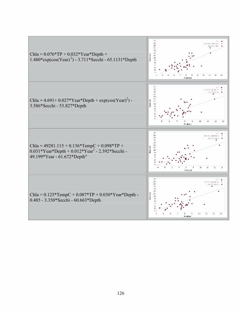
126

Chla = 0.076*TP + 0.032*Year*Depth +

1.480*exp(cos(Year) 2

) - 3.711*Secchi - 65.1131*Depth

Chla = 4.691+ 0.027*Year*Depth + exp(cos(Year)2) -

3.586*Secchi - 53.827*Depth

Chla = 49281.115 + 0.136*TempC + 0.098*TP +

0.031*Year*Depth + 0.012*Year2 - 2.392*Secchi -

49.199*Year - 61.672*Depth"

Chla = 0.125*TempC + 0.087*TP + 0.030*Year*Depth -

0.485 - 3.350*Secchi - 60.663*Depth

CONCORDIA UNIVERSITY A GIS BASED MODELLING APPROACH …

Documents

Transcript of CONCORDIA UNIVERSITY A GIS BASED MODELLING APPROACH …