Computer Vision

ECE/CSE 576Color and Texture

Linda ShapiroProfessor of Computer Science & Engineering

Professor of Electrical & Computer Engineering

We don’t really understand vision

- Visual cortex - highly studied part of the brain- Only rough idea of what different components do- New discoveries in vision all the time

- Eye uses blinking to reset its rotational orientation- Visual cortex can make some “high-level” decisions

Is vision easy or hard for humans?- What do you think?

Is vision easy or hard for humans?- What do you think now?

Objects reflect only some light

We can make a map of color

Linear colorspace- Pick some primaries- Can mix those primaries to match any color inside the triangle- There is a commision that studies color!

- Commission internationale de l’éclairage (CIE) is a 100 year old organization that creates international standards related to light and color.

“Theoretical” CIE RGB primaries

Practical sRGB primaries, MSFT 1996

sRGB (standard Red Green Blue) is an RGB color space that HP and Microsoft created cooperatively in 1996 to use on monitors, printers, and the Internet. It was subsequently standardized by the IEC (International Electrotechnical Commission) as IEC 61966-2-1:1999.

What does this mean for computers?- We represent images as grids of pixels

- Each pixel has a color, 3 components: RGB

- Not every color can be represented in RGB!- Have to go out in the real world sometimes

- RGB is not fully accurate

- We can represent a color with 3 numbers

- #ff00ff; (1.0, 0.0, 1.0); 255,0,255

- WHAT COLOR IS THAT?

11

FF00AA

Image: 2d array of color- Some range

- [0,255]

- 0.0 - 1.0

- We’ll talk more about

this later.

Grayscale - making color images not- We can simulate monochromatic images from RGB- Want a good approximation of how “bright” the image is without

color information- (R+B+G/3) - looks weird- We should

- Gamma decompress- Calculatight lightness- Gamma compress

- We can just operate on sRGB

- Typically ~ .30R + .59G + .11B

RGB is a cube...

Hue, Saturation, Value: cylinder!

Hue, Saturation, Value- Different model based on perception of light- Hue: what color- Saturation: how much color- Value: how bright- Allows easy image transforms

- Shift the hue- Increase saturation

Other colorspaces are fun!

Geometric HSV to RGB:

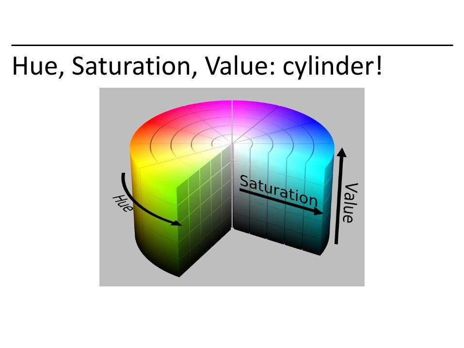
An RGB Image

19

Still 3d tensor, different info

Hue Saturation Value

More saturation = intense colors

2x

H Channel S Channel V Channel

More value = lighter image

2x

H Channel S Channel V Channel

Shift hue = shift colors

-.2

H Channel S Channel V Channel

Set hue to your favorite color!H Channel S Channel V Channel

Or pattern...H Channel S Channel V Channel

Increase and threshold saturationH Channel S Channel V Channel

More Details on Color Spaces• RGB• HSI/HSV• CIE L*a*b• YIQ• Opponent

standard for camerasallows us to separateintensity plus 2 color channelscolor TVs, Y is intensityused in Swain & Ballard work

RGB Color Space

30

red

blue

green

(0,0,0)

(0,0,255)

(0,255,0)

(255,0,0)

R,G,B)

Normalized red r = R/(R+G+B)

Normalized green g = G/(R+G+B)

Normalized blue b = B/(R+G+B)

Absolute Normalized

Color hexagon for HSI (HSV)• Hue is encoded as an angle (0 to 2).

• Saturation is the distance to the vertical axis (0 to 1).

• Intensity is the height along the vertical axis (0 to 1).

intensity

saturation

hue

H=0 is redH=180 is cyan

H=120 is green

H=240 is blue

I=0

I=1

31

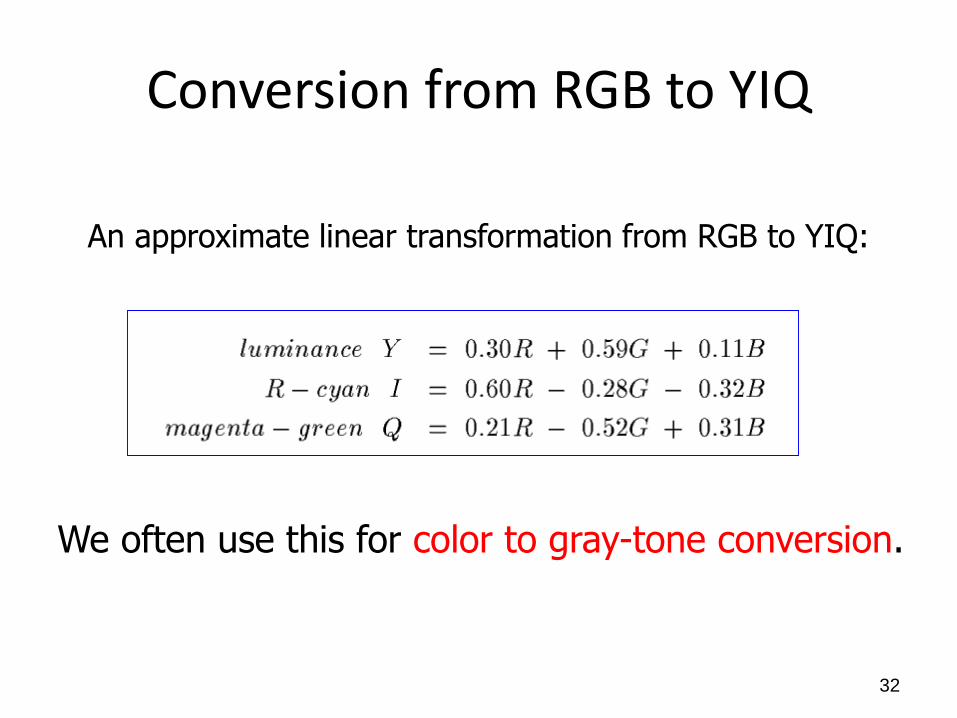
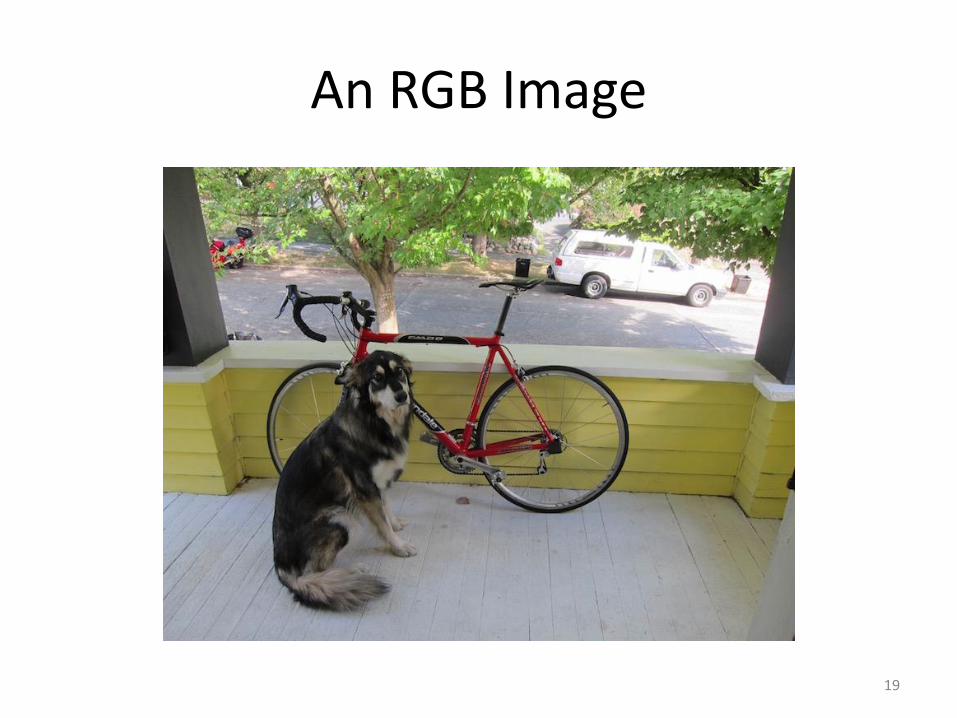
Conversion from RGB to YIQ

We often use this for color to gray-tone conversion.

An approximate linear transformation from RGB to YIQ:

32

CIELAB, Lab, L*a*b• One luminance channel (L)

and two color channels (a and b).

• In this model, the color differences which you perceive correspond to Euclidian distances in CIELab.

• The a axis extends from green (-a) to red (+a) and the b axis from blue (-b) to yellow (+b). The brightness (L) increases from the bottom to the top of the three-dimensional model.

33

CIE L*a*b* (CIELAB) is a color space specified by the International Commission on Illumination (French Commission internationale de l'éclairage, hence its CIE initialism).

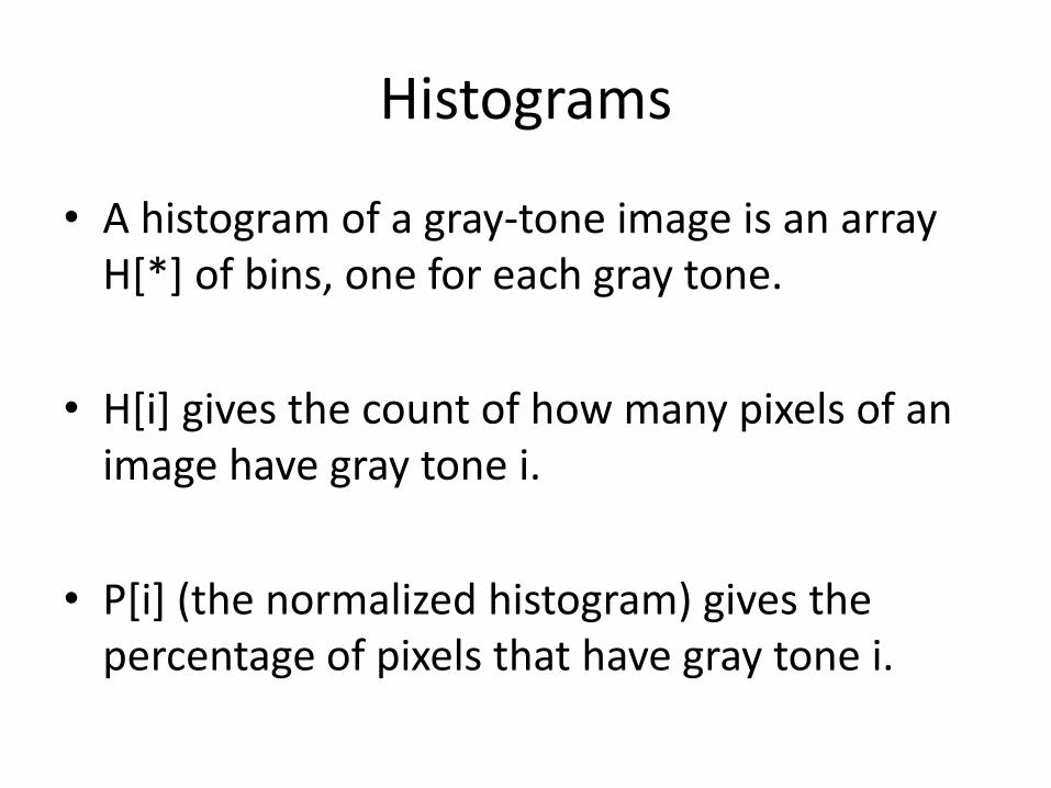
Histograms

• A histogram of a gray-tone image is an array H[*] of bins, one for each gray tone.

• H[i] gives the count of how many pixels of an image have gray tone i.

• P[i] (the normalized histogram) gives the percentage of pixels that have gray tone i.

Color histograms can represent an image

• Histogram is fast and easy to compute.

• Size can easily be normalized so that different image histograms can be compared.

• Can match color histograms for database query or classification.

35

Histograms of two color images

36

Apples versus Oranges

Separate HSI histograms for apples (left) and oranges (right) used by IBM’s VeggieVision for recognizing produce at the grocery store checkout station (see Ch 16).

H

S

I

37

Skin color in Normalized R-G Space

Purple region shows skin color samples from several people. Blue and yellow regions show skin in shadow or behind a beard.

38R normalized

G normalized

Finding a face in video frame

• (left) input video frame

• (center) pixels classified according to RGB space

• (right) largest connected component with aspect similar to a face (all work contributed by Vera Bakic)

39

Swain and Ballard’s Histogram Matchingfor Color Object Recognition

(IJCV Vol 7, No. 1, 1991)

Opponent Encoding:

Histograms: 8 x 16 x 16 = 2048 bins

Intersection of image histogram and model histogram:

Match score is the normalized intersection:

• wb = R + G + B• rg = R - G• by = 2B - R - G

intersection(h(I),h(M)) = min{h(I)[j],h(M)[j]}

match(h(I),h(M)) = intersection(h(I),h(M)) / h(M)[j]

j=1

numbins

j=1

numbins

40

(from Swain and Ballard)

cereal box image 3D color histogram

41

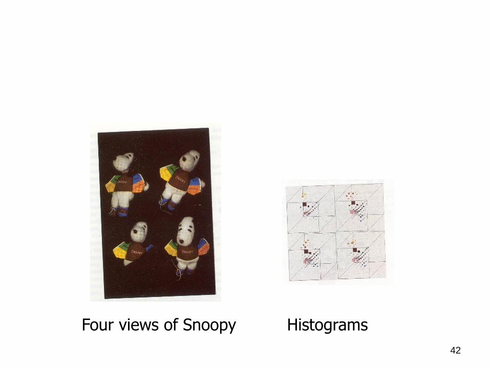
Four views of Snoopy Histograms

42

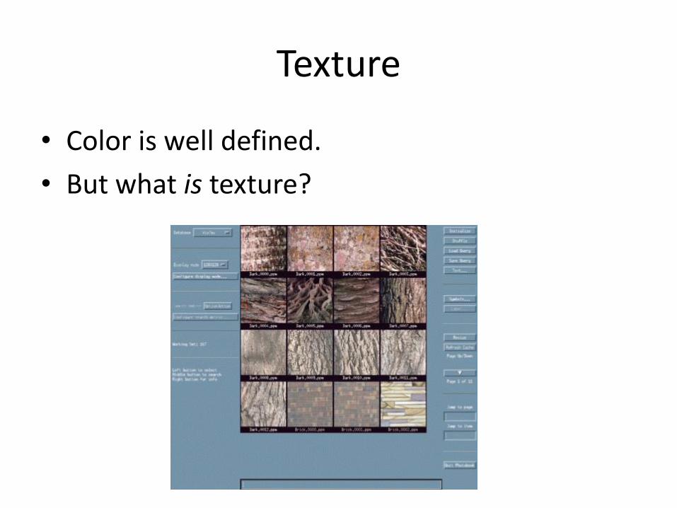
Texture

• Color is well defined.

• But what is texture?

Structural Texture

Texture is a description of the spatial arrangement of color or

intensities in an image or a selected region of an image.

Structural approach: a set of texels in some regular or repeated pattern

44

Natural Textures from VisTex

grass leaves

What/Where are the texels?45

The Case for Statistical Texture

• Segmenting out texels is difficult or impossible in real images.

• Numeric quantities or statistics that describe a texture can be

computed from the gray tones (or colors) alone.

• This approach is less intuitive, but is computationally efficient.

• It can be used for both classification and segmentation.

46

Local Binary Pattern Measure

100 101 103

40 50 80

50 60 90

• For each pixel p, create an 8-bit number b1 b2 b3 b4 b5 b6 b7 b8,

where bi = 0 if neighbor i has value less than or equal to p’s

value and 1 otherwise.

• Represent the texture in the image (or a region) by the

histogram of these numbers.

1 1 1 1 1 1 0 0

1 2 3

4

5

7 6

8

47

Fids (Flexible Image Database

System) is retrieving images

similar to the query image

using LBP texture as the

texture measure and comparing

their LBP histograms

Example

48

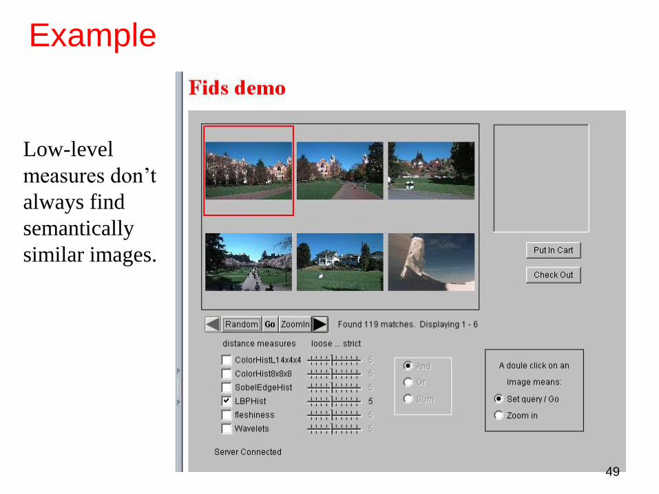
Low-level

measures don’t

always find

semantically

similar images.

Example

49

What else is LBP good for?

• We found it in a paper for classifying deciduous trees.

• We used it in a real system for finding cancer in Pap smears.

• We are using it to look for regions of interest in breast and melanoma biopsy slides.

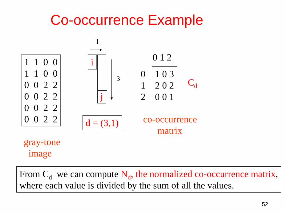
Co-occurrence Matrix Features

A co-occurrence matrix is a 2D array C in which

• Both the rows and columns represent a set of possible

image values.

• C (i,j) indicates how many times value i co-occurs with

value j in a particular spatial relationship d.

• The spatial relationship is specified by a vector d = (dr,dc).

d

51

1 1 0 0

1 1 0 0

0 0 2 2

0 0 2 2

0 0 2 2

0 0 2 2

j

i

1

3

d = (3,1)

0 1 2

0

1

2

1 0 3

2 0 2

0 0 1

Cd

gray-tone

image

co-occurrence

matrix

From Cd we can compute Nd, the normalized co-occurrence matrix,

where each value is divided by the sum of all the values.

Co-occurrence Example

52

Co-occurrence Features

sums.

What do these measure?

Energy measures uniformity of the normalized matrix.53

What are Co-occurrence Features used for?

• They were designed for recognizing different kinds of land uses in satellite images.

• They are still used heavily in geospatial domains, but they can be added on to any other calculated features.

Example

55

Satellite Image of Monterey Bay

Assignment 0

FUN WITH COLOR!

57

Image basics

• Data structure for an imagetypedef struct{

int h, w, c;

float *data;

} image;

58

Image basics

• Data structure for an imagetypedef struct{

int h, w, c;

float *data;

} image;

– h = height

–w = width

– c = number of channels

• c = 3 for RGB image; c = 1 for grayscale image

59

Image basics

• Data structure for an imagetypedef struct{

int h, w, c;

float *data;

} image;

– data = array of floats

– floats in the range [0,1]

– 3D image matrix linearized into 1D array

60

To Do #1

• Fill in:– float get_pixel(image im, int x, int y, int c)

– void set_pixel(image im, int x, int y, int c, float v)

• assign value v to im.data[coord(x,y,c)]

61

To Do #2

• Fill in:– image copy_image(image im)

• create a separate image that is a copy of the input image im and return the copy

• Useful functions:– make_image() in load_image.c

– memcpy()

• You can use get_pixel() and set_pixel()functions you implemented from now on

62

To Do #3

• Fill in:– image rgb_to_grayscale(image im)

• create a new image with 1 channel

• Get R,G,B values from input image im

• Compute Y = 0.299 R + 0.587 G + .114 B

• Assign Y to new image and return that image

63

To Do #4

• Fill in:– void shift_image(image im, int c, float v)

• add value v to each pixel of im in channel c

• change the input image in-place (do not create a separate image) wherever the return type of the function is void

64

To Do #5

• Fill in:– void clamp_image(image im)

• clamp the pixel values of input image im to be in the range [0,1]

65

To Do #6

• Fill in:– void rgb_to_hsv(image im)

• Convert R,G,B values of image im pixelwise into H,S,V values using the given formulas

• You can use the three_way_max() and three_way_min() functions provided

66

To Do #7

• Fill in:– void hsv_to_rgb(image im)

• Convert H,S,V values of image im pixelwise into R,G,B values using the given table

67

To Do #8 (extra credit)

• Fill in:– void scale_image(image im, int c, float v)

• multiply each pixel of im in channel c with value v

• add to the lines in image.h and other files as necessary to test the function. No need to submit the other edited files; write a comment in CAPS at the top of process_image.c if you attempt any extra credit

68

To Do #9 (super extra credit)

• Fill in:– void rgb_to_lch(image im)

• Convert R,G,B values of image im pixelwise into L,C,H values using the formulas in the given link

69

70

Have Fun