
ORT (other random topics) CSE P 576 Larry Zitnick ([email protected])[email protected].
84
-
Upload
helen-hampton -
Category
Documents
-
view
234 -
download
1
Transcript of ORT (other random topics) CSE P 576 Larry Zitnick ([email protected])[email protected].

Autonomous vehicles
• Navlab (1990’s)• Stanley (Offroad, 2004)• Boss (Urban, 2007)
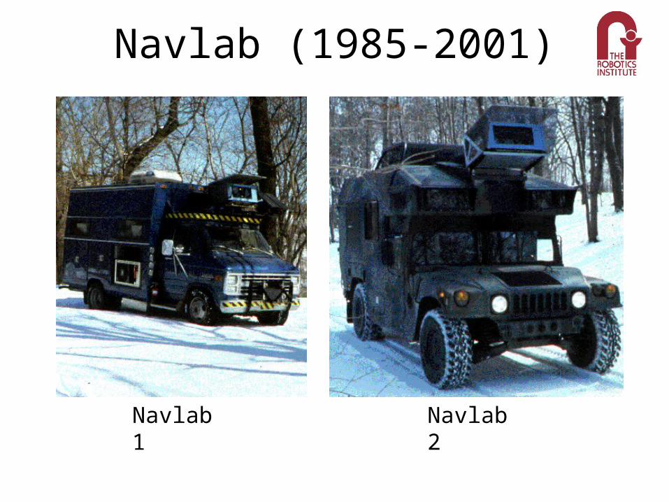
Navlab (1985-2001)
Navlab 1 Navlab 2

Navlab (1985-2001)
Navlab 5 Navlab 6

Navlab (1985-2001)
Navlab 10
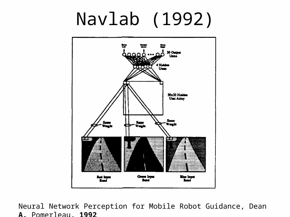
Navlab (1992)
Neural Network Perception for Mobile Robot Guidance, Dean A. Pomerleau, 1992

RALPH: Rapidly Adapting Lateral Position Handler, Dean Pomerleau, 1995
No Hands Across America
• 2797/2849 miles (98.2%) • The researchers handled the throttle and
brake. • When did it fail?
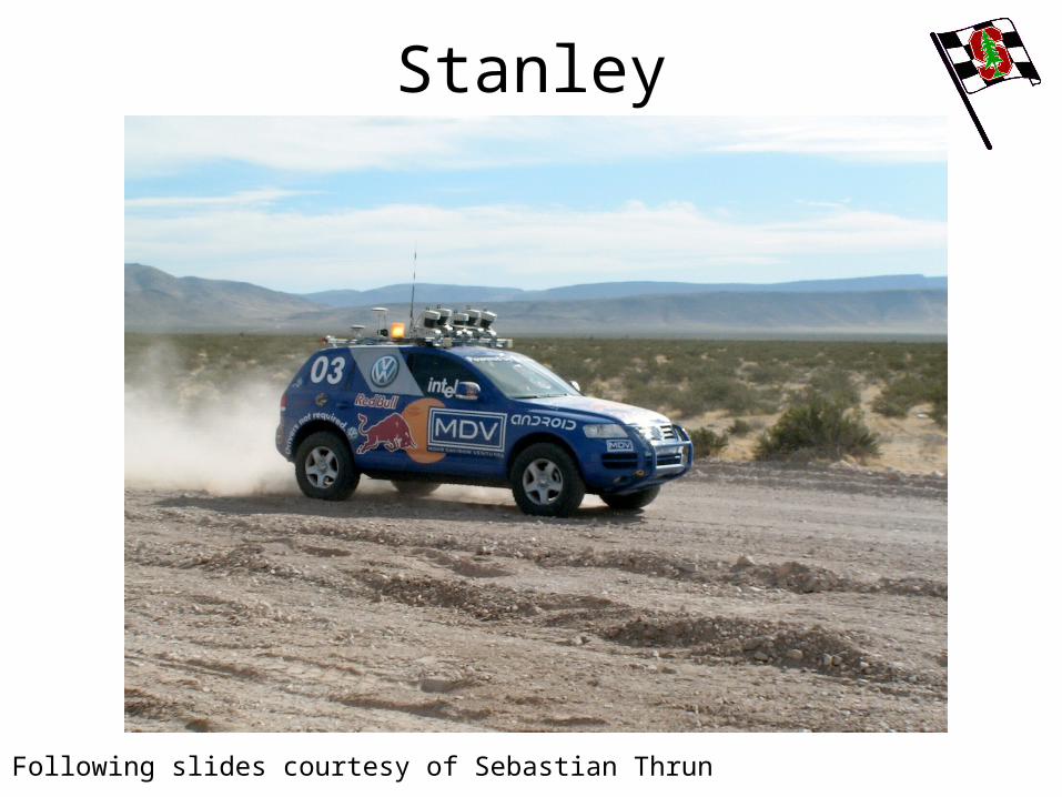
Stanley
Following slides courtesy of Sebastian Thrun
Stanford Racing Team
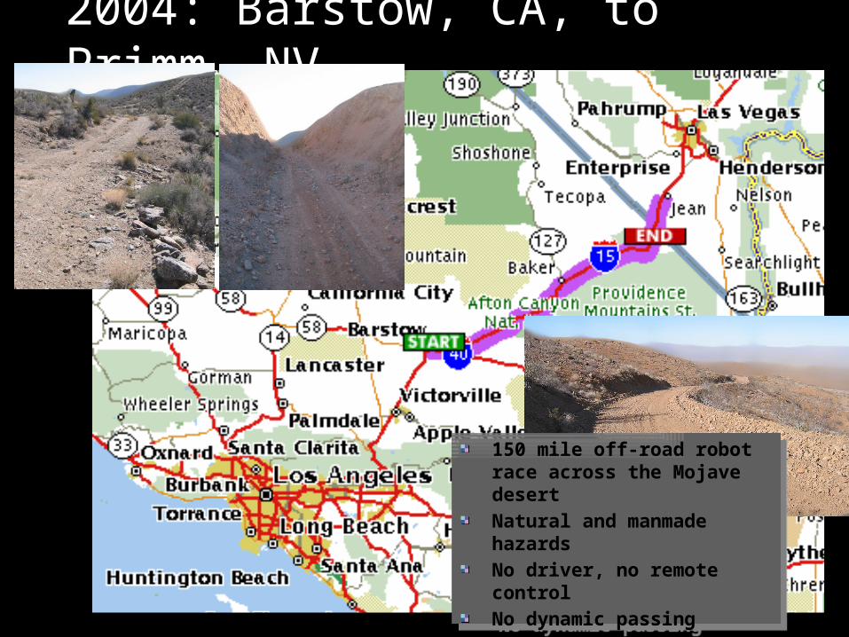
2004: Barstow, CA, to Primm, NV
150 mile off-road robot race across the Mojave desert
Natural and manmade hazards
No driver, no remote control
No dynamic passing
Fastest vehicle wins the race (and 2 million dollar prize)
150 mile off-road robot race across the Mojave desert
Natural and manmade hazards
No driver, no remote control
No dynamic passing
Fastest vehicle wins the race (and 2 million dollar prize)

Stanford Racing Team
Grand Challenge 2005: 195 Teams
Stanford Racing Team
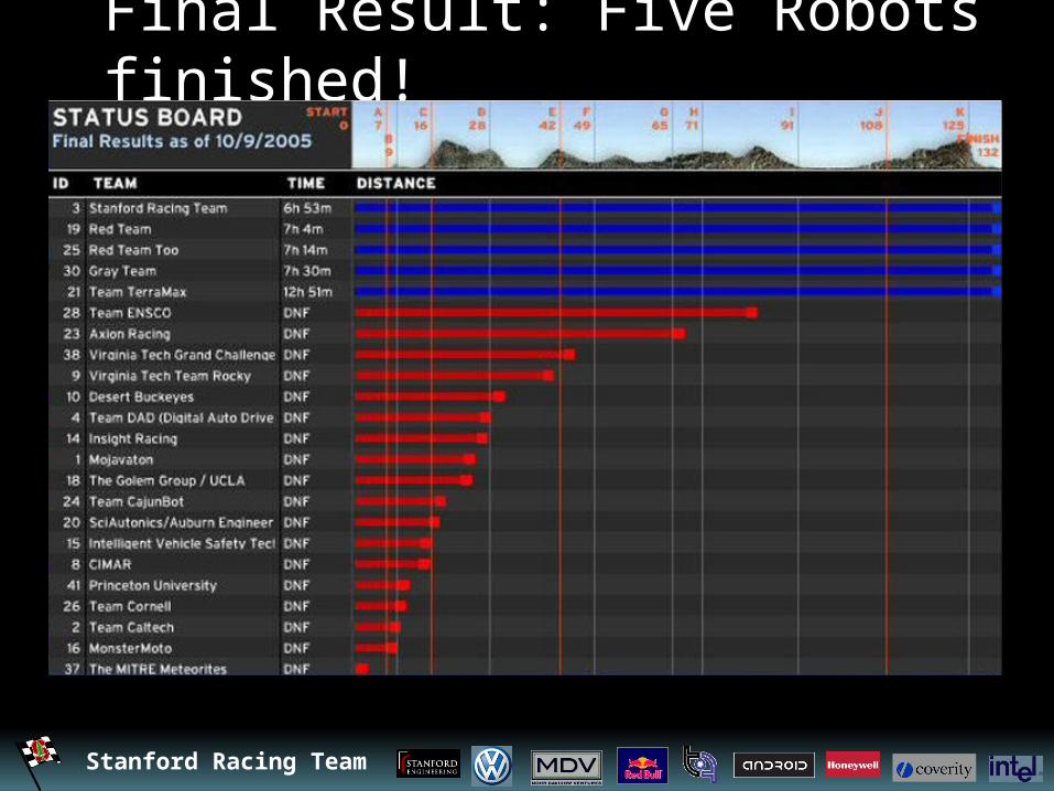
Final Result: Five Robots finished!

Stanford Racing Team
Manual Offroad Driving

Stanford Racing Team
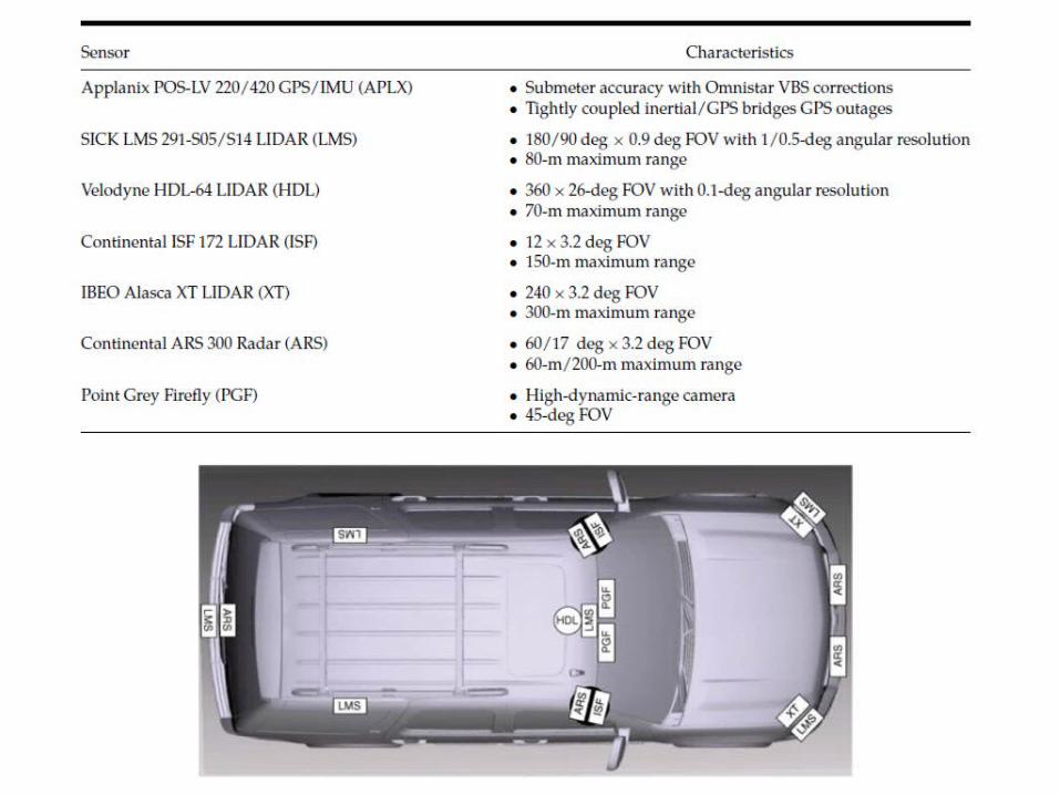
Software Architecture

Stanford Racing Team
Touareg interface
Laser mapper
Wireless E-Stop
Top level control
Laser 2 interface
Laser 3 interface
Laser 4 interface
Laser 1 interface
Laser 5 interface
Camera interface
Radar interface Radar mapper
Vision mapper
UKF Pose estimation
Wheel velocity
GPS position
GPS compass
IMU interface Surface assessment
Health monitor
Road finder
Touch screen UI
Throttle/brake control
Steering control
Path planner
laser map
vehicle state (pose, velocity)
velocity limit
map
vision map
vehiclestate
obstacle list
trajectory
RDDF database
driving mode
pause/disable command
Power server interface
clocks
emergency stop
power on/off
Linux processes start/stopheart beats
corridor
SENSOR INTERFACE PERCEPTION PLANNING&CONTROL USER INTERFACE
VEHICLEINTERFACE
RDDF corridor (smoothed and original)
Process controller
GLOBALSERVICES
health status
data
Data logger File system
Communication requests
vehicle state (pose, velocity)
Brake/steering
Communication channels
Inter-process communication (IPC) server Time server
road center
Stanley Software Architecture
Stanford Racing Team
Planning and Steering Control

Stanford Racing Team
Low-Level Steering Control
Planer Output
Cross-Track Error
Velocity
Steering Angle
(with respect to trajectory)
Stanford Racing Team
Discuss Kalman Filter
To the whiteboard…

Stanford Racing Team
Parameterizing Search SpaceLateral offsetRoad boundary

Stanford Racing Team
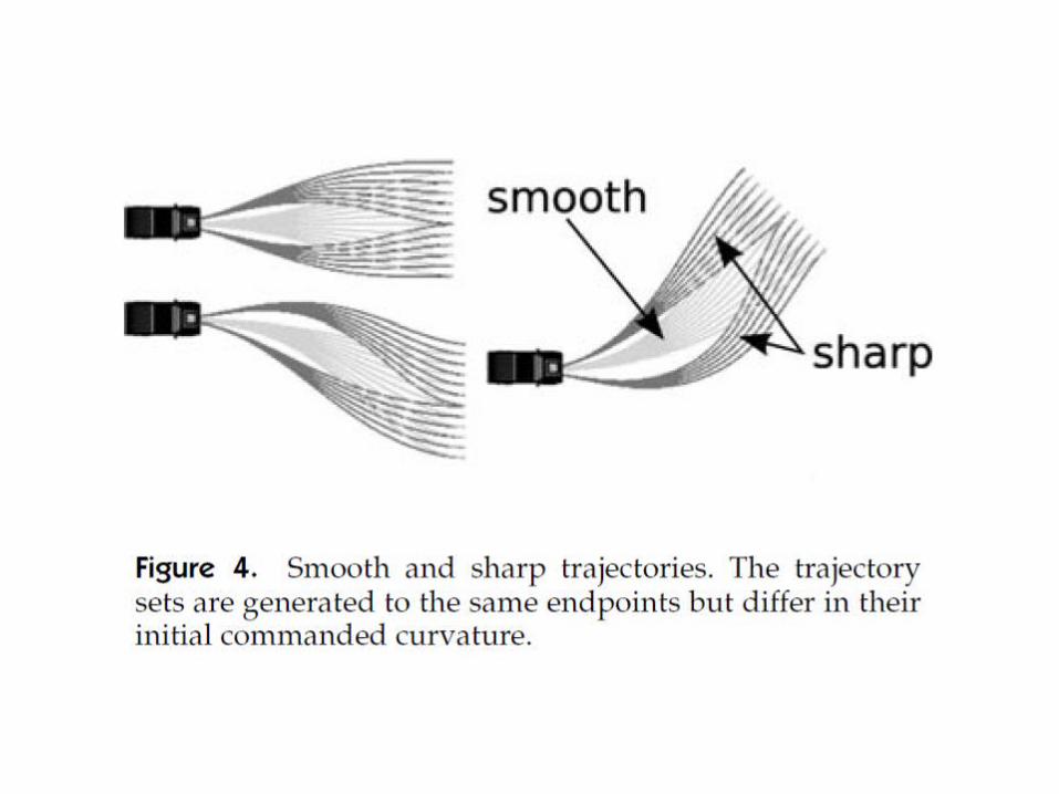
Planning = Rolling out Trajectories
Stanford Racing Team
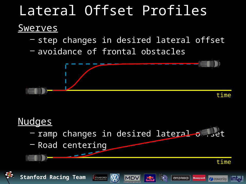
Lateral Offset ProfilesSwerves
– step changes in desired lateral offset– avoidance of frontal obstacles
Nudges– ramp changes in desired lateral offset– Road centering
time
time
Stanford Racing Team
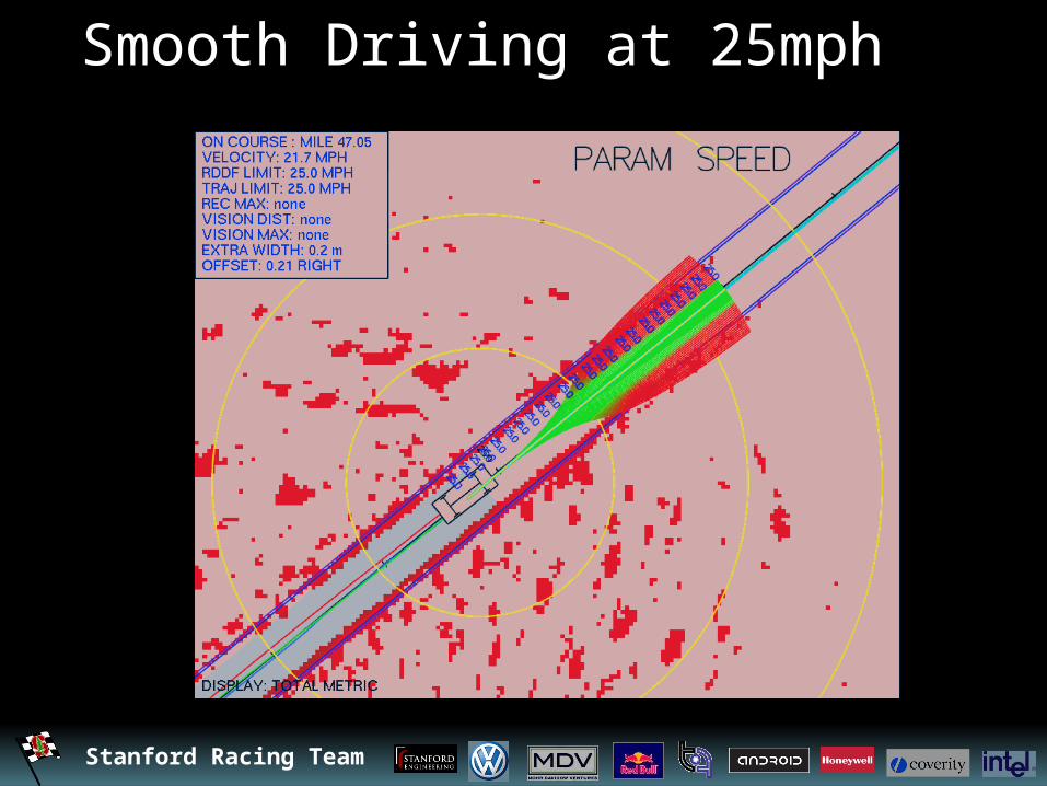
Smooth Driving at 25mph
Stanford Racing Team
Laser Terrain Mapping
Stanford Racing Team
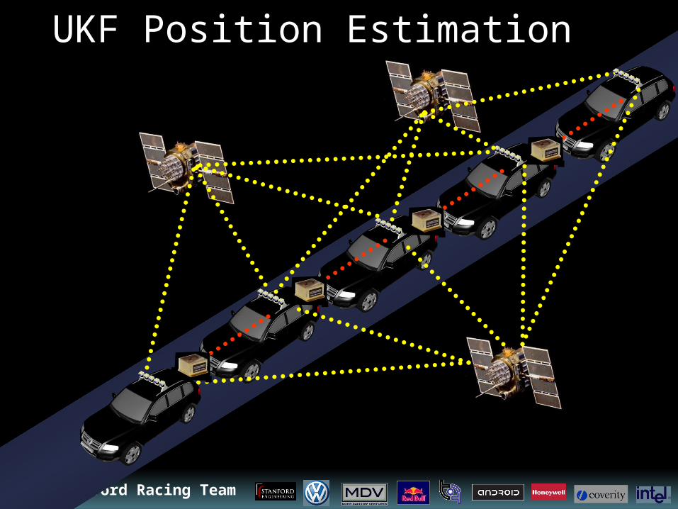
UKF Position Estimation
Stanford Racing Team
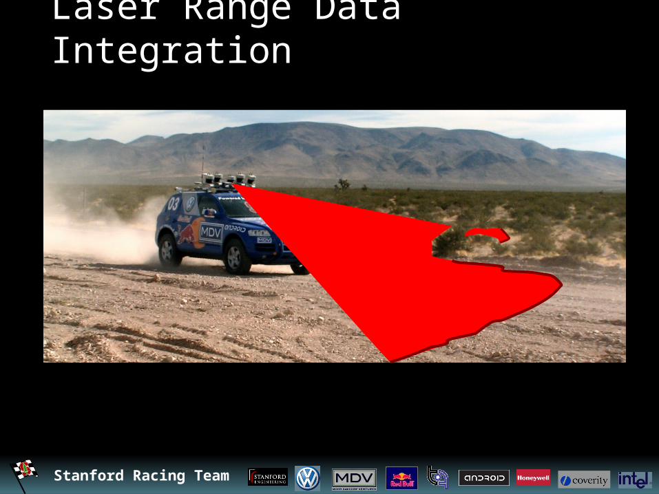
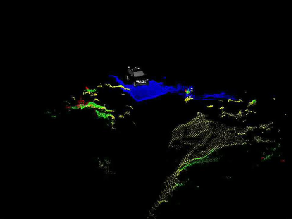
Laser Range Data Integration
Stanford Racing Team

Stanford Racing Team
Range Sensor Interpretation
12
3

Stanford Racing Team
Obstacle Detection
DZ
Stanford Racing Team
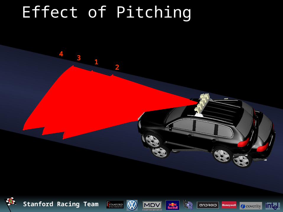
Effect of Pitching
12
34

Stanford Racing Team
Stanley….After Learning
With Learning: 0.02% false positivesWithout Learning: 12.6% false positives
Stanford Racing Team
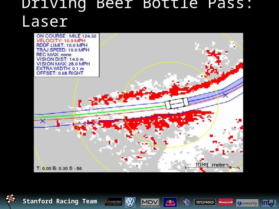
Driving Beer Bottle Pass: Laser
Stanford Racing Team
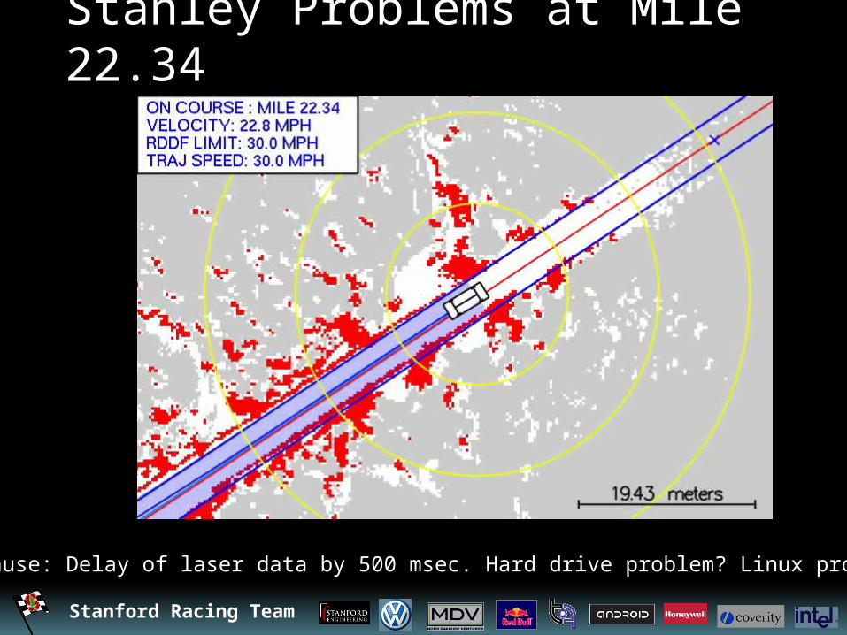
Stanley Problems at Mile 22.34
Cause: Delay of laser data by 500 msec. Hard drive problem? Linux problem?
Stanford Racing Team
Computer Vision Terrain Mapping

Stanford Racing Team
Limits of lasers
Lasers see 22m = 25mph
They needed to go 35mph to finish the race.

Stanford Racing Team
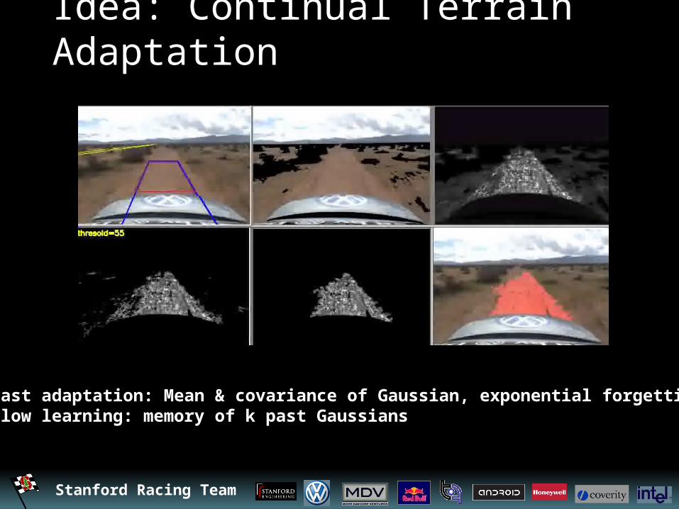
What Defines A Road?
Stanford Racing Team
Idea: Continual Terrain Adaptation
Fast adaptation: Mean & covariance of Gaussian, exponential forgettingSlow learning: memory of k past Gaussians

Stanford Racing Team
Adaptive Vision In Action (NQE)

Stanford Racing Team
Adaptive Vision in Mojave Desert

Stanford Racing Team
Driving Beer Bottle Pass: Vision
Stanford Racing Team
Speed Control

Stanford Racing Team
Speed Controllers
Throttle
Forward velocity
Brake pressureThrottle &
BrakeController
Throttle, Brake
DARPA Speed Limit
Vehicle pitch/roll
Vertical acceleration
Obstacles Clearance
CurvatureVelocity
Controller
target velocity
Vertical acceleration
target velocity
DARPA Speed Limit
Vehicle pitch/roll
Obstacles Clearance
Curvature

Stanford Racing Team
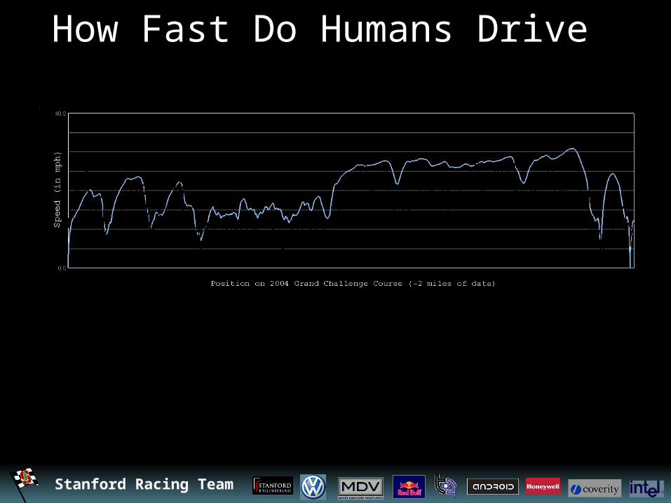
Controlling speed
If you hit a bump, slow down (that first pothole really hurts…)
If you haven’t hit a bump in awhile linearly increase speed.
Slow down on hills.
Stanford Racing Team
How Fast Do Humans Drive

Stanford Racing Team
Learning To Drive Like a Person
Sebastian
Stanley
Stanford Racing Team
More info
For full detail read the paper:
Stanley: The Robot that Won the DARPA Grand Challenge, Sebastian et al., Journal of Field Robotics, 2006

DARPA Urban Challenge
• 36 teams invited to National Qualification Event.
• 11 teams invited to Urban Challenge Final Event
Suddenly, the vehicle did a U-turn and headed directly at Tether’s vehicle. “Five of us in the vehicle were all yelling ‘pause!’” Tether recalled, referring to the pause command that DARPA could send to a vehicle.
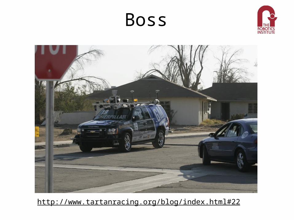
http://www.tartanracing.org/blog/index.html#22

Boss
CompactPCI chassis with 10 2.16-GHz Core2Duo processors, each with 2 GB of memory
2007 Chevrolet Tahoe

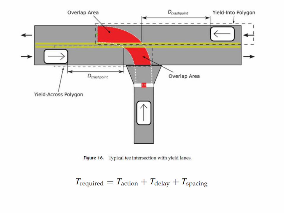
Motion planning
• Structured driving (road following)
• Unstructured driving (maneuvering in parking lots)

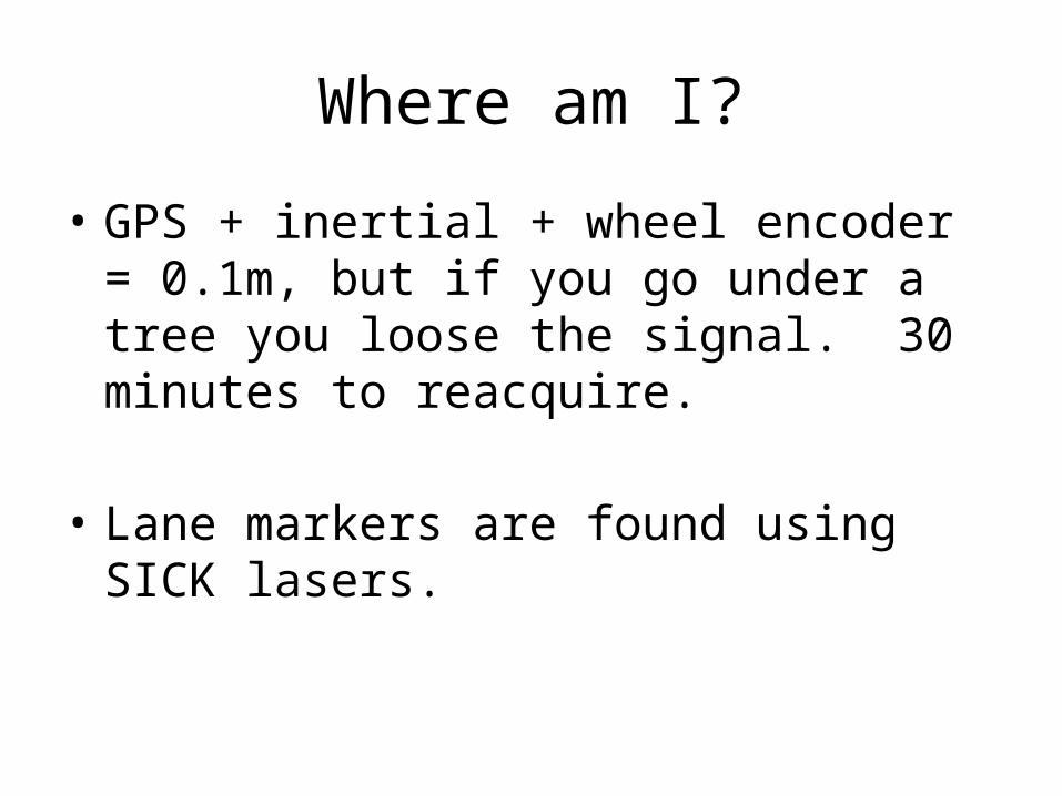
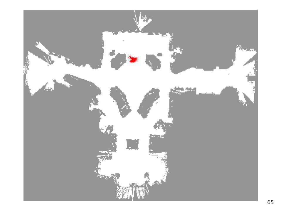
Where am I?
• GPS + inertial + wheel encoder = 0.1m, but if you go under a tree you loose the signal. 30 minutes to reacquire.
• Lane markers are found using SICK lasers.

Particle Filters
Particle filter slides courtesy of Sebastian Thrun

)|()(
)()|()()|()(
xzpxBel
xBelxzpw
xBelxzpxBel
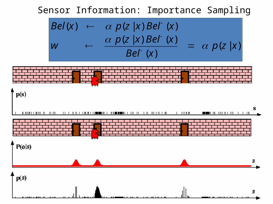
Sensor Information: Importance Sampling
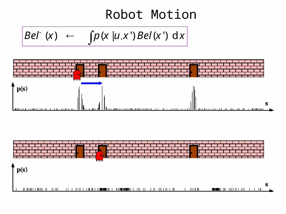
'd)'()'|()( , xxBelxuxpxBel
Robot Motion
)|()(
)()|()()|()(
xzpxBel
xBelxzpw
xBelxzpxBel
Sensor Information: Importance Sampling

Robot Motion
'd)'()'|()( , xxBelxuxpxBel
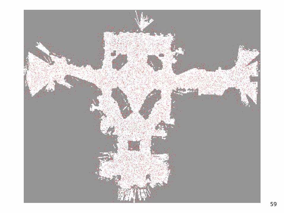
59

60
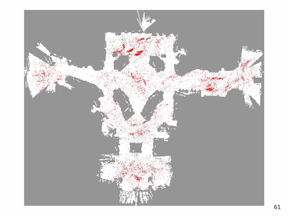
61

62
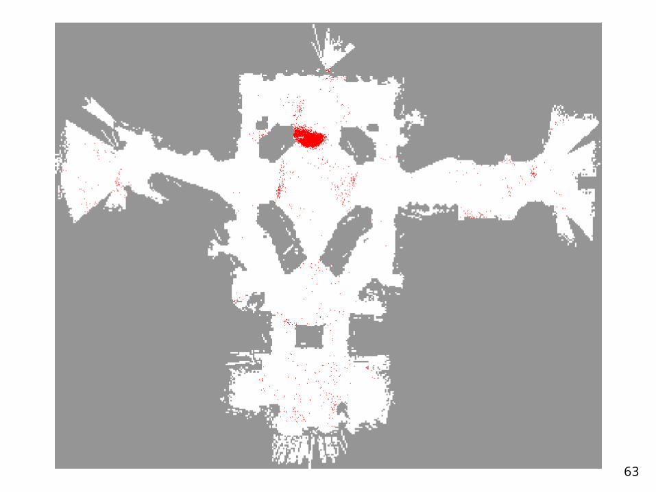
63

64
65
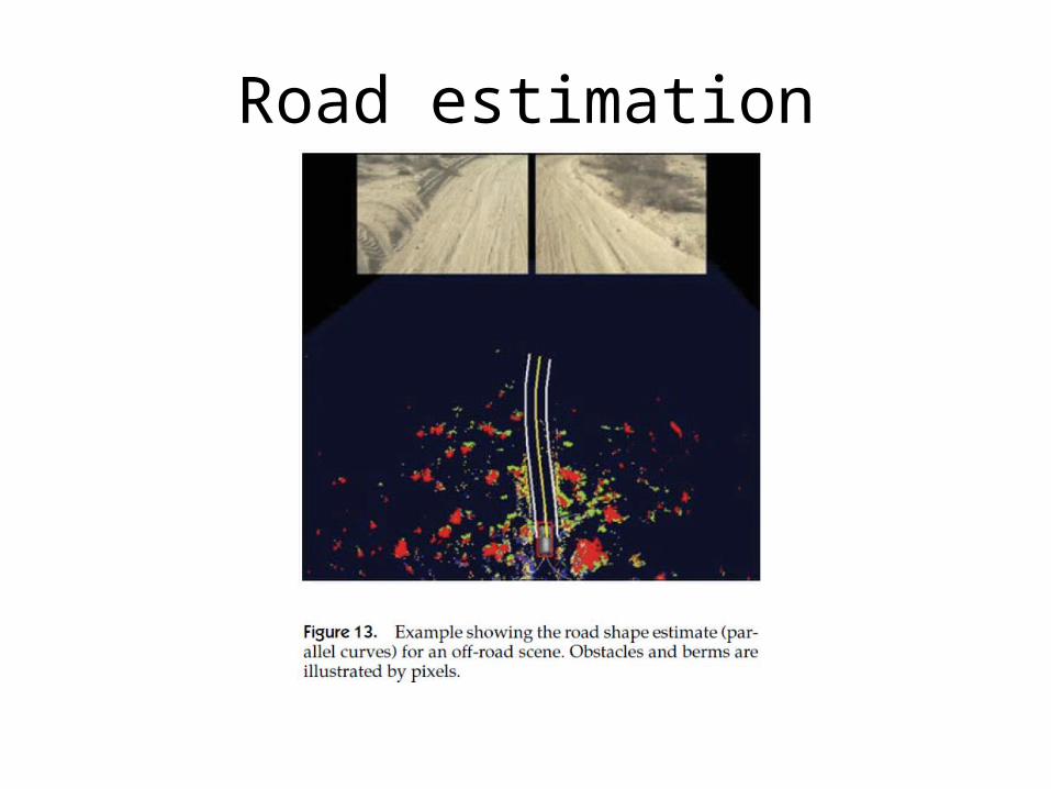
Road estimation

Failures

Failures

Failures
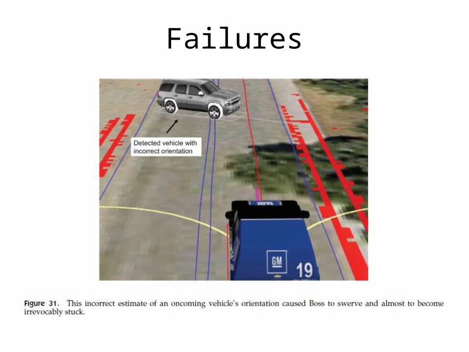
Failures

More info
Autonomous Driving in Urban Environments: Boss and the Urban Challenge, Urmson et al., Journal of Field Robotics, 2008
A Fast Approximation of the Bilateral Filter
using a Signal Processing Approach
Sylvain Paris and Frédo Durand
Computer Science and Artificial Intelligence Laboratory
Massachusetts Institute of Technology

space range
p
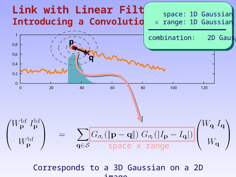
Link with Linear FilteringIntroducing a Convolution
q
space: 1D Gaussian range: 1D Gaussian
combination: 2D Gaussian
space: 1D Gaussian range: 1D Gaussian
combination: 2D Gaussian
p
Link with Linear FilteringIntroducing a Convolution
q
space: 1D Gaussian range: 1D Gaussian
combination: 2D Gaussian
space: 1D Gaussian range: 1D Gaussian
combination: 2D Gaussian
space x range
Corresponds to a 3D Gaussian on a 2D image.
Link with Linear FilteringIntroducing a Convolution
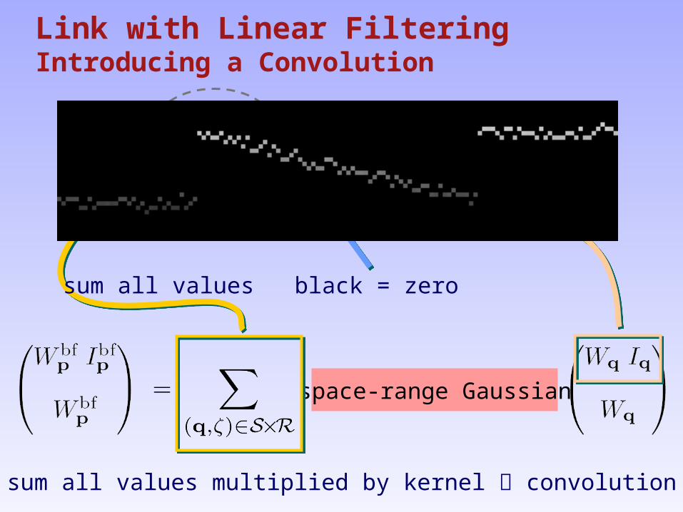
space-range Gaussian
black = zerosum all values
sum all values multiplied by kernel convolution
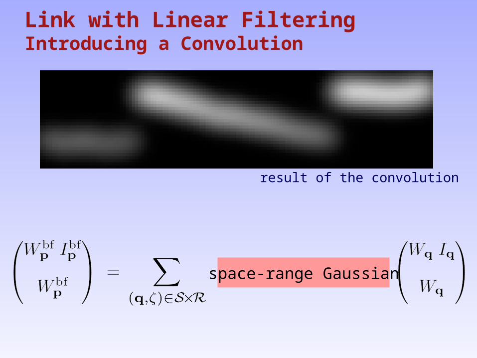
space-range Gaussian
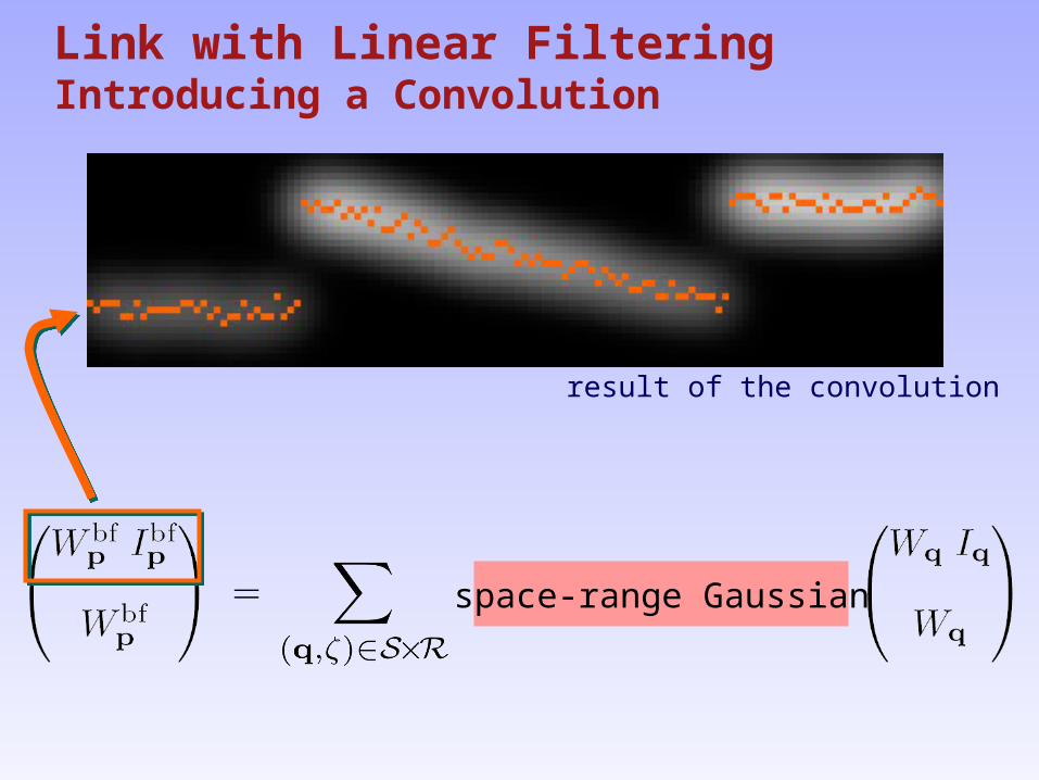
result of the convolution
Link with Linear FilteringIntroducing a Convolution
Link with Linear FilteringIntroducing a Convolution
space-range Gaussian
result of the convolution

higher dimensional functions
Gaussian convolution
division
slicing
w i w

higher dimensional functions
Gaussian convolution
division
slicing
Low-pass filter
Low-pass filter Almost only
low freq.
High freq. negligible
Almost onlylow freq.
High freq. negligible
w i w

higher dimensional functions
Gaussian convolution
division
slicing
w i w
D O W N S A M P L E
U P S A M P L E
Almost noinformation
loss
Almost noinformation
loss

Accuracy versus Running Time• Finer sampling increases accuracy.• More precise than previous work.
finer sampling
PSNR as function of Running TimeDigital
photograph1200 1600
Straightforward implementation is over 10 minutes.

Visual Results
input exact BF our result prev. work
1200 1600
• Comparison with previous work [Durand 02]– running time = 1s for both techniques
0
0.1differencewith exact
computation(intensities in [0:1])

More advanced approaches:
http://graphics.stanford.edu/papers/gkdtrees/
http://graphics.stanford.edu/papers/permutohedral/