Compressed Video Action Recognition

Chao-Yuan Wu1,5∗

cywu@cs.utexas.edu

Manzil Zaheer2,5∗

manzil@cmu.edu

Hexiang Hu3,5∗

hexiangh@usc.edu

R. Manmatha4

manmatha@a9.com

Alexander J. Smola5

smola@amazon.com

Philipp Krahenbuhl1

philkr@cs.utexas.edu

1The University of Texas at Austin, 2Carnegie Mellon University,3University of Southern California, 4A9, 5Amazon

AbstractTraining robust deep video representations has proven to

be much more challenging than learning deep image repre-sentations. This is in part due to the enormous size of rawvideo streams and the high temporal redundancy; the trueand interesting signal is often drowned in too much irrel-evant data. Motivated by that the superfluous informationcan be reduced by up to two orders of magnitude by videocompression (using H.264, HEVC, etc.), we propose to traina deep network directly on the compressed video.

This representation has a higher information density,and we found the training to be easier. In addition, the sig-nals in a compressed video provide free, albeit noisy, motioninformation. We propose novel techniques to use them effec-tively. Our approach is about 4.6 times faster than Res3Dand 2.7 times faster than ResNet-152. On the task of actionrecognition, our approach outperforms all the other meth-ods on the UCF-101, HMDB-51, and Charades dataset.

1. IntroductionVideo commands the lion’s share of internet traffic at

70% and rising [24]. Most cell phone cameras now capturehigh resolution videos in addition to images. Many real-world data sources are video based, ranging from inventorysystems at warehouses to self-driving cars or autonomousdrones. Video is also arguably the next frontier in computervision, as it captures a wealth of information still imagescannot convey. Videos carry more emotion [32], allow us topredict the future to a certain extent [23], provide temporalcontext and give us better spatial awareness [26]. Unfortu-nately, very little of this information is currently exploited.

State-of-the-art deep learning models for video analysisare quite basic. Most of them naıvely use convolutional neu-ral networks (CNNs) designed for images to parse a videoframe by frame. They often demonstrate results no better∗Part of this work performed while interning at Amazon.

OurCNN

TraditionalCNN

P-frameI-frame P-frame P-frame

DecodedStream

CompressedStream

Codec

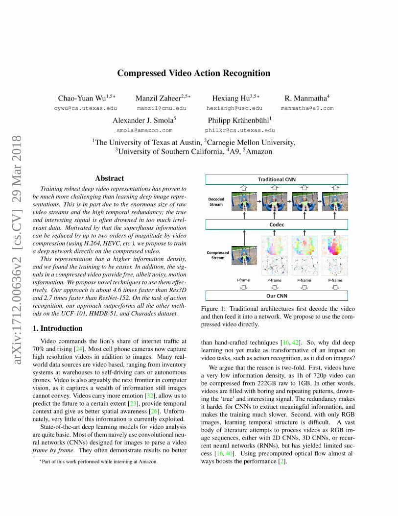
Figure 1: Traditional architectures first decode the videoand then feed it into a network. We propose to use the com-pressed video directly.

than hand-crafted techniques [16, 42]. So, why did deeplearning not yet make as transformative of an impact onvideo tasks, such as action recognition, as it did on images?

We argue that the reason is two-fold. First, videos havea very low information density, as 1h of 720p video canbe compressed from 222GB raw to 1GB. In other words,videos are filled with boring and repeating patterns, drown-ing the ‘true’ and interesting signal. The redundancy makesit harder for CNNs to extract meaningful information, andmakes the training much slower. Second, with only RGBimages, learning temporal structure is difficult. A vastbody of literature attempts to process videos as RGB im-age sequences, either with 2D CNNs, 3D CNNs, or recur-rent neural networks (RNNs), but has yielded limited suc-cess [16, 40]. Using precomputed optical flow almost al-ways boosts the performance [2].

arX

iv:1

712.

0063

6v2

[cs

.CV

] 2

9 M

ar 2

018

To address these issues, we exploit the compressedrepresentation developed for storage and transmission ofvideos rather than operating on the RGB frames (Figure 1).These compression techniques (like MPEG-4, H.264 etc.)leverage that successive frames are usually similar. Theyretain only a few frames completely and reconstruct otherframes based on offsets, called motion vectors and resid-ual error, from the complete images. Our model consists ofmultiple CNNs that directly operate on the motion vectors,residuals, in addition to a small number of complete images.

Why is this better? First, video compression removesup to two orders of magnitude of superfluous information,making interesting signals prominent. Second, the motionvectors in video compression provide us the motion infor-mation that lone RGB images do not have. Furthermore,the motion signals already exclude spatial variations, e.g.two people performing the same action in different cloth-ings or in different lighting conditions exhibit the same mo-tion signals. This improves generalization, and the loweredvariance further simplifies training. Third, with compressedvideo, we account for correlation in video frames, i.e. spa-tial view plus some small changes over time, instead of i.i.d.images. Constraining data in this structure helps us tacklingthe curse of dimensionality. Last but not least, our method isalso much more efficient as we only look at the true signalsinstead of repeatedly processing near-duplicates. Efficiencyis also gained by avoiding to decompress the video, becausevideo is usually stored or transmitted in the compressed ver-sion, and access to the motion vectors and residuals are free.

On action recognition datasets UCF-101 [34], HMDB-51 [18], and Charades [32], our approach significantly out-performs all other methods that train on traditional RGB im-ages. Our approach is simple and fast, without using RNNs,complicated fusion or 3D convolutions. It is 4.6 times fasterthan state-of-the-art 3D CNN model Res3D [40], and 2.7times faster than ResNet-152 [12]. When combined withscores from a standard temporal stream network, our modeloutperforms state-of-the-art methods on all these datasets.

2. BackgroundIn this section we provide a brief overview about video

action recognition and video compression.

2.1. Action Recognition

Traditionally, for video action recognition, the commu-nity utilized hand-crafted features, such as Histogram ofOriented Gradients (HOG) [3] or Histogram of OpticalFlow (HOF) [19], both sparsely [19] and densely [43] sam-pled. While early methods consider independent interestpoints across frames, smarter aggregation based on densetrajectories have been used [25, 41, 42]. Some of these tra-ditional methods are competitive even today, like iDT whichcorrects for camera motion [42].

In the past few years, deep learning has brought signif-icant improvements to video understanding [6, 16]. How-ever, the improvements mainly stem from improvements indeep image representations. Modeling of temporal structureis still relatively simple — most algorithms subsample a fewframes and perform average pooling to make final predic-tions [33, 44]. RNNs [6, 48], temporal CNNs [21], or otherfeature aggregation techniques [11, 44] on top of CNN fea-tures have also been explored. However, while introducingnew computation overhead, these methods do not necessar-ily outperform simple average pooling [44]. Some worksexplore 3D CNNs to model the temporal structure [39, 40].Nonetheless, it results in an explosion of parameters andcomputation time and only marginally improves the perfor-mance [40].

More importantly, evidence suggests that these methodsare not sufficient to capture all temporal structures — usingof pre-computed optical flow almost always boosts the per-formance [2, 9, 33, 44]. This emphasizes the importance ofusing the right input representation and the inadequacy ofRGB frames. Finally, note that all of these methods requireraw video frame-by-frame and cannot exploit the fact thatvideo is stored in some compressed format.

2.2. Video Compression

The need for efficient video storage and transmission hasled to highly efficient video compression algorithms, suchas MPEG-4, H.264, and HEVC, some of which date backto 1990s [20]. Most video compression algorithms lever-age the fact that successive frames are usually very similar.We can efficiently store one frame by reusing contents fromanother frame and only store the difference.

Most modern codecs split a video into I-frames (intra-coded frames), P-frames (predictive frames) and zero ormore B-frames (bi-directional frames). I-frames are regu-lar images and compressed as such. P-frames reference theprevious frames and encode only the ‘change’. A part ofthe change – termed motion vectors – is represented as themovements of block of pixels from the source frame to thetarget frame at time t, which we denote by T (t). Even afterthis compensation for block movement, there can be differ-ence between the original image and the predicted image attime t. We denote this residual difference by ∆(t). Puttingit together, a P-frame at time t only comprises of motionvectors T (t) and a residual ∆(t). This gives the recurrencerelation for reconstructing P-frames as

I(t)i = I

(t−1)i−T (t)

i

+ ∆(t)i , (1)

for all pixel i, where I(t) denotes the RGB image at timet. The motion vectors and the residuals are then passedthrough discrete cosine transform (DCT) and entropy-encoded.

P-frame

t=1t=4t=7t=10

Motionvectors

Accumulatedmotionvectors

Residual

Accumulatedresidual

Figure 2: Original motion vectors and residuals describeonly the change between two frames. Usually the signalto noise ratio is very low and hard to model. The accu-mulated motion vectors and residuals consider longer termdifference and show clearer patterns. Assume I-frame is att = 0. Motion vectors are plotted in HSV space, where theH channel encodes the direction of motion, and the S chan-nel shows the amplitude. For residuals we plot the absolutevalues in RGB space. Best viewed in color.

A B-frame may be viewed as a special P-frame, wheremotion vectors are computed bi-directionally and may ref-erence a future frame as long as there are no circles in ref-erencing. Both B- and P- frames capture only what changesin the video, and are easier to compress owing to smallerdynamic range [28]. See Figure 2 for a visualization of themotion estimates and the residuals. Modeling arbitrary de-coding order is beyond the scope of this paper. We focus onvideos encoded using only backward references, namely I-and P- frames.

Features from Compressed Data. Some prior workshave utilized signals from compressed video for detection orrecognition, but only as a non-deep feature [15, 36, 38, 47].To the best of our knowledge, this is the first work that con-siders training deep networks on compressed videos. MV-CNN apply distillation to transfer knowledge from an opti-cal flow network to a motion vector network [50]. However,unlike our approach, it does not consider the general settingof representation learning on a compressed video; it stillneeds the entire decompressed video as RGB stream, and itrequires optical flow as an additional supervision.

Equipped with this background, next we will explorehow to utilize the compressed representation, devoid of re-dundant information, for action recognition.

� � � �

t=1 t=2 t=3 t=4 t=4

Figure 3: We trace all motion vectors back to the referenceI-frame and accumulate the residual. Now each P-framedepends only on the I-frame but not other P-frames.

3. Modeling Compressed RepresentationsOur goal is to design a computer vision system for action

recognition that operates directly on the stored compressedvideo. The compression is solely designed to optimize thesize of the encoding, thus the resulting representation hasvery different statistical and structural properties than theimages in a raw video. It is not clear if the successful deeplearning techniques can be adapted to compressed represen-tations in a straightforward manner. So we ask how to feeda compressed video into a computer vision system, specifi-cally a deep network?

Feeding I-frames into a deep network is straightforwardsince they are just images. How about P-frames? From Fig-ure 2 we can see that motion vectors, though noisy, roughlyresemble optical flows. As modeling optical flows withCNNs has been proven effective, it is tempting to do thesame for motion vectors. The third row of Figure 2 visu-alizes the residuals. We can see that they roughly give usa motion boundary in addition to a change of appearance,such as the change of lighting conditions. Again, CNNs arewell-suited for such patterns. The outputs of correspondingCNNs from the image, motion vectors, and residual willhave different properties. To combine them, we tried var-ious fusion strategies, including mean pooling, maximumpooling, concatenation, convolution pooling, and bilinearpooling, on both middle layers and the final layer, but withlimited success.

Digging deeper, one can argue that the motion vectorsand residuals alone do not contain the full information ofa P-frame — a P-frame depends on the reference frame,which again might be a P-frame. This chain continues allthe way back to a preceding I-frame. Treating each P-frameas an independent observation clearly violates this depen-dency. A simple strategy to address this is to reuse featuresfrom the reference frame, and only update the features giventhe new information. This recurrent definition screams forRNNs to aggregate features along the chain. However, pre-liminary experiments suggest the elaborate modeling effortin vain (see supplementary material for details). The dif-ficulty arises from the long chain of dependency of the P-frames. To mitigate this issue, we devise a novel yet simpleback-tracing technique that decouples individual P-frames.

…

…

I-frame P-frame

(a) Original dependency.

…

…

I-frame P-frame

(b) New dependency.

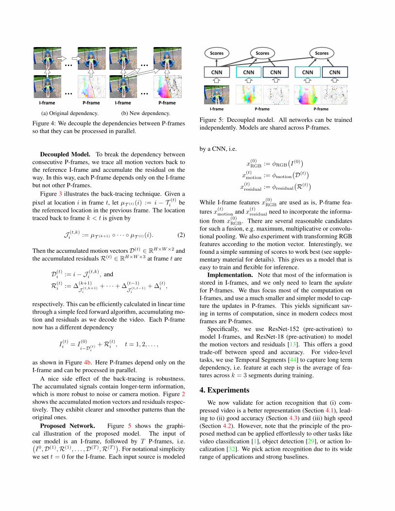
Figure 4: We decouple the dependencies between P-framesso that they can be processed in parallel.

Decoupled Model. To break the dependency betweenconsecutive P-frames, we trace all motion vectors back tothe reference I-frame and accumulate the residual on theway. In this way, each P-frame depends only on the I-framebut not other P-frames.

Figure 3 illustrates the back-tracing technique. Given apixel at location i in frame t, let µT (t)(i) := i − T (t)

i bethe referenced location in the previous frame. The locationtraced back to frame k < t is given by

J (t,k)i := µT (k+1) ◦ · · · ◦ µT (t)(i). (2)

Then the accumulated motion vectorsD(t) ∈ RH×W×2 andthe accumulated residualsR(t) ∈ RH×W×3 at frame t are

D(t)i := i− J (t,k)

i , and

R(t)i := ∆

(k+1)

J (t,k+1)i

+ · · ·+ ∆(t−1)J (t,t−1)

i

+ ∆(t)i ,

respectively. This can be efficiently calculated in linear timethrough a simple feed forward algorithm, accumulating mo-tion and residuals as we decode the video. Each P-framenow has a different dependency

I(t)i = I

(0)

i−D(t)i

+R(t)i , t = 1, 2, . . . ,

as shown in Figure 4b. Here P-frames depend only on theI-frame and can be processed in parallel.

A nice side effect of the back-tracing is robustness.The accumulated signals contain longer-term information,which is more robust to noise or camera motion. Figure 2shows the accumulated motion vectors and residuals respec-tively. They exhibit clearer and smoother patterns than theoriginal ones.

Proposed Network. Figure 5 shows the graphi-cal illustration of the proposed model. The input ofour model is an I-frame, followed by T P-frames, i.e.(I0,D(1),R(1), . . . ,D(T ),R(T )

). For notational simplicity

we set t = 0 for the I-frame. Each input source is modeled

ScoresScores Scores

CNN CNN CNN CNNCNN

I-frame P-frame P-frame

Figure 5: Decoupled model. All networks can be trainedindependently. Models are shared across P-frames.

by a CNN, i.e.

x(0)RGB := φRGB

(I(0)

)x(t)motion := φmotion

(D(t)

)x(t)residual := φresidual

(R(t)

)While I-frame features x(0)RGB are used as is, P-frame fea-tures x(t)motion and x(t)residual need to incorporate the informa-tion from x

(0)RGB. There are several reasonable candidates

for such a fusion, e.g. maximum, multiplicative or convolu-tional pooling. We also experiment with transforming RGBfeatures according to the motion vector. Interestingly, wefound a simple summing of scores to work best (see supple-mentary material for details). This gives us a model that iseasy to train and flexible for inference.

Implementation. Note that most of the information isstored in I-frames, and we only need to learn the updatefor P-frames. We thus focus most of the computation onI-frames, and use a much smaller and simpler model to cap-ture the updates in P-frames. This yields significant sav-ing in terms of computation, since in modern codecs mostframes are P-frames.

Specifically, we use ResNet-152 (pre-activation) tomodel I-frames, and ResNet-18 (pre-activation) to modelthe motion vectors and residuals [13]. This offers a goodtrade-off between speed and accuracy. For video-leveltasks, we use Temporal Segments [44] to capture long termdependency, i.e. feature at each step is the average of fea-tures across k = 3 segments during training.

4. ExperimentsWe now validate for action recognition that (i) com-

pressed video is a better representation (Section 4.1), lead-ing to (ii) good accuracy (Section 4.3) and (iii) high speed(Section 4.2). However, note that the principle of the pro-posed method can be applied effortlessly to other tasks likevideo classification [1], object detection [29], or action lo-calization [32]. We pick action recognition due to its widerange of applications and strong baselines.

Datasets and Protocol. We evaluate our method Com-pressed Video Action Recognition (CoViAR) on three ac-tion recognition datasets, UCF-101 [34], HMDB-51 [18],and Charades [32]. UCF-101 and HMDB-51 contain short(< 10-second) trimmed videos, each of which is annotatedwith one action label. Charades contains longer (∼ 30-second) untrimmed videos. Each video is annotated withone or more action labels and their intervals (start time, endtime). UCF-101 contains 13,320 videos from 101 actioncategories. HMDB-51 contains 6,766 videos from 51 ac-tion categories. Each dataset has 3 (training, testing)-splits.We report the average performance of the 3 testing splits un-less otherwise stated. The Charades dataset contains 9,848videos split into 7,985 training and 1,863 test videos. Itcontains 157 action classes.

During testing we uniformly sample 25 frames, eachwith flips plus 5 crops, and then average the scores for fi-nal prediction. On UCF-101 and HMDB-51 we use tem-poral segments, and perform the averaging before softmaxfollowing TSN [44]. On Charades we use mean averageprecision (mAP) and weighted average precision (wAP) toevaluate the performance, following previous work [31].

Training Details. Following TSN [44], we resize UCF-101 and HMDB-51 videos to 340× 256. As Charades con-tains both portrait and landscape videos, we resize them to256 × 256. Our models are pre-trained on the ILSVRC2012-CLS dataset [4], and fine-tuned using Adam [17] witha batch size of 40. Learning rate starts from 0.001 for UCF-101/HMDB-51 and 0.03 for Charades. It is divided by 10when the accuracy plateaus. Pre-trained layers use a 100×smaller learning rate. We apply color jittering and ran-dom cropping to 224×224 for data augmentation followingTSN [44]. Where available, we select the hyper-parameterson splits other than the tested one. We use MPEG-4 en-coded videos, which have on average 11 P-frames for everyI-frame. Optical flow models use TV-L1 flows [49].

4.1. Ablation StudyHere we study the benefits of using compressed repre-

sentations over RGB images. We focus on UCF-101 andHMDB-51, as they are two of the most well-studied actionrecognition datasets. Table 1 presents a detailed analysis.On both datasets, training on compressed videos signifi-cantly outperforms training on RGB frames. In particular, itprovides 5.8% and 2.7% absolute improvement on HMDB-51 and UCF-101 respectively.

Quite surprisingly, while residuals contribute to a verysmall amount of data, it alone achieves good accuracy. Mo-tion vectors alone perform not as well, as they do not con-tain spatial details. However, they offer information orthog-onal to what still images provide. When added to otherstreams, it significantly boosts the performance. Note thatwe use only I-frames as full images, which is a small subsetof all frames, yet CoViAR achieves good performance.

I M R I+M I+R I+M+R (gain)

UCF-101Split 1 88.4 63.9 79.9 90.4 90.0 90.8 (+2.4)Split 2 87.4 64.6 80.8 89.9 89.6 90.5 (+3.1)Split 3 87.3 66.6 82.1 89.6 89.4 90.0 (+2.7)Average 87.7 65.0 80.9 89.9 89.7 90.4 (+2.7)

HMDB-51Split 1 54.1 37.8 44.6 60.3 55.9 60.4 (+6.3)Split 2 51.9 38.7 43.1 57.9 54.2 58.2 (+6.3)Split 3 54.1 39.7 44.4 58.5 55.6 58.7 (+4.6)Average 53.3 38.8 44.1 58.9 55.2 59.1 (+5.8)

Table 1: Action recognition accuracy on UFC-101 [34] andHMDB-51 [18]. Here we compare training with differentsources of information. “+” denotes score fusion of mod-els. I: I-frame RGB image. M: motion vectors. R: residu-als. The bold numbers indicate the best and the underlinednumbers indicate the second best performance.

M R I+M I+R I+M+R

Original 58.3 79.0 90.0 89.8 90.4Accumulated 63.9 79.9 90.4 90.0 90.8

Table 2: Action recognition accuracy on UFC-101 [34](Split 1). The two rows show the performance of the modelstrained using the original motion vectors/residuals and themodels using the accumulated ones respectively. I: I-frameRGB image. M: motion vectors. R: residuals.

Accumulated Motion Vectors and Residuals. Ourback-tracing technique not only simplifies the dependencybut also results in clearer patterns to model. This improvesthe performance, as shown in Table 2. On the first split ofUCF-101, our accumulation technique provides 5.6% im-provement on the motion vector stream network and onthe full model, 0.4% improvement (4.2% error reduction).Performance of the residual stream also improves by 0.9%(4.3% error reduction).

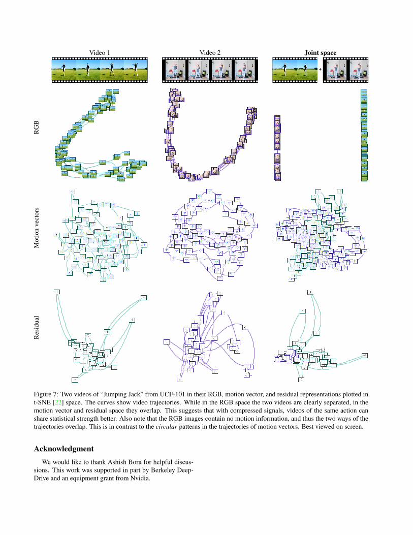
Visualizations. In Figure 7, we qualitatively study theRGB and compressed representations of two videos of thesame action in t-SNE [22] space. We can see that in RGBspace the two videos are clearly separated, and in motionvector and residual space they overlap. This suggests thata RGB-image based model needs to learn the two patternsseparately, while a compressed-video based model sees ashared representation for videos of the same action, makingtraining and generalization easier.

In addition, note that the two ways of the RGB trajecto-ries overlap, showing that RGB images cannot distinguishbetween the up-moving and down-moving motion. On theother hand, compressed signals preserve motion. The tra-jectories thus form circles instead of going back and forthon the same path.

Accuracy (%)GFLOPs UCF-101 HMDB-51

ResNet-50 [8] 3.8 82.3 48.9ResNet-152 [8] 11.3 83.4 46.7C3D [39] 38.5 82.3 51.6Res3D [40] 19.3 85.8 54.9CoViAR 4.2 90.4 59.1

Table 3: Network computation complexity and accuracy ofeach method. Our method is 4.6x more efficient than state-of-the-art 3D CNN, while being much more accurate.

Preprocess CNN CNN(sequential) (concurrent)

Two-streamBN-Inception 75.0 1.6 0.9ResNet-152 75.0 7.5 4.0

CoViAR 2.87/0.46 1.3 0.3

Table 4: Speed (ms) per frame. CoViAR is fast in both pre-processing and CNN computation. Its preprocessing speedis presented for both single-thread / multi-thread settings.

4.2. Speed and Efficiency

Our method is efficient because the computation on theI-frame is shared across multiple frames, and the compu-tation on P-frames is cheaper. Table 3 compares the CNNcomputational cost of our method with state-of-the-art 2Dand 3D CNN architectures. Since for our model the P-and I-frame computational costs are different, we report theaverage GFLOPs over all frames. As shown in the table,CoViAR is 2.7 times faster than ResNet-152 [12] and is 4.6times more than Res3D [40], while being significantly moreaccurate.

A more detailed speed analysis is presented in Table 4.The preprocessing time of the two-stream methods, i.e. op-tical flow computation, is measured on a Tesla P100 GPUwith an implementation of the TV-L1 flow algorithm fromOpenCV. Our preprocessing, i.e. the calculation of the ac-cumulated motion vectors and residuals, is measured on In-tel E5-2698 v4 CPUs. CNN time is measured on the sameP100 GPU. We can see that the optical flow computationis the bottleneck for two-stream networks, even with low-resolution 256 × 340 videos. Our preprocessing is muchfaster despite our CPU-only implementation.

For CNN time, we consider both settings where (i) wecan forward multiple CNNs at the same time, and (ii) we doit sequentially. For both settings, our method is significantlyfaster than traditional methods. Overall, our method can beup to 100 times faster than traditional methods with multi-thread preprocessing, running at 1,300 frames per second.Figure 6 summarizes the results. CoViAR achieves the bestefficiency and good accuracy, while requiring a far lesseramount of data.

100 101 102

60

80

100

Compressedvideo

RGB RGB+Flows

Two-stream

Res3D

ResNet-152

CoViAR

Inference time (ms per frame)

Acc

urac

y

Figure 6: Speed and accuracy on UCF-101 [34], comparedto a two-stream network (TSN) [33, 44], Res3D [40], andResNet-152 [12] trained on RGB frames. Node size denotesthe input data size. Training on compressed videos is bothaccurate and efficient.

UCF-101 HMDB-51CoViAR Flow CoViAR CoViAR Flow CoViAR

+flow +flow

Split 1 90.8 87.7 94.0 60.4 61.8 71.5Split 2 90.5 90.2 95.4 58.2 63.7 69.4Split 3 90.0 89.1 95.2 58.7 64.2 69.7Average 90.4 89.0 94.9 59.1 63.2 70.2

Table 5: Action recognition accuracy on UFC-101 [34] andHMDB-51 [18]. Combining our model with a temporal-stream network achieves state-of-the-art performance.

4.3. Accuracy

We now compare the accuracy of CoViAR with state-of-the-art models in Table 6. For fair comparison, here we fo-cus on models using the same pre-training dataset, ILSVRC2012-CLS [4]. While pre-training using Kinetics yields bet-ter performance [2], since it is larger and more similar tothe datasets used in this paper, those results are not directlycomparable.

From the upper part of the table, we can see thatour model significantly outperforms traditional RGB-imagebased methods. C3D [39], Res3D [40], P3D ResNet [27],and I3D [2] consider 3D convolution to learn temporalstructures. Karpathy et al. [16] and TLE [5] consider morecomplicated fusions and pooling. MV-CNN [50] apply dis-tillation to transfer knowledge from an optical-flow-basedmodel. Our method uses much faster 2D CNNs plus simplelate fusion without additional supervision, and still signifi-cantly outperforms these methods.

†Despite our best efforts, we were not able to reproduce the perfor-mance reported in the original paper. Here we report the performancebased on our implementation. For fair comparison, we use the same dataaugmentation and architecture as ours. Training follows the 2-stage pro-

UCF-101 HMDB-51

Without optical flowKarpathy et al. [16] 65.4 -ResNet-50 [12] (from ST-Mult [8]) 82.3 48.9ResNet-152 [12] (from ST-Mult [8]) 83.4 46.7C3D [39] 82.3 51.6Res3D [40] 85.8 54.9TSN (RGB-only) [44]* 85.7 -TLE (RGB-only) [5]† 87.9 54.2I3D (RGB-only) [2]* 84.5 49.8MV-CNN [50] 86.4 -P3D ResNet [27] 88.6 -Attentional Pooling [10] - 52.2CoViAR 90.4 59.1

With optical flowiDT+FV [42] - 57.2Two-Stream [33] 88.0 59.4Two-Stream fusion [9] 92.5 65.4LRCN [6] 82.7Composite LSTM Model [35] 84.3 44.0ActionVLAD [11] 92.7 66.9ST-ResNet [7] 93.4 66.4ST-Mult [8] 94.2 68.9I3D [2]* 93.4 66.4TLE [5]† 93.8 68.8L2STM [37] 93.6 66.2ShuttleNet [30] 94.4 66.6STPN [45] 94.6 68.9TSN [44] 94.2 69.4CoViAR + optical flow 94.9 70.2

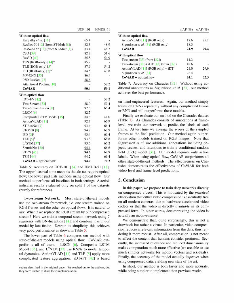
Table 6: Accuracy on UCF-101 [34] and HMDB-51 [18].The upper lists real-time methods that do not require opticalflow; the lower part lists methods using optical flow. Ourmethod outperforms all baselines in both settings. Asteriskindicates results evaluated only on split 1 of the datasets(purely for reference).

Two-stream Network. Most state-of-the-art modelsuse the two-stream framework, i.e. one stream trained onRGB frames and the other on optical flows. It is natural toask: What if we replace the RGB stream by our compressedstream? Here we train a temporal-stream network using 7segments with BN-Inception [14], and combine it with ourmodel by late fusion. Despite its simplicity, this achievesvery good performance as shown in Table 5.

The lower part of Table 6 compares our method withstate-of-the-art models using optical flow. CoViAR out-performs all of them. LRCN [6], Composite LSTMModel [35], and L2STM [37] use RNNs to model tempo-ral dynamics. ActionVLAD [11] and TLE [5] apply morecomplicated feature aggregation. iDT+FT [42] is based

cedure described in the original paper. We reached out to the authors, butthey were unable to share their implementation.

mAP (%) wAP (%)

Without optical flowActionVLAD [11] (RGB only) 17.6 25.1Sigurdsson et al. [31] (RGB only) 18.3 -CoViAR 21.9 29.4

With optical flowTwo-stream [33] (from [32]) 14.3 -Two-stream [33] + iDT [42] (from [32]) 18.6 -ActionVLAD [11] (RGB only) + iDT 21.0 29.9Sigurdsson et al. [31] 22.4 -CoViAR + optical flow 24.1 32.3

Table 7: Accuracy on Charades [32]. Without using ad-ditional annotations as Sigurdsson et al. [31], our methodachieves the best performance.

on hand-engineered features. Again, our method simplytrains 2D CNNs separately without any complicated fusionor RNN and still outperforms these models.

Finally we evaluate our method on the Charades dataset(Table 7). As Charades consists of annotations at frame-level, we train our network to predict the labels of eachframe. At test time we average the scores of the sampledframes as the final prediction. Our method again outper-forms other models trained on RGB images. Note thatSigurdsson et al. use additional annotations including ob-jects, scenes, and intentions to train a conditional randomfield (CRF) model [31]. Our model requires only actionlabels. When using optical flow, CoViAR outperforms allother state-of-the-art methods. The effectiveness on Cha-rades demonstrates the effectiveness of CoViAR for bothvideo-level and frame-level predictions.

5. Conclusion

In this paper, we propose to train deep networks directlyon compressed videos. This is motivated by the practicalobservation that either video compression is essentially freeon all modern cameras, due to hardware-accelerated videocodecs or that the video is directly available in its com-pressed form. In other words, decompressing the video isactually an inconvenience.

We demonstrate that, quite surprisingly, this is not adrawback but rather a virtue. In particular, video compres-sion reduces irrelevant information from the data, thus ren-dering it more robust. After all, compression is not meantto affect the content that humans consider pertinent. Sec-ondly, the increased relevance and reduced dimensionalitymakes computation much more effective (we are able to usemuch simpler networks for motion vectors and residuals).Finally, the accuracy of the model actually improves whenusing compressed data, yielding new state of the art.

In short, our method is both faster and more accurate,while being simpler to implement than previous works.

Video 1 Video 2 Joint space

+

RG

BM

otio

nve

ctor

sR

esid

ual

Figure 7: Two videos of “Jumping Jack” from UCF-101 in their RGB, motion vector, and residual representations plotted int-SNE [22] space. The curves show video trajectories. While in the RGB space the two videos are clearly separated, in themotion vector and residual space they overlap. This suggests that with compressed signals, videos of the same action canshare statistical strength better. Also note that the RGB images contain no motion information, and thus the two ways of thetrajectories overlap. This is in contrast to the circular patterns in the trajectories of motion vectors. Best viewed on screen.

AcknowledgmentWe would like to thank Ashish Bora for helpful discus-

sions. This work was supported in part by Berkeley Deep-Drive and an equipment grant from Nvidia.

References[1] S. Abu-El-Haija, N. Kothari, J. Lee, P. Natsev, G. Toderici,

B. Varadarajan, and S. Vijayanarasimhan. YouTube-8M: Alarge-scale video classification benchmark. arXiv preprintarXiv:1609.08675, 2016. 4

[2] J. Carreira and A. Zisserman. Quo vadis, action recognition?a new model and the kinetics dataset. In CVPR, 2017. 1, 2,6, 7

[3] N. Dalal and B. Triggs. Histograms of oriented gradients forhuman detection. In CVPR, 2005. 2

[4] J. Deng, W. Dong, R. Socher, L.-J. Li, K. Li, and L. Fei-Fei. ImageNet: A large-scale hierarchical image database.In CVPR, 2009. 5, 6

[5] A. Diba, V. Sharma, and L. Van Gool. Deep temporal linearencoding networks. CVPR, 2017. 6, 7

[6] J. Donahue, L. Anne Hendricks, S. Guadarrama,M. Rohrbach, S. Venugopalan, K. Saenko, and T. Dar-rell. Long-term recurrent convolutional networks for visualrecognition and description. In CVPR, 2015. 2, 7

[7] C. Feichtenhofer, A. Pinz, and R. Wildes. Spatiotemporalresidual networks for video action recognition. In NIPS,2016. 7

[8] C. Feichtenhofer, A. Pinz, and R. P. Wildes. Spatiotemporalmultiplier networks for video action recognition. In CVPR,2017. 6, 7, 11

[9] C. Feichtenhofer, A. Pinz, and A. Zisserman. Convolutionaltwo-stream network fusion for video action recognition. InCVPR, 2016. 2, 7

[10] R. Girdhar and D. Ramanan. Attentional pooling for actionrecognition. In NIPS, 2017. 7

[11] R. Girdhar, D. Ramanan, A. Gupta, J. Sivic, and B. Russell.Actionvlad: Learning spatio-temporal aggregation for actionclassification. In CVPR, 2017. 2, 7

[12] K. He, X. Zhang, S. Ren, and J. Sun. Deep residual learningfor image recognition. In CVPR, 2016. 2, 6, 7

[13] K. He, X. Zhang, S. Ren, and J. Sun. Identity mappings indeep residual networks. In ECCV, 2016. 4

[14] S. Ioffe and C. Szegedy. Batch normalization: Acceleratingdeep network training by reducing internal covariate shift. InICML, 2015. 7

[15] V. Kantorov and I. Laptev. Efficient feature extraction, en-coding and classification for action recognition. In CVPR,2014. 3

[16] A. Karpathy, G. Toderici, S. Shetty, T. Leung, R. Sukthankar,and L. Fei-Fei. Large-scale video classification with convo-lutional neural networks. In CVPR, 2014. 1, 2, 6, 7

[17] D. Kingma and J. Ba. Adam: A method for stochastic opti-mization. arXiv preprint arXiv:1412.6980, 2014. 5

[18] H. Kuehne, H. Jhuang, E. Garrote, T. Poggio, and T. Serre.HMDB: a large video database for human motion recogni-tion. In ICCV, 2011. 2, 5, 6, 7

[19] I. Laptev, M. Marszalek, C. Schmid, and B. Rozenfeld.Learning realistic human actions from movies. In CVPR,2008. 2

[20] D. Le Gall. Mpeg: A video compression standard for multi-media applications. Communications of the ACM, 1991. 2

[21] C.-Y. Ma, M.-H. Chen, Z. Kira, and G. AlRegib. TS-LSTM and temporal-inception: Exploiting spatiotempo-ral dynamics for activity recognition. arXiv preprintarXiv:1703.10667, 2017. 2

[22] L. v. d. Maaten and G. Hinton. Visualizing data using t-SNE.JMLR, 2008. 5, 8

[23] M. Mathieu, C. Couprie, and Y. LeCun. Deep multi-scalevideo prediction beyond mean square error. ICLR, 2016. 1

[24] C. V. networking Index. Forecast and methodology, 2016-2021, white paper. San Jose, CA, USA, 2016. 1

[25] X. Peng, C. Zou, Y. Qiao, and Q. Peng. Action recognitionwith stacked fisher vectors. In ECCV, 2014. 2

[26] M. Pollefeys, D. Nister, J.-M. Frahm, A. Akbarzadeh,P. Mordohai, B. Clipp, C. Engels, D. Gallup, S.-J. Kim,P. Merrell, et al. Detailed real-time urban 3d reconstructionfrom video. IJCV, 2008. 1

[27] Z. Qiu, T. Yao, and T. Mei. Learning spatio-temporal repre-sentation with pseudo-3d residual networks. In ICCV, 2017.6, 7

[28] I. E. Richardson. Video codec design: developing image andvideo compression systems. John Wiley & Sons, 2002. 3

[29] O. Russakovsky, J. Deng, H. Su, J. Krause, S. Satheesh,S. Ma, Z. Huang, A. Karpathy, A. Khosla, M. Bernstein,A. C. Berg, and L. Fei-Fei. ImageNet large scale visualrecognition challenge. IJCV, 2015. 4

[30] Y. Shi, Y. Tian, Y. Wang, W. Zeng, and T. Huang. Learn-ing long-term dependencies for action recognition with abiologically-inspired deep network. In ICCV, 2017. 7

[31] G. A. Sigurdsson, S. Divvala, A. Farhadi, and A. Gupta.Asynchronous temporal fields for action recognition. InCVPR, 2017. 5, 7

[32] G. A. Sigurdsson, G. Varol, X. Wang, A. Farhadi, I. Laptev,and A. Gupta. Hollywood in homes: Crowdsourcing datacollection for activity understanding. In ECCV, 2016. 1, 2,4, 5, 7

[33] K. Simonyan and A. Zisserman. Two-stream convolutionalnetworks for action recognition in videos. In NIPS, 2014. 2,6, 7

[34] K. Soomro, A. Roshan Zamir, and M. Shah. UCF101: Adataset of 101 human actions classes from videos in the wild.In CRCV-TR-12-01, 2012. 2, 5, 6, 7

[35] N. Srivastava, E. Mansimov, and R. Salakhudinov. Unsuper-vised learning of video representations using lstms. In ICML,2015. 7

[36] O. Sukmarg and K. R. Rao. Fast object detection and seg-mentation in MPEG compressed domain. In TENCON, 2000.3

[37] L. Sun, K. Jia, K. Chen, D.-Y. Yeung, B. E. Shi, andS. Savarese. Lattice long short-term memory for human ac-tion recognition. In ICCV, 2017. 7

[38] B. U. Toreyin, A. E. Cetin, A. Aksay, and M. B. Akhan.Moving object detection in wavelet compressed video. Sig-nal Processing: Image Communication, 2005. 3

[39] D. Tran, L. Bourdev, R. Fergus, L. Torresani, and M. Paluri.Learning spatiotemporal features with 3d convolutional net-works. In ICCV, 2015. 2, 6, 7

[40] D. Tran, J. Ray, Z. Shou, S.-F. Chang, and M. Paluri. Con-vNet architecture search for spatiotemporal feature learning.arXiv preprint arXiv:1708.05038, 2017. 1, 2, 6, 7, 11

[41] H. Wang, A. Klaser, C. Schmid, and C.-L. Liu. Dense tra-jectories and motion boundary descriptors for action recog-nition. IJCV, 2013. 2

[42] H. Wang and C. Schmid. Action recognition with improvedtrajectories. In ICCV, 2013. 1, 2, 7

[43] H. Wang, M. M. Ullah, A. Klaser, I. Laptev, and C. Schmid.Evaluation of local spatio-temporal features for action recog-nition. In BMVC, 2009. 2

[44] L. Wang, Y. Xiong, Z. Wang, Y. Qiao, D. Lin, X. Tang, andL. Van Gool. Temporal segment networks: Towards goodpractices for deep action recognition. In ECCV, 2016. 2, 4,5, 6, 7, 11

[45] Y. Wang, M. Long, J. Wang, and P. S. Yu. Spatiotempo-ral pyramid network for video action recognition. In CVPR,2017. 7

[46] S. Xingjian, Z. Chen, H. Wang, D.-Y. Yeung, W.-K. Wong,and W.-c. Woo. Convolutional LSTM network: A machinelearning approach for precipitation nowcasting. In NIPS,2015. 11

[47] B.-L. Yeo and B. Liu. Rapid scene analysis on compressedvideo. IEEE Transactions on circuits and systems for videotechnology, 1995. 3

[48] J. Yue-Hei Ng, M. Hausknecht, S. Vijayanarasimhan,O. Vinyals, R. Monga, and G. Toderici. Beyond short snip-pets: Deep networks for video classification. In CVPR, 2015.2

[49] C. Zach, T. Pock, and H. Bischof. A duality based approachfor realtime tv-l 1 optical flow. Pattern Recognition, 2007. 5

[50] B. Zhang, L. Wang, Z. Wang, Y. Qiao, and H. Wang. Real-time action recognition with enhanced motion vector CNNs.In CVPR, 2016. 3, 6, 7

Appendix A. RNN-Based Models

Given the recurrent definition of P-frames, one can usea RNN to model a compressed video. In preliminaryexperiments, we experiment with a variant using Conv-LSTMs [46].

The architecture is identical to CoViAR except that i) ituses the original T and ∆ instead of the accumulated Dand R, because here we want to the original dependency,and ii) it uses a Conv-LSTM to aggregate the CNN fea-tures instead of average pooling. Formally, let x(t)fusion :=

max(x(t)motion, x

(t)residual

)denote the max-pooled P-frame

feature at time t. The Conv-LSTM takes the input sequence(x(0)RGB, x

(1)fusion, x

(2)fusion, . . .

).

Here the number of channels of x(0)RGB is reduced from 2048to 512 by an 1 × 1 convolution so that its dimensionalitymatches x(t)fusion. We use 512-dimensional hidden states and3 × 3 kernels for the Conv-LSTM. Due to memory con-straint, we subsample one every two P-frames to reduce thesequence length.

Table 8 presents the results. Even though the Conv-LSTM model outperforms traditional RGB-based methods,the decoupled CoViAR achieves the best performance. Wealso try adding the input of Conv-LSTM to its output as askip connection, but it leads to worse performance (Conv-LSTM-Skip).

RGB-only Conv-LSTM Conv-LSTM-Skip CoViAR

88.4 89.1 87.8 90.8

Table 8: Accuracy on UCF-101 split 1. CoViAR decouplesthe long dependency and outperforms RNN-based models.

Appendix B. Feature Fusion

We experiment with different ways of combining P-frame features, x(t)motion, x(t)residual, and I-frame featuresx(0)RGB. In particular, we evaluate maximum, mean, and mul-

tiplicative fusion, concatenation of feature maps, and latefusion (summing softmax scores). For maximum, mean,and multiplicative fusion, we perform 1× 1 convolution onI-frame feature maps before fusion, so that their dimension-ality matches P-frame features.

Table 9 summarizes the results; we found late fusionworks the best for CoViAR. Note that late fusion allowstraining of a decoupled model, while the rest requires train-ing multiple CNNs jointly. The ease of training of late fu-sion may also contribute to its superior performance.

Max Mean Mult Concat Late

87.9 88.1 87.8 89.7 90.8

Table 9: Accuracy on UCF-101 split 1 with different featurefusion methods.

Appendix C. CoViAR without Temporal Seg-ments

For further analysis, we also evaluate CoViAR withoutusing temporal segments [44] (Table 10). It still signifi-cantly outperforms models using RGB images only, includ-ing ResNet-152 (83.4% in ST-Mult [8]; 84.7% with out im-plementation) and Res3D [40] (85.8%).

I M R I+M I+R I+M+R

84.7 63.4 76.6 87.9 87.2 88.9Table 10: Accuracy of CoViAR without temporal segmentson UFC-101 split 1.

Appendix D. Confusion MatrixFigure 8 and Figure 9 show the confusion matrices of

CoViAR and the model using only RGB images respec-tively, on UCF-101. Figure 10 shows the difference be-tween their predictions. We can see that CoViAR cor-rects many mistakes made by the RGB-based model (off-diagonal purple blocks in Figure 10). For example, whilethe RGB-based model gets confused about the similar ac-tions of Cricket Bowling and Cricket Shot, our model betterdistinguishes between them.

Appl

yEye

Mak

eup

Appl

yLip

stick

Arch

ery

Baby

Craw

ling

Bala

nceB

eam

Band

Mar

chin

gBa

seba

llPitc

hBa

sket

ball

Bask

etba

llDun

kBe

nchP

ress

Biki

ngBi

lliard

sBl

owDr

yHai

rBl

owin

gCan

dles

Body

Wei

ghtS

quat

sBo

wlin

gBo

xing

Punc

hing

Bag

Boxi

ngSp

eedB

agBr

east

Stro

keBr

ushi

ngTe

eth

Clea

nAnd

Jerk

Cliff

Divi

ngCr

icket

Bowl

ing

Crick

etSh

otCu

tting

InKi

tche

nDi

ving

Drum

min

gFe

ncin

gFi

eldH

ocke

yPen

alty

Floo

rGym

nast

icsFr

isbee

Catc

hFr

ontC

rawl

GolfS

wing

Hairc

utHa

mm

erin

gHa

mm

erTh

row

Hand

stan

dPus

hups

Hand

stan

dWal

king

Head

Mas

sage

High

Jum

pHo

rseR

ace

Hors

eRid

ing

Hula

Hoop

IceDa

ncin

gJa

velin

Thro

wJu

gglin

gBal

lsJu

mpi

ngJa

ckJu

mpR

ope

Kaya

king

Knitt

ing

Long

Jum

pLu

nges

Milit

aryP

arad

eM

ixin

gM

oppi

ngFl

oor

Nunc

huck

sPa

ralle

lBar

sPi

zzaT

ossin

gPl

ayin

gCel

loPl

ayin

gDaf

Play

ingD

hol

Play

ingF

lute

Play

ingG

uita

rPl

ayin

gPia

noPl

ayin

gSita

rPl

ayin

gTab

laPl

ayin

gVio

linPo

leVa

ult

Pom

mel

Hors

ePu

llUps

Punc

hPu

shUp

sRa

fting

Rock

Clim

bing

Indo

orRo

peCl

imbi

ngRo

wing

Salsa

Spin

Shav

ingB

eard

Shot

put

Skat

eBoa

rdin

gSk

iing

Skije

tSk

yDiv

ing

Socc

erJu

gglin

gSo

ccer

Pena

ltySt

illRin

gsSu

moW

rest

ling

Surfi

ngSw

ing

Tabl

eTen

nisS

hot

TaiC

hiTe

nnisS

wing

Thro

wDisc

usTr

ampo

lineJ

umpi

ngTy

ping

Unev

enBa

rsVo

lleyb

allS

piki

ngW

alki

ngW

ithDo

gW

allP

ushu

psW

ritin

gOnB

oard

YoYo

Predicted label

ApplyEyeMakeupApplyLipstick

ArcheryBabyCrawlingBalanceBeamBandMarchingBaseballPitch

BasketballBasketballDunk

BenchPressBiking

BilliardsBlowDryHair

BlowingCandlesBodyWeightSquats

BowlingBoxingPunchingBag

BoxingSpeedBagBreastStroke

BrushingTeethCleanAndJerk

CliffDivingCricketBowling

CricketShotCuttingInKitchen

DivingDrumming

FencingFieldHockeyPenalty

FloorGymnasticsFrisbeeCatch

FrontCrawlGolfSwing

HaircutHammering

HammerThrowHandstandPushupsHandstandWalking

HeadMassageHighJump

HorseRaceHorseRiding

HulaHoopIceDancing

JavelinThrowJugglingBallsJumpingJack

JumpRopeKayaking

KnittingLongJump

LungesMilitaryParade

MixingMoppingFloor

NunchucksParallelBars

PizzaTossingPlayingCello

PlayingDafPlayingDholPlayingFlute

PlayingGuitarPlayingPianoPlayingSitar

PlayingTablaPlayingViolin

PoleVaultPommelHorse

PullUpsPunch

PushUpsRafting

RockClimbingIndoorRopeClimbing

RowingSalsaSpin

ShavingBeardShotput

SkateBoardingSkiingSkijet

SkyDivingSoccerJugglingSoccerPenalty

StillRingsSumoWrestling

SurfingSwing

TableTennisShotTaiChi

TennisSwingThrowDiscus

TrampolineJumpingTyping

UnevenBarsVolleyballSpikingWalkingWithDog

WallPushupsWritingOnBoard

YoYo

True

labe

l

0.0

0.2

0.4

0.6

0.8

1.0

Figure 8: Confusion matrix of CoViAR on UCF-101.

Appl

yEye

Mak

eup

Appl

yLip

stick

Arch

ery

Baby

Craw

ling

Bala

nceB

eam

Band

Mar

chin

gBa

seba

llPitc

hBa

sket

ball

Bask

etba

llDun

kBe

nchP

ress

Biki

ngBi

lliard

sBl

owDr

yHai

rBl

owin

gCan

dles

Body

Wei

ghtS

quat

sBo

wlin

gBo

xing

Punc

hing

Bag

Boxi

ngSp

eedB

agBr

east

Stro

keBr

ushi

ngTe

eth

Clea

nAnd

Jerk

Cliff

Divi

ngCr

icket

Bowl

ing

Crick

etSh

otCu

tting

InKi

tche

nDi

ving

Drum

min

gFe

ncin

gFi

eldH

ocke

yPen

alty

Floo

rGym

nast

icsFr

isbee

Catc

hFr

ontC

rawl

GolfS

wing

Hairc

utHa

mm

erin

gHa

mm

erTh

row

Hand

stan

dPus

hups

Hand

stan

dWal

king

Head

Mas

sage

High

Jum

pHo

rseR

ace

Hors

eRid

ing

Hula

Hoop

IceDa

ncin

gJa

velin

Thro

wJu

gglin

gBal

lsJu

mpi

ngJa

ckJu

mpR

ope

Kaya

king

Knitt

ing

Long

Jum

pLu

nges

Milit

aryP

arad

eM

ixin

gM

oppi

ngFl

oor

Nunc

huck

sPa

ralle

lBar

sPi

zzaT

ossin

gPl

ayin

gCel

loPl

ayin

gDaf

Play

ingD

hol

Play

ingF

lute

Play

ingG

uita

rPl

ayin

gPia

noPl

ayin

gSita

rPl

ayin

gTab

laPl

ayin

gVio

linPo

leVa

ult

Pom

mel

Hors

ePu

llUps

Punc

hPu

shUp

sRa

fting

Rock

Clim

bing

Indo

orRo

peCl

imbi

ngRo

wing

Salsa

Spin

Shav

ingB

eard

Shot

put

Skat

eBoa

rdin

gSk

iing

Skije

tSk

yDiv

ing

Socc

erJu

gglin

gSo

ccer

Pena

ltySt

illRin

gsSu

moW

rest

ling

Surfi

ngSw

ing

Tabl

eTen

nisS

hot

TaiC

hiTe

nnisS

wing

Thro

wDisc

usTr

ampo

lineJ

umpi

ngTy

ping

Unev

enBa

rsVo

lleyb

allS

piki

ngW

alki

ngW

ithDo

gW

allP

ushu

psW

ritin

gOnB

oard

YoYo

Predicted label

ApplyEyeMakeupApplyLipstick

ArcheryBabyCrawlingBalanceBeamBandMarchingBaseballPitch

BasketballBasketballDunk

BenchPressBiking

BilliardsBlowDryHair

BlowingCandlesBodyWeightSquats

BowlingBoxingPunchingBag

BoxingSpeedBagBreastStroke

BrushingTeethCleanAndJerk

CliffDivingCricketBowling

CricketShotCuttingInKitchen

DivingDrumming

FencingFieldHockeyPenalty

FloorGymnasticsFrisbeeCatch

FrontCrawlGolfSwing

HaircutHammering

HammerThrowHandstandPushupsHandstandWalking

HeadMassageHighJump

HorseRaceHorseRiding

HulaHoopIceDancing

JavelinThrowJugglingBallsJumpingJack

JumpRopeKayaking

KnittingLongJump

LungesMilitaryParade

MixingMoppingFloor

NunchucksParallelBars

PizzaTossingPlayingCello

PlayingDafPlayingDholPlayingFlute

PlayingGuitarPlayingPianoPlayingSitar

PlayingTablaPlayingViolin

PoleVaultPommelHorse

PullUpsPunch

PushUpsRafting

RockClimbingIndoorRopeClimbing

RowingSalsaSpin

ShavingBeardShotput

SkateBoardingSkiingSkijet

SkyDivingSoccerJugglingSoccerPenalty

StillRingsSumoWrestling

SurfingSwing

TableTennisShotTaiChi

TennisSwingThrowDiscus

TrampolineJumpingTyping

UnevenBarsVolleyballSpikingWalkingWithDog

WallPushupsWritingOnBoard

YoYo

True

labe

l

0.0

0.2

0.4

0.6

0.8

1.0

Figure 9: Confusion matrix of the model using RGB images on UCF-101.

Appl

yEye

Mak

eup

Appl

yLip

stick

Arch

ery

Baby

Craw

ling

Bala

nceB

eam

Band

Mar

chin

gBa

seba

llPitc

hBa

sket

ball

Bask

etba

llDun

kBe

nchP

ress

Biki

ngBi

lliard

sBl

owDr

yHai

rBl

owin

gCan

dles

Body

Wei

ghtS

quat

sBo

wlin

gBo

xing

Punc

hing

Bag

Boxi

ngSp

eedB

agBr

east

Stro

keBr

ushi

ngTe

eth

Clea

nAnd

Jerk

Cliff

Divi

ngCr

icket

Bowl

ing

Crick

etSh

otCu

tting

InKi

tche

nDi

ving

Drum

min

gFe

ncin

gFi

eldH

ocke

yPen

alty

Floo

rGym

nast

icsFr

isbee

Catc

hFr

ontC

rawl

GolfS

wing

Hairc

utHa

mm

erin

gHa

mm

erTh

row

Hand

stan

dPus

hups

Hand

stan

dWal

king

Head

Mas

sage

High

Jum

pHo

rseR

ace

Hors

eRid

ing

Hula

Hoop

IceDa

ncin

gJa

velin

Thro

wJu

gglin

gBal

lsJu

mpi

ngJa

ckJu

mpR

ope

Kaya

king

Knitt

ing

Long

Jum

pLu

nges

Milit

aryP

arad

eM

ixin

gM

oppi

ngFl

oor

Nunc

huck

sPa

ralle

lBar

sPi

zzaT

ossin

gPl

ayin

gCel

loPl

ayin

gDaf

Play

ingD

hol

Play

ingF

lute

Play

ingG

uita

rPl

ayin

gPia

noPl

ayin

gSita

rPl

ayin

gTab

laPl

ayin

gVio

linPo

leVa

ult

Pom

mel

Hors

ePu

llUps

Punc

hPu

shUp

sRa

fting

Rock

Clim

bing

Indo

orRo

peCl

imbi

ngRo

wing

Salsa

Spin

Shav

ingB

eard

Shot

put

Skat

eBoa

rdin

gSk

iing

Skije

tSk

yDiv

ing

Socc

erJu

gglin

gSo

ccer

Pena

ltySt

illRin

gsSu

moW

rest

ling

Surfi

ngSw

ing

Tabl

eTen

nisS

hot

TaiC

hiTe

nnisS

wing

Thro

wDisc

usTr

ampo

lineJ

umpi

ngTy

ping

Unev

enBa

rsVo

lleyb

allS

piki

ngW

alki

ngW

ithDo

gW

allP

ushu

psW

ritin

gOnB

oard

YoYo

Predicted label

ApplyEyeMakeupApplyLipstick

ArcheryBabyCrawlingBalanceBeamBandMarchingBaseballPitch

BasketballBasketballDunk

BenchPressBiking

BilliardsBlowDryHair

BlowingCandlesBodyWeightSquats

BowlingBoxingPunchingBag

BoxingSpeedBagBreastStroke

BrushingTeethCleanAndJerk

CliffDivingCricketBowling

CricketShotCuttingInKitchen

DivingDrumming

FencingFieldHockeyPenalty

FloorGymnasticsFrisbeeCatch

FrontCrawlGolfSwing

HaircutHammering

HammerThrowHandstandPushupsHandstandWalking

HeadMassageHighJump

HorseRaceHorseRiding

HulaHoopIceDancing

JavelinThrowJugglingBallsJumpingJack

JumpRopeKayaking

KnittingLongJump

LungesMilitaryParade

MixingMoppingFloor

NunchucksParallelBars

PizzaTossingPlayingCello

PlayingDafPlayingDholPlayingFlute

PlayingGuitarPlayingPianoPlayingSitar

PlayingTablaPlayingViolin

PoleVaultPommelHorse

PullUpsPunch

PushUpsRafting

RockClimbingIndoorRopeClimbing

RowingSalsaSpin

ShavingBeardShotput

SkateBoardingSkiingSkijet

SkyDivingSoccerJugglingSoccerPenalty

StillRingsSumoWrestling

SurfingSwing

TableTennisShotTaiChi

TennisSwingThrowDiscus

TrampolineJumpingTyping

UnevenBarsVolleyballSpikingWalkingWithDog

WallPushupsWritingOnBoard

YoYo

True

labe

l

30

20

10

0

10

20

30

Figure 10: Difference between CoViAR’s predictions and the RGB-based model’s predictions. For diagonal entries, posi-tive values (in green) is better (increase of correct predictions). For off-diagonal entries, negative values (purple) is better(reduction of wrong predictions).