COMPETITION, MONOPOLY, AND AFTERMARKETS

by

Dennis W. Carlton Graduate School of Business

University of Chicago 1101 East 58th Street Chicago, IL 60637

(773) 702-6694, dennis.carlton@gsb.uchicago.edu

National Bureau of Economic Research, Research Associate

and

Michael Waldman Johnson Graduate School of Management

Cornell University Sage Hall

Ithaca, NY 14853 (607) 255-8631, mw46@cornell.edu

December 2000

4

*We thank Gary Resnick for helpful discussions.

COMPETITION, MONOPOLY, AND AFTERMARKETS

ABSTRACT

Consider a durable goods producer that potentially has market power in the aftermarkets

associated with its products. An important question is to what extent, if any, should the antitrust laws

restrict the firm’s behavior in these aftermarkets? In this paper we explore a number of models

characterized by either competition or monopoly in the new-unit market, and show that a variety of

behaviors that hurt competition in aftermarkets can, in fact, be efficient responses to potential

inefficiencies that can arise in aftermarkets. Our results should give courts pause before intervening in

aftermarkets.

Dennis W. Carlton Graduate School of Business

University of Chicago 1101 East 58th Street Chicago, IL 60637

and

Michael Waldman

Johnson Graduate School of Management Cornell University

2

Sage Hall Ithaca, NY 14853

I. INTRODUCTION

A series of court cases concerning firms such as Kodak, Data General, Unisys, and Xerox,

have focused attention on aftermarkets. The term aftermarkets refers to markets for complementary

goods and services such as maintenance, upgrades, and replacement parts that may be needed after the

consumer has purchased a durable good. A typical allegation is that the durable goods producer

behaves in a fashion that stops alternative producers from offering the complementary good or service

with the result that the original durable goods producer monopolizes the aftermarket. For example, in a

famous 1992 Supreme Court case, Kodak refused to sell spare parts to alternative maintenance

suppliers with the result that consumers of Kodak’s products had no option but to purchase

maintenance from Kodak. In this paper we show that a variety of behaviors that hurt competition in

aftermarkets can, in fact, be efficient responses to potential inefficiencies that can arise in aftermarkets.

Our analysis thus indicates that some courts have likely promoted inefficiency by their antitrust

intervention in aftermarkets.

Our basic argument is that a competitive aftermarket is not necessarily an efficient aftermarket,

and when this is the case the original durable goods producer may behave in a manner that hurts

competition in the aftermarket in order to achieve an efficient outcome. Importantly, there is often

nothing a court can do to improve efficiency that would not be in the interest of the original producer so

court intervention in this case cannot improve matters and hence is likely to make matters worse for

society. As a simple example, consider a monopolist that sells a durable good, where used units of the

good require maintenance. If the monopolist prices its output above marginal cost while the

maintenance market is competitive, the result is not an efficient outcome. Rather, because maintenance

is priced competitively while new units are priced above marginal cost, in deciding whether to maintain

or replace used units consumers will have an incentive to maintain their used units inefficiently often. The

result is that the act of monopolizing the maintenance market by the durable goods monopolist can

increase social welfare by eliminating the inefficient maintenance decisions.

Another example, not well investigated but of significant empirical significance, concerns

remanufactured parts. A common practice among durable goods producers is to replace a broken or

2

worn out part with a remanufactured part. A remanufactured part is a used part that has gone through a

reconditioning process that makes the part similar in functionality to a new part. The use of

remanufactured parts is common in the servicing and maintenance of a large variety of durable products

such as automobiles, trucks, refrigerators, and computers. Consider a monopolist of new parts who

also is the most efficient remanufacturer of used parts because of economies of scope. By monopolizing

the purchase of used parts, the monopolist achieves the efficient utilization of used parts and can thereby

increase social welfare.

In this paper we present a series of models that demonstrate the above argument. We begin

with two models related to the above discussion concerning a durable goods monopolist whose used

units require maintenance. In both models a durable goods seller has the option of monopolizing the

maintenance market for its own product or allowing the maintenance market to be competitive, where

the maintenance required by a used unit of output is stochastic so it is efficient for some used units to be

maintained and others to be replaced. The other key assumption is that there is market power in the

market for replacement units. In the first model this is the case because there is a monopolist in the

durable goods market. In the second model, in contrast, we assume competition in the new-unit market

which is consistent with the type of setting considered by the Supreme Court in the 1992 Kodak

decision. Nevertheless, there is still market power in the market for replacement units because, also

consistent with the Kodak case, we assume consumer switching costs. By consumer switching costs

we mean costs of switching between manufacturers when a consumer decides to replace a used unit.1

Analysis of these models yields the following results. First, if a durable goods producer does

not monopolize the maintenance market for its own product, then consumers do not make efficient

maintenance decisions. The reason is that, because maintenance is priced competitively while market

power in the replacement market means replacement units are priced above cost, consumers maintain

their used units inefficiently often. Second, because of the inefficient maintenance decisions associated

1 There is an extensive literature that investigates models characterized by consumer switching costs. Papers in this literature include Klemperer (1987,1989) and Farrell and Shapiro (1988,1989). See also the earlier work of Williamson (1975,1985). Klemperer (1995) surveys the literature.

3

with competition in the maintenance market, in equilibrium durable goods sellers choose to monopolize

the maintenance markets for their own products. In the first model which is characterized by a durable

goods monopolist the result is increased monopoly profitability and increased social welfare (consumer

welfare is unchanged). In the second model which is characterized by competition in the durable goods

market and consumer switching costs the result is increased consumer welfare and increased social

welfare (in this case profits remain unchanged).

We would like to emphasize that our argument concerning the Kodak case is distinctly different

than the arguments of previous authors who have defended Kodak’s behavior. For example, Shapiro

(1995) argues that Kodak’s decision to monopolize the maintenance market would not result in any

social welfare losses or any deviation from competitive pricing in the maintenance market if Kodak’s

desire to maintain a positive reputation was sufficiently strong. Our argument and Shapiro’s are similar

in that both arguments discuss the possibility that monopolizing the maintenance market may not lead to

social welfare distortions. But there are, in fact, important differences. First, Shapiro argues that

monopoly maintenance markets are efficient (and pricing is competitive) if reputation effects are

sufficiently strong, but can be inefficient otherwise. In contrast, since we consider a finite-period setting

there is no role for reputation in our model yet in our model monopoly maintenance is always efficient.

Second, Shapiro does not identify any clear cost associated with competitive maintenance markets, and

so in his analysis there is no obvious advantage to monopoly maintenance even when reputation effects

are strong. In contrast, in our argument competitive maintenance markets are not efficient and

monopolizing the maintenance market improves social welfare by avoiding the inefficiencies associated

with competitive maintenance.

Our third analysis deals with the issue of remanufactured parts briefly discussed earlier. A

practice that has drawn limited antitrust scrutiny concerns the pricing of remanufactured parts. In many

instances in which a broken or worn out part is replaced by the original producer with a new or

remanufactured part, the producer sets a price for the part and then offers a potential discount off this

price that is called the “core charge”. The core charge is a discount that the producer gives to the

consumer when the consumer returns the broken or worn out part to the producer and the part is in a

4

condition that makes remanufacturing feasible. The behavior that has drawn scrutiny is the common

practice of original producers of setting the core charge significantly above the scrap price for the

returned part. This behavior has drawn antitrust scrutiny because the practice of original producers of

setting a high core charge makes it costly for rival remanufacturers to obtain worn out parts to

recondition in order to sell remanufactured parts to the original manufacturer’s customers.2

We consider a three-period model characterized by a monopolist in the market for new units,

where there is a part associated with each used unit that sometimes wears out and it is then efficient to

replace the part with either a new part or a remanufactured part. Consistent with many of the products

for which remanufacturing is important, we assume that there is competition in the remanufacturing of

worn out parts. Further, we also assume that, due to economies of scope between the production of

new parts and the remanufacturing of worn out parts, the monopolist has a cost advantage over rivals in

remanufacturing. Analysis of this model shows that the monopolist in the new-unit market sets the core

charge above the scrap price of a worn out part and in this way monopolizes the market for

remanufacturing. What is interesting about this result, however, is that in our analysis this behavior is not

associated with a deadweight loss due to the monopoly pricing of remanufactured parts. Rather, when

the durable goods monopolist becomes the sole remanufacturer social welfare rises because worn out

parts are remanufactured in the lowest cost fashion.

Most previous researchers who have modeled a durable goods producer that monopolizes an

aftermarket have assumed that the reason for the behavior is that the firm wants to earn monopoly

profits in that aftermarket (one exception is Shapiro’s argument discussed earlier – see Section V for a

fuller discussion of the literature). As a result, in those analyses the behavior typically reduces social

welfare because it causes a standard deadweight loss due to monopoly pricing in the aftermarket. Our

analysis shows that there is another possibility for why a durable goods producer would monopolize an

aftermarket. That is, the behavior can be a way that a firm eliminates a social welfare cost associated

with competition in the aftermarket. From a public policy perspective this is a crucial difference

2 See e.g. Bepco Inc. et al. v. Allied Signal Inc. et al., no. 6:96CV00274. Carlton served as an expert for Allied Signal.

5

because, if the behavior is a way to eliminate a social welfare cost in the aftermarket, then the behavior

should typically be allowed rather than prohibited.

II. DURABLE GOODS MONOPOLY AND MONOPOLY MAINTENANCE

The analysis in this section builds on earlier papers such as Schmalensee (1974), Su (1975),

and Rust (1986) which consider durable goods monopoly models in which the maintenance market is

competitive. These papers show that, because the durable goods monopolist charges a price for a new

unit of output that is above the firm’s marginal cost of production while maintenance is priced

competitively, consumers sometimes maintain used units when it would be efficient for the units to be

replaced. Here we construct a model in which a durable goods monopolist can either monopolize the

maintenance market or allow the maintenance market to be competitive, where, consistent with the

analyses of Schmalensee, Su, and Rust, if the maintenance market is competitive then consumers

maintain their used units inefficiently often. The main result of our analysis is that the monopolist has an

incentive to monopolize the maintenance market which increases both monopoly profitability and social

welfare by eliminating the inefficient maintenance decisions.

In addition to the result that monopolizing the maintenance market increases rather than

decreases social welfare, an interesting aspect of our analysis concerns the manner in which durable

goods producers typically monopolize the maintenance markets for their own products in real-world

settings. As referred to briefly in the Introduction, in many real-world cases the durable goods producer

monopolized the maintenance market by refusing to sell spare parts to alternative maintenance suppliers.

The obvious question is, why would a firm choose to monopolize the maintenance market by refusing to

sell spare parts rather than simply raise the price for spare parts? At the end of the section we discuss

an important extention of our model that answers this question. In particular, as we discuss, a durable

goods producer may prefer to monopolize the maintenance market because this allows the firm to more

effectively price discriminate across individuals with different quality used units, and this in turn allows

the firm to completely avoid inefficient consumer maintenance decisions.

6

A) The Model

We consider a T-period model, 2≤T<∞, characterized by a monopoly manufacturer of a

durable good and a perfectly competitive maintenance industry. The monopolist has a constant marginal

cost of production equal to c, c≥0, and no fixed costs of production, where the firm produces units that

can potentially be used for consumption for two periods. We refer to a unit that is zero periods old as

new while a unit that is one period old is referred to as used. A new unit requires no maintenance while

a used unit requires maintenance, where the flow of services from new and used units are perfect

substitutes if the used unit has received a sufficient level of maintenance. We assume that a used unit

that has not received sufficient maintenance cannot be used for consumption and has a scrap value equal

to zero.3

The level of maintenance required by a used unit of output, denoted m, is a stochastic variable.

In particular, the level of maintenance required by a used durable unit is the realization of a random draw

from the probability density function f(.), where f(m)>0 for all m∈(0,M] and f(m)=0 for all m outside this

interval.4 We also assume that the realization of m for any specific used unit is privately observed by the

individual who consumed the unit when it was new, where mit denotes the level of maintenance required

in period t by the used unit that individual i consumed as new in period t-1.5 At the beginning of each

period, owners of used units must decide whether to maintain or replace their used units. We will show

that when replacement units are priced above marginal cost an inefficiency results in which too many

used units are maintained rather than replaced.

3 Introducing a positive scrap value would not change the qualitative nature of the results. Also, throughout the paper we do not allow a secondhand market in which consumers can trade used units amongst each other. However, since in each of our models consumers are identical rather than heterogeneous, introducing such a secondhand market would not have any effect on the results. 4 We also assume in both Sections II and III that f(.) is such that there is a unique equilibrium when the maintenance market is competitive. A condition sufficient to ensure this is that m is uniformly distributed between 0 and M. 5 One way to justify mit being privately observed by consumer i is by assuming that mit is a function of the number and severity of the machine’s random malfunctions in period t-1, and the only individual who has direct knowledge of this is consumer i. In this interpretation the stochastic variable is the number and severity of malfunctions in period t-1.

7

Maintenance can be supplied either by a firm in the perfectly competitive maintenance industry

or by the durable goods monopolist, where each type of firm has no fixed costs of supplying

maintenance while the variable costs of supplying m units of maintenance equal m. Note, since the

maintenance industry is perfectly competitive, firms in this industry are willing to sell maintenance of level

m at a price equal to m. We also assume 0<c<M. This assumption ensures that it is efficient for some

used units to be maintained and others to be replaced. We allow for two possibilities concerning the

maintenance market. We first assume that the durable goods monopolist cannot stop consumers of the

firm’s product from purchasing maintenance from firms in the competitive maintenance industry. We

then assume that the monopolist can stop consumers from purchasing maintenance from firms in the

competitive maintenance industry and in this way become a monopolist in the maintenance market.

In the first period the monopolist simply sets a price for selling a new unit of output. In later

periods the monopolist sets a price for a new unit of output and a price at which it will repurchase used

units of output, where we assume that the monopolist scraps all the used units that it repurchases.

Further, in periods in which it is a monopolist in the maintenance market it also offers a price schedule

for maintenance, where the price schedule specifies a price for each level of maintenance in the interval

(0,M]. In the case in which the maintenance market is competitive, allowing for a repurchase price

gives the monopolist the ability to price discriminate between consumers who own used units at the

beginning of the period and those who do not. Also, allowing the monopolist to sell back to the

consumers used units that it repurchases would not change any of the results but would complicate the

exposition.6

On the demand side, we assume a continuum of identical nonatomic consumers whose total

mass we normalize to one. Assuming that consumers are all identical simplifies the analysis and, in

particular, allows us to focus on the role that monopolizing the maintenance market can play in avoiding

inefficient maintenance decisions associated with competitive maintenance.7 To be specific, in each

6 We also assume the monopolist sells rather than leases its output. See footnote 10 for a discussion. 7 One consequence of assuming identical consumers is that the durable goods time-inconsistency problem originally analyzed by Coase (1970), Stokey (1981), and Bulow (1982) does not arise in our analysis.

8

period each consumer i receives a gross benefit equal to v, v>c, from consuming either a new durable

unit or a used durable unit that has received the required level of maintenance. We also assume that all

firms and all consumers are risk neutral and have a discount factor β , 0<β<1.

The timing of events is as follows. The first period consists of two stages. First, the monopolist

chooses the price at which it will sell new units of output. Second, each consumer chooses whether or

not to purchase a new unit of output from the monopolist. Each subsequent period consists of three

stages. First, when monopolizing the maintenance market is an option, the durable goods monopolist

chooses whether or not to monopolize the maintenance market in that period. Second, the monopolist

chooses a price for a new unit of output, a price at which it will repurchase used units of output, and, if

the monopolist chooses to monopolize the maintenance market in that period, then the firm also chooses

a price schedule for maintenance. Third, each consumer chooses what to purchase from the monopolist

and, if given the opportunity, what to purchase from firms in the competitive maintenance industry.

Also, if a consumer owns a used unit of output at the beginning of the period, the consumer must decide

whether to maintain the unit, scrap the unit, or sell the unit back to the monopolist. Throughout the

paper our focus is on Subgame Perfect Nash Equilibria.

B) Analysis

The analysis in this subsection proceeds in three steps. First, we discuss the results of a

benchmark analysis in which both the maintenance market and the market for new durable units are

competitive. Second, we assume there is a monopolist in the new-unit market and consider what

happens both when the maintenance market is competitive and when the monopolist in the new-unit

market has the option of also monopolizing the maintenance market. Third, we discuss an extension of

the model in which monopolizing the maintenance market means the firm refuses to sell spare parts to

alternative maintenance suppliers.

As indicated above, we start with a benchmark analysis in which there is competition in both the

maintenance market and in the market for new durable units. In this case, a consumer will purchase a

new durable unit in any period in which he does not own a used unit at the beginning of the period.

9

Also, each period t, 2≤t≤T, is characterized by a critical value for m such that consumers who own used

units at the beginning of the period that require less maintenance than the critical value maintain their

used units, while consumers whose used units require more than the critical value for maintenance

replace their used units. Let mt* denote the critical value in period t and let EU* denote the present

discounted value of a representative consumer’s expected net benefits over the T periods. We know

that, since both markets are perfectly competitive, the expected profitability of a firm in each market

equals zero. Note that, because in this analysis both markets are competitive, the values for mt*

represent efficient or first-best critical values for maintenance.

We now assume there is a monopolist in the market for new durable units and consider what

happens both when the maintenance market is competitive and when the monopolist has the option of

monopolizing the maintenance market in each period. In the case in which the maintenance market is

competitive, let mtmc denote the critical value such that in period t consumers who own used units at the

beginning of the period that require less than this value of maintenance choose to maintain their used

units, while consumers whose used units require more than this value sell their used units back to the

monopolist and purchase new units (the superscript captures that there is monopoly in the new-unit

market and competition in the maintenance market). mtmm denotes the analogous critical value when the

durable goods monopolist chooses to monopolize the maintenance market in each period. Also, let πmc

denote monopoly profitability given the maintenance market is competitive, while πmm denotes

monopoly profitability when the monopolist chooses to monopolize the maintenance market in each

period. Finally, EUmc denotes the present discounted value of a representative consumer’s expected net

benefits over the T periods given the maintenance market is competitive, while EUmm denotes the

analogous value when the monopolist chooses to monopolize the maintenance market in each period.

Proposition 1: Suppose there is a durable goods monopolist. Then i)-iv) characterize both every

equilibrium when the maintenance market is competitive and every equilibrium when the durable goods

monopolist has the option of monopolizing the maintenance market in each

10

period.8

i) Each consumer consumes either a new unit of output or a used unit of output in every

period t, 1≤t≤T.

ii) If it has the option, the monopolist chooses to monopolize the maintenance market in

each period t, 2≤t≤T.

iii) mtmm=mt* for all 2≤t≤T while mT

mc>mT* and mT-1mc>mT-1*.

iv) πmc<πmm, EUmc=EUmm=0, and πmc+EUmc<πmm+EUmm=EU*.

There are three important results captured in Proposition 1. The first is that, if the maintenance

market is competitive, consumer maintenance decisions are not efficient, i.e., consumers sometimes

maintain their used units when it would be efficient for the units to be replaced. The logic here is similar

to the argument of Schmalensee, Su, and Rust discussed earlier. That is, because maintenance is priced

competitively while the monopolist sets the price for replacement units above the marginal cost of

production (the price for a replacement unit is the new-unit price minus the repurchase price),

consumers sometimes maintain their used units when it would be efficient for the units to be replaced.9

The second important result captured in Proposition 1 is that, if the monopolist has the option of

monopolizing the maintenance market in each period, then the firm monopolizes the maintenance market

each period with the result that the inefficient maintenance decisions are avoided. The logic here is that

monopolizing the maintenance market allows the firm to perfectly price discriminate. That is, in each

period by appropriately setting the price schedule for maintenance and the price for replacement units

the firm is able to fully extract all of the potential surplus from consumers choosing whether to maintain

or replace their used units. In turn, since the firm is able to fully extract all of the potential surplus, the

firm has an incentive to make that surplus as large as possible which means that it prices in such a way

that maintenance decisions are made efficiently.

8 There are multiple equilibria when the monopolist has the option of monopolizing the maintenance market because each period’s price schedule for maintenance is not uniquely defined. See the proof of Proposition 1 in the Appendix. 9 As indicated in iii) above, we have been able to show that mT

mc>mT* and mT-1mc>mT-1*. We suspect that mt

mc>mt* for all 2≤t≤T but we have been unable to show this result.

11

The third result is that, relative to what happens when the durable goods monopolist chooses to

monopolize the maintenance market in every period, the inefficient maintenance decisions associated

with competitive maintenance hurt monopoly profitability rather than consumer welfare. This is not

surprising. As discussed above, when the durable goods monopolist chooses to monopolize the

maintenance market in every period it perfectly price discriminates. This, in turn, means that consumer

welfare can never be below what it is when the durable goods monopolist chooses to monopolize the

maintenance market in every period. Hence, since the inefficient maintenance decisions cannot hurt the

consumers, it is the durable

goods monopolist itself that must bear the cost of the inefficient maintenance decisions.10

To understand the above results more fully, consider period T. Since there is no subsequent

period to consider, the logic for what happens in period T is quite easy to see. Consider first what

happens when the maintenance market is competitive. In this case the firm sets the new-unit price equal

to v since this extracts all of the surplus from consumers who do not own used units at the beginning of

the period. In turn, to get consumers who own used units at the beginning of the period to make

efficient maintenance decisions the firm should set a repurchase price equal to v-c. Given this

repurchase price, the price for a replacement unit equals c (remember, the replacement price is the new-

unit price minus the repurchase price) which is the price needed for consumers to make efficient

maintenance decisions. But note that at this price for replacement units the firm earns zero profits in

period T from the sale of replacement units. Hence, maximizing profits in period T means setting the

repurchase price below v-c, or equivalently, setting the price for replacement units above c. The result,

in turn, is that more consumers maintain their used units than is efficient.

Now consider what happens when the monopolist chooses to monopolize the maintenance

market in period T. Let pT(m) denote the price the monopolist charges for m units of maintenance in

period T. Also, assume a consumer purchases a new unit when he does not own a used unit at the

10 We have assumed that the monopolist sells rather than leases its output. The firm could also avoid the inefficient consumer maintenance decisions by leasing the output and, as is frequently the case, tying maintenance to the lease of a unit. If the firm leased but did not tie maintenance, then the inefficient consumer maintenance decisions would not be avoided and monopoly profitability would fall as a result.

12

beginning of the period and is indifferent between purchasing and not purchasing a new unit, but

maintains his used unit when he owns a used unit at the beginning of the period and is indifferent

between maintaining and not maintaining. These assumptions are not necessary for proving the results

that follow but we impose them to simplify the logic of the argument.

The first result is simple. That is, as was true in the case of competitive maintenance, the firm

sets the new-unit price equal to v since this extracts all of the surplus from consumers who do not own

used units at the beginning of the period. Now consider consumers who do own used units at the

beginning of the period. To extract all of the potential surplus from these consumers the firm does not

repurchase any used units and has a price schedule for maintenance such that pT(m)>v for m>mT* and

pT(m)=v for m<mT*. Given this price schedule, a consumer who owns a used unit at the beginning of

the period such that the required level of maintenance is greater than mT* will replace his used unit and

receive a net benefit in period T of zero. On the other hand, a consumer who owns a used unit at the

beginning of the period such that the required level of maintenance is less than mT* will maintain his used

unit and also receive a net benefit of zero. In other words, as indicated earlier, the firm extracts all of

the potential surplus and prices in such a way that maintenance decisions are efficient.

As a final point, one can extend the above analysis to show why a firm would monopolize the

maintenance market for its own product by refusing to sell spare parts to alternative maintenance

suppliers rather than simply raise the price of spare parts. We will just outline the argument here.

Suppose the monopolist was the sole supplier of spare parts used to repair machines, where

maintenance consisted of providing one unit of service and replacing a stochastic number of parts (note

that in this specification a higher required level of maintenance simply means a higher required number of

replacement parts). Further, assume the monopolist has two options. First, it could allow competition

in the maintenance market and control the price for each level of maintenance by varying the price it

charges for spare parts. Second, it could monopolize the maintenance market by refusing to sell spare

parts to alternative maintenance suppliers.

In this setting the monopolist would choose to monopolize the maintenance market by refusing

to sell spare parts to alternative maintenance suppliers rather than simply raise the price of spare parts.

13

The logic for the result follows from the above discussion concerning what happens in period T in the

original model when the monopolist chooses to monopolize the maintenance market. As discussed,

extracting all of the surplus requires the monopolist to charge a price for maintenance to those who

purchase maintenance that is independent of the level of maintenance provided, i.e., pT(m)=v for all

m<mT*. In fact, in the original model when the monopolist chooses to monopolize the maintenance

market an analogous result holds in every period in which maintenance is sold, i.e., pt(m) is a constant

for all m<mt* and all 2≤t≤T.

These results concerning the price schedule for maintenance needed to extract all of the surplus

from consumers explain why the monopolist would choose to monopolize the maintenance market

rather than increase the price of spare parts. Monopolizing the maintenance market gives the firm

complete flexibility in terms of the price schedule for maintenance, and thus the firm can set a price

schedule for maintenance such that the price for maintenance is independent of the level of maintenance

provided over a range of values for maintenance. In contrast, simply raising the price of spare parts

would not allow the monopolist to achieve this result. The reason is that the competitive price for any

level of maintenance would be determined by a competitive producer’s cost of providing that level of

maintenance, and thus the price for maintenance would be everywhere increasing in the level of

maintenance provided which means there is no price of spare parts that the monopolist could offer that

would extract all of the surplus from the owners of used units.

Although couched in terms of the specific model investigated in this section, the point we are

making is quite general. In a setting in which a durable goods monopolist can more effectively price

discriminate by having the price for maintenance be non-linear in the number of replacement parts

required, then it will prefer to monopolize the maintenance market because monopolizing the

maintenance market gives the firm more flexibility in terms of how maintenance is priced. Note further,

since our basic argument is that the ability to price discriminate is central for the monopolist to avoid

inefficient consumer maintenance decisions and improve efficiency without harming consumer welfare,

our model suggests that a durable goods monopolist should typically be allowed to refuse to sell spare

parts to alternative maintenance suppliers. We come back to this issue in Section V.

14

III. DURABLE GOODS COMPETITION AND MONOPOLY MAINTENANCE

In this section we extend the argument of the previous section to a setting in which the market

for new units is perfectly competitive. The key assumption here is that, as was true in the

Kodak case, the market for new units is characterized by consumer switching costs.11 By consumer

switching costs we mean that a consumer who owns a used unit initially produced by firm j prefers to

replace that unit with a new unit also produced by j. We will show that, due to switching costs, the

basic argument of the previous section applies even though the market for new units is perfectly

competitive. The reason is that the presence of switching costs causes the price for replacement units to

be above the marginal cost of production. As a result, if the maintenance market is competitive there is

a tendency for consumers to overmaintain their used units, while a firm that monopolizes the

maintenance market for its own product avoids the inefficiency. One difference between the analyses is

that here monopolizing the maintenance market increases consumer welfare and leaves profitability

unchanged, while in the previous section it increased monopoly profitability and left consumer welfare

unchanged.12

A) The Model

This model is similar to the model analyzed in the previous section except that here there is

perfect competition in the market for new units and there are consumer switching costs. We briefly

11 The allegations against Kodak in the 1992 case contained a number of detailed accounts of switching costs faced by consumers of Kodak’s products. For example, “The system at CSC includes a combination of micrograophics machines, and of computer hardware and software tailored specifically to CSC’s needs. Trading its entire equipment for an “interbrand” competitor of Kodak, due to supra-competitive prices, it would be financially unfeasible for CSC. The special software would have to be retailored at a cost of several hundred thousand dollars. Data would have to be reformatted and operators would have to be retrained, again, at a cost of hundreds of thousands of dollars...” (Plaintiff’s Memorandum in Eastman Kodak Co.Image Technical Services (1992), pp. 356-357) The allegations also state that similar systems to the one described above were found in a variety of places such as “Blue Cross/Blue Shield, insurance companies, banks, and other large financial institutions in many states.” (Plaintiff’s Memorandum in Eastman Kodak Co. v. Image Technical Services (1992), p. 356) 12 The analysis in this section generalizes an analysis that appears in Morita and Waldman (2000).

15

describe the model, where any aspect of the model that we do not describe here should be assumed to

be the same as in the model of the previous section. In this model maintenance for a used unit of output

can be supplied either by a firm in the perfectly competitive maintenance industry or by the durable

goods producer that produced the unit when it was new. Similar to our approach in the previous

section, we allow for two possibilities concerning the maintenance market. We first assume that each

durable goods producer cannot stop consumers of the firm’s product from purchasing maintenance from

firms in the perfectly competitive maintenance industry. We then assume that each durable goods

producer can stop consumers of the firm’s product from purchasing maintenance from firms in the

competitive maintenance industry and in this way become a monopolist in the maintenance market for its

own product.

In the first period a durable goods producer simply sets a price for selling a new unit of output.

In later periods the firm sets a price for a new unit of output and a price at which it will repurchase a

used unit of output.13 Similar to what was true before, we also assume that each durable goods

producer scraps all the used units that it repurchases, and that in any period in which a durable goods

producer monopolizes the maintenance market for its own product the firm offers a price schedule for

maintenance that specifies a price for each level of maintenance in the interval (0,M].14 Also similar to

what was true before, when the maintenance market is competitive, allowing a repurchase price gives a

durable goods producer in each period t the ability to price discriminate between consumers who

consumed a unit of the firm’s product in period t-1 and own a used unit produced by the firm at the

beginning of period t, and consumers who consumed a unit of the firm’s product in t-1 but do not own a

used unit at the beginning of t.

On the demand side, we again assume a continuum of identical nonatomic consumers whose

total mass we normalize to one. We further assume that there are consumer switching costs. Let jit be

13 As was true in the previous analysis, repurchase prices are only employed in equilibrium in the case in which the maintenance market is competitive. Also, allowing a firm to have two different repurchase prices – one for its own units and one for other firms’ used units – would complicate the analysis without changing any of the results. 14 Similar to what was true in Section II, allowing a firm to sell back to consumers used units that it repurchases would not change any of the results but would complicate the exposition.

16

the producer of the durable unit that was consumed by individual i in period t. The specification for

consumer utility in the first period is simple. In the first period each consumer i receives a gross benefit

equal to v, v>c, from consuming a new durable unit produced by any of the durable goods producers.

The specification for consumer utility in later periods is more complicated because it incorporates

consumer switching costs. In any period t, 2≤t≤T, consumer i receives a gross benefit equal to v from

consuming either a new durable unit produced by firm jit-1 or a used durable unit produced by jit-1 that

receives the required level of maintenance. On the other hand, consumer i receives a gross benefit equal

to v-∆ from consuming either a new durable unit produced by a firm other than jit-1 or a used durable

unit that receives the required level of maintenance but was produced by a firm other than jit-1. If

consumer i did not consume a unit in period t-1, then the consumer receives a gross benefit equal to v

from consuming either a new durable unit produced by any manufacturer or a used durable

unit produced by any manufacturer that receives the required level of maintenance.15

The timing of events is as follows. The first period consists of two stages. First, each durable

goods producer chooses the price at which it will sell a new unit of output. Second, each consumer

makes his first-period purchase decisions. Each subsequent period consists of three stages. First, when

monopolizing the maintenance market is an option, each durable goods producer chooses whether or

not to monopolize the maintenance market for its own product that period. Second, each durable

goods producer chooses the price for a new unit of output and a price at which it will repurchase used

units of output.16 Also, if the firm has chosen to monopolize the maintenance market for its own

product, then the firm also chooses a price schedule for maintenance. Third, each consumer chooses

what to purchase from firms in the competitive durable goods industry and what to purchase from firms

15 As discussed in Klemperer (1995), there are a number of factors that can lead to the type of consumer switching costs contained in the above specification. For example, switching costs could be caused by investments in complementary products such as is described in footnote 11 or by a cost of consumers learning how to use any particular producer’s product. 16 To analyze pricing after the first period we assume there is free entry into the market for new durable units in every period. An alternative assumption that would serve the same role is that in each period t every durable goods producer has two different prices for a new unit of output. One price applies to consumers who consumed a unit of the firm’s output in the previous period while the other applies to consumers who did not. This latter assumption is consistent with what Fudenberg and Tirole (1998) call the case of identified consumers.

17

in the competitive maintenance industry. Also, if a consumer owns a used unit of output at the beginning

of the period, the consumer must decide whether to consume the unit, scrap the unit, or sell the unit

back to a durable goods producer.

B) Analysis

The analysis in this subsection proceeds in three steps similar to those of Subsection II.B. First,

we very briefly discuss the results of a benchmark analysis in which ∆=0, i.e., there are no consumer

switching costs. Second, we assume there are switching costs and consider what happens both when

the maintenance market is competitive and when each durable goods producer has the option in each

period of monopolizing the maintenance market for its own product. Third, we briefly discuss an

extension of the model in which monopolizing the maintenance market means the firm refuses to sell

spare parts to alternative maintenance suppliers.

As indicated above, we start with a benchmark analysis in which there are no consumer

switching costs. This case is actually the exact same analysis as the benchmark analysis of the previous

section. The reason is that, if ∆=0, then the above specification reduces to each consumer in each

period receiving a gross benefit of v from consuming either any new unit or any used unit that has

received the required level of maintenance. Just as a reminder, in this case a consumer will purchase a

new durable unit in any period in which he does not own a used unit at the beginning of the period.

Also, each period t, 2≤t≤T, is characterized by a critical value for m such that consumers who own used

units at the beginning of the period that require less maintenance than this value maintain their used units,

while consumers whose used units require more than this value for maintenance replace their used units.

We let mt* denote the critical value in period t and EU* denote the present discounted value of a

representative consumer’s expected net benefits over the T periods.

We now assume there are consumer switching costs, i.e., ∆>0, and consider what happens

both when the maintenance market is competitive and when each durable goods producer has the

option each period of monopolizing the maintenance market for its own product. In the case in which

the maintenance market is competitive, let mtcc denote the critical value such that in period t consumers

18

who own used units at the beginning of the period that require less than this value of maintenance choose

to maintain their used units, while consumers whose used units require more than this value of

maintenance replace those used units with new units (the superscript captures that there is competition in

both the new-unit market and the maintenance market). mtcm denotes the analogous critical value when

each durable goods producer in each period chooses to monopolize the maintenance market for its own

product. Also, let EUcc denote the present discounted value of a representative consumer’s expected

net benefits over the T periods given the maintenance market is competitive, while EUcm denotes the

analogous value when each durable goods producer in each period chooses to monopolize the

maintenance market for its own product. Note, we know that in equilibrium, since both the durable

goods industry and the maintenance industry are perfectly competitive, whether or not maintenance is

competitive or monopolized every firm in each industry earns zero profits.

Proposition 2: Suppose the durable goods market is competitive and there are consumer switching

costs, i.e., ∆>0. Then i)-v) characterize both every equilibrium when the maintenance market is

competitive and every equilibrium when each durable goods producer has the option in each period of

monopolizing the maintenance market for its own product.17

i) Each consumer consumes either a new unit of output or a used unit of output in every

period t, 1≤t≤T.

ii) In every period t, 2≤t≤T, a consumer who purchases a new unit of output purchases it

from the same durable goods producer he purchased from in the first period.

iii) If it has the option, each durable goods producer (who sells a strictly positive amount

in the first period) chooses to monopolize the maintenance market for its own product

in each period t, 2≤t≤T.

iv) mtcm=mt* for all 2≤t≤T while mT

cc>mT* and mT-1cc>mT-1*.

17 Similar to what was true in Proposition 1, there are multiple equilibria when each durable goods producer has the option of monopolizing the maintenance market for its own product because each firm’s price schedule for maintenance is not uniquely defined. See the proof of Proposition 2 in the Appendix.

19

v) EUcc<EUcm=EU*.

There are three important results captured in Proposition 2. The first is that, if the maintenance

market is competitive, then maintenance decisions are inefficient just as they were in the monopoly

analysis of the previous section. This occurs because of the consumer switching costs. The idea here is

that, even though the durable goods market is perfectly competitive, because of consumer switching

costs a durable goods producer has market power when selling replacement units to consumers who

purchased new units from the firm in the previous period. The result is that those replacement units are

priced above marginal cost, which, in turn, causes consumers to sometimes maintain used units when it

would be efficient for the units to be replaced.18

The second important result is also similar to a finding in the previous section. That is, if each

durable goods producer has the option of monopolizing the maintenance market for its own product,

then each producer monopolizes the maintenance market each period with the result that the inefficient

maintenance decisions are avoided. The logic here is the same as for the analogous result in the

previous section. That is, in each period, by appropriately setting the price schedule for maintenance

and the price for replacement units, each durable goods producer is able to fully extract all of the

potential surplus from consumers choosing whether to maintain or replace their used units. In turn, since

each durable goods producer is able to fully extract all of the potential surplus, the firm has an incentive

to make that surplus as large as possible which means that it prices in such a way that maintenance

decisions are made efficiently.

The third important result is that, relative to what happens when each durable goods producer

chooses to monopolize the maintenance market for its own product in every period, the inefficient

maintenance decisions associated with competitive maintenance hurt consumer welfare rather than firm

profitability. This is in contrast to the earlier analysis in which monopoly profitability suffered as a result

of the inefficient maintenance decisions. The logic for the result is straightforward. Because of perfect

18 As indicated in iv) above, we have been able to show that mT

cc>mT* and mT-1cc>mT-1*. We suspect that mT

cc>mT* for all 2≤t≤T but we have been unable to show this result.

20

competition among durable goods producers, each durable goods producer earns zero expected profits

in equilibrium whether the maintenance market is competitive or each durable goods producer

monopolizes the maintenance market for its own product. Hence, the inefficient maintenance decisions

due to competitive maintenance must reduce consumer welfare rather than firm profits.

As in the previous section, to understand the above results more fully it is useful to consider

period T in more detail. Because there is free entry into the market for new durable units in every

period (see footnote 16), v-∆-c is the minimum surplus in period T that a consumer who does not own

a used unit at the beginning of the period can receive and also the minimum surplus that a consumer who

does own a used unit at the beginning of the period can receive. Given this, we first consider what

happens when the maintenance market is competitive and then consider what happens when each

durable goods producer monopolizes the maintenance market for its own product.

Consider durable goods producer j where producer j is such that some individuals consumed a

unit of the firm’s product in period T-1. This firm will set the new-unit price equal to c+∆. The reason

is that this price extracts all of the potential surplus from consumers who do not own used units at the

beginning of the period but consumed a unit of the firm’s output in period T-1. In turn, given this price

for new units, consumers who own used units at the beginning of period T that were originally produced

by firm j will make efficient maintenance decisions if the repurchase price for their used units equals ∆,

or equivalently, if the replacement price for these consumers equals c. But note that, similar to what was

true in the previous section, at this price the firm earns zero profits from the sale of replacement units.

Hence, since the switching cost means the firm has market power with respect to these consumers,

maximizing profits in period T means setting a repurchase price for these consumers below ∆, or

equivalently, setting a price for replacement units for these consumers above c. The end result is that

more consumers maintain their used units than is efficient.

Now consider what happens when each durable goods producer chooses to monopolize the

maintenance market for its own product in period T. Let pjT(m) denote the price that durable goods

producer j charges for m units of maintenance in period T. Also, assume an individual who consumed a

unit of firm j’s product in period T-1 purchases a new unit from firm j when he does not own a used unit

21

at the beginning of the period and is indifferent between purchasing and not purchasing a new unit from

firm j, but maintains his used unit when he owns a used unit at the beginning of the period and is

indifferent between maintaining and not maintaining the used unit. Similar to what was true in the

previous section, these assumptions are not necessary for proving the results that follow but we impose

them to simplify the logic of the argument.

The first result is that, as was true in the case of competitive maintenance, each durable goods

producer j sets the new unit price equal to c+∆ since this extracts all of the potential surplus from

consumers who do not own used units at the beginning of the period but consumed a unit of firm j’s

output in period T-1. Now consider consumers who own used units at the beginning of the period that

were originally produced by firm j. To extract all of the potential surplus from these consumers the firm

does not repurchase any used units and has a price schedule for maintenance such that pjT(m)>c+∆ for

m>mT* and pjT(m)=c+∆ for m<mT*. Given this price schedule, a consumer who owns a used unit at

the beginning of the period originally produced by firm j for which the required level of maintenance is

greater than mT* will replace his used unit with a new unit produced by firm j and receive a surplus v-∆-

c. On the other hand, a consumer who owns a used unit at the beginning of the period originally

produced by firm j for which the required level of maintenance is less than mT* will maintain his used

unit and also receive a surplus of v-∆-c. In other words, as indicated earlier, the firm extracts all of the

potential surplus and prices in such a way that maintenance decisions are efficient.

As a final point, similar to what was true in the analysis of the previous section, the above

analysis can be extended to show why a competitive durable goods producer would monopolize the

maintenance market for its own product by refusing to sell spare parts to alternative maintenance

suppliers rather than simply raise the price of spare parts. The basic logic is the same as given for the

similar result in the previous section. That is, as described above for period T, for durable goods

producer j to extract all of the potential surplus in period t, 2≤t≤T, from consumers who own used units

originally produced by firm j the firm needs to have a maintenance price for consumers who purchase

maintenance that is independent of the amount of maintenance required. It is easy to achieve this result

if the firm monopolizes the maintenance market, but the firm will not be able to achieve this result by

22

simply raising the price of spare parts. As a result, monopolizing the maintenance market by refusing to

sell spare parts to alternative maintenance suppliers will be preferred to simply raising the price of spare

parts.19

IV. AN ANALYSIS OF REMANUFACTURING

In this section we consider a different aftermarket behavior than the one considered in the

previous two sections. The analysis here considers pricing when original durable goods producers sell

remanufactured parts to the consumers of their products. In particular, our focus is on the practice of

original producers of offering a discount or what is called the core charge to consumers who return the

broken or worn out part to the original producer, where the core charge is frequently significantly above

the scrap price of the part. This practice has drawn antitrust complaints because a high core charge

makes it difficult for rival remanufacturers to profitably obtain worn out parts to remanufacture and sell

to the original manufacturer’s customers.20 In other words, the complaint is that a high core charge is a

way for a durable goods producer to monopolize the market for remanufactured parts used to repair its

own products. We construct a model in which this is indeed the case, but as we show the practice

serves to increase rather than decrease social welfare.

A) The Model

We consider a simple model so that the intuition behind the results is clear. Consider a three-

period model characterized by a durable goods monopolist, a perfectly competitive maintenance

industry, and a perfectly competitive remanufacturing industry, where all consumers and all firms have a

discount factor β , 0<β<1. The monopolist has a constant marginal cost of producing a new unit of

output equal to c, c>0, and no fixed costs of production, where a unit lasts three periods. A unit of the

monopolist’s output contains a part that requires no maintenance when new, but which has a probability

pj of becoming worn out when it is j periods old, p2>p1. A worn out part can either be maintained or

19 Morita and Waldman (2000) show this argument formally for the case T=2. 20 See e.g. Bepco Inc. et al. v. Allied Signal Inc. et al., no. 6:96CV00274.

23

replaced, where replacement can be with either a new part or a remanufactured part. Note that a

remanufactured part is a worn out part that has been reconditioned so that it is a perfect substitute for a

new part.

The durable goods monopolist is the sole producer of new parts, where the monopolist has a

constant marginal cost of producing a new part equal to cp, cp<<c (think of a truck as being the unit and

a carburetor as being the part). We assume that there is a competitive remanufacturing industry and that

the monopolist itself can also remanufacture worn out parts. The way that remanufacturing works is that

in the second period a consumer who owns a worn out part has the option of selling his worn out part to

either a competitive remanufacturer or the monopolist, where the price the monopolist offers for the part

is called the core charge. In the third period a firm that purchases a worn out part in the second period

can then remanufacture the part and sell the remanufactured part to a consumer who is looking to

replace a worn out part. We assume that competitive remanufacturers can remanufacture worn out

parts at a per unit cost cr, cr<cp, while due to economies of scope between the production of new parts

and the remanufacture of worn out parts the monopolist’s per unit cost of remanufacturing is cr′, cr′<cr.

A worn out part that is replaced but is not remanufactured has a scrap value equal to z, z<β(cp-cr). The

assumption z<β(cp-cr) ensures that it is efficient for worn out parts that are replaced in the second

period to be remanufactured rather than scrapped.

Instead of replacing a worn out part, another option is to maintain the part. In particular, a worn

out part that receives maintenance of level M is a perfect substitute for a new part and a remanufactured

part. Further, in contrast to the production of new parts and remanufactured parts, the original durable

goods producer does not sell maintenance for worn out parts but rather there is a perfectly competitive

maintenance industry that provides maintenance for worn out parts (again, think of the unit as being a

truck and the part as being a carburetor). Each firm in this industry has no fixed costs of supplying

maintenance while the variable costs of supplying M units of maintenance equal M. Similar to what was

true earlier, this means that firms in the competitive maintenance industry are willing to sell M units of

maintenance at a price equal to M. We also assume 0<cp-z<M. This assumption states that it is

efficient for worn out parts to be replaced rather than maintained.

24

On the demand side, we again assume a continuum of nonatomic consumers whose total mass

we normalize to one. To be specific, in each period each consumer i receives a gross benefit equal to v,

v>c, from consuming a durable unit that contains either a new part, a new remanufactured part, a used

part that is not worn out, or a worn out part that has received maintenance of level M. Further, a

consumer receives a gross benefit of zero from consuming a unit that contains either no part or a worn

out part that has not received the required level of maintenance.

The timing of events is as follows. The first period consists of two stages. First, the monopolist

announces a price for a new unit of output. Second, each consumer then chooses whether or not to

purchase a new unit of output from the monopolist. The second period also consists of two stages.

First, the monopolist announces a price for a new unit of output, a price for a new part, and the price at

which it will purchase worn out parts. At the same time each firm in the competitive remanufacturing

industry announces a price at which it will purchase a worn out part. Second, consumers then decide

what to purchase, sell, and scrap. The third period consists of the following two stages. First, the

monopolist announces a price for a new unit of output and the price for a new part (because it is the last

period no firm purchases worn out parts in the third period). At the same time each firm that purchased

used parts in the second period announces the price at which it will sell a remanufactured part. Second,

consumers then decide what to purchase and what to scrap.

B) Analysis

The analysis in this subsection proceeds in three steps. First, we discuss the results of a

benchmark analysis in which the durable goods monopolist does not remanufacture worn out parts, but

rather the only remanufacturers are the firms in the competitive remanufacturing industry. Second, we

consider what happens when the monopolist does remanufacture worn out parts and is the low cost

remanufacturer. Third, we discuss two extensions of the model. In the first extension we consider what

happens when the durable goods monopolist is not the low cost remanufacturer, while in the second we

consider what would happen if there was competition in the new-unit market.

25

As indicated above, we start with a benchmark analysis in which the durable goods monopolist

does not remanufacture worn out parts. The following describes the equilibrium in this case. First, all

consumers purchase a new unit of output from the monopolist in the first period. Second, in the second

period the monopolist charges M+P′ for a new part, every consumer with a worn out part purchases a

new part from the monopolist, and every such consumer sells the worn out part to a competitive

remanufacturer at a price P′, where P′=β(M+z-cr). Note, since M>cp-z and β(cp-cr)>z, we have that

P′>z. Third, in the third period the monopolist charges M+z for a new part while remanufacturers also

charge M+z for remanufactured parts, and every consumer with a worn out part purchases either a new

part from the monopolist or a remanufactured part from a firm in the competitive remanufacturing

industry. Note, since this is the last period each such consumer scraps his worn out part.

The logic here is as follows. Since it is cheaper for the monopolist to produce a new part than

for a worn out part to be maintained, in the second period the monopolist charges the highest price at

which consumers replace rather than maintain their worn out parts. In equilibrium this means a price for

a new part in the second period equal to M+P′. In the third period a worn out part can either be

replaced with a new part or with a remanufactured part, where the two types of parts are perfect

substitutes. Further, since worn out parts are scrapped rather than sold to a remanufacturer in the third

period, the same logic as for the second period yields that in the third period all worn out parts are

replaced by one of these two types of parts where each type sells for M+z. Finally, the price at which

remanufacturers purchase worn out parts in the second period is determined by competition among the

remanufacturers. That is, since competition among remanufacturers means the profit associated with

remanufacturing equals zero, we have that P′+βcr=β(M+z) or P′=β(M+z-cr)>z. In other words,

competition among remanufacturers drives the price at which remanufacturers purchase worn out parts

from consumers in the second period above the scrap price of the part.

We now assume that the durable goods monopolist can remanufacture worn out parts and that

it is the low cost remanufacturer. Let Ptp denote the price the monopolist charges for a new part in

period t, P3r denote the price the monopolist charges for a remanufactured part in period 3, and let P′

now denote the core charge, i.e., the discount the monopolist offers for the return of a worn out part in

26

period 2. Also, let π* denote monopoly profitability in the benchmark analysis, πm denote monopoly

profitability here, EU* denote the expected net benefits of a representative consumer in the benchmark

analysis, and EUm denote the expected net benefits of a representative consumer here.

Proposition 3: Suppose the durable goods monopolist is the low cost remanufacturer. Then i)-v)

characterize every equilibrium.21

i) Each consumer purchases a new unit in the first period and there are no purchases of

new units in the second and third periods.

ii) Every consumer with a worn out part in the second period replaces it with a new part

and sells the worn out part to the monopolist.

iii) Every consumer with a worn out part in the third period replaces it with a new part or

a remanufactured part and scraps the worn out part.

iv) P2p=M+P′, P3

p=P3r=M+z, and P′≥β(M+z-cr).

v) πm>π* and EUm=EU*=0.

Proposition 3 tells us that when the monopolist is the low cost remanufacturer then everything is

the same as in the benchmark analysis except that the monopolist is the sole remanufacturer in

equilibrium. That is, the durable goods monopolist has an incentive to offer a core charge sufficiently

high that it monopolizes the market for remanufactured parts, where consistent with recent antitrust

complaints the core charge is above the scrap price of the part.22 The key point here, however, is that,

despite the fact that it offers a high core charge in order to monopolize the remanufacturing market, the

use of the high core charge serves to increase rather than decrease social welfare. In other words,

21 There are multiple equilibria because, as indicated in iv) above, P′ is not uniquely defined. 22 In our model no worn out parts are actually scrapped in equilibrium and so the second period core charge is higher than a scrap price that is never paid in the second period. It would be simple, however, to complicate the model so that only a fraction of worn out parts are in good enough condition such that remanufacturing is possible. In this case the core charge in the second period would again exceed the scrap price, where now the second period would be such that some worn out parts are scrapped rather than sold back to the monopolist.

27

comparing what happens in Proposition 3 with the benchmark equilibrium yields that monopolizing the

remanufacturing market leaves consumer welfare unchanged and increases monopoly profitability (each

remanufacturer earns zero profits in both cases), where the increase in monopoly profitability is due to

the fact that worn out parts are remanufactured here in a lower cost fashion than in the benchmark

analysis.

We consider two extensions of the above analysis. The first extension is what happens when

the durable goods monopolist is the high cost rather than the low cost remanufacturer, i.e., cr′>cr. In this

case the durable goods monopolist would not have an incentive to monopolize the remanufacturing

market and the unique equilibrium is the benchmark equilibrium described above. This result reinforces

the discussion above concerning why the durable goods monopolist chooses to monopolize the

remanufacturing market in Proposition 3. The firm does not monopolize the remanufacturing market

because there is a return to monopolizing the remanufacturing market in the absence of a cost

advantage. Rather, the only return associated with monopolizing the remanufacturing market is the

potential cost savings associated with being the low cost remanufacturer which explains why it

monopolizes the remanufacturing market in Proposition 3, but stays out of that market when it is the high

cost remanufacturer.23

The second extension is what happens in this setting if, instead of a durable goods monopolist,

there is competition in the market for new durable units. If we further assume that each durable goods

producer is the sole producer of new parts for its own product, then the results are similar to those

found above in the case of a durable goods monopolist. That is, each durable goods producer will

monopolize the remanufacturing market for its own worn out parts when it is the low cost

remanufacturer of its own parts, while it will stay out of that market when it is the high cost

remanufacturer. Further, when each durable goods producer monopolizes the remanufacturing market

for its own worn out parts, it does this by offering a core charge that is above the scrap price of the

23 If cr′=cr, then the durable goods monopolist is indifferent between monopolizing and not monopolizing the remanufacturing market, and whether or not it monopolizes the remanufacturing market has no effect on either consumer welfare, social welfare, or monopoly profitability.

28

part. The one difference in this case relative to the monopoly analysis above is that, when each durable

goods producer monopolizes the remanufacturing market for its own worn out parts, each firm’s

profitability remains unchanged and it is consumer welfare that rises. This is similar to the relationship

between the analyses of Sections II and III in which monopolizing the maintenance market increased

firm profitability when there was a durable goods monopolist, but increased consumer welfare when

there was competition in the durable goods market.

V. DISCUSSION

In Sections II through IV we presented a series of models in which durable goods producers

chose to monopolize aftermarkets associated with their own products, where this monopolization served

to increase rather than decrease social welfare. This section contains two discussions. First, we discuss

the major alternative explanations that have been put forth for why a durable goods producer would

choose to monopolize an aftermarket associated with its own product. Second, we discuss the antitrust

implications of our analysis.

A) Alternative Theories

Because of interest in the Kodak decision, most of the previous literature on this topic focuses

on why a durable goods producer would monopolize the maintenance market for its own product,

where, in contrast to the analysis of Sections II and III, in most of these analyses the practice reduces

rather than increases social welfare. We begin by discussing three closely related theories in which a

competitive durable goods producer monopolizes the maintenance market for its own product in order

to exploit market power after consumers are locked-in.24 We then discuss the price discrimination

24 The literature does not always make a clear distinction between consumer lock-in and consumer switching costs. We are using the term consumer lock-in to refer to a setting in which a consumer who has purchased a durable good needs to also purchase maintenance to consume the good. We are using the term consumer switching costs to refer to a setting in which a consumer faces a cost of switching between firms at the date that the consumer replaces a used unit with a new unit. The three theories discussed below require consumer lock-in but not consumer switching costs. A number of the earlier authors in this literature incorporate consumer switching costs into their discussions, but those discussions are incomplete because they fail to capture the main point of Section III, i.e., given competition

29

explanation for the phenomenon and Shapiro’s reputation argument. More in depth discussions of

alternative theories appear in Shapiro (1993), Chen, Ross, and Stanbury (1998), and Carlton (2000).

One theory that has been put forth is the “surprise” theory. The two key elements here are that

consumers are locked-in once they purchase a new unit of output from a durable goods producer, and

consumers expect that the maintenance market will be competitive. What happens is that the producer

exploits the consumers’ locked-in positions by first stopping other firms from selling maintenance and

then raising the price of maintenance. In this theory consumers are hurt by the maintenance market

monopoly both because the surprise causes the equivalent of a lump sum transfer between the

consumers and the firm, and because monopoly pricing of maintenance results in a standard deadweight

loss. The deadweight loss in this case has two components. Consumers of used units purchase less

than the socially optimal amount of maintenance and consumers replace their used units too quickly.

A closely related explanation is referred to as the “costly information” theory. This theory is

similar to the surprise theory discussed above in that the durable goods producer exploits the locked-in

positions of consumers by monopolizing the maintenance market and raising the price of maintenance.

The difference is that this is not a surprise to consumers but rather consumers simply ignore the cost of

maintenance in their original decisions to purchase new units. In contrast to the surprise theory, there is

no transfer between the consumers and the firm because competitive firms will reduce the price for new

units so that they receive zero profits in equilibrium.25 However, similar to the surprise theory, the

monopoly price of

maintenance results in a deadweight loss.26

The third theory that depends on the exploitation of locked-in consumers is the “lack of

commitment” theory developed in Borenstein, Mackie-Mason, and Netz (1995). In contrast to the two

in the market for new units and the market for maintenance, the presence of consumer switching costs will cause consumers to sometimes maintain used units when it would be efficient for those units to be replaced. 25 The discussions we have seen of the surprise theory do not make clear why in that theory competition in the market for new units does not eliminate the transfer between consumers and the firm. 26 One difference between the theories is that in the surprise theory a durable goods producer that monopolizes the maintenance market is hurt in the market for new units because it establishes a reputation for exploiting locked-in consumers. This is not true in the costly information theory.

30

theories described above, in this explanation consumers correctly anticipate whether a durable goods

producer will monopolize the maintenance market and are willing to pay less for a new unit when they

anticipate monopolization. In such circumstances a durable goods producer would want to commit to

allowing competition in the maintenance market, but monopolization occurs because of a lack of ability

to commit. In this theory as in the costly information theory, the only cost of the practice is the

deadweight loss due to the monopoly pricing of maintenance.27

Each of the above theories has problems concerning applicability to the recent cases in which

monopolizing the maintenance market has been observed. For example, the costly information theory

assumes uninformed consumers which seems unlikely in some of the recent cases in which the cost of

maintenance was a significant proportion of the total cost of using the product and the consumers were

sophisticated businesses who often used projections of repair costs in their purchase decisions.

Similarly, the lack of commitment theory assumes commitment is not possible but this also seems to be

of limited applicability because long-term maintenance contracts are quite common in many of the

industries in which the practice has been observed. But probably the most important criticism is one

that applies equally to all three theories. As discussed earlier, in the typical case the durable goods

producer monopolized the maintenance market by refusing to sell spare parts to alternative maintenance

suppliers. The problem is that, at least in the original formulations, none of the three theories explains

this behavior. In each of the theories the durable goods producer could have achieved its goal by

simply raising the price of spare parts rather than monopolizing the maintenance market by refusing to

sell spare parts to alternative maintenance suppliers.28 Moreover, it is inconceivable how antitrust

27 Both Shapiro (1995) and Chen and Ross (1998) provide formal analyses that suggest this deadweight loss is likely to be small. 28 One way of extending each of these theories so that monopolizing the maintenance market is preferred to simply raising the price of spare parts is by assuming that service and the replacement of defective parts are substitutes in the maintenance production function. Given this assumption, if the durable goods producer simply raised the price of spare parts, the alternative maintenance suppliers would respond by inefficiently substituting service for spare parts. Hence, monopolizing the maintenance market would be more profitable because it would avoid this inefficient substitution of service for spare parts. It is interesting to note that, in contrast to the public policy recommendation that follows from the simple version of each of the theories, this extension suggests that the government should allow durable goods producers to monopolize the maintenance markets for their own products. The reason is that there will be a monopoly price for maintenance whether or not the government allows monopolization of the

31

intervention could remedy the inefficiencies of a non-competitive maintenance market unless courts

regulated the price of spare parts, a daunting task.

Another explanation for maintenance market monopoly is that the practice helps a firm more

effectively price discriminate (this explanation is developed in Klein (1993) and Chen and Ross (1994)).

This is simply the standard metered sales explanation for tie-ins that was used, for example, to explain

IBM’s practice of requiring purchasers of its tabulating machines to also purchase cards from IBM.

That is, in this theory consumers with higher valuations for the durable goods producer’s product are

also heavier users of maintenance, with the result that the seller can more effectively price discriminate

by monopolizing the maintenance market and raising its price. This theory provides a rationale for why

a firm with market power would monopolize the maintenance market for its own product, but does not

explain why a firm with little or no market power would monopolize the maintenance market for its own

product.29

The last argument we will consider is that of Shapiro (1995) discussed briefly in the

Introduction. Shapiro considers a setting in which a durable goods producer is in the market for

multiple periods and a firm’s behavior in the market in one period affects consumer expectations in

future periods. Shapiro argues that if a firm’s incentive to maintain a positive reputation is sufficiently

strong, then a durable goods producer that monopolizes the maintenance market for its own product will

charge a competitive price rather than a monopoly price for maintenance. The logic is that, even though

short run profits are higher if the firm increases the maintenance price above the competitive price, due

to the effects on long run profits the firm chooses not to take advantage of its monopoly position and

maintenance market, and thus allowing monopolization is superior from a social welfare standpoint because it avoids the inefficient substitution of service for spare parts. 29 Klein argues that in the real world there is significant price discrimination even in industries that are quite competitive, and thus that the price discrimination argument should not be ruled out as a possible explanation for why a firm would monopolize the maintenance market in such an industry. Also, another explanation for why a durable goods producer with significant market power would monopolize the maintenance market for its own product has recently been put forth in Hendel and Lizzeri (1999). In that argument a monopolist in the market for new units monopolizes the maintenance market in order to control the speed with which the quality of its product deteriorates. The argument is related to recent analyses concerning price discrimination and imperfect substitutability between new and used units found in papers such as Waldman (1996,1997) and Fudenberg and Tirole (1998).

32

charges a competitive price. Note that Shapiro’s argument does not in fact provide an explanation for

why a durable goods producer would monopolize the maintenance market in the first place. That is,

since a durable goods producer that monopolizes the maintenance market for its own product charges

the competitive price for maintenance, the firm’s profitability is no higher than if it did not enter the

maintenance market and instead allowed maintenance to be provided by the competitive sellers.

In summary, there are a number of alternative explanations for why a durable goods producer

would monopolize the maintenance market for its own product. However, at least in terms of the

Kodak case and other cases in which firms with little or no market power monopolized the maintenance

markets for their own products, we believe the explanation put forth in Section III is a better match with

the evidence than any of the alternatives. For example, our theory explains why a durable goods

producer would refuse to sell spare parts to alternative maintenance suppliers and monopolize the

maintenance market rather than simply increase the price for spare parts (as discussed earlier, the

reason is that just controlling the spare part price does not allow the firm to extract all of the surplus

from consumers who own used machines). In contrast, the three theories in which the durable goods

producer monopolizes the maintenance market in order to exploit locked-in consumers have difficulty

explaining this aspect of the evidence. Our theory is also consistent with both competition and market

power in the market for new units, while the price discrimination theory applies only to industries

characterized by market power.

B) Antitrust Implications

Since the 1992 Kodak decision, significant attention has been paid to whether a durable goods

producer should be allowed to monopolize an aftermarket associated with its own products. Based on

previous theoretical explanations for this behavior discussed in Subsection V.A, a number of authors

have argued that prohibiting such behavior may enhance social welfare (see, e.g., Salop (1999)). We

now discuss the implications of our analysis for whether the courts should allow a durable goods

producer to monopolize an aftermarket associated with its own durable units.

33

We begin with the case in which the market for new units is competitive which is the situation

considered by the Supreme Court in the Kodak decision. The Court’s ruling was that, even if Kodak

had no market power in the market for new units, it could still be guilty of having illegally monopolized

the maintenance market associated with its own products by refusing to sell spare parts to alternative

maintenance suppliers. We believe this decision was incorrect both in terms of the specific application

to the Kodak case and more generally as a rule for dealing with aftermarket market monopoly in

industries in which the market for new durable units is competitive. The problem with the decision on

both levels is the presumption that competitive aftermarkets are efficient aftermarkets.

Consider first the Kodak case. As discussed in the last subsection, previous authors such as

Borenstein, Mackie-Mason, and Netz argue that when Kodak monopolized the maintenance market

social welfare fell because a monopoly price for maintenance results in a standard deadweight loss. But

an important aspect of the Kodak case was consumer switching costs (see footnote 11 for a brief

discussion), and those previous authors do not correctly capture how consumer switching costs affect

the analysis. As we show in Section III, if there are consumer switching costs in a setting characterized

by competitive durable goods producers, then a competitive price for maintenance results in a

deadweight loss while monopoly maintenance results in efficient maintenance decisions. Hence, Kodak

should have been allowed to monopolize the maintenance market because in the type of setting found in

the Kodak case the result of monopolization is increased consumer welfare and social welfare.

Moreover, even if Borenstein et al. were correct, it is completely unclear how antitrust intervention

could remedy their aftermarket inefficiency, unless the price of spare parts were regulated.

More generally, we believe that, except perhaps in unusual circumstances, the courts should

generally allow aftermarket monopoly in industries characterized by competition in the market for new

durable units. There are two reasons. First, as discussed above, competitive aftermarkets are not

always efficient aftermarkets and as a result there are a variety of situations in which a competitive

durable goods producer can improve both consumer welfare and social welfare by monopolizing an

aftermarket (see Section III and the discussion at the end of Section IV). Second, the theory of

competition tells us that, as long as the market for new durable units is competitive, the sellers of new

34

durable units will have an incentive to market their products in the fashion that maximizes consumer

welfare and social welfare. Hence, in such industries we are likely to observe aftermarket monopoly in

exactly those circumstances in which aftermarket monopoly improves welfare. In turn, there is no role

for government intervention to improve efficiency in such circumstances for any improvement the

government could make would already be in the interest of the seller to make.

We now turn our attention to cases in which the durable goods producer is characterized by

significant market power. The appropriate public policy here is less clear cut from a theoretical

viewpoint though probably clear cut from a practical viewpoint. It is true that in the two analyses we

consider along these lines (see the analyses of Sections II and IV), when the durable goods monopolist

decided to monopolize the aftermarket the result was an increase in both monopoly profitability and

social welfare. However, both of those analyses were characterized by identical consumers, and with

heterogeneous consumers we do not believe this to be a general result in the absence of the ability to

perfectly price discriminate across these heterogeneous consumers. Basically, with the ability to

perfectly price discriminate, the monopolist is driven by profit maximization to control the aftermarket

only when it is efficient to do so. Hence, government interference in the aftermarket will only impair

efficiency. However, without the ability to perfectly price discriminate, the monopolist may seek to

control the aftermarket to affect the demand curve for new units so as to increase effectively its market

power over the initial good or to better price discriminate. In such cases, the social and consumer

welfare effects of allowing the monopolist to influence the aftermarket are theoretically ambiguous.

But even these cases provide a weak foundation on which to base antitrust action. In the first

case, the control of the aftermarket prevents consumers from substituting to maintenance and away from

new purchases, heightening the market power for new machines.30 But, there is no simple antitrust

30 Although we have not formally shown the result, we believe that introducing consumer heterogeneity in the models of Section II would lead to the conclusion that by monopolizing the maintenance market the durable goods monopolist could cause social welfare to either increase or decrease. The reason is that monopolizing the maintenance market will likely reduce inefficient maintenance decisions along the lines of the analysis in Section II, but having monopoly power on both new units and maintenance could potentially aggravate the social welfare loss due to monopoly pricing in the new-unit market. Our argument here is related to the analysis of vertical control and variable proportions in Mallela and Nahata (1980). They consider a setting in which the production of a final product requires two inputs and the inputs are used in variable proportions. In their analysis one input is monopolized while

35

remedy unless the spare parts required for maintenance aren’t monopolized. If they are, there is nothing

antitrust regulators can do short of regulating spare parts pricing to prevent market power in the

aftermarket. Only in the rarified example in which maintenance is contractually tied to the initial sale but

no (monopolized) spare parts are needed could there even conceivably be a possible role for antitrust in

breaking the tie. In the second case, in which control of the aftermarket creates the ability to engage in

new forms of price discrimination (because, e.g., one can observe customer’s actions or intensity of use

as metered by maintenance), economic theory is ambiguous on the social welfare effects of such

improved discrimination, and trying to measure such effects is likely to be very difficult. Moreover,

price discrimination, by itself, is not a violation of the antitrust laws. This reasoning leads us to conclude

that, even when there is market power in the initial sale of the good, the most sensible antitrust policy is

to avoid interference in the aftermarkets.

In summary, we believe the Courts should take a much less interventionist policy than is

suggested by the 1992 Kodak decision. In particular, if the market for new durable units is competitive,

then a durable goods producer is likely to monopolize an aftermarket only when such behavior serves to

increase both consumer welfare and social welfare. Hence, in such cases the courts should typically

allow the behavior. On the other hand, if the durable goods producer has significant market power in

the market for new durable units, then aftermarket monopolization can serve to either increase or

decrease social welfare. But there is little the courts can typically do to prevent the decreases even

assuming that such cases could be reliably identified. Hence, again, the appropriate policy is generally

to avoid interference in aftermarkets.

VI. CONCLUSION

the other is initially produced by a competitive industry, where we will refer to the first input as input A and the second as input B. Mallela and Nahata show that if the monopolist of A is allowed to also monopolize B, then social welfare can either increase or decrease. The reason is that the monopolization of B eliminates any inefficiencies due to the two inputs not being used in the socially efficient proportions, but the monopolization of B can also aggravate the social welfare loss due to the final product not being sold at the competitive price.

36

Most of the recent attention paid to aftermarket behavior has started from the premise that a

competitive aftermarket is an efficient aftermarket, and thus behaviors that limit competition in

aftermarkets typically serve to reduce social welfare. Our basic point is that this starting premise is

frequently incorrect with the result that behaviors that limit competition in aftermarkets can in many cases

improve social welfare. For example, in a world in which durable goods producers have market power

in the sale of replacement units – either because of durable goods monopoly or because of switching

costs associated with consumers moving between competitive sellers – a competitive market for

maintenance results in inefficient maintenance choices. Hence, as shown in Sections II and III, in such a

setting having a durable goods producer monopolize the maintenance market for its own product can

improve social welfare by eliminating the inefficient maintenance choices. Another example is that, as

shown in Section IV, a durable goods producer that monopolizes the remanufacturing aftermarket

associated with its own product can improve social welfare if the durable goods firm is the low cost

producer of the aftermarket product. Indeed, Section IV shows why the common practice of setting a

high core charge is precisely the efficient policy.

The implications of our analysis for antitrust policy are fairly clear. Put simply, there is little that

antitrust intervention can do to improve matters, but there is a lot such intervention can do to make

matters worse.

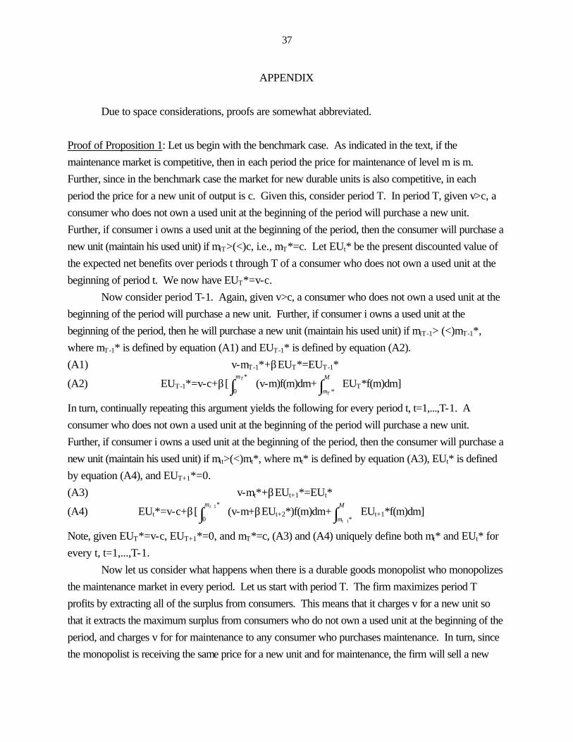
37

APPENDIX

Due to space considerations, proofs are somewhat abbreviated. Proof of Proposition 1: Let us begin with the benchmark case. As indicated in the text, if the maintenance market is competitive, then in each period the price for maintenance of level m is m. Further, since in the benchmark case the market for new durable units is also competitive, in each period the price for a new unit of output is c. Given this, consider period T. In period T, given v>c, a consumer who does not own a used unit at the beginning of the period will purchase a new unit. Further, if consumer i owns a used unit at the beginning of the period, then the consumer will purchase a new unit (maintain his used unit) if miT>(<)c, i.e., mT*=c. Let EUt* be the present discounted value of the expected net benefits over periods t through T of a consumer who does not own a used unit at the beginning of period t. We now have EUT*=v-c. Now consider period T-1. Again, given v>c, a consumer who does not own a used unit at the beginning of the period will purchase a new unit. Further, if consumer i owns a used unit at the beginning of the period, then he will purchase a new unit (maintain his used unit) if miT-1> (<)mT-1*, where mT-1* is defined by equation (A1) and EUT-1* is defined by equation (A2). (A1) v-mT-1*+βEUT*=EUT-1*

(A2) EUT-1*=v-c+β[ ∫*

0

Tm(v-m)f(m)dm+ ∫

M

mT *EUT*f(m)dm]

In turn, continually repeating this argument yields the following for every period t, t=1,...,T-1. A consumer who does not own a used unit at the beginning of the period will purchase a new unit. Further, if consumer i owns a used unit at the beginning of the period, then the consumer will purchase a new unit (maintain his used unit) if mit>(<)mt*, where mt* is defined by equation (A3), EUt* is defined by equation (A4), and EUT+1*=0. (A3) v-mt*+βEUt+1*=EUt*

(A4) EUt*=v-c+β[ ∫+ *

0

1tm(v-m+βEUt+2*)f(m)dm+ ∫

+

M

mt *1

EUt+1*f(m)dm]

Note, given EUT*=v-c, EUT+1*=0, and mT*=c, (A3) and (A4) uniquely define both mt* and EUt* for every t, t=1,...,T-1. Now let us consider what happens when there is a durable goods monopolist who monopolizes the maintenance market in every period. Let us start with period T. The firm maximizes period T profits by extracting all of the surplus from consumers. This means that it charges v for a new unit so that it extracts the maximum surplus from consumers who do not own a used unit at the beginning of the period, and charges v for for maintenance to any consumer who purchases maintenance. In turn, since the monopolist is receiving the same price for a new unit and for maintenance, the firm will sell a new

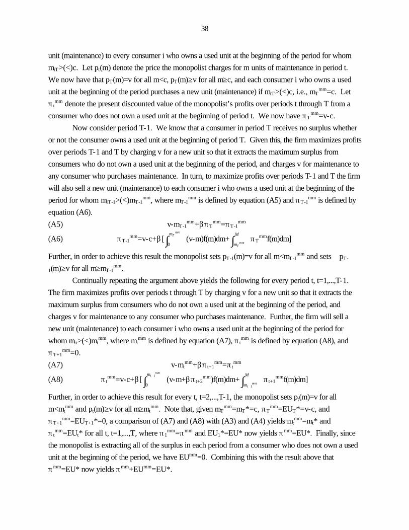
38

unit (maintenance) to every consumer i who owns a used unit at the beginning of the period for whom miT>(<)c. Let pt(m) denote the price the monopolist charges for m units of maintenance in period t. We now have that pT(m)=v for all m<c, pT(m)≥v for all m≥c, and each consumer i who owns a used unit at the beginning of the period purchases a new unit (maintenance) if miT>(<)c, i.e., mT

mm=c. Let π t

mm denote the present discounted value of the monopolist’s profits over periods t through T from a consumer who does not own a used unit at the beginning of period t. We now have πT

mm=v-c. Now consider period T-1. We know that a consumer in period T receives no surplus whether or not the consumer owns a used unit at the beginning of period T. Given this, the firm maximizes profits over periods T-1 and T by charging v for a new unit so that it extracts the maximum surplus from consumers who do not own a used unit at the beginning of the period, and charges v for maintenance to any consumer who purchases maintenance. In turn, to maximize profits over periods T-1 and T the firm will also sell a new unit (maintenance) to each consumer i who owns a used unit at the beginning of the period for whom miT-1>(<)mT-1

mm, where mT-1mm is defined by equation (A5) and πT-1

mm is defined by equation (A6). (A5) v-mT-1

mm+βπTmm=πT-1

mm

(A6) πT-1mm=v-c+β[ ∫

mmTm

0(v-m)f(m)dm+ ∫

M

m mmT

πTmmf(m)dm]

Further, in order to achieve this result the monopolist sets pT-1(m)=v for all m<mT-1mm and sets pT-

1(m)≥v for all m≥mT-1mm.

Continually repeating the argument above yields the following for every period t, t=1,...,T-1. The firm maximizes profits over periods t through T by charging v for a new unit so that it extracts the maximum surplus from consumers who do not own a used unit at the beginning of the period, and charges v for maintenance to any consumer who purchases maintenance. Further, the firm will sell a new unit (maintenance) to each consumer i who owns a used unit at the beginning of the period for whom mit>(<)mt

mm, where mtmm is defined by equation (A7), π t

mm is defined by equation (A8), and πT+1

mm=0. (A7) v-mt

mm+βπ t+1mm=π t

mm

(A8) π tmm=v-c+β[ ∫

+mm

tm 1

0(v-m+βπ t+2

mm)f(m)dm+ ∫+

M

m mmt 1

π t+1mmf(m)dm]

Further, in order to achieve this result for every t, t=2,...,T-1, the monopolist sets pt(m)=v for all m<mt

mm and pt(m)≥v for all m≥mtmm. Note that, given mT

mm=mT*=c, πTmm=EUT*=v-c, and

πT+1mm=EUT+1*=0, a comparison of (A7) and (A8) with (A3) and (A4) yields mt

mm=mt* and π t

mm=EUt* for all t, t=1,...,T, where π1mm=πmm and EU1*=EU* now yields πmm=EU*. Finally, since

the monopolist is extracting all of the surplus in each period from a consumer who does not own a used unit at the beginning of the period, we have EUmm=0. Combining this with the result above that πmm=EU* now yields πmm+EUmm=EU*.

39

Now let us consider what happens when there is a durable goods monopolist and the maintenance market is competitive in every period. Let us start with period T. To extract all of the surplus from a consumer who does not own a used unit at the beginning of the period, the firm charges v for a new unit. Given this, if the firm offers to repurchase a used unit at a price greater than or equal to v-c, then the firm earns zero or negative profits from the sale of new units to consumers who own used units at the beginning of the period. Hence, in order to maximize period T profits, the firm offers a repurchase price in period T that is strictly below v-c. Also, because the firm has constant returns to scale in the production of new units, the unique repurchase price that maximizes period T profits is independent of the number of consumers who own used units at the beginning of the period (see footnote 4). We now have that a consumer who does not own a used unit at the beginning of the period purchases a new unit at the price v. Further, if consumer i owns a used unit at the beginning of the period, then the consumer will purchase a new unit (maintain his used unit) if miT>(<)mT

mc, where because the price for a replacement unit is above c we have mT

mc>mTmm=mT*=c.

Let π tmc denote the present discounted value of the monopolist’s expected profits over periods t

through T from a consumer who does not own a used unit at the beginning of period t, and let π tmc′

denote the present discounted value of the monopolist’s expected profits over periods t through T from a consumer who does own a used unit at the beginning of period t (where π t

mc′ is not conditioned on the maintenance realization in period t). We have that πT

mc= v-c. Also, let EUtmc be the present

discounted value of the expected net benefits over periods t through T of a consumer who does not own a used unit at the beginning of period t, and let EUt

mc′ be the present discounted value of the expected net benefits over periods t through T of a consumer who does own a used unit at the beginning of period t (where EUt

mc′ is not conditioned on the maintenance realization in period t). We have that EUTmc=0.

Now consider period T-1. To extract all of the surplus from consumers who do not own used units at the beginning of the period, the firm charges v+βEUT

mc′ for a new unit. This means EUT-1mc=0.

We also know that since consumers do not make efficient maintenance decisions in period T and since the firm is able to extract all of the surplus when it monopolizes the maintenance market in every period, it must be the case that πT-1

mc<πT-1mm. Now consider consumers who own used units at the beginning

of period T-1. Since the firm earns βπTmc from each such consumer who does not purchase a new unit

in period T-1 and earns in period T an expected amount of πTmc′ from a consumer who purchases a

new unit in period T-1, to maximize profits over periods T-1 through T the firm will offer a repurchase price such that the price for a replacement unit is strictly greater than c+βπT

mc-βπTmc′. Given this and

EUTmc=0, we have that mT-1

mc must satisfy equation (A9). (A9) v-mT-1

mc<v-c-βπTmc+βπT

mc′+βEUTmc′

(A9) can be rewritten as (A10). (A10) v-mT-1

mc+βπTmc<v-c+β(πT

mc′+EUTmc′)

40

Since mTmc>mT

mm=mT*, we know that v-c+β(πTmc′+EUT

mc′)<πT-1mm. We also know that

πTmc=πT

mm=v-c. Hence, a comparison of (A5) and (A10) yields mT-1mc>mT-1

mm=mT-1*. We now have that a consumer who does not own a used unit at the beginning of the period purchases a new unit at the price v+βEUT

mc′. Further, if consumer i owns a used unit at the beginning of the period, then the consumer will purchase a new unit (maintain his used unit) if miT-1>(<)mT-1

mc, where mT-1mc>mT-1

mm= mT-1*. Continually repeating the first steps of the above argument yields the following for every period t, t=1,...,T-1. To extract all of the surplus from consumers who do not own used units at the beginning of the period, the firm charges v+βEUt+1

mc′ for a new unit. This means EUtmc=0. We also know that

since consumers do not make efficient maintenance decisions in period T and since the firm is able to extract all of the surplus when it monopolizes the maintenance market in every period, it must be the case that π t

mc<π tmm. We now have that a consumer who does not own a used unit at the beginning of

the period purchases a new unit at the price v+βEUt+1mc′. Further, there exists a value mt

mc such that a consumer who owns a used unit at the beginning of the period purchases a new unit (maintains his used unit) if mit>(<)mt

mc, but we have been unable to derive a result comparing mtmc and mt* except for t=T-

1 and t=T. Finally, since πmc=π1mc and EUmc=EU1

mc, we now have that πmc<πmm, EUmc=EUmm=0, and πmc+EUmc<πmm+EUmm=EU*. The final step is to consider the monopolist’s choice whether or not to monopolize the maintenance market when it has that choice in each period. Consider period T. Since the firm extracts all of the surplus by monopolizing the maintenance market and does not extract all of the surplus if it does not, independent of what has happened in the past, the firm maximizes its profits in period T by monopolizing the maintenance market. Now consider period T-1. Given the firm will monopolize the maintenance market in period T, we have that the firm extracts all of the surplus over periods T-1 and T by monopolizing the maintenance market in period T-1 and does not extract all of the surplus if it does not. Hence, the firm monopolizes the maintenance market in period T-1. Finally, continually repeating the above argument yields that the monopolist chooses to monopolize the maintenance market in each period t, 2≤t≤T. Proof of Proposition 2: As indicated in the text, the benchmark case here is the same as in Proposition 1. Given this, let us consider what happens when each durable goods producer monopolizes the maintenance market in each period. Our focus will be on producer j where producer j sells a strictly positive number of new units in the first period. Let π jt

cm denote the present discounted value of the expected profits that firm j derives over periods t through T from selling to a consumer who consumed a unit of the firm’s product in period t-1 but who does not own a used unit at the beginning of period t. Also, let Pt

Em be the price that a new entrant in period t is willing to sell a new unit for in period t (see

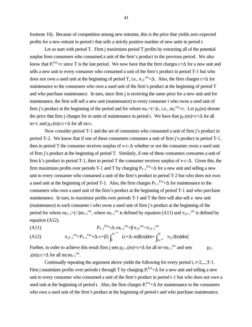
41

footnote 16). Because of competition among new entrants, this is the price that yields zero expected profits for a new entrant in period t that sells a strictly positive number of new units in period t. Let us start with period T. Firm j maximizes period T profits by extracting all of the potential surplus from consumers who consumed a unit of the firm’s product in the previous period. We also know that Pt

Em=c since T is the last period. We now have that the firm charges c+∆ for a new unit and sells a new unit to every consumer who consumed a unit of the firm’s product in period T-1 but who does not own a used unit at the beginning of period T, i.e., π jT

cm=∆. Also, the firm charges c+∆ for maintenance to the consumers who own a used unit of the firm’s product at the beginning of period T and who purchase maintenance. In turn, since firm j is receiving the same price for a new unit and for maintenance, the firm will sell a new unit (maintenance) to every consumer i who owns a used unit of firm j’s product at the beginning of the period and for whom miT>(<)c, i.e., mT

cm=c. Let pjt(m) denote the price that firm j charges for m units of maintenance in period t. We have that pjT(m)=c+∆ for all m<c and pjT(m)≥c+∆ for all m≥c. Now consider period T-1 and the set of consumers who consumed a unit of firm j’s product in period T-2. We know that if one of these consumers consumes a unit of firm j’s product in period T-1, then in period T the consumer receives surplus of v-c-∆ whether or not the consumer owns a used unit of firm j’s product at the beginning of period T. Similarly, if one of these consumers consumes a unit of firm k’s product in period T-1, then in period T the consumer receives surplus of v-c-∆. Given this, the firm maximizes profits over periods T-1 and T by charging PT-1

Em+∆ for a new unit and selling a new unit to every consumer who consumed a unit of the firm’s product in period T-2 but who does not own a used unit at the beginning of period T-1. Also, the firm charges PT-1

Em+∆ for maintenance to the consumers who own a used unit of the firm’s product at the beginning of period T-1 and who purchase maintenance. In turn, to maximize profits over periods T-1 and T the firm will also sell a new unit (maintenance) to each consumer i who owns a used unit of firm j’s product at the beginning of the period for whom miT-1>(<)mT-1

cm, where mT-1cm is defined by equation (A11) and π jT-1

cm is defined by equation (A12). (A11) PT-1

Em+∆-mT-1cm+βπ jT

cm=π jT-1cm

(A12) π jT-1cm=PT-1

Em+∆-c+β[ ∫cm

Tm

0(c+∆-m)f(m)dm+ ∫

M

m cmT

π jTf(m)dm]

Further, in order to achieve this result firm j sets pjT-1(m)=c+∆ for all m<mT-1cm and sets pjT-

1(m)≥c+∆ for all m≥mT-1cm.

Continually repeating the argument above yields the following for every period t, t=2,...,T-1. Firm j maximizes profits over periods t through T by charging Pt

Em+∆ for a new unit and selling a new unit to every consumer who consumed a unit of the firm’s product in period t-1 but who does not own a used unit at the beginning of period t. Also, the firm charges Pt

Em+∆ for maintenance to the consumers who own a used unit of the firm’s product at the beginning of period t and who purchase maintenance.

42

In turn, to maximize profits over periods t through T the firm will also sell a new unit (maintenance) to each consumer i who owns a used unit of firm j’s product at the beginning of the period for whom mit>(<)mt

cm, where mtcm is defined by equation (A13), π jt

cm is defined by equation (A14), and π jT+1

cm=0. (A13) Pt

Em+∆-mtcm+βπ jt+1

cm=π jtcm

(A14) π jtcm=Pt

Em+∆-c+β[ ∫+

cmtm 1

0(Pt+1

Em+∆-m+βπ jt+2cm)f(m)dm+ ∫

+

M

m cmt 1

π jt+1cmf(m)dm]

Further, in order to achieve this result for every t, t=2,...,T-1, firm j sets pjt(m)=PtEm+∆ for all m<mt

cm and pjt(m)≥Pt

Em+∆ for all m≥mtcm.

We can now compare mtcm with mt*. From above we know mT

cm=mT*=c and πTcm=∆, while

from the proof of Proposition 1 we know EUT*=v-c. Now consider period T-1. Given mT*=c, EUT*=v-c, and EUT+1*=0, (A3) reduces to (A15).

(A15) v-mT-1*+β(v-c)=v-c+β[ ∫c

0(v-m)f(m)dm+ ∫

M

c(v-c)f(m)dm]

(A15) yields (A16).

(A16) mT-1*=c-β[ ∫c

0(c-m)f(m)dm]

Given mTcm=c, PT

Em=c, πTcm=∆, and πT+1

cm=0, (A13) reduces to (A17).

(A17) PT-1Em+∆-mT-1

cm+β∆=PT-1Em+∆-c+β[ ∫

c

0(c+∆-m)f(m)dm+ ∫

M

c∆f(m)dm]

(A17) yields (18).

(A18) mT-1cm=c-β[ ∫

c

0(c-m)f(m)dm]

(A16) and (A18) yield mT-1cm=mT-1*. In turn, repeating these steps for earlier periods yields mt

cm=mt* for all t, t=2,...,T. Finally, competition in the first period yields that over the T periods every durable goods producer earns zero expected profits. Combining this with mt

cm=mt* for all t, 2≤t≤T and that each consumer never switches producers during the T periods yields that EUcm=EU*. Now let us consider what happens when the maintenance market is competitive each period for every durable goods producer’s product. Our focus is again on durable goods producer j where producer j sells a strictly positive number of new units in the first period. Let π jt

cc denote the present discounted value of the expected profits that firm j derives over periods t through T from selling to a consumer who consumed a unit of the firm’s product in period t-1 but who does not own a used unit at the beginning of period t, while π jt

cc′ denotes the present discounted value of the expected profits that firm j derives over periods t through T from a consumer who consumed a unit of the firm’s product in period t-1 and who does own a used unit at the beginning of period t (where π jt

cc′ is not conditioned on the maintenance realization in period t). Let EUt

cc be the present discounted value of the expected net benefits over periods t through T of a consumer who consumed a unit of the firm’s product in period t-1 and who does not own a used unit at the beginning of period t, while EUt

cc′ is the present discounted

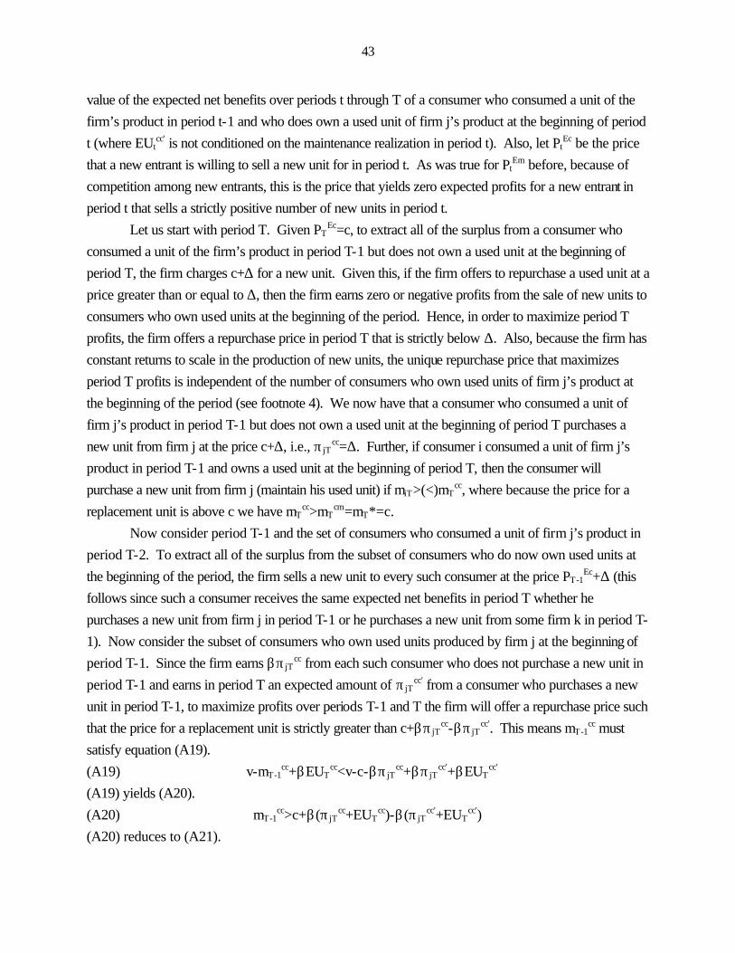
43

value of the expected net benefits over periods t through T of a consumer who consumed a unit of the firm’s product in period t-1 and who does own a used unit of firm j’s product at the beginning of period t (where EUt

cc′ is not conditioned on the maintenance realization in period t). Also, let PtEc be the price

that a new entrant is willing to sell a new unit for in period t. As was true for PtEm before, because of

competition among new entrants, this is the price that yields zero expected profits for a new entrant in period t that sells a strictly positive number of new units in period t. Let us start with period T. Given PT

Ec=c, to extract all of the surplus from a consumer who consumed a unit of the firm’s product in period T-1 but does not own a used unit at the beginning of period T, the firm charges c+∆ for a new unit. Given this, if the firm offers to repurchase a used unit at a price greater than or equal to ∆, then the firm earns zero or negative profits from the sale of new units to consumers who own used units at the beginning of the period. Hence, in order to maximize period T profits, the firm offers a repurchase price in period T that is strictly below ∆. Also, because the firm has constant returns to scale in the production of new units, the unique repurchase price that maximizes period T profits is independent of the number of consumers who own used units of firm j’s product at the beginning of the period (see footnote 4). We now have that a consumer who consumed a unit of firm j’s product in period T-1 but does not own a used unit at the beginning of period T purchases a new unit from firm j at the price c+∆, i.e., π jT

cc=∆. Further, if consumer i consumed a unit of firm j’s product in period T-1 and owns a used unit at the beginning of period T, then the consumer will purchase a new unit from firm j (maintain his used unit) if miT>(<)mT

cc, where because the price for a replacement unit is above c we have mT

cc>mTcm=mT*=c.

Now consider period T-1 and the set of consumers who consumed a unit of firm j’s product in period T-2. To extract all of the surplus from the subset of consumers who do now own used units at the beginning of the period, the firm sells a new unit to every such consumer at the price PT-1

Ec+∆ (this follows since such a consumer receives the same expected net benefits in period T whether he purchases a new unit from firm j in period T-1 or he purchases a new unit from some firm k in period T-1). Now consider the subset of consumers who own used units produced by firm j at the beginning of period T-1. Since the firm earns βπ jT

cc from each such consumer who does not purchase a new unit in period T-1 and earns in period T an expected amount of π jT

cc′ from a consumer who purchases a new unit in period T-1, to maximize profits over periods T-1 and T the firm will offer a repurchase price such that the price for a replacement unit is strictly greater than c+βπ jT

cc-βπ jTcc′. This means mT-1

cc must satisfy equation (A19). (A19) v-mT-1

cc+βEUTcc<v-c-βπ jT

cc+βπ jTcc′+βEUT

cc′ (A19) yields (A20). (A20) mT-1

cc>c+β(π jTcc+EUT

cc)-β(π jTcc′+EUT

cc′) (A20) reduces to (A21).

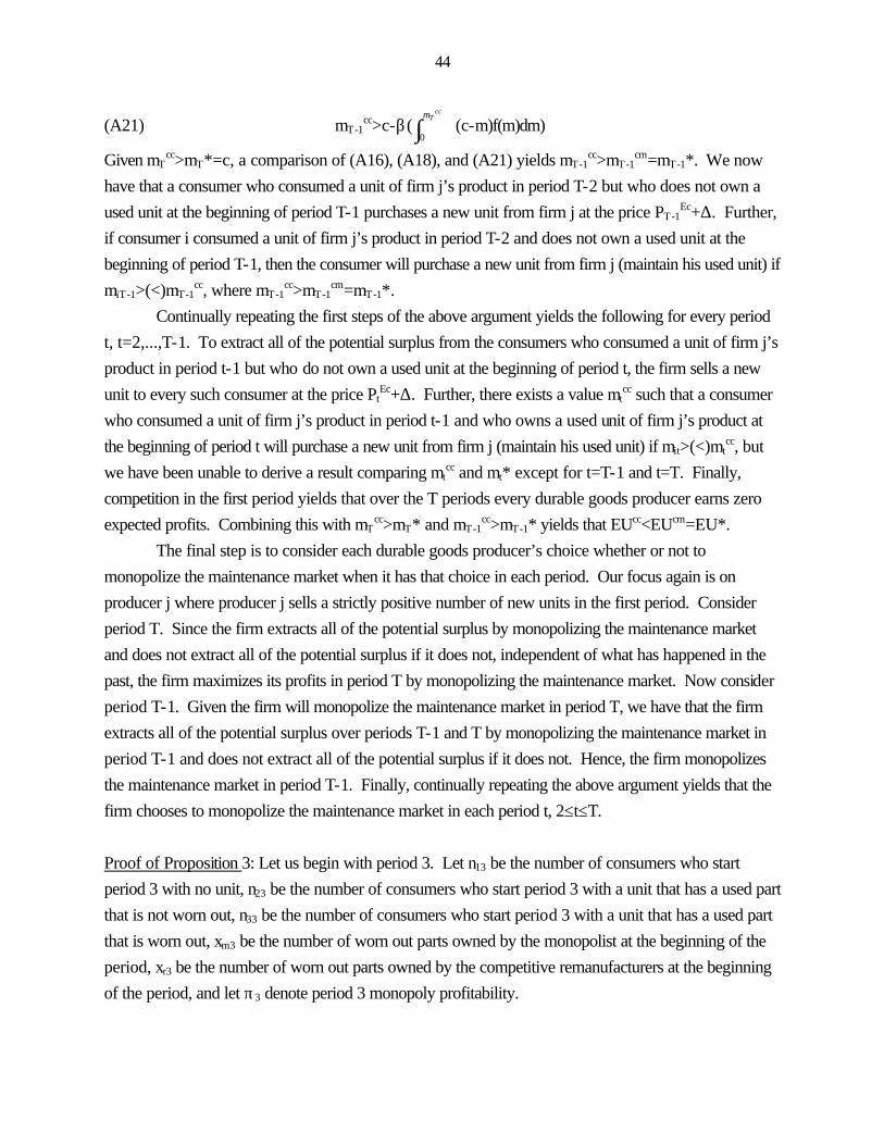
44

(A21) mT-1cc>c-β( ∫

ccTm

0(c-m)f(m)dm)

Given mTcc>mT*=c, a comparison of (A16), (A18), and (A21) yields mT-1

cc>mT-1cm=mT-1*. We now

have that a consumer who consumed a unit of firm j’s product in period T-2 but who does not own a used unit at the beginning of period T-1 purchases a new unit from firm j at the price PT-1

Ec+∆. Further, if consumer i consumed a unit of firm j’s product in period T-2 and does not own a used unit at the beginning of period T-1, then the consumer will purchase a new unit from firm j (maintain his used unit) if miT-1>(<)mT-1

cc, where mT-1cc>mT-1

cm=mT-1*. Continually repeating the first steps of the above argument yields the following for every period t, t=2,...,T-1. To extract all of the potential surplus from the consumers who consumed a unit of firm j’s product in period t-1 but who do not own a used unit at the beginning of period t, the firm sells a new unit to every such consumer at the price Pt

Ec+∆. Further, there exists a value mtcc such that a consumer

who consumed a unit of firm j’s product in period t-1 and who owns a used unit of firm j’s product at the beginning of period t will purchase a new unit from firm j (maintain his used unit) if mit>(<)mt

cc, but we have been unable to derive a result comparing mt

cc and mt* except for t=T-1 and t=T. Finally, competition in the first period yields that over the T periods every durable goods producer earns zero expected profits. Combining this with mT

cc>mT* and mT-1cc>mT-1* yields that EUcc<EUcm=EU*.

The final step is to consider each durable goods producer’s choice whether or not to monopolize the maintenance market when it has that choice in each period. Our focus again is on producer j where producer j sells a strictly positive number of new units in the first period. Consider period T. Since the firm extracts all of the potential surplus by monopolizing the maintenance market and does not extract all of the potential surplus if it does not, independent of what has happened in the past, the firm maximizes its profits in period T by monopolizing the maintenance market. Now consider period T-1. Given the firm will monopolize the maintenance market in period T, we have that the firm extracts all of the potential surplus over periods T-1 and T by monopolizing the maintenance market in period T-1 and does not extract all of the potential surplus if it does not. Hence, the firm monopolizes the maintenance market in period T-1. Finally, continually repeating the above argument yields that the firm chooses to monopolize the maintenance market in each period t, 2≤t≤T. Proof of Proposition 3: Let us begin with period 3. Let n13 be the number of consumers who start period 3 with no unit, n23 be the number of consumers who start period 3 with a unit that has a used part that is not worn out, n33 be the number of consumers who start period 3 with a unit that has a used part that is worn out, xm3 be the number of worn out parts owned by the monopolist at the beginning of the period, xr3 be the number of worn out parts owned by the competitive remanufacturers at the beginning of the period, and let π3 denote period 3 monopoly profitability.

45

Because p2>p1, it must be the case that xm3+xr3<n33 (this follows since every used unit in the second period will also be a used unit in the third period, and some used units in the third period have a probability p2 of having a worn out part while every used unit in the second period has a probability p1 of having a worn out part). To maximize π3 the monopolist will do the following. First, if n13>0 the monopolist will set a price for a new unit equal to v to extract all of the surplus from each consumer who does not own a used unit at the beginning of the period, and each such consumer purchases a new unit from the monopolist. Second, if n33>0 the monopolist will set a price for a new part equal to M+z in order to extract all of the surplus from consumers who purchase new parts from the monopolist and, because new and remanufactured parts are perfect substitutes, remanufactured parts also sell for M+z. The result is that every consumer with a worn out part purchases either a new part or a remanufactured part and scraps the worn out part. We now have that third period monopoly profitability is given by π3=n13(v-c)+xm3(M+z -cr′)+(n33-xm3-xr3)(M+z-cp). Now consider period 2. Let n12 be the number of consumers who start period 2 with no unit, n22 be the number of consumers who start period 2 with a unit that has a used part that is not worn out, n32 be the number of consumers who start period 2 with a unit that has a used part that is worn out, and let π2 be the present discounted value of the firm’s flow of profits over periods 2 and 3. There are two cases. Suppose n12=1. From before we know that a consumer who does not purchase a new unit in the second period has expected consumer surplus over the second and third periods equal to zero. Given this and the equilibrium behavior in the third period described above, a consumer will be willing to pay up to (1+β)v-βp1M for a new unit in the second period. Given this and the equilibrium behavior in the third period described above, the result is that the monopolist charges (1+β)v-βp1M for a new unit in the second period, every consumer purchases a new unit in the second period, and π2=(1+β)v-c+βp1(z-cp). Now suppose n12<1. As before, the monopolist will set the price for a new unit in the second period equal to (1+β)v-βp1M and every consumer who does not own a new unit at the beginning of the period will purchase a new unit from the monopolist. Further, given our analysis of period 3, competition among competitive remanufacturers yields that these firms will offer β(M+z-cr) for a worn out part in the second period. Given this and assuming that the monopolist sells a new part to every consumer who owns a worn out part, in the second period the monopolist has three relevant options in terms of the price it sets for a new part and the core charge. These three options are as follows. First, the monopolist could set the core charge sufficiently low that it does not repurchase any worn out parts and set P2

p=M+β(M+z-cr). This yields π2=n12[(1+β)v-c+βp1(z-cp)]+n32[M-cp+β(M+z-cr)]+βA[M+z-cp], where A=p2n22+p1n32+p1n12-n32 (note that since n12+n22+n32=1, p2>p1, and n32≤p1, we know A>0). Second, the monopolist could purchase some but not all of the worn out parts. This means P′=β(M+z-cr) and P2

p=M+β(M+z-cr) (note that any lower core charge means the monopolist purchases no worn out parts while any higher core charge means that it purchases all of the

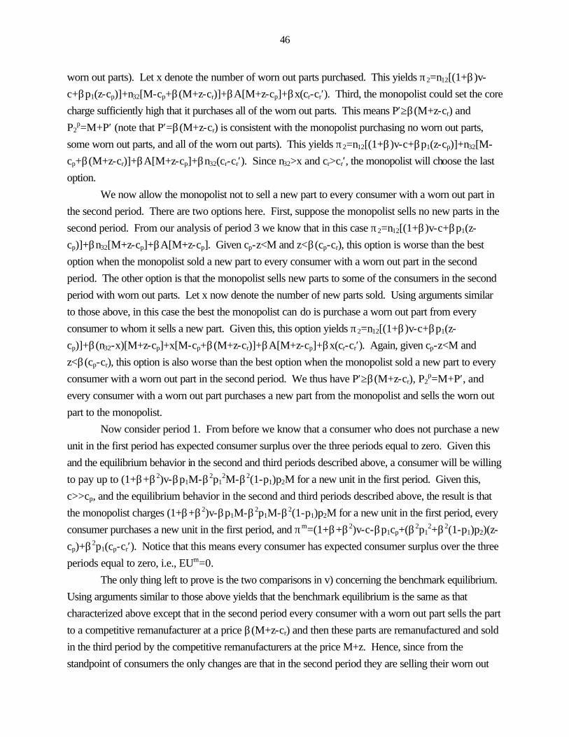
46

worn out parts). Let x denote the number of worn out parts purchased. This yields π2=n12[(1+β)v-c+βp1(z-cp)]+n32[M-cp+β(M+z-cr)]+βA[M+z-cp]+βx(cr-cr′). Third, the monopolist could set the core charge sufficiently high that it purchases all of the worn out parts. This means P′≥β(M+z-cr) and P2

p=M+P′ (note that P′=β(M+z-cr) is consistent with the monopolist purchasing no worn out parts, some worn out parts, and all of the worn out parts). This yields π2=n12[(1+β)v-c+βp1(z-cp)]+n32[M-cp+β(M+z-cr)]+βA[M+z-cp]+βn32(cr-cr′). Since n32>x and cr>cr′, the monopolist will choose the last option. We now allow the monopolist not to sell a new part to every consumer with a worn out part in the second period. There are two options here. First, suppose the monopolist sells no new parts in the second period. From our analysis of period 3 we know that in this case π2=n12[(1+β)v-c+βp1(z-cp)]+βn32[M+z-cp]+βA[M+z-cp]. Given cp-z<M and z<β(cp-cr), this option is worse than the best option when the monopolist sold a new part to every consumer with a worn out part in the second period. The other option is that the monopolist sells new parts to some of the consumers in the second period with worn out parts. Let x now denote the number of new parts sold. Using arguments similar to those above, in this case the best the monopolist can do is purchase a worn out part from every consumer to whom it sells a new part. Given this, this option yields π2=n12[(1+β)v-c+βp1(z-cp)]+β(n32-x)[M+z-cp]+x[M-cp+β(M+z-cr)]+βA[M+z-cp]+βx(cr-cr′). Again, given cp-z<M and z<β(cp-cr), this option is also worse than the best option when the monopolist sold a new part to every consumer with a worn out part in the second period. We thus have P′≥β(M+z-cr), P2

p=M+P′, and every consumer with a worn out part purchases a new part from the monopolist and sells the worn out part to the monopolist. Now consider period 1. From before we know that a consumer who does not purchase a new unit in the first period has expected consumer surplus over the three periods equal to zero. Given this and the equilibrium behavior in the second and third periods described above, a consumer will be willing to pay up to (1+β+β2)v-βp1M-β2p1

2M-β2(1-p1)p2M for a new unit in the first period. Given this, c>>cp, and the equilibrium behavior in the second and third periods described above, the result is that the monopolist charges (1+β+β2)v-βp1M-β2p1M-β2(1-p1)p2M for a new unit in the first period, every consumer purchases a new unit in the first period, and πm=(1+β+β2)v-c-βp1cp+(β2p1

2+β2(1-p1)p2)(z-cp)+β2p1(cp-cr′). Notice that this means every consumer has expected consumer surplus over the three periods equal to zero, i.e., EUm=0. The only thing left to prove is the two comparisons in v) concerning the benchmark equilibrium. Using arguments similar to those above yields that the benchmark equilibrium is the same as that characterized above except that in the second period every consumer with a worn out part sells the part to a competitive remanufacturer at a price β(M+z-cr) and then these parts are remanufactured and sold in the third period by the competitive remanufacturers at the price M+z. Hence, since from the standpoint of consumers the only changes are that in the second period they are selling their worn out

47

parts to different firms (but at the same price) and that in the third period they are buying the remanufactured parts from different firms (but at the same price), there is no effect on consumer welfare, i.e., EUm=EU*=0. Further, since the monopolist is no longer participating in the remanufacturing market, monopoly profitability is now given by π*=(1+β+β2)v-c-βp1cp-(β2p1

2+β2(1-p1)p2)(z-cp)+β2p1(cp-cr). Since cr>cr′, we have πm>π*.

REFERENCES

Borenstein, S., J. Mackie-Mason, and J. Netz, “Antitrust Policy in Aftermarkets,” Antitrust Law

Journal, 1995, 63, 455-482.

Bulow, J., “Durable Goods Monopolists,” Journal of Political Economy, 1982, 90, 314-332.

Carlton, D., “Refusal to Deal – Must a Firm Help its Rival,” mimeo, University of Chicago,

April 2000 (Forthcoming Antitrust Law Journal).

Chen, Z., and T. Ross, “Refusals to Deal, Price Discrimination, and Independent Service

Organizations,” Journal of Economics and Management Strategy, 1994, 2, 593-614.

Chen, Z., and T. Ross, “Orders to Supply as Substitutes for Commitments to Aftermarkets,”

Canadian Journal of Economics, 1998, 31, 1204-1224.

Chen, Z., T. Ross, and W. Stanbury, “Refusals to Deal and Aftermarkets,” Review of Industrial

Organization, 1998, 13, 131-151.

48

Coase, R., “Durability and Monopoly,” Journal of Law and Economics, 1972, 15, 143-149.

Farrell, J., and C. Shapiro, “Dynamic Competition with Switching Costs,” Rand Journal of

Economics, 1988, 19, 123-137.

Farrell, J., and C. Shapiro, “Optimal Contracts with Lock-In,” American Economic Review,

1989, 79, 51-68.

Fudenberg, D., and J. Tirole, “Upgrades, Tradeins, and Buybacks,” Rand Journal of Economics,

1998, 29, 235-258.

Hendel, I., and A. Lizzeri, “Interfering with Secondary Markets,” Rand Journal of Economics,

1999, 30, 1-21.

Klein, B., “Market Power in Antitrust: Economic Analysis After Kodak,” Supreme Court

Economic Review, 1993, 3, 43-92.

Klemperer, P., “Markets with Consumer Switching Costs,” Quarterly Journal of Economics,

1987, 102, 375-394.

Klemperer, P., “Price Wars Caused by Switching Costs,” Review of Economic Studies, 1989,

56, 405-420.

Klemperer, P., “Competition when Consumers have Switching Costs: An Overview with

Applications to Industrial Organization, Macroeconomics, and International Trade,”

Review of Economic Studies, 1995, 62, 515-539.

Mallela, P., and B. Nahata, “Theory of Vertical Control with Variable Proportions,” Journal of

Political Economy, 1980, 88, 1009-1025.

Morita, H., and M. Waldman, “Competition, Monopoly Maintenance, and Consumer Switching

Costs,” mimeo, Cornell University, February 2000.

Plaintiff’s Memorandum in Eastman Kodak Co. v. Image Technical Services, 1992.

Rust, J., “When is it Optimal to Kill Off the Market for Used Durable Goods?,” Econometrica,

1986, 54, 65-86.

Salop, S., “The Kodak Case, the First Principles Approach, and Antitrust at the Millenium,”

Mimeo, Georgetown University, 1999.

49

Schmalensee, R., “Market Structure, Durability, and Maintenance Effort,” Review of Economic

Studies, 1974, 41, 277-287.

Shapiro, C., “Aftermarkets and Consumer Welfare: Making Sense of Kodak,” Antitrust Law

Journal, 1995, 63, 148-157.

Stokey, N., “Rational Expectations and Durable Goods Pricing,” Bell Journal of Economics,

1981, 12, 112-128.

Su, T., “Durability of Consumption Goods Reconsidered,” American Economic Review, 1975,

65, 148-157.

Waldman, M., “Durable Goods Pricing When Quality Matters,” Journal of Business, 1996, 69,

489-510.

Waldman, M., “Eliminating the Market for Secondhand Goods: An Alternative Explanation for

Leasing,” Journal of Law and Economics, 1997, 40, 61-92.

Williamson, O., Markets and Hierarchies: Analysis and Antitrust Implications, New York: The

Free Press, 1975.

Williamson, O., Economic Institutions of Capitalism, New York: The Free Press, 1985.