Competition, markups, and gains from trade: A quantitative ...

Journal of International Economics 122 (2020) 103266

Contents lists available at ScienceDirect

Journal of International Economics

j ourna l homepage: www.e lsev ie r .com/ locate / j i e

Full Length Articles

Competition, markups, and gains from trade: A quantitative analysisof China between 1995 and 2004

Wen-Tai Hsu a,⁎, Yi Lu b, Guiying Laura Wu c

a School of Economics, Singapore Management University. 90 Stamford Road, 178903, Singaporeb School of Economics and Management, Tsinghua University, Beijing 100084, Chinac Division of Economics, School of Humanities and Social Sciences, Nanyang Technological University, 14 Nanyang Drive, 637332, Singapore

⁎ Corresponding author.E-mail addresses: [email protected] (W.-T. Hsu)

(Y. Lu), [email protected] (G.L. Wu).1 The idea of allocative efficiency dates back to Robinso

Lancaster (1956-57). Note that allocative efficiency is deteresources are allocated across firms with different markuemployment and the dispersion of markups matter.Arkolakis et al. (2019) and also in the formulation of the c

https://doi.org/10.1016/j.jinteco.2019.1032660022-1996/© 2019 Elsevier B.V. All rights reserved.

a b s t r a c t
a r t i c l e i n f o
Article history:Received 2 August 2017Received in revised form 27 September 2019Accepted 12 October 2019Available online 4 November 2019

This paper provides a quantitative analysis of gains from trade in a model with head-to-head competition usingChinese firm-level data from Economic Censuses in 1995 and 2004. We find a significant reduction in trade costduring this period, and total gains from such improved openness during this period is 7.1%. The gains aredecomposed into a Ricardian component and two pro-competitive ones. The pro-competitive effects accountfor 20% of the total gains. Moreover, the total gains from trade are 13 − 31% larger than what would resultfrom the formula provided by ACR (Arkolakis et al., 2012), which nests a class of important trade models, butwithout pro-competitive effects. We find that head-to-head competition is the key reason behind the largergains, as trade flows do not reflect all of the effects via markups in an event of trade liberalization.

© 2019 Elsevier B.V. All rights reserved.

Key words:Gains from tradeMarkupsPro-competitive effectsACR formulaHead-to-head competitionChinese economy

1. Introduction

It has been well understood that competition may affect gains fromtrade via changes in the distribution of markups. For example, whenmarkups are the same across all goods, first-best allocative efficiencyis attained because the condition that the price ratio equals themarginalcost ratio, for any pair of goods, holds. In other words, in an economywith variable markups, trade liberalization may improve allocative effi-ciency if the dispersion of markups is reduced.1 Moreover, the relativemarkup effect alsomatters because welfare improves with trade liberal-ization when consumers benefit from lower markups of the goods theyconsume andwhen producers gain from highermarkups (hence higherprofits) in foreignmarkets. The effects of trade liberalization via changesin both the mean and dispersion of markups are generally termed pro-competitive effects of trade.

, [email protected]

n (1934, Ch. 27) and Lipsey andrmined by how the productionps. Thus, both relative revenue/This point is made clear byurrent paper.

A natural question is then whether competition and markups arequantitatively important in gains from trade. To address this, this paperconducts quantitative analyses of the gains from trade using a modelthat features head-to-head competition to investigate the role of pro-competitive effects. We use Chinese firm-level data in Economic Cen-suses in 1995 and 2004 to quantify our model. China in between thesetwo years is an important case, as this was a period when China drasti-cally improved openness – not onlywas transport infrastructure rapidlyexpanded, but joining the World Trade Organization (WTO) in 2001also drastically reduced trade barriers.2 Recently, Brandt et al. (2017)and Lu and Yu (2015) have both estimated firm-level markups usingChinese manufacturing data and the approach by De Loecker andWarzynski (2012; henceforth DLW). Lu and Yu (2015) show that thelarger the tariff reduction due to the WTO entry in one industry, thegreater the reduction in the dispersion of markups in that industry.Brandt et al. present similar results on levels of markups. These empiri-cal results suggest that pro-competitive effects might be present in thecase of China, but a formal quantitative welfare analysis is warranted.

2 Between 1995 and 2004, the import share increased from 0.13 to 0.22, whereas theexport share increased from 0.15 to 0.25. The proportion of exporters amongmanufactur-ing firms also increased from 4.4% to 10.5%.

http://crossmark.crossref.org/dialog/?doi=10.1016/j.jinteco.2019.103266&domain=pdf

https://doi.org/10.1016/j.jinteco.2019.103266

mailto:[email protected]



Journal logo

https://doi.org/10.1016/j.jinteco.2019.103266

Unlabelled image

http://www.sciencedirect.com/science/journal/00221996

www.elsevier.com/locate/jie

Fig. 1. Markup distributions (1995 versus 2004).

5 For the intuition behind the low trade elasticities in our estimatedmodels, see Section4.2.

6

2 W.-T. Hsu et al. / Journal of International Economics 122 (2020) 103266

The two focuses of ourwelfare analyses are howhead-to-head compe-titionmatters for the total gains from trade and the decomposition of thesetotal gains into a standard Ricardian component and pro-competitive ef-fects. To appreciate what we do, it is important to review recent relatedstudies. First, Arkolakis et al. (2012; henceforth ACR) show that for a

class of influential trade models, welfare gains from trade (W ≡W 0=W)

can be simply calculated by ðv0=vÞ1=ϵ ¼ v1=ϵ, where v is domestic expendi-ture share, and ϵ b 0 is the trade elasticity. As both v and ϵ depend on tradeflows, trade flows provide key information regarding gains from trade.However, this class of models features no pro-competitive effects. To in-vestigate pro-competitive effects, Edmond et al. (2015; henceforth EMX)use a model of distinct-product Cournot competition a lá Atkeson andBurstein (2008) and find that pro-competitive effects account for 11− 38% of total gains from trade. Moreover, even though EMX’s model de-viates from the ACR class and sizable pro-competitive effects are found, itturns out their total gains from trade is well captured by the local versionof the ACR formula. Similar results are also found by Feenstra andWeinstein (2017). Whereas ACR (p. 116) state, “While the introductionof these pro-competitive effects, which falls outside the scope of the pres-ent paper, would undoubtedly affect the composition of the gains fromtrade, our formal analysis is a careful reminder that it may not affecttheir total size”, the present paper will revisit both the total and composi-tion of gains from trade, and showhowhead-to-head competitionmatters.

Our quantitative framework is a variant of Bernard et al. (2003;henceforth BEJK). To understand our framework,we first note three fea-tures of BEJK. First, the productivity of firms is heterogeneous and fol-lows a Fréchet distribution. Second, firms compete in Bertrand fashiongood by good and market by market with active firms charging pricesat the second lowest marginal costs. Third, although differences inmarkups are driven by productivity differences through limit pricing,it turns out that the resulting markup distribution is invariant to tradecosts. Holmes et al. (2014) find that this invariance is due to the as-sumption that the productivity distribution is fat-tailed (Fréchet). If pro-ductivity draws are from a non-fat-tailed distribution, then thedistribution of markups may change with the trade cost, and pro-com-petitive effects of trade may be observed.

Figure 1 shows the distribution ofmarkups in China in 1995 and 2004.The distributions are highly skewed to the right, and it is clear that thedis-tribution in 2004 is more condensed than that in 1995. Indeed, the (un-weighted) mean markup decreases from 1.43 to 1.37 and almost allpercentiles decrease from 1995 to 2004 (See Section 3 for more details).A two-sample Kolmogorov–Smirnov test clearly rejects the null hypothe-sis that the two samples (1995 and 2004) are drawn from the samedistribution.3 Under the BEJK structure, this suggests that oneneeds to de-viate from fat-tailed distributions to account for such changes.4

We thus adopt themodel of Holmes et al. (2014)with the productiv-ity drawn from log-normal distributions. The log-normal distributionhas been widely used in empirical applications; in particular, Head etal. (2014) argue that log-normal distribution offers a better approxima-tion to firm sizes than Pareto.We describe themodel in detail in Section2. In Section 3, we structurally estimate the model using SimulatedMethod of Moments (SMM) in each data year, as if we are taking snap-shots of the Chinese economy in the respective years. Thus, all parame-ters are allowed to change between these two years to reflect changes inthe environment of the Chinese economy. In our main quantitative ex-ercise, we vary only the trade cost. In particular, we gauge the effect of“factual improvement in openness” by examining the effect of changingtrade costs from 1995 to 2004. As we focus on competition, our empir-ical implementation relies heavily on markups. We estimate firm-levelmarkups following DLW and then use moments of markups to disci-pline model parameters, along with some macro moments.

3 The combined K-S is 0.0829 and the p-value is 0.000.4 Similarly, Feenstra (2018) find that inmonopolistic competitionmodels, pro-compet-

itive effects do not exist under Pareto productivity distribution, but they reappear whenthe distribution deviates from Pareto.

In Section 4, we conduct welfare analysis on gains from trade. Ourbenchmark counter-factual analysis is based on 2004 estimates and re-verts the trade cost back to the level estimated using 1995 data to gaugethe gains from the improved openness in this period. The gain is 7.1% ofreal income, and the contribution of thepro-competitive effects is 19.9%.The improvement of allocative efficiency accounts for the bulk of pro-competitive effects. The overall gains at 7.1% seems a relatively largenumber compared with those found in the literature. The sources ofthe larger gains compared with the literature can be understood asthree-fold. First, there is a large reduction in trade cost (from an icebergcost of 2.31 to 1.78) that is essentially inferred by the large increase intrade flows during 1995–2004. For a given trade elasticity ϵ, this implies

large gains by the ACR formula, as W ¼ v1=ϵ and v here is small.Second, Simonovska and Waugh (2014) and Melitz and Redding

(2015) argue that new trade models with micro mechanisms such asfirm heterogeneity, selection, variable markup, etc, imply lower esti-mates of absolute value of trade elasticity |ϵ|. By accounting for markupdispersion in the data, our quantification also entails smaller |ϵ|,5 whichhovers around 3. As the trade elasticity is a variable in our model, wecalculate the gains by the ACR formula by integrating the local formula,and we obtain 5.9%. The gains by the ACR formula would be 3.3% with astandard estimate of |ϵ| = 5.6 Thus, the difference in trade elasticity isthe second source of the larger gains.

The total gains from trade in our model are 20%(=7.1/5.9 − 1)larger than the ACR formula, and we investigate the reasoning behindthis third source of larger gains.Weprove that the extra gains come pre-cisely from thepro-competitive effects in the special case of Cobb-Doug-las preference. Under general CES preference, pro-competitive effectsmay be smaller or larger than the extra gains, but they are still quiteclose. The intuition is that trade flows do not fully reflect changes inmarkups in this model with head-to-head competition among firms.For example, a domestic firm may charge a lower price in the face offiercer foreign competition, but precisely because of the lower price, for-eign competitors do not enter, and no trade flows are generated due tothis change inmarkup (See Salvo (2010) and Schmitz (2005) for empir-ical examples). In contrast, in either monopolistic competition models(such as Arkolakis et al. (2019), Feenstra et al., 2017 and many others)7

See Costinot and Rodríguez-Clare (2014) for a discussion on the standard estimates.7 There is an extensive literature exploring properties of markups under monop-

olistic competition; see, for example, Dixit and Stiglitz (1977), Krugman (1979),Ottaviano et al. (2002), Melitz and Ottaviano (2008), Behrens and Murata (2012),Zhelobodko et al. (2012), Feenstra et al., 2017, Weinberger (2015) and Dhingraand Morrow (2016).

Image of Fig. 1

8 Other recent studies on gains from trade via different angles from the ACR finding in-clude at least Caliendo and Parro (2015) on the roles of intermediate goods and sectorallinkages; Fajgelbaum and Khandelwal (2016) on the differential effects of trade liberaliza-tion on consumerswith different income; and diGiovanni et al. (2014) andHsieh andOssa(2016) on the global welfare impact of China’s trade integration and productivity growth.Our work differs in that we focus on the pro-competitive effects.

9 Since Eaton and Kortum (2002), quantitative analysis of trade in a multiple-countryframework has become computationally tractable and widely applied. See, for examples,Alvarez and Lucas (2007) and Caliendo and Parro (2015), among many others. Neverthe-less, as our study focuses on the distribution of markups and relies on firm-level data, wecannot use a multiple-country framework because we do not have access to firm-leveldata in multiple countries.

3W.-T. Hsu et al. / Journal of International Economics 122 (2020) 103266

or distinct-product Bertrand or Cournot competition models (such asEMX), each firm owns a variety and hence a demand curve alongwhich pricing is determined. A change in trade cost shifts firms’ demandcurves through general equilibrium effects or strategic interactions andthus affects markups and trade flows simultaneously. This is not thecase here with head-to-head competition.

In Section 5, we extend the model to a multi-sector economy to ac-count for heterogeneity across sectors. The welfare results in the multi-sector economy remain similar to the one-sector economy. Exploitingthe variations in sectoral markups and trade costs, we also attempt toanswer the question of whether China liberalized the “ right” sectorsin terms of reduction in trade cost or tariffs. The rationale is that theoverall allocative efficiency would be better improved if the govern-ment were to target its trade liberalization more in the higher-markupsectors because this would reduce the dispersion ofmarkups across sec-tors. We find that when a sectoral markup was higher in 1995, therewas a tendency for a larger reduction in the estimated trade cost or im-port tariff between 1995 and 2004.

A desirable feature of our oligopolistic framework for quantitativeanalyses with micro-level data is that it is applicable to countries ofany size. To illustrate this point, take the closely related work by EMX,which has a sensible feature that links markups with firms’ marketshares. Their model is quantified using Taiwanese firm-level data,which works well for their oligopoly environment because they can godown to a very fine product level to look at a few firms to examinetheir market shares. However, it could be difficult to apply their frame-work to a large economy (such as the US or China) where even in thefinest level of industry or product, there could be hundreds of firms, tothe effect that firms’ market shares are typically much smaller thanthose for a small country. The problem here is that when firms’marketshares are “ diluted” by country size for a given industry or product cat-egory, so are pro-competitive effects. This is not to say that pro-compet-itive effects do not exist in large countries; rather, it may be that thereare actually several markets in an industry or product category, butwe simply do not know how to separate them. In contrast, markups inour model are driven by the difference between the active firms andtheir latent competitors, and thus they are not tied to any given productor industrial classification. Our approach is therefore applicable to datafrom countries of any size.

Besides the above-mentioned studies, earlier theoretical work onhow trade may affect welfare through markups include Markusen(1981), Devereux and Lee (2001), and Epifani and Gancia (2011). Inparticular, Markusen (1981) shows that in an environment with head-to-head Cournot competition and symmetric countries, trade can reducemarkup dispersion and thus enhance welfare without generating tradeflows. Our work differs in that we provide quantitative analyses with aricher markup-generating mechanism and by linking to the ACR for-mula. Whereas our model follows that in Holmes et al. (2014), ourwork differs in at least three aspects: (1) we quantify pro-competitiveeffects with Chinese data; (2) we provide theoretical and quantitativeanalyses on the link to the ACR formula and show that head-to-headcompetition adds extra gains; (3) we use multi-sector analysis toshow how cross-sector markup dispersion matters.

In a monopolistic-competition framework, Arkolakis et al. (2019)study a class of models that allow general preferences and variablemarkups, and find that the total welfare gains in these models areslightly lower than those with constant markups. In this sense, theyconclude that the pro-competitive effects of trade are elusive. Neverthe-less, this approach of comparing across models is a different exercisefrom our welfare decomposition within the same model and from ourcomparison with the ACR formula. Hence, their exercises are not di-rectly comparable with ours.

Our work is closely related to recent studies regarding how gainsfrom trade are related to the ACR formula. By using both data on tradeflows and micro-level prices, Simonovska and Waugh (2014) showthat welfare gains from trade in new models with micro-level margins

exceed those in frameworks without these margins. Interestingly,even though our trade elasticity is a variable, our local trade elasticitiesat the estimated models are quite close to their estimates of trade elas-ticity under the BEJKmodel. Ourwork differs by incorporatingpro-com-petitive effects and showing that the total gains from trade can deviatefrom the ACR formula in the BEJK framework once the productivitydraws deviate from Fréchet. Melitz and Redding (2015) show that thetrade elasticity becomes variable when the distribution of productivitydeviates from untruncated Pareto in the Melitz (2003) framework,and hence the global ACR formula does not apply. Obviously, theirmechanism is different from ours.8

Ourwork is also related to de Blas and Russ (2015) andDe Loecker etal. (2016), who provide analyses of how trade affects the distribution ofmarkup. But these papers do not address welfare gains from trade. Bylooking at allocative efficiency, our paper is also broadly related to theliterature of resource misallocation, including Restuccia and Rogerson(2008) and Hsieh and Klenow (2009). Recently, Asturias et al. (2017)has studied the welfare effect of transportation infrastructure in Indiaand examined the role of allocative efficiency in a similar fashion toHolmes et al. (2014) and the current paper.

2. Model

2.1. Consumption and Production

There are two countries, which are indexed by i = 1, 2.9 In ourempirical application, 1 means China, and 2 means the ROW. As is stan-dard in the literature of trade, we assume a single factor of production,labor, that is inelastically supplied, and the labor force in each countryis denoted as Li. There is a continuum of goods with measure γ, andthe utility function of a representative consumer is

Q ¼Z ω

0qωð Þ

σ−1σ

dω0@

1A

σσ−1

for σ ≥1;

where qω is the consumption of good ω, σ is the elasticity of substitu-tion, and ω≤γ is the measure of goods that are actually produced. Wewill specify how ω is determined shortly. The standard price index is

P j ≡Z ω

0p1−σjω dω

! 11−σ

:

ð1Þ

Total revenue in country i is denoted asRi, which also equals the totalincome. Welfare of country i’s representative consumer is therefore Ri/Pi, which can also be interpreted as real GDP. The quantity demanded(qjω) and expenditure (Ejω) for the product ω in country j are given by

qjω ¼ Q jpjωP j

� �−σ

;

Ejω ¼ RjpjωP j

� �1−σ

:

ð2Þ


For each good ω, there are nω number of potential firms. Productiontechnology is constant returns to scale, and for a firm k located at i, thequantity produced is given by

qω;ik ¼ φω;iklω;ik;

where φω, ik is the Hicks-neutral productivity of firm k ∈ {1,2,…,nω, i},nω, i is the number of entrants in country i for good ω, and lω, ik is theamount of labor employed. Note the subtle and important differencebetween subscript jω and ω, i. The former means that it is the purchaseof ω by consumers at location j, and the latter is the sales or productioncharacteristics of the firm located at i producing ω.

2.2. Measure of Goods and Number of Entrants

The number of entrants for each goodω ∈ [0,γ] in each country i is arandom realization from a Poisson distributionwithmeanλi. That is, thedensity function is given by

f i nð Þ ¼ e−λiλni

n!:

Poisson parameters provide a parsimonious way to summarize theoverall competitive pressure (or entry effort) in the economy.10 Thetotal number of entrants for good ω across the two countries is nω =nω, 1 + nω, 2. There are goods that have no firms from either countries,and the total number of goods actually produced is given by

ω ¼ γ 1− f 1 0ð Þ f 2 0ð Þ½ � ¼ γ 1−e− λ1þλ2ð Þh i

: ð3Þ

There is also a subset of goods produced by only one firm in theworld, and in this case, this firm charges monopoly prices in both coun-tries. For the rest, the number of entrants in the world are at least two,and firms engage in Bertrand competition. We do not model entryexplicitly. By this probabilistic formulation, we let λi summarize theentry effort in each country. From (3), we see that the larger the meannumbers of firms λi, the larger the ω.

2.3. Productivity, Trade Cost, Pricing and Markups

Let wages be denoted as wi. If the productivity of a firm is φiω, thenits marginal cost iswi/φiω before any delivery. Assume standard icebergtrade costs τij ≥ 1 (to deliver oneunit to j from i, itmust ship τijunits). Letτii = 1 for all i. Hence, for input ω, the delivered marginal cost from

country i’s firm k to country j is thereforeτijwi

φω;ik. For each iω, productivity

φω, ik is drawn from log-normal distribution, i.e., lnφω, ik is distributednormally with mean μi and variance ηi2. Let φω, i

∗ and φω, i∗∗ be the first

and second highest productivity draws among the niω draws.11

For eachω, themarginal cost to deliver to location1, for the two low-est cost producers at 1, and the two lowest cost producers at 2, are then

τ1 jw1

φ�ω;1

;τ1 jw1

φ��ω;1

;τ2 jw2

φ�ω;2

;τ2 jw2

φ��ω;2

( ): ð4Þ

If the number of entrants is 1, 2, or 3, then we can simply set themissing element in the above set to infinity. Let ajω∗ and ajω

∗∗ be the lowestand second lowest elements of this set. The monopoly pricing for goods

sold in country j is pjω ¼ σσ−1

a�jω . In the equilibrium outcome of

Bertrand competition, price equals the minimum of the monopoly

10 Eaton et al. (2013) alsomodelfinite number of firms as a Poisson randomvariable, butfor a very different purpose.11 Another non-fat-tailed distribution that is often used is bounded Pareto, e.g. Helpmanet al. (2008) and Melitz and Redding (2015).

price and themarginal cost ajω∗∗ of the second lowest cost firm to deliverto j, i.e.

pjω ¼ min pjω; a��jω

� �¼ min

σσ−1

a�jω; a��jω

n o: ð5Þ

The markup of good ω at j is therefore

mjω ¼ pjωa�jω

¼ minσ

σ−1;a��jωa�jω

( ): ð6Þ

Note that firms’ markups may differ from the markups for con-sumers. A non-exporter’s markup is the same as the markup facingconsumers, but an exporter has one markup for each market. Letthe markup of an exporter producing ω be denoted as mω

f . Then, dueto constant returns to scale,

mfω ¼ costs

revenue

� �−1

¼ E1ωE1ω þ E2ω

m−1ω;1 þ

E2ωE1ω þ E2ω

m−1ω;2

� �−1

:

In other words, an exporter’s markup is a harmonic mean of themarkups in each market, weighted by relative revenue.

We can now define producers’ aggregate markup, Misell. Let χj

∗(ω)∈{1,2} denote the source country for any particular good ω at destina-

tion j, and let ϕjω ≡ ðpjωP j

Þ1−σ

denote country j’s spending share on good

ω. Then, we have

Mselli ¼ Ri

wiLi¼

Rω:χ�

1 ωð Þ¼if gϕ1ωR1dω þ R ω:χ�2 ωð Þ¼if gϕ2ωR2dωR

ω:χ�1 ωð Þ¼if gm−1

1ωϕ1ωR1dω þ R ω:χ�2 ωð Þ¼if gm−1

2ωϕ2ωR2dω

¼Z

ω:χ�1 ωð Þ¼if g

m−11ω

ϕ1ωR1

Ridω þ

Zω:χ�

2 ωð Þ¼if gm−1

2ωϕ2ωR2

Ridω

!−1

;

ð7Þ

which is the revenue-weighted harmonic mean of markups of all goodswith source at location i. Similarly, consumers’ aggregate markup Mi

buy isthe revenue-weighted harmonicmean across goodswith destination at i:

Mbuyi ¼

Z ω

0m−1

iω ϕiωdω

!−1

:

2.4. Wages and General Equilibrium

Observe that the total imports of country j from country i is

Rj;i ¼Z

ω:χ�j ωð Þ¼i

n oEjωdω ¼ Rj

Zω:χ�

j ωð Þ¼i

n o pjωP j

� �1−σ

dω ≡ Rjϕ j;i; ð8Þ

whereχj∗(ω) ∈ {1,2} denotes the source country for any particular good

ω at destination j and ϕj, i denote the spending share of country j’s con-sumers on the goods produced in i. The balanced trade condition istherefore R2, 1 = R1, 2, or equivalently,

R2ϕ2;1 ¼ R1ϕ1;2: ð9Þ

Combine (7) and (9), and we have

Msell1 ¼

Zω:χ�

1 ωð Þ¼1f gm−1

1ωϕ1ωdω þZ

ω:χ�2 ωð Þ¼1f g

m−12ωϕ2ω

R2

R1dω

!−1

¼Z


m−11ωϕ1ωdω þ

Zω:χ�


2ωϕ2ωϕ1;2

ϕ2;1dω

!−1:

12 For welfare decomposition under non-homothetic preference and monopolistic com-petition, see Weinberger (2015) and Dhingra and Morrow (2016).13 See footnote 13 andpage 109 inACR. This statement is true if the restriction R3 in theirpaper holds locally.


We choose country 1’s labor as numeraire, and hencew1= 1, andw≡w2 is also thewage ratio. It is readily verified that ϕjω depends only onrelativewagew, but not on R1, R2, L1, or L2 directly. Hence,M1

sell becomesa function of w only. Similarly, we have

Msell2 wð Þ ¼Z


m−1ω;1ϕω;1

ϕ2;1

ϕ1;2wð Þdω þ

Zω:χ�


ω;2ϕω;2dω

!−1

:

We can then define R1 and R2 as a function of w:

R1 wð Þ ¼ Msell1 wð ÞL1

R2 wð Þ ¼ Msell2 wð ÞwL2:

Note that the above two equations are actually the labor marketclearing conditions. Combining these two equations, we thus arrive atthe following one equation in one unknown w:

R1 wð ÞR2 wð Þ ¼

Msell1 wð Þ

Msell2 wð Þ

L1wL2

: ð10Þ

Once w is computed, R1, R2, M1sell, M2

sell, and the trade flows Rj, i arecomputed according to the above procedure. Also note that from (10),what matters for an equilibrium is the ratios R2/R1 and L2/L1, ratherthan the levels. This is not surprising as the model features constantreturns to scale.

2.5. Welfare Decomposition

In this subsection, we show the decomposition of welfare, which isexactly that provided by Holmes et al. (2014). Here, we attempt to bebrief and at the same time self-contained.

Let Aj be the price index at j when all goods are priced at marginalcost:

Aj ¼Z ω

0a�jω~q

ajωdω;

where ~qaj ¼ f~qajω : ω∈0;ω�g is the expenditure-minimizing consump-

tion bundle that delivers one unit of utility under marginal cost pricing.Totalwelfare is defined as real incomeRj/Pj. As the product of producers’aggregate markup and labor income entails total revenue (7), we canwrite welfare at location i as

WTotalj ¼ Rj

P j¼ wjLj �Msell

j � 1P j

¼ wjLj � 1Aj

�Aj �Mbuy

j

P j� Msell

j

Mbuyj

≡wjLj �WProdj �WA

j �WRj :

Without loss of generality we focus on the welfare of country 1, andby choosing numeraire, we can letw1= 1. As the labor supply Lj is fixedin the analysis, the first term in the welfare decomposition is a constantthat we henceforth ignore. The second term 1/Aj is the productive effi-ciency index Wj

Prod; this is what the welfare index would be with con-stant markup. The index varies when there is technical changedetermining the underlying levels of productivity. It also varies whentrade costs decline, decreasing the cost for foreign firms to delivergoods to the domestic country. Terms-of-trade effects also show up inWj

Prod because a lower wage from a source country raises the index.

The third term is the allocative efficiency index WjA

WAj ≡

Aj �Mbuyj

P j¼Rω0 a�jω~q

ajωdωRω

0 a�jω~qjωdω≤1: ð11Þ

The inequality follows from the fact that undermarginal cost pricing,~qajω is the optimal bundle, whereas ~qjω is the optimal bundle under actualpricing. If markups are constant, then for any pair of goods, the ratio ofactual prices equals the ratio of marginal cost. In this case, the two bun-dles become the same and Wj

A = 1. Once there is any dispersion ofmarkups, welfare deteriorates because resource allocation is distorted.Goods with higher markups are produced less than optimally (employ-ment is also less than optimal), and those with low markups are pro-duced more than optimally (employment is also more than optimal).

The fourth term is a “terms of trade” effect onmarkups that dependson the ratio of producers’ aggregate markup to consumers’ aggregatemarkup; thus we call it relative markup effect Wj

R. This term is intuitivebecause a country’s welfare improves when its firms sell goods withhigher markups while its consumers buy goods with lower markups.This term drops out in two special cases: under symmetric countrieswhere the two countries aremirror images of each other; and under au-tarky, as there is no difference between the two aggregate markups.

Note that as Holmes et al. focus on the symmetric country case, theydo not explicitly analyze the relative markup effectWj

R. As fitting to theChinese economy, we allow asymmetries between countries in all as-pects of the model (labor force, productivity distribution, entry, andwages). Also note that the above decomposition requires onlyhomothetic preference and is thus applicable to all market structures.12

2.6. The Productive Efficiency and the ACR Formula

As is well known, the ACR welfare formula captures the gains fromtrade globally (i.e., for arbitrary changes in trade cost) in a certainclass of models with a constant trade elasticity. This class includesBEJK and features no pro-competitive effect. In our model in whichpro-competitive effects may exist and trade elasticity may vary, theACR formula does not hold for arbitrary changes in trade costs. Never-theless, as indicated by ACR, for models with variable trade elasticity,the ACR formula may still capture the total gains from trade locally(i.e., for infinitesimal changes in trade cost).13 Thus, we are interestedin examining whether our model predicts larger/smaller or similartotal gains from trade as compared with the local ACR formula.

We start the comparison by examining the similarity between theproductive efficiency Wj

Prod and the ACR welfare formula. Note thatACR’s proof of their theorems covers both perfect competition and mo-nopolistic competition. They do not prove why the BEJK model, whichfeatures head-to-head Bertrand competition, fits their formula. AsHolmes et al. (2014) highlights, the distributional assumption and thenumber of firms are the key. Whereas BEJK features a constant tradeelasticity, the trade elasticity in our model is a variable, and thus themacro restriction R3 in ACR does not hold here.

Following ACR, the import demand system is a mapping from({wi}, {τij}, {Ni}) into X ≡ {Xij}, where Xij is the trade flow from i to jand Ni is the measure of goods that is produced in each country i.R3 in ACR is a restriction on partial trade elasticity ϵjii

'≡ ∂ ln (Xij/Xjj)/

∂ ln τi'j of this system such that for any importer j and any pair of ex-porters i ≠ j and i′ ≠ j, ϵjii

'= ϵ b 0 if i = i′, and zero otherwise. Since

there are only two countries in our model, we are not concernedwith the country index i′ ≠ i, j here, and thus we simply denote ϵjii

'

m

p

m


as ϵji. Let vij be the share of country j’s expenditure on goods from i.Then, in our two-country model, for any i ≠ j,

ϵij ¼∂ ln

Xij

Xjj

� �∂ lnτij

¼∂ ln

1−vjjvjj

� �∂ lnτij

: ð12Þ

Supposewe are in the class ofmodels characterized in ACRwith onlytwo countries i and j. Before knowing if R3 holds, the following holds forwelfare in country j, Wj,

d lnW j ¼ − vijd lnvij−d lnvjj

ϵijþ vjj

d lnvjj−d lnvjjϵij

!

¼ 1ϵijd lnvjj;

ð13Þ

where the last line uses vij+ vjj=1,which implies that vijd ln vij+ vjjd lnvjj=0.14 If R3 holds so that ϵji is a constant ϵ across i and j and across dif-ferent levels of variable trade costs, then the local ACR formula can beexpressed as

d lnWACRj ¼ 1

ϵd lnvjj: ð14Þ

Moreover, the global formula W 0j=W j ¼ ðv0jj=vjjÞ

1ϵ holds when R3

holds. We repeat the derivation in ACR in (13) here to clarify that if R3does not hold, the appropriate local trade elasticity should be ϵji, whichby definition is the elasticity of (1 − vjj)/vjj to τij. Thus, when numeri-cally computing the trade elasticity in Section 4.2 for China’s welfare(j=1), it is done by varying τ21 by a small amount rather than by vary-ing the symmetric cost τ21 = τ12 = τ.15

We examine howproductive efficiency in ourmodel is related to theACR formula. Recall thatWj

Prod =1/Aj, where Aj is the price index undermarginal cost pricing, i.e., the equilibrium price index when all goodsare priced at marginal costs. Thus, ACR’s proof of Proposition 1 for theperfect competition case actually applies up to Step 3 with Wj and Pjthere replaced with Wj

Prod and Aj here. That is, letting ~vij and ~ϵij be theshare of country j’s expenditure on goods from i and the trade elasticityunder marginal cost pricing, we have

d lnAj ¼Xni¼1

~vijd ln~vij− ln~vjj

~ϵij:

Similar to (13), for any i ≠ j, the above implies

d lnWProdj ¼ −d lnAj ¼

1~ϵijd ln~vjj: ð15Þ

Note that the ACR formula (14) should be applied using actualtrade flow to calculate trade elasticity and domestic expenditure share(that is, actual pricing (5) should be used), whereas (15) usesthose under marginal cost pricing. However, there is a special case in

14 The expression in (13) can be easily obtained in ACR’s proof of Proposition 1 in theperfect competition case. In the case of monopolistic competition, the same expressioncan be obtained by observing (A37), d ln Wj = − d ln Pj, d ln αij

∗ = d ln ξij/(1 − σ) = 0(p. 126) and d ln Nj = 0 (p.127). Since we will apply the ACR formula in our model, d lnξij = 0 because there are no fixed exporting costs. ACR show that R1 and R2 imply d lnNj = 0.15 Note that in Melitz and Redding (2015), when they calculate trade elasticity in thecase when it is a variable, they vary τ instead of τ21. This is because they assume countriesare symmetric and thus domestic expenditure shares vjj are the same across countries.

which ~vjj ¼ vjj and hence ~ϵij ¼ ϵij. When σ= 1, the preference becomes

Cobb-Douglas:

U ¼ expZ ω

0lnqωdω

!;

and the expenditure share on each good becomes the same (not respon-sive to prices). As the domestic expenditure share is simply thefraction of all goods consumed in country j that originate in country j,we have ~vjj ¼ vjj . By (12), we also have ~ϵij ¼ ϵij . In this case, d ln

WjACR = d ln Wj

Prod with the trade elasticity being εji.We have now proved the following proposition. Note in particular

that this proposition is applicable to all distributions of productivitydraws and of per-product number of firms.

Proposition 1. For infinitesimal changes in τ, the change in the productiveefficiency Wj

Prodcan be expressed as

d lnWProdj ¼ 1

~ϵijd ln~vjj;

where ~ϵij and ~vjj are the trade elasticity and domestic expenditure

share under marginal cost pricing. When σ=1 (Cobb-Douglas case), ~vjj ¼vjj, ~ϵij ¼ ~ϵij, and d ln Wj

Prod = d ln WjACR.

In the case of σ = 1, this proposition says that for infinitesimalchanges in τ, the ACR formula captures productive efficiency but notthe total gains from trade. That is, in this case,

d lnWTotalj −d lnWACR

j ¼ d lnWA þ d lnWRj :

The distributional assumption in BEJK entails d lnWA+ d lnWjR = 0

because the resultingmarkup distribution is invariant to trade cost. Thisis not the case here. In the case of σ N 1, our quantitative analysis usingChinese data in Section 4.2 reveals that d lnWj

ACR is still relatively closeto d ln Wj

Prod, and that d lnWjTotal are larger than d ln Wj

ACR.For the intuition behind the gap, we distinguish all possible six cases

of pricing, markups, and trade flows in the following table. Withoutloss of generality, we focus on themarket at country 1, i.e., j=1. Denote(i, i′) as the pair of locations where the first and second lowest marginalcosts to deliver to country 1 are located. We use ðiÞ to denote the casewhen the lowest marginal cost is from country i and it charges themonopoly price in equilibrium.

(1,1)
(1,2) (2,1) (2,2) ð1Þ ð2Þ arkup φ�
1

φ��1

τwφ�1

φ�2

φ�2

τwφ�1

φ�2

φ��2

σσ−1

σσ−1

rice
1φ��1
τwφ�

2

1φ�

1

τwφ��2

σσ−1

1φ�1

σσ−1

τwφ�2

arkup affected by τ
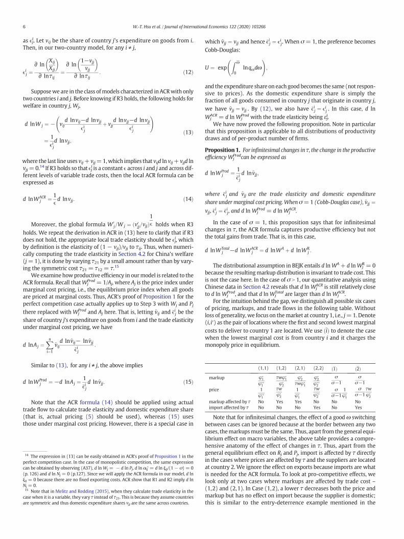
No Yes Yes No No No port affected by τ No No No Yes No Yes im
Note that for infinitesimal changes, the effect of a good ω switchingbetween cases can be ignored because at the border between any twocases, themarkupsmust be the same. Thus, apart from the general equi-librium effect on macro variables, the above table provides a compre-hensive anatomy of the effect of changes in τ. Thus, apart from thegeneral equilibrium effect on Rj and Pj, import is affected by τ directlyin the cases where prices are affected by τ and the suppliers are locatedat country 2. We ignore the effect on exports because imports are whatis needed for the ACR formula. To look at pro-competitive effects, welook only at two cases where markups are affected by trade cost –(1,2) and (2,1). In Case (1,2), a lower τ decreases both the price andmarkup but has no effect on import because the supplier is domestic;this is similar to the entry-deterrence example mentioned in the


introduction. In Case (2,1), a lower τ increases themarkup but does notaffect the price and import because the foreign supplier is constrainedonly by the domestic best. Thus, in cases where markups are affectedby τ, imports are unaffected. If the expenditure share of each case is un-affected by small changes in τ, then the welfare impacts of τ viamarkups are totally independent of imports (Proposition 1). The reasonwhy Proposition 1 need not hold under σ N 1 is that changes in tradecost τ may change the expenditure shares across goods and henceacross different cases. Nevertheless, it will be seen in the quantitativeanalysis in Section 4.2 that the effects due to changes in expenditureshare are minor, as the extra gains from trade over the ACR formula re-main roughly those due to pro-competitive effects.

In sum, Proposition 1 and the above table show how head-to-headcompetition separates markups and trade flows, and hence make thetotal welfare gains from trade in our model different from the ACR for-mula. In contrast, the total gains from trade in EMX can be capturedby the ACR formula because even with finite number of firms, eachfirm owns a variety and hence a demand curve along which the pricingis determined, taking into account strategic interactions among firms. Achange in τ changes the foreign supplier’s delivered marginal cost, andtherefore changes the price, markup, and import simultaneously. Simi-larly, even though the ACR formula must be modified in Arkolakis et al.(2019) to account for the change from CES preference to a general pref-erence that allows variable markup, the fact that each firm owns a vari-ety under monopolistic competition still makes trade flows sufficientstatistics for welfare gains from trade.

3. Quantifying the Model

As the markup distribution is the central focus of the paper, our ap-proach of quantifying the model relies heavily on the distribution ofmarkups, which is estimated from the Chinese firm-level data. Notethat unlike EMX whose benchmark focuses on symmetric countries,our empirical implementation focuses on asymmetric countries, as thelarge wage gap between China and the ROW should not be ignoredsince it may have a large impact on parameter estimates, as well as po-tential large general equilibrium effects in counter-factuals. Despite thelack of firm level data in the ROW, we demonstrate that separatingmo-ments of exporters and nonexporters can help identify the different pa-rameters of the two countries. In this subsection, we first describe thedata and approach by which our model is quantified. We then presentand discuss the estimation results, and make a comparison with theBEJK model.

17 We also conduct estimation and counter-factual analysis under raw markups as a ro-bustness check.18 In our implementation of the DLW approach using Chinese firm-level data under thetranslog production function, which allows variable returns to scale, it turns out that thereturns to scale are quite close to constant. See Panel B of Table A1 in Appendix A1. Inter-estingly, EMX also found similar results using Taiwanese firm-level data.19 Following the literature, e.g., De Loecker et al. (2016) and Lu and Yu (2015), we trim

3.1. Data

Our firm-level data set comes from the Economic Census data (1995and 2004) from China’s National Bureau of Statistics (NBS), whichcovers all manufacturing firms, including SOEs. The sample sizes for1995 and 2004 are 458, 327 and 1, 324, 752, respectively.16 The advan-tage of using this data set, instead of the commonly used firm-level sur-vey data set, which reports all SOEs and only those private firms withrevenues of at least 5 million renminbi, is that we do not have to dealwith the issue of truncation. As we are concerned with potential re-source misallocation between firms, it is important to have the entiredistribution. We estimate the models separately for the years 1995and 2004.

We obtain world manufacturing GDP and GDP per capita from theWorld Bank’sWorld Development Indicators (WDI). The aggregate Chi-nese trade data is obtained from the UN COMTRADE.

16 The original data sets have larger sample sizes, but they also include some (but not all)non-manufacturing industries, as well as firms without independent accounting and vil-lage firms, which entail numerous missing values. The final sample is obtained after ex-cluding these cases and adjusting for industrial code consistency.

3.2. Estimation of Markups

Under the constant returns to scale assumption, a natural way toestimatemarkups is by taking the ratio of revenue to total costs, i.e., rev-enue productivity, orwhatwe call rawmarkup. However, it is importantto recognize that, in general, raw markups may differ across firms, notonly because of the real markup differences, but also because of differ-ences in the technology with which they operate. To control for this po-tential source of heterogeneity, we usemodern IOmethods to purge ourmarkup estimates of the differences in technology. In particular, we es-timatemarkups following DLW’s approach,17 who calculatemarkups as

mω ¼ θXωαXω;

where θωX is the input elasticity of output for input X, and αωX is the share

of expenditure on input X in total revenue. Tomap our model into firm-level data, we relax the assumptions of a single factor of production andconstant returns to scale. FollowingDLW,we assume a translog produc-tion function.18 The estimation of firm-levelmarkup hinges on choosingan input X that is free of any adjustment costs and the estimation of theelasticity of output to this input, θωX . As labor is largely not freely chosenin China (particularly SOEs) and capital is often considered a dynamicinput (whichmakes its input elasticity difficult to interpret), we chooseintermediate materials as the input to estimate firm markup (see alsoDLW). The full details of themarkup estimation are relegated to Appen-dix A1.

Table 1 gives summary statistics of the markup distribution,19 withbreakdowns in each year and between exporters and non-exporters.Observe that the (unweighted) mean markups all decrease between1995 and 2004 for all firms, both exporters and non-exporters. The(unweighted) standard deviation of markups decreases for non-exporters, but increases slightly for exporters. Because there are morenon-exporters than exporters and the decrease in the standard devia-tion of non-exporters is larger than the increase in the standard devia-tion of exporters, the overall standard deviation decreases. Almost allof the percentiles decreased between 1995 and 2004. This is consistentwith the pattern seen in Figure 1 where the entire distribution becomesmore condensed.

However, we note that the pattern described in Table 1 only hints atthe existence of pro-competitive effects. The reduction of dispersion offirm markups does not necessarily mean that the allocative efficiencyincreases, as allocative efficiency depends on consumer markups ratherthan firm markups. It does show that the markets facing Chinese firmsbecame more competitive. Also, we cannot reach a conclusion yetabout the relative markup effect, as we do not observe the consumers’aggregatemarkup directly.We need to quantify themodel and simulateboth types of markups to conduct welfare analysis.

3.3. Simulated Method of Moments

3.3.1. MethodGiven measures of {w,R1,R2}, we use moments of markups, trade

flows, number of firms and fraction of exporters to estimate all param-eters except L2/L1 by SMM. We estimate the parameters using SMM for

the estimated markup distribution in the top and bottom 2.5 percentiles to alleviate theconcern that the extreme outliers may drive the results. Our results are robust to alterna-tive trims (e.g., the top and bottom 1%; results are available upon request). We also dropestimated markups that are lower than one, as our structural model does not generatesuch markups.

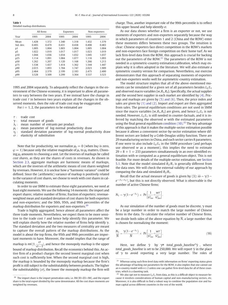
Table 1Detailed markup distributions.

All firms Exporters Non-exporters

Year 1995 2004 1995 2004 1995 2004

Mean 1.428 1.372 1.340 1.318 1.432 1.379Std. dev. 0.495 0.479 0.431 0.438 0.498 0.483p1 1.005 1.004 1.003 1.004 1.005 1.004p5 1.022 1.019 1.017 1.017 1.023 1.019p10 1.044 1.036 1.034 1.032 1.045 1.037p25 1.114 1.091 1.084 1.077 1.116 1.093p50 1.262 1.207 1.120 1.168 1.266 1.213p75 1.538 1.437 1.414 1.362 1.544 1.447p90 2.015 1.893 1.784 1.747 2.023 1.909p95 2.464 2.379 2.199 2.183 2.475 2.400p99 3.528 3.509 3.299 3.364 3.537 3.523

21 Whereas using such firm-level data with information on firms’ exporting status givesthe advantage of backing out parameters for the ROW, it also implies that one cannot usean n-country model with n ≥ 2 unless one can gather firm-level data for all of these coun-tries, which is a daunting task.


1995 and 2004 separately. To adequately reflect the changes in the en-vironment of the Chinese economy, it is important to allow all parame-ters to vary between the two years. If we instead have the change intrade cost τ in between two years explain all the changes in the ob-served moments, then the role of trade cost may be exaggerated.

For i = 1, 2, the parameters to be estimated are

τ : trade costγ : total measure of goodsλi : mean number of entrants per productμ i : mean parameter of log‐normal productivity drawηi : standard deviation parameter of log‐normal productivity drawσ : elasticity of substitution

Note that for productivity, we normalize μ2 = 0 (when lnφ is zero,φ = 1) because only the relative magnitude of μ1 to μ2 matters. Choos-ing μ2 amounts to choosing a unit. Let the inverses of markups be calledcost shares, as they are the shares of costs in revenues. As shown inSection 2.3, aggregate markups are harmonic means of markups,which are the inverses of the arithmetic means of cost shares weightedby revenues. However, it is unclear how a “harmonic variance” could bedefined. Since the (arithmetic) variance of markup is positively relatedto the variance of cost shares, we choose toworkwith cost shares in cal-culating moments.

In order to use SMM to estimate these eight parameters, we need atleast eightmoments.We use the following 14moments: the import andexport shares; relative number of firms; fraction of exporters; revenue-weightedmean and standard deviation of cost shares for both exportersand non-exporters; and the 50th, 95th, and 99th percentiles of themarkup distribution for exporters and non-exporters.20

Trade is highly aggregated; hence almost all parameters affect thethree trade moments. Nevertheless, we expect them to be more sensi-tive to the trade cost τ and hence help identify this parameter. Wewill explain shortly how the relative number of firms help identify γ.The standard deviation and the two measures of centrality are meantto capture the overall pattern of the markup distributions. As themodel is about the top firms, the 95th and 99th percentiles are impor-tant moments to have. Moreover, the model implies that the range of

markup is m∈½1; σσ−1

�, and hence the monopoly markup is the upper

bound of markup distribution. Recall the economics behind this. An ac-tive firm of a product charges the second lowest marginal cost whensuch cost is sufficiently low. When the second marginal cost is high,the markup is bounded by the monopoly markup because the firm’sprofit is still subject to the substitutability between products. The higherthe substitutability (σ), the lower the monopoly markup the firm will

20 The import share is the import penetration ratio, i.e. IM/(R1-EX+IM), and the exportshare is the total export divided by the same denominator. All the cost sharemoments areweighted by revenues.

charge. Thus, another important role of the 99th percentile is to reflectthis upper bound and help identify σ.

As our data shows whether a firm is an exporter or not, we usemoments of exporters and non-exporters separately because the wayin which parameters of countries 1 and 2 (China and the ROW) enterthese moments differs between these two groups. The intuition isclear: Chinese exporters face direct competition in the ROW’s marketsand non-exporters face foreign competition on their home turf. As welack firm-level data from the ROW, this approach is crucial for backingout the parameters of the ROW.21 The parameters of the ROW is notneeded in a symmetric-country estimation/calibration, which may ex-plain why it is often adopted in the literature. We will also estimate asymmetric country version for comparison. Nevertheless, our exercisedemonstrates that this approach of separating moments of exportersand non-exporters works well for asymmetric-country estimation.

The model structure implies that all of the above-mentioned mo-ments can be simulated for a given set of all parameters besides L2/L1and observedmacro variables {w,R1,R2}. Specifically, the actual supplierand the second best supplier in each market are identified by (4). Pric-ings and markups are given by (5) and (6). Then, the price index andsales are given by (1) and (2). Import and export are then aggregatedfrom sales. The general equilibrium conditions are not used in SMMsince the macro variables {w,R1,R2} are given, and hence L2/L1 is notneeded. However, L2/L1 is still needed in counter-factuals, and it is in-ferred by matching the observed w with the estimated parametersusing the final general equilibrium condition (10).22 The key advantageof this approach is that it makes themultiple-sector estimation possiblebecause it allows a convenient sector-by-sector estimation where dif-ferent sectors are linked by a Cobb-Douglas utility function. There are29manufacturing sectors in China, and each sector carries 8 parameters.If one were to also include L2/L1 in the SMM procedure (and perhapsuse observed w as a moment), this implies the need to estimate29 × 8 + 1 = 233 parameters simultaneously in an over-identified es-timation with w computed as a general equilibrium object. This is notfeasible. For more details of the multiple-sector estimation, see Section5.1. Note that the model simulated R2/R1 is generally different fromthe data ones. We will check the external validity of our approach bycomparing the data and simulated R2/R1.

Recall that the actual measure of goods is given by (3): ω ¼ γ½1−e−ðλ1þλ2Þ�, but this is not directly observed. What is observable is thenumber of active Chinese firms:

N1 ¼ γ 1−e−λ1� �� Pr

1φ�1ω

bwτφ�2ω

� :

As our simulation of the number of goods must be discrete, γ mustbe a large number in order to match the large number of Chinesefirms in the data. To calculate the relative number of Chinese firms,we divide both sides of the above equation by N, a large number thatis chosen for normalizing the moment:

N1

N¼ γ 1−e−λ1

� �N

� Pr1

φ�1ω

bwτφ�2ω

� : ð16Þ

Here, we define ~γ by γ≡ total_goods_baseline*~γ , wheretotal_goods_baseline is set to be 250,000. We will report ~γ in the placeof γ to avoid reporting a very large number. The roles of

22 We also opt not to measure L2/L1 from data, as this is a difficult object to measure be-cause it involves considerations of human capital and non-manufacturing sectors, etc.Moreover, it is also difficult to find a robust way to combine the population size and hu-man capital across different countries in the rest of the world.

Table 2SMM results.

1995 2004

Predeterminedw Relative wages (the ROW to China) 10.25 5.18R1 China's manufacturing sales ($b) 918,291 2,343,328R2 ROW's manufacturing sales ($b) 9,397,500 14,737,500

Moments for SMM Data Model Data ModelImport share 0.130 0.148 0.222 0.252Export share 0.153 0.176 0.249 0.273Relative number of firms 0.210 0.193 0.596 0.605Fraction of exporters 0.044 0.023 0.105 0.064Mean cost share for exporters 0.845 0.802 0.801 0.789Std of cost share for exporters 0.135 0.135 0.142 0.139p50 markup for exporters 1.196 1.207 1.168 1.224p95 markup for exporters 2.199 2.173 2.183 2.207p99 markup for exporters 3.299 3.202 3.364 3.225mean cost share for non-exporters 0.789 0.715 0.829 0.763std of cost share for non-exporters 0.147 0.185 0.139 0.161p50 markup for non-exporters 1.266 1.383 1.213 1.285p95 markup for non-exporters 2.475 2.752 2.400 2.193p99 markup for nonexporters 3.537 3.202 3.523 2.735

Parameter values Estimates s.e. Estimates s.e.τ, trade cost 2.311 0.027 1.782 0.007γ, measure of goods relative tototal_goods_baseline

0.186 0.002 0.659 0.003

λ_1, Poisson parameter, China 2.455 0.037 2.618 0.017λ_2, Poisson parameter, ROW 5.535 0.037 5.024 0.048μ_1, mean of log productivity, Chinarelative to ROW

−2.397 0.023 −1.756 0.012

η_1, std of log productivity, China 0.450 0.004 0.425 0.002η_2, std of log productivity, ROW 0.351 0.022 0.357 0.011σ, elasticity of substitution 1.454 0.003 1.449 0.003

Simulated R2/R1 Data Model Data ModelR2/R1 10.234 9.388 6.289 5.875

Notes: All units, if any, are in billions USD, current price. The import share is the importpenetration ratio, i.e. IM/(R1-EX+IM), and the export share is the total export dividedby the same denominator. All the cost share moments are weighted by firms' revenues.Recall that a firm's cost share is the inverse of its markup. p# denotes the #-th percentile.


total_goods_baseline and N are different. The former affects how precisea simulation is; the larger the total_goods_baseline, the more goods andfirms there are and hence the more precise a simulation will be. Theconstant N is only for normalization and does not affect the estimates.23

How the macro variables {w,R1,R2} are obtained from data is as fol-lows. To calculate w = w2/w1, we first obtain the GDP per capita ofChina and the ROW from WDI.24 We then proxy wi by multiplyingGDP per capita by the labor income shares for the ROW and China,which are taken from Karabarbounis and Neiman (2014).25 For R1 andR2, we first obtain the manufacturing GDPs of China and the ROWfrom WDI data. We then use the input-output table for China (2002)and the US (1997–2005) to obtain GDP’s share of total revenue. Wethen use such shares and the manufacturing GDPs to impute R1 and R2as total revenue. Although our model does not distinguish valueadded and revenue, we choose to interpret Ri as total revenue ratherthan GDP to be consistent with our export and import moments,which are also in terms of revenue.

We use the equal-weight weighting matrix in our SMMimplementation.26 The nature of themoments implies that someempir-ical moments, e.g., mean and standard deviation of cost shares, wouldbe estimated more accurately than others, e.g., the top quantiles ofmarkups. Thus, under the optimal weighting matrix calculated fromthe inverse of the variance-covariancematrix of the empiricalmoments,those top-quantile moments would tend to have smaller weights. How-ever, these top-quantile moments are crucial in identifying key modelparameters (λi, ηi, σ) as explained in Section 3.3.2 below, and thus wechoose to treat each moment equally in our estimation procedure. Thestandard errors are calculated by the standard approach as in Addaand Cooper (2003, p. 88). As will be seen shortly, the standard errorsin our implementation tend to be rather small due to the large samplesizes.

3.3.2. SMM ResultThe estimation result is shown in Table 2. The model fits the data

moments reasonably well, and the small standard errors indicate thateach parameter is relatively precisely estimated. The bottom row re-ports data and model simulated R2/R1, and they turn out to be reason-ably close, serving as additional validation of the model.

As we estimate the models for 1995 and 2004 separately, thechanges of the parameters are strikingly consistent with well-knownempirical patterns about the Chinese economy during this period.From 1995 to 2004, the estimate of τ shows a dramatic decrease from2.31 to 1.78. The measure of goods γ more than triples from 0.19 to0.66. This basically reflects the sharp increase in the number of firms be-tween the two Economic Censuses, from 458,327 in 1995 to 1,324,752in 2004, which is almost triple. The mean number of entrants per prod-uct in China (λ1) increased from 2.46 to 2.62, whereas in the ROW it de-creased from 5.54 to 5.02. China’s mean log productivity (μ1) relative tothe ROW increased from −2.40 to−1.76. These numbers are negative,meaning that China’s productivity is lower than that of the ROW. Also,we see a slight decrease (increase) in the dispersion parameter of theproductivity distribution in China (ROW). Interestingly, the

23 We set N ¼ 2;000;000 so that the relative numbers of firms are 0.210 and 0.596 in1995 and 2004, respectively. We initially set total_goods_baseline to 2,500,000. However,we find that the calculated moments under total_goods_baseline=250,000 are virtuallythe same as those under 2,500,000. For faster computing speed, we thus settotal_goods_baseline=250,000. To fit the above-mentioned relative numbers of firms(the left-hand side of [16]) in the SMM procedure, we set N ¼ 200; 000 so that we effec-tively scale both the numerator and denominator of the right-hand side of (16) by 1/10.24 The ROW’s GDP per capita is the population-weighted average of GDP per capitaacross all countries other than China.25 The ROW’s labor share is the weighted average of labor share across all countries be-sides China, with the weight being relative GDP.26 Specifically, this weighting matrix is the inverse of the diagonal matrix with each di-agonal element being the square of eachdatamoment. This is equivalent to using the iden-tity matrix if the moment error is first normalized by the data moment. Normalization isneeded because themagnitudes of the data moments vary substantially from 0.13 to 3.54.

productivity dispersion is larger in China than in the ROW, which isconsistent with the finding by Hsieh and Klenow (2009).27

The σ estimate we obtain is approximately 1.45 in both years.28 Thisestimate is quite low comparedwith those estimates inmodels that fea-ture constant markups (often a CES preference coupledwith either mo-nopolistic competition or perfect competition), and this is drivenmainlyby the need to fit the two 99th percentiles in the markup distribution.Recall that σ/(σ − 1) in our model is the upper bound rather than theaverage ofmarkups. Under a constant-markupmodel and using thehar-monic mean of firm markups in 1995, 1.259, this implies σ = 4.86.However, in the current model, this value of σ implies that m ∈[1,1.259], which cuts 50.6% off the estimated markup distribution.Then, these large markups where most distortions come from are ig-nored. In fact, the pro-competitive effects of trade become negligibleunder m ∈ [1,1.259] because the associated allocative efficiency ismuch closer to the first-best case (constant markup) without the veryskewed larger half of the markups. EMX also found that the extent ofpro-competitive effects depends largely on the extent to whichmarkups can vary in themodel. In fact, our estimate is strikingly similar

27 The mean of a log-normal distribution is eμ+η2/2. According to our estimates of μ1 andη1 in these two years, this translates to an annual productivity growth rate of 7.25%. Thisimpressive growth rate is actually similar to the 7.96% estimated by Brandt et al. (2012).Note that the 7.25% growth rate here is relative to the ROW. If the ROW also grows in theirproductivity, the actual productivity growth rate could be even higher. In fact, Brandt et al.(2017) find a 12% average TFP growth rate at industry level. The data used in both above-mentioned papers is the annual manufacturing survey data from 1998 to 2007.28 Note that this estimate ofσ is not sensitive to sample size. In ourmulti-sector exercise,the unweighted means of σs are 1.56 and 1.53 for 1995 and 2004, respectively, and 24 ofthe 29σs arewithin one standard deviation from themean in both years. See Section 5.1.4.

Table 3Jacobian matrix.

Moments τ γ λ_1 λ_2 μ_1 η_1 η_2 σ

Import share −0.409 0.005 −0.072 0.001 0.251 −0.019 0.554 −0.030Export share −0.742 0.003 0.082 −0.101 0.966 0.665 −0.204 −0.026Relative number of firms 0.252 0.971 0.102 −0.015 0.429 0.179 −0.769 0.000Fraction of exporters −0.167 0.001 0.006 −0.018 0.130 0.167 0.012 0.000Mean cost share for exporters −0.031 −0.001 0.023 0.012 0.040 −0.140 −0.034 0.021Std of cost share for exporters 0.022 0.003 −0.016 −0.016 −0.041 −0.152 0.062 −0.050p50 markup for exporters 0.055 −0.006 −0.033 −0.016 −0.052 0.269 0.010 0.006p95 markup for exporters 1.597 −0.408 −1.949 −0.556 −2.088 −13.072 1.419 −0.070p99 markup for exporters 0.000 0.000 0.000 0.000 0.000 0.000 0.000 −5.107Mean cost share for non-exporters −0.088 −0.003 0.021 0.002 −0.063 −0.360 0.089 0.014Std of cost share for non-exporters 0.054 0.003 −0.008 −0.001 0.030 0.175 −0.023 −0.010p50 markup for non-exporters 0.154 0.011 −0.044 −0.005 0.141 0.639 −0.173 0.000p95 markup for non-exporters 0.929 −0.004 −0.159 −0.027 0.660 2.973 −0.480 0.000p99 markup for non-exporters 1.914 0.055 −0.205 −0.067 0.880 3.636 −0.491 −0.877

Notes: Each entry of this table gives the rate of change of amoment to a parameter. This is based on the benchmark estimation of the 2004model. The larger the absolute value of the rate ofchange, the more sensitive this moment is to the parameter, and the more useful this moment is in identifying this parameter.


to the estimate of the same parameter (1.37) in Simonovska andWaugh(2014) with the optimal weighting matrix in their method of momentsprocedure.

Note that in BEJK, the trade elasticity is given by the tail index of theFréchet distribution, and is independent of the elasticity of substitutionσ. In our model where the productivity draws deviate from Fréchet, σmay potentially matter in determining trade elasticity, but the effectseems small, as we will see in Section 4.2 that the trade elasticities inour model are quite close to those found by Simonovska and Waugh(2014) under the BEJK model.

Based on the 2004 estimation, we calculate a Jacobian matrix inwhich each entry gives a rate of change of a moment to a parameter;this is shown in Table 3. The larger the absolute value of a rate of change,themore sensitive thismoment is to the parameter, and hence themoreuseful this moment is in identifying this parameter, at least at the localarea of the optimal estimates. With such Jacobian matrices, the asymp-totic variance-covariance matrices of the optimal estimates can be cal-culated to produce the standard errors reported in Table 2.

It is obvious from Table 3 that σ is almost single-handedly deter-mined by the 99th percentile of markups for exporters, and this mo-ment has little influence on other parameters. Trade cost τ affectsalmost all moments significantly except the 99th percentile of markupsfor exporters. It is natural to see that the two trade moments, the rela-tive number of Chinese firms and the fraction of exporters are particu-larly strong for identifying this. Interestingly, when τ increases, the95th percentiles of markups for both exporters and non-exporters, aswell as the 99th percentile of markups for exporters, increase sharply.For non-exporters, this is intuitive because a higher τ provides non-ex-porters more insulation from foreign competition, and the top non-ex-porters gain more from this. For exporters, a higher τ makes it harderfor them to compete in foreign markets, but recall that an exporter’smarkup is a harmonic mean of the markups in both the domestic andforeignmarkets. Itmust be that the gains inmarkups at home outweighthe losses in markups in foreign markets.

For the identification of λ1, the top percentiles of markups play thedominant role. The intuition is as follows. Fixing other parameters,when λ1 increases, the number of entrants per product in China in-creases. Due to the non-fat-tailed nature of the productivity distribu-tion, the ratio between the top two draws is narrowed, but since thisratio is indeed the markup and since this is particularly pronouncedfor the top markups, the top percentiles are particularly useful in iden-tifying this parameter. The relative number of firms also plays somerole, as (16) shows that the larger the λ1, the larger the probabilitythat China draws a positive number of firms from the Poisson distribu-tion. For λ2, the 95th percentile of markups for exporters and the exportshare are the key moments. A larger λ2 implies fiercer competition onthe foreign turf for exporters as it brings out better competitors from

the ROW, reducing both China’s export share and the 95th percentileof markups for exporters.

For the measure of goods γ, the relative number of Chinese firms isthe most useful moment. An increase in mean productivity parameterμ1 increases export share, the number of Chinese firms, and the fractionof exporters, but decreases the import share. These are all intuitive.However, an increase in μ1 sharply increases the 95thpercentilemarkupfor non-exporters but sharply decreases the 95th percentile markup forexporters. This is because top non-exporters are actually not the mostproductive firms – their productivities are somewhere in the middleof the distribution and hence they gain inmarkup by having higher pro-ductivity. In contrast, top exporters are the most productive firms, andthey lose in markup when they become even more productive, due tothe compression at the upper tail of the productivity distribution.

For η1 and η2, first note that they are not only dispersion parameters,but their increases induce increases in means as well. Hence, the direc-tion of changes due to a change in η1 is similar to that of a change in μ1,but the intensities are quite different. For example, η1 has much largereffects on almost all moments of markups than μ1, but it has smaller im-pacts on the trade moments. In particular, the 95th percentile markupfor exporters is extremely sensitive to η1 because η1 affects the top pro-ductivities muchmore than μ1. Also note the interesting pattern: η1 andη2 affect many moments in opposite ways. An increase in η2 increasesboth the mean and dispersion of the ROW’s productivity, and this in-creases China’s import share, and decreases China’s export share andnumber of firms. It compresses the markup distribution of non-ex-porters, but it increases the 95th percentile of markups for exporters.

Finally, we discuss a point that is often mentioned in studies of theChinese economy. China underwent various reforms, including but notlimited to trade reforms, in this decade. One notable reform is that ofSOEs during the late 90s,which iswell known to havemade China’s var-ious industries more competitive. Althoughwe do notmodel the sourceof distortion explicitly in ourmodel and rather treat markups (and theirdistribution) as a reflection of distortion, the fact that we observe in-creases in both λ1 and γ may be partly due to these reforms. The com-pression in markup distribution (Table 1 and Figure 1) and theincreasing number of manufacturing firms are also consistent with theabove-mentioned reforms.

3.4. Comparison with the BEJK Model

Asmentioned, there are no pro-competitive effects and the ACR for-mula is satisfied in the BEJK model. A natural question is whether ourmodel fits the data better than the BEJKmodel, at least for some aspectsof data patterns. This question is important because if the BEJK modeldominates our model in almost all aspects of data patterns, then onemay be less interested in our welfare analysis. To examine this, we

t

Table 4Counter-factual analysis.

Panel A: Counter-factual from 2004 estimates

Under 2004Estimates τ at 1995 % change Autarky % change

τ, trade cost 1.782 2.311 1,000,000

WelfareTotal welfare 2.12E+12 1.98E+12 7.1% 1.66E+12 28.0%W_Prod 2.21E+12 2.09E+12 5.6% 1.83E+12 20.7%W_A 0.958 0.944 1.5% 0.904 6.0%W_R 1.000 1.000 -0.1% 1.000 0.0%

Contribution to total welfareW_A and W_R 19.9% 21.5%W_A 20.6% 21.6%

Panel B: Counter-factual from autarky

Autarky

10%importshare

% changefromautarky

20%importshare

% change from10% importshare

τ, trade cost 1,000,000 2.424 1.916

WelfareTotal welfare 1.66E

+121.96E+12

18.4% 2.07E+12

5.6%

W_Prod 1.83E+12

2.08E+12

13.6% 2.17E+12

4.2%

W_A 0.904 0.942 4.2% 0.954 1.3%W_R 1.000 1.000 0.0% 1.000 0.0%

Contribution to total welfareW_A and W_R 23.1% 23.5%W_A 22.9% 24.2%

Notes: In Panel A, all the analysis is done under 2004 estimates, and only the trade cost (τ)changes. The reported percentage changes in this panel are under the changes from thecorresponding τ to 2004's τ. Panel B reports results when τ is changed from an inhibitivelevel (autarky) to the level that entails 10%, and then from 10% to 20%, with other param-eters fixed at the 2004 estimates.

29 Observe that the cost andprice channels have two sets in common; the only differenceis that the cost channel has the case (2,1) whereas the price channel has the case (1,2).Again, the fact that domestic firms need not pay trade costs compared with foreign firmsimplies that the averagemarkup in the case (1,2) is high comparedwith that in case (2,1)and the overall average, and thus Emb EmΩp↑. The Frechét structure inBEJK implies that theselection force introduces sufficiently productive foreign firms, and thus depresses themarkups in case (1,2) so that Em= EmΩp↑. But this is not the case under log-normal pro-ductivity draws.


conduct two sets of comparisons. The first set is to fit the BEJKmodel bySMM to the above-mentioned moments that discipline our estimationand then compare with our benchmark result from Table 2. The secondset is to addmoments that BEJKwere concernedwithmatching and useSMM to estimate both the BEJK and our model. We find that our modelfits better than the BEJKmodel in both sets of comparison. The details ofthe comparison are given in Appendix A2.

4. Gains from Trade

In this section, we conduct a battery of counter-factual analyses toexamine the welfare gains from trade.

4.1. Welfare Analysis: Between 1995 and 2004 and from Autarky

To examine gains from trade, we conduct two counter-factual anal-yses byfixing all parameter values at the 2004 level and changing only τ.In the first analysis, we simulate welfare and its components when τ ischanged to the 1995 level, and we calculate the percentage changes ofwelfare and its components. In the second analysis, we take τ to a pro-hibitive value so that the economy goes to autarky.

The results are shown in Table 4. The welfare gains of changing τfrom 1995’s level to 2004’s level are 7.1%, in which allocative efficiencyaccounts for 20.6% (1.5/7.1) and relative markup effect accounts for−0.7%. Thus, these pro-competitive effects jointly account for 19.9% ofthe total gains from trade. In fact, both aggregate markups Msell andMbuy decrease during this period, which is a natural result under tradeliberalization, but the percentage decrease in the consumers’ aggregatemarkup Mbuy is smaller. Overall, although the relative markup effect isnegative, it is relatively small, whereas the combined effect can accountfor about one fifth of the total gains. The total gains from autarky to2004’s τ are, of course, much larger, at 28%, but the decomposition issimilar to the first analysis.

To understand the intuition behind the gains due to allocative effi-ciency, we follow Holmes et al. (2014) to distinguish markup changesby a cost channel and a price channel. An increase in τ increases mar-ginal costs proportionately in events (2,1), (2,2), and ð2Þ as defined inSection 2.6. This channel reduces markups when prices are held fixed.An increase in τ increases prices proportionately in events (1,2), (2,2),and ð2Þ and markups when costs are held fixed. From country 1’s view-point, Holmes et al. show that

ηA ≡d lnWA

d lnτ¼ ηAcost þ ηAprice� �d ln τwð Þ

d lnτ; ð17Þ

where

ηAcost ¼ s2Emσ−1

2

Emσ−1 −EmEm2

!; ð18Þ

ηAprice ¼ −σsΩp↑ 1−Em

EmΩp↑

� �: ð19Þ

Here, E is the revenue-weighted harmonic expectation operator, andthus Em is actually the consumers’ aggregatemarkupMbuy as defined ear-lier. Also, s denotes an expenditure share, and the subscript 2 denotes theset of imported goods (from country 2), which also represents the costchannel. The subset Ωp↑ is the set of goods affected by the price channel.

As the general equilibrium effect term d ln (τw)/d ln τ is generallypositive, the sign of the allocative efficiency hinges on the signs of ηcosA

and ηpriceA . Both terms are negative under the 1995 and 2004 estimates,implying positive allocative efficiency gains when trade costs reduce.More specifically, the mean markup of imported goods Em2 is lowerthan that of all goods (so that Em/Em2 N 1 N Em2

σ−1/Emσ−1).When pricesare held fixed, a trade liberalization reduces costs and increases

markups of imported goods, reducing the discrepancy between Em2

and Em and mitigating distortion. Similarly, a trade liberalization de-creases prices and markups through the price channel. Under our esti-mates, EmΩp↑ is greater than Em, and thus a trade liberalization reducesmarkup dispersion and distortion through the price channel, too.

The key of the above discussion is that Em2 b Em b EmΩp↑ under ourmodel and estimates. In the BEJKmodel, Em2= Em because themarkupdistribution conditional on the source is actually independent of thesource. Hence, the cost channel disappears (ηcostA = 0). As the markupdistribution in any country is invariant to trade costs, ηcostA + ηpriceA =0, and thus ηpriceA = 0. Foreign firms selling to China need to pay tradecosts that domestic firms avoid. Other things being equal, this drivesup the costs and lowers the markups of foreign firms so that Em2 b

Em. However, there is also a selection of productivities that only rela-tively productive foreign firms can export, and this tends to increasemarkups of foreign firms. This latter force critically depends on theupper tail of the productivity distribution. Under the Fréchet structurein BEJK, this force is so strong that the two forces exactly counterbal-ance, entailing Em2= Em. In contrast, the selection force is not as strongwith log-normal productivity draws in our model, and thus Em2 b Em.The intuition for why Em b EmΩp↑ is similar.29


Next, we examine whether the result of “diminishing returns inopenness” in EMX holds here. The following table summarizes the wel-fare gains reported in their study, as well as the breakdown in Ricardiangains and allocative efficiency. There is an obvious “diminishingreturns” in allocative efficiency, as the opening up from autarky to 10%import share improves welfare by 1.2%, whereas further opening upfrom 10% to 20% improves welfare by only 0.3%. But such adiminishing-returns pattern does not show up in the Ricardian compo-nent. As a result, the contribution of allocative efficiency diminishes rap-idly from 1.2/3.1 ≈ 38% to 0.3/2.8 ≈ 10.7%.

3

se−th3

Import share

0

0 Here, we set wecant error in calculf(x− h)]/2h, wheree trade elasticity ε121 See Tables 4 and

%Δ in EMX

set h = 0.0001, and thus τ′ is about 0.1%ating trade elasticity, we use two-point formux= ln (τ21) and f= ln ((1− v11)/v11). Note

, wages are taken as fixed, as in ACR.7 in their paper.

Importance of WA

Total welfare
Ricardian WA
–10%
3.1 1.9 1.2 38.7% 0%–20% 2.8 2.5 0.3 10.7% 1
Panel B of Table 4 reports the result from a similar exercise. Note thatEMX’s pro-competitive effect includes only allocative efficiency but notthe relative markup effect, as their formulation focuses on symmetriccountries. To compare, we ignore the relative markup effect. A similardiminishing returns pattern in allocative efficiency is obvious, droppingfrom 4.2% to 1.3%. But, unlike in EMX, we also see sharp diminishingreturns in our counter-factuals for total welfare and the Ricardian com-ponent. As a result, we do not see a diminishing contribution inallocative efficiency. Indeed, the contribution stays around 23%, whichis quite close to the results reported in Panel A.

Looking at both panels together, the contribution of pro-competitiveeffects ranges from 19.9% to 23.5%, and the contribution of allocative ef-ficiency ranges from 20.6% to 24.2%. Despite the differences in modelstructures, our estimates turn out to be in the ballpark of EMX’s esti-mates, which range from 11% to 38%.

t

4.2. Comparison with the ACR Formula

In this subsection, we compare the welfare gains in this model withthe ACR formula in two ways. First, we compare with the local ACR for-mula for small changes in trade cost. Second, as trade elasticity is a var-iable, the global ACR formula does not apply, but one can integrate thelocal formula to examine the gains from 1995’s τ to 2004’s τ in a similarfashion to Panel A of Table 4.

For the first comparison, recall from Section 2.6 that for the case of σ= 1 (Cobb-Douglas), the ACR formula captures the gains in productiveefficiency for small changes in trade costs, but not the total gains fromtrade. For general σ N 1, analytical results on the comparison with theACR formula are not available, and here we provide a quantitative anal-ysis based on the estimated models at 1995 and 2004. For this exercise,we investigate the effect of a small reduction h in the logarithm of tradecost so that lnτ′= ln (τ)− h. The results are reported in Table 5. Here,the welfare gains are expressed in terms of elasticity to trade cost, i.e.,d ln (W)/d ln τ, where W can be WTotal, WProd, WA × WR, or WACR. Asdiscussed in Section 2.6, the trade elasticity used in evaluating d lnWACR is ε12.30

The local trade elasticities in our estimated model in 1995 and 2004are−2.85 and −3.30, which are lower than standard estimates in theliterature but surprisingly close to the estimates of trade elasticityunder the BEJK model in Simonovska and Waugh (2014), which rangefrom −2.74 to −3.32.31 As explained by Simonovska and Waugh(2014), different micro mechanisms imply different distributions ofprice gaps of goods between countries. For example, price gaps are on

off τ. To reduce thela: f′(x) = [f(x + h)

that when calculating

average smaller in the BEJK model than those in the Eaton-Kortummodel. Tomatch the samemean price gap from the data, the productiv-ity dispersion needs to be larger in the BEJK model than the Eaton-Kortum one. This implies a smaller tail index of the Fréchet distributionand hence smaller trade elasticity in the BEJKmodel. The degrees of dis-persion in productivity, price gaps, and markups are all positively re-lated. Also, the differences in the moments of markups betweenexporters and non-exporters may play a similar role to the price gapsin Simonovska andWaugh (2014). Thus, to fit themoments ofmarkups,firm productivities in ourmodel also need to be sufficiently dispersed; itturns out the local trade elasticities in this model are close to theirestimates.

In 1995, thewelfare elasticity of trade cost is 0.249, meaning a 1% re-duction in trade cost τ induces a 0.249% increase in real income; 23.2% ofthis elasticity is from pro-competitive effects. The ACR formula entails awelfare elasticity of 0.190, which is quite close to the elasticity of pro-ductive efficiency 0.191. As a result, the totals gains from trade are largerthan the gains predicted by the ACR formula by 31.3%; most of theseextra gains are from pro-competitive effects. In the 2004 model, thecontribution of pro-competitive effects and the additional gains overthe ACR formula are smaller at 20.3% and 13.0%, respectively. Notethat the contributions of pro-competitive effects in Table 5 are still rel-atively similar in magnitude to those reported in Table 4.

Note that the total gains and their components (as point elasticities)are all larger in 2004 than in 1995. To understand why this is the case,we focus on the allocative efficiency first.We compute ηcostA and ηpriceA ac-cording to (18) and (19), and find that both ηcostA and ηpriceA are negative,implying positive allocative efficiency gains from a decrease in τ. The

ηAcost þ ηAprice ≡d lnWA

d lnðτwÞ term is −0.049 and −0.042 in 1995 and 2004,

respectively, but the general equilibrium term d ln (τw)/d ln τ is 1.18and 1.73, respectively. It is then clear that the allocative efficiencygains are larger in 2004 mainly because of the general equilibriumterm. Asw is 10.25 in 1995 (compared with 5.18 in 2004), a percentagedecrease in τ in 1995 can only induce a smaller percentage decrease inτw because w is large. Apart from the general equilibrium term, ηcosA

+ ηpriceA is smaller in 2004,which is in linewith the facts that theproduc-tivity distribution in China is less skewed in 2004 and that the differencein average productivity between China and the ROW has becomesmaller.

As the productive efficiency gains in our model approximate(roughly) the ACR gains, consider the ACR gains under symmetric coun-tries for clearer intuition. In this situation, the ACR formula becomes d lnWACR/d ln τ = − (1− v). The smaller the trade cost τ, the smaller thedomestic expenditure share v and the larger the ACR gains. Hence, theproductive efficiency gains is larger in 2004 mainly because the tradecost estimate τ is significantly lower in 2004 than in 1995.

For the second comparison, we integrate the local ACR formula tocomputewhat their formulawould predict for a change in trade cost be-tween 1995 and 2004’s levels. That is, we computeW1

ACR, 2004/W1ACR, 1995

lnWACR;2004

1

WACR;19951

¼Z τ2004

τ1995d lnWACR

1 τð Þ ¼Z τ2004

τ1995d

lnv11 τð Þϵ τð Þ

� �: ð20Þ

We relegate the calculation details to Appendix A3. The result is thatthe gains from trade according to the ACR formula are 5.9%. The totalgains from trade 7.1% (Table 4) are 20.3% higher than the ACR formula.

In the benchmark exercise, the overall gains at 7.1% seems a rela-tively large number compared with those found in the literature. Thesources of the larger gains compared with the literature are three-fold.The first source is the large reduction in trade cost, which is essentiallyinferred by the large increases in tradeflows and the fraction of exporterduring 1995–2004. This means wider bounds of integration in (20). If

the trade elasticity were a constant, (20) would reduce to W ¼ v1=ϵ ,and the large change in trade cost would imply a low value of v. Second,

Table 5Welfare analysis local to the estimated model and comparison with the ACR formula.

Total welfaregains

Gains in productiveefficieny

Pro-competitivegains

Contribution of pro-competitiveeffects

Tradeelasticity

Gains by the ACRformula

Additional gains over the ACRformula

1995 0.249 0.191 0.058 23.2% −2.85 0.190 31.3%2004 0.362 0.289 0.073 20.3% −3.30 0.320 13.0%

Notes: All thewelfare gains here are calculated in terms ofwelfare elasticity to trade cost, i.e., dln(W)/dln(τ), whereW could be totalwelfare or its components, or the one according to theACR formula. For both the 1995 and 2004 models, we calculate the welfare gains and its components from estimated tau to the case where ln(tau')=ln(tau)-h, where h = 0.0001. Toreduce secant error in calculating trade elasticity, we use two-point formula: f'(x)= (f(x+h)-f(x-h))/2h, and here x=ln(τ21) and f= ln((1-v11)/v11). As in ACR, the trade elasticity cal-culated here is partial, i.e., wages are fixed at the initial equilibrium.

Table 6SMM results (symmetric countries).

1995 2004

Predeterminedw Relative wages (the ROW to China) 1.0 1.0R1 China's manufacturing sales ($b) 918291 2343328R2 ROW's manufacturing sales ($b) 918291 2343328Moments Data Model Data ModelImport share 0.130 0.049 0.222 0.117Export share 0.153 0.047 0.249 0.114Relative number of firms 0.210 0.205 0.596 0.627Fraction of exporters 0.044 0.058 0.105 0.138Mean cost share for exporters 0.845 0.721 0.801 0.717Std of cost share for exporters 0.135 0.151 0.142 0.151p50 markup for exporters 1.196 1.398 1.168 1.394p95 markup for exporters 2.199 2.255 2.183 2.239p99 markup for exporters 3.299 3.604 3.364 3.018Mean cost share for non-exporters 0.789 0.758 0.829 0.772std of cost share for non-exporters 0.147 0.171 0.139 0.161p50 markup for non-exporters 1.266 1.286 1.213 1.262p95 markup for non-exporters 2.475 2.372 2.400 2.168p99 markup for non-exporters 3.537 3.377 3.523 2.794

Parameter values Estimate s.e. Estimate s.e.τ, trade cost 2.376 0.006 1.876 0.003γ=N, measure of goods relative to N 0.174 0.001 0.573 0.002λ, Poisson parameter 4.217 0.033 4.893 0.069η, std. of log productivity 0.438 0.004 0.495 0.003σ, elasticity of substitution 1.384 0.003 1.353 0.019

Notes: All the units, if any, are in billions USD, current price. For the detailed definition ofmoments, see Table 2.


even though trade elasticity is a variable in our model, it ranges from−2.28 to −3.58 for τ ∈ [τ2004,τ1995]. Thus, the W1

ACR, 2004/W1ACR, 1995

computed by (20) is bounded below by the computed number whereϵ(τ) is forced to be a constant−3.58. If we force ϵ(τ) = − 5, as is stan-dard in the literature, then W1

ACR, 2004/W1ACR, 1995 = 1.033.32 Thus, the

second source of the larger gains is this gap between 3.3% and 5.9%that is created by the difference in trade elasticity. Then, the third sourceof the larger gains is the gap between 5.9% and 7.1% that ismainly due topro-competitive effects.33

As explained in Section 2.6, the main reason why Proposition 1 (d lnWj

Prod = d ln WjACR when σ = 1) need not hold under σ N 1 is that

changes in trade cost τ may change the expenditure shares acrossgoods and hence across different cases in the table in that subsection.Recall that when a good experiences a change in markup due to achange in trade cost, there is no change in tradeflow (or,more precisely,imported value). These are actually cases (1,2) and (2,1) in that table.Under the 2004 estimates, the fraction of goods and expenditure sharein these two cases combined are 0.48 and 0.46, respectively. Whentrade cost τ is changed to the 1995 level, these numbers become 0.52and 0.49, respectively. Thus, there are significant portions of goodsand expenditure where changes inmarkups are not associatedwith im-port. Moreover, the changes in these twomagnitudes are slight, corrob-orating the intuition highlighted in Section 2.6 that most of the extragains compared with the ACR formula come from pro-competitiveeffects.

4.3. Symmetric Countries

For the purposes of investigating the role played by the asymmetrybetween China and the rest of the world, especially in terms of the dif-ferences in relative wage and productivity, we also estimate a symmet-ric-country case. The assumption of symmetric countries is often madein the literature because it allows greater tractability and requires lessdata. Nevertheless, ignoring cross-country differences may obscure im-portant gains from trade. We demonstrate this point here.

The estimation results are shown in Table 6 and the counter-factualresults in Table 7. The changes in trade cost τ, measure of goods γ andnumber of entrants per product λ between 1995 and 2004 are all inthe same direction as in the benchmark case. Note that the estimatedλ is similar to a weighted average of estimated λ1 and λ2, with theROW weighted more heavily, since the ROW is much larger thanChina. Also, observe that the fit of moments becomes significantlyworse. This is because there are fewer parameters in the symmetric-country estimation, reflecting the fact that the symmetric-country

32 Under the 2004 parameters, domestic consumption share drops from 0.8855 to0.7516 when trade cost τ falls from the 1995 level to the 2004 level. See Costinot andRodríguez-Clare (2014) for a discussion on the standard estimates of trade elasticities.33 Another way to understand the larger gains is to observe that the ACR formula be-comes d ln W = (1 − λ)d ln τ under the case of symmetric countries and no distortion.In this case, trade elasticity does not matter. This formula does not hold in our model be-cause (1) the countries are asymmetric so that there are changes in terms of trade (andhence trade elasticitymatters) and (2) there are distortions due to variablemarkups. Eventhough d lnWProd and d lnWACR are the same under σ=1 and close under σ N 1, d lnWACR

would be higher in our model since our model implies a lower trade elasticity. Thus, rea-sons (1) and (2) above actually correspond to the second and third sources of larger gainsdiscussed here.

estimation obscures the large discrepancy in entry and productivity dis-tribution seen in Table 2. It may also be partly because the symmetric-country model fails to reflect the general equilibrium effect in the ad-justment of relative wages, which change from 10.25 to 5.18 (SeeTable 2), meaning that Chinese wages relative to the ROW almost dou-ble in this decade.

For counter-factual results, first note that the relative markup effectdoes not showup in Table 7 because this termdrops out under symmet-ric countries. Note that the overall welfare gains become much smallerthan the benchmark case (e.g. 2.4% versus 7.1%). Both componentsalso become much smaller. However, the contribution of the pro-com-petitive effect is still quite close to the benchmark case between 1995and 2004. In comparisonwith autarky, the contribution of the pro-com-petitive effect increases to 29.4%. As the distributions of the number ofentrants and productivity draws become the same between the twocountries, the Ricardian gains are reduced because active firms’ produc-tivity differences between two countries are now reduced. Moreover,not only do the distribution of markups become similar, but the disper-sion ofmarkups also becomes smaller. In fact, looking at autarky, we seethat the allocative efficiency is much larger in the symmetric-countrycase than in the benchmark case (0.938 versus 0.904). As the allocativeefficiency is larger to start with, it is not surprising that the gains inallocative efficiency are smaller (0.5% versus 1.5% and 2.0% versus6.0%). The same rationale explains why we see a pronounceddiminishing-returns (dropping from 30.8% to 12.4%) pattern in Panel Bthat is absent in the asymmetric-country case.

Table 7Counter-factual analysis (symmetric countries).

Panel A: Counter-factual from 2004 estimates

Under2004Estimates τ at 1995 % change Autarky % change

τ, tradecost

1.876 2.376 1,000,000

WelfareTotalwelfare

3.50E+16

3.42E+16 2.4% 3.28E+16 6.7%

W_Prod 3.66E+16

3.59E+16 1.9% 3.50E+16 4.7%

W_A 0.957 0.952 0.5% 0.938 2.0%

Contribution to total welfareW_A 19.4% 29.4%

Panel B: Counter-factual from autarky

Autarky 10%importshare

% changefrom autarky

20%importshare

% change from10% import share

τ, tradecost

1,000,000 1.970 1.550

WelfareTotalwelfare

3.28E+16

3.48E+16 6.1% 3.62E+16 4.0%

W_Prod 3.50E+16

3.64E+16 4.1% 3.77E+16 3.5%

W_A 0.938 0.956 1.9% 0.960 0.5%

Contribution to total welfareW_A 30.8% 12.4%

Notes: Under symmetric countries, W_R = 1. In Panel A, all the analysis is done under2004 estimates, and only the trade cost (τ) changes. The reported percentage changes inthis panel are under the changes from the corresponding τ to 2004's τ. Panel B reports re-sults when τ is changed from an inhibitive level (autarky) to the level that entails 10%, andthen from 10% to 20%, with other parameters fixed at the 2004 estimates.


Under symmetric countries, the results in EMX rely on the cross-country productivity differences across different sectors to generatepro-competitive effects. However, our exercise indicates thatasymmetries between countries could also be important sources ofgains, both in the Ricardian component and the pro-competitive effects.Not finding these gains in the symmetric-country implementation indi-cates the importance of asymmetric-country quantification, especiallywhen the country of concern is a developing one, such as China. Our ap-proach of using moments from both exporters and non-exportersproves to be instrumental in such an implementation.

4.4. Comparative Statics and Robustness Checks

As the entry parameter λ and the productivity-dispersion parameterη play important roles in our model, we provide the following compar-ative statics in Appendix A4. In the first set of comparative statics, westudy the welfare gains and their components in a closed economywhen population L and entry parameter λ are simultaneously doubledand when the productivity-dispersion parameter η is doubled. In bothcases, we find that welfare and its components increase except thatthe allocative efficiency decreases when η doubles. The second set ofcomparative statics studies gains from trade under different levels of ηand λ in a symmetric-country open economy. When η increases, boththe total gains from trade and the productive-efficiency component in-crease, but the allocative-efficiency component remains roughly thesame. The total gains from trade and their two components all decreasein λ. See more discussions in Appendix A4.

We conduct four robustness checks. Recall that in the benchmarkcase, the counter-factual analyses are based on 2004 estimates andchange τ back to the 1995 level. The first robustness check is to conducta counter-factual analysis based on 1995 estimates and change τ to the

2004 level. In our second check, we use an alternative measure ofmarkups to estimate the model and run counter-factuals. That is, by in-voking the constant-returns-to-scale assumption, we calculate rawmarkups by taking the ratio of revenue to total costs. There were sub-stantial trade surpluses in China in both 1995 and 2004. They accountfor 2.25% of China’s manufacturing sales in 1995 and 2.63% in 2004.Our third check is to accommodate trade imbalance in the model. An-other potential concern on our results is that a substantial fraction ofthe Chinese trade is intermediate goods and “ processing”. In the bench-mark, processing trade is included in the total import and export whencalculating the import and export shares. Our fourth check is based onthe export and import figures that exclude “processing trade”. The de-tails of these robustness checks are given in Appendix A5.

We find that the total gains from trade between 1995 and 2004range from 5.0% to 9.2%, and the contribution of pro-competitive effectsranges from 13.1% to 32.1%, and that of allocative efficiency ranges from15.6% to 30.7%. These indicate that the magnitude of pro-competitiveeffects remains similar, and the allocative efficiency still accounts forthe bulk of gains from trade. See more discussions in Appendix A5.

5. Multiple-Sector Economy

The framework in this paper can be easily extended to a multiple-sector economy, which we do for three reasons. First, the model ismore realistically matched to data, taking into account the cross-sectorheterogeneity in trade costs, as well as in productivity distribution,entry effort and preference parameters. Second, we conduct similarwelfare analyses to gauge the robustness of our previous results forthis multiple-sector extension. Third, exploiting the variations in sec-toral markups and trade costs, we attempt to answer the question ofwhether China liberalized the “ right” sectors by examining whetherthere was larger trade liberalization in sectors with higher initialmarkups in 1995.

5.1. Model and Estimation

5.1.1. Model ModificationThere are S sectors, which are indexed by s = 1, 2, …, S. The utility

function of a representative consumer is

U ¼ ΠSs¼1 Qsð Þαs ;

where αs ∈ (0,1), ∑s=1S αs = 1, and Qs is the consumption of the com-

posite good of sector s given by a CES aggregator:

Qs ¼Z ωs

0qs;ω� �σ s−1

σ sdω

0B@

1CA

σ s

σ s−1; for σ sN1;

where σs is the elasticity of substitution of sector s. The aggregate andsectoral price indices are therefore

P j ¼ ΠSs¼1

Pjs

αs

� �αs

Pjs ≡Z ωs

0p1−σ sjsω dω

! 11−σ s

:

The Cobb-Douglas structure implies that PjsQjs=αsRj, and country j’stotal expenditure of good sω is given by

Ejsω ¼ αsR jpjsωPjs

� �1−σ s

≡ αsR jϕjsω; ð21Þ

34 We include all 2-digit CIC manufacturing sectors except Sector 43 because we do nothave the necessary data to calculate markups for this industry.35 This is mainly because the import and export shares decrease in these two sectors.36 We use this measure for capital distortion following the literature of factor misalloca-tion à laHsieh and Klenow (2009). The R&D expenditure is not available in the EconomicCensus data, and we take it from the Annual Surveys of Industrial Firms conducted by theNational Bureau of Statistics of China during 1998–2007. The earliest year that the R&Dex-penditure data is available is 2001: we use this year’s data to proxy 1995. The remainingthree indicators are computed from the Economic Census data.


and the total revenue of all firms at i in sector s is

Rs;i ¼Z

sω:χ�1 sωð Þ¼if g

αsR1ϕ1sωdω þZ

sω:χ�2 sωð Þ¼if g

αsR2ϕ2sωdω:

For each sector s, all the parameters in the one-sector economy nowbecome sector-specific. That is, for each sector s there is a τs and aγs, andfor sector s and country i, there is a set {λis,μis,ηis}. For each sector,pricing and markups follow the previous formulation.

5.1.2. Wages and General EquilibriumFor tradeflows, observe that country j’s total import from country i is

Rj;i ¼XSs¼1

Zsω:χ�

j sωð Þ¼i

n oEjsωdω ¼ Rjϕ j;i

where χj∗(sω) ∈ {1,2} denotes the source country for any particular

good sω at destination j and ϕj, i is the total spending share of j on i’sgoods:

ϕ j;i ¼XSs¼1

αs

Zsω:χ�

j sωð Þ¼i

n oϕjsωdω: ð22Þ

The balanced trade condition R2ϕ2, 1 = R1ϕ1, 2 holds in equilibrium.The algorithm for calculating an equilibrium in a multiple-sector econ-omy is similar to the one-sector case. From (23) and (24), we canderive the following formula forM1

sell and M2sell:

Msell1 wð Þ ¼

∑S

s¼1αs

Zω:χ�

s1 ωð Þ¼1f gm−1

1sωϕ1sωdω þZ

ω:χ�s2 ωð Þ¼1f g

m−12sωϕ2sω

ϕ1;2

ϕ2;1dω

!" #−1

Msell2 wð Þ ¼

∑S

s¼1αs

Zω:χ�


1sωϕ1sωϕ2;1

ϕ1;2wð Þdω þ

Zω:χ�


2sωϕ2sωdω

!" #−1

;

in which ϕj, i is the total spending share of j on i’s goods given in (22).Then, we still calculate R1(w) = M1

sell(w)L1, R2(w) = M2sell(w)wL2, and

R1 wð ÞR2 wð Þ ¼

Msell1 wð Þ

Msell2 wð Þ

L1wL2

to pin down the relative wage w.

5.1.3. WelfareThe welfare of country i is decomposed in the same way as before:

WTotali ¼ wiLi � 1

Ai� Msell

i

Mbuyi

� Ai �Mbuyi

Pi;

where

Ai ¼ ΠSs¼1

Ais

αs

� �αs

; Pi ¼ ΠSs¼1

Pis

αs

� �αs

;

Mbuyi ¼ ∑

S

s¼1αs Mbuy

is

� �−1 !−1

; Mselli ¼ Ri

wiLi¼ ∑

S

s¼1

Rs;i

RiMsell

is

� �−1 !−1

;

ð23Þ

and Ais, Pis, and Misbuy are defined in the same way as before, andMis

sell is

Msellis ¼Z

ω:χ�s1 ωð Þ¼if g

m−11sω

αsR1ϕ1sω

Rs;idω þ

Zω:χ�

s2 ωð Þ¼if gm−1

2sωαsR2ϕ2sω

Rs;idω

!−1

:

ð24Þ

The sectoral welfare cannot be further decomposed into the threecomponents as in the one-sector model. This breaks down becausethere is no simple analogue of Ri = wiLi × Mi

sell at the sectoral level. In-

deed, wiLi ¼ ∑sRis

Msellis

.

5.1.4. Quantifying the ModelTo quantify the model, we focus on 29 two-digit manufacturing sec-

tors in the Chinese Industrial Classifications (CIC).34 We first calibrate{αs}s=1

S . Recall that P1sQ1s = αsR1. We proxy αs by the sectoral share ofaggregate revenue of all firms in the Economic Census in each datayear. Given {R1,R2,w} and {αs}s=1

S , all of the moments used in Section3.3 for each sector can be computed using a similar procedure andwith (21). Thus, we can estimate the parameters sector by sector; thislargely simplifies the estimation.

The parameter estimates are shown in Tables 8A and 8B. In both ta-bles, we also report the (unweighted) mean, standard deviation, maxi-mum, and minimum of the estimates and percentage changes acrosssectors. There are substantial variations across industries in their mo-ments. The model performs well in accommodating these variationswith corresponding variations in the estimates. The changes in the un-weighted means of parameters between 1995 and 2004 are consistentwith the pattern observed in the one-sector case for τ, γ, λ1, μ1, and σ.In particular, all estimated trade costs decrease except for Tobacco Pro-cessing and Food Processing.35 Also observe that the means of σs are1.56 and 1.53, which are close to our benchmark in the one-sector econ-omy, and σs in most industries (24 out of 29) are within one standarddeviation from the means in both years.

To further evaluate the performance of the multi-sector model, weexamine variation in the cross-sector entry parameter in China (λ1)and that of standard indicators for entry frictions such as the SOE’sshare of capital in the industry, the R&D expenditure (as a proxy tosunk cost of entry), capital intensity (measured by capital labor ratio),and capital distortion (measured by the standard deviation of ysω/ksω,where ysω and ksω are value added and capital for an active firm sω insector s).36 As these four variables capture different aspects of entry fric-tion in the Chinese economy, we regress λ1 on these entry-friction indi-cators jointly to examine the conditional correlation of each indicatorwith λ1. The result is given in Table 9. We pool the two years of esti-mates, and thus the number of observations is 58. We report bothcases where year fixed effects are controlled and where both year andsector fixed effects are controlled. All entry-friction indicators but theSOE share appear to be significantly correlatedwithλ1, and carry the ex-pected signs. That is, the larger the entry friction indicator, the smallerthe λ1. This lends confidence that λ1 does reflect cross-sector variationin competition environment in China. The SOE share does not carrythe expected sign but is insignificant.

From the one-sector analysis, welfare is closely (and negatively) re-lated to the dispersion of markups. Even though there is no

Table 8AEstimation result in multi-sector model (Part A).

α(pre-determined)

σ γ τ Tariff Non-tariff t

cic2d Industry definition 1995 2004 1995 2004 %change

1995 2004 %change

1995 2004 %change

1995 2004 %change

1995 2004 %change

13 Food processing 0.063 0.049 1.693 1.814 7.2 0.016 0.033 111.5 1.974 2.289 15.9 25.6 16.6 −35.2 1.57 1.96 24.914 Food manufacturing 0.020 0.017 1.577 1.366 −13.4 0.007 0.011 63.5 3.994 2.534 −36.6 17.5 9.9 −43.6 3.40 2.31 −32.115 Beverage

manufacturing0.024 0.014 1.453 1.416 −2.6 0.005 0.009 84.8 5.374 3.992 −25.7 25.3 7.7 −69.8 4.29 3.71 −13.5

16 Tobacco processing 0.022 0.014 1.466 1.374 −6.3 0.000 0.000 −10.8 5.365 5.394 0.5 37.9 9.8 −74.3 3.89 4.91 26.317 Textile industry 0.089 0.059 1.688 1.443 −14.5 0.012 0.036 199.9 1.797 1.601 −10.9 19.7 7.6 −61.4 1.50 1.49 −0.918 Garments & other

fiber products0.028 0.023 1.566 1.482 −5.4 0.007 0.019 166.8 3.098 2.869 −7.4 10.8 9.2 −15.0 2.80 2.63 −6.0

19 Leather, furs, down& related products

0.019 0.016 1.541 1.416 −8.1 0.004 0.010 150.0 1.852 1.694 −8.5 9.9 5.5 −44.3 1.69 1.61 −4.7

20 Timber processing,bamboo, cane, palmfiber & strawproducts

0.009 0.011 1.453 1.477 1.6 0.008 0.019 126.2 2.098 1.643 −21.7 7.8 2.6 −67.1 1.95 1.60 −17.7

21 Furnituremanufacturing

0.004 0.008 1.446 1.283 −11.3 0.004 0.010 146.6 2.535 1.928 −23.9 8.3 1.0 −88.0 2.34 1.91 −18.4

22 Papermaking &paper products

0.021 0.020 1.780 1.512 −15.1 0.006 0.020 237.7 2.545 2.034 −20.1 23.7 4.0 −83.0 2.06 1.95 −5.0

23 Printing industry 0.009 0.009 1.417 1.293 −8.7 0.008 0.020 144.3 2.603 2.373 −8.9 5.3 0.9 −83.5 2.47 2.35 −4.924 Cultural, educational

& sports goods0.007 0.007 1.361 1.395 2.5 0.002 0.006 275.4 2.051 1.794 −12.5 4.1 1.5 −64.3 1.97 1.77 −10.3

25 Petroleumprocessing & coking

0.046 0.050 1.338 1.744 30.3 0.001 0.004 300.1 1.740 1.513 −13.0 8.6 5.0 −42.2 1.60 1.44 −10.0

26 Raw chemicalmaterials & chemicalproducts

0.077 0.072 1.649 1.489 −9.7 0.012 0.038 218.3 2.108 1.786 −15.3 14.6 7.2 −51.0 1.84 1.67 −9.4

27 Medical &pharmaceuticalproducts

0.020 0.017 1.584 1.277 −19.4 0.003 0.004 42.0 3.553 2.916 −17.9 6.9 3.8 −44.9 3.32 2.81 −15.5

28 Chemical fiber 0.017 0.010 2.414 2.412 −0.1 0.000 0.002 242.6 2.920 2.186 −25.1 22.0 4.9 −77.7 2.39 2.08 −12.929 Rubber products 0.013 0.010 1.284 1.523 18.6 0.002 0.007 238.6 1.771 1.707 −3.6 20.2 11.0 −45.6 1.47 1.54 4.430 Plastic products 0.023 0.027 1.795 1.494 −16.7 0.008 0.030 276.2 1.714 1.713 −0.1 13.9 5.4 −61.0 1.50 1.62 8.031 Nonmetal mineral

products0.060 0.050 1.595 1.429 −10.4 0.024 0.063 160.3 4.588 2.388 −48.0 12.8 5.9 −54.0 4.07 2.25 −44.6

32 Smelting & pressingof ferrous metals

0.083 0.092 1.522 2.137 40.4 0.003 0.009 180.0 2.028 2.326 14.7 10.9 4.9 −55.2 1.83 2.22 21.3

33 Smelting & pressingof nonferrous metals

0.027 0.031 1.999 1.735 −13.2 0.002 0.008 337.8 2.079 1.690 −18.7 7.7 3.9 −49.4 1.93 1.63 −15.8

34 Metal products 0.030 0.032 1.495 1.466 −1.9 0.011 0.031 182.0 1.947 1.844 −5.3 13.2 4.0 −69.9 1.72 1.77 3.135 Ordinary machinery 0.049 0.052 1.712 1.713 0.0 0.015 0.065 321.5 2.601 1.655 −36.4 17.5 5.1 −71.0 2.21 1.58 −28.836 Special purpose

equipment0.041 0.030 1.548 1.430 −7.6 0.008 0.033 298.9 2.491 1.668 −33.0 16.6 5.3 −68.2 2.14 1.58 −25.8

37 Transportequipment

0.072 0.076 1.391 1.478 6.2 0.011 0.029 171.1 2.358 2.023 −14.2 43.5 12.7 −70.8 1.64 1.79 9.2

39 Electric equipment &machinery

0.055 0.061 1.569 1.656 5.5 0.009 0.030 253.1 1.718 1.598 −7.0 11.3 3.0 −73.0 1.54 1.55 0.4

40 Electronic &telecommunicationsequipment

0.052 0.121 1.390 1.362 −2.0 0.004 0.013 225.0 2.087 1.628 −22.0 13.5 1.3 −90.5 1.84 1.61 −12.6

41 Instruments, meters,cultural & officeequipment

0.009 0.013 1.279 1.416 10.7 0.003 0.009 206.5 2.035 1.677 −17.6 15.7 4.3 −72.6 1.76 1.61 −8.6

42 Othermanufacturing

0.011 0.009 1.223 1.459 19.3 0.004 0.012 178.7 2.303 1.811 −21.4 8.8 2.8 −67.8 2.12 1.76 −16.8

Mean 0.034 0.034 1.56 1.53 −0.83 0.01 0.02 190.65 2.60 2.15 −15.30 15.64 5.74 −61.87 2.24 2.02 −7.47Standarddeviation

0.025 0.029 0.24 0.25 14.08 0.01 0.02 84.26 1.03 0.82 14.11 9.12 3.66 17.25 0.80 0.74 16.09

Max 0.089 0.121 2.41 2.41 40.41 0.02 0.06 337.82 5.37 5.39 15.91 43.46 16.57 −14.99 4.29 4.91 26.33Min 0.004 0.007 1.22 1.28 −19.41 0.00 0.00 −10.84 1.71 1.51 −47.96 4.08 0.87 −90.54 1.47 1.44 −44.55

37 The generalmessage here is similar to Lu and Yu (2015), who find that tariff reductionleads to reduced markup dispersion. Their exercise is different as they look for causality,they have controls, and they examine manufacturing industries at a finer level.


decomposition of welfare into three components at the sectoral level, itis worthwhile examining how markup dispersion is correlated withtrade cost. In particular, if the reduction in sectoral trade cost is posi-tively correlated with the reduction of sectoral markup dispersion,then trade liberalization is a possible cause for improving allocative ef-ficiency. We examine the correlation between the percentage changein estimated trade cost τs with changes in the following three measuresof markup dispersion: standard deviation, coefficient of variation, andthe Theil index of markups. The respective correlations are 0.264,

0.242, and 0.241. The correlations are indeed positive. While the corre-lations are not particularly strong, notice that the identification of τs aremainly driven by sectoral trade moments rather than the markupmoments.37

Table 8BEstimation result in multi-sector model (Part B).

λ_1 λ_2 μ_1 η_1 η_2cic2d Industry definition 1995 2004 %

change1995 2004 %

change1995 2004 %

change1995 2004 %

change1995 2004 %

change

13 Food processing 3.141 3.450 9.8 6.276 7.372 17.5 −2.367 −1.644 30.5 0.348 0.458 31.4 0.308 0.407 32.214 Food manufacturing 3.413 3.416 0.1 4.082 4.620 13.2 −1.808 −1.499 17.1 0.142 0.347 143.6 0.356 0.402 12.815 Beverage manufacturing 3.583 3.679 2.7 5.802 4.366 −24.7 −0.961 −1.254 −30.5 0.093 0.260 180.3 0.070 0.189 171.516 T obacco processing 2.504 3.467 38.5 6.143 6.243 1.6 −1.902 −1.339 29.6 0.355 0.454 27.9 0.217 0.196 −9.317 Textile industry 3.009 3.248 8.0 5.205 5.323 2.3 −2.280 −1.762 22.7 0.282 0.335 19.1 0.342 0.138 −59.518 Garments & other fiber products 3.633 3.510 −3.4 4.820 6.704 39.1 −2.168 −0.920 57.6 0.510 0.437 −14.3 0.091 0.450 393.419 Leather, furs, down & related

products2.829 3.503 23.8 5.178 4.548 −12.2 −2.179 −1.724 20.9 0.316 0.395 25.0 0.387 0.315 −18.6

20 Timber processing, bamboo,cane, palm fiber & strawproducts

2.846 3.028 6.4 5.246 5.543 5.7 −2.425 −1.751 27.8 0.427 0.342 −19.9 0.379 0.231 −39.2

21 Furniture manufacturing 2.793 3.086 10.5 5.130 5.111 −0.4 −1.881 −1.593 15.3 0.257 0.352 36.7 0.291 0.062 −78.522 Papermaking & paper products 3.158 2.761 −12.6 5.533 6.092 10.1 −2.211 −1.765 20.2 0.266 0.388 45.6 0.623 0.420 −32.623 Printing industry 2.969 2.760 −7.0 6.198 5.600 −9.7 −2.380 −1.769 25.7 0.359 0.435 21.2 0.103 0.179 73.824 Cultural, educational & sports

goods2.616 3.479 33.0 5.246 4.629 −11.7 −2.123 −1.707 19.6 0.370 0.451 21.8 0.267 0.176 −34.1

25 Petroleum processing & coking 2.703 2.958 9.4 5.368 6.417 19.5 −2.286 −1.843 19.4 0.168 0.327 94.4 0.291 0.289 −0.826 Raw chemical materials &

chemical products3.045 2.161 −29.0 4.775 6.112 28.0 −2.507 −1.829 27.0 0.347 0.477 37.4 0.453 0.432 −4.6

27 Medical & pharmaceuticalproducts

2.728 2.658 −2.6 6.473 4.998 −22.8 −2.160 −1.611 25.4 0.474 0.514 8.4 0.136 0.398 192.1

28 Chemical fiber 2.444 2.982 22.0 5.474 3.985 −27.2 −2.570 −1.730 32.7 0.403 0.209 −48.0 0.527 0.446 −15.329 Rubber products 3.431 2.607 −24.0 5.798 4.493 −22.5 −2.362 −1.713 27.5 0.269 0.329 22.4 0.118 0.124 5.230 Plastic products 3.144 3.142 −0.1 4.860 5.113 5.2 −2.360 −1.643 30.4 0.289 0.315 8.7 0.255 0.260 1.831 Nonmetal mineral products 2.858 3.035 6.2 4.919 5.539 12.6 −1.633 −1.388 15.0 0.283 0.293 3.6 0.245 0.357 45.932 Smelting & pressing of ferrous

metals3.021 3.536 17.0 7.705 4.388 −43.0 −2.306 −1.512 34.5 0.125 0.124 −1.3 0.291 0.485 66.5

33 Smelting & pressing ofnonferrous metals

2.742 2.700 −1.5 5.169 5.512 6.6 −2.472 −1.740 29.6 0.356 0.340 −4.5 0.280 0.297 5.9

34 Metal products 3.099 2.884 −6.9 5.164 5.426 5.1 −2.418 −1.807 25.3 0.361 0.415 15.1 0.232 0.113 −51.435 Ordinary machinery 2.238 2.738 22.3 4.639 6.954 49.9 −2.403 −1.744 27.4 0.333 0.421 26.4 0.524 0.378 −27.936 Special purpose equipment 2.065 2.326 12.6 5.165 5.608 8.6 −2.512 −1.801 28.3 0.338 0.383 13.5 0.627 0.434 −30.837 Transport equipment 2.786 2.863 2.8 6.788 6.257 −7.8 −2.356 −1.687 28.4 0.369 0.387 4.9 0.305 0.313 2.839 Electric equipment & machinery 2.803 2.961 5.6 5.796 5.601 −3.4 −2.468 −1.694 31.4 0.338 0.399 18.0 0.189 0.405 114.840 Electronic &

telecommunications equipment2.414 2.468 2.2 5.545 5.907 6.5 −2.354 −1.738 26.2 0.490 0.570 16.3 0.595 0.455 −23.5

41 Instruments, meters, cultural &office equipment

2.389 2.145 −10.2 4.960 5.930 19.6 −2.441 −1.697 30.5 0.538 0.554 2.9 0.600 0.525 −12.5

42 Other manufacturing 2.740 3.544 29.3 5.052 5.829 15.4 −2.251 −1.766 21.6 0.498 0.502 0.9 0.282 0.192 −31.8

Mean 2.87 3.00 5.69 5.47 5.52 2.79 −2.23 −1.64 24.72 0.33 0.39 25.43 0.32 0.31 22.35Standarddeviation

0.38 0.43 15.56 0.73 0.83 20.05 0.33 0.20 13.21 0.11 0.10 45.17 0.16 0.13 95.11

Max 3.63 3.68 38.48 7.70 7.37 49.91 −0.96 −0.92 57.56 0.54 0.57 180.33 0.63 0.53 393.41Min 2.06 2.15 −29.02 4.08 3.98 −43.05 −2.57 −1.84 −30.51 0.09 0.12 −48.03 0.07 0.06 −78.54


5.2. Gains from Trade

When examining the welfare analysis in the multi-sector economy,we focus on the two key counter-factuals shown in Table 10. Whereaswe changed τ in the one-sector economy, we now change {τs} for all

Table 9Entry frictions and λ_1 estimates.

Dependentvariable

Indicators of entry frictions Fixedeffect

R-Squared

SOEshare

R&Dexpenditure

Capitalintensity

Capitaldistortion

λ_1 0.483 −0.132*** −0.160* −0.000525** Year 0.258(0.301) (0.0325) (0.0813) (0.000251)

λ_1 0.657 −0.529* −0.210** −0.000655* YearandSector

0.799

(0.437) (0.275) (0.0750) (0.000361)

Notes: As there are two years and 29manufacturing sectors, the number of observations is58. Robust standard errors are indicated in parentheses. *** pb0.01, ** pb0.05, *pb0.1. R&Dexpenditure and the capital intensity (measured by capital labor ratio) are both inlogarithms.

sectors s from the 2004 values to the 1995 values (or to inhibitivevalues). The total gains from trade are 4.5% between 1995 and 2004and 21.7% from autarky. The contribution of pro-competitive effectshere is around 21%, which is quite close to the numbers in Table 4. Sim-ilarly, allocative efficiency accounts for almost all of the pro-competitiveeffects.

5.3. Did China Liberalize the Right Sectors?

In this subsection, we try to answer the question of whether Chinaliberalized the right sectors. We examine the relationship betweentrade liberalization and sectoral consumers’ aggregate markup (M1s

buy)under the 1995 model. That is, if a sector has a higher M1s

buy in 1995, dowe also actually see a larger degree of trade liberalization between1995 and 2004? The rationale is as follows. Recall from (23) that aggre-gate markupM1

buy is a harmonic mean of sectoral markups (M1sbuy). From

both one-sector andmulti-sectorwelfare analysis, we observe thatmostpro-competitive gains from trade are due to allocative efficiency. As theoverall allocative efficiency depends on the dispersion of markupsacross sectors, if a sector s has higher M1s

buy initially, then allocative effi-ciency will improve more if the government targets its trade liberaliza-tion more in these higher markup sectors.

Table 10Counter-factual analysis in multiple-sector economy.

Welfare Contribution to total welfare

Total welfare W_Prod W_A W_R W_A and W_R W_A

% change from τ at 1995 to τ at 2004 4.5% 3.5% 0.8% 0.1% 21.0% 18.5%% change from autarky to τ at 2004 21.7% 16.5% 4.6% −0.1% 20.9% 21.3%

Notes: Similar to Table 4, all the analyses in Panel A are done under 2004 estimates, and only the trade costs change. The reported percentage changes in this panel are under the changesfrom the corresponding τ to 2004's.

Table 11Did China liberalize the right sectors?

Dependent variable Changes in trade costs between 1995 and 2004 Changes in import tariffs between 1995 and 2004

(1) (2) (3) (4) (5) (6) (7) (8)

Sectoral markup at 1995 −1.315** −1.065 −1.629* −1.670* −0.475*** −0.491*** −0.700*** −0.700***(0.590) (0.663) (0.903) (0.927) (0.147) (0.161) (0.238) (0.241)

SOE share 0.244* −0.709 −0.0202 −0.00429(0.127) (0.752) (0.0261) (0.149)

Log wage at 1995 −0.106 −0.102 −0.0903 −0.0905(0.201) (0.202) (0.0617) (0.0646)

Log employment at 1995 −0.144 −0.289 −0.0388 −0.0398(0.124) (0.234) (0.0307) (0.0538)

Log export at 1995 0.160*** 0.174** −0.0429*** −0.0427**(0.0560) (0.0697) (0.0142) (0.0153)

Log import at 1995 −0.0122 0.0559 0.0490*** 0.0494**(0.0531) (0.111) (0.0174) (0.0235)

R2 0.076 0.101 0.289 0.334 0.203 0.206 0.463 0.463

Notes: The regression isweighted by sectoral trade volume and sectoral imports when the dependent variable is the change in trade cost and import tariff, respectively. Note that the sam-ple size is small (29), and hence one should use caution when interpreting the significance levels.* Significant at the 10 percent level.** Significant at the 5 percent level. *** Significant atthe 1 percent level.


A quick examination is to rank the 29 sectors by their values ofM1sbuy

at 1995 and divide them into two groups – the first being 15 sectorswith the smaller values of M1s

buy and the second being those with thelarger values. The revenue-weighted harmonic mean of the M1s

buy arethen 1.22 and 1.35, respectively. The revenue-weighted mean of thechanges in trade costs τs are−0.162 and−0.690, respectively. An alter-native measure of trade liberalization is the changes in sectoral importtariffs,38 which directly relate to the WTO entry but do not account forother factors of trade liberalization. In this case, the corresponding rev-enue-weighted mean of the changes in import tariff are −8.36 and−13.65 percentage points, respectively. These simple statistics show atendency where the higher the initial level of sectoral markups, thelarger the reduction in trade costs (or import tariffs).

Columns 1 and 5 of Table 11 show similar results by regressing thechanges in sectoral trade costs and in sectoral import tariffs on sectoralmarkups M1s

buy at 1995.39 Note that these descriptive results suffice forour purpose, as we seek only to examinewhether China on average lib-eralized the right sectors, smoothing the dispersion of markups acrosssectors, even if this happened by chance. In other words, we do not at-tempt to establish causality. Nevertheless, we also examine conditionalcorrelations by following Trefler (2004) in accounting for factors thatmay affect the changes in tariffs. Columns 3 and 7 show the resultswhen we add controls for log of wage rates, employment, exports, and

38 The tariff data is obtained from World Integrated Trade Solution (WITS), which wasdeveloped by theWorld Bank and incorporates trade data from various sources. In partic-ular, we use TRAINS as it covers more countries and more years. An observation of tariff isan average tariff at the HS 6-digit product level. We use “ effectively applied rates” (AHS).As WITS does not report China’s import tariffs in 1995, we take averages of the 1994 and1996 tariffs as proxies. In calculating sectoral import tariffs, we use the mapping of HS 6-digit to CIC 2-digit manufacturing sectors using the concordance table from the NationalBureau of Statistics of China. For each sector, we then use imports in the correspondingproduct or industry from the previous year (1994 and 2003) as weights to calculate aver-age import tariffs.39 As sector-level data is grouped data from either firms or products, we weight the re-gressions by trade volume and importswhen thedependent variables are changes in tradecost and import tariffs, respectively.

imports, all at 1995. The rationale of these controls is that they arehighly correlated with various kinds of protectionism.40 As the shareof SOEs is presumably a good indicator of protectionism in China, wealso add this as a control (see columns 2, 4, 6, and 8). The above-men-tioned tendency still remains.41

One often-mentioned merit of trade liberalization (or tariff reduc-tion) is that it is an easier route to reducing domestic protectionismcompared with using domestic industrial policies. Before joining theWTO, import tariffs varied greatly in China, but the WTO conditionsgenerally require larger tariff reductions in those industries with higherinitial tariffs (see Lu and Yu, 2015). We do not know whether the Chi-nese government had benevolent motives and sought to enhance wel-fare; it could simply be a mechanical result of China wanting to enterthe WTO. In any case, our structural approach allows a welfare assess-ment in the context of sectoral reallocation both in terms of improvedoverall allocative efficiency (Table 10) and the results in this subsection.

6. Conclusion

Using Chinese firm-level data at 1995 and 2004, this paper studiespro-competitive effects of trade quantitatively under head-to-headcompetition. The benchmark counter-factual shows that total gainsfrom such improved openness during this period is 7.1%. The pro-com-petitive effects account for 19.9% of the total gains from trade from 1995to 2004 and 21.5% from autarky to 2004. Allocative efficiency plays amuch more important role than the relative markup effect.

For small changes in trade costs in each estimatedmodel at 1995 and2004, the total gains from trade are larger than the gains predicted bythe ACR formula by 31% and 13%, respectively. The total gain from thechange in trade cost between 1995’s and 2004’s levels is 20.3% largerthan the ACR formula. These additional gains are mostly from pro-

40 For a detailed explanation, see Trefler (2004), p. 878.41 All the coefficients on sectoral markup at 1995 are significant except in Column 2. Asthe sample size is small (29), one should use caution when interpreting the significancelevels.


competitive effects. This is a result that is absent in models when a firmmonopolizes a variety, such as in Arkolakis et al. (2019), EMX, Feenstraand Weinstein (2017), and other monopolistic competitive models.Head-to-head competition is the main reason driving this difference,as explained in Sections 2.6 and 4.2.

The total gains from trade are relatively large compared with otherestimates in the literature. Beside the fact that there is a large reductionin trade cost during this period, the two channels for the larger gains arethe above-mentioned finding that pro-competitive effects increase thetotal gains and the lower trade elasticities in our estimated models asdiscussed in Section 4.2. Both channels are important.

We find that the gains from trade and its components are substan-tially smaller in the symmetric-country case compared with the bench-mark case, indicating the important role played by the differences inproductivities and markups across countries. The fact that the symmet-ric-country implementation may obscure sizable gains from trade indi-cates the importance of implementing asymmetric-country estimation,especially when the country of concern is a developing one, such asChina. Our approach of separating moments from exporters and non-exporters proves to be instrumental in such an implementation.

How can one think about policy in this model? In our model, λ1

(mean number of draws) reflects domestic industrial/competition pol-icy, but from a welfare point of view, decreasing trade cost τ is similarto increasing λ1. In particular, from autarky to a fully integrated world,λ1 increaseswithout changing any domestic industrial/competition pol-icy. If both trade policy and domestic industrial policy are tools that agovernment can use, which one to use depends on the relative benefitsand costs of implementing these policies.

Exploiting the variations in sectoral markups and trade costs, wefind that China on average liberalized the “ right” sectors in the sensethat the dispersion of markups is reduced because there tended to belarger trade liberalization in sectors with higher initial markups. Eventhough we do not know exactly how this happened, to target trade lib-eralization in sectors with higher markups is a useful take-away. This isparticularly sowhen it is difficult to eliminate distortions in some indus-tries via domestic measures.

Acknowledgements

For their helpful comments, we thank the Editor and two anonymousreferees, Costas Arkolakis, Issac Baley, Pao-Li Chang, Davin Chor, JonathanEaton, Tom Holmes, Chang-Tai Hsieh, Yu-Chin Hsu, Nicolas Jacquet, SamKortum, James Markusen, Sanghoon Lee, Hong Ma, Andres Rodríguez-Clare, Tom Sargent, Michael Zheng Song, Bob Staiger, Ping Wang, YongWang, Michael Waugh, and Daniel Yi Xu. We also thank Yunong Li andXuan Luo for their excellent research assistance. Hsu and Lu gratefully ac-knowledge the financial support provided by the Sing Lun Fellowship ofSingapore Management University and the National Natural ScienceFoundation of China, General Program 71773103, respectively. Part ofthe research work is done when Hsu visited the Institute of Economicsat Academia Sinica, and their hospitality is gratefully acknowledged.

Appendix

A.1. Estimation of Markups

In this subsection, we provide the details for calculating firmmarkups using DLW’s method. Specifically, we assume that firm i attime t has the following production technology42

Qit ¼ Fit Lit;Kit;Mit ;ωitð Þ; ð25Þ

42 Note that the framework is robust to any arbitrary number of inputs. As we observeonly three inputs (i.e., labor, capital and intermediatematerials) in our data, herewe focuson production technology involving only these three inputs.

where Lit, Kit, and Mit are the inputs of labor, capital, and intermediatematerials, respectively; ωit denotes firm-specific productivity. The pro-duction function F(.) is assumed to be continuous and twice-differentia-ble with respect to all of its arguments.

Consider the following cost minimization problem firm i faces attime t:

minLit ;Kit ;Mitf g

witLit þ ritKit þ pmit Mit

s:t:Fit Lit;Kit;Mit ;ωitð Þ≥Qit ;ð26Þ

wherewit, rit, and pitmdenote thewage rate, rental price of capital and the

price of intermediate inputs, respectively; Qit is a given number ofoutput.

The estimation of firm-level markup hinges on choosing an inputthat is free of any adjustment costs and the estimation of the elastic-ity of output to this input. As labor is largely not freely chosen inChina (particularly state-owned enterprises) and capital is oftenconsidered a dynamic input (whichmakes its input elasticity difficultto interpret), we choose intermediate materials as the input toestimate firm markup (see also DLW). Specifically, the Lagrangianfunction associated with the optimization problem (26) can bewritten as

ℒ Lit ;Kit ;Mit ;λit ; ηit� � ¼ witLit þ ritKit þ pmit Mit

þλit Q it−Fit Lit ;Kit ;Mit ;ωitð Þ½ �:

Hence, the first-order condition for intermediate materials is

∂ℒ∂Mit

¼ pmit −λit∂Fit∂Mit

¼ 0: ð27Þ

Rearranging equation (27) and multiplying both sides byMit

Qityield

∂Fit∂Mit

Mit

Qit¼ 1

λit

¼ Pit

λit

pmit Mit

PitQ it;

ð28Þ

where Pit is the price of the final good.

Note that λit ¼ ∂ℒ∂Qit

¼ mcit represents the marginal cost of produc-

tion at a given level of output. Define firm markup μit as the ratio of

price over marginal cost, i.e. μ it ≡Pit

mcit¼ Pit

λit. Hence, equation (28) leads

to the following estimation expression of firm markup:43

μ it ¼ θmit αmit

� �−1; ð29Þ

where θmit ≡∂Fit∂Mit

Mit

Qitis the output elasticity of intermediate materials

andαmit ≡

pmit Mit

PitQ itis the share of the expenditure of intermediatematerials

in total revenue.As the information about the expenditure on intermediate mate-

rials and total revenue is available in the data, αitm can be readily cal-

culated. However, the output elasticity of intermediate materials, θitm,must be obtained by estimating the production function (25). Thereis a large literature on the estimation of the production function fo-cusing on how to control for unobserved productivity shocks (for areview, see Ackerberg et al., 2007). Solutions include instrumentalvariable estimation, GMM estimation, and the control function

43 Note that this expression holds under any form of market competition and demandfunction. Specifically, DLW discuss some alternative market structures, which lead to asimilar estimation expression for firm markup. These alternative market structures in-clude Cournot competition, Bertrand competition, and monopolistic competition.

44 The value of intermediatematerials is calculated as (production costs)−(total wages)−(total welfare benefits)−(current-year depreciation)×(production costs)/(productioncosts+selling costs+administrative costs+financial costs).45 BEJK assumes that production functions take intermediate inputs, and so there is aninvolved discussion related to total expenditure. However, even without intermediates,the total expenditure (which equals total revenue) can also be taken as exogenous be-cause their model features a constant share of total profit out of total revenue. The totalrevenue is thus proportional to total labor income,wiLi, which is exogenous in theirmodel.46 More precisely, the productivity advantage is the ratio of the average productivity ofexporters to that of non-exporters. Size advantage is defined similarly.47 The weight is an exporter’s revenues.


approach proposed by Olley and Pakes (1996). We adopt the controlfunction approach developed by Ackerberg et al. (2006), which com-prises a two-step estimation.

Similar to DLW, we assume a translog production function when es-timating markups. Specifically, the production function to be estimatedis expressed as

qit ¼ βllit þ βkkit þ βmmit þ βlll2it þ βkkk

2it þ βmmm

2it

þβlklitkit þ βkmkitmit þ βlmlitmit

þβlkmlitkitmit þωit þ εit;

ð30Þ

where the lowercase letters represent the logarithm of theuppercase letters, ωit is firm-specific productivity, and ϵit is an i.i.d.error term. β = (βl,βk,βm,βll,βkk,βmm,βlk,βkm,βlm,βlkm) is the vector ofproduction function coefficients.

To proxy ωit, Levinsohn and Petrin (2003) assume that

mit ¼ mt kit ;ωit; exitð Þ;

where exit denotes the exporter status (i.e. taking value 1 if exportersand 0 otherwise). Given the monotonicity of mt(.), we have

ωit ¼ ht mit; kit ; exitð Þ:

In the first stage, we estimate the following equation

qit ¼ ϕit þ ϵit;

where

ϕit ¼ βllit þ βkkit þ βmmit þ βlll2it þ βkkk

2it þ βmmm

2it

þβlklitkit þ βkmkitmit þ βlmlitmit þ βlkmlitkitmit þ ht mit ; kit; exitð Þ;

and obtain the estimates of the expected output (ϕit) and the error term(εit).

Meanwhile, to recover all the production function coefficients β inthe second stage, we model firm productivity as following a first-orderMarkov movement, i.e.

ωit ¼ gt ωit−1ð Þ þ ξit;

where ξit is an idiosyncratic shock.From the first stage, the productivity for any given value of β can be

computed as

ωit βð Þ ¼ ϕit−βllit þ βkkit þ βmmit þ βlll

2it þ βkkk

2it þ βmmm

2it

þβlklitkit þ βkmkitmit þ βlmlitmit þ βlkmlitkitmit

!:

The idiosyncratic shock to productivity given β, ξit(β), can then beobtained through a non-parametric regression of ωit(β) on ωit−1(β).

To identify the coefficients of the production function, Ackerberg etal. (2006) assume that capital is determined one period beforehandand hence is not correlated with ξit(β). Meanwhile, wage rates andprices of intermediate materials are assumed to vary across firms andbe serially correlated.

Therefore, the moment conditions used to estimate the coefficientsof the production function are

E ξit βð ÞY0it

� � ¼ 0;

where Yit = {lit−1, lit−12 ,mit−1,mit−1

2 ,kit,kit2, lit−1mit−1, lit−1kit,mit−1kit,lit−1mit−1kit}.

We estimate the translog production function (30) separately foreach 2-digit industry using the Annual Survey of Manufacturing Firmsconducted by the NBS from 1998 to 2005. Specifically, we use the loga-rithm of sales deflated by 2-digit ex-factory price indices to measure qit,the logarithm of employment to measure lit, and the logarithm of

intermediate materials44 deflated by input price indices to measuremit; to compute the logarithm of capital kit, we use the perpetual inven-tory method as in Brandt, Van Biesebroeck, and Zhang (2012; OnlineAppendix A3) to calculate real capital with yearly investments deflatedby investment price indices. All price indices are provided by Brandt etal. (2012).

Once β ¼ ðβl; βk; βm; βll; βkk; βmm; βlk; βkm; βlm; βlkmÞ is obtained, wecan readily calculate the firm markup using equation (29), i.e.

μ it ¼ θmit αm

it

� �−1;

where θmit ¼ βm þ 2βmmmit þ βlmlit þ βkmkit þ βlmklitkit . Panel A of

Table A1 reports the medians and inter-quartile ranges of input elastic-ities of output.

A.2. Comparison with the BEJK Model

We conduct two sets of comparisons with the BEJK model. Thefirst set is to fit the BEJK model by SMM to the moments that disci-pline our benchmark estimation and then compare with our bench-mark result from Table 2. The second set is to add moments thatBEJK were concerned with matching and use SMM to estimate boththe BEJK and our model. To save space, we conduct estimations for2004 only.

We highlight a few features in BEJK quantification; readers are re-ferred to their paper for details. By some change of variables, BEJKshow that the Fréchet scaling parameters {Ti}, trade costs {τni}, andwages (or input prices) {wi} can be absorbed into trade shares {πni},which is observable. By making assumptions on non-manufacturingsectors, BEJK treat wages {wi} as exogenous, and hence the observedtrade shares can also be treated as parameters. Total expenditure{xn}, which corresponds to our {Rn} are also treated as exogenous.45

Thus, given trade shares {πni} and total expenditure {xn}, the remain-ing parameters to estimate are only the Fréchet shape parameter θand elasticity of substitution σ. BEJK use productivity and size advan-tages of exporters (relative to nonexporters) in their 1992 US plant-level data to back out θ and σ, where productivity is measured byvalue-added per worker, and size is measured by domestic sales.46

They also examine external validity by checking the fit to the follow-ing moments: the fraction of exporters among all firms, the fractionof revenues from exports (which is also called export intensity), var-iability in log productivity and that in log size (measured by standarddeviation).

One important difference of our model from BEJK is that {wi,Ri} areboth endogenous because ourmodel does not assume an outside sectorand loses the feature of a constant share of total profits in total revenue.Thus, our model is harder to quantify than BEJK, with the BEJK enjoyingthe advantage of easy application for a multi-country quantitative anal-ysis. Nevertheless, our focus is different as we focus on the distributionof markups. Our first set of comparisons is thus to examine the fit of therelatively simple BEJK model to the moments that concern us. The sec-ond set is then to also take into account the moments that concernBEJK. As the fraction of exporters is already included in our set of mo-ments, the second set adds six moments (for export intensity we reportboth weightedmean and weighted standard deviation).47 We compute

Table A1Production function estimates.

Industry Panel A: Output elasticity with respect to … Panel B: Returns to scale

Labor Capital Materials Double Triple

Median IQR Median IQR Median IQR Median IQR Median IQR Obs.

Food processing 0.09 [0.07,0.13] 0.03 [0.01,0.05] 0.86 [0.81,0.90] 0.99 [0.98,1.00] 0.99 [0.98,1.00] 104,518Food manufacturing 0.14 [0.11,0.18] 0.05 [0.02,0.08] 0.82 [0.76,0.87] 1.02 [1.00,1.04] 1.03 [1.00,1.04] 48,295Beverage manufacturing 0.19 [0.14,0.25] 0.02 [-0.01,0.05] 0.78 [0.71,0.84] 1.01 [0.97,1.04] 1.01 [0.98,1.04] 41,894Tobacco processing 0.17 [0.03,0.33] 0.24 [0.10,0.35] 0.73 [0.64,0.82] 1.14 [1.05,1.23] 1.14 [1.04,1.22] 731Textile industry 0.16 [0.11,0.22] 0.04 [0.03,0.05] 0.84 [0.77,0.89] 1.03 [0.99,1.06] 1.02 [0.99,1.05] 113,001Garments and other fiber products 0.23 [0.15,0.35] 0.05 [0.04,0.07] 0.75 [0.64,0.84] 1.02 [1.00,1.05] 1.02 [1.00,1.05] 72,381Leather, furs, down and related products 0.20 [0.12,0.28] 0.01 [0.00,0.02] 0.81 [0.73,0.88] 1.01 [1.00,1.03] 1.01 [1.00,1.03] 34,655Timber processing, bamboo, cane, palm fiber andstraw products

0.15 [0.10,0.21] 0.03 [0.03,0.04] 0.83 [0.76,0.88] 1.01 [0.99,1.02] 1.00 [0.99,1.02] 57,283

Furniture manufacturing 0.38 [0.33,0.44] -0.02 [-0.03,0.00] 0.99 [0.90,1.07] 1.37 [1.30,1.44] 1.38 [1.32,1.46] 34,126Papermaking and paper products 0.26 [0.23,0.29] 0.05 [0.04,0.06] 0.85 [0.80,0.89] 1.15 [1.13,1.19] 1.16 [1.13,1.20] 55,606Printing industry 0.24 [0.21,0.26] 0.11 [0.08,0.15] 0.86 [0.77,0.94] 1.24 [1.17,1.29] 1.25 [1.18,1.30] 57,993Cultural, educational and sports goods 0.23 [0.15,0.34] 0.06 [0.05,0.08] 0.79 [0.70,0.86] 1.07 [1.04,1.11] 1.06 [1.04,1.10] 20,987Petroleum processing and coking 0.10 [0.07,0.14] 0.06 [0.05,0.07] 0.83 [0.78,0.87] 0.99 [0.98,1.00] 0.99 [0.98,1.00] 10,430Raw chemical materials and chemical products 0.22 [0.18,0.25] 0.04 [0.03,0.05] 0.72 [0.67,0.76] 0.97 [0.96,0.97] 0.96 [0.96,0.97] 108,197Medical and pharmaceutical products 0.25 [0.18,0.32] 0.19 [0.13,0.26] 0.65 [0.55,0.74] 1.08 [1.04,1.12] 1.08 [1.04,1.11] 17,595Chemical fiber 0.05 [0.01,0.09] 0.16 [0.15,0.18] 0.73 [0.69,0.76] 0.94 [0.92,0.95] 0.94 [0.92,0.95] 4,925Rubber products 0.23 [0.19,0.27] 0.06 [0.06,0.07] 0.79 [0.73,0.83] 1.08 [1.06,1.09] 1.07 [1.06,1.09] 20,664Plastic products 0.14 [0.09,0.19] 0.06 [0.05,0.07] 0.83 [0.77,0.88] 1.01 [1.00,1.03] 1.01 [1.00,1.03] 92,509Nonmetal mineral products 0.15 [0.09,0.22] 0.05 [0.04,0.06] 0.80 [0.72,0.86] 0.98 [0.97,1.01] 0.98 [0.97,1.00] 226,792Smelting and pressing of ferrous metals 0.10 [0.07,0.14] 0.03 [0.03,0.04] 0.85 [0.80,0.90] 0.98 [0.97,0.99] 0.98 [0.97,0.99] 29,102Smelting and pressing of nonferrous metals 0.12 [0.08,0.16] 0.03 [0.03,0.04] 0.84 [0.79,0.88] 0.99 [0.99,1.00] 0.99 [0.99,1.00] 20,671Metal products 0.17 [0.13,0.23] 0.09 [0.08,0.11] 0.71 [0.66,0.76] 0.97 [0.96,1.00] 0.97 [0.95,0.99] 117,081Ordinary machinery 0.20 [0.16,0.26] 0.08 [0.06,0.09] 0.80 [0.73,0.85] 1.07 [1.06,1.09] 1.07 [1.06,1.08] 148,586Special purpose equipment 0.24 [0.22,0.28] 0.08 [0.06,0.10] 0.79 [0.73,0.85] 1.13 [1.09,1.16] 1.13 [1.10,1.16] 77,157Transport equipment 0.16 [0.11,0.22] 0.07 [0.06,0.09] 0.76 [0.69,0.82] 0.99 [0.99,1.00] 0.99 [0.98,1.00] 75,943Electric equipment and machinery 0.15 [0.11,0.21] 0.06 [0.05,0.07] 0.79 [0.73,0.84] 1.00 [0.99,1.01] 1.00 [0.99,1.01] 63,631Electronic and telecommunications equipment 0.23 [0.17,0.30] 0.10 [0.09,0.11] 0.73 [0.65,0.80] 1.06 [1.05,1.08] 1.06 [1.05,1.08] 48,716Instruments, meters, cultural and office equipment 0.20 [0.13,0.29] 0.09 [0.07,0.10] 0.72 [0.63,0.79] 1.00 [0.97,1.04] 1.00 [0.96,1.03] 25,494Other manufacturing 0.21 [0.14,0.29] 0.06 [0.04,0.07] 0.78 [0.70,0.84] 1.02 [1.00,1.06] 1.02 [1.00,1.05] 39,978

Notes: IQRmeans inter-quartile range. In Panel B, we calculate the r in krY=F(kK,kL,kM), where Y,K,L,M are output, capital, labor, andmaterial, respectively. The calculation is local to thedata values and our estimate. The columns under “double” and “triple” are the results when k is chosen to be 2 and 3, respectively.


the trade shares {πni} and {xn} in our two-country framework that isconsistent with our data.48

Note that the measure of goods is normalized to one in BEJK. Forcomparison, we also assume that there is a fixed measure of good γ inthe BEJK model and use the moment “ relative number of firms” to esti-mate this parameter. In the BEJK model, the counterpart to (16) is

N1

N¼ γ

N� Pr

1φ�1ω

bwτφ�2ω

� ¼ γ

N� π11:

As mentioned in footnote 23, we scale both the numerator and de-nominator of the right-hand side of (16) by 1/10, and so N is set to200, 000. Again, we have γ≡ total_goods_baseline*~γ , wheretotal_goods_baseline is set to be 250,000. As N1=N ¼ 0:596 and π11 =0.778, ~γ ¼ 0:613. As the “relative number of firms” is already used to es-timate γ, it does not enter the SMM procedure to estimate the remain-ing parameters (θ, σ) in the BEJK model.

The estimation results are reported in Table A2. FollowingSimonovska andWaugh (2014), we report the p-value of the J statistics,which is used to test the null hypothesis that the model is correctlyspecified.49 Unlike the situation where an optimal weighting matrix isused in the SMM procedure, the analytical form of the sampling distri-bution of the J statistic under the equal-weightweightingmatrix is gen-erally unknown. To overcome this difficulty, we bootstrap the J statistic

48 To more accurately compute total expenditure and trade shares, we recognize thetrade surplus that China enjoys. Note that the import share entails ϕ1, 2 = 0.222. Then,ϕ1, 1 = 1 − ϕ1, 2 = 0.778. Recognizing China’s trade surplus in 2004, D2004 = 0.0263 ×R1, we compute total expenditure Y1 = R1 − D and Y2 = R1 + D. We also compute ϕ2, 1

from the following equation (R2 + D)ϕ2, 1 = (R1 − D)ϕ1, 2 + D.49 More specifically, this is calculated as the SMMobjective function evaluated at the pa-rameter estimates times

NS1þ S

, whereN is the number of observations and S the number ofsimulation paths. In our implemention, S is set to 1.

for each of the four estimations presented in Table A2. Specifically, werandomly draw 200 samples from the dataset and calculate the set ofmoments for each sample. For each such set of moments, each modelis re-estimated and the J statistic computed. This procedure yields asampling distribution of the J statistic. The smaller the p-value, themore unlikely the model is correctly specified. Here, we see that thenull hypothesis that the model is well-specified is not rejected for anyof the models that we consider. Moreover, our model generates higherp-values than the BEJK counterparts, implying that our model overallfits the data moments better than the BEJK model.

Several more observations are in order. First, the most striking pat-tern of the estimates is that theσ estimates in bothmodels increase sig-nificantly from 1.45 and 1.24 to around 3.6when the BEJKmoments areincluded. This is consistent with the BEJK estimate of σ at 3.79 andmainly because the BEJK moments emphasize sales. The BEJK estimateof θ is 3.6, whereas the estimates here are only slightly higher. The rea-son for the low σ in the first set is to allow a larger range wherebymarkups can vary so as to fit the markup distribution better. When σbecomes larger in the second set, the fit on the moments of markupsbecomes much worse. This tradeoff is a common feature of the twomodels.

Second, comparing the estimations of our model in the two sets, theparameter estimates generally do not vary much: the main differencesare the increase inσ and the decreases inλ1 andλ2.Whereasσ increasesto fit the sales moments, causing a narrow range of markups and themodel impliedmarkups to be generallymuch lower than the data coun-terparts, both λ1 and λ2 decrease so that markups can increase toimprove the fit on this margin. This mechanism is lacking in the BEJKmodel, and this explains partially why our model fits the markupmoments better than BEJK in the second set.

Third, the fact that the BEJK model does not fit these (mostly micro)moments as well is not totally surprising. The BEJK model is highly

Table A2Comparison with the BEJK model.

First comparison (14 moments) Second comparison (20 moments)

Our model BEJK model Our model BEJK model

Moments for SMM Data Model Data Model Data Model Data Model

Import share 0.222 0.252 0.222 0.229 0.222 0.187 0.222 0.230Export share 0.249 0.273 0.249 0.257 0.249 0.254 0.249 0.241Relative number of firms 0.596 0.605 0.596 0.596 0.596 0.517 0.596 0.596Fraction of exporters 0.105 0.064 0.105 0.049 0.105 0.107 0.105 0.049Mean cost share for exporters 0.801 0.789 0.801 0.744 0.801 0.793 0.801 0.781Std of cost share for exporters 0.142 0.139 0.142 0.161 0.142 0.073 0.142 0.070p50 markup for exporters 1.168 1.224 1.168 1.277 1.168 1.288 1.168 1.238p95 markup for exporters 2.183 2.207 2.183 2.352 2.183 1.389 2.183 1.383p99 markup for exporters 3.364 3.225 3.364 3.511 3.364 1.389 3.364 1.383Mean cost share for non-exporters 0.829 0.763 0.829 0.808 0.829 0.793 0.829 0.840Std of cost share for non-exporters 0.139 0.161 0.139 0.148 0.139 0.093 0.139 0.099p50 markup for non-exporters 1.213 1.285 1.213 1.188 1.213 1.342 1.213 1.160p95 markup for non-exporters 2.400 2.193 2.400 1.943 2.400 1.389 2.400 1.383p99 markup for non-exporters 3.523 2.735 3.523 2.488 3.523 1.389 3.523 1.383Mean of export intensity 0.408 0.538 0.408 0.572Std of export intensity 0.482 0.072 0.482 0.070Size advantage of exporters 5.682 2.747 5.682 5.777Productivity advantage of exporters 1.275 1.507 1.275 2.098Std of log productivity 0.696 0.356 0.696 0.294Std of log of domestic sales 1.444 0.844 1.444 0.620

Parameter values Estimates s.e. Estimates s.e. Estimates s.e. Estimates s.e.τ, trade cost 1.782 0.007 1.809 0.004γ, relative measure of goods 0.659 0.003 0.634 0.005λ_1, Poisson parameter, China 2.618 0.017 2.000 0.052λ_2, Poisson parameter, ROW of log 5.024 0.048 3.940 0.032

−1.756 0.012 −1.763 0.009η_1, std of log productivity, China 0.425 0.002 0.471 0.002η_2, std of log productivity, ROW 0.357 0.011 0.398 0.007σ, elasticity of substitution 1.449 0.003 1.239 0.094 3.572 0.007 3.611 0.010θ, Frechet shape parameter 3.754 0.012 4.361 0.011

P-value of the J test 0.92 0.78 0.61 0.24

Notes: All the units, if any, are in billions USD, current price. The estimation is based on the 2004 data. The m14 columns are taken from Table 2.


tractable, much easier to quantify and apply to a multi-country setting,and explains the gravity equation. Much of its tractability comes fromthe fact that various country-specific parameters are absorbed intotrade shares and total expenditures, which are treated as exogenousand can be taken from data. In short, there are four pre-determined pa-rameters {x1,x2} and {π11,π12,π21,π22}, which are actually two parame-ters because ∑iπni = 1, and two parameters to be estimated. In thissense, some data features are built into the BEJKmodel from the outset,and hence it is natural that the BEJK model fits the trade shares almostperfectly. Nevertheless, if there is any data pattern not accounted forby these pre-determined parameters, the BEJK model then relies onthe adjustments in θ and σ to carry the load. In contrast, our model ismore difficult to compute and quantify, but it speaks to micro momentswith more flexibility with a richer micro structure. Interestingly, notethat whereas our estimation does not input trade shares directly, ourmodel fits the trade moments reasonably well; in particular, ourmodel fits the fraction of exporters better than the BEJK model.

A.3. Welfare Gains by the ACR Formula with Large Change in Trade Cost

We first calculate

lnWACR;2004

j

WACR;1995j

¼Z τ2004

τ1995d lnWACR

j τð Þ ¼Z τ2004

τ1995d

lnvjj τð Þε τð Þ

� �:

To numerically calculate the above, we discretize the interval of

[τ2004,τ1995] via the use of an n-grid such that τ0 = τ1995, τ1 ¼ τ1995−τ1995−τ2004

n,..., τi ¼ τ1995−i� τ1995−τ2004

n,..., and τn = τ2004. The ACR

formula for this large change in trade cost is thus calculated by

lnWACR;2004

j

WACR;1995j

≈Xni¼1

1ϵi

lnvjj τið Þ− lnvjj τi−1ð Þ �:

We calculate vjj(τi) precisely at τi, and we calculate the trade elastic-ity ϵi on each i-th grid using the two-point formula mentioned in foot-

note 28 at τ ¼ τi−1 þ τi2

. For our numerical calculation, we use n = 50

so that the grid size is (2.311 − 1.782)/50 = 0.01058. Once we obtain

ln�WACR;2004

j

WACR;1995j

�, we can then calculate the percentage increase in wel-

fare�WACR;2004

j

WACR;1995j

−1�� 100%.

A.4. Comparative Statics of Some Parameters

First, we take a closed economy and consider what happens if popu-lation L doubles. The scale effect here can be interpreted as going fromautarky to full integration among the countries. One quick result isthat if the entry parameter λ remains fixed, then there is no effect onper capita welfare; only the total welfare scales up proportionally withthe population. However, it is reasonable to assume that λ also scalesup with L; as the number of firms in a free-trade world is more thaneach autarkic economy. Based on 2004 parameters, the result is re-ported in the following table. We denote the change of welfare by d lnW = ln W' − ln W. Note that per capita welfare is Wj

PC ≡ WjTotal/Lj and

that there is no relative markup effect for this exercise.

Table A3Comparative statics of other parameters.

Panel A: Comparative statics of η on gains from trade

Gains from trade (in percentage)

η 0.5 × η0 0.75 × η0 η0 = 0.407 1.25 × η0 1.5 × η0

Totalwelfare 0.53% 1.25% 2.35% 3.51% 4.42%W Prod 0.24% 0.87% 1.89% 2.94% 3.94%W_A 0.29% 0.37% 0.47% 0.51% 0.48%


Here, we see that both per capita welfare and its components in-crease. As λ increases, there are more draws from the productivity dis-tribution. Hence, there are gains due to increased productivity because“the best” now becomes better. There are also gains in allocative effi-ciency because of the compression of the ratio between the top two pro-ductivities when there are more draws from a non-fat-taileddistribution.50 The gains in allocative efficiency here are relatively mod-est compared with the gains due to enhanced productivity.

Contribution of W_A 54.6% 29.4% 19.8% 14.5% 10.9%

5

dd

0 Holmes et al. (2014) highlight t

L and λ doubles

his result.

η doubles
Panel B: Comparative statics of λ on gains from trade
ln W1PC
0.384 0.356
Gains from Trade (in percentage)
ln W1Prod 0.330 0.382
λ 0.5 × λ0 0.75 × λ0 λ0 = 4.219 1.25 × λ0 1.5 × λ0
ln W1A 0.053 −0.026 d
Total welfare 4.64% 3.20% 2.36% 1.87% 1.56%W Prod 3.71% 2.52% 1.89% 1.52% 1.31%W_A 0.88% 0.66% 0.47% 0.33% 0.26%Contribution of W_A 19.0% 20.6% 19.7% 17.6% 16.8%

Notes: Under symmetric countries, W_R= 1. In both panels, the analyses are done under2004 estimates, and only the trade cost (τ) is changed to the level at 1995. The reportedpercentage increases inwelfare are under the change from 1995'τ to 2004's τ. The contri-bution of allocative efficiency is the ratio of the percentage increase in allocative efficiencyto that of total welfare.

In the case where the standard deviation of log-productivity dou-bles, both per capita welfare and productive efficiency increase, butthe allocative efficiency decreases. The increase in productive efficiencyis readily comprehensible. As η increases, not only does it increase themean, but the top productivity is increased evenmore as the dispersionat the right-tail increases. In contrast, the increase in the dispersion atthe right-tail enlarges the ratio between the top two productivities,and thus increases markup dispersion and reduces allocative efficiency.However, the effect on productive efficiency dominates and thus percapita welfare still increases.

Next, we return to an open economy, and consider symmetric coun-tries for clarity. In Section 4.3, we saw the effect of trade liberalization inthe symmetric-country case. Here, we seek to investigate the role ofproductivity dispersion (η) and the mean number of draws (λ, whichreflects market structure) on gains from trade. As such, we replicatethe exercise of gains from trade between 1995 and 2004, but under dif-ferent levels of η (Panel A of Table A3), as well as under different levelsof λ (Panel B of Table A3).

The middle columns of both panels are the same as that reported inpanel A of Table 7. Panel A shows that the larger the dispersion of theproductivity distribution, the larger the gains from trade in total andin productive efficiency. When the productivity draws are more dis-persed and hence more skewed to the right, the best productivity ineach country is therefore higher, increasing the gains from trade via pro-ductive efficiency. There are always positive gains from trade via im-proved allocative efficiency, but the magnitude is relatively stable.Thus, the contribution of allocative efficiency diminishes from as largeas 54.6% at 0.5 times η0, the standard deviation at 2004, to as small as10.9% at 1.5 times η0.

In Panel B, gains from trade in total and the two components are alldecreasing in the level of λ. With a given distribution of productivitydraws, the more draws suggest that the top productivity and the ratiobetween the top two are both operating at a righter part of the tail.The fact that the log-normal distribution is not fat-tailed implies thattrade liberalization induces smaller increases in the productivities of ac-tual supplierswhenλ is higher because theywere already quite high be-fore trade liberalization. Also, when λ is higher, the same non-fat-tailednature implies that trade liberalization induces a smaller reduction inthe ratio of the top two productivities because they were alreadysmall before trade liberalization. The diminishing speed of these twocomponents in λ are roughly the same, resulting in a relatively stablecontribution of pro-competitive effects across different λ’s.

A.5. Robustness Checks

We conduct four robustness checks. Recall that in the benchmarkcase, the counter-factual analyses are based on 2004 estimates andchange τ back to the 1995 level. The first robustness check is to conducta counter-factual analysis based on 1995 estimates and change τ to the2004 level. In our second check, we use an alternative measure of

markups to estimate the model and run counter-factuals. That is, by in-voking the constant-returns-to-scale assumption, we calculate rawmarkups by taking the ratio of revenue to total costs.

There were substantial trade surpluses in China in both 1995 and2004. They account for 2.25% of China’s manufacturing sales in 1995and 2.63% in 2004. Our third check is to accommodate trade imbalancein the model. To do this, we follow the literature by allowing an exoge-nous trade deficit Di for each country i with the requirement that D1 +D2 = 0.51 With trade deficits, the total income in country i is Ri + Di. AsChina has a trade surplus in both years, we can set here D2 = D N 0 andD1 = − D, where D is the size of surplus in China. The details about theequilibrium conditions, the algorithm, and the implementation of SMMof this modified model can be found in Appendix A6.

Another potential concern on our results is that a substantial fractionof the Chinese trade is intermediate goods and “processing.” In thebenchmark, processing trade is included in the total import and exportwhen calculating the import and export shares. Our fourth check isbased on the export and import figures that exclude “processingtrade.” We first find the custom data on aggregate processing trade ineach year. The processing-trade export is higher than the import be-cause the processing-trade imports are intermediate inputs, whereasexports add some value-added from domestic inputs (includinglabor). Hence, we purge the processing-trade import fromboth total ex-port and total import and re-calculate import and export shares. Furtherdetails and the SMM results are given in Appendix A7.

The results are reported in Table A4. We omit the numbers of thelevel of total welfare and its components and simply report the corre-sponding percentage changes. The total gains from trade between1995 and 2004 range from 5.0% to 9.2%, and the contribution of pro-competitive effects ranges from 13.1% to 32.1%, and that of allocative ef-ficiency ranges from 15.6% to 30.7%. These indicate that the importanceof pro-competitive effects remains similar, and the allocative efficiencystill accounts for the bulk of gains from trade.

The only difference between the first robustness check and thebenchmark is that all parameters besides τ are fixed at the 1995 levelsinstead of at the 2004 levels. The overall gains become larger, but thepro-competitive effects remain similar. Next, note that the σ estimateunder rawmarkups is about 1.81 in both years, which implies a smallerupper bound of markups and hence a smaller markup dispersion thanthe benchmark case. So it is not surprising that the pro-competitive

51 For example, see Caliendo and Parro (2015).

Table A4Robustness check of counter-factual analyses.

Robustness check 1: Based on 1995 estimates



% change from τ at 1995 to τ at 2004 9.2% 7.3% 1.7% 0.1% 19.2% 18.2%% change from autarky to τ at 1995 23.8% 18.0% 5.0% -0.1% 20.6% 20.9%

Robustness check 2: Under raw markups



% change from τ at 1995 to τ at 2004 5.0% 4.3% 0.8% -0.1% 13.1% 15.6%% change from autarky to τ at 2004 14.1% 11.6% 2.5% -0.2% 16.3% 17.8%

Robustness check 3: Model with trade imbalance



% change from τ at 1995 to τ at 2004 7.2% 5.6% 1.6% 0.0% 21.1% 21.7%

Robustness check 4: Under alternative estimates when processing trade is considered



% change from τ at 1995 to τ at 2004 5.1% 3.4% 1.6% 0.1% 32.1% 30.7%% change from autarky to τ at 2004 21.1% 15.2% 5.0% 0.2% 24.4% 23.7%

Notes: In the first robustness check, the analysis is based on the 1995 estimate and we change τ to the 2004 level. In the next three robustness checks, analyses are done based on 2004estimates, as in the benchmark case.


effects are slightly less important under raw markups. The total gainsfrom trade and the contribution from pro-competitive effects in thethird robustness check are quite similar to the benchmark results inTable 4.52 In the fourth check, as the import and export shares decrease,the estimated trade costs increase from 2.311 to 2.674 in 1995 and from1.782 to 2.036 in 2004. However, the percentage decrease in trade costbetween the two years remains similar to the benchmark case. Com-pared with Table 4, the total welfare gains from trade are reduced, andthis is likely due to the higher trade costs. However, the relative contri-butions of the pro-competitive effects increase significantly (32% and24%).

A.6. Computation in the Model with Trade Imbalance

To model trade imbalance, we follow the literature by allowing anexogenous trade deficit Di for each country i with the requirementthat D1 + D2 = 0. The total income in country i is therefore Yi = Ri +Di. As China has a trade surplus in both years, we can set here D2 = DN 0 and D1 = − D, where D is the size of surplus in China.

Observe that the total imports of country j from country i is

Rj;i ¼Z

ω:χ�j ωð Þ¼i

n oEjωdω ¼ Y j

Zω:χ�

j ωð Þ¼i

n o pjωP j

� �1−σ

dω ≡ Y jϕ j;i: ð31Þ

whereχj∗(ω) ∈ {1,2} denotes the source country for any particular good

ω at destination j and ϕj, i denote the spending share of country j’s con-sumers on the goods produced in i. The previous balanced tradecondition (9) is now modified as (R2 + D)ϕ2, 1 = (R1 − D)ϕ1, 2 + D,or equivalently,

R2ϕ2;1 ¼ R1ϕ1;2 þ D ϕ2;2−ϕ1;2� �

: ð32Þ

52 Autarky is inconsistent with trade imbalance; hence in this case there is no result forthe counter-factual based on autarky.

The algorithm for computing equilibrium is more complicated thanthe benchmark model. First, observe from the definition of the pro-ducers’ aggregate markup for country 1:

Msell1 ¼ R1

w1L1¼

Rω:χ�

1 ωð Þ¼1f gϕ1ωY1dω þ R ω:χ�2 ωð Þ¼1f gϕ2ωY2dωR

ω:χ�1 ωð Þ¼1f gm−1

1ωϕ1ωY1dω þ R ω:χ�2 ωð Þ¼1f gm−1

2ωϕ2ωY2dω

¼Z


m−11ω

ϕ1ω R1−Dð ÞR1

dω þZ


m−12ω

ϕ2ω R2 þ Dð ÞR1

dω

!−1

¼ R1−DR1

Zω:χ�


1ωϕ1ωdω þ ϕ1;2 þDR1ϕ1;1

ϕ2;1

Zω:χ�


2ωϕ2ωdω

!−1

ð33Þ

Recall that ϕj, i= ∫{ω:χ j∗(ω)=i}ϕjωdω depends only on relative wagew,

but not on R1 and R2. Hence, M1sell becomes a function of w and R1 only.

For any given R1 and w, we can calculate M1sell(w,R1). Then, with w1 =

1, we can plug R1 = M1sell(w,R1)L1 into (33) and solve for M1

sell(w). Wehave

Msell1 wð Þ

¼ L1−D

1−ϕ1;2

ϕ2;1

Zω:χ�


2ωϕ2ωdω−Z


m−11ωϕ1ωdω�

L1R

ω:χ�1 ωð Þ¼1f gm−1

1ωϕ1ωdω þ ϕ1;2

ϕ2;1

Zω:χ�


2ωϕ2ωdω�:"

266664

With R1 = M1sell(w)L1, we use (32) again to calculate R2(w):

R2 wð Þ ¼ R1 wð Þϕ1;2

ϕ2;1þ D

1−ϕ1;2

ϕ2;1−1

!:

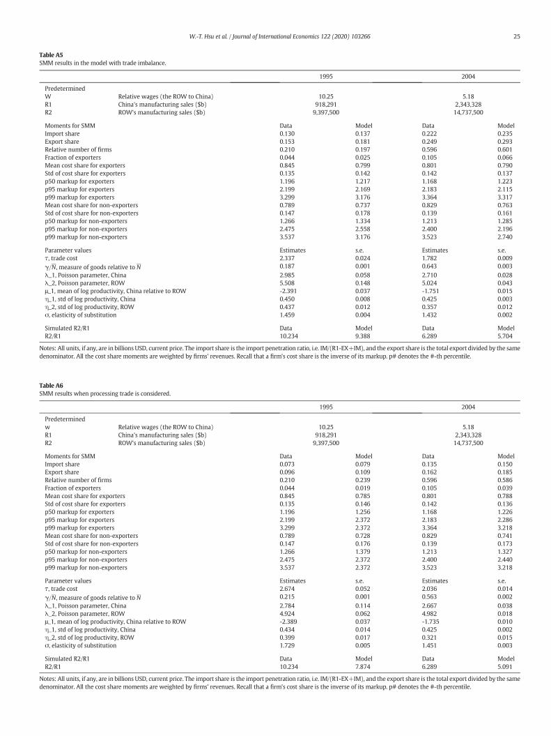
Table A5SMM results in the model with trade imbalance.

1995 2004

PredeterminedW Relative wages (the ROW to China) 10.25 5.18R1 China's manufacturing sales ($b) 918,291 2,343,328R2 ROW's manufacturing sales ($b) 9,397,500 14,737,500

Moments for SMM Data Model Data ModelImport share 0.130 0.137 0.222 0.235Export share 0.153 0.181 0.249 0.293Relative number of firms 0.210 0.197 0.596 0.601Fraction of exporters 0.044 0.025 0.105 0.066Mean cost share for exporters 0.845 0.799 0.801 0.790Std of cost share for exporters 0.135 0.142 0.142 0.137p50 markup for exporters 1.196 1.217 1.168 1.223p95 markup for exporters 2.199 2.169 2.183 2.115p99 markup for exporters 3.299 3.176 3.364 3.317Mean cost share for non-exporters 0.789 0.737 0.829 0.763Std of cost share for non-exporters 0.147 0.178 0.139 0.161p50 markup for non-exporters 1.266 1.334 1.213 1.285p95 markup for non-exporters 2.475 2.558 2.400 2.196p99 markup for non-exporters 3.537 3.176 3.523 2.740

Parameter values Estimates s.e. Estimates s.e.τ, trade cost 2.337 0.024 1.782 0.009γ=N, measure of goods relative to N 0.187 0.001 0.643 0.003λ_1, Poisson parameter, China 2.985 0.058 2.710 0.028λ_2, Poisson parameter, ROW 5.508 0.148 5.024 0.043μ_1, mean of log productivity, China relative to ROW -2.391 0.037 -1.751 0.015η_1, std of log productivity, China 0.450 0.008 0.425 0.003η_2, std of log productivity, ROW 0.437 0.012 0.357 0.012σ, elasticity of substitution 1.459 0.004 1.432 0.002


Notes: All units, if any, are in billions USD, current price. The import share is the import penetration ratio, i.e. IM/(R1-EX+IM), and the export share is the total export divided by the samedenominator. All the cost share moments are weighted by firms' revenues. Recall that a firm's cost share is the inverse of its markup. p# denotes the #-th percentile.

Table A6SMM results when processing trade is considered.

1995 2004

Predeterminedw Relative wages (the ROW to China) 10.25 5.18R1 China's manufacturing sales ($b) 918,291 2,343,328R2 ROW's manufacturing sales ($b) 9,397,500 14,737,500

Moments for SMM Data Model Data ModelImport share 0.073 0.079 0.135 0.150Export share 0.096 0.109 0.162 0.185Relative number of firms 0.210 0.239 0.596 0.586Fraction of exporters 0.044 0.019 0.105 0.039Mean cost share for exporters 0.845 0.785 0.801 0.788Std of cost share for exporters 0.135 0.146 0.142 0.136p50 markup for exporters 1.196 1.256 1.168 1.226p95 markup for exporters 2.199 2.372 2.183 2.286p99 markup for exporters 3.299 2.372 3.364 3.218Mean cost share for non-exporters 0.789 0.728 0.829 0.741Std of cost share for non-exporters 0.147 0.176 0.139 0.173p50 markup for non-exporters 1.266 1.379 1.213 1.327p95 markup for non-exporters 2.475 2.372 2.400 2.440p99 markup for non-exporters 3.537 2.372 3.523 3.218

Parameter values Estimates s.e. Estimates s.e.τ, trade cost 2.674 0.052 2.036 0.014γ=N, measure of goods relative to N 0.215 0.001 0.563 0.002λ_1, Poisson parameter, China 2.784 0.114 2.667 0.038λ_2, Poisson parameter, ROW 4.924 0.062 4.982 0.018μ_1, mean of log productivity, China relative to ROW -2.389 0.037 -1.735 0.010η_1, std of log productivity, China 0.434 0.014 0.425 0.002η_2, std of log productivity, ROW 0.399 0.017 0.321 0.015σ, elasticity of substitution 1.729 0.005 1.451 0.003


Notes: All units, if any, are in billions USD, current price. The import share is the import penetration ratio, i.e. IM/(R1-EX+IM), and the export share is the total export divided by the samedenominator. All the cost share moments are weighted by firms' revenues. Recall that a firm's cost share is the inverse of its markup. p# denotes the #-th percentile.



Next, we calculate

Msell2 wð Þ

¼ R1 wð Þ−DR2 wð Þ

Zω:χ�


1ωϕ1ωdω þ R2 wð Þ þ DR2 wð Þ

Zω:χ�


2ωϕ2ωdω

!−1

;

Finally, given L2, we can use themarket clearing condition of country2 to solve for w:

Msell2 wð Þ ¼ R2 wð Þ

wL2:

Given the solution ofw, equilibrium R1 and R2 can be obtained usingthe above procedure. The SMM result of the modified model is pre-sented in Table A5.

A.7. SMM Results Considering Processing Trade

When considering processing trade, the only changes from thebenchmark SMM procedure are the import and export shares. Fromthe custom data, we first obtain the fraction of processing-trade importin total import. We then use the formula for import and export shares,as well as R1 given in Table 2, to re-calculate export and import shares.The new numbers for 1995 are 0.073 and 0.096 for import and exportshares, respectively. The corresponding numbers for 2004 are 0.135and 0.162. The SMM results are given in Table A6.

References

Ackerberg, D., Caves, K., Frazer, G., 2006. Structural identification of production functions.Working Paper. UCLA.

Ackerberg, D., Benkard, C.L., Berry, S., Pakes, A., 2007. Econometric tools for analyzingmarket outcomes. In: Heckman, James J., Leamer, Edward E. (Eds.), Handbook ofEconometrics. 6A. Elsevier, North-Holland, Amsterdam and Boston, pp. 4171–4276.

Adda, J., Cooper, R.W., 2003. Dynamic Economics: Quantitative Methods and Applications.MIT Press.

Alvarez, Fernando, Lucas, Robert Jr., 2007. General equilibrium analysis of the Eaton-Kortum model of international trade. J. Monetary Econ. 54 (6), 1726–1768.

Arkolakis, C., Costinot, A., Rodríguez-Clare, A., 2012. New trade models, same old gains?Am. Econ. Rev. 102 (1), 94–130.

Arkolakis, C., Costinot, A., Donaldson, D., Rodríguez-Clare, A., 2019. The elusive pro-com-petitive effects of trade. Rev. Econ. Stud. 86 (1), 46–80.

Asturias, Jose, García-Santana, Manuel, Ramos, Roberto, 2017. Competition and the wel-fare gains from transportation infrastructure: evidence from the golden quadrilateralof India. Working Paper. Georgetown University, Qatar.

Atkeson, A., Burstein, A., 2008. Pricing to market, trade costs, and international relativeprices. Am. Econ. Rev. 98 (5), 1998–2031.

Behrens, K., Murata, Y., 2012. Trade, competition, and efficiency. J. Int. Econ. 87 (1), 1–17.Bernard, A.B., Eaton, J., Jensen, J.B., Kortum, S., 2003. Plants and productivity in interna-

tional trade. Am. Econ. Rev. 93 (4), 1268–1290.Brandt, L., Van Biesebroeck, J., Zhang, Y., 2012. Creative accounting or creative destruc-

tion: firm level productivity growth in Chinese manufacturing. J. Dev. Econ. 97 (2),339–351.

Brandt, L., Van Biesebroeck, J., Wang, L., Zhang, Y., 2017. WTO accession and performanceof Chinese manufacturing firms. Am. Econ. Rev. 107 (9), 2784–2820.

Caliendo, L., Parro, F., 2015. Estimates of the trade andwelfare effects of NAFTA. Rev. Econ.Stud. 82 (1), 1–44.

Costinot, A., Rodríguez-Clare, A., 2014. Trade theory with numbers: Quantifying the con-sequences of globalization. Handbook of International Economics. Vol. 4. Elsevier,pp. 197–261.

de Blas, B., Russ, K., 2015. Understanding markups in the open economy under Bertrandcompetition. Am. Econ. J. Macroecon. 7 (2), 157–180.

De Loecker, J., Warzynski, F., 2012. Markups and firm-level export status. Am. Econ. Rev.102 (6), 2437–2471.

De Loecker, J., Goldberg, P.K., Khandelwal, A.K., Pavcnik, N., 2016. Prices, markups andtrade reform. Econometrica 84 (2), 445–510.

Devereux, M.B., Lee, K.M., 2001. Dynamic gains from international trade with imperfectcompetition and market power. Rev. Dev. Econ. 5 (2), 239–255.

Dhingra, S., Morrow, J., 2016. Monopolistic competition and optimum product diversityunder firm heterogeneity. Working Paper. London School of Economics.

di Giovanni, J., Levchenko, A.A., Zhang, J., 2014. The global welfare impact of China: Tradeintegration and technological change. Am. Econ. J. Macroecon. 6 (3), 153–183.

Dixit, A.K., Stiglitz, J.E., 1977. Monopolistic competition and optimum product diversity.Am. Econ. Rev. 67 (3), 297–308.

Eaton, J., Kortum, S., 2002. Technology, geography, and trade. Econometrica 70 (5),1741–1779.

Eaton, J., Kortum, S., Sotelo, S., 2013. International trade: Linking micro and macro. Ad-vances in Economics and Econometrics, 1st ed Vol 2. Cambridge University Press,pp. 329–370.

Edmond, C., Midrigan, V., Xu, D.Y., 2015. Competition, markups, and the gains from inter-national trade. Am. Econ. Rev. 105 (10), 3183–3221.

Epifani, P., Gancia, G., 2011. Trade, markup heterogeneity and misallocations. J. Int. Econ.83 (1), 1–13.

Fajgelbaum, P.D., Khandelwal, A.K., 2016. Measuring the unequal gains from trade. Quart.J. Econ. 131 (3), 1113–1180.

Feenstra, R.C., Weinstein, D.E., 2017. Globalization, markups, and US welfare. Journal ofPolitical Economy 125 (4), 1040–1074.

Feenstra, R.C., 2018. “Restoring the Product Variety and Pro-competitive Gains from Tradewith Heterogeneous Firms and Bounded Productivity”. Journal of International Eco-nomics 110, 16–27.

Head, K., Mayer, T., Thoenig, M., 2014. Welfare and trade without pareto. Am. Econ. Rev.(Papers and Proc.) 104 (5), 310–316.

Helpman, E., Melitz, M., Rubinstein, Y., 2008. Estimating trade flows: Trading partners andtrading volumes. Quart. J. Econ. 123, 441–487.

Holmes, T.J., Hsu, W.-T., Lee, S., 2014. Allocative efficiency, mark-ups, and the welfaregains from trade. J. Int. Econ. 94 (2), 195–206.

Hsieh, C.-T., Klenow, P.J., 2009. Misallocation and manufacturing TFP in China and India.Quart. J. Econ. 124 (4), 1403–1448.

Hsieh, C.T., Ossa, R., 2016. A global view of productivity growth in China. J. Int. Econ. 102,209–224.

Karabarbounis, L., Neiman, B., 2014. The global decline of the labor share. Quart. J. Econ.129 (1), 61–103.

Krugman, P.R., 1979. Increasing returns, monopolistic competition, and internationaltrade. J. Int. Econ. 9 (4), 469–479.

Levinsohn, J.A., Petrin, A.K., 2003. Estimating production functions using inputs to controlfor unobservables. Rev. Econ. Stud. 70 (2), 317–342.

Lipsey, R.G., Lancaster, Kelvin, 1956-1957. The general theory of second best. Rev. Econ.Stud. 24 (1), 11–32.

Lu, Y., Yu, L., 2015. Trade liberalization and markup dispersion: Evidence from China’sWTO accession. Am. Econ. J. Appl. Econ. 7 (4), 221–253.

Markusen, J., 1981. Trade and the gains from trade with imperfect competition. J. Int.Econ. 11, 531–551.

Melitz, M.J., 2003. The impact of trade on intra-industry reallocations and aggregate in-dustry productivity. Econometrica 71 (6), 1695–1725.

Melitz, M.J., Ottaviano, G., 2008. Market size, trade, and productivity. Rev. Econ. Stud. 75(1), 295–316.

Melitz, M.J., Redding, S.J., 2015. New trade models, new welfare implications. Am. Econ.Rev. 105 (3), 1105–1146.

Olley, G.S., Pakes, A., 1996. The dynamics of productivity in the telecommunicationsequipment industry. Econometrica 64, 1263–1298.

Ottaviano, G., Tabuchi, T., Thisse, J.-F., 2002. Agglomeration and trade revisited. Int. Econ.Rev. 43 (2), 409–435.

Restuccia, D., Rogerson, R., 2008. Policy distortions and aggregate productivity with het-erogeneous plants. Rev. Econ. Dyn. 11, 707–720.

Robinson, Joan, 1934. The economics of imperfect competition. Macmillan.Salvo, A., 2010. Inferringmarket power under the threat of entry: The case of the Brazilian

cement industry. RAND J. Econ. 41 (2), 326–350.Schmitz, Jr J.A., 2005. What determines productivity? Lessons from the dramatic recovery

of the U.S. and Canadian iron ore industries following their early 1980s crisis. J. Polit.Econ. 113 (3), 582–625.

Simonovska, I., Waugh, M.E., 2014. Trade models, trade elasticities, and the gains fromtrade. NBER Working Paper w20495.

Trefler, D., 2004. The long and short of the Canada-U.S. free trade agreement. Am. Econ.Rev. 94 (4), 870–895.

Weinberger, A., 2015. Markups and misallocation with trade and heterogeneous firms.Globalization and Monetary Policy Institute Working Paper No. 251. Federal ReserveBank of Dallas.

Zhelobodko, E., Kokovin, S., Parenti, M., Thisse, J.F., 2012. Monopolistic competition:Beyond the constant elasticity of substitution. Econometrica 80 (6), 2765–2784.

http://refhub.elsevier.com/S0022-1996(19)30088-1/rf0005














































































































Competition, markups, and gains from trade: A quantitative ...

Documents

Transcript of Competition, markups, and gains from trade: A quantitative ...