Kiyomi et al. BMC Res Notes (2016) 9:115 DOI 10.1186/s13104-016-1912-y

RESEARCH ARTICLE

Comparison of intra-individual coefficients of variation on the paired sampling data when inter-individual variations are different between measuresFumiaki Kiyomi1*, Masako Nishikawa2, Yoichiro Yoshida3 and Keita Noda4

Abstract

Background: Pain intensities of patients are repeatedly measured by Visual Analog Scale (VAS) and Pain Vision (PV) in a clinical research. Two measurements by VAS and PV are performed at the same time. In order to evaluate within patient consistency, intra-individual coefficient of variations (CVs) are compared between measures assuming that the pain status of each patient is stable during the research period. The correlated samples and different inter-individual variation due to different scales of the measures should be taken into account in statistical analysis. The adjustment of covariates will improve the estimation of population mean values of the measures.

Methods: In this paper, statistical approach to compare the intra-individual CVs is proposed. The approach consists of two steps: (1) estimating population mean values and intra-individual variances of the pain intensities by measure in a mixed effect model framework, (2) computing intra-individual CVs and comparing them between measures. The mixed effect model includes measure and some variables as fixed effects and subject by measure as a random effect. The different inter-individual variations between measures and their covariance reflect the paired sampling in the vari-ance component. The confidence interval of the difference of intra-individual CVs is constructed using the asymptotic normality and the delta method. Bootstrap method is available if sample size is small.

Results: The proposed approach is illustrated using pain research data. Measure (VAS and PV), age and sex are included in the model as fixed effects. The confidence intervals of the difference of intra-individual CVs between measures are estimated by the asymptotic theory and by bootstrap using a subgroup resampling, respectively. Both confidence intervals are similar.

Conclusion: The proposed approach is useful to compare two intra-individual CVs taking it into account to reflect the paired sampling, different inter-individual variations between measures and some covariates. Although the inclu-sion of covariates did not improve the goodness-of-fit in the illustration, the proposed model with covariates will improve the accuracy and/or precision if covariates truly influence response variable. This approach can be applicable with small modification to various situations.

Keywords: Intra-individual variation, Inter-individual variation, Coefficient of variation, Mixed effect model, Paired sampling, Bootstrap

© 2016 Kiyomi et al. This article is distributed under the terms of the Creative Commons Attribution 4.0 International License (http://creativecommons.org/licenses/by/4.0/), which permits unrestricted use, distribution, and reproduction in any medium, provided you give appropriate credit to the original author(s) and the source, provide a link to the Creative Commons license, and indicate if changes were made. The Creative Commons Public Domain Dedication waiver (http://creativecommons.org/publicdomain/zero/1.0/) applies to the data made available in this article, unless otherwise stated.

Open Access

BMC Research Notes

*Correspondence: fumkiyomi@adm.fukuoka-u.ac.jp 1 Academia, Industry and Government Collaborative Research Institute of Translational Medicine for Life Innovation, Fukuoka University, 7-45-1 Nanakuma Jyonan-ku, Fukuoka 814-0180, JapanFull list of author information is available at the end of the article

Page 2 of 8Kiyomi et al. BMC Res Notes (2016) 9:115

BackgroundA clinical research of oxaliplatin chemotherapy was con-ducted in colorectal cancer patients. Pain intensities of oxaliplatin-induced peripheral neuropathy were assessed by two measures of Visual Analog Scale (VAS) and Pain Vision PS-2100 (PV). The two pain assessments were per-formed at the same time on the same set of patients and the assessments were repeated during some time inter-val. VAS is a widely used subjective scale to measure the pain intensity, and patients assess their pain intensities along a continuous line from 0 to 100. PV is an analyti-cal instrument that is designed to assess sense perception and nociception quantitatively and objectively. The pain intensity by PV is defined as a percentage change of two electrical stimulation values with and without pain. Thus measurements by PV are non-negative values (range of the actual data was 0 to about 400). The objective of the research was to compare these subjective and objective measures, and the intra-individual variation was com-pared in order to evaluate the within patient consistency as the reliability index assuming that the pain status of each patient has been stable during the research period. Since the scales of two measures are different, the intra-individual coefficient of variation (CV) is used as a varia-tion index.

In this situation, there are two conditions to be consid-ered in the statistical analysis:

• correlated samples by paired sampling (assessments by VAS and PV were performed at the same time)

• different inter-individual variation between measures (different scales: 0–100 for VAS and non-negative values of 0 to about 400 for PV)

Furthermore, there exists an additional requirement to improve the estimation of population mean values of measures:

• taking covariates into account, for example sex and/or age

In many clinical studies, the standard deviation, the coefficient of variation or a composite index such as the mean amplitude of glycemic excursion (MAGE) in dia-betic area are used as intra-individual variation indexes, and those indexes are calculated for each subject and sometimes compared between groups or treatments by two sample t test, linear regression analysis or analysis of variance [e.g. 1–3]. Onishi et al. [4] compared the intra-individual CVs in pre-breakfast self-measured plasma glucose between treatments including some variables as covariates and subject as a random effect. There are many statistical discussions (e.g. 5, 6) relating to comparing

intra-individual CVs. Forkman [5] gave a method to com-pare intra-individual CVs (although “intra-individual” is not explicitly written). Iron [6] compared several meth-ods to calculate intra-class correlation coefficient (ICC). For the paired sampling, Shoukri et  al. [7] gave several procedures for testing the equality of two dependent intra-individual CVs. They used a mixed model including one fixed effect and subject as a random effect and they gave a covariance structure reflecting the paired sampling to the model. Their procedures, however, did not clearly model the different inter-individual variation and covari-ates were not included either. Furthermore, they assumed that the number of repetition of both measurements was the same for all subjects.

In this article, we propose an approach to compare two intra-individual CVs considering the two conditions (cor-related samples by paired sampling and different inter-individual variation between measures) and adjustment of the covariates. A mixed effect model will be used to estimate population mean values and intra-individual variances for measures. The mixed effect model includes measure and some variables as fixed effects and subject by measure as a random effect. Different inter-individual variation between measures and the paired sampling are taken into account in this model. The number of repeti-tions may be varied among subjects due to missing. By using iterative algorithms in the mixed effect models, we obtain the estimates without restriction of the same number of repetitions. The intra-individual CVs will be calculated and compared using these estimates.

MethodsStatistical modelLet yijk ≥ 0 denote the kth observation of the jth subject by the ith measure, i = 1, 2, j = 1, 2, . . . , n, k = 1, 2, . . . ,mij . Let mj and m be mj = m1j +m2j and m =

∑i,j mij. The

repeated measurements for the jth subject consist of m1j times examinations by the first measure and m2j times examinations by the second measure. If there are missing values, m1j may be different from m2j. Thus, missing val-ues are allowed in the model. In our mixed effect model, yijk is expressed by

where xijk is a p× 1 design vector for fixed effects, β =

(β1, . . . ,βp

)′ is a p× 1 parameter vector of the fixed

effects regression coefficients, γij is the random effect of the jth subject for the ith measure and assumed to be normally distributed γij ∼ N

(0, σ 2

bi

), γ1j and γ2j are corre-

lated by a covariance σ 2b12 and γij and γi′j′ are assumed to

be independent if j �= j′ for i, i′ = 1, 2, eijk is the residual

(1)yijk = x′

ijkβ + γij + eijk ,

Page 3 of 8Kiyomi et al. BMC Res Notes (2016) 9:115

error and is assumed that eijk ∼ i.i.d.N(0, σ 2

ei

). The fixed

effect part x′

ijkβ includes a factor of the measure, where β1 and β2 denote means for the first measure and for the second measure, respectively.

Using notations of vector, the observations of the jth subject and all observations can be expressed by yj and

y, where yj =(y1j1, . . . , y1jm1j , y2jm1j+1, . . . , y2jm1j+m2j

)′

and y =(y′

1, y′

2, . . . , y′

n

)′

, respectively. Let Rj denote a

mj ×mj diagonal matrix for the residuals of the jth sub-ject. It can be seen that

Define R as block diag(R1, . . . ,Rn). The covariance matrix for the random effect of the jth subject can be expressed by g, where

Note that g is the same structure for all j. Define the 2n× 2n matrix G as G = block diag (g , . . . , g). In the matrix notation, the model (1) can be represented by

where X and Z are m× p and m× 2n design matrices for the fixed effects and the random effect of subjects, respectively, γ is a 2n× 1 parameter vector for the ran-dom effect and γ ∼ N (0,G), e is a m× 1 vector of the random residual error and it follows a N (0,R), e and γ are independent. β is the p× 1 parameter vector mentioned above. We can make X full rank. Z consists of m× 1 column vectors of Z1j and Z2j, j = 1, 2, . . . , n, where Zij , i = 1 2, has 1 for the corresponding elements to the jth subject by the ith measure and 0 otherwise.

The expectation and the variance of y are expressed by

The components of V are explained in “Appendix 1”.

Parameter estimation based on likelihoodThe parameters in the model (2) are estimated based on the usual maximum likelihood (ML) approach for linear mixed models. The covariance matrix is estimated by the method of restricted maximum likelihood (REML) where degrees of freedom is adjusted in estimating fixed effects [8–11].

According to [11], the log-likelihood can be partitioned into two parts, L1 and L2. The L1 is the part including β and L2 not including β. The variance and covariance

Rj = diag

σ 2

e1, . . . , σ2e1� �� �

m1j

, σ 2e2, . . . , σ

2e2� �� �

m2j

.

g =

(σ 2b1 σb12

σb12 σ 2b2

).

(2)y = Xβ + Zγ + e,

(3)E(y) = Xβ ,Var(y) = V = ZGZ′+ R.

parameters are estimated using an iterative algorithm based on L2, and fixed effect parameters β are estimated based on the L1 as

For the detail of the parameter estimation, see “Appendix 2”.

Evaluation of the difference of intra‑individual CVsAs mentioned in statistical model section, β1 and β2 represent means of the first and second meas-ure, respectively. Let g

(a) denote the difference of

CVs between measures, where a =(β1, β2, σ

2e1, σ

2e2

)′

, g(a)=

√σ 2e1/β1 −

√σ 2e2/β2. Our objective is to

test H0: g(a) = 0. Using the delta method [12] and E(∂2L1/∂β∂θl

)= 0, the expectation and variance of g

(a)

are obtained as

Under H0, g(a)/

√Var

[g(a)]

has the unit normal dis-tribution by applying the large sample theory, where Var

[g(a)]

is the estimator of Var[g(a)]

obtained by sub-stituting estimators for all parameters. Alternatively the equality of CVs between measures can be evaluated by an interval estimation of the difference of CVs using the

asymptotic normality of g(a)/

√Var

[g(a)]

.Another method to test H0 is bootstrap method [13]

which is particularly useful if sample size is not sufficiently large to apply the asymptotic theory. A simple bootstrap-ping is the subject resampling method with replacement. Since the data is obtained based on the paired sampling, the resampling is taken place by subject (kind of block or cluster bootstrap, [14]) in order to capture the dependence structure. The resampled number of subjects is equal to the size n of the original data set. The resampling will be straightforward if the numbers of observations by measure

(4)β =(X

′V−1X

)−1X

′V−1y

(5)E[g(a)]

≈

√σ 2e1

β1−

√σ 2e2

β2,

(6)

Var[g(a)]

≈1

4β21σ 2e1

Var(σ 2e1

)+

σ 2e1

β41

Var(β1

)

+1

4β22σ 2e2

Var(σ 2e2

)+

σ 2e2

β42

Var(β2

)

+1

4β1β2

√σ 2e1σ

2e2

Cov(σ 2e1, σ

2e2

)

+

√σ 2e1σ

2e2

β21β22

Cov(β1, β2

).

Page 4 of 8Kiyomi et al. BMC Res Notes (2016) 9:115

are the same across the subjects, namely mij = ri, i = 1, 2 for all j = 1, . . . , n . Otherwise, a subgroup resampling classified by number of observations by measure will be one way to make the resample data set with the same records m as in the original data set if two measures (e.g. VAS and PV) are always observed paired although the number of observations may be different among sub-jects. For example, let n1 , n2 and n3 (n1 + n2 + n3 = n) be defined as the number of subjects repeatedly measured twice, thrice and four times, respectively. Thus there are three subgroups. The resampling is performed in the same size ni with replacement from the ith subgroup (i = 1, 2, 3).

There exist another bootstrap methods such as s para-metric bootstrap. Since the objective of this article, how-ever, is not to discuss the bootstrapping, only the blocked and subgrouped way will be used in the later section.

Application resultOur proposed model was applied to the clinical research data mentioned in the background section. Forty-three patients were treated with oxaliplatin chemotherapy. The pain intensity of oxaliplatin-induced peripheral neurop-athy was assessed by two measures of VAS and PV. All patients with repeated measurements were included in the analysis, and the number of records of the data set was m = 158 (see Additional file  1). Summary statistics of age and sex and those of PAS and PV were shown in Tables 1 and 2, respectively.

A stopping criterion of numerical iterations by the Fisher’s scoring method to estimate parameters was set to 10−6. Sex, age, interaction between measure and sex and interaction between measure and age were included in the mixed model as covariates (fixed effects in full model). To obtain the MLEs of β1 (VAS) and β2 (PV) as least square means (LSMs, [15]), let β3, β4, β5 and β6 be regression parameters for sex (0: female, 1: male), interaction between measure and sex (1: VAS and male, 0: otherwise), age and interaction between measure and age (age in year for VAS and 0 for PV). Let xsex and xage denote the proportion of male and mean age, respectively. The MLEs of β1 and β2 are l ′1β

and l′

2β, where l1 =(1 0 xsex xsex xage xage

)′ and

l2 =(0 1 xsex 0 xage 0

)′ and β is obtained by (4). SEs of

LSMs are estimated as SQRT

(l′

i

(X

′V

−1X)−1

li

). Esti-

mated parameters were shown in Table 2.To obtain variance of g

(a), Cov

(σ 2e1, σ

2e2

) and

Cov(β1, β2

) should be estimated as shown in (6) in addi-

tion to the results in Table  3. Using Fisher’s informa-tion matrix we see that Cov

(σ 2e1, σ

2e2

)= −13.2 and

Cov(β1, β2

)= l

′

1

(X

′V

−1X)−1

l2 = 10.0. The difference

of CVs and its 95 % confidence interval was estimated as −0.96 (−1.59, −0.33) by (5) and (6). Thus the intra-individ-ual variation was significantly smaller in the VAS than PV.

Bootstrapping was also conducted as sensitivity analysis of the asymptotic inference. 1000 data sets with the same size as the original sample were generated with replace-ment by the subgroup method, and the model parameters and the difference of CVs between measures were esti-mated for each data set. A Bootstrap estimate of the dif-ference of intra-individual CVs was obtained as the mean of the 1000 estimates, and a 95 % confidence interval was constructed by mean of the 25th and 26th values and mean of the 975th and 976th values out of the 1000 esti-mates. The bootstrap estimate was −0.90 (−1.50, −0.31), and this estimate was similar as in the asymptotic theory.

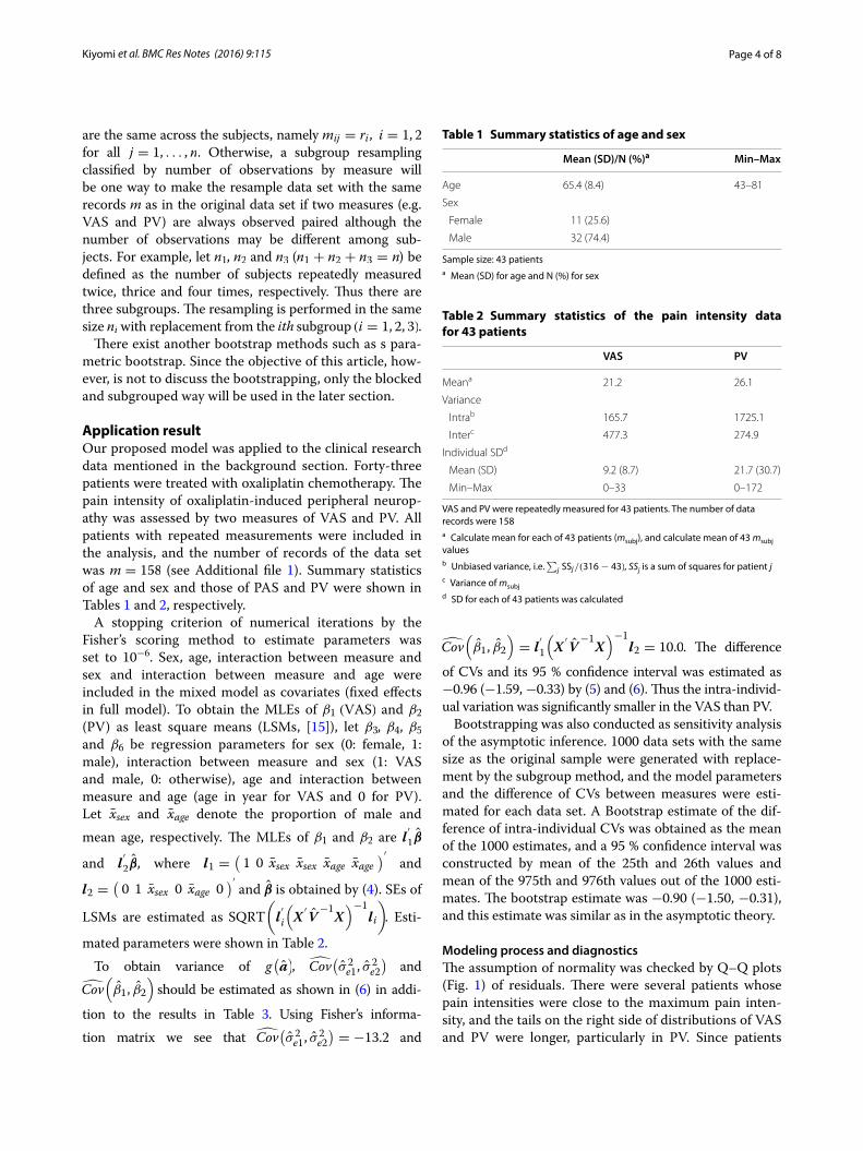
Modeling process and diagnosticsThe assumption of normality was checked by Q–Q plots (Fig.  1) of residuals. There were several patients whose pain intensities were close to the maximum pain inten-sity, and the tails on the right side of distributions of VAS and PV were longer, particularly in PV. Since patients

Table 1 Summary statistics of age and sex

Sample size: 43 patientsa Mean (SD) for age and N (%) for sex

Mean (SD)/N (%)a Min–Max

Age 65.4 (8.4) 43–81

Sex

Female 11 (25.6)

Male 32 (74.4)

Table 2 Summary statistics of  the pain intensity data for 43 patients

VAS and PV were repeatedly measured for 43 patients. The number of data records were 158a Calculate mean for each of 43 patients (msubj), and calculate mean of 43 msubj valuesb Unbiased variance, i.e.

∑j SSj/(316− 43), SSj is a sum of squares for patient j

c Variance of msubjd SD for each of 43 patients was calculated

VAS PV

Meana 21.2 26.1

Variance

Intrab 165.7 1725.1

Interc 477.3 274.9

Individual SDd

Mean (SD) 9.2 (8.7) 21.7 (30.7)

Min–Max 0–33 0–172

Page 5 of 8Kiyomi et al. BMC Res Notes (2016) 9:115

with high pain intensities cannot be excluded from the analysis population for our research objective and a loga-rithmically transformation is not possible for zero values, all patients were included in the statistical analyses. We performed a sensitivity analysis excluding two patients with large values and confirmed similar result as shown in the former analysis.

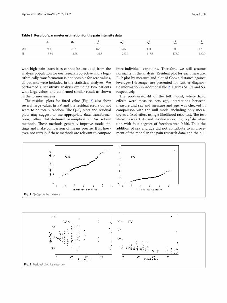
The residual plots for fitted value (Fig.  2) also show several large values in PV and the residual errors do not seem to be totally random. The Q–Q plots and residual plots may suggest to use appropriate data transforma-tions, other distributional assumption and/or robust methods. These methods generally improve model fit-tings and make comparison of means precise. It is, how-ever, not certain if these methods are relevant to compare

intra-individual variations. Therefore, we still assume normality in the analysis. Residual plot for each measure, P–P plot by measure and plot of Cook’s distance against leverage/(1-leverage) are presented for further diagnos-tic information in Additional file 2: Figures S1, S2 and S3, respectively.

The goodness-of-fit of the full model, where fixed effects were measure, sex, age, interactions between measure and sex and measure and age, was checked in comparison with the null model including only meas-ure as a fixed effect using a likelihood ratio test. The test statistics was 3.048 and P-value according to χ2 distribu-tion with four degrees of freedom was 0.550. Thus the addition of sex and age did not contribute to improve-ment of the model in the pain research data, and the null

Table 3 Result of parameter estimation for the pain intensity data

β1 β2 σ 2

e1σ 2

e2σ 2

b1σ 2

b2σ 2

b12

MLE 21.0 26.3 166 1707 474 305 423

SE 3.50 4.25 21.8 220.1 117.6 176.2 120.9

Fig. 1 Q–Q plots by measure

Fig. 2 Residual plots by measure

Page 6 of 8Kiyomi et al. BMC Res Notes (2016) 9:115

model will be applied in practice. Since the objective of this application section is to illustrate the availability of the proposed model, we presented the results of the full model assuming normality.

Summary statistics of individual standard deviations (SDs) in VAS and PV were shown in Table 2. The range of individual SDs were vary from 0 to 33 in VAS and from 0 to 172 in PV. The comparison of the intra-individual CV between VAS and PV corresponds to compare the aver-age individual SDs by mean.

ConclusionStatistical approach to compare two intra-individual CVs considering the paired sampling, different inter-individual variations between measures and some covariates was proposed. The approach is (1) esti-mating intra-individual variances and mean values of measures by the mixed effect model including meas-ure and some covariates as fixed effects and subject by measure as a random effect to reflect different inter-individual variation between measures and the paired sampling, (2) computing intra-individual CVs and comparing these CVs between measures. The utility of the approach was shown by applying to the real pain research data. Although the inclusion of covariates did not improve the goodness-of-fit in the illustration, the proposed model with covariates will improve the accuracy and/or precision if covariates truly influence response variable.

The proposed approach is applicable for many situa-tions. One example is to give σ 2

b1 = σ 2b2 = σ 2

b if the same inter individual variations can be assumed between measures. In a study [16], the frequently-sampled intra-venous glucose tolerance test was carried out for subjects by two protocols in order to estimate insulin sensitivity, and intra-individual CVs of the insulin sensitivity were compared between protocols. If our proposed model is applied to this data, the same inter individual variation (σ 2

b1 = σ 2b2) for two protocols will be observed since the

same scaled variable was measured by the two different protocols.

Another example is to compare intra-individual vari-ances σ 2

ei(z) (i = 1, 2) by analyzing zijk = log(yijk

) if log-

normal distributions can be assumed for yijk and the geometric CV [17] of the original data can be approxi-mated by SQRT

{exp

(σ 2ei(z)

)− 1

}∼= σ 2

ei(z), where σ 2ei(z)

is the residual error variance of zijk and it is assumed to be small enough to hold the approximation. The approximation of the geometric CV means that CVs in original scale data can be approximated by variances in the logarithmically transformed data. This procedure suggests to omit the CV calculation step. For example,

area under the pharmacokinetic curve and triglyceride have such characteristics. These variables have skewed distributions with longer tail upper side, and are fre-quently logarithmically transformed before statistical analyses. However, note that possible biases should be discussed before the transformation since the logarith-mic transformation can give a larger benefit to a group with large values than the other group with small values when estimating population intra-individual variances.

An extension to multi-group comparisons is straight-forward by giving corresponding Rj and Gj and by deriv-ing derivatives of V .

AbbreviationsCV: coefficient of variation; ICC: intra-class correlation coefficient; IRB: insti-tutional review board; LSM: least square mean; MAGE: mean amplitude of glycemic excursion; ML: maximum likelihood; PV: pain vision; REML: restricted maximum likelihood; VAS: visual analog scale.

Authors’ contributionsYY initiated the pain intensity research, prepared the protocol and got approval of the Institutional Review Board (IRB) of Fukuoka University Hospital. KN reviewed the protocol and organized our team. YY and KN gave significant medical inputs. FK developed the main statistical method of this manuscript, analyzed the data and prepared the manuscript. MN deeply reviewed the derivations of equations and gave critical theoretical inputs. All authors read and approved the final manuscript.

Author details1 Academia, Industry and Government Collaborative Research Institute of Translational Medicine for Life Innovation, Fukuoka University, 7-45-1 Nanakuma Jyonan-ku, Fukuoka 814-0180, Japan. 2 Clinical Research Sup-port Center, The Jikei University School of Medicine, 3-25-8 Nishishinbashi Minato-ku, Tokyo 105-8461, Japan. 3 Department of Gastroenterological Surgery, Fukuoka University Faculty of Medicine, 7-45-1 Nanakuma Jyonan-ku, Fukuoka 814-0180, Japan. 4 Clinical Research Assist Center, Fukuoka University Hospital, 7-45-1 Nanakuma Jyonan-ku, Fukuoka 814-0180, Japan.

AcknowledgementsThis research was not part of any funded project. We thank investigators of Department of Gastroenterological Surgery, Fukuoka University Faculty of Medicine for providing data.

Competing interestsThe authors declare that they have no competing interests.

Appendix 1: Components of variance VLet V j = Var

(yj) denote the mj ×mj variance matrix

of the jth subject. Note that V j , j = 1, . . . , n, have the same structure except the dimension of the repetition mij , i = 1, 2. The variance matrix V is given as below.

Additional files

Additional file 1. A list of the pain intensity data.

Additional file 2. Supplemental figures for the pain intensity data (resid-ual plots, P–P plots and Cook’s distance against leverage/(1-leverage)).

V = block diag (V 1, . . . ,V n),

Page 7 of 8Kiyomi et al. BMC Res Notes (2016) 9:115

where

Iu is a u× u unit matrix and Ju×v is a u× v matrix with all the elements equal to 1.

Appendix 2: Parameter estimationAccording to [11], the log-likelihood can be partitioned into two parts, L1 and L2, where L1 is the part including β and L2 not including β. L1 and L2 are expressed as below.

where C is a certain constant and P = V−1 − V−1X

(X

′V−1X

)−X

′V−1.

The variance and covariance parameters θ = (θ1, θ2, θ3, θ4, θ5)

′

=(σ 2e1, σ

2e2, σ

2b1, σ

2b2, σ

2b12

)′ are esti-

mated based on L2, while the fixed effect parameters β are estimated based on the L1. The first order derivatives of L2 is

∂V /∂θl are obtained by simple manipulations as

V j =

(A1j B12j

B′

12j A2j

),

Aij =

σ 2bi + σ 2

ei σ 2bi · · · σ 2

biσ 2bi σ 2

bi + σ 2ei · · · σ 2

bi· · · · · · · · · · · ·

σ 2bi σ 2

bi · · · σ 2bi + σ 2

ei

= σ 2biJmij×mij + σ 2

eiImij

B12j =

σb12 · · · σb12· · · · · · · · ·σb12 · · · σb12

= σb12Jm1j×m2j ,

(7)

L1 = −1

2

[p log 2π + log

∣∣∣(X ′V

−1X)−1

∣∣∣

+{(X

′V

−1X)−1

X′V

−1y − β

}′

(X′V

−1X)

×{(X

′V

−1X)−1

X′V

−1y − β}

],

(8)L2 = −1

2

[C + log |V | + log

∣∣∣X ′V−1X

∣∣∣+ y′Py

],

(9)∂L2

∂θl= −

1

2

[tr

(P∂V

∂θl

)− y

′P∂V

∂θlPy

].

∂V

∂σ 2ei

= diag

(∂R1

∂σ 2ei

, . . . ,∂Rn

∂σ 2ei

),

∂Rj

∂σ 2e1

= diag (1, . . . , 1, 0, . . . , 0),

∂Rj

∂σ 2e2

= diag (0, . . . , 0, 1, . . . , 1)

ML estimates θ are the solution of the estimating equa-tions ∂L2/∂θl = 0. Usually ML estimates θ are not expressed explicitly and therefore an iterative algorithm such as Newton–Raphson method is used to obtain θ . Fisher’s scoring method, in which Fisher’s information matrix I (θ) is used instead of Hessian in Newton–Raph-son method, is now employed as the iterative algorithm, since I(θ) is a simpler form than Hessian in mixed mod-els and the asymptotic variance of θ can be estimated by I−1(θ) (not observed information [18]). Thus second order derivatives are needed to apply the algorithm

where θk is the kth estimates, θk+1 is an improved one, 0 < c < 1 is a constant value to adjust an improvement quantity and S(θk) = (∂L2/∂θl)|θ=θk.

Simple manipulations give second order derivatives of L2 and I(θ), where the (θl , θl′) element of the former and the latter as can be expressed as

respectively. With respect to β, the ML estimator is derived as the solution of the first order derivatives of (7) equal to 0 as

(10)

∂V

∂σ 2b1

= Z

1 0

0 0

. . .

1 0

0 0

Z

′,

∂V

∂σ 2b2

= Z

0 0

0 1

. . .

0 0

0 1

Z

′

∂V

∂σb12= Z

0 11 0

. . .

0 11 0

Z

′.

θk+1 = θk + cI−1(θk)S(θk),

∂2L2

∂θl∂θl′= −

1

2

[tr

(−P

∂V

∂θl′P∂V

∂θl

)+ y

′P∂V

∂θl′P∂V

∂θlPy

+y′P∂V

∂θlP∂V

∂θl′Py

],

(11)

E

(−

∂2L2

∂θl∂θl′

)=

1

2tr

(−P

∂V

∂θl′P∂V

∂θl

), l, l

′= 1, 2, . . . , 5,

(12)β =(X

′V−1X

)−1X

′V−1y

Page 8 of 8Kiyomi et al. BMC Res Notes (2016) 9:115

• We accept pre-submission inquiries

• Our selector tool helps you to find the most relevant journal

• We provide round the clock customer support

• Convenient online submission

• Thorough peer review

• Inclusion in PubMed and all major indexing services

• Maximum visibility for your research

Submit your manuscript atwww.biomedcentral.com/submit

Submit your next manuscript to BioMed Central and we will help you at every step:

β is actually estimated by substituting V for V in (13) as

β =(X

′V

−1X)−1

X′V

−1y. To obtain the variance of β

and covariance of β and θ, the second order derivatives of (7) are substituted. These are actually the asymptotic variance of β and covariance of β and θ:

Note that in taking expectation of (14), we obtain E(∂2L1/∂β∂θl

)= 0 and hence all covariances of βl and

θl′ are 0 [19].

Received: 16 September 2015 Accepted: 3 February 2016

References 1. Belle J, Raalten T, Bos D, Zandbelt B, Oranje B, Durston S. Capturing the

dynamics of response variability in the brain in ADHD. NeuroImage: Clin. 2015;7:132–41.

2. Jin Y, Su X, Yin G, Xu X, Lou J, Chen J, Zhou Y, Lan Y, Jiang B, Li Z, Lee K, Ye L, Ma J. Blood glucose fluctuations in hemodialysis patients with end stage diabetic nephropathy. J Diabetes Complications. 2015;29:395–9.

3. Bohm M, Schumacher H, Leong D, Mancia G, Unger T, Schmieder R, Cus-todis F, Diener H, Laufs U, Lonn E, Sliwa K, Teo K, Fagard R, Redon J, Sleight P, Anderson C, Donnell M, Yusuf S. Cognitive decline and blood pressure. Hypertension. 2015;65:651–61.

(13)∂2L1

∂β∂β′ = −X

′V−1X ,

(14)∂2L1

∂β∂θl= −X

′V−1 ∂V

∂θlV−1(y − Xβ).

4. Onishi Y, Iwamoto Y, Yoo SJ, Clauson P, Tamer SC, Park S. Insulin degludec compared with insulin glargine in insulin-na€ıve patients with type 2 diabetes: a 26-week, randomized, controlled, Pan-Asian, treat-to-target trial. J Diabetes Investig. 2013;4:605–12.

5. Forkman J. Estimator and tests for common coefficients of variation in normal distributions. Commun Stat Theory Methods. 2008;38:233–51.

6. Ionan AC, Polley MC, McShane LM, Dobbin KK. Comparison of confidence interval methods for an intra-class correlation coefficient (ICC). BMC Med Res Methodol. 2014. doi:10.1186/1471-2288-14-121.

7. Shoukri MM, Colak D, Kaya N, Donner A. Comparison of two depend-ent within subject coefficients of variation to evaluate the repro-ducibility of measurement devices. BMC Med Res Methodol. 2008. doi:10.1186/1471-2288-8-24.

8. Patterson HD, Thompson R. Recovery of interblock information when block sizes are unequal. Biometrika. 1971;31:100–9.

9. Harville DA. Bayesian inference for variance components using only error contrasts. Biometrika. 1974;61:383–5.

10. Harville DA. Maximum likelihood approaches to variance component entimation and to related problems. J Am Stat Assoc. 1977;72:320–40.

11. Verbyla AP. A conditional derivation of residual maximum likelihood. Aust J Stat. 1990;32:227–30.

12. Rao CR. Linear statistical inference and its applications. 2nd ed. New York: Wiley; 1973.

13. Efron B, Tibshirani RJ. An introduction to the bootstrap. 1st ed. New York: Chapman and Hall; 1993.

14. Lahiri SN. Resampling methods for dependent data. 1st ed. New York: Springer; 2003.

15. SAS/STAT(R) 9.3 User’s Guide. Lsmeans statement, the mixed procedure. http://www.biomedcentral.com/bmcmedresmethodol/authors/instruc-tions/researcharticle#formatting-references. Accessed 29 July 2015.

16. Borai A, Livingstone C, Shafi S, Zarif H, Ferns G. Insulin sensitivity (Si) assessment in lean and overweight subjects using two different proto-cols and updated software. Scand J Clin Lab Invest. 2010;70:98–103.

17. Kirkwood TBL. Geometric means and measures of dispersion. Biometrics. 1979;35:908–9.

18. Schervish MJ. Theory of statistics. 1st ed. New York: Springer; 1995. 19. Searle RS, Casella G, McCulloch CE. Variance Components. London: Wiley

Interscience; 1992.