i

Comparison of Creep Compliance Master Curve Models for Hot Mix Asphalt

Myunggoo Jeong

Thesis submitted to the faculty of the Virginia

Polytechnic Institute and State University in partial fulfillment of the requirements for the

degree of

Master of Science

In

Civil and Environmental Engineering

Dr. Gerardo Flintsch, Co-Chair Dr. Amara Loulizi, Co-Chair

Dr. Antonio Trani

July, 2005

Blacksburg, Virginia

Keyword: Viscoelasticity, Creep Compliance, Interconversion, Hot Mix Asphalt

ii

Comparison of Creep Compliance Master Curve Models for Hot Mix Asphalt

Myunggoo Jeong

Abstract

The creep compliance of Hot Mix Asphalt (HMA) is an important property in

characterizing the material’s viscoelastic behavior. It is used to predict HMA thermal

cracking at low temperature and permanent deformation at high temperatures. There

are several experimental methods to measure the creep compliance. Two of these

methods were used in this thesis: the uniaxial compressive and indirect tension (IDT)

creep compliance. The tests were conducted at five temperatures (-15, 5, 20, 30, and

40°C) with a static loading for 1000-sec to characterize two typical HMA mixes used in

Virginia, a base and a surface mix. Creep compliance master curves (CCMC) were

developed by shifting the curves to a reference temperature using time-temperature

superposition. Three mathematical functions, the Prony series, power and sigmoidal,

were fitted to the experimental data using regression analysis. Uniaxial CCMC were

also predicted based on dynamic modulus measurements using method for

interconversion of vicoelastic properties recommended in the literature. Finally, the

susceptibility of the mixes to thermal cracking was evaluated based on the creep

compliance measurements at low temperature.

The regression analysis showed that the three mathematical models considered are

appropriate to model CCMC over a wide range of reduced times. The sigmoidal model

provided the best fit over the entire range of reduced times investigated. This model

also produced the best results when used in the interconversion procedures. However,

there were noticeable differences between the CCMC predicted using interconversion

and the experimental measurements, probably due to nonlinearity in the material

behavior. The m-values for the base mix were higher than those for the surface mix

using the creep results measured with both configurations.

iii

Acknowledgements

I would like to express my utmost appreciation to my advisor, Dr. Flintsch for his time,

patience and advice. He has provided me with several opportunities to do research. I

could not have done this thesis without his support. I also would like to thank Dr. Loulizi,

who has always advised me as a co-chair, mentor and friend. He took the time to listen

to me and advised me whenever I faced unexpected problems. I would like to extend my

gratitude also to my thesis committee, Dr. Trani for his valuable comments and

suggestions.

I would also like to thank my colleagues at the Virginia Tech Transportation Institute: I

express my gratitude to Billy and Samer in the asphalt lab, who helped me prepare lab-

tests and answered a number of questions I asked. I am also grateful to Aris, Carlos,

Chen Chen, Edgar, Hao, Jae, Sangjun and Zheng.

I owe many thanks to my fiancé, Kyung-A, for her unending love and understanding. She

will hold a special place in my heart until the end of my life.

Finally, I am grateful to my brothers, Wan Goo and Bong Goo for their support and care

throughout my life, and to my beloved mother, Choon Ae Kim who is the meaning of my

life and the reason I breathe. I appreciate her sacrifice, endurance and endless love.

iv

TABLE OF CONTENTS

Chapter 1 Introduction................................................................................................1 1.1. Background .......................................................................................................1 1.2. Problem Statement............................................................................................2 1.3. Objectives..........................................................................................................2 1.4. Significance .......................................................................................................3 1.5. Research Scope................................................................................................3

Chapter 2 Literature Review.......................................................................................4 2.1. Introduction........................................................................................................4 2.2. The Creep Compliance .....................................................................................4

2.2.1. Creep Compliance Test Configurations.....................................................6 2.2.2. Creep Compliance Models ........................................................................8

2.3. The Relaxation Modulus..................................................................................10 2.4. Time-Temperature Superposition and Master Curve ......................................12 2.5. Dynamic (Complex) Modulus ..........................................................................14 2.6. Sigmoidal Functions for Modeling Mater Curves.............................................17 2.7. Interconversion among Viscoelastic Material Properties.................................18

2.7.1. Interconversion between the Relaxation Modulus and Creep

Compliance…..........................................................................................................18 2.7.2. Interconversion between the Relaxation Modulus / Creep Compliance and

Dynamic Modulus....................................................................................................20 2.8. Thermal Cracking Models ...............................................................................21

2.8.1. Empirical-based Models for Thermal Cracking on Flexible Pavement ....22 2.8.2. Mechanistic-based Models ......................................................................23 2.8.3. M-E Design Guide Model (2002) .............................................................24

Chapter 3 Experimental Program.............................................................................27 3.1. Introduction......................................................................................................27 3.2. Sample Preparation and Conditioning.............................................................27 3.3. Test Methods...................................................................................................31

3.3.1. Uniaxial Creep Test .................................................................................31 3.3.2. Indirect Tensile Creep Test .....................................................................32

3.4. Test Results ....................................................................................................33 Chapter 4 Creep Compliance Master Curves ..........................................................37

4.1. Introduction......................................................................................................37

v

4.2. Fitting Creep Compliance Master Curve Models.............................................37 4.2.1. CCMC Construction.................................................................................37 4.2.2. CCMC Mathematical Model Fitting..........................................................40

4.3. Effect of the Thermal Cracking Model using the m-value................................47 4.4. Summary .........................................................................................................50

Chapter 5 Interconversion between the Dynamic Modulus and Creep Compliance 51 5.1. Introduction......................................................................................................51 5.2. Conversion from the Dynamic Modulus to Creep Compliance........................51

5.2.1. Prediction of the Relaxation Modulus from the Dynamic Modulus ..........51 5.2.2. Prediction of the Creep Compliance from the Relaxation Modulus .........54 5.2.3. Comparison of Computed versus Measured Creep Compliances ..........55

5.3. Comparison from the Creep Compliance to the Dynamic Modulus.................57 5.4. Summary .........................................................................................................59

Chapter 6 Findings, Conclusions, and Recommendations ......................................60 6.1. Findings...........................................................................................................60 6.2. Conclusions.....................................................................................................61 6.3. Recommendations ..........................................................................................61

References….. ................................................................................................................63 Appendix A: Fitting model SAS Input and Output ...........................................................66

vi

List of Figures

Figure 2.1 Strain-time response for HMA mixtures for a static creep test.........................5 Figure 2.2 Domains of the creep compliance....................................................................8 Figure 2.3 Regression constants D1 and m ......................................................................9 Figure 2.4 Generalized Maxwell model...........................................................................10 Figure 2.5 Creep compliances measured at different temperatures (Before construction)

................................................................................................................................13 Figure 2.6 The creep compliance master curve (After construction) ..............................13 Figure 2.7 The shift factor versus temperature ...............................................................14 Figure 2.8 Stress and strain during a dynamic modulus test ..........................................15 Figure 2.9 Loss and storage modulus.............................................................................16 Figure 2.10 Estimating fracture temperature (After Hill and Brien, 1966) .......................23 Figure 2.11 Thermal cracking development mechanism ................................................24 Figure 2.12 Schematic of crack depth model (after Hiltunen and Roque, 1995) ............25 Figure 3.1 Sieve analysis for the BM25.0 aggregate ......................................................28 Figure 3.2 Sieve analysis for the SM9.5A aggregate......................................................29 Figure 3.3 Sample conditioning chamber and schematic of set up for a uniaxial creep

test ..........................................................................................................................31 Figure 3.4 Prior-to-mounting (right) and mounted (left) specimens using a fixture device

................................................................................................................................31 Figure 3.5 Schematic of environment and set up for an IDT...........................................32 Figure 3.6 Uniaxial creep compliances for the BM25.0...................................................34 Figure 3.7 Uniaxial creep compliances for the SM9.5A ..................................................35 Figure 3.8 IDT creep compliances for the BM25.0..........................................................35 Figure 3.9 IDT creep compliances for the SM9.5A .........................................................36 Figure 4.1 Relationship between shift factor and testing temperatures ..........................38 Figure 4.2 CCMCs of each mix and testing setup...........................................................39 Figure 4.3 The Prony series fit with increasing the number of terms ..............................41 Figure 4.4 Prony series models for the uniaxial CCMC ..................................................42 Figure 4.5 Prony series models for the IDT CCMC.........................................................42 Figure 4.6 Effect of the sigmoidal function coefficients on the CCMC ............................43 Figure 4.7 Sigmoidal models for the uniaxial CCMC ......................................................44 Figure 4.8 Sigmoidal models for the IDT CCMC.............................................................45

vii

Figure 4.9 Power models for the uniaxial CCMC............................................................46 Figure 4.10 Power models for the IDT CCMC ................................................................47 Figure 4.11 The power model at low temperatures from uniaxial setup .........................48 Figure 4.12 The power model at low temperatures from IDT setup................................48 Figure 4.13 M-values for both mixes obtained from the power models ..........................49 Figure 5.1 Storage modulus and sigmoidal fitting curve (BM25.0) .................................52 Figure 5.2 Predicted relaxation modulus (BM25.0).........................................................52 Figure 5.3 Storage modulus and sigmoidal fitting curve (SM9.5A) .................................53 Figure 5.4 Predicted relaxation modulus (SM9.5A) ........................................................53 Figure 5.5 The relaxation modulus and predicted creep compliance (BM25.0)..............54 Figure 5.6 The relaxation modulus and predicted creep compliance (SM9.5A) .............55 Figure 5.7 Comparison of the creep compliance predicted from the dynamic modulus

and determined in the lab test (BM25.0) .................................................................56 Figure 5.8 Comparison of the creep compliance predicted from the dynamic modulus

and determined in the lab test (SM9.5A).................................................................56 Figure 5.9 The predicted dynamic modulus (BM25.0) ....................................................57 Figure 5.10 The predicted dynamic modulus (SM9.5A)..................................................58 Figure 5.11 Comparison of the predicted and measured dynamic moduli (BM25.0) ......58 Figure 5.12 Comparison of predicted and measured dynamic moduli (SM9.5A)............59

viii

List of Tables

Table 3.1 Mixing percentages and material source of BM 25.0 ......................................28 Table 3.2 Mixing percentages and material source of SM 9.5A......................................28 Table 3.3 Molded and testing specimen sizes ................................................................29 Table 3.4 VTM and Gmb for molded specimens ..............................................................30 Table 3.5 Summary of test specimens for creep analysis...............................................30 Table 3.6 Coefficients used to calculate the creep compliance (Kim at el., 2002)..........33 Table 4.1 Summary of creep compliance shift factors ....................................................38 Table 4.2 Regression results: the Prony series fitting.....................................................41 Table 4.3 Regression results: Sigmoidal function fitting .................................................44 Table 4.4 Regression results: Power function fitting .......................................................46 Table 4.5 Regression results: Power model at low temperatures...................................49

1

Chapter 1 Introduction

1.1. Background

When a pavement system is subjected to traffic and/or environmental loading, the stresses

induced by the loads produce critical strains in various locations within the pavement system.

These critical strains can be used to predict pavement performance. The maximum vertical

compressive strains developed in hot-mix asphalt (HMA) layers are used to predict rutting

failure. The maximum tensile strains developed at the top and bottom of HMA layer are used to

predict thermal and fatigue distresses in the HMA.

Material characterization properties are needed in order to model the pavement and compute

the stresses and strains. Flexible pavements are commonly modeled as multilayer linear elastic

systems. Thus, the relevant properties are the modulus of elasticity and the Poisson’s ratio.

However, HMA (a mixture of asphalt binder and aggregate) behaves as a viscoelastic material

since its response depends on the temperature and time of loading. Thus, it is important to

measure the viscoelastic properties of the material at a wide range of frequencies and

temperatures. One of the most common methods for characterizing the response of viscoelastic

materials to loading is to measure their creep behavior at different temperatures and times. The

various measurements are then shifted using time-temperature superposition to build a creep

compliance master curve (CCMC).

The creep test of HMA is of significance because this test makes it possible to determine and

separate the time-independent (elastic strain) and time-dependent (viscoelastic and plastic

strains) components of the strain response (Witczak et al., 2002). In addition, parameters

obtained from creep tests at low temperatures (m-value) are used to predict thermal cracking

development and propagation, and those at high temperatures are used to predict rutting in the

HMA.

There are two commonly used creep tests: the indirect tensile test (IDT) and the uniaxial

compression/tension test. The direct compressive creep test, usually called the uniaxial creep

2

test, is used to predict permanent deformation (rutting) on the surface of pavement, whereas the

IDT is used to characterize HMA mixtures for thermal cracking prediction at low temperatures.

The two creep configurations, IDT and uniaxial creep test for HMA mixtures, were utilized in this

research. Test temperature ranged from -15 to 40°C. Two mixes were studied: a surface mix

(SM9.5A) and a base mix (BM25.0). These mixtures were part of a Material Characterization

Project conducted at the Virginia Tech Transportation Institute (VTTI) (Flintsch et al., 2005). To

minimize the effects of sample preparation on the comparison, all the samples were compacted

using the same Troxler Gyratory Compactor. Ten samples were prepared for each mix.

1.2. Problem Statement

Two mathematical models have been used to represent CCMC: the Prony series and the power

models. The Prony series was used because it has a mechanical analogy and because this

model is efficient when a Laplace transformation is used to interconvert various viscoelastic

properties. However, finding the most appropriate number of terms and the coefficients of the

series may be a tedious and time-consuming exercise even if a statistical package is employed.

The power model is simpler and has been extensively used to find the m-value, which measures

the mix susceptibility to thermal cracking. However, it can only explain the trend of the creep

compliance over a limited range of reduced times.

1.3. Objectives

The main goal of this investigation was to find the most appropriate mathematical models to

represent the CCMC obtained from measurements using the two creep test configurations. The

two commonly used models (the Prony series and power models) as well as a new model (the

sigmoidal function) were studied. Furthermore, the effect of the m-value resulting from the

power model on thermal cracking prediction was examined and comparisons among

viscoelastic material functions were analyzed using interconversion methods.

3

1.4. Significance

Finding statistical CCMC models and comparing them convey a fundamental understanding of

viscoelastic materials. Additionally, the CCMC mathematical models not only provide a general

understanding of how the creep compliance varies over a broad band of reduced times, but also

help estimate a particular creep value at a given reduced time. Furthermore, if the

interconversion method proves accurate, it can facilitate converting viscoelastic properties such

as the creep compliance, relaxation modulus, and dynamic (complex) modulus.

1.5. Research Scope

To accomplish the objective of this research, specimens were tested using IDT and uniaxial

configurations. Regression and graphical data analyses were employed to model the material

response and compare the results from both tests. Several analytical conversions among

viscoelastic properties were also investigated.

This thesis is comprised of six chapters. Chapter 2 presents the background on the creep

behavior of asphalt materials, covering creep tests, testing setup, and models to characterize

the material. Chapter 3 describes the testing program conducted in the study, including the

preparation and mixing of materials, testing equipment, and test protocols. Chapter 4 presents

the construction of CCMC, the statistical modeling of the CCMC, and their application to predict

thermal cracking at low temperatures. Chapter 5 compares viscoelastic properties predicted

through interconversion methods with those measured directly in the lab. Chapter 6 presents

the findings and conclusions of the research along with recommendations for future research.

4

Chapter 2 Literature Review

2.1. Introduction

This chapter reviews the most relevant published reports and papers on the measurement of

viscoelastic material properties, such as the creep compliance, relaxation modulus, and

dynamic modulus; testing methods to measure these properties; thermal cracking mechanism

and models; and interconversion procedures.

2.2. The Creep Compliance

Creep is defined as a time-dependent deformation that occurs when a material is subjected to

loading over time. The modulus of a material, which is simply the reciprocal of the compliance,

is used to model pavement systems and predict stresses, strains, and distresses (Witczak et al.,

2002). However, when considering the viscoelastic behaviour of asphalt materials, it is often

more advantageous to use the creep compliance than to use the modulus because the

compliance can allow separation of its response over time into time-dependent and time-

independent components (Witczak et al., 2002). In a creep test a static load is applied to a

specimen and the deformation over time is measured. The creep compliance is then computed

using Equation (1).

0

( )( ) tD t εσ

= (1)

where

D(t) = creep compliance,

t = testing time,

( )tε = strain at a given time, and

0σ = constant stress.

5

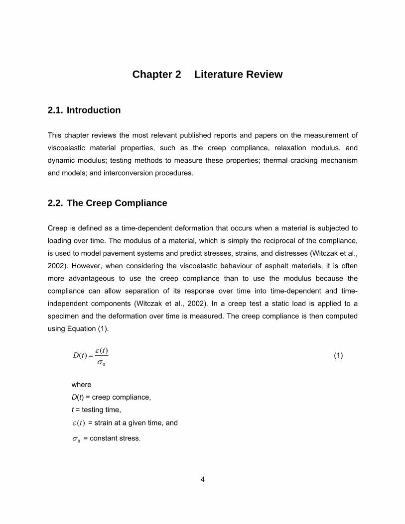
The typical strain versus time response of HMA on a single load-unload cycle is illustrated in

Figure 2.1. This figure shows all the components of the deformation of a viscoelastic material

under a static load. The total strain (εT) can be divided into recoverable and irrecoverable

components, both with time-dependent and time-independent subcomponents as shown in

Equation (2). A material with a high creep compliance at a certain time is prone to deform more

than a material with a relatively low compliance value at the same time.

T e p ve vpε ε ε ε ε= + + + (2)

where

Tε = total strain,

eε = elastic strain (recoverable and time-independent),

eε = plastic strain (irrecoverable and time-independent),

veε = viscoelastic strain (recoverable and time-dependent), and

vpε = viscoplastic strain (irrecoverable and time-dependent).

ε

Tε eε

eε

pε

veεve vpε ε+

p vpε ε+

Figure 2.1 Strain-time response for HMA mixtures for a static creep test

6

2.2.1. Creep Compliance Test Configurations

There are different laboratory testing modes for measuring the creep compliance of HMA:

uniaxial, triaxial, or indirect tensile. The uniaxial configuration has traditionally been used to

characterize and predict permanent deformation of flexible pavement because the data analysis

is simple and the geometry of this test is believed to replicate the asphalt behavior in situ. A

detailed review of the uniaxial test is presented in Chapter 3. The triaxial mode of testing is even

more representative of in-situ conditions because the horizontal confinement is similar to that in

the field. However, the mode is not widely used due to the complexity of setting up the

equipment.

Brown and Foo (1994) compared the unconfined and confined uniaxial (triaxial) creep tests and

their ability to predict rutting in HMA. As expected, it was found that the unconfined uniaxial

creep test was not capable of simulating field conditions because the samples failed when

subjected to high stress and temperature. Conversely, confined creep test mimicked field

conditions fairly well. It was also found that the air void in the samples was reduced after the

unconfined creep test. This is contrasted with phenomenon that occurred in the field. The

researchers recommended the use of confined creep tests for characterizing rutting

performance.

The indirect tensile (IDT) creep test was chosen by the Strategic Highway Research Program

(SHRP) to characterize thermal cracking performance of HMA at low temperatures (Roque et al.

1995). The test is considered the most promising method to predict HMA performance at low

temperatures (Christensen et al. 2004). In particular, this test is used to determine a fracture

property (the m-value) of HMA at low temperatures. The procedure has been standardized in

AASHTO T332 “Standard Method of Test for determining the Creep Compliance and Strength

of Hot-Mix Asphalt (HMA) Using the Indirect Tensile Test Device.”

One advantage of the IDT is that it uses a compressive loading method that is applied to a

cylindrical specimen to create a uniform state of tensile stress in the perpendicular direction

(Roque et al., 1995). It is assumed that the loading alignment is perfect. The indirect tensile

creep test measures the horizontal and vertical displacement next to the center of a cylindrical

specimen. The measurements are then used to compute the Poison ratio and the creep

compliance. The main disadvantage is that the stress and strain distributions are more complex

7

than those of uniaxial test. The mathematical models used to describe the IDT creep

compliance are similar to those used for the uniaxial creep test.

Christensen and Bonaquist (2004) conducted an extensive comparison of HMA creep

compliance measurements using different testing setups: uniaxial tension, uniaxial compression,

and the IDT. The investigation focused on the following issues:

• Evaluation of the difference between creep compliances determined in tension and

compression at low temperatures

• Comparison of the creep compliances measured with in the IDT and uniaxial setups

• Identification of any relationship between the two tests

The creep tests were performed using various types of HMA at three low temperatures (-20, -10,

and 0°C) for 100 seconds. The comparison showed that the creep compliances in tension were

higher than those in compression. The difference increased at higher temperatures. Similarly,

the uniaxial tension creep compliances were higher than those measured using the IDT

configuration. However, the researchers pointed out that this discrepancy depends largely on

specific aggregate used in asphalt mixtures such as its size and/or orientation. They also

observed that the uniaxial compression creep compliances were higher than the IDT

compliances: the differences ranged from 8 to 20 percent. The researchers attributed the

differences to diverse anisotropy effects in the two tests (e.g., geometry of specimen) and

volumetric variations (e.g., different air void distribution).

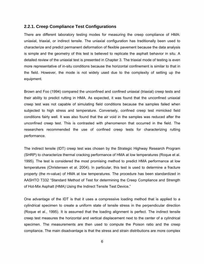
A typical relationship between the calculated total compliance and loading time is shown in

Figure 2.2. The creep compliance curve can be divided into three different parts (Witczak et al.,

2002):

• Primary creep: the portion wherein the strain rate decreases with loading time

• Secondary creep: the portion wherein the strain rate is constant with loading time

• Tertiary creep: the portion wherein the strain rate increases with loading time

A large increase in creep compliance occurs within the tertiary part. The point at which tertiary

deformation begins is defined as the flow time (FT). This has been found to be an important

parameter in evaluating HMA rutting resistance (Hafez, 1997). The flow time (FT) is defined as

the time at which the shear deformation under constant volume starts (Kim et al., 2002). The

8

flow time is also regarded as the minimum point of the rate of change for compliance to loading

time (Witczak et al., 2002).

Figure 2.2 Domains of the creep compliance

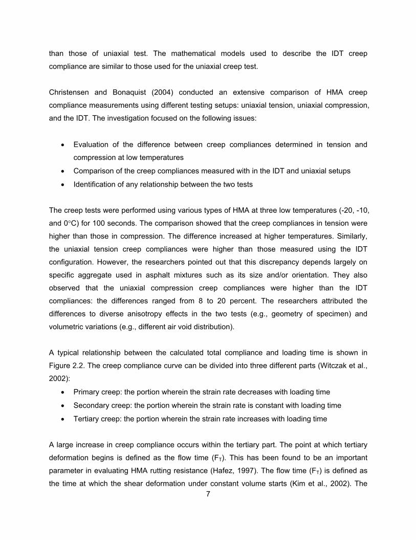
2.2.2. Creep Compliance Models

The two most commonly used mathematical models for representing the creep compliance

master curve (CCMC) are the power function and Prony series. The power models [Equation

(3)] are commonly used to analyze the secondary part of the CCMC when plotted on logarithmic

space as presented in Figure 2.3 (Kim et al., 2002).

0 1( ) mD t D D t= + (3)

where

D0 = instantaneous creep compliance,

D(t) = total creep compliance at any time,

t = loading time, and

D1, m = materials regression coefficients.

The regression coefficients D1 and m are commonly referred to as the compliance parameters.

The compliance value increases as either the D1 or m-value increases.

9

Figure 2.3 Regression constants D1 and m

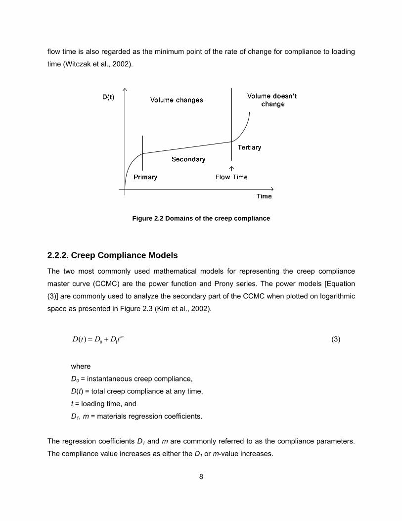
The other popular method used to model the creep compliance is the Prony series. This

approach uses the generalized Maxwell model analogy (Figure 2.4) to represent the viscoelastic

properties of the asphalt concrete mixture in relaxation. Hiltunen and Roque (1995) found that

this method is useful to represent the compliance because the Prony series simplifies the

interconversion between the creep compliance and relaxation modulus. The Prony series is

defined by the following equation:

/

1

( ) (1 )r i

nt

r g ii

D t D D e τ−

=

= + −∑ (4)

where

D(tr) = creep compliance at reduced time tr,

0lim ( )r

g rtD D t

→= = equilibrium (glassy) creep compliance,

tr = reduced time (t/aT),

aT = temperature shift factor, and

Di, iτ = Prony series parameters.

.

D(tr)

tr

D1

D0

D(tr) = D0 + D1trm

m 1

1

10

Figure 2.4 Generalized Maxwell model

2.3. The Relaxation Modulus

Stress relaxation of asphalt materials is a phenomenon similar to creep. In the creep test, a

constant loading to the material and an instant strain (ε0) occur causing the material to creep

with time. On the other hand, if the instant strain is fixed and remains constant, then the applied

stress will be relaxed. This reduction in stress over time is called stress relaxation and the

relaxation modulus is computed using Equation (5).

0

( )( ) tE t σε

= (5)

where

E(t) = relaxation modulus,

( )tσ = stress at any time, and

0ε = instantaneous strain.

The relaxation modulus is used to predict thermal stress in asphalt pavements. Thermal stress

in the pavement can be computed using the constitutive Equation (6), which explains the stress

development during cooling. This equation is based on Boltzmann’s superposition principle for

linear viscoelastic materials (Hiltunen et al. 1994).

11

0

( ) ( ') ''

rt

r r r rr

dt E t t dtdtεσ = −∫ (6)

where

σ(tr) = stress at reduced time tr,

E(tr - tr’) = relaxation modulus at reduced time tr - tr’,

ε = strain at reduced time tr, and

tr’ = variable of integration.

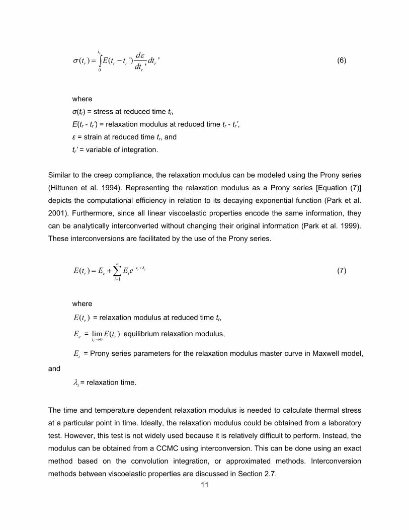
Similar to the creep compliance, the relaxation modulus can be modeled using the Prony series

(Hiltunen et al. 1994). Representing the relaxation modulus as a Prony series [Equation (7)]

depicts the computational efficiency in relation to its decaying exponential function (Park et al.

2001). Furthermore, since all linear viscoelastic properties encode the same information, they

can be analytically interconverted without changing their original information (Park et al. 1999).

These interconversions are facilitated by the use of the Prony series.

/

1

( ) r i

nt

r e ii

E t E E e λ−

=

= +∑ (7)

where

( )rE t = relaxation modulus at reduced time tr,

eE = 0

lim ( )r

rtE t

→ equilibrium relaxation modulus,

iE = Prony series parameters for the relaxation modulus master curve in Maxwell model,

and

iλ = relaxation time.

The time and temperature dependent relaxation modulus is needed to calculate thermal stress

at a particular point in time. Ideally, the relaxation modulus could be obtained from a laboratory

test. However, this test is not widely used because it is relatively difficult to perform. Instead, the

modulus can be obtained from a CCMC using interconversion. This can be done using an exact

method based on the convolution integration, or approximated methods. Interconversion

methods between viscoelastic properties are discussed in Section 2.7.

12

2.4. Time-Temperature Superposition and Master Curve

The response dependence on both time and temperature is evaluated for the characterization of

viscoelastic materials such as HMA. In general, creep tests are performed at various

temperatures. However, the time and temperature dependent creep response can be expressed

by a single parameter, reduced time (tr), using the time-temperature superposition principle

(Painter and Coleman, 1997). Data collected at different temperatures, -15, 5, 20, 30, and 40˚C

in this study, can be shifted to form a CCMC at a reference temperature (usually 20˚C). The

amount of shifting required at each temperature is called the shift factor, a(T), and is a constant

by which the loading times at each temperature can be divided to give a reduced loading time, tr,

for the master curve. The reduced time is calculated using the following Equation:

( )rtta T

= (8)

where

tr = reduced time of loading,

t = actual time of loading, and

a(T) = shift factor for data measured at temperature (T).

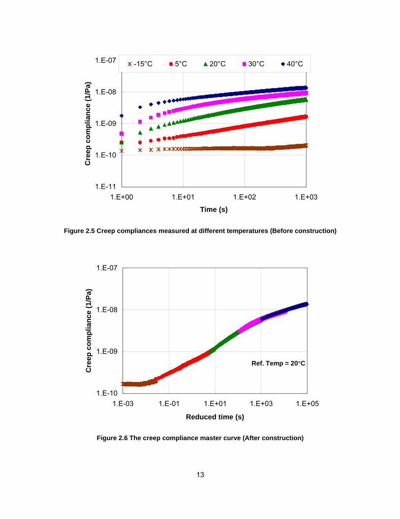
Creep compliances measured at temperatures below the reference temperature should be

shifted toward the left direction to construct a single smooth line of master curve as shown in

Figure 2.5 and Figure 2.6. This is because compliance values at temperatures lower than the

reference temperature should be lower than those at higher temperatures and vice versa.

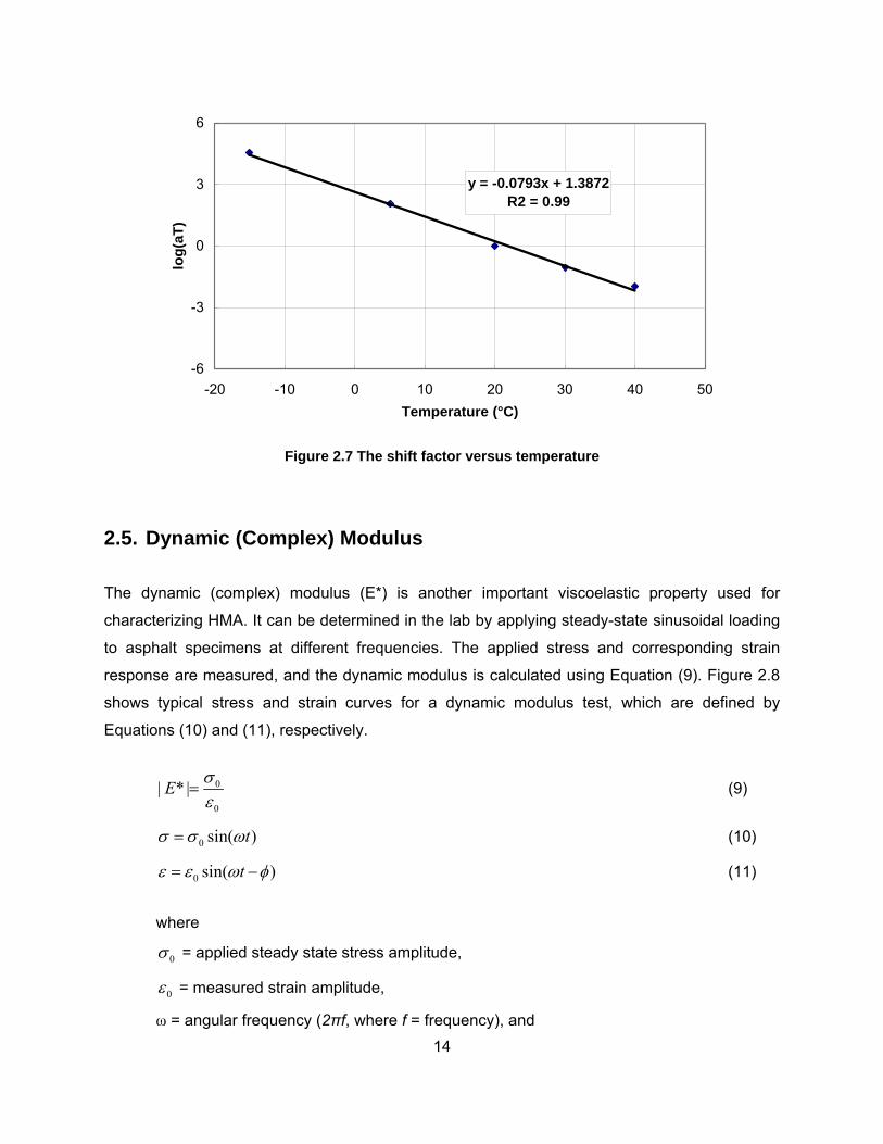
Figure 2.7 shows a typical relationship between the shift factor and temperatures on a semi-log

plot (from Figure 2.5 and Figure 2.6).

13

1.E-11

1.E-10

1.E-09

1.E-08

1.E-07

1.E+00 1.E+01 1.E+02 1.E+03

Time (s)

Cre

ep c

ompl

ianc

e (1

/Pa)

-15°C 5°C 20°C 30°C 40°C

Figure 2.5 Creep compliances measured at different temperatures (Before construction)

1.E-10

1.E-09

1.E-08

1.E-07

1.E-03 1.E-01 1.E+01 1.E+03 1.E+05

Reduced time (s)

Cre

ep c

ompl

ianc

e (1

/Pa)

Figure 2.6 The creep compliance master curve (After construction)

Ref. Temp = 20°C

14

y = -0.0793x + 1.3872R2 = 0.99

-6

-3

0

3

6

-20 -10 0 10 20 30 40 50Temperature (°C)

log(

aT)

Figure 2.7 The shift factor versus temperature

2.5. Dynamic (Complex) Modulus

The dynamic (complex) modulus (E*) is another important viscoelastic property used for

characterizing HMA. It can be determined in the lab by applying steady-state sinusoidal loading

to asphalt specimens at different frequencies. The applied stress and corresponding strain

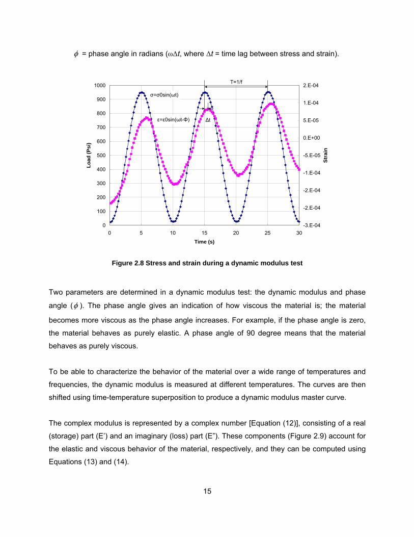
response are measured, and the dynamic modulus is calculated using Equation (9). Figure 2.8

shows typical stress and strain curves for a dynamic modulus test, which are defined by

Equations (10) and (11), respectively.

0

0

| * |E σε

= (9)

0 sin( )tσ σ ω= (10)

0 sin( )tε ε ω φ= − (11)

where

0σ = applied steady state stress amplitude,

0ε = measured strain amplitude,

ω = angular frequency (2πf, where f = frequency), and

15

φ = phase angle in radians (ω∆t, where ∆t = time lag between stress and strain).

0

100

200

300

400

500

600

700

800

900

1000

0 5 10 15 20 25 30

Time (s)

Load

(Psi

)

-3.E-04

-2.E-04

-2.E-04

-1.E-04

-5.E-05

0.E+00

5.E-05

1.E-04

2.E-04

Stra

in

T=1/f

∆tε=ε0sin(ωt-Φ)

σ=σ0sin(ωt)

Figure 2.8 Stress and strain during a dynamic modulus test

Two parameters are determined in a dynamic modulus test: the dynamic modulus and phase

angle (φ ). The phase angle gives an indication of how viscous the material is; the material

becomes more viscous as the phase angle increases. For example, if the phase angle is zero,

the material behaves as purely elastic. A phase angle of 90 degree means that the material

behaves as purely viscous.

To be able to characterize the behavior of the material over a wide range of temperatures and

frequencies, the dynamic modulus is measured at different temperatures. The curves are then

shifted using time-temperature superposition to produce a dynamic modulus master curve.

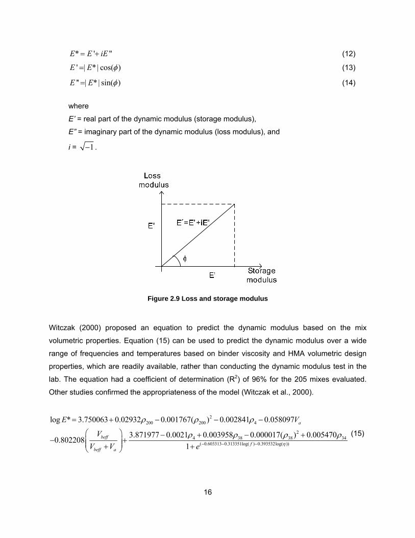
The complex modulus is represented by a complex number [Equation (12)], consisting of a real

(storage) part (E’) and an imaginary (loss) part (E”). These components (Figure 2.9) account for

the elastic and viscous behavior of the material, respectively, and they can be computed using

Equations (13) and (14).

16

* ' "E E iE= + (12)

' | * | cos( )E E φ= (13)

'' | * | sin( )E E φ= (14)

where

E’ = real part of the dynamic modulus (storage modulus),

E” = imaginary part of the dynamic modulus (loss modulus), and

i = 1− .

Figure 2.9 Loss and storage modulus

Witczak (2000) proposed an equation to predict the dynamic modulus based on the mix

volumetric properties. Equation (15) can be used to predict the dynamic modulus over a wide

range of frequencies and temperatures based on binder viscosity and HMA volumetric design

properties, which are readily available, rather than conducting the dynamic modulus test in the

lab. The equation had a coefficient of determination (R2) of 96% for the 205 mixes evaluated.

Other studies confirmed the appropriateness of the model (Witczak et al., 2000).

2

200 200 4

24 38 38 34

( 0.603313 0.313351log( ) 0.393532log( ))

log * 3.750063 0.02932 0.001767( ) 0.002841 0.058097

3.871977 0.0021 0.003958 0.000017( ) 0.0054700.8022081

a

befff

beff a

E V

VV V e η

ρ ρ ρ

ρ ρ ρ ρ− − −

= + − − −

⎛ ⎞ − + − +− +⎜ ⎟⎜ ⎟+ +⎝ ⎠

(15)

17

where

E* = dynamic modulus in psi,

η = bitumen viscosity in 106 Poise,

f = loading frequency in Hertz,

Va = air void content in percent,

Vbeff = effective bitumen content in percent,

34ρ = cumulative percent retained on the ¾ in sieve,

38ρ = cumulative percent retained on the 3/8 in sieve,

4ρ = cumulative percent retained on the No. 4 in sieve, and

200ρ = percent passing the No. 200 sieve.

2.6. Sigmoidal Functions for Modeling Mater Curves

Pellinen and Witczak (2002) proposed using a sigmoidal function [Equation (16)] for modeling

the dynamic modulus master curve. The sigmoidal function is fitted to the dynamic modulus test

data using regression analysis.

loglog *1 rf

Eeβ γ

αδ −= ++

(16)

where

log |E*| = log of the dynamic modulus,

fr = reduced frequency, and

α, β, γ, δ = fitting parameters.

This fitting function provides an analytically simple form that can be used to easily determine the

physical characteristics of a material at any temperature and loading time. Furthermore, the

equation parameters are of significance because they encode some meaningful information.

The parameters α and α+δ represent the minimum and maximum dynamic modulus values,

respectively. For example, the maximum dynamic modulus (α+δ) represents the maximum

stiffness of asphalt mixture, which at high temperature relies mainly on aggregate interlock, but

18

at intermediate and low temperatures depends also on the binder stiffness. The parameters β

and γ describe the shape of the sigmoidal function (Pellinen et al. 2002).

2.7. Interconversion among Viscoelastic Material Properties

Linear viscoelastic material properties (i.e., the creep compliance, relaxation modulus, complex

compliance, and dynamic modulus) can be converted to each other analytically because they

encode fundamentally the same information (Kim et al. 2002). This philosophy makes it possible

to predict one viscoelastic property from another. For instance, if the relaxation modulus is

needed but it is difficult to measure directly from a test, it would be convenient to predict it from

another viscoelastic property such as the creep compliance or dynamic modulus through

appropriate interconversion method (Schapery et al. 1999).

2.7.1. Interconversion between the Relaxation Modulus and Creep Compliance

Ferry (1980) showed that there is an exact relationship between the creep compliance and

relaxation modulus by using the convolution integral in Equation (17).

0( ) ( )

tE t D d tτ τ τ− =∫ for t>0 (17)

where

E(t) = relaxation modulus,

D(t) = creep compliance,

t = time, and

τ = integral variable.

When an analytical form of a viscoelastic material is not available and only data points

determined in the laboratory exist, the integral can be solved numerically (Park et al., 1999).

However, the numerical method requires significantly tedious and cumbersome work. For this

reason, researchers have proposed several approximate methods to convert linear viscoelastic

properties to each other. The simplest and crudest method is the quasi-elastic approximation

19

presented in Equation (18). Generally, this method is not applicable for typical viscoelastic

materials.

( ) ( ) 1E t D t ≅ , for t>0 (18)

Another approximate method can be used if both the creep compliance and relaxation modulus

are modeled using a power law analytical form. This method is based on Equation (19), which

was first proposed by Leaderman (1958). If the compliance and modulus can be expressed by a

power law model, which is drawn as a straight line on a logarithmic scale, then their relation is

simplified by the Laplace transformation. This transformation is capable of changing the integral

form of linear viscoelastic function into an algebraic form in the Laplace domain. It is noteworthy

that the exponent n of the power law model is the slope of the curve in the logarithmic plot. A

zero slope n indicates a material is purely elastic since there is no imaginary component.

sin( ) ( ) nE t D tnπ

π= (19)

where

1( ) nE t E t−= and

1( ) nD t D t= .

Practically, lab-determined data are not exactly represented by the power law function. However,

if the data does not perfectly follow a power model but the functions behave smoothly, Equation

(19) still works well. In this case, the local slope of the power model can be determined using

Equation (20) (Park et al. 1999). E(t) is interchangeable with D(t).

log ( )

logd E tnd t

= (20)

20

2.7.2. Interconversion between the Relaxation Modulus / Creep Compliance and Dynamic Modulus

Schapery and Park (1999) established analytical interconversion methods for linear viscoelastic

material properties using the Prony series. The researchers showed that if the time-dependent

functions are represented by the Prony series as in Equation (4) or (7), they can be analytically

converted into frequency-dependent functions (e.g., the dynamic modulus) using Equations (21)

through (24):

2 2

2 21

'( )1

mi i

ei i

EE E ω λωω λ=

= ++∑ (21)

2 2

2 21

"( )1

mi i

i i

EE ω λωω λ=

=+∑ (22)

2 21

'( )1

nj

gj j

DD Dω

ω τ=

= ++∑ (23)

2 21

"( )1

nj j

j j

DD

ωτω

ω τ=

=+∑ (24)

where

ω = angular frequency (2πf),

eE = 0

lim ( )r

rtE t

→ equilibrium relaxation modulus,

,i iE λ = Prony series parameters,

0lim ( )r

g rtD D t

→= equilibrium (glassy) creep compliance, and

Di, iτ = Prony series parameters.

For instance, if one has a set of lab-determined creep compliance data under transient loading

and it is represented by the Prony series, D’(ω) and D”(ω) are obtained through the relationship

expressed in Equations (23) and (24). Then, frequency dependent viscoelastic properties, both

the complex compliance (D*) and dynamic modulus (E*), can be determined as follows:

21

*( ) '( ) "( )D D iDω ω ω= − (25)

( ) ( )2 2*( ) '( ) "( )D D Dω ω ω= + (26)

*( ) *( ) 1E Dω ω = (27)

Schapery and Park (1999) also proposed approximate interconversion methods and verified

them using polymeric material represented by the Prony series. Equations (28) and (29) show

the formulas to convert between the dynamic modulus and relaxation modulus. These

relationships were derived based on the assumption that the time-dependent material is

represented by the power model (e.g., 1( ) nE t E t−= ). Therefore, if the source function can be

expressed by the power model, the method produces exact results. However, they can also be

used to produce an approximate solution using the slope of the curves at each point. This is the

same philosophy used for the approximate interconversion between the relaxation modulus and

creep compliance described in the previous section.

(1/ )'( ) ' ( )

tE E t

ωω λ

=≅ or

(1/ )

1( ) '( )' t

E t Eω

ωλ =

≅ (28)

(1/ )

"( ) " ( )t

E E tω

ω λ=

≅ or (1/ )

1( ) "( )" t

E t Eω

ωλ =

≅ (29)

where

λ’ = adjust function ( (1 )cos( / 2)n nπΓ − ),

λ” = adjust function ( (1 )sin( / 2)n nπΓ − ),

Γ = gamma function ( 1

0( ) n un u e du

∞ − −Γ = ∫ ), and

n = the local log-log slope of the storage moduluslog '( )

logd Ed

ωω

⎛ ⎞⎜ ⎟⎝ ⎠

.

2.8. Thermal Cracking Models

Several models have been proposed to predict thermal cracking on flexible pavements. In

general, they can be categorized into two groups: empirical-based models and mechanistic-

22

based models. The empirical models have been developed using statistical analyses, such as

the regression method, while the mechanistic models are based on the mechanics of materials

(Marasteanu et al., 2004).

2.8.1. Empirical-based Models for Thermal Cracking on Flexible Pavement

Most available empirical models were developed based on limited databases, thus, the

regression models often have low reliability. However, they allow determination of which

pavement characteristics have a significant effect on thermal cracking (Marasteanu et al., 2004).

A few examples are discussed below.

Fromm and Phang (1972) developed an empirical model to predict a cracking index based on

HMA, pavement and climate variables. The cracking index, used by the Ontario Department of

Transportation, evaluates the cracking severity based upon the number of transverse cracks.

Researchers measured the number and severity of cracks in 33 locations in Ontario, Canada

and developed transverse cracking prediction models using step-wise linear regression analysis.

They initially considered 40 variables; however, variables that did not have a significant effect

on the crack index were eliminated. Nine and eleven variables for general/southern and

northern models, respectively, were chosen to express the thermal cracking phenomenon. The

coefficient of determination (R2) for the models ranged from 0.64 to 0.70.

Hass et al. (1987) collected thermal cracking data, pavement characteristics and climatic

parameters at 25 airports in Canada and developed equations to predict the average spacing

between thermal cracks through step-wise statistical analyses. They concluded that low

temperature cracking at the airports depends largely on the influence of asphalt binder

characteristics in terms of PVN (McLeod’s Pen-Vis Number) or asphalt mixture characteristics

such as layer thickness and minimum temperature experienced. They also found that the PVN

values examined in their study ranged from 0.2 to -1.7. This was almost the same range for

unaged asphalt commonly used in Canada. The McLeod’s PVN is a correlation between asphalt

cement and the temperature susceptibility of the asphalt (McLeod, 1972).

23

2.8.2. Mechanistic-based Models

Researchers have also investigated the prediction of thermal cracking using mechanistic

principles. Although the mechanistic prediction models for the computation of thermal cracking

are more complicated than the empirical ones, they deal with the cracking phenomenon at a

more fundamental level.

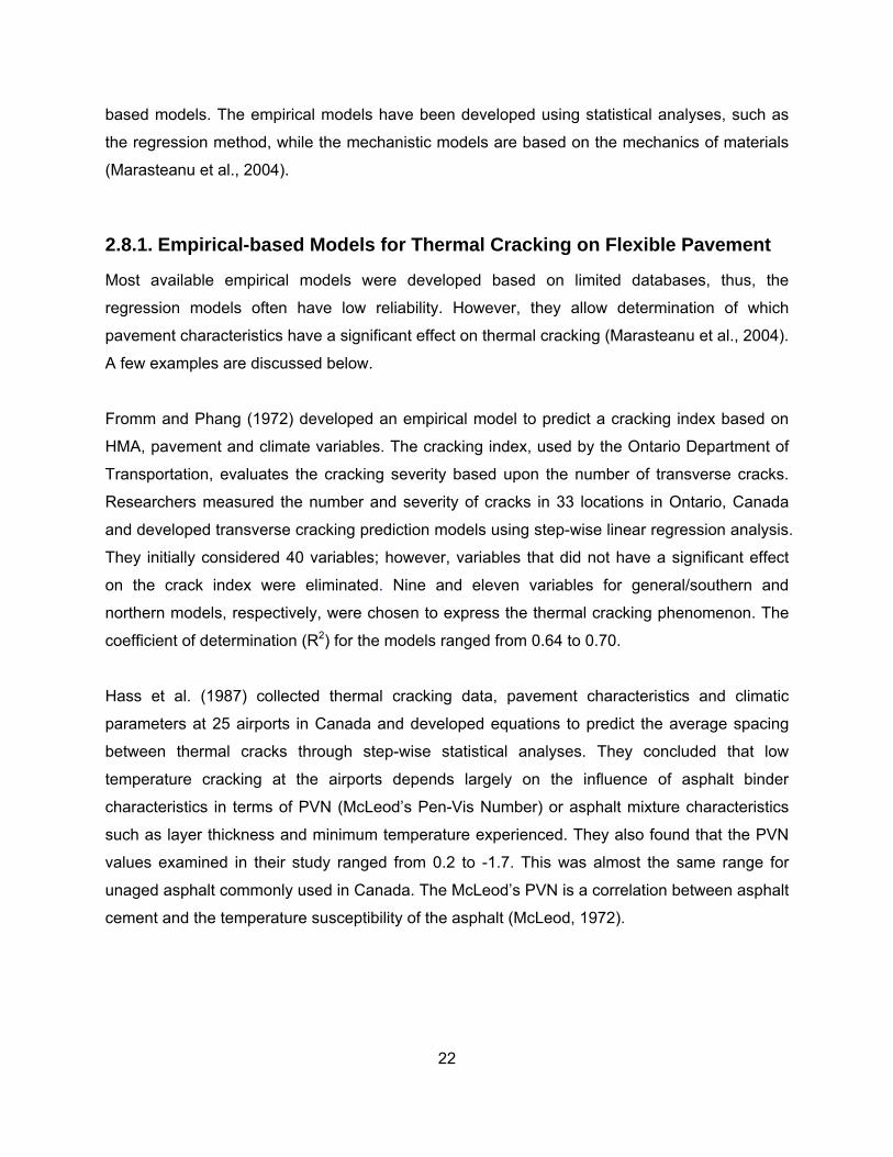
Hills and Brien (1966) first predicted the temperatures at which thermal cracks occur on the

surface of pavements. This study was based on the elastic behavior of asphalt material at low

temperatures. The researchers asserted that the fracture would occur when thermal stress and

thermal strength curves intercept (Figure 2.10). The thermal strength line assumes that tensile

strength of HMA is a function of its stiffness, citing Heukelom’s (1966) work. The researchers

assumed that the pavement behaves as an infinite beam or slab in order to calculate the

thermal stresses.

Figure 2.10 Estimating fracture temperature (After Hill and Brien, 1966)

Christison et al. (1972) employed five models to compare predicted and measured fracture

temperatures: Pseudo-elastic beam, approximate pseudo-elastic slab, viscoelastic beam,

viscoelastic slab, and approximate viscoelastic slab. Real field data was obtained from two test

roads constructed in Alberta and Manitoba, Canada in 1966 and 1967, respectively. The field

data provided a solid foundation to evaluate the considered stress predictive methods. The data

Stress and Strain

Temperature Estimated Fracture

Temp.

Thermal Stress

Thermal Strength

24

from the test roads suggested that a suitable pseudo-elastic beam analysis produces

reasonable results.

NCHRP Report 291 “Development of Pavement Structural Subsystems” (Finn et al., 1986)

produced a computer program named COLD (Computation of Low-Temperature Damage) to

predict when thermal cracking is likely to occur under known conditions such as temperature,

binder and layer thickness. The primary features of the program are the following:

• Temperature computation throughout the pavement structure

• Thermal stress computation on the surface of the asphalt pavement

• Comparison of tensile strength with thermal stress to predict thermal cracking

2.8.3. M-E Design Guide Model (2002)

As part of the SHRP A-005 contract, a new prediction model for thermal cracking over time was

developed (Witczak et al., 2000). The new method, which is called TCMODEL, uses mixture

properties measured from the IDT creep. Hiltunen and Roque (1995) described the primary

thermal cracking mechanism as presented in Figure 2.11:

Figure 2.11 Thermal cracking development mechanism

Since pavement temperature is lowest on the surface, there is a high probability that the tensile

stress would be maximal on the surface. Therefore, thermal cracking induced by temperature

should occur on the surface first. The thermal cracking model proposed by Hiltunen and Roque

has two primary components: (1) a mechanistic-based model that computes the propagation of

Cooling

Strain

Stress

Crack

Cooling induces contraction strains

Strains lead to thermal tensile stress in the surface layer

Thermal stress is greatest in the longitudinal direction of the pavement

Transverse cracks develop on the surface layer

25

each crack on a certain area of the surface, and (2) a probabilistic approach to compute the

gross amount of thermal cracks. Only the mechanistic-based model will be reviewed herein.

Linear elastic fracture mechanics were used to predict crack depth. The fracture model is shown

schematically in Figure 2.12. The change in the depth of thermal crack due to the cooling cycle

is computed using the Paris relationship presented in Equation (30).

( )nC A K∆ = ∆ (30)

where

∆C = change in crack depth due to a cooling cycle,

∆K = change in stress intensity factor due to a cooling cycle, and

A and n = empirically determined fracture parameters.

Figure 2.12 Schematic of crack depth model (after Hiltunen and Roque, 1995)

The parameter A can be determined using Equation (31), originally developed by Molenaar

(1983) and modified by Witczak et al. (2000). According to the hierarchical levels, the values of

5, 1.5, and 3 are recommended for the levels 1, 2, and 3 (Witczak et al., 2000), respectively.

( )log 4.389 2.52*log( * * )mA E nβ σ= − (31)

where

β = calibration parameter (5, 1.5 or 3 according to the hierarchical level),

E = mixture stiffness = 10000,

mσ = undamaged mixture tensile strength, and

n = empirically determined fracture parameter.

C0 C

∆C

Asphalt Surface Layer

Thermal

Stress

Distribution

26

The researchers recommend measuring the undamaged mixture tensile strength (σm) at -10°C.

The strength of an asphalt mixture increases with the decrease of temperature. However, below

a certain temperature, the strength starts to decrease because the mixture is damaged due to

excessive thermal stress. According to tensile tests using cored samples from the field, the

maximum tensile strength was usually below -10°C. However, for a conservative design, the

strength at -10°C is used to calculate the parameter A (Witczak et al., 2000).

Lytton et al. (1983) developed the following relationship to compute the n-value based on the m-

value obtained from modeling the linear part of a creep compliance test with a power model as

in Equation (3).

10.8 1nm

⎛ ⎞= +⎜ ⎟⎝ ⎠

(32)

where

m = the slope of the linear portion of the CCMC on a logarithmic scale.

27

Chapter 3 Experimental Program

3.1. Introduction

This chapter describes the experimental program conducted to achieve the objective of this

research. The discussion covers sample preparation, conditioning procedure, and creep tests

performed. Two sets of creep tests were conducted using uniaxial and indirect tensile creep

configurations. MTS and Interlaken servo-hydraulic machines were used to obtain creep data

for the IDT and uniaxial test, respectively. Both machines have environmental chambers to

constantly maintain a certain temperature.

3.2. Sample Preparation and Conditioning

The specimens were prepared at the VTTI asphalt laboratory. Two typical Virginia mixes were

used: a surface mix (SM 9.5A) and a base mix (BM 25.0). The mixes were designed according

to VDOT specifications (Flintsch et al., 2005). The mix design for the base course included

limestone aggregate, concrete sand, reclaimed asphalt pavement (RAP) and PG 64-22 asphalt

binder. The mix design for the surface course used quartzite aggregate, concrete sand, RAP,

and the same binder. The job mix formula (JMF) specified by VDOT and the source of the

aggregates for both mixes are shown in Table 3.1 and Table 3.2.

Three different samples with the same gradations were prepared for each mix using the

percentages presented. Sieve analysis in accordance with AASHTO T27 and T11 was

conducted in order to verify whether or not the gradations were acceptable. All the samples met

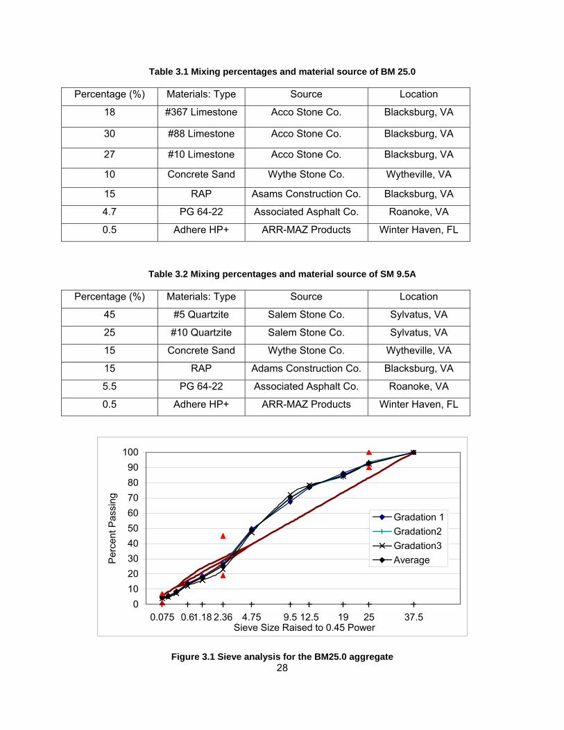
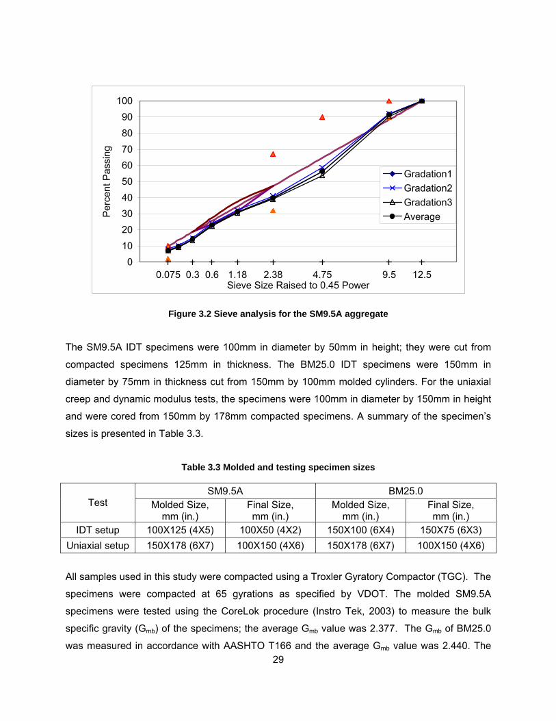
the gradation specifications limits. Figure 3.1 and Figure 3.2 show the 0.45 power gradations for

the BM25.0 and SM9.5A, respectively. The triangle marks indicate the upper and lower limits

according to the corresponding SUPERPAVE specifications.

28

Table 3.1 Mixing percentages and material source of BM 25.0

Percentage (%) Materials: Type Source Location

18 #367 Limestone Acco Stone Co. Blacksburg, VA

30 #88 Limestone Acco Stone Co. Blacksburg, VA

27 #10 Limestone Acco Stone Co. Blacksburg, VA

10 Concrete Sand Wythe Stone Co. Wytheville, VA

15 RAP Asams Construction Co. Blacksburg, VA

4.7 PG 64-22 Associated Asphalt Co. Roanoke, VA

0.5 Adhere HP+ ARR-MAZ Products Winter Haven, FL

Table 3.2 Mixing percentages and material source of SM 9.5A

Percentage (%) Materials: Type Source Location

45 #5 Quartzite Salem Stone Co. Sylvatus, VA

25 #10 Quartzite Salem Stone Co. Sylvatus, VA

15 Concrete Sand Wythe Stone Co. Wytheville, VA

15 RAP Adams Construction Co. Blacksburg, VA

5.5 PG 64-22 Associated Asphalt Co. Roanoke, VA

0.5 Adhere HP+ ARR-MAZ Products Winter Haven, FL

37.5251912.59.54.752.361.180.60.0750

102030405060708090

100

Sieve Size Raised to 0.45 Power

Per

cent

Pas

sing

Gradation 1Gradation2Gradation3Average

Figure 3.1 Sieve analysis for the BM25.0 aggregate

29

12.59.54.752.381.180.60.30.0750

102030405060708090

100

Sieve Size Raised to 0.45 Power

Per

cent

Pas

sing

Gradation1Gradation2Gradation3Average

Figure 3.2 Sieve analysis for the SM9.5A aggregate

The SM9.5A IDT specimens were 100mm in diameter by 50mm in height; they were cut from

compacted specimens 125mm in thickness. The BM25.0 IDT specimens were 150mm in

diameter by 75mm in thickness cut from 150mm by 100mm molded cylinders. For the uniaxial

creep and dynamic modulus tests, the specimens were 100mm in diameter by 150mm in height

and were cored from 150mm by 178mm compacted specimens. A summary of the specimen’s

sizes is presented in Table 3.3.

Table 3.3 Molded and testing specimen sizes

SM9.5A BM25.0 Test Molded Size,

mm (in.) Final Size, mm (in.)

Molded Size, mm (in.)

Final Size, mm (in.)

IDT setup 100X125 (4X5) 100X50 (4X2) 150X100 (6X4) 150X75 (6X3) Uniaxial setup 150X178 (6X7) 100X150 (4X6) 150X178 (6X7) 100X150 (4X6)

All samples used in this study were compacted using a Troxler Gyratory Compactor (TGC). The

specimens were compacted at 65 gyrations as specified by VDOT. The molded SM9.5A

specimens were tested using the CoreLok procedure (Instro Tek, 2003) to measure the bulk

specific gravity (Gmb) of the specimens; the average Gmb value was 2.377. The Gmb of BM25.0

was measured in accordance with AASHTO T166 and the average Gmb value was 2.440. The

30

maximum theoretical specific gravity (Gmm) for both mixes was determined in accordance with

AASHTO T209; the average of the Gmm were 2.467 and 2.601 for the SM and BM, respectively.

The specimens for the dynamic modulus and uniaxial creep tests were not compacted using a

fixed number of gyrations. The specimen weight for the specified testing size (6 in X 7 in) with

4% of air voids was calculated from the measured Gmm values and the specimens were

compacted using a variable number of gyrations until reaching the required height. The average

measured values of Gmb and VTM(%) for all specimens used in this research are presented in

Table 3.4. It must be noted that these values are for the molded specimens rather than for the

cored specimens; which are usually slightly different. Two specimens were tested at each

temperature to measure the variability among tested specimens. The testing conditions and

sample numbering are summarized in Table 3.5.

Table 3.4 VTM and Gmb for molded specimens

VTM (%) Gmb Test type

SM BM SM BM

Dynamic Modulus 4.2 5.0 2.365 2.365

Uniaxial Creep 4.3 5.1 2.365 2.365

IDT Creep 3.6 6.2 2.377 2.440

Table 3.5 Summary of test specimens for creep analysis

Temperature (°C) Test Mix

-15 5 20 30 40

S109 S110 S113 S114 S117 SM S111 S112 S115 S116 S119 B78 B79 B60 B61 B55

Uniaxial BM

B81 B80 B84 B85 B58 S59 S60 S61 S62 S63 SM S66 S67 S68 S69 S70 B31 B32 B33 B35 B36

IDT BM

B34 B37 B40 B38 B41 S93 S94 S97 S98 S105 SM S95 S96 S101 S102 S107 B62 B63 B68 B69 B56

Dynamic Modulus BM

B64 B65 B76 B77 B67

31

3.3. Test Methods

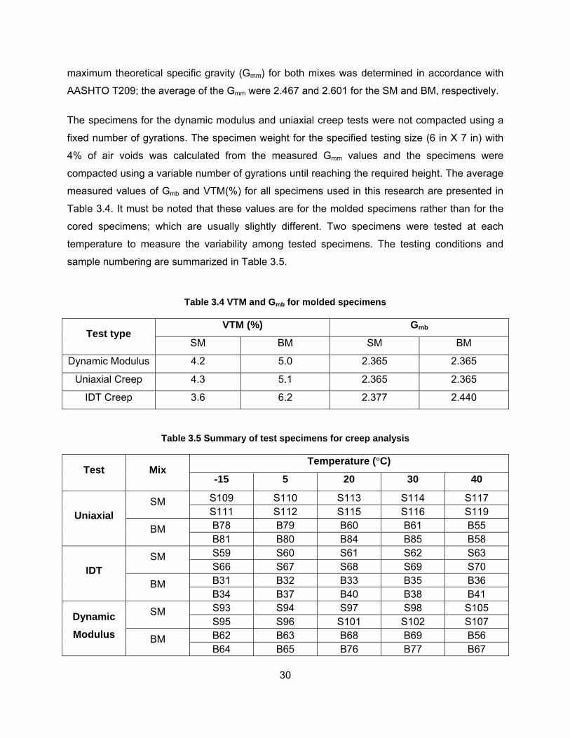
3.3.1. Uniaxial Creep Test

In the uniaxial creep test, the strain-time relationship was measured in an unconfined condition.

The set-up for the uniaxial creep testing is shown in Figure 3.3. An environmental chamber

maintains the samples at a certain temperature to an accuracy of ±0.5˚C. Before the test is

performed, samples are conditioned in the chamber for three hours in order to stabilize the

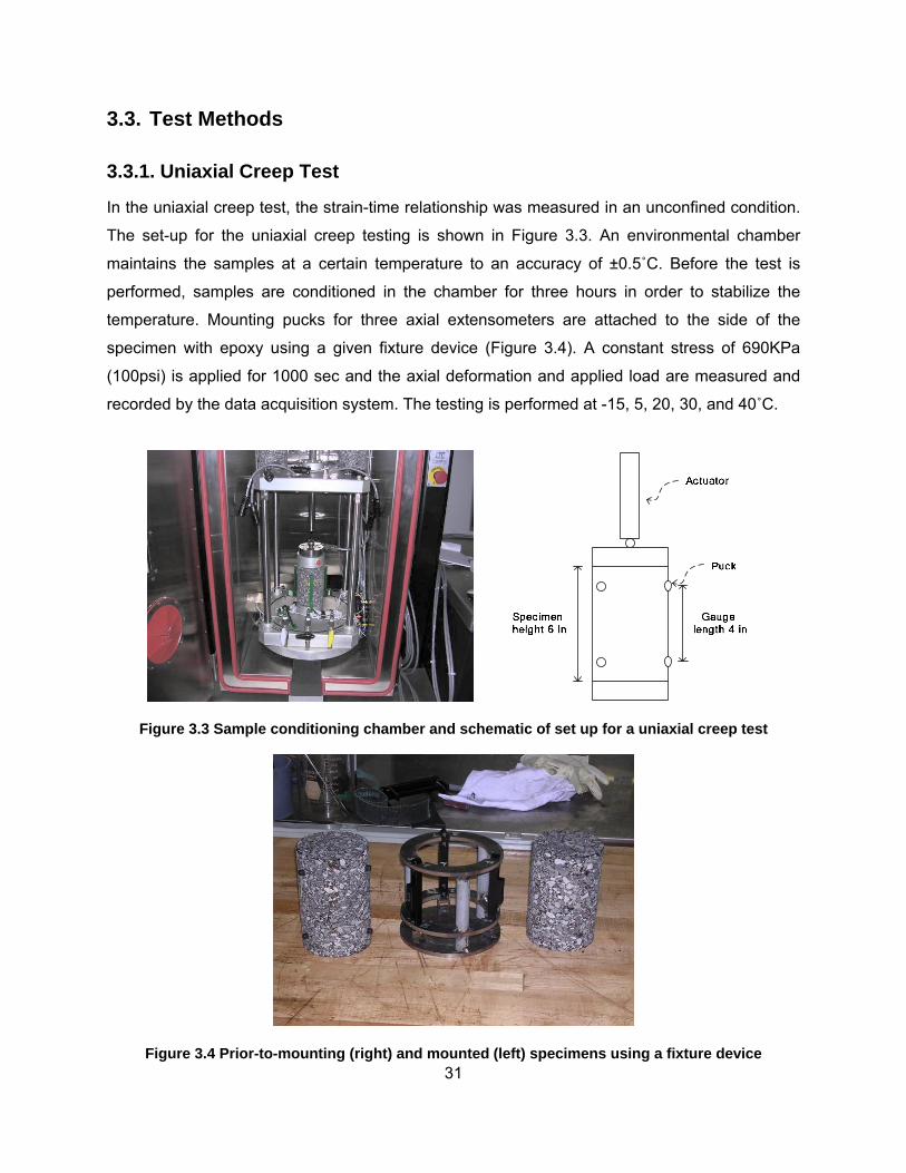
temperature. Mounting pucks for three axial extensometers are attached to the side of the

specimen with epoxy using a given fixture device (Figure 3.4). A constant stress of 690KPa

(100psi) is applied for 1000 sec and the axial deformation and applied load are measured and

recorded by the data acquisition system. The testing is performed at -15, 5, 20, 30, and 40˚C.

Figure 3.3 Sample conditioning chamber and schematic of set up for a uniaxial creep test

Figure 3.4 Prior-to-mounting (right) and mounted (left) specimens using a fixture device

32

The computer system automatically computes the average axial deformation by averaging the

readings from the three LVDTs. The average deformation values are converted to total axial

strain by dividing by the gauge length. (L = 4 in). The total axial compliance [D(t)] is then

calculated using Equation (1). The total axial compliance over time is plotted in a logarithmic

scale.

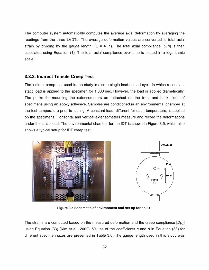
3.3.2. Indirect Tensile Creep Test

The indirect creep test used in the study is also a single load-unload cycle in which a constant

static load is applied to the specimen for 1,000 sec. However, the load is applied diametrically.

The pucks for mounting the extensometers are attached on the front and back sides of

specimens using an epoxy adhesive. Samples are conditioned in an environmental chamber at

the test temperature prior to testing. A constant load, different for each temperature, is applied

on the specimens. Horizontal and vertical extensometers measure and record the deformations

under the static load. The environmental chamber for the IDT is shown in Figure 3.5, which also

shows a typical setup for IDT creep test.

Figure 3.5 Schematic of environment and set up for an IDT

The strains are computed based on the measured deformation and the creep compliance [D(t)]

using Equation (33) (Kim et al., 2002). Values of the coefficients c and d in Equation (33) for

different specimen sizes are presented in Table 3.6. The gauge length used in this study was

33

30mm. The corresponding values of c and e were calculated using the Matlab software and the

formula proposed by Kim et al. (2002).

[ ]( ) ( ) ( )dD t cU t eV tP

= − + (33)

where

d = the thickness of the test specimen (mm),

P = the applied load (psi),

c, d = coefficients related to geometry of the specimen,

U(t) = horizontal strain (mm), and

V(t) = vertical strain (mm).

Table 3.6 Coefficients used to calculate the creep compliance (Kim at el., 2002)

Specimen diameter (mm)

Gauge Length

(mm) c e

27.4 0.7874 2.2783

30.0 0.6599 1.8710 100

50.8 0.4032 1.024

27.4 1.199 3.533

30.0 0.9874 2.8821

50.8 0.611 1.685 150

76.2 0.415 1.034

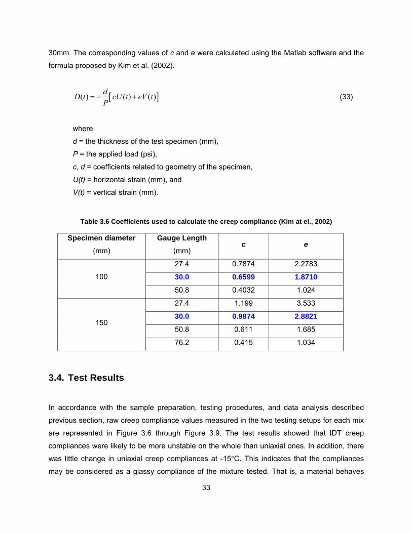
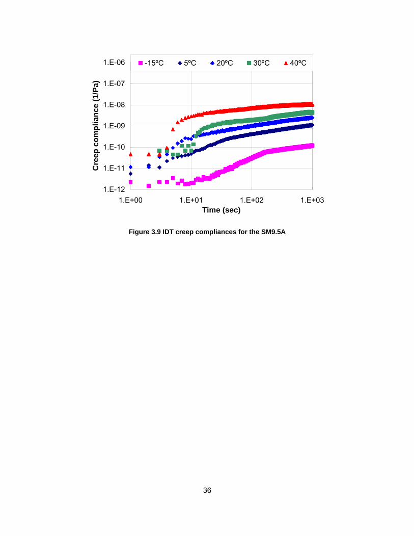
3.4. Test Results

In accordance with the sample preparation, testing procedures, and data analysis described

previous section, raw creep compliance values measured in the two testing setups for each mix

are represented in Figure 3.6 through Figure 3.9. The test results showed that IDT creep

compliances were likely to be more unstable on the whole than uniaxial ones. In addition, there

was little change in uniaxial creep compliances at -15°C. This indicates that the compliances

may be considered as a glassy compliance of the mixture tested. That is, a material behaves

34

elastically at the temperature. On the other hand, the IDT creep compliances at -15°C are still

changing over time tested. This is because tensile strains exist in the IDT setup creep test.

Tensile strain is prone to occur although the applied loading magnitude is relatively low and

Equation (33) considers both vertical and tensile strains. In the uniaxial setup, however, only

vertical strain occurs when a loading is applied and only the vertical strain is considered when

compliances are computed.

Moreover, the results show that there was a significant region of overlap between adjacent

temperatures from 20 to 40°C except for the IDT creep test for BM25.0. In contrast, there was a

relatively considerable gap between -15 and 20°C, even if the creep curves had still an

overlapped region. To construct a reliable CCMC, a sufficiently overlapped region between

adjacent creep compliance curves is necessary. However, more reliable CCMC could be

constructed if the overlapped regions between adjacent temperatures are similar.

1.E-11

1.E-10

1.E-09

1.E-08

1.E-07

1.E+00 1.E+01 1.E+02 1.E+03Time (s)

Cre

ep c

ompl

ianc

e (1

/Pa)

-15C 5C 20C 30C 40C

Figure 3.6 Uniaxial creep compliances for the BM25.0

35

1.E-11

1.E-10

1.E-09

1.E-08

1.E-07

1.E+00 1.E+01 1.E+02 1.E+03

Time (s)

Cre

ep c

ompl

ianc

e (1

/Pa)

-15°C 5°C 20°C 30°C 40°C

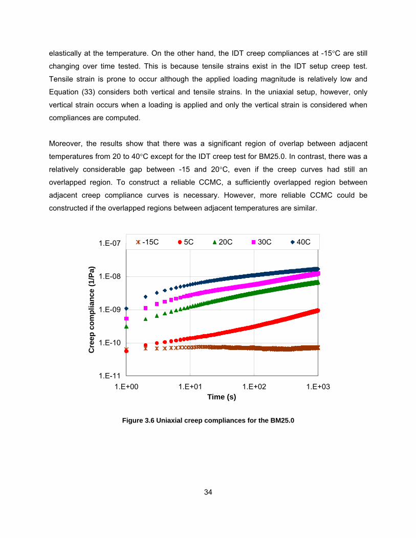
Figure 3.7 Uniaxial creep compliances for the SM9.5A

1.E-12

1.E-11

1.E-10

1.E-09

1.E-08

1.E-07

1.E-06

1.E+00 1.E+01 1.E+02 1.E+03Time (sec)

Cre

ep c

ompl

ianc

e (1

/Pa)

-15ºC 5ºC 20ºC 30ºC 40ºC

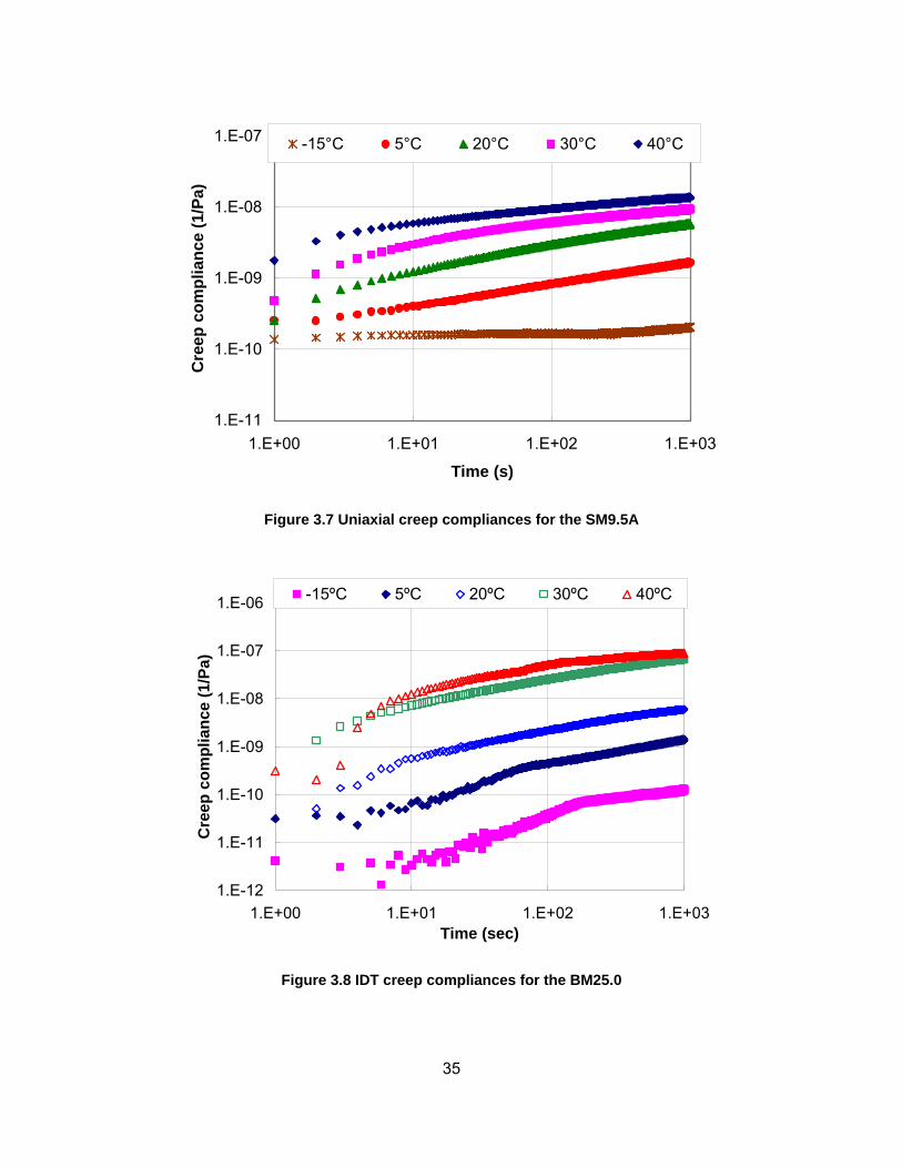
Figure 3.8 IDT creep compliances for the BM25.0

36

1.E-12

1.E-11

1.E-10

1.E-09

1.E-08

1.E-07

1.E-06

1.E+00 1.E+01 1.E+02 1.E+03Time (sec)

Cre

ep c

ompl

ianc

e (1

/Pa)

-15ºC 5ºC 20ºC 30ºC 40ºC

Figure 3.9 IDT creep compliances for the SM9.5A

37

Chapter 4 Creep Compliance Master Curves

4.1. Introduction

This chapter presents the analysis of the creep compliance tests conducted using the uniaxial

and IDT setups. The tests were conducted at five different temperatures: -15, 5, 20, 30, and

40°C. After obtaining individual creep compliance values for 1000 sec at each temperature, the

curves were shifted to a reference temperature of 20°C to produce one single smooth curve, the

creep compliance master curve (CCMC). Several models were then fitted to the data and the

slope of the power model in the logarithmic scale (m-value) was used to compare the

susceptibility of the mixes to thermal cracking.

4.2. Fitting Creep Compliance Master Curve Models

This section discusses the shifting of the individual creep compliance curves to construct the

CCMC and the various mathematical functions used to model the resulting data. Three

mathematical functions were investigated: the Prony series, sigmoidal, and power functions.

4.2.1. CCMC Construction

A convenient way to determine the shift factors is to visually shift the creep curve at various

temperatures to produce a “smooth” CCMC. This hand shifting method might be arguable

because it would appear to cause considerable errors in constructing CCMC. However, Witczak

et al. (2000) compared shift factors determined manually with those determined by a computer

program (MASTER). The software was developed for the automation of the construction of

CCMC as part of NCHRP 9-19 project. The comparison showed that there is little difference

between the automatic and manual procedures if the manual shifting is conducted with the aid

of a computerized spreadsheet (e.g., EXCEL). The spreadsheet facilitates the trial-and-error

process by showing the fit graphically.

38

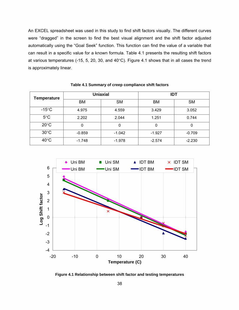
An EXCEL spreadsheet was used in this study to find shift factors visually. The different curves

were “dragged” in the screen to find the best visual alignment and the shift factor adjusted

automatically using the “Goal Seek” function. This function can find the value of a variable that

can result in a specific value for a known formula. Table 4.1 presents the resulting shift factors

at various temperatures (-15, 5, 20, 30, and 40°C). Figure 4.1 shows that in all cases the trend

is approximately linear.

Table 4.1 Summary of creep compliance shift factors

Uniaxial IDT Temperature

BM SM BM SM

-15°C 4.975 4.559 3.429 3.052

5°C 2.202 2.044 1.251 0.744

20°C 0 0 0 0

30°C -0.859 -1.042 -1.927 -0.709

40°C -1.748 -1.978 -2.574 -2.230

-4

-3

-2

-1

0

1

2

3

4

5

6

-20 -10 0 10 20 30 40Temperature (C)

Log

Shift

fact

or

Uni BM Uni SM IDT BM IDT SMUni BM Uni SM IDT BM IDT SM

Figure 4.1 Relationship between shift factor and testing temperatures

39

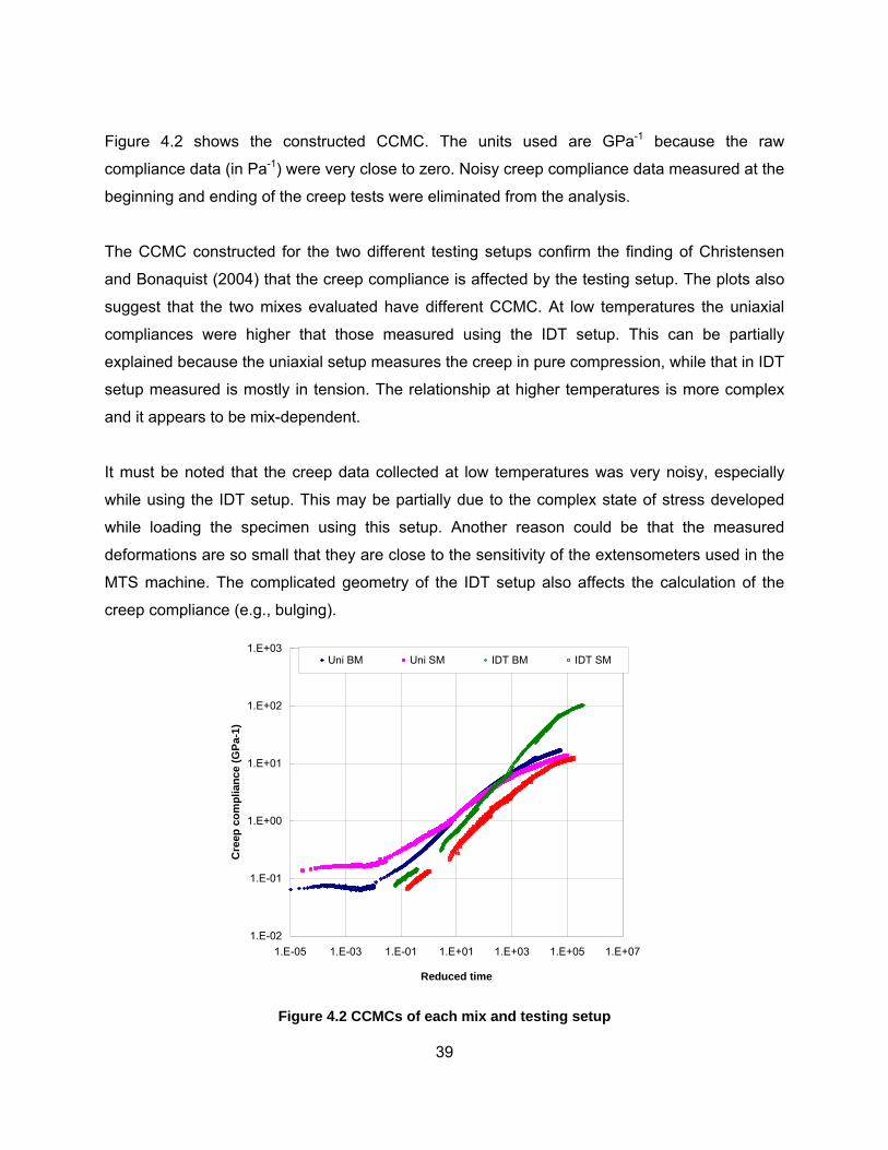
Figure 4.2 shows the constructed CCMC. The units used are GPa-1 because the raw

compliance data (in Pa-1) were very close to zero. Noisy creep compliance data measured at the

beginning and ending of the creep tests were eliminated from the analysis.

The CCMC constructed for the two different testing setups confirm the finding of Christensen

and Bonaquist (2004) that the creep compliance is affected by the testing setup. The plots also

suggest that the two mixes evaluated have different CCMC. At low temperatures the uniaxial

compliances were higher that those measured using the IDT setup. This can be partially

explained because the uniaxial setup measures the creep in pure compression, while that in IDT

setup measured is mostly in tension. The relationship at higher temperatures is more complex

and it appears to be mix-dependent.

It must be noted that the creep data collected at low temperatures was very noisy, especially

while using the IDT setup. This may be partially due to the complex state of stress developed

while loading the specimen using this setup. Another reason could be that the measured

deformations are so small that they are close to the sensitivity of the extensometers used in the

MTS machine. The complicated geometry of the IDT setup also affects the calculation of the

creep compliance (e.g., bulging).

1.E-02

1.E-01

1.E+00

1.E+01

1.E+02

1.E+03

1.E-05 1.E-03 1.E-01 1.E+01 1.E+03 1.E+05 1.E+07

Reduced time

Cre

ep c

ompl

ianc

e (G

Pa-1

)

Uni BM Uni SM IDT BM IDT SM

Figure 4.2 CCMCs of each mix and testing setup

40

4.2.2. CCMC Mathematical Model Fitting

The Prony Series Model One of the methods used to represent viscoelastic properties is to use decaying exponential

representation, commonly called “Prony” or “Dirichlet” series (Park and Kim 2001). As

previously described, the Prony series is based on the Maxwell model. The Prony series

increases its prediction capabilities as the number of terms is increased. However, at some

point the higher order coefficient stops being statistically significant.

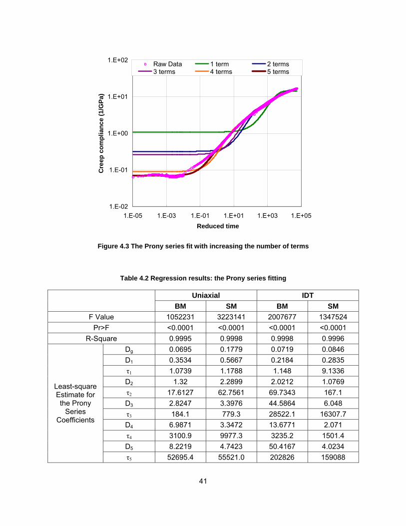
Figure 4.3 shows the Prony series fit with one to five terms for a BM25.0 uniaxial CCMC. The

coefficients were determined using the SAS software package. It must be noted that the least-

square fit was done on an arithmetic scale and for that reason the fit at low reduced times (very

small creep compliances) is very poor for the models with lower numbers of terms. A six-term

Prony series was also tried but the additional coefficients were not statistically significant. Thus,

a five-term model [Equation (34)] was selected.

5

/

1

( ) (1 )r itr g i

i

D t D D e τ−

=

= + −∑ (34)

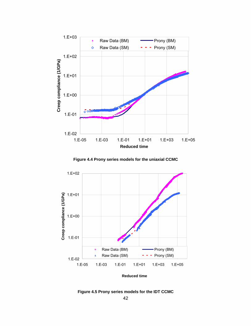
Table 4.2 summarizes the non-linear regression results for the Prony series model. The

statistical Prony series models are compared with the shifted CCMC data in Figure 4.4 and

Figure 4.5, for the BM25.0 and SM9.5A mixes, respectively. As expected, in general the models

follow the measured data closely.

The Prony series model for the uniaxial CCMC follows the experimental data closely, although

the fitted Prony series curves are a little wavy in the logarithmic scale. On the other hand, the

differences between the statistical predictions and experimental IDT CCMC are higher at low

temperatures. This could be explained by the measurement and data analysis limitations

presented earlier in the section.

41

1.E-02

1.E-01

1.E+00

1.E+01

1.E+02

1.E-05 1.E-03 1.E-01 1.E+01 1.E+03 1.E+05Reduced time

Cre

ep c

ompl

ianc

e (1

/GPa

)

Raw Data 1 term 2 terms3 terms 4 terms 5 terms

Figure 4.3 The Prony series fit with increasing the number of terms

Table 4.2 Regression results: the Prony series fitting

Uniaxial IDT

BM SM BM SM F Value 1052231 3223141 2007677 1347524

Pr>F <0.0001 <0.0001 <0.0001 <0.0001 R-Square 0.9995 0.9998 0.9998 0.9996

Dg 0.0695 0.1779 0.0719 0.0846 D1 0.3534 0.5667 0.2184 0.2835 τ1 1.0739 1.1788 1.148 9.1336 D2 1.32 2.2899 2.0212 1.0769 τ2 17.6127 62.7561 69.7343 167.1 D3 2.8247 3.3976 44.5864 6.048 τ3 184.1 779.3 28522.1 16307.7 D4 6.9871 3.3472 13.6771 2.071 τ4 3100.9 9977.3 3235.2 1501.4 D5 8.2219 4.7423 50.4167 4.0234

Least-square Estimate for the Prony

Series Coefficients

τ5 52695.4 55521.0 202826 159088

42

1.E-02

1.E-01

1.E+00

1.E+01

1.E+02

1.E+03

1.E-05 1.E-03 1.E-01 1.E+01 1.E+03 1.E+05Reduced time

Cre

ep c

ompl

ianc

e (1

/GPa

)

Raw Data (BM) Prony (BM)Raw Data (SM) Prony (SM)

Figure 4.4 Prony series models for the uniaxial CCMC

1.E-02

1.E-01

1.E+00

1.E+01

1.E+02

1.E-05 1.E-03 1.E-01 1.E+01 1.E+03 1.E+05

Reduced time

Cre

ep c

ompl

ianc

e (1

/GPa

)

Raw Data (BM) Prony (BM)Raw Data (SM) Prony (SM)

Figure 4.5 Prony series models for the IDT CCMC

43

The Sigmoidal Model Pellinen and Witczak (2002) proposed a sigmoidal function for modeling the dynamic modulus

master curve. In this investigation the sigmoidal model was also used for fitting the CCMC data

obtained from both testing setups. The sigmoidal function is presented in Equation (35):

loglog ( )1 rr tD teβ γ

αδ += −+

(35)

Coefficients of the model have meaningful physical significance (Figure 4.6). For instance, the

coefficients of β and γ determine the shape of the sigmoidal function model. A sigmoidal

functional curve will move to the left and become stiffer with the increase of β and γ ,

respectively. The coefficient δ α− and δ represent the minimum and maximum values of the

creep compliance, respectively. The coefficient δ α− represents the equilibrium (glassy)

compliance at very small times [0

lim ( )g tD D t

→= ].

Figure 4.6 Effect of the sigmoidal function coefficients on the CCMC

(After Pellinen and Witczak, 2002)

γ

δ (Maximum)

δ α− (Minimum)

β (Increase) β (Decrease)

(Increase)

log D(tr)

Reduced time (tr)

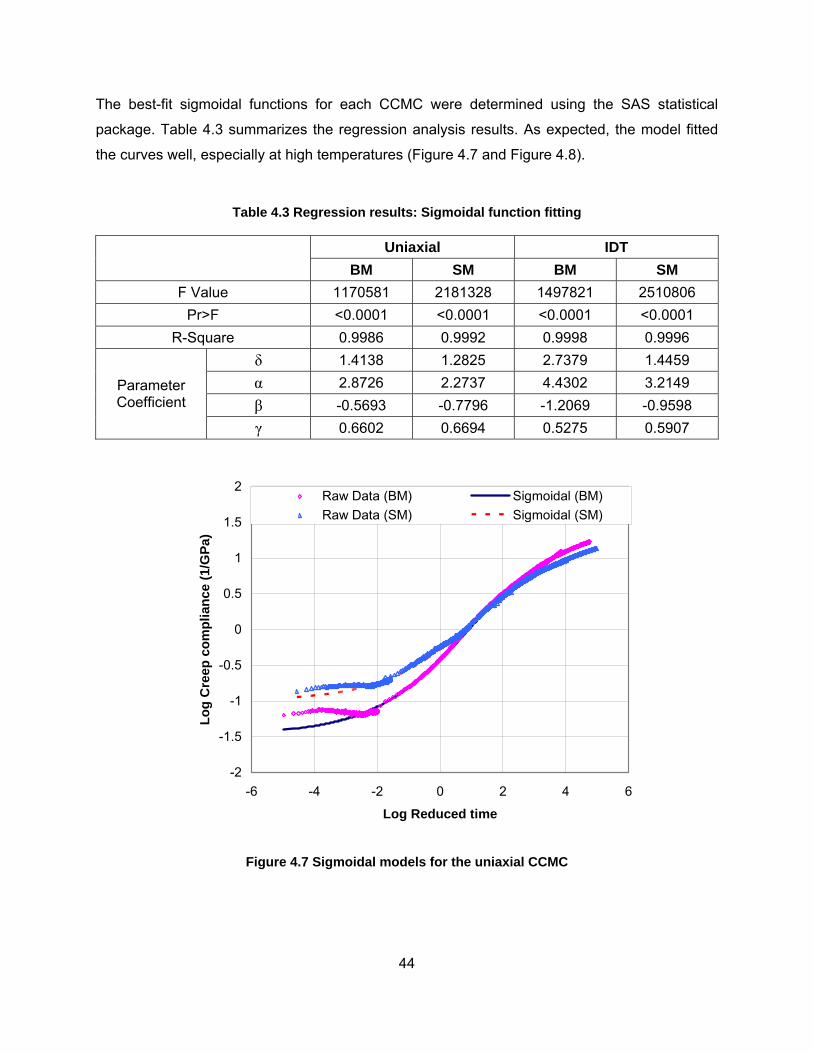
44

The best-fit sigmoidal functions for each CCMC were determined using the SAS statistical

package. Table 4.3 summarizes the regression analysis results. As expected, the model fitted

the curves well, especially at high temperatures (Figure 4.7 and Figure 4.8).

Table 4.3 Regression results: Sigmoidal function fitting

Uniaxial IDT

BM SM BM SM F Value 1170581 2181328 1497821 2510806

Pr>F <0.0001 <0.0001 <0.0001 <0.0001 R-Square 0.9986 0.9992 0.9998 0.9996

δ 1.4138 1.2825 2.7379 1.4459 α 2.8726 2.2737 4.4302 3.2149 β -0.5693 -0.7796 -1.2069 -0.9598

Parameter Coefficient

γ 0.6602 0.6694 0.5275 0.5907

-2

-1.5

-1

-0.5

0

0.5

1

1.5

2

-6 -4 -2 0 2 4 6

Log Reduced time

Log

Cre

ep c

ompl

ianc

e (1

/GPa

)

Raw Data (BM) Sigmoidal (BM)Raw Data (SM) Sigmoidal (SM)

Figure 4.7 Sigmoidal models for the uniaxial CCMC

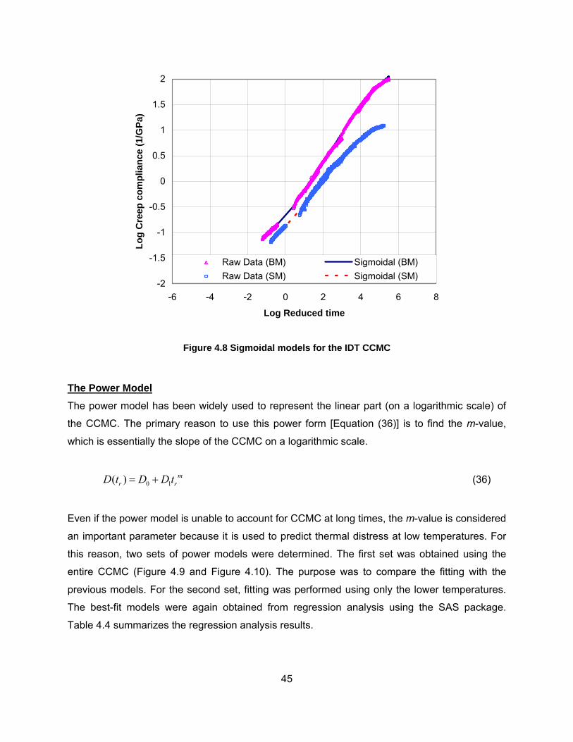
45

-2

-1.5

-1

-0.5

0

0.5

1

1.5

2

-6 -4 -2 0 2 4 6 8

Log Reduced time

Log

Cre

ep c

ompl

ianc

e (1

/GPa

)

Raw Data (BM) Sigmoidal (BM)Raw Data (SM) Sigmoidal (SM)

Figure 4.8 Sigmoidal models for the IDT CCMC

The Power Model The power model has been widely used to represent the linear part (on a logarithmic scale) of

the CCMC. The primary reason to use this power form [Equation (36)] is to find the m-value,

which is essentially the slope of the CCMC on a logarithmic scale.

0 1( ) mr rD t D D t= + (36)

Even if the power model is unable to account for CCMC at long times, the m-value is considered

an important parameter because it is used to predict thermal distress at low temperatures. For

this reason, two sets of power models were determined. The first set was obtained using the

entire CCMC (Figure 4.9 and Figure 4.10). The purpose was to compare the fitting with the

previous models. For the second set, fitting was performed using only the lower temperatures.

The best-fit models were again obtained from regression analysis using the SAS package.

Table 4.4 summarizes the regression analysis results.

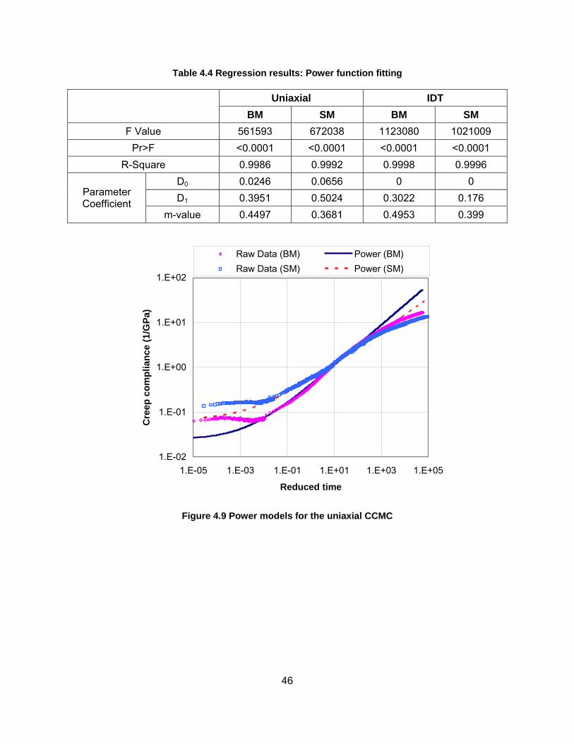
46

Table 4.4 Regression results: Power function fitting

Uniaxial IDT

BM SM BM SM F Value 561593 672038 1123080 1021009

Pr>F <0.0001 <0.0001 <0.0001 <0.0001 R-Square 0.9986 0.9992 0.9998 0.9996

D0 0.0246 0.0656 0 0 D1 0.3951 0.5024 0.3022 0.176 Parameter

Coefficient m-value 0.4497 0.3681 0.4953 0.399

1.E-02

1.E-01

1.E+00

1.E+01

1.E+02

1.E-05 1.E-03 1.E-01 1.E+01 1.E+03 1.E+05

Reduced time

Cre

ep c

ompl

ianc

e (1

/GPa

)

Raw Data (BM) Power (BM)Raw Data (SM) Power (SM)

Figure 4.9 Power models for the uniaxial CCMC

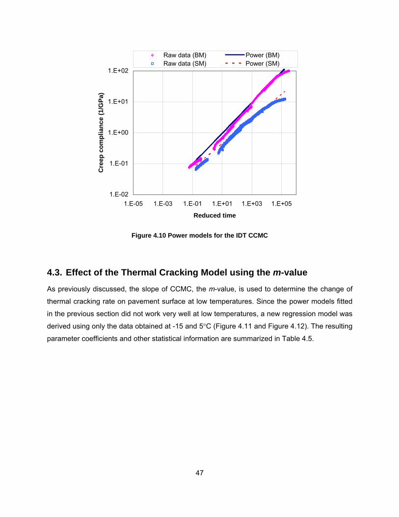
47

1.E-02

1.E-01

1.E+00

1.E+01

1.E+02

1.E-05 1.E-03 1.E-01 1.E+01 1.E+03 1.E+05

Reduced time

Cre

ep c

ompl

ianc

e (1

/GPa

)

Raw data (BM) Power (BM)Raw data (SM) Power (SM)

Figure 4.10 Power models for the IDT CCMC

4.3. Effect of the Thermal Cracking Model using the m-value

As previously discussed, the slope of CCMC, the m-value, is used to determine the change of

thermal cracking rate on pavement surface at low temperatures. Since the power models fitted

in the previous section did not work very well at low temperatures, a new regression model was

derived using only the data obtained at -15 and 5°C (Figure 4.11 and Figure 4.12). The resulting

parameter coefficients and other statistical information are summarized in Table 4.5.

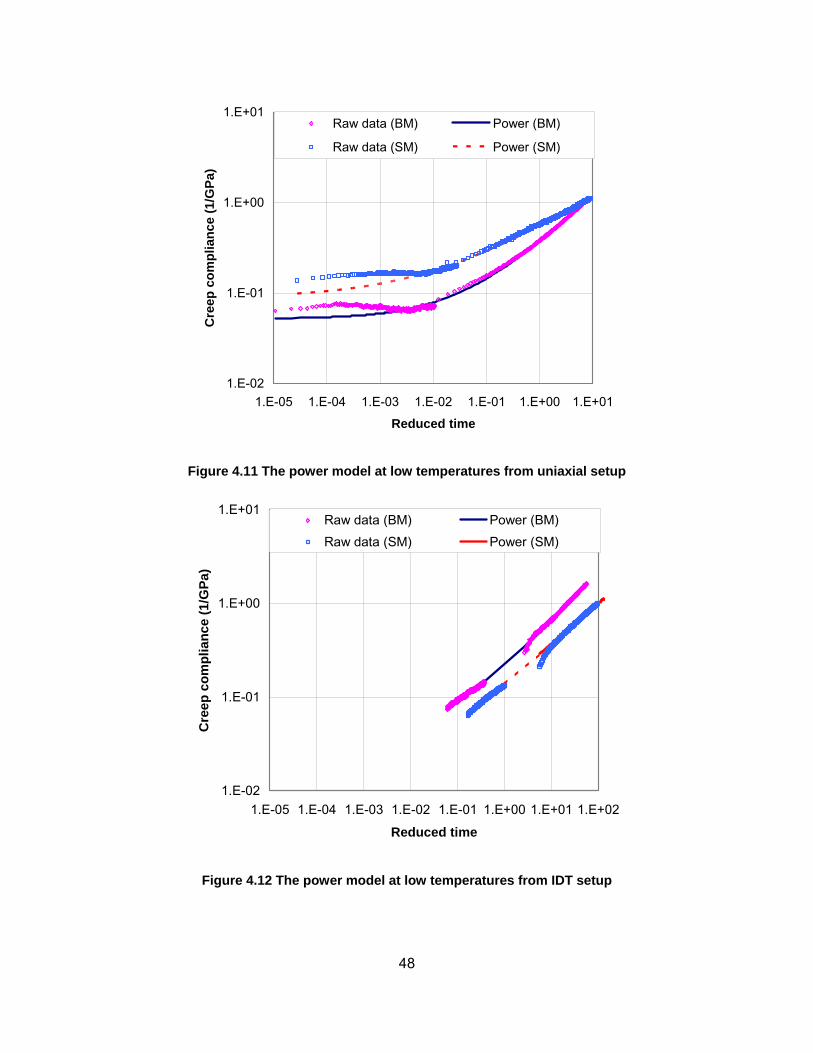
48

1.E-02

1.E-01

1.E+00

1.E+01

1.E-05 1.E-04 1.E-03 1.E-02 1.E-01 1.E+00 1.E+01

Reduced time

Cre

ep c

ompl

ianc

e (1

/GPa

)

Raw data (BM) Power (BM)

Raw data (SM) Power (SM)

Figure 4.11 The power model at low temperatures from uniaxial setup

1.E-02

1.E-01

1.E+00

1.E+01

1.E-05 1.E-04 1.E-03 1.E-02 1.E-01 1.E+00 1.E+01 1.E+02

Reduced time

Cre

ep c

ompl

ianc

e (1

/GPa

)

Raw data (BM) Power (BM)Raw data (SM) Power (SM)

Figure 4.12 The power model at low temperatures from IDT setup

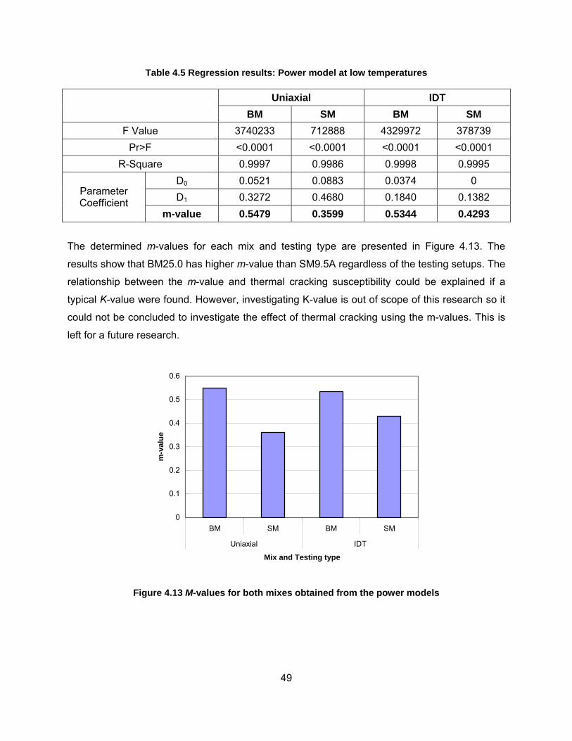
49

Table 4.5 Regression results: Power model at low temperatures

Uniaxial IDT

BM SM BM SM F Value 3740233 712888 4329972 378739

Pr>F <0.0001 <0.0001 <0.0001 <0.0001 R-Square 0.9997 0.9986 0.9998 0.9995

D0 0.0521 0.0883 0.0374 0 D1 0.3272 0.4680 0.1840 0.1382 Parameter

Coefficient m-value 0.5479 0.3599 0.5344 0.4293

The determined m-values for each mix and testing type are presented in Figure 4.13. The

results show that BM25.0 has higher m-value than SM9.5A regardless of the testing setups. The

relationship between the m-value and thermal cracking susceptibility could be explained if a

typical K-value were found. However, investigating K-value is out of scope of this research so it

could not be concluded to investigate the effect of thermal cracking using the m-values. This is

left for a future research.

0

0.1

0.2

0.3

0.4

0.5

0.6

BM SM BM SM

Uniaxial IDT

Mix and Testing type

m-v

alue

Figure 4.13 M-values for both mixes obtained from the power models

50

4.4. Summary

Creep compliance data of different asphalt mixtures were determined from creep test at five

temperatures (-15, 5, 20, 30, and 40°C) with different testing setups: uniaxial compressive and

indirect tension. Using the time-temperature superposition principle, the creep compliance curve

at each temperature was shifted to a reference temperature (20°C) to make a single smooth

line: the creep compliance master curve (CCMC). Shifting factors for each asphalt mixture were

visually determined with the aid of the Goal Seek function of the EXCEL spreadsheet.

Three mathematical models (the Prony series, sigmoidal, and power) were fitted to the CCMC

data using regression analysis. The result indicated that the sigmoidal model was the one that

best fit the data over the entire range of reduced times considered.

The susceptibility of mixes to thermal cracking was investigated using the m-value determined

at low temperatures. The BM25.0 has higher m-values than SM9.5A; however, a decision

regarding which mix is more susceptible to thermal cracking at low temperatures using m-value

could not be made.

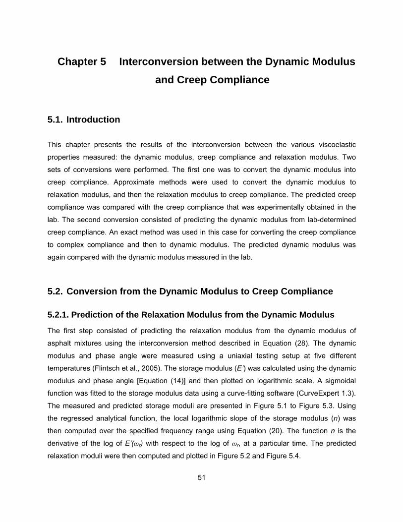
51

Chapter 5 Interconversion between the Dynamic Modulus and Creep Compliance

5.1. Introduction

This chapter presents the results of the interconversion between the various viscoelastic

properties measured: the dynamic modulus, creep compliance and relaxation modulus. Two

sets of conversions were performed. The first one was to convert the dynamic modulus into

creep compliance. Approximate methods were used to convert the dynamic modulus to

relaxation modulus, and then the relaxation modulus to creep compliance. The predicted creep

compliance was compared with the creep compliance that was experimentally obtained in the

lab. The second conversion consisted of predicting the dynamic modulus from lab-determined

creep compliance. An exact method was used in this case for converting the creep compliance

to complex compliance and then to dynamic modulus. The predicted dynamic modulus was

again compared with the dynamic modulus measured in the lab.

5.2. Conversion from the Dynamic Modulus to Creep Compliance

5.2.1. Prediction of the Relaxation Modulus from the Dynamic Modulus

The first step consisted of predicting the relaxation modulus from the dynamic modulus of

asphalt mixtures using the interconversion method described in Equation (28). The dynamic

modulus and phase angle were measured using a uniaxial testing setup at five different

temperatures (Flintsch et al., 2005). The storage modulus (E’) was calculated using the dynamic

modulus and phase angle [Equation (14)] and then plotted on logarithmic scale. A sigmoidal

function was fitted to the storage modulus data using a curve-fitting software (CurveExpert 1.3).

The measured and predicted storage moduli are presented in Figure 5.1 to Figure 5.3. Using

the regressed analytical function, the local logarithmic slope of the storage modulus (n) was

then computed over the specified frequency range using Equation (20). The function n is the

derivative of the log of E’(ωr) with respect to the log of ωr, at a particular time. The predicted

relaxation moduli were then computed and plotted in Figure 5.2 and Figure 5.4.

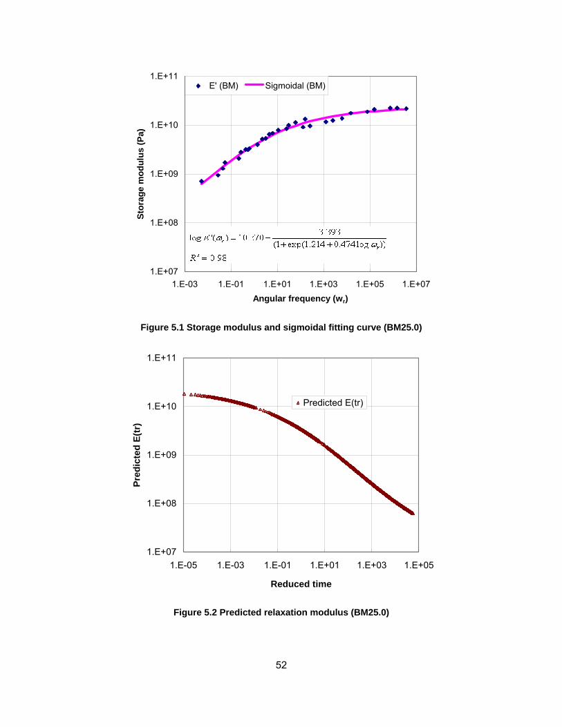
52

1.E+07

1.E+08

1.E+09

1.E+10

1.E+11

1.E-03 1.E-01 1.E+01 1.E+03 1.E+05 1.E+07Angular frequency (wr)

Stor

age

mod

ulus

(Pa)

E' (BM) Sigmoidal (BM)

Figure 5.1 Storage modulus and sigmoidal fitting curve (BM25.0)

1.E+07

1.E+08

1.E+09

1.E+10

1.E+11

1.E-05 1.E-03 1.E-01 1.E+01 1.E+03 1.E+05

Reduced time

Pred

icte

d E(

tr)

Predicted E(tr)

Figure 5.2 Predicted relaxation modulus (BM25.0)

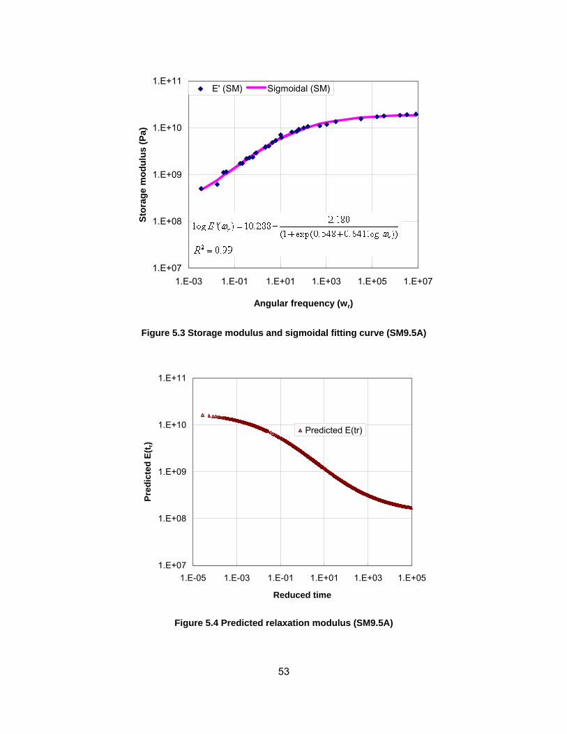
53

1.E+07

1.E+08

1.E+09

1.E+10

1.E+11

1.E-03 1.E-01 1.E+01 1.E+03 1.E+05 1.E+07

Angular frequency (wr)

Stor

age

mod

ulus

(Pa)

E' (SM) Sigmoidal (SM)

Figure 5.3 Storage modulus and sigmoidal fitting curve (SM9.5A)

1.E+07

1.E+08

1.E+09

1.E+10

1.E+11

1.E-05 1.E-03 1.E-01 1.E+01 1.E+03 1.E+05

Reduced time

Pred

icte

d E(

t r)

Predicted E(tr)

Figure 5.4 Predicted relaxation modulus (SM9.5A)

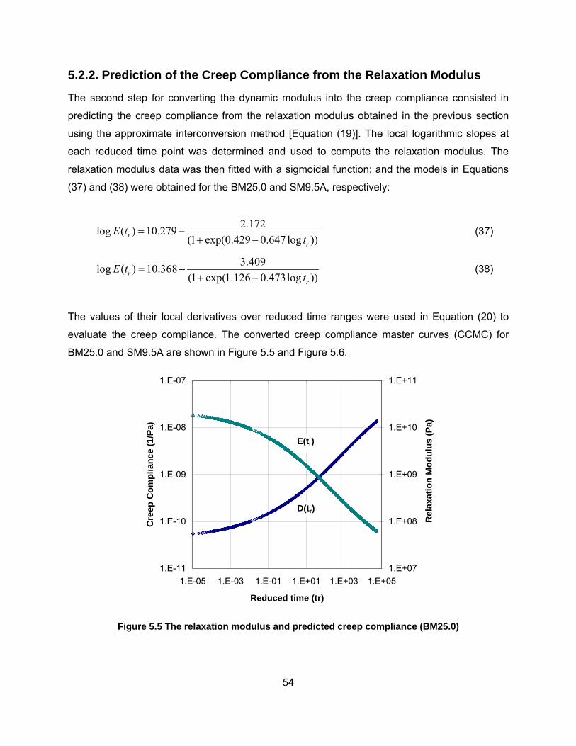
54

5.2.2. Prediction of the Creep Compliance from the Relaxation Modulus

The second step for converting the dynamic modulus into the creep compliance consisted in

predicting the creep compliance from the relaxation modulus obtained in the previous section

using the approximate interconversion method [Equation (19)]. The local logarithmic slopes at

each reduced time point was determined and used to compute the relaxation modulus. The

relaxation modulus data was then fitted with a sigmoidal function; and the models in Equations

(37) and (38) were obtained for the BM25.0 and SM9.5A, respectively:

2.172log ( ) 10.279(1 exp(0.429 0.647 log ))r

r

E tt

= −+ −

(37)

3.409log ( ) 10.368(1 exp(1.126 0.473log ))r

r

E tt

= −+ −

(38)

The values of their local derivatives over reduced time ranges were used in Equation (20) to

evaluate the creep compliance. The converted creep compliance master curves (CCMC) for

BM25.0 and SM9.5A are shown in Figure 5.5 and Figure 5.6.

1.E-11

1.E-10

1.E-09

1.E-08

1.E-07

1.E-05 1.E-03 1.E-01 1.E+01 1.E+03 1.E+05

Reduced time (tr)

Cre

ep C

ompl

ianc

e (1

/Pa)

1.E+07

1.E+08

1.E+09

1.E+10

1.E+11

Rel

axat

ion

Mod

ulus

(Pa)

D(tr)

E(tr)

Figure 5.5 The relaxation modulus and predicted creep compliance (BM25.0)

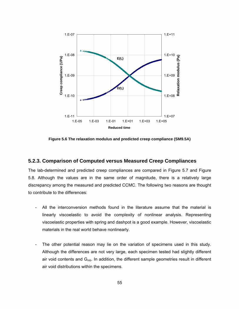
55

1.E-11

1.E-10

1.E-09

1.E-08

1.E-07

1.E-05 1.E-03 1.E-01 1.E+01 1.E+03 1.E+05

Reduced time

Cre

ep c

ompl

ianc

e (1

/Pa)

1.E+07

1.E+08

1.E+09

1.E+10

1.E+11

Rel

axat

ion

mod

ulus

(Pa)E(tr)

D(tr)

Figure 5.6 The relaxation modulus and predicted creep compliance (SM9.5A)

5.2.3. Comparison of Computed versus Measured Creep Compliances

The lab-determined and predicted creep compliances are compared in Figure 5.7 and Figure

5.8. Although the values are in the same order of magnitude, there is a relatively large

discrepancy among the measured and predicted CCMC. The following two reasons are thought

to contribute to the differences:

- All the interconversion methods found in the literature assume that the material is

linearly viscoelastic to avoid the complexity of nonlinear analysis. Representing

viscoelastic properties with spring and dashpot is a good example. However, viscoelastic

materials in the real world behave nonlinearly.

- The other potential reason may lie on the variation of specimens used in this study.

Although the differences are not very large, each specimen tested had slightly different

air void contents and Gmb. In addition, the different sample geometries result in different

air void distributions within the specimens.

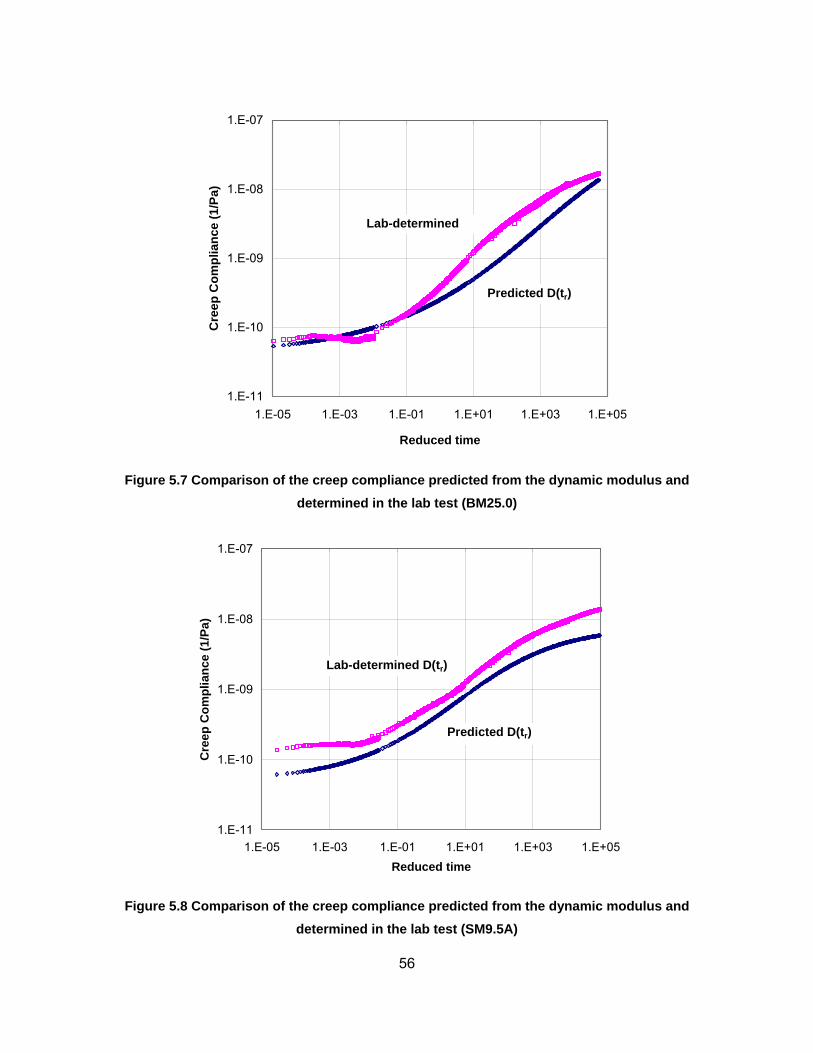
56

1.E-11

1.E-10

1.E-09

1.E-08

1.E-07

1.E-05 1.E-03 1.E-01 1.E+01 1.E+03 1.E+05

Reduced time

Cre

ep C

ompl

ianc

e (1

/Pa)

Predicted D(tr)

Lab-determined

Figure 5.7 Comparison of the creep compliance predicted from the dynamic modulus and determined in the lab test (BM25.0)

1.E-11

1.E-10

1.E-09

1.E-08

1.E-07

1.E-05 1.E-03 1.E-01 1.E+01 1.E+03 1.E+05Reduced time

Cre

ep C

ompl

ianc

e (1

/Pa)

Lab-determined D(tr)

Predicted D(tr)

Figure 5.8 Comparison of the creep compliance predicted from the dynamic modulus and determined in the lab test (SM9.5A)

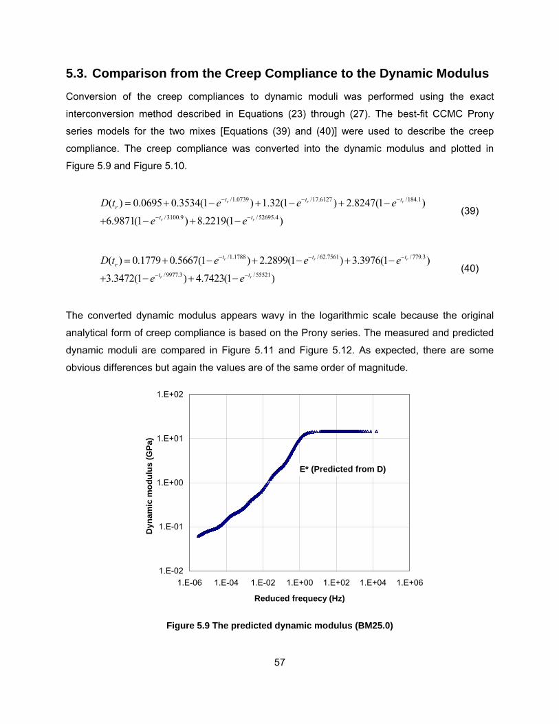
57

5.3. Comparison from the Creep Compliance to the Dynamic Modulus

Conversion of the creep compliances to dynamic moduli was performed using the exact

interconversion method described in Equations (23) through (27). The best-fit CCMC Prony

series models for the two mixes [Equations (39) and (40)] were used to describe the creep

compliance. The creep compliance was converted into the dynamic modulus and plotted in

Figure 5.9 and Figure 5.10.

/1.0739 /17.6127 /184.1

/3100.9 /52695.4

( ) 0.0695 0.3534(1 ) 1.32(1 ) 2.8247(1 )

6.9871(1 ) 8.2219(1 )

r r r

r r

t t tr

t t

D t e e e

e e

− − −

− −

= + − + − + −

+ − + − (39)

/1.1788 /62.7561 /779.3

/9977.3 /55521

( ) 0.1779 0.5667(1 ) 2.2899(1 ) 3.3976(1 )

3.3472(1 ) 4.7423(1 )

r r r

r r

t t tr

t t

D t e e e

e e

− − −

− −

= + − + − + −

+ − + − (40)

The converted dynamic modulus appears wavy in the logarithmic scale because the original

analytical form of creep compliance is based on the Prony series. The measured and predicted

dynamic moduli are compared in Figure 5.11 and Figure 5.12. As expected, there are some

obvious differences but again the values are of the same order of magnitude.

1.E-02

1.E-01

1.E+00

1.E+01

1.E+02

1.E-06 1.E-04 1.E-02 1.E+00 1.E+02 1.E+04 1.E+06

Reduced frequecy (Hz)

Dyn

amic

mod

ulus

(GPa

)

E* (Predicted from D)

Figure 5.9 The predicted dynamic modulus (BM25.0)

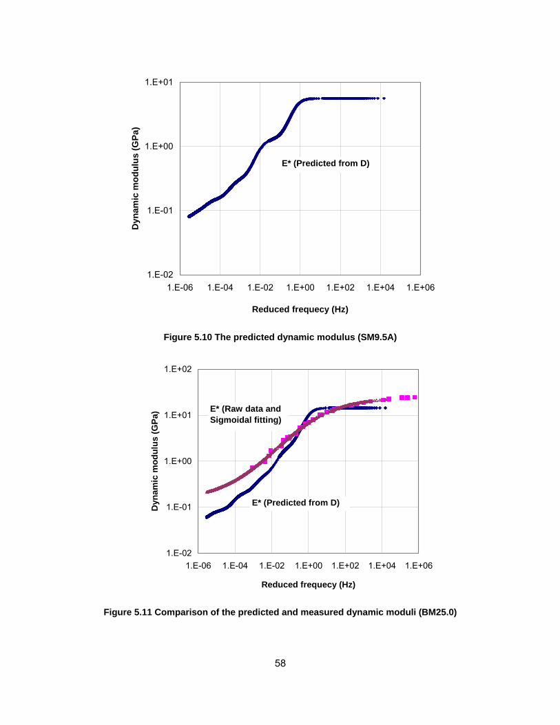
58

1.E-02

1.E-01

1.E+00

1.E+01

1.E-06 1.E-04 1.E-02 1.E+00 1.E+02 1.E+04 1.E+06

Reduced frequecy (Hz)

Dyn

amic

mod

ulus

(GPa

)

E* (Predicted from D)

Figure 5.10 The predicted dynamic modulus (SM9.5A)

1.E-02

1.E-01

1.E+00

1.E+01

1.E+02

1.E-06 1.E-04 1.E-02 1.E+00 1.E+02 1.E+04 1.E+06

Reduced frequecy (Hz)

Dyn

amic

mod

ulus

(GPa

)

E* (Predicted from D)

E* (Raw data and Sigmoidal fitting)

Figure 5.11 Comparison of the predicted and measured dynamic moduli (BM25.0)

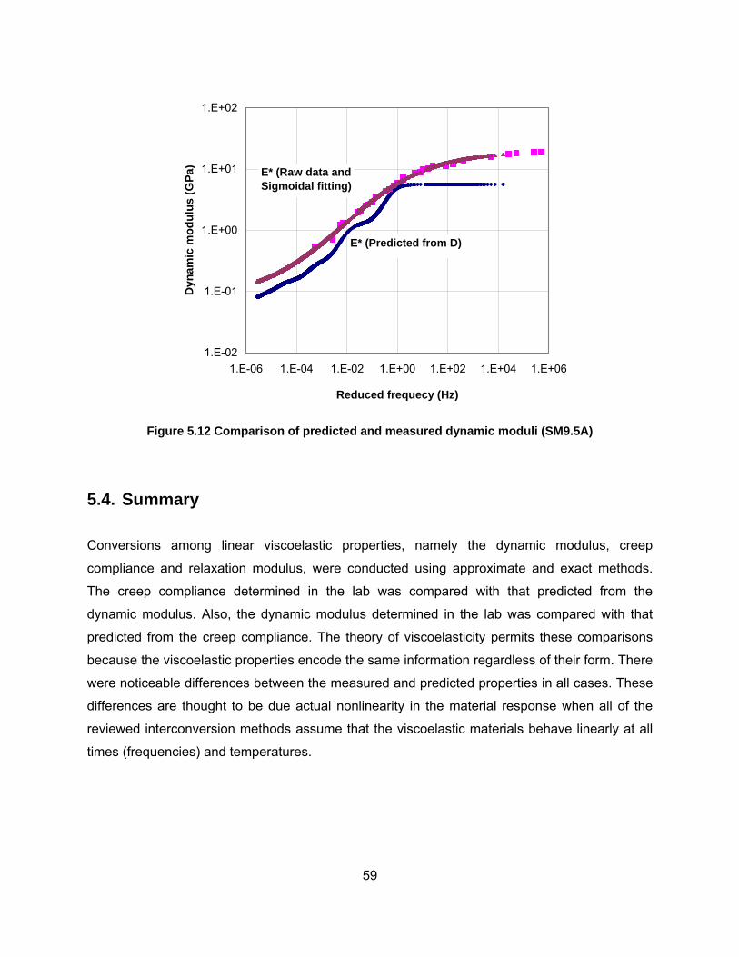
59

1.E-02

1.E-01

1.E+00

1.E+01

1.E+02

1.E-06 1.E-04 1.E-02 1.E+00 1.E+02 1.E+04 1.E+06

Reduced frequecy (Hz)

Dyn

amic

mod

ulus

(GPa

)

E* (Predicted from D)

E* (Raw data and Sigmoidal fitting)

Figure 5.12 Comparison of predicted and measured dynamic moduli (SM9.5A)

5.4. Summary

Conversions among linear viscoelastic properties, namely the dynamic modulus, creep

compliance and relaxation modulus, were conducted using approximate and exact methods.

The creep compliance determined in the lab was compared with that predicted from the

dynamic modulus. Also, the dynamic modulus determined in the lab was compared with that

predicted from the creep compliance. The theory of viscoelasticity permits these comparisons

because the viscoelastic properties encode the same information regardless of their form. There

were noticeable differences between the measured and predicted properties in all cases. These

differences are thought to be due actual nonlinearity in the material response when all of the

reviewed interconversion methods assume that the viscoelastic materials behave linearly at all

times (frequencies) and temperatures.

60

Chapter 6 Findings, Conclusions, and Recommendations

The creep compliance of two HMA mixes were measured in different testing setups (uniaxial

compressive and indirect tensile setups) and at various temperatures. Creep compliance master

curves (CCMCs) were constructed using the time-temperature superposition and modeled using

three mathematical functions: the Prony series, power, and sigmoidal. The SAS statistical

package was used to find the best-fit model for each mix and testing configuration and the

obtained models were investigated and compared. Using the m-value obtained from the power

model, the susceptibility to thermal cracking at low temperatures of the mixes was evaluated.

Finally, CCMC obtained from the dynamic modulus test and interconversion procedures were

compared with the CCMC determined experimentally using the uniaxial setup.

6.1. Findings

Several findings regarding creep compliance measurement and its application were produced in

this research. The main findings are summarized below:

• Creep compliance measurements at low temperatures were noisier than at high

temperatures. This was probably because the magnitude of the measurements approaches

the sensitivity of the measurement gauges. Furthermore, creep measurements with the IDT

setup were noisier, probably because the testing geometry, stress/strain distribution, and

method to calculate creep compliance are more complex in this configuration.

• The compliance data determined using the two testing setups were noticeably different. At

low temperatures, the uniaxial compressive creep was higher than that measured in the IDT

mode. This is consistent with previous findings. At higher temperatures the relationship

appears to be mix-dependent.

• To construct a more reliable master curve, the testing temperatures should be adjusted

especially between -15 and 5°C. The temperatures chosen for the investigation did not

produce enough overlap between the low temperature shifted curves. More overlap between

curves obtained at adjacent temperatures would increase the reliability of the master curve.

61

• The regression analysis conducted to fit the CCMC data indicate that the three

mathematical functions considered are appropriate to model the CCMC. The sigmoidal

function produced the best fit over the entire range of reduced times investigated for both

testing setups.

• Of the various Prony terms investigated, the five-term Prony series proved to be the most

appropriate for modeling the experimental CCMC data. However, the fitting was not very

good at low temperatures, probably because the least-square fitting was conducted in the

arithmetic scale (instead of using a logarithmic transformation).

• The m-values for BM25.0 were higher than those for SM9.5A regardless of the testing setup

used to measure the creep compliance.

• The dynamic modulus determined in a uniaxial setup was successfully converted into creep

compliance with the same setup. However, although they were in the same order of

magnitude the predicted and measured values are noticeably different. This is thought to be

due to nonlinear behavior of viscoelastic material. The sigmoidal function performed better

than the Prony series when used in the interconversion procedure because of the Prony

series model was too wavy.

6.2. Conclusions

The results of the experimental program conducted support the conclusion that the three

mathematical models considered (the Prony series, power and sigmoidal) are appropriate to

model the CCMC over a wide range of reduced times. However, the sigmoidal model produced

the best fit over the entire range investigated. This model also produced the best results when

used in the interconversion procedures. A noticeable difference was observed between the

CCMC predicted from dynamic modulus measurements and those obtained experimentally, this

is probably because the interconversion method is based on the assumption that the material

displays linear viscoelasticity.

6.3. Recommendations

Based on the results of this study, the following recommendations can be made to improve the

development of the CCMC and to obtain a stronger conclusion in future investigations.

62

• The set of testing temperatures should be revised to produce more overlap between the

shifted adjacent curves. This would allow the development of more reliable shifting, and

consequently better CCMC. Temperature increments of less than 10°C over the entire

range of temperatures are recommended.

• The sigmoidal function should be used to model the CCMC of HMA over a large range of

reduced times. The power model produces good results at low temperatures and should

continue to be used to assess the susceptibility of HMA to thermal cracking.

• The conversion of the creep compliance into the dynamic modulus and vice versa

appears to work better when using a sigmoidal function than when using the Prony

series recommended in the literature. The sigmoidal function produces a smoother

CCMC. Furthermore, it may be necessary to shift the converted CCMC to account for

nonlinearity in the behavior of the HMA. More mixes should be investigated to assess

the feasibility of defining correction shift factors.

63

References

AASHTO T332-03. Determining the Creep Compliance and Strength of Hot Mix Asphalt (HMA) Using the Indirect Tensile Test Device. American Association of State Highway and Transportation Officials, 25th edition, 2005. Brown, E.R. and K.Y. Foo, “Comparison of Unconfined- and Confined-Creep Tests for Hot Mix Asphalt,” Journal of Materials in Civil Engineering, Vol. 6, No. 2, pp. 307-326, May, 1994. Buttlar, W.G. and R. Roque, “Development and Evaluation of the Strategic Highway Research Program Measurement and Analysis System for Indirect Testing at Low Temperatures,” Transportation Research Record No.1454, Transportation Research Board, Washington, D.C., pp. 163-171, 1994. Christensen, D.W. and R.F. Bonaquist, “Evaluation of Indirect Tensile Test (IDT) Procedures for Low-Temperature Performance of Hot Mix Asphalt,” NCHRP Report 530, Transportation Research Board, Washington DC, 2004. Christison, J.T., D.W. Murray and K.O. Anderson, “Stress Prediction and Low Temperature Fracture Susceptibility of Asphaltic Concrete Pavements,” Journal of the Association of Asphalt Paving Technologist, Vol. 41, pp. 494-523, 1972. Ferry, J.D., Viscoelastic properties of polymers, 3rd ed., Wiley, New York, 1980. Finn, F., C.L. Saraf, R. Kulkarni, K. Nair, W. Smith, and A. Abdullah, “Development of Pavement Subsystems,” NCHRP Report 291, Transportation Research Board, Washington DC, 1986. Flintsch, G.W., I.L. Al-Qadi, A. Loulizi, and D. Mokarem, “Laboratory Tests for Hot-Mix Asphalt Characterization in Virginia,” VTRC Report 05-CR22, Charlottesville, VA, 2005. Fromm, H.J. and W.A. Phang, “A Study of Transverse Cracking of Bituminous Pavements,” Proceedings, Association of Asphalt Paving Technologists, Vol. 41, pp. 383-423, 1972. Hafez, I. “Development of a Simplified Asphalt Mix Stability Procedure for Use in Superpave Volumetric Mix Design,” Ph.D. Dissertation, Civil Engineering Department, University of Maryland, College Park, MD, 1997. Hass, R., F. Meyer, G. Assaf, and H. Lee, “A Comprehensive Study of Cold Climate Airport Pavement Cracking,” Proceedings, Association of Asphalt Paving Technologists, Vol. 56, pp. 198-245, 1987. Hills, J.F. and D. Brien, “The Fracture of Bitumens and Asphalt Mixes by Temperature Induced Stresses,” Prepared Discussion, Proceedings, Association of Asphalt Paving Technologists, Vol. 35, pp. 292-309, 1966

64

Hiltunen, D.R. and R. Roque, “A Mechanics-Based Prediction Model for Thermal Cracking of Asphaltic Concrete Pavements,” Journal of the Association of Asphalt Paving Technologists, Vol. 63, pp. 81-117, 1994. Hiltunen, D.R. and R. Roque, “The Use of Time-Temperature Superposition to Fundamentally Characterize Asphaltic Concrete Mixtures at Low Temperatures,” Engineering Properties of Asphalt Mixtures and the Relationship to their Performance, ASTM STP 1265, Gerald A. Huber and Dale S. Decker, Eds., American Society for Testing and Materials, Philadelphia, 1995. Huang, Y.H., Pavement Analysis and Design, Englewood Cliffs, N.J.: Prentice-Hall, Inc., 1993. InstroTek Inc., CoreLok Operators Guide, 2003. Kim, Y.R., J.S. Daniel and H. Wen, “Fatigue Evaluation of WesTrack Asphalt Mixtures Using Viscoelastic Continuum Damage Approach,” Final Report, North Carolina Department of Transportation, Research Project No. HWY-0678, Raleigh, NC, 2002. Leaderman, H., “Viscoelasticity phenomena in amorphous high polymeric systems,” Rheology, Vol. II, F.R. Eirich, ed., Academic, New York, 1958. Lakes, R. S., Viscoelastic Solids, Boca Raton, FL: CRC Press LLC, 1999.

Lytton, R.L., U. Shanmugham and B.D. Garrett, “Design of Asphalt Pavements for Thermal Fatigue Cracking,” Research Report 284-4, Texas Transportation Institute, 1983. McLeod, N.W., “A 4-year Survey of Low-Temperature Transverse Pavement Cracking on Three Ontario Test-Roads,” Proceedings, Association of Asphalt Paving Technologists, Vol. 41, 1972. Molenaar, A.A.A., Structural Performance and Design of Flexible Road Constructions and Asphalt Concrete Overlays, Ph.D. Dissertation, Delft University of Technology, Netherlands, 1983. Painter, P.C. and M.M. Coleman, Fundamentals of Polymer Science – An Introductory Text, Technomic Publishing Co.Inc., ISBN 1-56676-559-5, Lancaster, PA, 1997. Paris, P.C. and F. Erdogan, “A Critical Analysis of Crack Propagation Laws,” Transactions of the ASME, Journal of Basic Engineering, Series D, 85, No. 3, 1963. Park, S.W. and R.A. Schapery, “Methods of interconversion between linear viscoelastic material functions. Part I-a numerical method based on Prony series,” International Journal of Solids and Structures, Vol. 36, pp. 1653-1675, 1999. Park, S.W. and Y.R. Kim, “Interconversion between Relaxation Modulus and Creep Compliance for Viscoelastic Solids,” ASCE Journal of Materials in Civil Engineering, Vol. 11, No. 1, pp. 76-82, 1999. Park, S.W. and Y.R. Kim, “Fitting Prony-Series Viscoelastic Models with Power-Law Pre-Smoothing,” ASCE Journal of Materials in Civil Engineering, Vol. 13, No. 1, pp.26-32, 2001.

65

Pellinen, T.K. and M.W. Witczak, “Stress Dependent Master Curve Construction for Dynamic (Complex) Modulus,” Journal of the Association of Asphalt Paving Technologists, Vol. 71, 2004. Roque, R., D.H. Hiltunen, W.G. Buttlar, and T. Farwana, “Development of the SHRP Superpave Mixture Specification Test Method to Control Thermal Cracking Performance of Pavements,” Engineering Properties of Asphalt Mixtures and the Relationship to their Performance, ASTM STP 1265, Gerald A. Huber and Dale S. Decker, Eds., American Society for Testing and Materials, Philadelphia, 1995. Schapery, R.A. and S.W. Park, “Methods of interconversion between linear viscoelastic material functions. Part II-an approximate analytical method,” International Journal of Solids and Structures, Vol. 36, pp. 1677-1699, 1999. Witczak, M.W., R. Roque, D.R. Hiltunen, and W.G. Buttlar, “Modification and Re-Calibration of Superpave Thermal Cracking Model,” NCHRP 9-19 Project Report, Arizona State University Department of Civil and Environmental Engineering, Tempe, Arizona, December 2000. Witczak, M.W., K. Kaloush, T.K. Pellinen, M. El-Basyouny, and H. Von Quitus, “Simple Performance Test for Superpave Mix Design,” NCHRP Report 465, Transportation Research Board, Washington DC, 2002.

66

Appendix A: Fitting model SAS Input and Output

67

A.1 Prony series model

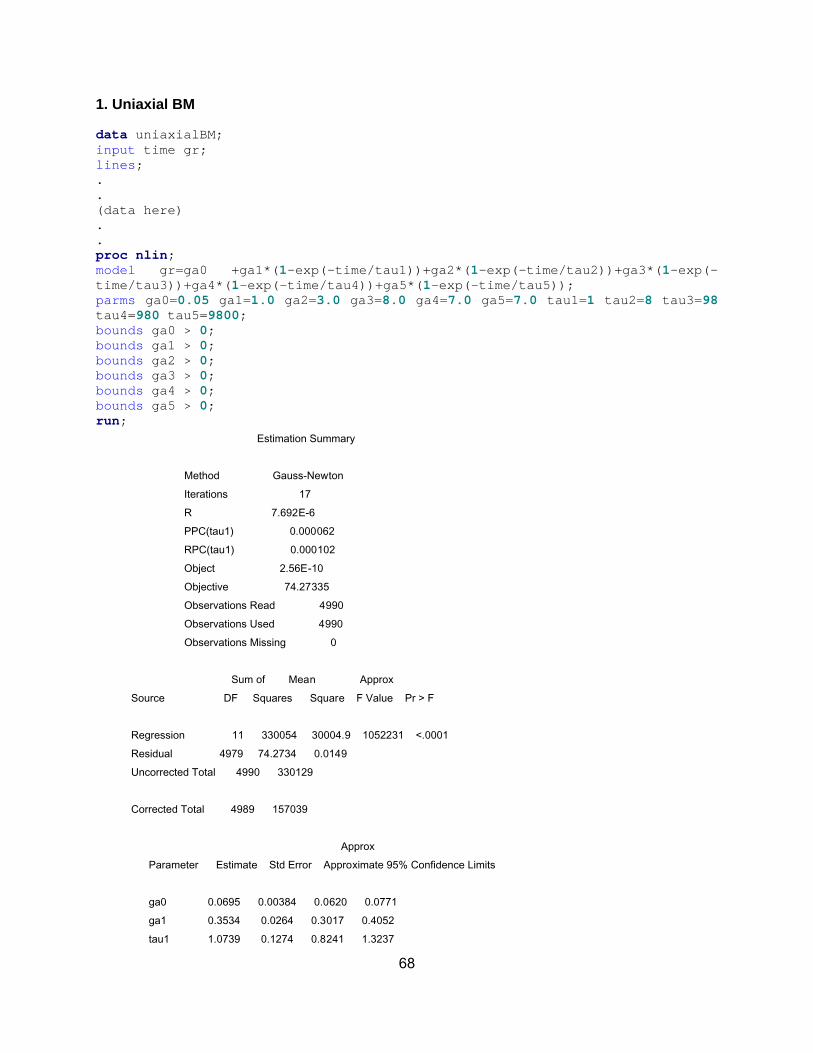
68

1. Uniaxial BM data uniaxialBM; input time gr; lines; . . (data here) . . proc nlin; model gr=ga0 +ga1*(1-exp(-time/tau1))+ga2*(1-exp(-time/tau2))+ga3*(1-exp(-time/tau3))+ga4*(1-exp(-time/tau4))+ga5*(1-exp(-time/tau5)); parms ga0=0.05 ga1=1.0 ga2=3.0 ga3=8.0 ga4=7.0 ga5=7.0 tau1=1 tau2=8 tau3=98 tau4=980 tau5=9800; bounds ga0 > 0; bounds ga1 > 0; bounds ga2 > 0; bounds ga3 > 0; bounds ga4 > 0; bounds ga5 > 0; run; Estimation Summary Method Gauss-Newton Iterations 17 R 7.692E-6 PPC(tau1) 0.000062 RPC(tau1) 0.000102 Object 2.56E-10 Objective 74.27335 Observations Read 4990 Observations Used 4990 Observations Missing 0 Sum of Mean Approx Source DF Squares Square F Value Pr > F Regression 11 330054 30004.9 1052231 <.0001 Residual 4979 74.2734 0.0149 Uncorrected Total 4990 330129 Corrected Total 4989 157039 Approx Parameter Estimate Std Error Approximate 95% Confidence Limits ga0 0.0695 0.00384 0.0620 0.0771 ga1 0.3534 0.0264 0.3017 0.4052 tau1 1.0739 0.1274 0.8241 1.3237

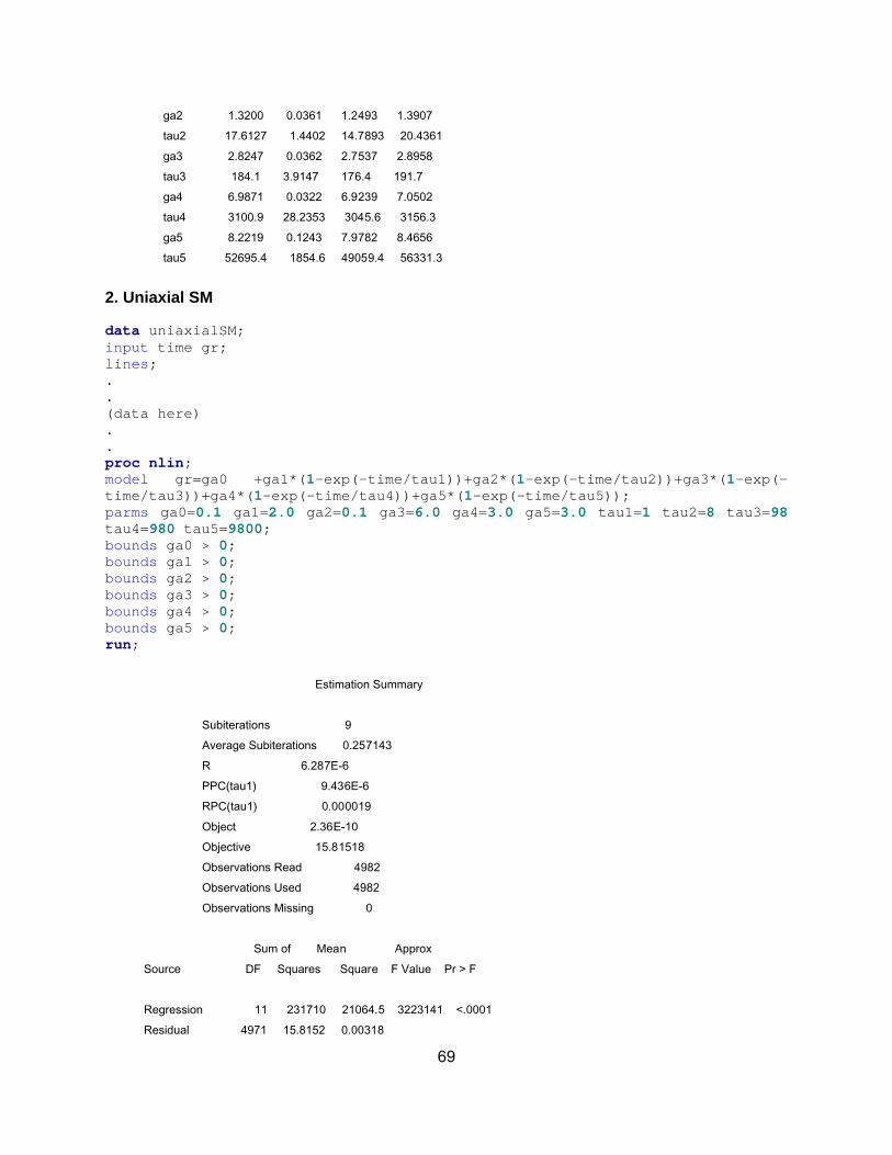
69

ga2 1.3200 0.0361 1.2493 1.3907 tau2 17.6127 1.4402 14.7893 20.4361 ga3 2.8247 0.0362 2.7537 2.8958 tau3 184.1 3.9147 176.4 191.7 ga4 6.9871 0.0322 6.9239 7.0502 tau4 3100.9 28.2353 3045.6 3156.3 ga5 8.2219 0.1243 7.9782 8.4656 tau5 52695.4 1854.6 49059.4 56331.3

2. Uniaxial SM data uniaxialSM; input time gr; lines; . . (data here) . . proc nlin; model gr=ga0 +ga1*(1-exp(-time/tau1))+ga2*(1-exp(-time/tau2))+ga3*(1-exp(-time/tau3))+ga4*(1-exp(-time/tau4))+ga5*(1-exp(-time/tau5)); parms ga0=0.1 ga1=2.0 ga2=0.1 ga3=6.0 ga4=3.0 ga5=3.0 tau1=1 tau2=8 tau3=98 tau4=980 tau5=9800; bounds ga0 > 0; bounds ga1 > 0; bounds ga2 > 0; bounds ga3 > 0; bounds ga4 > 0; bounds ga5 > 0; run;

Estimation Summary Subiterations 9 Average Subiterations 0.257143 R 6.287E-6 PPC(tau1) 9.436E-6 RPC(tau1) 0.000019 Object 2.36E-10 Objective 15.81518 Observations Read 4982 Observations Used 4982 Observations Missing 0 Sum of Mean Approx Source DF Squares Square F Value Pr > F Regression 11 231710 21064.5 3223141 <.0001 Residual 4971 15.8152 0.00318

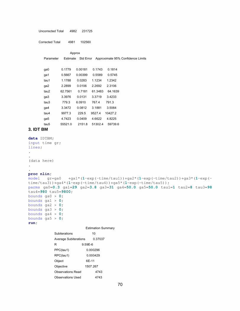
70

Uncorrected Total 4982 231725 Corrected Total 4981 102560 Approx Parameter Estimate Std Error Approximate 95% Confidence Limits ga0 0.1779 0.00181 0.1743 0.1814 ga1 0.5667 0.00399 0.5589 0.5745 tau1 1.1788 0.0283 1.1234 1.2342 ga2 2.2899 0.0106 2.2692 2.3106 tau2 62.7561 0.7181 61.3483 64.1639 ga3 3.3976 0.0131 3.3719 3.4233 tau3 779.3 6.0910 767.4 791.3 ga4 3.3472 0.0812 3.1881 3.5064 tau4 9977.3 229.5 9527.4 10427.2 ga5 4.7423 0.0409 4.6622 4.8225 tau5 55521.0 2151.8 51302.4 59739.6 3. IDT BM data IDTBM; input time gr; lines; . . (data here) . . proc nlin; model gr=ga0 +ga1*(1-exp(-time/tau1))+ga2*(1-exp(-time/tau2))+ga3*(1-exp(-time/tau3))+ga4*(1-exp(-time/tau4))+ga5*(1-exp(-time/tau5)); parms ga0=0.3 ga1=29 ga2=3.8 ga3=31 ga4=50.0 ga5=50.0 tau1=1 tau2=8 tau3=98 tau4=980 tau5=9800; bounds ga0 > 0; bounds ga1 > 0; bounds ga2 > 0; bounds ga3 > 0; bounds ga4 > 0; bounds ga5 > 0; run; Estimation Summary Subiterations 10 Average Subiterations 0.37037 R 9.59E-6 PPC(tau1) 0.000296 RPC(tau1) 0.000429 Object 6E-11 Objective 1507.267 Observations Read 4743 Observations Used 4743

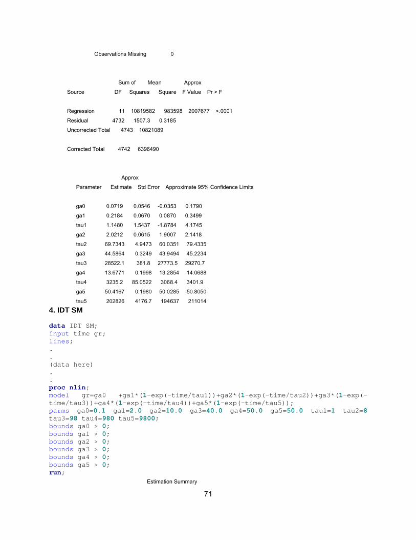
71

Observations Missing 0 Sum of Mean Approx Source DF Squares Square F Value Pr > F Regression 11 10819582 983598 2007677 <.0001 Residual 4732 1507.3 0.3185 Uncorrected Total 4743 10821089 Corrected Total 4742 6396490 Approx Parameter Estimate Std Error Approximate 95% Confidence Limits ga0 0.0719 0.0546 -0.0353 0.1790 ga1 0.2184 0.0670 0.0870 0.3499 tau1 1.1480 1.5437 -1.8784 4.1745 ga2 2.0212 0.0615 1.9007 2.1418 tau2 69.7343 4.9473 60.0351 79.4335 ga3 44.5864 0.3249 43.9494 45.2234 tau3 28522.1 381.8 27773.5 29270.7 ga4 13.6771 0.1998 13.2854 14.0688 tau4 3235.2 85.0522 3068.4 3401.9 ga5 50.4167 0.1980 50.0285 50.8050 tau5 202826 4176.7 194637 211014 4. IDT SM data IDT SM; input time gr; lines; . . (data here) . . proc nlin; model gr=ga0 +ga1*(1-exp(-time/tau1))+ga2*(1-exp(-time/tau2))+ga3*(1-exp(-time/tau3))+ga4*(1-exp(-time/tau4))+ga5*(1-exp(-time/tau5)); parms ga0=0.1 ga1=2.0 ga2=10.0 ga3=40.0 ga4=50.0 ga5=50.0 tau1=1 tau2=8 tau3=98 tau4=980 tau5=9800; bounds ga0 > 0; bounds ga1 > 0; bounds ga2 > 0; bounds ga3 > 0; bounds ga4 > 0; bounds ga5 > 0; run; Estimation Summary

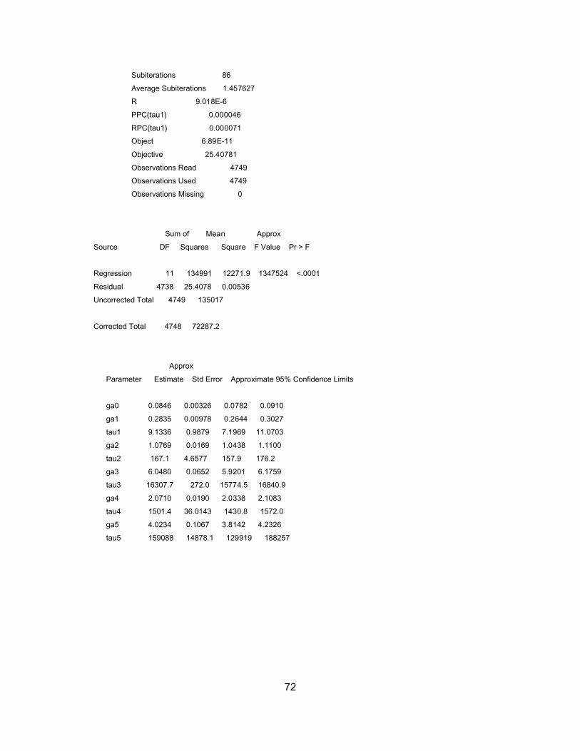
72

Subiterations 86 Average Subiterations 1.457627 R 9.018E-6 PPC(tau1) 0.000046 RPC(tau1) 0.000071 Object 6.89E-11 Objective 25.40781 Observations Read 4749 Observations Used 4749 Observations Missing 0 Sum of Mean Approx Source DF Squares Square F Value Pr > F Regression 11 134991 12271.9 1347524 <.0001 Residual 4738 25.4078 0.00536 Uncorrected Total 4749 135017 Corrected Total 4748 72287.2 Approx Parameter Estimate Std Error Approximate 95% Confidence Limits ga0 0.0846 0.00326 0.0782 0.0910 ga1 0.2835 0.00978 0.2644 0.3027 tau1 9.1336 0.9879 7.1969 11.0703 ga2 1.0769 0.0169 1.0438 1.1100 tau2 167.1 4.6577 157.9 176.2 ga3 6.0480 0.0652 5.9201 6.1759 tau3 16307.7 272.0 15774.5 16840.9 ga4 2.0710 0.0190 2.0338 2.1083 tau4 1501.4 36.0143 1430.8 1572.0 ga5 4.0234 0.1067 3.8142 4.2326 tau5 159088 14878.1 129919 188257

73

A.2 Power model

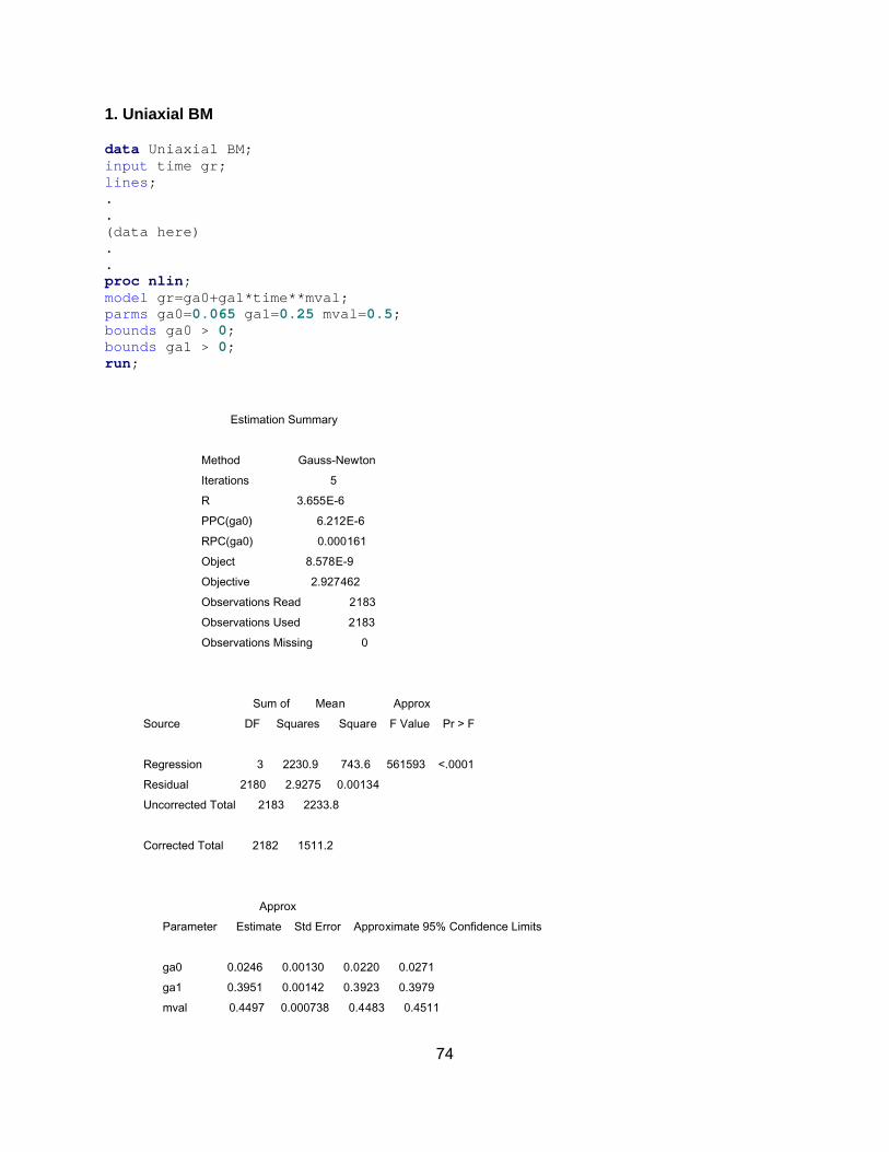
74

1. Uniaxial BM data Uniaxial BM; input time gr; lines; . . (data here) . . proc nlin; model gr=ga0+ga1*time**mval; parms ga0=0.065 ga1=0.25 mval=0.5; bounds ga0 > 0; bounds ga1 > 0; run; Estimation Summary Method Gauss-Newton Iterations 5 R 3.655E-6 PPC(ga0) 6.212E-6 RPC(ga0) 0.000161 Object 8.578E-9 Objective 2.927462 Observations Read 2183 Observations Used 2183 Observations Missing 0 Sum of Mean Approx Source DF Squares Square F Value Pr > F Regression 3 2230.9 743.6 561593 <.0001 Residual 2180 2.9275 0.00134 Uncorrected Total 2183 2233.8 Corrected Total 2182 1511.2 Approx Parameter Estimate Std Error Approximate 95% Confidence Limits ga0 0.0246 0.00130 0.0220 0.0271 ga1 0.3951 0.00142 0.3923 0.3979 mval 0.4497 0.000738 0.4483 0.4511

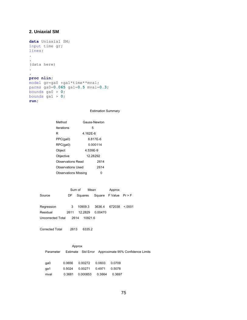
75

2. Uniaxial SM data Uniaxial SM; input time gr; lines; . . (data here) . . proc nlin; model gr=ga0 +ga1*time**mval; parms ga0=0.065 ga1=0.5 mval=0.3; bounds ga0 > 0; bounds ga1 > 0; run;

Estimation Summary Method Gauss-Newton Iterations 5 R 4.162E-6 PPC(ga0) 6.817E-6 RPC(ga0) 0.000114 Object 4.539E-9 Objective 12.28292 Observations Read 2614 Observations Used 2614 Observations Missing 0 Sum of Mean Approx Source DF Squares Square F Value Pr > F Regression 3 10909.3 3636.4 672038 <.0001 Residual 2611 12.2829 0.00470 Uncorrected Total 2614 10921.6 Corrected Total 2613 6335.2 Approx Parameter Estimate Std Error Approximate 95% Confidence Limits ga0 0.0656 0.00272 0.0603 0.0709 ga1 0.5024 0.00271 0.4971 0.5078 mval 0.3681 0.000853 0.3664 0.3697

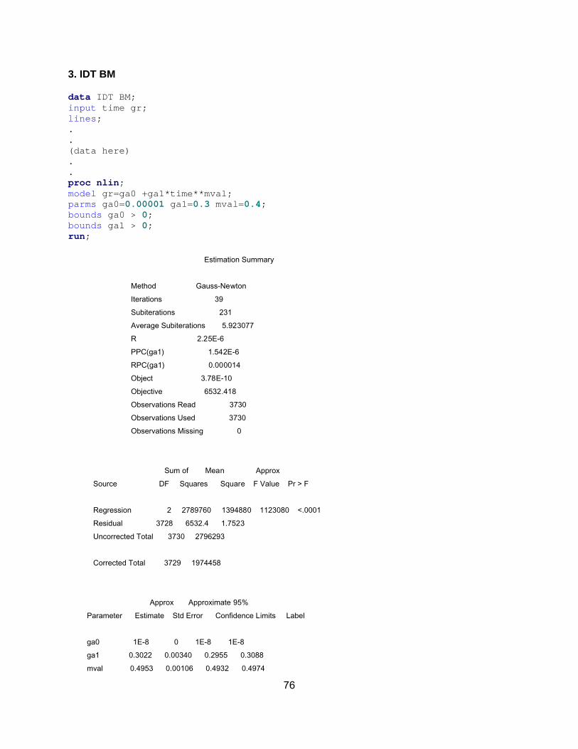
76

3. IDT BM data IDT BM; input time gr; lines; . . (data here) . . proc nlin; model gr=ga0 +ga1*time**mval; parms ga0=0.00001 ga1=0.3 mval=0.4; bounds ga0 > 0; bounds ga1 > 0; run;

Estimation Summary Method Gauss-Newton Iterations 39 Subiterations 231 Average Subiterations 5.923077 R 2.25E-6 PPC(ga1) 1.542E-6 RPC(ga1) 0.000014 Object 3.78E-10 Objective 6532.418 Observations Read 3730 Observations Used 3730 Observations Missing 0 Sum of Mean Approx Source DF Squares Square F Value Pr > F Regression 2 2789760 1394880 1123080 <.0001 Residual 3728 6532.4 1.7523 Uncorrected Total 3730 2796293 Corrected Total 3729 1974458 Approx Approximate 95% Parameter Estimate Std Error Confidence Limits Label ga0 1E-8 0 1E-8 1E-8 ga1 0.3022 0.00340 0.2955 0.3088 mval 0.4953 0.00106 0.4932 0.4974

77

Bound1 1081.1 49.8802 983.3 1178.8 0 < ga0

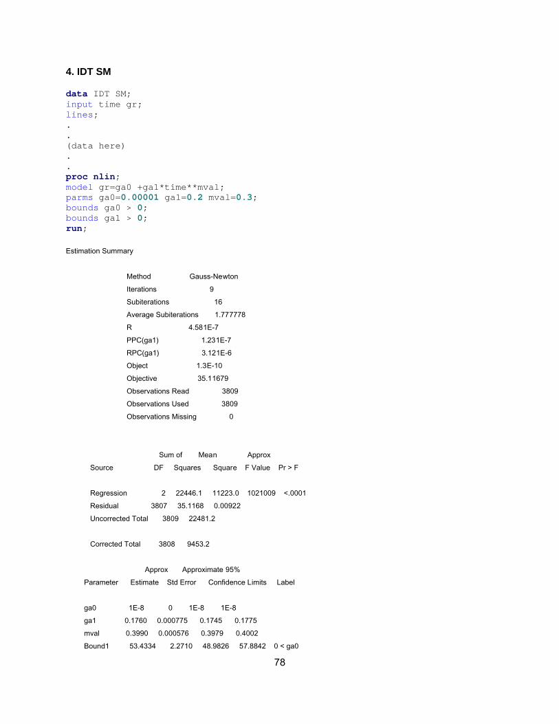
78

4. IDT SM data IDT SM; input time gr; lines; . . (data here) . . proc nlin; model gr=ga0 +ga1*time**mval; parms ga0=0.00001 ga1=0.2 mval=0.3; bounds ga0 > 0; bounds ga1 > 0; run; Estimation Summary Method Gauss-Newton Iterations 9 Subiterations 16 Average Subiterations 1.777778 R 4.581E-7 PPC(ga1) 1.231E-7 RPC(ga1) 3.121E-6 Object 1.3E-10 Objective 35.11679 Observations Read 3809 Observations Used 3809 Observations Missing 0 Sum of Mean Approx Source DF Squares Square F Value Pr > F Regression 2 22446.1 11223.0 1021009 <.0001 Residual 3807 35.1168 0.00922 Uncorrected Total 3809 22481.2 Corrected Total 3808 9453.2 Approx Approximate 95% Parameter Estimate Std Error Confidence Limits Label ga0 1E-8 0 1E-8 1E-8 ga1 0.1760 0.000775 0.1745 0.1775 mval 0.3990 0.000576 0.3979 0.4002 Bound1 53.4334 2.2710 48.9826 57.8842 0 < ga0

79

A.3 Sigmoidal model

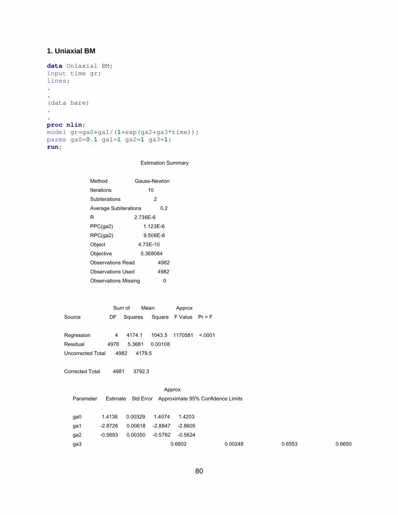
80

1. Uniaxial BM data Uniaxial BM; input time gr; lines; . . (data here) . . proc nlin; model gr=ga0+ga1/(1+exp(ga2+ga3*time)); parms ga0=0.1 ga1=1 ga2=1 ga3=1; run;

Estimation Summary Method Gauss-Newton Iterations 10 Subiterations 2 Average Subiterations 0.2 R 2.736E-6 PPC(ga2) 1.123E-6 RPC(ga2) 9.506E-6 Object 4.73E-10 Objective 5.368084 Observations Read 4982 Observations Used 4982 Observations Missing 0 Sum of Mean Approx Source DF Squares Square F Value Pr > F Regression 4 4174.1 1043.5 1170581 <.0001 Residual 4978 5.3681 0.00108 Uncorrected Total 4982 4179.5 Corrected Total 4981 3792.3

Approx Parameter Estimate Std Error Approximate 95% Confidence Limits ga0 1.4138 0.00329 1.4074 1.4203 ga1 -2.8726 0.00618 -2.8847 -2.8605 ga2 -0.5693 0.00350 -0.5762 -0.5624 ga3 0.6602 0.00248 0.6553 0.6650

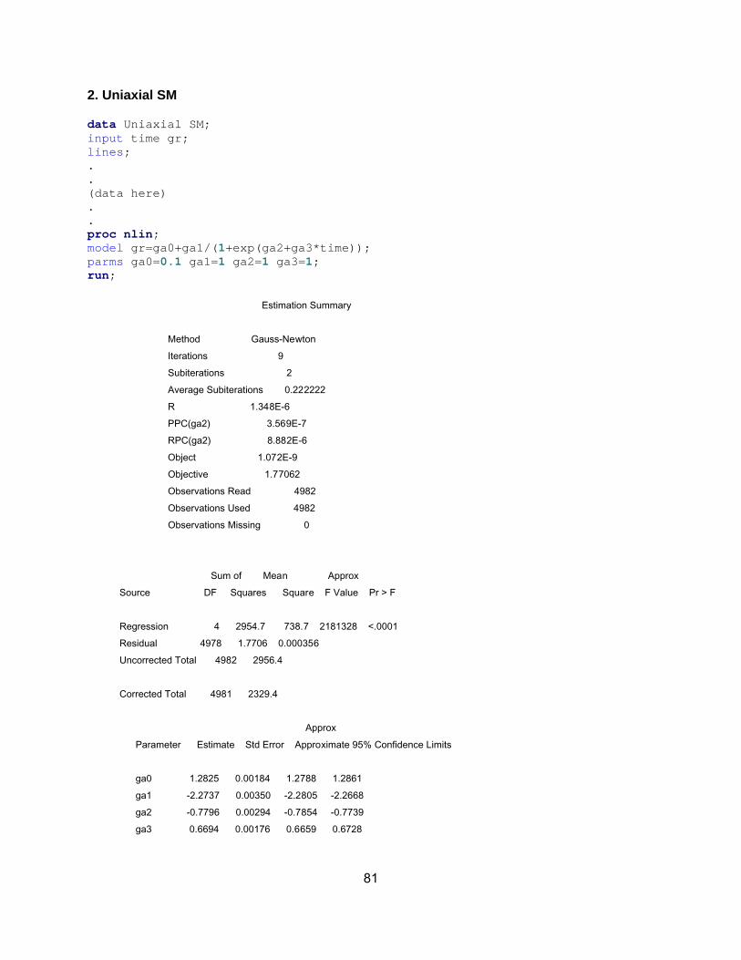
81

2. Uniaxial SM data Uniaxial SM; input time gr; lines; . . (data here) . . proc nlin; model gr=ga0+ga1/(1+exp(ga2+ga3*time)); parms ga0=0.1 ga1=1 ga2=1 ga3=1; run;

Estimation Summary Method Gauss-Newton Iterations 9 Subiterations 2 Average Subiterations 0.222222 R 1.348E-6 PPC(ga2) 3.569E-7 RPC(ga2) 8.882E-6 Object 1.072E-9 Objective 1.77062 Observations Read 4982 Observations Used 4982 Observations Missing 0 Sum of Mean Approx Source DF Squares Square F Value Pr > F Regression 4 2954.7 738.7 2181328 <.0001 Residual 4978 1.7706 0.000356 Uncorrected Total 4982 2956.4 Corrected Total 4981 2329.4

Approx Parameter Estimate Std Error Approximate 95% Confidence Limits ga0 1.2825 0.00184 1.2788 1.2861 ga1 -2.2737 0.00350 -2.2805 -2.2668 ga2 -0.7796 0.00294 -0.7854 -0.7739 ga3 0.6694 0.00176 0.6659 0.6728

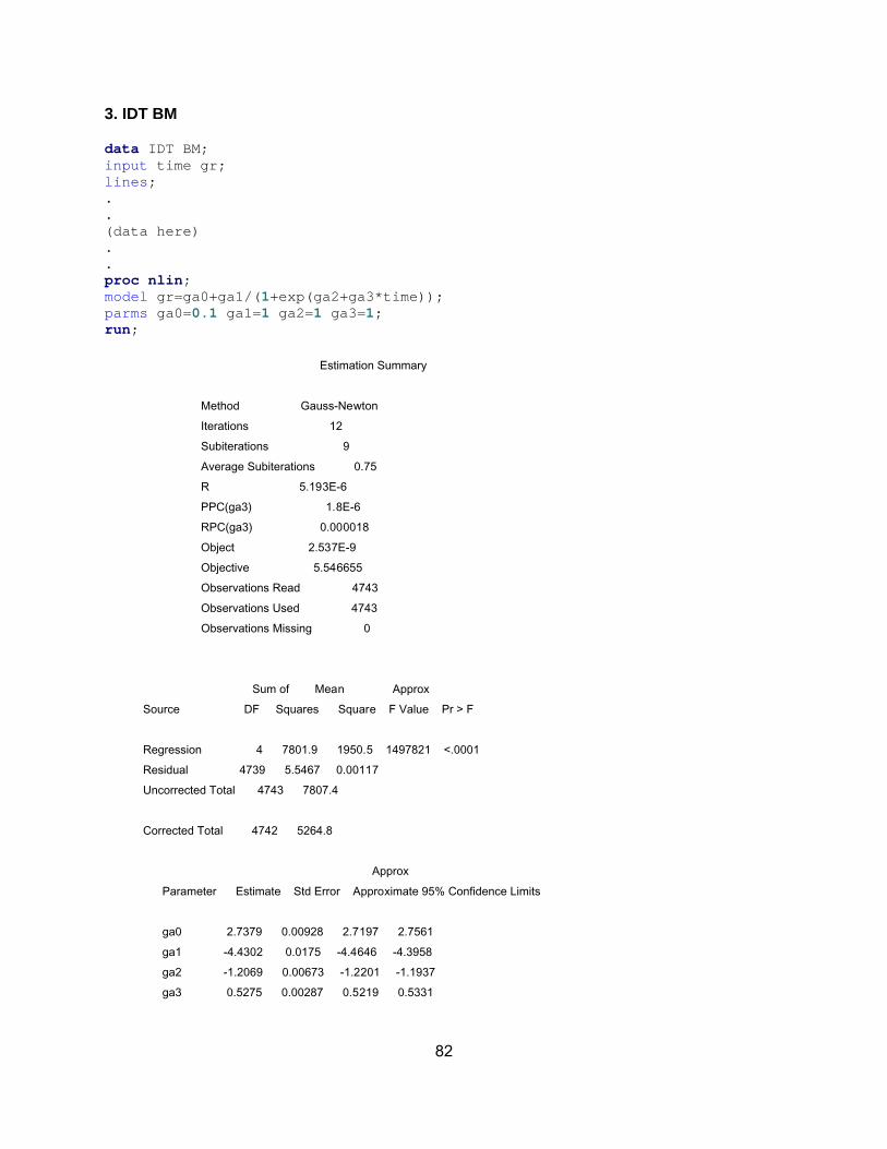
82

3. IDT BM data IDT BM; input time gr; lines; . . (data here) . . proc nlin; model gr=ga0+ga1/(1+exp(ga2+ga3*time)); parms ga0=0.1 ga1=1 ga2=1 ga3=1; run; Estimation Summary Method Gauss-Newton Iterations 12 Subiterations 9 Average Subiterations 0.75 R 5.193E-6 PPC(ga3) 1.8E-6 RPC(ga3) 0.000018 Object 2.537E-9 Objective 5.546655 Observations Read 4743 Observations Used 4743 Observations Missing 0 Sum of Mean Approx Source DF Squares Square F Value Pr > F Regression 4 7801.9 1950.5 1497821 <.0001 Residual 4739 5.5467 0.00117 Uncorrected Total 4743 7807.4 Corrected Total 4742 5264.8

Approx Parameter Estimate Std Error Approximate 95% Confidence Limits ga0 2.7379 0.00928 2.7197 2.7561 ga1 -4.4302 0.0175 -4.4646 -4.3958 ga2 -1.2069 0.00673 -1.2201 -1.1937 ga3 0.5275 0.00287 0.5219 0.5331

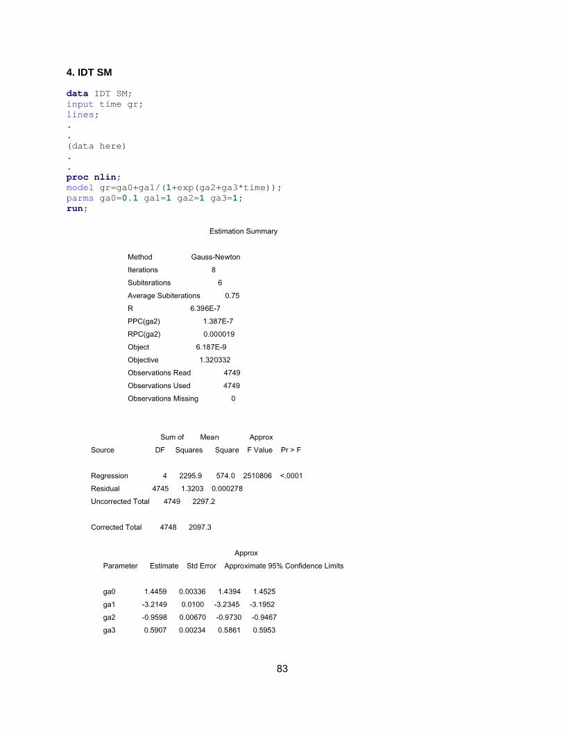
83

4. IDT SM data IDT SM; input time gr; lines; . . (data here) . . proc nlin; model gr=ga0+ga1/(1+exp(ga2+ga3*time)); parms ga0=0.1 ga1=1 ga2=1 ga3=1; run;

Estimation Summary Method Gauss-Newton Iterations 8 Subiterations 6 Average Subiterations 0.75 R 6.396E-7 PPC(ga2) 1.387E-7 RPC(ga2) 0.000019 Object 6.187E-9 Objective 1.320332 Observations Read 4749 Observations Used 4749 Observations Missing 0 Sum of Mean Approx Source DF Squares Square F Value Pr > F Regression 4 2295.9 574.0 2510806 <.0001 Residual 4745 1.3203 0.000278 Uncorrected Total 4749 2297.2 Corrected Total 4748 2097.3

Approx

Parameter Estimate Std Error Approximate 95% Confidence Limits ga0 1.4459 0.00336 1.4394 1.4525 ga1 -3.2149 0.0100 -3.2345 -3.1952 ga2 -0.9598 0.00670 -0.9730 -0.9467 ga3 0.5907 0.00234 0.5861 0.5953

84

VITA Myunggoo Jeong was born in Seoul, Korea, on October 15, 1972. He attended Sung Kyun

Kwan University with honor in 1991. One year after the completion of his undergraduate study,

he served in the Korean Air Force as part of required 30-month military service. After finishing

the military service, he resumed his undergraduate study and graduated with a Bachelor of

Science degree in Civil Engineering in 1998.

Upon graduation, he joined the Samsung Engineering Construction Company (SECC) as a civil

engineer. He worked at two construction sites where he built new and remodeled existing

highways. After four year of work, he decided to return to school and enrolled at Virginia

Polytechnic Institute and State University, Blacksburg, Virginia in August, 2003. He has served

as a graduate research assistant since 2004 under the direction of Dr. Flintsch and earned a

Master of Science Degree in Civil and Environmental Engineering in 2005. He intends to pursue

a Ph. D degree at Arizona State University from August 2005.