NORGES TEKNISK-NATURVITENSKAPELIGE

UNIVERSITET

Comparing positive predictive values

for small samples with applicationto gene ontology testing

by

Clara-Cecilie Gunther, Øyvind Bakke andMette Langaas

PREPRINT STATISTICS NO. 3/2009

DEPARTMENT OF MATHEMATICAL SCIENCES

NORWEGIAN UNIVERSITY OF SCIENCE ANDTECHNOLOGY

TRONDHEIM, NORWAY

This report has URL

http://www.math.ntnu.no/preprint/statistics/2009/S3-2009.pdf

Mette Langaas has homepage: http://www.math.ntnu.no/∼mettela

E-mail: Mette.Langaas@math.ntnu.no

Address: Department of Mathematical Sciences, Norwegian University of Science and

Technology, N-7491 Trondheim, Norway.

COMPARING POSITIVE PREDICTIVE VALUES FOR SMALL

SAMPLES WITH APPLICATION TO GENE ONTOLOGY TESTING

CLARA-CECILIE GÜNTHER, ØYVIND BAKKE AND METTE LANGAASDepartment of Mathematical Sciences.

The Norwegian University of Science and Technology,NO-7491 Trondheim, Norway.

MARCH 2009

SUMMARY

Motivated by the challenge of detecting Gene Ontology (GO) categories which are over-represented or depleted when comparing biological findings represented by two over-lapping listsof genes, we examine the performance of different statistical tests. One key feature with this typeof data is that the sample size at each GO category often is small and thus large sample asymptotictests are not suitable. We look at four different test statistics in combination with parametric boot-strapping, and compare the methods with their asymptotic alternatives. We find that the choice oftest statistic influence which GO categories are found to be significant, and all tests under studyperform increasingly conservative as the sample size decreases. We observe that this problem isstatistically the same as comparing the positive predictive values of two diagnostic tests.

1 INTRODUCTION

In some biological experiments the aim is, e.g. by using DNA microarrays, to discover genes that aredifferentially expressed between two or more conditions. The conditions may be defined by the pres-ence or absence of a disease or by different treatments like diets, drugs or amount of physical exercise.As an example we consider a situation where the relationship between inborn aerobic capacity andcardiac gene expression in rats was studied, Bye, Langaas, Høydahl, Kemi, Heinrich, Koch, Britton,Najjar, Ellingsen and Wisløff (2008). The rats were born with either high running capacity (HCR) orlow running capacity (LCR), and half of the rats were trained, while the others remained sedentary.Thus there were four groups of rats, LCR trained, LCR sedentary, HCR trained and HCR sedentary.Several comparisons were done, and the comparison of the gene expression for the sedentary HCR ratswith the gene expression for the sedentary LCR rats resulted in a list of 1540 differentially expressedgenes between these two groups.

However, since such lists contains only single genes, i.e. without information about potential con-nections to the other genes on the list, it can be challenging to interpret the biological meaning ofthe results. What may be more interesting for interpretation purposes is the biological pathways thatare active in the conditions under study. To do this, groups of genes instead of single genes areconsidered. In this paper we consider groups of genes selected from a predefined set using the GeneOntology (GO) vocabulary, The Gene Ontology Consortium (2000). GO is a vocabulary that classifies

1

genes into the three main categories: biological process, molecular function and cellular componentand their subcategories.

Given the list of differentially expressed genes from the experiment and the list of all genes present onthe microarray chip, called the master list, the biologist wants to know whether certain gene classesare over-represented or depleted in the list of differentially expressed genes compared to the masterlist. In the rat example, we are interested in knowing if the number of genes related to aerobic ca-pacity among those differentially expressed between the sedentary HCR rats and the sedentary LCRrats is higher than what we would expect by chance if we compare it to the master list. The list ofdifferentially expressed genes is contained in the master list, and the statistical hypothesis problem isto test whether two binomial proportions are equal. Common approaches are Pearson’s asymptoticχ2-test and Fisher’s exact test for large and small samples, respectively.

If there are more than two conditions in the experiment, several comparisons can be done which mayeach result in a list of differentially expressed genes between the conditions being compared. Thenwe would like to see whether some specific gene classes of interest are over-represented or depletedon one of the lists compared to one of the others. The two lists may either be mutually exclusive orpartly overlapping. If they are mutually exclusive the problem reduces to test whether two binomialproportions are equal as for the master list problem and the same approaches can be used. We willconsider only the situation of overlapping gene lists. In the rat example, we want to compare thelist of differentially expressed genes between trained HCR and LCR rats to the list of differentiallyexpressed genes between trained HCR rats and sedentary LCR rats.

Comparing two overlapping gene lists in terms of over-represented or depleted gene classes is sta-tistically the same situation as comparing the positive predictive values for two diagnostic tests andseveral hypothesis tests for this situation can be found in the literature, see Leisenring, Alonzo andPepe (2000), Wang, Davis and Soong (2006) and Moskowitz and Pepe (2006). Günther, Bakke,Lydersen and Langaas (2008) presented a likelihood ratio test and a restricted difference test andcompared them to the other existing tests. Simulation experiments showed that for smaller samplesizes these tests did not preserve their test size. When comparing gene lists, the actual sample size isthe number of genes associated with each of the three main GO-categories, not the number of geneson the microarray chip, nor the total number of genes on the lists. This number is usually quite smalland large sample tests are not a suitable approach. Instead small sample tests should be applied.

In this paper we evaluate small sample tests for comparing two overlapping gene lists, i.e. to testwhether the probabilities that a randomly chosen gene belongs to a specific gene class are equal forthe two lists. We first describe the assumed model and define the null and alternative hypothesesin Section 2, and then present the test statistics and how to calculate the p-values in Section 3. Asimulation study is conducted to assess the method and described in Section 4 and in Section 5 anexample in which data from the literature is given. A short discussion is given in Section 6 before weend with the conclusions in Section 7.

2 MODEL AND DATA

We assume that we have two lists of genes, list A and list B. For each gene we are interested incomparing the probability that it belongs to a certain gene class D given that it is on list A, withthe probability that it belongs to D given that it is on list B. Our null hypothesis is that these twoprobabilities are equal. By defining the three events

2

• D: The gene belongs to gene class D.

• A: The gene is present on gene list A.

• B: The gene is present on gene list B.

we can express the null hypothesis as

H0 : P (D | A) = P (D | B). (1)

Statistically, this is the same problem as testing equality of the positive predictive values of two diag-nostic tests for the same disease. Two diagnostic tests with binary outcomes, i.e. positive or negative,are applied to each subject in the study. The positive predictive value (PPV) is defined as the proba-bility that the subject has the disease of study given that the test is positive. If we let event D be thatthe subject has the disease, A the event that the outcome of test A is positive and B the event thatthe outcome of test B is positive, then the positive predictive value of test A is PPVA = P (D | A),and the positive predictive value of test B is PPVB = P (D | B). Our null hypothesis is that the twopositive predictive values are equal, i.e. H0 : P (D | A) = P (D | B) as in (1).

The Venn diagram in Figure 1 shows the six mutually exclusive events defined by A, B and D. Weonly look at the restricted sample space, i.e. A ∪ B, and thereby only the part of D that intersectsA ∪ B. Let A∗, B∗ and D∗ be the complementary events of A, B and D respectively. Günther et al.(2008) argue that when comparing positive predictive values it suffices to consider only the subjectswith at least one positive test result, which equals the setA∪B. In the GO setting the number of genesbelonging to the GO category D that are not present on any of the lists, i.e. the event (A∗ ∪B∗) ∩D,is unknown as is the number of genes not present on the lists that do not belong to the GO categoryD, therefore the part of D that intersects with A∗ ∪B∗ is not included.

To each of the six events in the Venn diagram there corresponds the probability qi that event i oc-curs, i = 1, ..., 6. The sum of these probabilities is one, i.e.

∑6i=1 qi = 1. Associated with each

event is also a random variable Ni, i = 1, . . . , 6, Ni being the number of times event i occurs. Weconsider one main category at a time, such that in total there are N =

∑6i=1Ni unique genes on

the two lists associated with either biological process, cellular component or molecular function. Thenumber N will typically change between the three main categories. Given N , the random variablesN1, N2, . . . , N6 are multinomially distributed with parameters N andq = (q1, q2, q3, q4, q5, q6). The joint probability function of N1, N2, . . . , N6 is

P

(6⋂

i=1

(Ni = ni)

)= N !

6∏i=1

qnii

ni!. (2)

The expected value of N = (N1, N2, N3, N4, N5, N6) is µ = E(N) = N · q and the covariancematrix is Σ = Cov(N) = N(Diag(q) − qTq), Johnson, Kotz and Balakrishan (1997). We do notassume that a random gene’s presence on list A is independent on its presence on list B and of whetherit belongs to GO category D. This is implicitly handled by the multinomial model, since each geneyields only one observation of one of the six mutually exclusive events. We do however assume thatthe genes are sampled independently of each other and we will comment this further in Section 6.

Throughout this work, we assume that only N is fixed and that N are realisations of multinomialsamples. Other sampling schemes are possible as well, for instance by fixing ND, NA and NB , the

3

number of genes belonging to gene class D, are present on list A and are present on list B respectively,and samplingN independently from three binomial distributions. In this report, we will not considerthese approaches.

The probabilities P (D|A) and P (D|B) can be expressed in terms of the parameters q since

P (D|A) =P (D ∩A)P (A)

=q4 + q5

q1 + q2 + q4 + q5

and

P (D|B) =P (D ∩B)P (B)

=q4 + q6

q1 + q3 + q4 + q6.

Thus, the null hypothesis can be written

H0 : δ =q4 + q5

q1 + q2 + q4 + q5− q4 + q6q1 + q3 + q4 + q6

= 0. (3)

N4

A

D

N2

N5

N1

N3

N6

B

FIGURE 1: Venn diagram for the events D, A and B showing which events the random variablesN1, . . . , N6 correspond to.

There are several possible alternative hypotheses. If we are interested in whether there is an en-richment or depletion of genes belonging to gene class D on list A compared to list B, we have thetwo-sided alternative

H1 : P (D|A) 6= P (D|B). (4)

If we are interested in testing only whether there is an enrichment of genes belonging to gene class Don list A compared to list B, we have the one-sided alternative

H1 : P (D|A) > P (D|B). (5)

When testing whether there is a depletion of genes belonging to gene class D on list A compared tolist B, the alternative hypothesis is

H1 : P (D|A) < P (D|B). (6)

In this work we will focus on the two sided alternative. We observe data n = (n1, n2, n3, n4, n5, n6)which are realizations of N = (N1, N2, N3, N4, N5, N6) and can be represented in a table as shownin Table 1.

4

Event D∗ D

A ∩B n1 n4

A ∩B∗ n2 n5

A∗ ∩B n3 n6

TABLE 1: The observed data classified by the events A, B and D.

3 METHOD

In this section we present the test statistics we considered to test whether the probability of a genebelonging to gene class D given that it is present on list A is equal to the probability of a genebelonging to gene class D given that it is present on list B. We also describe how to calculate thep-values.

3.1 TEST STATISTICS

To test the null hypothesis (3), we consider four test statistics: a likelihood ratio test statistic, a scoretest statistic and two difference test statistics. They have all been shown to be asymptotically χ2

1

distributed when the sample size is large, Casella and Berger (2002), Leisenring et al. (2000), Wanget al. (2006), but here we will use parametric bootstrapping to approximate their distribution under thenull hypothesis for small samples. We describe the test statistics briefly, more details can be found inGünther et al. (2008).

The likelihood ratio test statistic is

TLR = −2 · log(λ(N))

where λ(N) is the maximum likelihood of a multinomial sample under the null hypothesis dividedby the general maximum likelihood of the multinomial sample. LetQ denote the parameter space forq andQ0 the subspace ofQ in which q satisfy the constraint given by the null hypothesis (3). Then,

λ(n) =supQ0

L(q|n)

supQL(q|n).

Let qi, i = 1, . . . , 6, be the restricted maximum likelihood estimates, that is, the maximum likelihoodestimates underH0, and let qi, i = 1, . . . , 6 be the unrestricted general maximum likelihood estimatesfor the multinomial distribution, i.e. qi = ni/N . Inserting these estimates in the log-likelihoodfunction for the multinomial distribution leads to the test statistic

TLR = −2

(6∑

i=1

ni · (log qi − log qi)

). (7)

Note that qi, i = 1, . . . , 6, cannot be written in any comprehensible closed form, but can be foundusing an optimization routine or analytically by solving a Lagrangian system of equations. We do thelatter using Maple 12, for details see Günther et al. (2008).

5

The difference tests are based on the estimator g(N) for the difference δ in (3),

g(N) =N4 +N5

N1 +N2 +N4 +N5− N4 +N6

N1 +N3 +N4 +N6(8)

and the test statistic is derived by subtracting the expectation of g(N) and dividing by its approximatestandard deviation, which is found by taking the variance of the first order Taylor expansion of g(N).Let µ = E(N) and Σ = Cov(N) as defined in Section 2. This yields

Tg =(g(N)− g(µ))2

GT (µ)Σ G(µ)(9)

where G is a vector containing the first order partial derivatives of g(N) with respect to the compo-nents ofN and GT is the transpose of G. G(µ) is G with µ inserted forN .

Under the null hypothesis g(µ) = 0. G(µ) and Σ depend on the unknown parameters q which mustbe estimated when calculating the test statistic. We can either use the unrestricted maximum likelihoodestimates q for the multinomial distribution or the restricted maximum likelihood estimates q underH0. In the first case we refer to the test as the unrestricted difference test (uDT) and denote the teststatistic TuDT and in the second case we refer to the test as the restricted difference test (rDT) anddenote the test statistic TrDT.

Leisenring et al. (2000) presented a score test, which we denote the LAP test, for testing equivalenceof positive predictive values of two diagnostic tests, based on generalized estimating equations. Theydefine three indicator variables. First Dij indicates the disease status of subject i for diagnostic testj, i.e. Dij = 0 if the subject does not have the disease and Dij = 1 if it does have the disease.Zij indicates which test is used, it is 0 for test A and 1 for test B. Xij indicates the test result, it is0 if the test is negative and 1 if it is positive. Then the positive predictive value for test A can bewritten PPVA = P (Dij = 1 | Zij = 0, Xij = 1) and the positive predictive value for test B isPPVB = P (Dij = 1 | Zij = 1, Xij = 1). Leisenring et al. (2000) fit the generalized linear model

logit(P (Dij = 1 | Zij , Xij = 1)) = αP + βPZij ,

and test whether βP = 0 which is equivalent to testing whether PPVA = PPVB . We translate the testto the GO situation and in our notation the test statistic can be written as

TLAP =((N1 +N2 +N4 +N5)(N4 +N6)− (N1 +N3 +N4 +N6)(N4 +N5))2

f(N1, N2, N3, N4, N5, N6), (10)

6

where

f(N1, N2, N3, N4, N5, N6)

= N1(N2 −N3 +N5 −N6)2(

2N4 +N5 +N6

2N1 +N2 +N3 + 2N4 +N5 +N6

)2

+N2(N1 +N3 +N4 +N6)2(

2N4 +N5 +N6

2N1 +N2 +N3 + 2N4 +N5 +N6

)2

+N3(N1 +N2 +N4 +N5)2(

2N4 +N5 +N6

2N1 +N2 +N3 + 2N4 +N5 +N6

)2

+N4(N2 −N3 +N5 −N6)2(

1− 2N4 +N5 +N6

2N1 +N2 +N3 + 2N4 +N5 +N6

)2

+N5(N1 +N3 +N4 +N6)2(

1− 2N4 +N5 +N6

2N1 +N2 +N3 + 2N4 +N5 +N6

)2

+N6(N1 +N2 +N4 +N5)2(

1− 2N4 +N5 +N6

2N1 +N2 +N3 + 2N4 +N5 +N6

)2

.

The numerator can be found from by setting the difference in (8) equal to 0 and rearranging the terms.In the denominator, the number of genes that do not belong to GO category D, N1, N2 and N3, areeach multiplied by the proportion of genes that belong to the category D and in this proportion, thegenes that are present on both lists, N1 and N4, are given double weight. The number of genes thatbelong to GO category D, N4, N5 and N6, are each multiplied by the proportion of genes that do notbelong to the gene class D where the genes that are present on both lists are given double weight.

3.2 CALCULATION OF p-VALUES

We will use parametric bootstrapping to approximate the distribution of the test statistics under thenull hypothesis and find approximate p-values. The test statistic of interest, is either TLAP, TLR, TuDTor TrDT. To calculate the p-values we use the following algorithm:

1. For a given sample of size N , find the maximum likelihood estimates of the parameters underH0, q, and calculate the test statistic t for this sample, denoted ts.

2. Draw B samples from the multinomial distribution with parameters N and q.

3. Calculate the test statistic tk for each of these samples, 1 ≤ k ≤ B.

4. The p-value is given as∑B

k=1 I(tk ≥ ts), where I(tk ≥ ts) ={

1 if tk ≥ ts0 if tk < ts

, thus the p-

value is the proportion of simulated test statistics greater than or equal to the given test statistics.

4 ASSESSMENT OF METHOD

To assess the performance of the four tests in terms of test size, we perform a simulation study.The test size is the probability of making a type I error, i.e. for rejecting H0 when H0 is true. We

7

consider different sample sizes to evaluate the effect of N on the test size, and we also use severalparameter values of q in the multinomial distribution to explore different areas of the null hypothesis.All analysis are performed using the R language, R Development Core Team (2008), except findingthe maximum likelihood estimates under H0 which is done using Maple 12.

4.1 SIMULATION ALGORITHM

Given q and N , we draw M datasets from the multinomial distribution with parameters q and N . Foreach of these datasets we find the p-value using parametric bootstrapping as described in Section 3.2.

4.2 CASES UNDER STUDY

The data sets are generated from the parameters q in the multinomial distribution and we choose sixcases of parameters, given in Table 2 and depicted in Figure 2.

Case q1 q2 q3 q4 q5 q6

1 0.068 0.135 0.135 0.527 0.068 0.0682 0.043 0.130 0.130 0.348 0.174 0.1743 0.267 0.267 0.267 0.067 0.067 0.0674 0.300 0.267 0.267 0.033 0.067 0.0675 0.400 0.200 0.200 0.100 0.050 0.0506 0.450 0.200 0.200 0.050 0.050 0.050

TABLE 2: Specification of parameters in the simulation study.

The parameters in case 1 and 2 are motivated by the setting for diagnostic tests and chosen as describedin the multinomial simulation experiment of Günther et al. (2008). In case 3–6, we first set theprobabilities o1 = P (A ∩ B), o2 = P (A ∩ B∗) and o3 = P (A∗ ∩ B) and then p1 = P (D|A ∩ B),p2 = P (D|A ∩B∗) and p3 = P (D|A∗ ∩B). From these probabilities q are calculated as follows,

qi ={oi(1− pi) i = 1, 2, 3oipi i = 4, 5, 6.

In case 3 o1 = o2 = o3 = 1/3 and p1 = p2 = p3 = 1/5. In case 4 o1 = o2 = o3 = 1/3 andp1 = 1/10 while p2 = p3 = 2/10. The probabilities in case 5 are o1 = 1/2, o3 = o4 = 1/4 andp1 = p2 = p3 = 1/5. Finally, in case 6, o1 = 1/2, o2 = o3 = 1/4, p1 = 1/10 and p2 = p3 = 2/10.

The remaining parameter in the multinomial distribution, N , must also be chosen and since we areconsidering small sample sizes, we use N = 10, 15, 20 and 25. For each of the values of N all thecases given in Table 2 are run. In each of the six cases we draw M = 10000 samples and for each ofthese samples we draw B = 10000 bootstrap samples.

4.3 RESULTS

The test size is estimated as the proportion of p-values being less than or equal to the chosen nominallevel α. Let W be a random variable counting the number of p-values smaller than or equal to α.

8

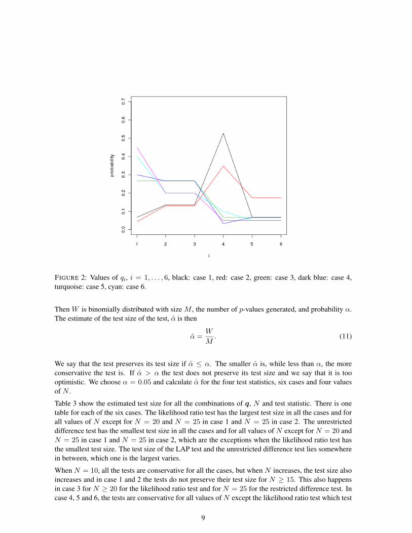
FIGURE 2: Values of qi, i = 1, . . . , 6, black: case 1, red: case 2, green: case 3, dark blue: case 4,turquoise: case 5, cyan: case 6.

Then W is binomially distributed with size M , the number of p-values generated, and probability α.The estimate of the test size of the test, α is then

α =W

M. (11)

We say that the test preserves its test size if α ≤ α. The smaller α is, while less than α, the moreconservative the test is. If α > α the test does not preserve its test size and we say that it is toooptimistic. We choose α = 0.05 and calculate α for the four test statistics, six cases and four valuesof N .

Table 3 show the estimated test size for all the combinations of q, N and test statistic. There is onetable for each of the six cases. The likelihood ratio test has the largest test size in all the cases and forall values of N except for N = 20 and N = 25 in case 1 and N = 25 in case 2. The unrestricteddifference test has the smallest test size in all the cases and for all values of N except for N = 20 andN = 25 in case 1 and N = 25 in case 2, which are the exceptions when the likelihood ratio test hasthe smallest test size. The test size of the LAP test and the unrestricted difference test lies somewherein between, which one is the largest varies.

When N = 10, all the tests are conservative for all the cases, but when N increases, the test size alsoincreases and in case 1 and 2 the tests do not preserve their test size for N ≥ 15. This also happensin case 3 for N ≥ 20 for the likelihood ratio test and for N = 25 for the restricted difference test. Incase 4, 5 and 6, the tests are conservative for all values of N except the likelihood ratio test which test

9

(a) Case 1

N LAP LRT rDT uDT10 0.042 0.046 0.039 0.03515 0.059 0.061 0.060 0.05720 0.063 0.061 0.062 0.06225 0.055 0.052 0.054 0.055

(b) Case 2

N LAP LRT rDT uDT10 0.038 0.043 0.040 0.01815 0.056 0.058 0.057 0.04720 0.056 0.057 0.057 0.05425 0.058 0.057 0.058 0.057

(c) Case 3

N LAP LRT rDT uDT10 0.014 0.028 0.026 0.00715 0.029 0.044 0.041 0.02420 0.041 0.055 0.051 0.03825 0.047 0.056 0.053 0.046

(d) Case 4

N LAP LRT rDT uDT10 0.012 0.023 0.021 0.00415 0.026 0.041 0.036 0.02020 0.035 0.047 0.044 0.02925 0.044 0.051 0.047 0.041

(e) Case 5

N LAP LRT rDT uDT10 0.010 0.022 0.020 0.00815 0.021 0.037 0.033 0.02020 0.032 0.042 0.039 0.03125 0.040 0.049 0.046 0.040

(f) Case 6

N LAP LRT rDT uDT10 0.007 0.013 0.012 0.00415 0.014 0.024 0.022 0.01120 0.029 0.037 0.034 0.02625 0.039 0.045 0.041 0.037

TABLE 3: Estimated test size, α, for α = 0.05. LAP denotes the LAP test, LRT the likelihood ratiotest and uDT and rDT denote the unrestricted and restricted difference test respectively.

size is 0.050 for N = 25 in case 4 and 6.

Figure 3 shows the estimated test size for the asymptotic methods plotted against the estimated testsize for the parametric bootstrap methods, there is one plot for each method for α = 0.05. If thepoints lie above the diagonal line, the test size of the asymptotic test is higher than the test size ofthe parametric bootstrap test, and lower if the points are below the line. If the points lie above thehorizontal line the test size for the asymptotic test is greater than α = 0.05 and smaller if they liebelow the line. Similarly, for the points that lie to the right of the vertical line, the test size for theparametric bootstrap test is higher than 0.05 and it is lower than 0.05 if they lie to the left of this line.

We note in particular that for all the cases and for all values of N , the test size for the parametricbootstrap restricted difference test is greater than the test size for the large sample restricted differencetest. For the likelihood ratio test, the opposite is true, the test size of the asymptotic likelihood ratiotest is greater than the test size of the parametric bootstrap likelihood ratio test. This indicates thatthe parametric bootstrap test is an improvement compared to the asymptotic likelihood ratio test forsmall samples. However, the asymptotic likelihood ratio test does not preserve its test size in 15 ofthe 24 combinations of N and q and in six of those the parametric bootstrap test is still too optimistic.To use the parametric bootstrap restricted difference test does not yield an improvement compared tousing the asymptotic restricted difference test.

Figure 4 shows the observed level, i.e. the test size, of the tests plotted against the nominal level forN = 10, 15, 20, 25 in case 3 for a chosen nominal level in the range from 0 to 0.10. We see that thetest size increases when N increases and also that the tests yield more similar results for the highervalues of N . The unrestricted difference test and the LAP test preserve the test size in all the caseswhile the likelihood ratio test is too optimistic when N = 20 or 25.

10

(a) (b)

(c) (d)

FIGURE 3: Estimated test size for the asymptotic versus the small sample tests, for different values ofN : Red=10, green=15, dark blue=20, cyan=25.

11

(a) (b)

(c) (d)

FIGURE 4: Observed level versus nominal level for (a)N = 10, (b)N = 15, (c)N = 20, (d)N = 25,green = LRT, red = LAP, dark blue = rDT, grey = uDT.

12

5 EXAMPLE FROM GENE ONTOLOGY

As an example of how the tests perform on a data set from literature, we use part of the data presentedby Bye et al. (2008). To estimate the effect of running capacity of the trained rats, we compare thegene expression for the HCR trained rats with the LCR trained rats. This gives us a list of differentiallyexpressed genes between these two groups, we call this list A. It may be of interest to estimate the jointeffect of training and inbread running capacity by comparing the trained HCR rats versus the sedentaryLCR rats. This gives us another list of differentially expressed genes which we call list B. To determinewhich genes are differentially expressed a cut-off must be chosen. For each gene, a p-value and anadjusted p-value are calculated. The adjusted p-values are adjusted using the Benjamini-Hochbergstep-up procedure to control the false discovery rate (FDR), Benjamini and Hochberg (1995). Thecut-off is chosen such that all the genes that have a p-value smaller than or equal to this value are saidto be differentially expressed. We will use two different cut-offs and first we choose an FDR cut-off of0.025 for both lists, which yields 12 genes on list A and 24 genes on list B. These lists are submittedto eGOn, Beisvåg, Jünge, Bergum, Jølsum, Lydersen, Günther, Ramampiaro, Langaas, Sandvik andLægreid (2006), a web-based tool that automatically translates the lists to GO categories. We areinterested in genes annotated to the main category molecular function. There are three genes from thefirst list and nine genes from the second list annotated to this category. Of these genes two are on bothlist A and B and therefore there are N = 10 unique genes on the two lists associated with molecularfunction.

The GO tree has several levels corresponding to the hierarchy of the GO categories. One gene canbelong to more than one GO category, and given that it belongs to a subcategory it will also belongto the parent categories of this subcategory on the upper levels. After submitting the lists, one has tochoose which main category to consider, i.e. either molecular function, biological process or cellularcomponent. Level 1 is the main category itself with no subcategories, e.g. molecular function. Thehigher level number is chosen, the more subcategories are included, and they are all subcategories ofthe chosen main category. We choose to display the GO tree at level 3 for the main category molecularfunction and Table 4 shows the 11 GO categories that are represented on the lists, i.e. the categorieswhich the genes on the lists belong to. A hypothesis test is performed for each category, testingwhether it is over-represented or depleted on one of the lists compared to the other list.

If we use an FDR cut-off of 0.05 on differential expression instead we get two lists of 30 and 63 genes,42 of these genes can be classified under the main category molecular function. Within this category,seven genes are present on both lists, seven genes are present only on list A and 21 genes are presentonly on list B, yielding N = 35 unique genes. Table 5 shows the GO categories for these genes alongwith their p-values.

Table 4 and 5 both include a column with the p-value calculated by eGOn. These p-values are cal-culated using the asymptotic LAP test. We calculate the p-values for the three other tests, i.e. thelikelihood ratio test and the restricted and unrestricted difference test using parametric bootstrappingand compare them to the asymptotic p-values for all four tests. When performing the bootstrappingwe draw B = 10000 bootstrap samples for each GO category.

Table 6 shows the results for the FDR cut-off of 0.025. The GO category ion binding (GO:0043167)is significant when using either the parametric bootstrap or asymptotic likelihood ratio or restricteddifference test. It is also significant when using the asymptotic unrestricted difference test, whileit is not significant when using the parametric bootstrap or asymptotic LAP test or the asymptoticunrestricted difference test. None of the other GO categories are significant for any of the tests.

13

GO identifier Name p-value n4 n5 n6

GO:0005488 binding 0.157 2 1 5GO:0030246 carbohydrate binding 0.273 1 0 0GO:0043167 ion binding 0.077 1 1 0GO:0008289 lipid binding 0.279 0 1 0GO:0003676 nucleic acid binding 0.317 0 0 1GO:0005515 protein binding 0.705 2 0 5GO:0046906 tetrapyrrole binding 0.279 0 1 0GO:0003824 catalytic activity 0.245 1 1 2GO:0016787 hydrolase activity 0.273 1 0 0GO:0016874 ligase activity 0.317 0 0 1GO:0016491 oxidoreductase activity 0.46 0 1 1

TABLE 4: GO categories within molecular function with their corresponding p-values and number ofgenes on the lists.

When considering only the parametric bootstrap tests, in general the likelihood ratio test and restricteddifference test give similar p-values which in some cases are smaller than the p-values for the LAPtest and the unrestricted difference test. One example is the GO category lipid binding (GO:0008289)where the p-values are 0.160, 0.065, 0.065 and 0.220 for the LAP, likelihood ratio, restricted differenceand unrestricted difference tests respectively. Even though lipid binding is not significant for any ofthese tests, it is not far from being significant for the LRT and rDT tests which is not the case forthe LAP and unrestricted difference tests. Together with the example ion binding, this indicates thata GO category may be declared significant more often for the likelihood ratio test and restricteddifference tests than with the LAP and unrestricted difference tests. This coincide with the findings inthe simulation experiments where the estimated test size in several cases were higher for the likelihoodratio and restricted difference tests than for the LAP and uDT tests.

Table 7 shows the results for the FDR cut-off of 0.05. The GO category catalytic activity (GO:0003824)is significant with a p-value <0.05 for all the tests, both the parametric bootstrap and asymptotic tests.The GO category hydrolase activity (GO:0016787) is significant when using the parametric bootstrapLRT or rDT tests and when using the asymptotic LRT, rDT and uDT tests. We see the same for the GOcategory substrate-specific transporter activity (GO:0022892), except that it is not significant using theasymptotic uDT test. We note that the category ion binding which is significant when we use an FDRcut-off of 0.025 is not significant now. In general, for the parametric bootstrap tests, the LRT and rDTtests yield similar p-values that are often smaller than the p-values for the LAP and uDT tests. Thedifference between the p-values can be quite large and for the GO term lipid binding (GO:0008289)the p-values are 0.179, 0.0345, 0.036 and 0.188 for the LAP, likelihood ratio, restricted differenceand urestricted difference tests respectively. This example shows that the choice of test statistic iscritical when finding GO categories that are significantly over-represented or depleted in one gene listcompared to the other list. The differences between the parametric bootstrap and asymptotic tests donot follow a clear pattern, for some GO categories the parametric bootstrap p-values are smaller, forother GO categories they are greater.

The GO category chromatin binding (GO:0003682) was found to be significantly over-represented onthe list of differentially expressed genes between HCR and LCR sedentary rats, using an FDR cut-off

14

GO identifier Name p-value n4 n5 n6

GO:0005488 binding 0.651 5 7 18GO:0030246 carbohydrate binding 0.325 1 0 0GO:0003682 chromatin binding 0.313 0 0 1GO:0043167 ion binding 0.13 3 1 1GO:0008289 lipid binding 0.161 1 1 0GO:0003676 nucleic acid binding 0.485 1 1 5GO:0000166 nucleotide binding 0.518 1 2 3GO:0005515 protein binding 0.544 4 6 14GO:0046906 tetrapyrrole bindin 0.308 0 1 0GO:0003824 catalytic activity 0.016 5 5 6GO:0016787 hydrolase activity 0.059 1 4 2GO:0016874 ligase activity 0.56 1 0 2GO:0016829 lyase activity 0.325 1 0 0GO:0016491 oxidoreductase activity 0.226 2 1 1GO:0016740 transferase activity 1 1 0 1GO:0030234 enzyme regulator activity 0.325 1 0 0GO:0030695 GTPase regulator activity 0.325 1 0 0GO:0060089 molecular transducer activity 0.325 1 0 0GO:0004871 signal transducer activity 0.325 1 0 0GO:0005198 structural molecule activity 1 1 0 1GO:0005201 extracellular matrix structural constituent 0.325 1 0 0GO:0008307 structural constituent of muscle 0.313 0 0 1GO:0030528 transcription regulator activity 0.388 1 1 1GO:0003702 RNA polymerase II transcription factor activity 0.325 1 0 0GO:0003700 transcription factor activity 0.388 1 1 1GO:0016564 transcription repressor activity 0.325 1 0 0GO:0005215 transporter activity 0.168 1 2 1GO:0022892 substrate-specific transporter activity 0.073 1 2 0GO:0022857 transmembrane transporter activity 0.168 1 2 1

TABLE 5: GO categories within molecular function with their corresponding p-values and number ofgenes on the lists.

15

Parametric bootstrap AsymptoticGO identifier LAP LRT rDT uDT LAP LRT rDT uDTGO:0005488 0.198 0.315 0.344 0.204 0.157 0.249 0.354 0.109GO:0030246 0.162 0.072 0.067 0.179 0.273 0.127 0.132 0.257GO:0043167 0.054 0.004 0.007 0.072 0.077 0.010 0.012 0.021GO:0008289 0.160 0.065 0.065 0.220 0.279 0.074 0.065 0.221GO:0003676 0.383 0.371 0.401 0.446 0.317 0.433 0.540 0.289GO:0005515 0.845 0.803 0.817 0.805 0.705 0.687 0.683 0.699GO:0046906 0.146 0.062 0.062 0.206 0.279 0.074 0.065 0.221GO:0003824 0.338 0.263 0.219 0.448 0.245 0.207 0.213 0.194GO:0016787 0.164 0.073 0.065 0.181 0.273 0.127 0.132 0.257GO:0016874 0.390 0.375 0.402 0.454 0.317 0.433 0.540 0.289GO:0016491 0.678 0.454 0.299 0.714 0.460 0.376 0.353 0.431

TABLE 6: Parametric bootstrap and asymptotic p-values for the subcategories of molecular function.

of 0.05, compared to the list of all genes by Bye et al. (2008). Another GO category, nucleic acidbinding (GO:0003676) was significantly over-represented on the list of genes that were significantlymore expressed for HCR rats than for LCR rats compared to the list of genes that were significantlymore expressed for LCR rats than for HCR rats, Bye et al. (2008). None of these GO-categoriesare over-represented in our two lists, but since we are not comparing the gene expression betweensedentary HCR and LCR rats it is not surprising.

Instead of comparing the comparison of gene expression for the HCR trained rats and the LCR trainedrats to the comparison of trained HCR rats and sedentary LCR rats, we could have compared the geneexpression of trained LCR rats with the gene expression of the sedentary LCR rats directly. This isdone in Bye et al. (2008). The list of differentially expressed genes is then submitted to eGOn andcompared to the master list. However, with an FDR cut-off of 0.05 the comparison results in only onegene on the list and this gene is not annotated to any GO category.

With the first FDR cut-off of 0.025, we compared the two lists at 11 GO categories and with the secondFDR cut-off at 0.05 we compared the lists at 29 GO categories. The problem thus involves multipletesting, and the p-values should be adjusted accordingly. This has not been done when comparing themethods and the p-values in Table 6 and 7 are therefore unadjusted.

6 DISCUSSION

To obtain list of differentially expressed genes, a cut-off on the differential expression must be set.The lists can then be submitted to a GO tool, e.g. eGOn, to discover GO categories that are over-represented or depleted. This approach has been criticised, see Goeman and Bühlman (2007) for anoverview. Firstly, it is not clear where the cut-off should be set and secondly, one may argue that allthe data should be used. Other proposed methods address this problem by either using all the p-valuesfrom the experiment or use raw expression data instead of p-values, see Goeman and Bühlman (2007).

The statistical tests in this report all treat the genes as the sampling units and are based on the as-sumption that the genes on the lists act independently under the null hypothesis. Statistically, it would

16

Parametric bootstrap AsymptoticGO identifier LAP LRT rDT uDT LAP LRT rDT uDTGO:0005488 0.670 0.672 0.676 0.667 0.651 0.652 0.657 0.649GO:0030246 0.369 0.180 0.171 0.371 0.325 0.240 0.308 0.326GO:0003682 0.382 0.393 0.407 0.403 0.313 0.363 0.472 0.309GO:0043167 0.124 0.113 0.075 0.128 0.130 0.095 0.091 0.127GO:0008289 0.179 0.034 0.036 0.188 0.161 0.053 0.075 0.152GO:0003676 0.511 0.528 0.535 0.512 0.485 0.500 0.510 0.483GO:0000166 0.544 0.528 0.516 0.544 0.518 0.498 0.491 0.515GO:0005515 0.561 0.564 0.568 0.559 0.544 0.547 0.552 0.541GO:0046906 0.182 0.091 0.082 0.190 0.308 0.132 0.151 0.299GO:0003824 0.017 0.017 0.016 0.020 0.016 0.015 0.016 0.011GO:0016787 0.093 0.043 0.022 0.094 0.059 0.029 0.027 0.046GO:0016874 0.606 0.612 0.609 0.606 0.56 0.559 0.568 0.557GO:0016829 0.378 0.175 0.167 0.38 0.325 0.240 0.308 0.326GO:0016491 0.262 0.227 0.166 0.262 0.226 0.180 0.175 0.222GO:0016740 1.000 0.871 1.000 1.000 1.000 1.000 1.000 1.000GO:0030234 0.372 0.182 0.172 0.375 0.325 0.240 0.308 0.326GO:0030695 0.368 0.18 0.171 0.371 0.325 0.240 0.308 0.326GO:0060089 0.374 0.178 0.168 0.378 0.325 0.240 0.308 0.326GO:0004871 0.371 0.176 0.166 0.373 0.325 0.240 0.308 0.326GO:0005198 1.000 0.876 1.000 1.000 1.000 1.000 1.000 1.000GO:0005201 0.366 0.173 0.164 0.37 0.325 0.240 0.308 0.326GO:0008307 0.377 0.382 0.393 0.394 0.313 0.363 0.472 0.309GO:0030528 0.501 0.422 0.349 0.501 0.388 0.340 0.33 0.384GO:0003702 0.364 0.180 0.168 0.366 0.325 0.240 0.308 0.326GO:0003700 0.494 0.418 0.346 0.493 0.388 0.340 0.33 0.384GO:0016564 0.373 0.180 0.169 0.376 0.325 0.240 0.308 0.326GO:0005215 0.236 0.134 0.079 0.237 0.168 0.107 0.101 0.157GO:0022892 0.064 0.008 0.009 0.055 0.073 0.012 0.019 0.062GO:0022857 0.234 0.132 0.081 0.234 0.168 0.107 0.101 0.157

TABLE 7: Parametric bootstrap and asymptotic p-values for the subcategories of molecular function.

17

be more intuitive to use the subjects as the sampling units, as discussed by Goeman and Bühlman(2007). Indeed, when testing for equality of the positive predictive values of two diagnostic tests,the observational unit is the individual and the assumption of independence of test results betweenindividuals is in most cases not seen to be problematic. But in the gene class setting the assumptiondoes not hold, because genes act together in pathways and genes that are functionally related can bestrongly correlated. If the gene expression measurements are correlated, the p-values tend to be pos-itively correlated, see Goeman and Bühlman (2007). A possible extension of the methods developedin this report could be to look at different dependence structures between the observational units.

We have considered test statistics designed for comparing positive predictive values for diagnostictests which translates to comparing association with GO categories for overlapping gene lists. Otherpossible approaches to handle overlapping gene lists include deleting the genes that are on both listsfrom each list or simply ignore the fact that there are genes that are on both lists and treat them asmutually exclusive lists. The deletion approach is implemented in the GO tool FatiGO, Al Shahrour,Diaz Uriarte and Dopazo (2004), in which Fisher’s exact test is implemented. In the ignore approachFisher’s exact test or Pearson χ2 test can be used. The asymptotic LAP test is implemented in eGOnwhich then handles the problem of overlapping gene lists more correctly than other GO-tools by notdeleting the genes that are on both lists or ignore that the genes are overlapping.

In the simulation experiments in Section 4 and the example using data from the literature in Section5, we see that the likelihood ratio and restricted difference tests yields similar results which differfrom the LAP and unrestricted difference tests. The likelihood ratio and restricted difference test bothuse the maximum likelihood estimates for the parameters under the null hypothesis in addition to thegeneral maximum likelihood estimates. The LAP and unrestricted difference also yield similar testresults and these test statistics are functions of the observed data n and thereby the general maximumlikelihood estimates only, and are thus not influenced by the maximum likelihood estimates under thenull.

When considering small sample sizes, one or more of the cells in Table 1 have often zero countswhich leads to non-computable test statistics for the LAP and difference tests. In these cases, we setthe test statistics to 0 if the numerator is 0, implying that the null hypothesis will never be rejected forsuch tables. If only the denominator is 0, the test statistic is disregarded. For N = 10 there are 18out of 3003 possible tables for which this will happen, while if N = 15 it will happen for 28 out of15504 tables, for N = 20 for 38 of 53130 tables and for N = 25 for 48 of 142506 outcomes. For thelikelihood ratio test statistic zero counts does not represent a problem, it can always be calculated. Ifany of the counts are 0, the summation term in (7) is also 0.

While the methodology in the present paper does not rely on asymptotic results, it is still approxima-tive in the sense that it relies on simulations. Another shortcoming is that the test size is not preservedin general. Both these issues will be addressed in a forthcoming paper, Günther, Bakke, Rue andLangaas (2009), where enumeration rather than simulation will be applied to the testing method ofthe present paper and where it will be modified to yield p-values that preserve the test size. The testsize and power will be calculated exactly.

7 CONCLUSIONS

In this report we look at the problem of testing the null hypothesis given in (3) when the samplesize is small. The large sample tests using asymptotic distributions do not preserve their test size in

18

this case and therefore small sample tests are needed. We suggest using parametric bootstrapping toapproximate the distribution and to calculate the p-values. The likelihood ratio test and the restricteddifference test are both functions of the maximum likelihood estimates q under the null hypothesiswhich may be difficult to find because of local optima. Especially zero counts causes problems, butour method that analytically solves the system of equations handles these problems well.

The simulation experiments show, at least based on the present six cases, that the small sample like-lihood ratio test yields a smaller test size than the large sample likelihood ratio test, while for therestricted difference test the large sample test yields the smallest test size and is still conservative,thus for this test there was no improvement.

For testing whether there is a difference in enrichment or depletion of genes belonging to a certainGO category between two list of genes from a microarray experiment, there are several test statisticsto choose from, and depending on the sample size, one can use either parametric bootstrapping orthe asymptotic χ2

1 distribution to calculate p-values. The choice of test statistic can influence whichGO categories that are found to be significant and because the small sample parametric bootstraplikelihood ratio and restricted difference tests are more optimistic than the small sample parametricbootstrap LAP and unrestricted difference tests, the first two will yield more significant GO categoriesthan the other two. The smaller the sample size is, the more conservative all the tests are which meansthey will not reject the null hypothesis even when it is not true., i.e. the tests will not discover geneclasses that are over-represented or depleted on one list compared to the other list. Therefore, para-metric bootstrapping does not seem to be an optimal solution and a better approach would probablybe to use an exact small sample test that preserves its test size without being conservative, which willbe investigated further.

REFERENCES

Al Shahrour, F., Diaz Uriarte, R. and Dopazo, J. (2004). FatiGO: a web tool for finding significantassociations of Gene Ontology terms with groups of genes, Bioinformatics 20(4): 578–580.

Beisvåg, V., Jünge, F. K., Bergum, H., Jølsum, L., Lydersen, S., Günther, C.-C., Ramampiaro, H.,Langaas, M., Sandvik, A. K. and Lægreid, A. (2006). GeneTools - application for functionalannotation and statistical hypothesis testing, BMC Bioinformatics 7(470).

Benjamini, Y. and Hochberg, Y. (1995). Controlling the false discovery rate: a practical and powerfulapproach to multiple testing, Journal of the Royal Statistical Society 57: 289–300.

Bye, A., Langaas, M., Høydahl, M. A., Kemi, O. J., Heinrich, G., Koch, L. G., Britton, S. L., Najjar,S. M., Ellingsen, Ø. and Wisløff, U. (2008). Aerobic capacity-dependent differences in cardiacgene expression., Physiol Genomics 33: 100–109.

Casella, G. and Berger, R. L. (2002). Statistical inference, second edn, Duxbury, chapter 8.

Goeman, J. J. and Bühlman, P. (2007). Analyzing gene expression data in terms of gene sets: method-ological issues., Bioinformatics 23(8): 980–987.

Günther, C.-C., Bakke, Ø., Lydersen, S. and Langaas, M. (2008). Comparison of predictive valuesfrom two diagnostic tests in large samples. Preprint Statistics No. 9, Department of MathematicalSciences, Norwegian University of Science and Technology.

19

Günther, C.-C., Bakke, Ø., Rue, H. and Langaas, M. (2009). Statistical hypothesis testing for cate-gorical data using enumeration in the presence of nuisance parameters. Preprint Statistics No. 4,Department of Mathematical Sciences, Norwegian University of Science and Technology.

Johnson, N. L., Kotz, S. and Balakrishan, N. (1997). Discrete multivariate distributions, Wiley seriesin probability and statistics, chapter 35.

Leisenring, W., Alonzo, T. and Pepe, M. S. (2000). Comparisons of predictive values of binarymedical diagnostic tests for paired designs, Biometrics 56: 345–351.

Moskowitz, C. S. and Pepe, M. S. (2006). Comparing the predictive values of diagnostic tests: samplesize and analysis for paired study designs, Clinical Trials 3: 272–279.

R Development Core Team (2008). R: A language and environment for statistical computing, RFoundation for Statistical Computing, Vienna, Austria.http://www.r-project.org

The Gene Ontology Consortium (2000). Gene Ontology: tool for the unification of biology, NatureGenetics 25: 25–29.

Wang, W., Davis, C. S. and Soong, S.-J. (2006). Comparison of predictive values of two diagnos-tic tests from the same sample of subjects using weighted least squares, Statistics in Medicine25: 2215–2229.

20