Company Stock Reacts to the 2016 Election Shock: Trump ... · Company Stock Reactions to the 2016...

Mossavar-Rahmani Center for Business & Government

Weil Hall | Harvard Kennedy School | www.hks.harvard.edu/mrcbg

Company Stock Reacts to the 2016 Election Shock:

Trump, Taxes and Trade

Alexander F. Wagner University of Zurich

Richard J. Zeckhauser Harvard Kennedy School

Alexandre Ziegler University of Zurich

2017

M-RCBG Faculty Working Paper Series | 2017-01

Mossavar-Rahmani Center for Business & Government Weil Hall | Harvard Kennedy School | www.mrcbg.org

The views expressed in the M-RCBG Associate Working Paper Series are those of the author(s) and do

not necessarily reflect those of the Mossavar-Rahmani Center for Business & Government or of

Harvard University. The papers in this series have not undergone formal review and approval; they are

presented to elicit feedback and to encourage debate on important public policy challenges. Copyright

belongs to the author(s). Papers may be downloaded for personal use only.

Company Stock Reactions to the 2016 Election Shock:

Trump, Taxes and Trade*

February 10, 2017

Alexander F. Wagner1

Richard J. Zeckhauser2

Alexandre Ziegler3

Abstract

Donald Trump’s election was a significant surprise. The reaction of company stock prices to the

election reflects shifts in investor expectations about economic growth, taxes, and trade policy.

High-beta stocks outperformed, presumably due to strengthened growth expectations.

Expectations of significant corporate tax cuts boosted high-tax firms, but hurt firms with

significant net operating loss carryforward balances. Investors currently perceive the climate to

be more favorable for domestically-oriented companies than those with substantial foreign

involvement. Markets incorporated expectations on growth and tax policy into stock prices

relatively quickly; they took more time to digest the consequences of shifts in trade policy.

JEL Classification: G12, G14, H25, O24

Keywords: Stock returns, event study, corporate taxes, trade policy, corporate interest payments,

post-news drift, election surprise

* We particularly thank Larry Summers for helpful comments. Wagner thanks the Swiss Finance Institute and the

University of Zurich Research Priority Program Financial Market Regulation for financial support. Wagner is

chairman of SWIPRA, and an independent counsel for PricewaterhouseCoopers. 1 Swiss Finance Institute -- University of Zurich, CEPR, and ECGI. Address: University of Zurich, Department of

Banking and Finance, Plattenstrasse 14, CH-8032 Zurich, Switzerland. Email: [email protected]. 2 Harvard University and NBER. Address: Harvard Kennedy School, 79 JFK Street, Cambridge, MA 02139, USA.

Email: [email protected]. 3 University of Zurich. Address: University of Zurich, Department of Banking and Finance, Plattenstrasse 14, CH-

8032 Zurich, Switzerland. Email: [email protected].

mailto:[email protected]



1

1 Introduction

The election of Donald J. Trump as the 45th President of the United States of America on

November 8, 2016 surprised most observers. The election’s unexpected outcome1 combined with

the wide policy differences between the two candidates led to substantial reactions on financial

markets. Large price moves were recorded across asset classes, including stocks, bonds, and

exchange rates. While analyst commentary on the implications of this historic election for

individual firms or industries abounds, to our knowledge, no academic study has investigated

which industries and firms will benefit or suffer under the new administration. Assessing the

winners and losers from the election is interesting, because there were sizable differences in the

policies favored by the two candidates in at least four economically important areas: government

spending (and the size of the deficit), taxation, trade policy, and regulation.

This paper uses the reactions of individual stock prices during the days and weeks following

the election to identify the relative winners and losers from the Trump administration’s expected

policies. In an era where politics is extremely polarized and forward-looking assessments of

economic prospects are often tilted and exaggerated, it is instructive to investigate investors’

assessment of the prospects for different firms and industries.

While there is a large literature on the effect of elections on financial markets, the 2016

Presidential election is particularly interesting because it is rare, in developed economies, to have

an instance of such a surprising outcome when the two candidates favored such disparate

policies.2 What is more, with the notable exception of the Mexican Peso, changes in the prices of

many assets following the election were the opposite of those that had been forecast if Trump

were to win. This occurred even though the forecasts had a strong empirical foundation. For

instance, in a study of asset price moves during the first Presidential debate on September 26,

2016, Wolfers and Zitzewitz (2016) had found a strong positive relationship between the odds of

Clinton winning on Betfair and the returns on all major US equity index futures. While stock

index futures fell sharply on election night as the outcome of the election became known, stock

1 On the morning of Election Day, Trump’s chances were 17% on Betfair and 28% on 538Silver. 2 For example, Niederhoffer, Gibbs, and Bullock (1970) consider Dow Jones Industrial Average responses to

elections and nominating conventions. Moreover, a substantial literature studies the stock market development

during Democratic and Republican administrations over the longer run. For example, Santa-Clara and Valkanov

(2003) document a “presidential premium” (especially for large-cap stocks) during Democratic presidencies.

2

markets finished up on the day following the election and rallied strongly during the rest of the

year and beyond.

It is impossible to determine whether the market’s rally will continue beyond the time of this

writing, nor whether developments to date have been due to overall beliefs about the economy

and firm fundamentals, to the view that a Trump administration will be good for business (e.g.,

much lower corporate taxes and reduced regulation), and/or just some combination of excess

animal spirits and group exuberance. As such, the “Trump Rally” isn’t that unusual: the overall

market tends to rise after elections historically. What is surprising about the post-election rally is

its magnitude, and its sharp difference from the significant decline that most forecasters had

predicted if Trump won the election.

It is also impossible to diagnose the reasons for a particular overall movement in the stock

market, as there is just one observation. Recognizing this, this paper investigates the differential

performance of a large number of stocks to determine which factors produced relative winners

and relative losers among companies as the stock market moved sharply upward after the

election. These results shed some light on the effect of expectations about policy, particularly

taxation, trade policy, and regulation – on individual firms. At the industry level, the stock

market reactions from the day after the election through the end of the year broadly follow

expected benefits and costs relative to the alternative outcome, the election of Hillary Clinton.

Heavy industry (which Trump has promised to resurrect) and financial firms, which he has said

he would deregulate, performed well. By contrast, healthcare, medical equipment, and

pharmaceuticals lost dramatically (presumably due to the expectation that Obamacare would be

dismantled or at least significantly altered), as did textile and apparel firms, reflecting their

significant dependence on imports, which Trump has vowed to strongly discourage. Business

supplies and shipping containers also lost, probably reflecting his tough stance on trade. It is

noteworthy that even after controlling for the rally in the broad market, several low-beta

industries (beer, tobacco, food products, utilities) were losers, while cyclical industries tended to

be winners. Presumably, expectations of higher growth induced investors to rotate from low-risk

to high-beta industries.

All assessments of industries or companies below address relative not absolute assessments,

since the stock market was up so dramatically, implying that many relative losers actually gained

in price, but not nearly so much as relative winners. Turning to the different policy areas, we find

3

evidence that both growth prospects and expectations of a major corporate tax cut were viewed

positively by the stock market. Specifically, firms with high beta, high tax rates, and high

deferred tax liabilities benefited, while those with tax loss carryforward balances lost. By

contrast, the stock market’s reactions imply negative expectations about the effects of the

incoming administration’s anticipated policies for internationally-oriented firms. Interestingly,

markets did not process information on these various aspects at the same speed. While the

positive impacts of corporate tax cuts and higher growth were apparent in the cross-section of

stock returns on the first day after the election, the negative impact of expected policy changes

on internationally-oriented firms mostly became felt later on. Investors also downgraded

companies with high interest expenses. This result does not necessarily have to do with an

expectation regarding interest deductibility being abolished (as is the case under some

Trump/Republican plans), as deductions also lose value when taxes are cut. Investors thus far

think that expensing capital investments is either unlikely to be implemented, or not

consequential.

2 Asset price responses to news

If the market responds optimally to the election outcome, the change in the market price of any

asset will reflect both the difference in its expected discounted payoff between the two possible

outcomes and the ex ante probability of the outcome. The advantage of considering asset price

changes is that they capture current expectations; the researcher need not trace all the future

changes to cash flows and discount rates separately (Schwert 1981). Formally, let PC and PT

denote the asset’s expected price conditional on Clinton and Trump winning, respectively,

implying that C and T = 1 – C are the probabilities of the two outcomes. Ignoring discounting

over the short period at hand, and assuming that risk aversion is a minor factor,3 the asset’s price

before the election is given by

TTCC PPP .

The price change for the asset given that Trump won is given by

3 Risk aversion on overall market movements would, of course, be reflected in beta. Stocks expected to perform

better in an unfavorable overall outcome would be priced higher and vice versa.

4

)1)(( TCTT PPPPP .

In words, the price change once the election results become known is the difference in prices

between the two outcomes, times the size of the election surprise, which is one minus the ex ante

probability of Trump winning. Intuitively, if Trump’s election had been certain ex ante, there

would have not have been a price reaction on the day after the election. Scaling this expression

by the initial price, the return on the asset once the election results become known is given by

P

PP

P

PPR TCTT )1)((

.

Note that while the election surprise is the same for all assets, individual assets will respond

to the election outcome differently, depending on the sign and magnitude of the spread between

PC and PT. For assets that would have benefitted from a Clinton outcome relative to Trump, PC >

PT, with the inequality reversed for assets that would be helped by a Trump outcome. To presage

some of our findings, stocks had very different reactions to the outcome. By considering the

cross-section of stock returns, we can thus infer whether the incoming administration’s expected

policies are viewed as favorable or not for a particular firm or industry, and the extent and speed

with which markets incorporated differences between the candidates in the different policy

dimensions into prices.

Two factors make the 2016 Presidential election an ideal setting for such an analysis. First,

there was a significant gap between the pre-election probabilities and the election outcome.

Clinton was the clear favorite on betting markets, in polls, and on election-modeling websites.

For instance, on November 7, the probability of Clinton winning on Betfair was 83%, while on

the day of the election, even the FiveThirtyEight forecast, which was the major site that gave

Trump the highest probability of winning, put the Clinton odds between 71% and 72%. Second,

there were major differences between the policies favored by the two candidates. This

combination explains why the asset price reactions on numerous markets, from stock indices to

bonds to exchange rates, were so strong.

While the election outcome did reduce uncertainty about firms’ prospects, it hardly rendered

those uncertainties modest for a number of reasons. First, the elected candidate is expected to

backtrack on some pledges made on the campaign trail, even some made repeatedly, or change

5

his mind on intended policies or the strength with which he will pursue them. Second, many

policies need Congressional approval. Although the Republicans currently control Congress,

their majority in the Senate is merely two, and a number of Republican senators dislike Trump

and/or some of his policies. Thus, he may push policies, but Congress may not approve.

Accordingly, the specific design and perceived probabilities of various policies being

implemented remained subject to large shifts even after the election results were known. Thus,

sizable relative asset-price reactions could be expected in the weeks that followed.

Though our focus is on individual companies and industries, it is important to note the

dramatic stock market development since Trump’s election became known. The overall stock

market, as represented by the S&P 500, marched upward by 4.64% to year-end, and a further

1.45% through the Inauguration on January 20, 2017. This development is noteworthy for

multiple reasons. First, prior to the election, it was broadly felt that the stock market would fall

significantly if Trump were elected. Wolfers and Zitzewitz (2016) investigate the reaction of a

number of asset prices during the first Presidential debate on September 26, 2016. They find a

strong positive relationship between the odds of Clinton winning from Betfair and the returns on

all major US equity index futures. During the debate, which lasted from 9 to 11 p.m., the odds of

Clinton winning rose from 63 to 69%, and S&P 500 futures by 0.71%, implying a S&P 500

value about 12% higher under Clinton than under Trump. On the day following the election,

Bank of America Merrill Lynch cut its forecasts for US GDP growth by half a percentage points

in both the first and second quarters of 2017, and warned of “despair in the financial markets”.

Second, there were no significant surprises about economic prospects, or President-elect

Trump’s plans during this period. Third, the sustained surge was conceivably a reaction to both

the election results and the surprising favorable market movement immediately following the

election. If so, it would represent a dramatic form of Post Information-Revelation Drift.

Alternatively, it might just represent the common phenomenon of the market having a sustained

movement up or down, despite little new information being revealed.

3 Data and empirical strategy

The surprising election outcome provides an ideal setting for an event study. Our empirical

strategy, therefore, is to regress abnormal returns (ARs) on firm characteristics. Since markets

may need time to digest new information, and further information on the incoming

6

administration’s proposed policies became clearer only after the election, we consider different

sets of abnormal returns: those from the day after the election through to the end of 2016, those

on the day after the election, and the drift from two days after the election to the end of 2016.

This allows us to shed light on both the overall reaction and the speed with which the market

reacted. We note that the end of 2016 is a somewhat arbitrary end point. (In the text, we refer to

December 31, 2016 as the end of the year, though December 30, 2016 was the last trading day.)

Our sample includes the S&P 500 constituents as of the day of the election.4 The S&P 500

index includes the largest, most liquid U.S. stocks; they get the greatest analyst coverage and the

strongest investor attention. Together, the index constituents represent roughly 80% of the U.S.

equity market capitalization.

We obtain stock prices adjusted for splits and net dividends from Bloomberg. We then

compute each stock’s market beta from an OLS regression of daily stock returns in excess of the

risk-free rate on the excess returns on the S&P 500 total return index for the period from

September 30, 2015 to September 30, 2016 (estimation window).5 The risk-free rate is the one-

month T-bill rate.6 We then compute abnormal returns for all days surrounding the November 8,

2016 election as the daily excess return on the stock minus beta times the S&P 500 excess return.

Although stock returns are driven by common factors beyond moves in the broad market – the

most examined factors being size, value, and momentum – we choose to correct only for market

moves in our analysis because the election outcome is likely to have caused shifts in these factors

as well. Controlling for them would therefore eliminate part of the effects that we wish to

document.

Figure 1 plots some quantiles of the distributions of the returns in the election week and in

the November 9 to December 31 time window, and indicates substantial heterogeneity in firms’

reactions. It is noteworthy (though not surprising) that the spreads of the abnormal returns after

the election greatly exceed those before.

4 The exact date chosen is not critical since there were no changes in the composition of the index between

September 30, 2016 and December 2, 2016, and only a single change through December 31. 5 Data are available for the entire estimation window for 493 out of the 500 firms. The seven other firms have a short

return history because they result from spin-offs and met the index inclusion criteria soon after their first trade date.

An example is Hewlett Packard Enterprise Company, which was spun off from HP Inc. on 11/02/2015 and entered

the S&P 500 index on that same date. Beta for these firms is estimated using returns from the date the firm was first

traded to September 30, 2016. 6 The results are virtually identical if we use the returns on the S&P 500 price index instead of those on the total

return index and/or the Fed funds rate instead of the T-bill rate.

7

Figure 1: Abnormal stock returns in the election week and beyond

This figure shows the abnormal returns in each of the 5 days of the election week as well as the

cumulative abnormal return from November 9 (one day after the election) to December 31, 2016

We obtain explanatory variables mostly from Compustat Capital IQ. We use the most

current accounting data for all companies. For most companies, this means we use December 31,

2015 data. Several companies have fiscal years that end in other months. Thus, we have 79

companies for which calendar year 2016 data are included.7 The cash effective tax rate (cash

ETR) is computed following Dyreng, Hanlon, Maydew, and Thornock (2017) as the percent cash

taxes paid relative to current year pretax income.8 As an alternative proxy for the tax rate, we use

the disclosed effective tax rate (which uses tax expenses, instead of cash taxes paid), collected

from the tax footnotes of 10-K statements by Audit Analytics. Net operating loss (NOL)

carryforwards are from Bloomberg.9 Deferred tax liabilities are from Compustat.10

7 Even among the companies with December 31 as fiscal year end, there are already a few companies in Compustat

with year-end 2016 data. It is in principle conceivable that they adjusted their accounting after the election, but a

robustness check reveals that using year-end 2015 data yields similar results. 8 As in their study, when using this variable, we restrict the sample to those firms with positive pre-tax income (all

but 43 companies) as well as a tax rate below 100% (all but 3 companies). 9 Compustat reports NOLs in the field TLCF. However, prior literature has expressed concerns about the quality of

Compustat’s NOL data (Mills, Newberry and Novack 2003). Our inspection of the data has revealed a few

Abnormal returns in the election week and

cumulative abnormal returns from November 9 to December 31

-6

-4

-2

0

2

4

6

Ab

no

rmal

Re

turn

s in

%

Lower quartile Average Median Upper quartile

Nov 7 Nov 8

(Election Day)

Nov 9 Nov 10 Nov 11 Cumulative

Nov 9 - Dec 31

8

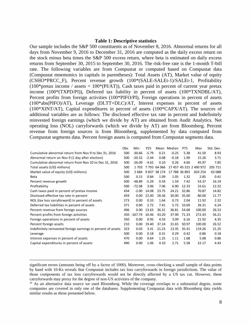
Table 1: Descriptive statistics

Our sample includes the S&P 500 constituents as of November 8, 2016. Abnormal returns for all

days from November 9, 2016 to December 31, 2016 are computed as the daily excess return on

the stock minus beta times the S&P 500 excess return, where beta is estimated on daily excess

returns from September 30, 2015 to September 30, 2016. The risk-free rate is the 1-month T-bill

rate. The following variables are from Compustat or computed based on Compustat data

(Compustat mnemonics in capitals in parentheses): Total Assets (AT), Market value of equity

(CSHO*PRCC_F), Percent revenue growth (100*(SALE-SALEt-1)/SALEt-1, Profitability

(100*pretax income / assets = 100*(PI/AT)), Cash taxes paid in percent of current year pretax

income (100*(TXPD/PI)), Deferred tax liability in percent of assets (100*TXNDBL/AT),

Percent profits from foreign activities (100*PIFO/PI), Foreign operations in percent of assets

(100*abs(PIFO)/AT), Leverage (DLTT+DLC)/AT, Interest expenses in percent of assets

(100*XINT/AT), Capital expenditures in percent of assets (100*CAPX/AT). The sources of

additional variables are as follows: The disclosed effective tax rate in percent and Indefinitely

reinvested foreign earnings (which we divide by AT) are obtained from Audit Analytics. Net

operating loss (NOL) carryforwards (which we divide by AT) are from Bloomberg. Percent

revenue from foreign sources is from Bloomberg, supplemented by data computed from

Compustat segments data. Percent foreign assets is computed from Compustat segments data.

significant errors (amounts being off by a factor of 1000). Moreover, cross-checking a small sample of data points

by hand with 10-Ks reveals that Compustat includes tax loss carryforwards in foreign jurisdictions. The value of

those components of tax loss carryforwards would not be directly affected by a US tax cut. However, these

carryforwards may proxy for the degree of non-US activities of the company. 10 As an alternative data source we used Bloomberg. While the coverage overlaps to a substantial degree, some

companies are covered in only one of the databases. Supplementing Compustat data with Bloomberg data yields

similar results as those presented below.

Obs Min P25 Mean Median P75 Max Std. Dev.

Cumulative abnormal return from Nov 9 to Dec 31, 2016 500 -30.66 -5.79 0.21 -0.25 5.38 41.50 8.93

Abnormal return on Nov 9 (1 day after election) 500 -20.32 -2.04 0.08 -0.18 1.99 15.26 3.71

Cumulative abnormal return from Nov 10 to Dec 31, 2016 500 -26.09 -4.62 0.10 0.26 4.60 45.97 7.85

Total assets (US$ millions) 500 1 703 7 793 64 066 17 457 45 315 2 490 972 205 721

Market value of equity (US$ millions) 500 2 684 9 837 38 174 17 788 36 893 603 254 63 088

Beta 500 0.15 0.84 1.09 1.05 1.32 2.85 0.41

Percent revenue growth 500 -48.89 -5.29 0.59 1.59 7.42 53.37 16.19

Profitability 500 -72.08 3.06 7.06 6.90 12.33 33.61 12.32

Cash taxes paid in percent of pretax income 434 -2.00 14.08 23.75 24.21 32.86 70.87 14.82

Disclosed effective tax rate in percent 459 0.00 22.00 28.36 30.00 35.00 80.00 11.77

NOL (tax loss carryforward) in percent of assets 273 0.00 0.33 1.64 0.73 2.04 11.92 2.32

Deferred tax liabilities in percent of assets 371 0.00 2.72 7.41 5.72 10.69 26.31 6.24

Percent revenue from foreign sources 406 0.00 13.63 36.31 36.81 54.68 100.00 26.53

Percent profits from foreign activities 350 -167.74 10.46 43.20 37.90 71.33 272.43 56.21

Foreign operations in percent of assets 350 0.00 0.95 4.33 3.09 6.16 21.92 4.35

Percent foreign assets 210 0.00 19.40 37.24 31.65 50.97 100.00 26.52

Indefinitely reinvested foreign earnings in percent of assets 323 0.03 3.31 21.23 13.35 35.41 119.26 21.25

Leverage 500 0.00 0.18 0.31 0.29 0.42 0.86 0.18

Interest expenses in percent of assets 470 0.00 0.64 1.25 1.11 1.68 5.08 0.86

Capital expenditures in percent of assets 490 0.00 1.06 4.10 2.71 5.58 22.17 4.43

9

We obtain the percentage of firm revenue from foreign sources from Bloomberg, and we

supplement these data with information from Compustat geographical segment data. Percent

foreign profits is from Compustat. As a proxy for production costs incurred abroad, we compute

the percentage of non-US assets in total assets from Compustat geographical segment data. As

for many companies, this variable is not yet available for 2016; we use data for the years 2013,

2014, and 2015. There are some missing data on foreign revenues, foreign profits, and/or foreign

assets. From Audit Analytics, we obtain data for indefinitely reinvested foreign earnings as of

May 2016, and we divide this number by total assets to obtain our proxy for cash held abroad.

All other variables are standard. Table 1 provides the details of the computation. All explanatory

variables (except market cap) are winsorized at the 1% and 99% levels.

4 Stock return reactions to Trump’s election at the industry level

The most salient feature of reactions of individual stocks to the election – covered also in the

popular press by way of anecdotal evidence, and not controlling for risk – is that President

Trump’s statements about specific industries or groups of industries produced large gains or

losses at the industry level. His promises to deregulate and to discourage imports are, not

surprisingly, strongly reflected in the data. However, as we demonstrate below, initial stock-price

reactions (a) reversed for some industries, and/or (b) did not capture the magnitude of stock price

changes until the end of the year. Presumably, market participants were both digesting the

election and responding to new data available from post-election statements by President-elect

Trump, as well as some from Congress.

Figure 2 plots median abnormal returns in the Fama-French 30 industries between the

market close on November 8 – before the election results were known – and the end of 2016

(light grey), as well as those on the day following the election (dark grey).11 Adjusting for the

market’s overall move, the number of (relative) winners and loser industries is roughly balanced.

The returns for the overall period are in line with what one would expect based on Trump's

statements on the campaign trail: heavy industry (which Trump has promised to resurrect) and

financial firms, which he has said he would deregulate, were perceived to benefit from Trump’s

11 We use medians to avoid the impact of outliers in this detailed industry classification. The picture with average

returns looks very similar. When using Fama-French 17 industries we also obtain the result that steel works, mining,

and drugs benefited most significantly.

10

election. Healthcare, medical equipment, and pharmaceuticals lost dramatically (a consequence

of the expectation that Obamacare would be dismantled or at least significantly altered), as did

textile and apparel firms, reflecting their large dependence on imports, which Trump has vowed

to strongly discourage. Business supplies and shipping containers also lost, probably reflecting

his tough stance on trade.

It is noteworthy that several low-beta industries (beer, tobacco, food products, utilities) are

among the losers, while cyclical industries tend to be among the winners. Presumably,

expectations of higher growth induced investors to rotate from low-risk to high-beta industries.

In a low-growth, low-interest rate environment like the one prevailing in recent years, investors

had been piling into low-beta industries to earn the high dividend yields that they often offer. As

Trump’s election also led to a notable rise in long-term interest rates, stock prices in these

industries suffered.

Figure 2: Median abnormal returns after the election by Fama-French 30 industries

The results in Figure 2 also reveal that the cumulative abnormal returns from the election to

year-end differ substantially from the immediate response after the election, shown in dark grey

in the figure. Apparel and textiles, which are the worst performers during the overall period, only

-10

-8

-6

-4

-2

0

2

4

6

8

10

Ap

pa

rel

Te

xtile

s

Be

er

& L

iqu

or

Pri

ntin

g a

nd

Pu

blish

ing

Re

cre

atio

n

Pe

rso

na

l a

nd

Bu

sin

ess S

erv

ice

s

Bu

sin

ess S

up

plie

s a

nd

Sh

ipp

ing

Co

nta

ine

rs

Fo

od

Pro

du

cts

,He

alth

ca

re,

Me

dic

al E

qu

ipm

en

t

Ph

arm

ace

utica

l P

rod

ucts

Co

nsu

me

r G

oo

ds

Pre

cio

us M

eta

ls,

No

n-M

eta

llic

, a

nd

Ind

ustr

ial M

eta

l M

inin

gC

on

str

uctio

n a

nd

Co

nstr

uctio

n

Ma

teri

als

Utilitie

s

Bu

sin

ess E

qu

ipm

en

t

To

ba

cco

Pro

du

cts

Fa

bri

ca

ted

Pro

du

cts

an

d

Ma

ch

ine

ry

Ch

em

ica

ls

Re

sta

rau

nts

, H

ote

ls,

Mo

tels

Ele

ctr

ica

l E

qu

ipm

en

t

Au

tom

ob

ile

s a

nd

Tru

cks

Wh

ole

sa

le

Pe

tro

leu

m a

nd

Na

tura

l G

as

Eve

ryth

ing

Els

e

Re

tail

Tra

nsp

ort

atio

n

Ste

el W

ork

s E

tc

,Ba

nkin

g,

Insu

ran

ce

, R

ea

l E

sta

te

Tra

din

g

Co

mm

un

ica

tio

n

Air

cra

ft,

sh

ips,

an

d r

ailro

ad

eq

uip

me

nt

Me

dia

n A

bn

orm

al

Re

turn

in

%

CAR from Election to Year-End AR on Nov. 9

z

11

had a modest drop on the day after the election. A similar pattern holds for medical equipment

and medical products: the immediate reaction to Trump's election was one of relief and indeed a

light increase, as markets were seriously worried about Hillary Clinton’s critical stance on drug

prices. However, concerns about the industry's profitability escalated when Trump started

making critical statements about pharmaceutical products’ prices after the election.12 At the other

end of the spectrum, markets seem to have been initially too optimistic about the prospects for

the steel industry (which had been one of the hot spots of the campaign), and barely reacted at

the outset to the prospect of deregulation in the financial industry. Another interesting case is the

automobile industry, which suffered initially (probably reflecting fears of Trump's meddling in

plant location decisions), but had become one of the top performers by year-end (probably

reflecting expectations of higher profits due to tariffs on imports).

Thus, while the initial strongly positive response of the overall stock and bond market to the

election outcome persisted through the rest of the year, there was no continuation of industry-

level abnormal returns, quite the opposite. As can be seen in Figure 3, the relationship between

the abnormal returns on November 9 and those between November 10 and year-end at the

industry level is actually negative (the correlation is –0.25).

This finding has two potential explanations. The first is that investors overreacted to the

initial news. What speaks against this interpretation is that at the overall market level – both for

stocks and bonds yields – the response on the day following the election continued into year-end

(and indeed through the Inauguration on January 20, 2017). Thus, for the observed phenomenon

to arise, one would need investors to overreact about the prospects for some industries and

underreact about the prospects for others, an unlikely parlay. The second, and more plausible,

explanation is that the market’s assessment about the strength and/or likelihood of some of the

incoming administration’s future policies changed after the election or took more time to be

incorporated into prices because processing the information on these policies was more difficult.

What speaks in favor of this latter interpretation are the strong negative returns until the end of

the year in import-intensive and trade-sensitive industries (textile, shipping containers), and the

12 Considering the abnormal returns using the Fama-French 48 industries, in which healthcare and pharmaceuticals

constitute two different industries, provides support for this interpretation. In this case, the abnormal returns on the

day after the election are +5.02% for pharmaceuticals and -4.71% for healthcare, while the cumulative abnormal

returns from the election to the end of the year are -3.95% for pharmaceuticals and -2.34% for healthcare.

12

positive returns in industries that would benefit from trade restrictions (automobiles) or proposed

deregulation (banking).

While these descriptive industry-level results reveal large differences in the asset price

response across industries, heterogeneity across firms within the same industry is typically as

large as that across industries, both in terms of abnormal returns and firm characteristics. Below,

we capitalize on firm-level heterogeneity in order to assess the impact of different prospective

policy developments. Since our analysis reveals large differences between the immediate

response to the election and that through year-end, we investigate these responses separately.

Figure 3: Relationship between median abnormal returns on November 9, 2016 and from

November 10 to year-end 2016 by Fama-French 30 industries

5 Explaining the cross-section of stock return reactions

This section investigates the cross-section of stock price responses to the election outcome. It

examines the impact of expectations about overall growth, taxation, and trade policy.

5.1 Growth expectations

If the market believes that Trump is good for the aggregate economy, those companies that are

more strongly exposed to the (US) economy will do better. To have a first look at this

hypothesis, Figure 4 presents a binned scatter plot. That is, all stocks are sorted into 20 equal-

-10

-50

5

Ab

no

rmal R

etu

rn N

ov. 10

- D

ec. 3

1

-5 0 5 10Abnormal Return Nov. 9

13

sized bins by their market beta, and we then compute the average abnormal stock return in each

of the bins.

A positive relationship emerges. Clearly, investors flocked to high-beta equities after the

election. This result adds to the insights of Figure 2. There, we had seen that many of the worst

performing industries were low-beta industries. However, note that Figure 4 shows results

controlling not only for market beta (via the abnormal return computation), but also for industry

fixed effects.

Figure 4: Binned scatter plots of Beta against abnormal returns from November 9 to

December 31, 2016 (left panel) and abnormal returns on November 9, 2016 (right panel)

(controlling for Fama-French 30 industries fixed effects)

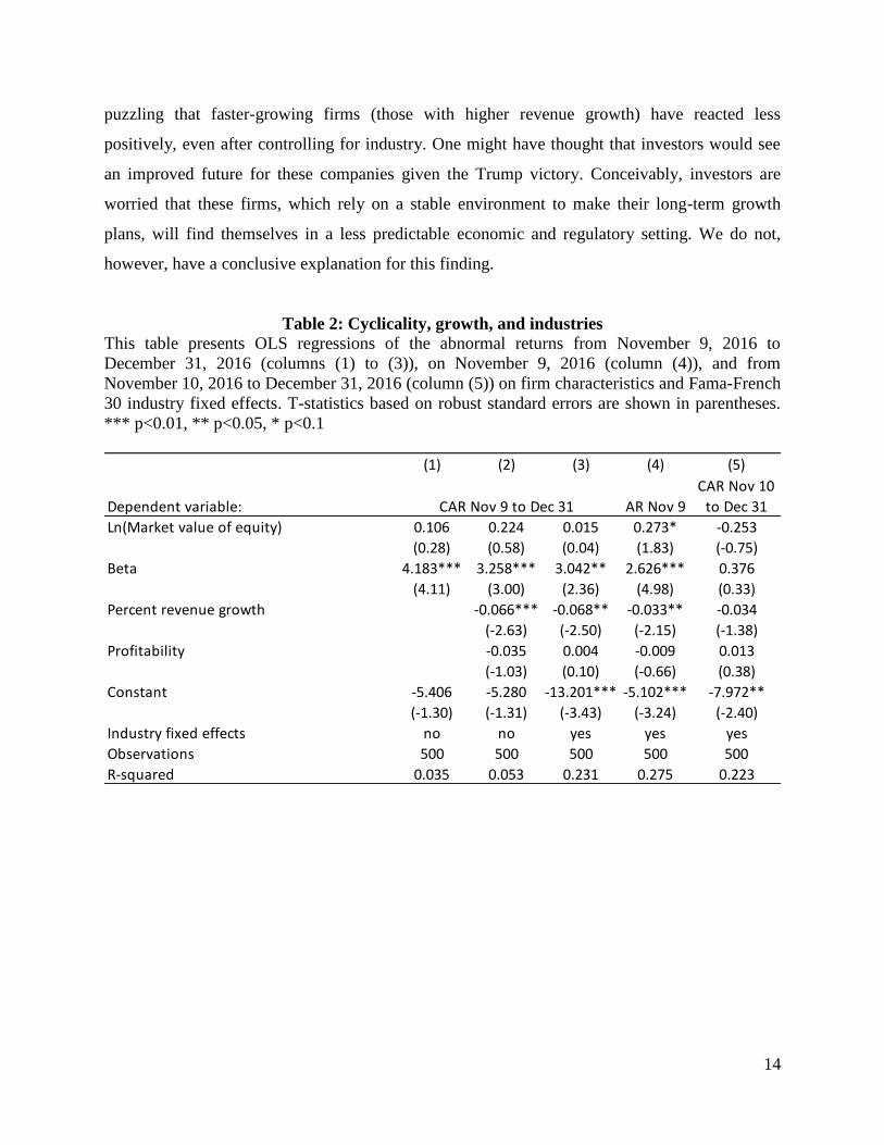
Table 2 presents the corresponding regression output, documenting strong statistical

significance of the positive market reaction of high-beta stocks. Strikingly, almost all of this

reaction took place on the first day, while beta does not significantly predict abnormal returns

into year-end. While we do not report the coefficients on the industry dummies for space

reasons, this regression analysis shows that the industry fixed effects that are significant without

controlling for beta remain significant (with one exception) even when controlling for beta. This

suggests that some industries were expected to benefit over and above what the aggregate

economy does, even after adjusting for their average cyclicality.

Table 2 also reveals that size does not seem to matter directly for firms’ stock market

performance. Profitability itself does not explain abnormal returns either. Thus, the market does

not seem to believe that CEO Trump would “fire” weakly performing firms. It is somewhat

-4-3

-2-1

01

23

45

6

Perc

ent a

bn

orm

al re

turn

s fro

m N

ov 9

to

Dec 3

1

.5 1 1.5 2Beta

-4-3

-2-1

01

23

45

6

Perc

ent a

bn

orm

al re

turn

s o

n N

ov 9

.5 1 1.5 2Beta

14

puzzling that faster-growing firms (those with higher revenue growth) have reacted less

positively, even after controlling for industry. One might have thought that investors would see

an improved future for these companies given the Trump victory. Conceivably, investors are

worried that these firms, which rely on a stable environment to make their long-term growth

plans, will find themselves in a less predictable economic and regulatory setting. We do not,

however, have a conclusive explanation for this finding.

Table 2: Cyclicality, growth, and industries

This table presents OLS regressions of the abnormal returns from November 9, 2016 to

December 31, 2016 (columns (1) to (3)), on November 9, 2016 (column (4)), and from

November 10, 2016 to December 31, 2016 (column (5)) on firm characteristics and Fama-French

30 industry fixed effects. T-statistics based on robust standard errors are shown in parentheses.

*** p<0.01, ** p<0.05, * p<0.1

(1) (2) (3) (4) (5)

Dependent variable: AR Nov 9

CAR Nov 10

to Dec 31

Ln(Market value of equity) 0.106 0.224 0.015 0.273* -0.253

(0.28) (0.58) (0.04) (1.83) (-0.75)

Beta 4.183*** 3.258*** 3.042** 2.626*** 0.376

(4.11) (3.00) (2.36) (4.98) (0.33)

Percent revenue growth -0.066*** -0.068** -0.033** -0.034

(-2.63) (-2.50) (-2.15) (-1.38)

Profitability -0.035 0.004 -0.009 0.013

(-1.03) (0.10) (-0.66) (0.38)

Constant -5.406 -5.280 -13.201*** -5.102*** -7.972**

(-1.30) (-1.31) (-3.43) (-3.24) (-2.40)

Industry fixed effects no no yes yes yes

Observations 500 500 500 500 500

R-squared 0.035 0.053 0.231 0.275 0.223

CAR Nov 9 to Dec 31

15

5.2 Corporate tax rates

While the details of any future tax plan remain somewhat hazy, it is clear that President Trump

wants to cut corporate taxes significantly below their current 35% level, and is very likely to

succeed, given that the Republican majority in Congress, as well as many Democratic legislators,

have the same preference. Had Hillary Clinton won the election, corporate taxes might well have

been trimmed, but not cut nearly to the level that Trump has proposed, namely 15%. (President

Obama had supported a cut to 28%.)

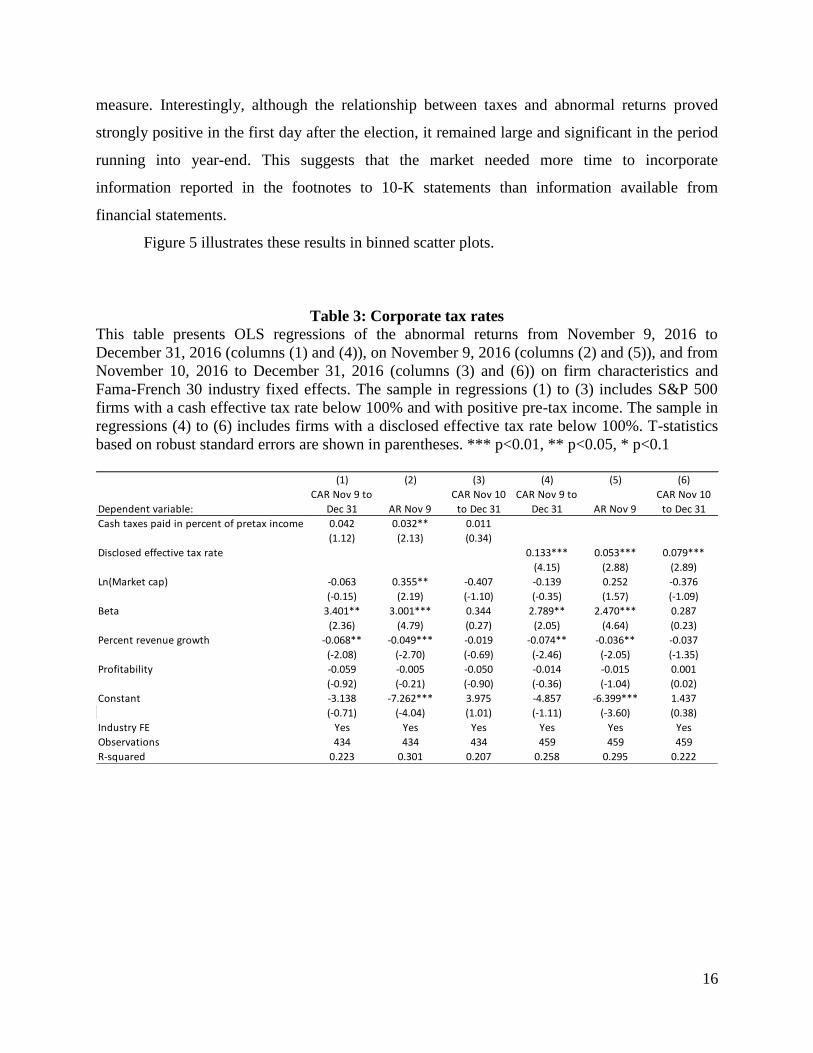
Given the surprisingly large expected reduction in corporate taxes due to Trump’s

election, we would expect those companies currently paying higher taxes to perform better. At

first sight, Column (1) of Table 3 appears to suggest only a modest (and statistically

insignificant) relationship between the cash effective tax rate and the cumulative abnormal

returns from November 9, 2016 to December 31, 2016. Here, one needs to keep in mind that

long-term returns are notoriously difficult to predict and noisy. However, as can be seen in

Column (2), there was actually a strong market response to differences in taxation across firms,

but it took place swiftly on the first day after the election. Economically, this effect is sizable: In

this sample, the standard deviation of the cash effective tax rate is 15.4. Therefore, a one

standard deviation higher effective tax rate is associated with a 0.41 percentage point

(15.4*0.032) increase in the abnormal return on the day after the election, more than 10% of a

standard deviation of the abnormal returns. A substantial portion of the overall reaction was,

therefore, already impounded in stock prices on the first day. Tables available on request show

that controlling for special items does not affect the results.13

Columns (4) to (6) of Table 3 use the disclosed effective tax rate instead of the cash ETR.

This item, reported in the tax footnotes to 10-K statements of most, though not all companies,

captures the total tax expenses (rather than the cash taxes) that a company records. We again find

a more positive investor reaction for those firms with a higher tax burden according to this

13 As a measure of the level of a firm’s tax sheltering, we also compute the book tax gap following Manzon and

Plesko (2002) and Jalan, Kale and Meneghetti (2016). This captures the difference between the income a firm

reports to its shareholders based on GAAP and the one it reports to the income tax authorities based on tax laws. The

latter is not observable. Following the literature, we compute [PI-PIFO-TXFED/0.35] – TXS – TXO – ESUBC. The

part in the square brackets is the “unadjusted spread”. The three items subtracted at the end (state income taxes,

other income taxes, unremitted earnings in non-consolidated subsidiaries) can affect the gap for reasons unrelated to

tax sheltering. Dividing the total quantity of the above calculation by total assets yields the book tax gap. We do not

find a significant association of this proxy for tax sheltering and announcement returns. However, the sample in this

is quite small (around 200 observations) due to missing data (which, according to Manzon and Plesko (2002), should

not be treated as zero entries in these cases).

16

measure. Interestingly, although the relationship between taxes and abnormal returns proved

strongly positive in the first day after the election, it remained large and significant in the period

running into year-end. This suggests that the market needed more time to incorporate

information reported in the footnotes to 10-K statements than information available from

financial statements.

Figure 5 illustrates these results in binned scatter plots.

Table 3: Corporate tax rates


December 31, 2016 (columns (1) and (4)), on November 9, 2016 (columns (2) and (5)), and from

November 10, 2016 to December 31, 2016 (columns (3) and (6)) on firm characteristics and

Fama-French 30 industry fixed effects. The sample in regressions (1) to (3) includes S&P 500

firms with a cash effective tax rate below 100% and with positive pre-tax income. The sample in

regressions (4) to (6) includes firms with a disclosed effective tax rate below 100%. T-statistics

based on robust standard errors are shown in parentheses. *** p<0.01, ** p<0.05, * p<0.1

(1) (2) (3) (4) (5) (6)

Dependent variable:

CAR Nov 9 to

Dec 31 AR Nov 9

CAR Nov 10

to Dec 31

CAR Nov 9 to

Dec 31 AR Nov 9

CAR Nov 10

to Dec 31

Cash taxes paid in percent of pretax income 0.042 0.032** 0.011

(1.12) (2.13) (0.34)

Disclosed effective tax rate 0.133*** 0.053*** 0.079***

(4.15) (2.88) (2.89)

Ln(Market cap) -0.063 0.355** -0.407 -0.139 0.252 -0.376

(-0.15) (2.19) (-1.10) (-0.35) (1.57) (-1.09)

Beta 3.401** 3.001*** 0.344 2.789** 2.470*** 0.287

(2.36) (4.79) (0.27) (2.05) (4.64) (0.23)

Percent revenue growth -0.068** -0.049*** -0.019 -0.074** -0.036** -0.037

(-2.08) (-2.70) (-0.69) (-2.46) (-2.05) (-1.35)

Profitability -0.059 -0.005 -0.050 -0.014 -0.015 0.001

(-0.92) (-0.21) (-0.90) (-0.36) (-1.04) (0.02)

Constant -3.138 -7.262*** 3.975 -4.857 -6.399*** 1.437

(-0.71) (-4.04) (1.01) (-1.11) (-3.60) (0.38)

Industry FE Yes Yes Yes Yes Yes Yes

Observations 434 434 434 459 459 459

R-squared 0.223 0.301 0.207 0.258 0.295 0.222

17

Figure 5: Binned scatter plots of Cash effective tax rate (top two panels) and Disclosed

effective tax rate (bottom two panels) against abnormal returns from November 9 to

December 31, 2016 (left panels) and abnormal returns on November 9, 2016 (right panels)


Table 4 explores another set of tax-related consequences. On the one hand, firms with substantial

tax loss carryforward balances (accumulated net operating losses, NOLs) should underperform

since a tax cut reduces the present value of the expected tax savings provided by these NOLs. On

the other hand, firms with deferred tax liabilities should benefit: Deferred tax liabilities are future

taxes payable, and if future tax rates are expected to be lower, the present value of these

liabilities is reduced, implying a higher firm value. Table 4 shows that the market reacted in line

with these predicted effects, and that the reaction occurred immediately after the election.

In sum, these results show not only that the market reacted in the expected way to

Trump’s election, but this relatively clean natural experiment also confirms that taxes are a very

important component of firm value.

-3-2

-10

12

34

Perc

ent a

bn

orm

al re

turn

s fro

m N

ov 9

to

Dec 3

1

0 20 40 60Cash effective tax rate in percent

-3-2

-10

12

34

Perc

ent a

bn

orm

al re

turn

s o

n N

ov 9

0 20 40 60Cash effective tax rate in percent

-4-3

-2-1

01

23

45

6

Perc

ent a

bn

orm

al re

turn

s fro

m N

ov 9

to

Dec 3

1

0 20 40 60Disclosed effective tax rate in percent

-4-3

-2-1

01

23

45

6

Perc

ent a

bn

orm

al re

turn

s o

n N

ov 9

0 20 40 60Disclosed effective tax rate in percent

18

Table 4: Loss carryforwards and deferred tax liabilities




Fama-French 30 industry fixed effects. T-statistics based on robust standard errors are shown in

parentheses. *** p<0.01, ** p<0.05, * p<0.1

5.3 Foreign operations

It is not clear a priori whether stocks oriented towards the US economy will fare better or worse

than those that are more exposed to the world economy.

On the one hand, there are several arguments favoring stocks with a domestic focus.

First, market participants may simply have higher expectations for US growth versus foreign

growth. Second, stocks active abroad are more subject to the risk of trade wars that bring

retaliation by other countries. In either case, firms with larger foreign presence would do worse.

(Without further evidence, one cannot distinguish between the two explanations.) Third, Trump’s

infrastructure plan would naturally benefit domestically-focused firms. Fourth, Trump’s

expansionist fiscal policies and the associated increase in inflation expectations are likely to

foster Fed rate hikes. In a number of speeches following the election, Federal Reserve officials

(1) (2) (3) (4) (5) (6)

Dependent variable:

CAR Nov 9 to

Dec 31 AR Nov 9

CAR Nov 10

to Dec 31

CAR Nov 9 to

Dec 31 AR Nov 9

CAR Nov 10

to Dec 31

NOL carryforwards in percent of assets -0.495 -0.226** -0.281

(-1.62) (-2.11) (-1.13)

Deferred tax liability in percent of assets 0.080 0.134*** -0.049

(0.58) (2.73) (-0.41)

Cash taxes paid in percent of pretax income -0.027 0.020 -0.043 0.039 0.026 0.014

(-0.44) (0.92) (-0.77) (0.89) (1.52) (0.39)

Ln(Market cap) -0.136 0.389* -0.497 -0.197 0.324 -0.509

(-0.23) (1.68) (-0.98) (-0.39) (1.65) (-1.15)

Beta 3.930* 3.067*** 0.893 2.926 3.376*** -0.411

(1.66) (3.08) (0.45) (1.61) (4.10) (-0.26)

Percent revenue growth -0.123*** -0.062** -0.061* -0.080** -0.053** -0.025

(-2.74) (-2.40) (-1.70) (-2.13) (-2.45) (-0.82)

Profitability -0.130 -0.028 -0.097 -0.052 0.021 -0.067

(-1.14) (-0.85) (-1.00) (-0.64) (0.66) (-0.96)

Constant -0.380 -6.682** 5.818 -2.349 -8.538*** 5.885

(-0.06) (-2.46) (0.99) (-0.43) (-3.87) (1.24)


Observations 240 240 240 329 329 329

R-squared 0.260 0.302 0.248 0.190 0.300 0.201

19

made no secret that they might tighten policy faster if fiscal policy became more expansionary.14

While higher inflation per se would hurt the dollar in the long-run, the rate hikes could initially

strengthen it, hurting exporters. Indeed, the ICE US Dollar index appreciated by 4.44% between

November 8 and year-end, while the expected path of the Federal Funds rate implied from Fed

Fund futures prices steepened.15 According to the minutes of the December 2016 FOMC

meeting, “[s]urveys of market participants had indicated that revised expectations for

government spending and tax policy following the U.S. elections in early November were seen as

the most important reasons, among several factors, for the increase in longer-term Treasury

yields, the climb in equity valuations, and the rise in the dollar.” At that same meeting, the

median of FOMC participants’ projections for GDP growth rose, but only slightly. Furthermore,

“[t]hose increasing their projections for output growth in those years cited expected changes in

fiscal, regulatory, or other policies as factors contributing to their revisions. However, many

participants noted that the effects on the economy of such policy changes, if implemented, would

likely be partially offset by tighter financial conditions, including higher longer-term interest

rates and a strengthening of the dollar.”

On the other hand, the House Republicans’ tax plan (Republicans 2016) has been

interpreted to help make US companies more competitive abroad. If so, that would (relatively)

favor internationally-oriented stocks. While the exact implementation is not known to date, the

basic gist of the plan is that US companies would not pay tax on profits earned on overseas sales

anymore. Conversely, products, services and intangibles that are imported will be subject to US

tax regardless of where they are produced.16 (See Tax Foundation (2016) for a description of the

plan.) The Tax Foundation, however, dismisses the argument that exporters would benefit from

the plan. They write: “Of course, U.S. producers may think of this as a subsidy for exports

because they would not be taxed on sales overseas. But if businesses were able to reduce the

prices of their goods they sell overseas due to the border adjustment, this would trigger a higher

14 The minutes of the December 2016 FOMC meeting, which were released on January 4, 2017, are in line with

these statements made by Fed officials before year-end. The minutes state: «Many participants noted that there was

currently substantial uncertainty about the size, composition, and timing of prospective fiscal policy changes, but

they also commented that a more expansionary fiscal policy might raise aggregate demand above sustainable levels,

potentially necessitating somewhat tighter monetary policy than currently anticipated.» 15 On November 8, futures markets viewed the most likely range of the Fed Funds target rate following the

December 2017 FOMC meeting to be 0.5-0.75% or 0.75%-1% (with both outcomes about equally likely). At the end

of the year, the most likely range according to futures prices was 1-1.25%. 16 Another aspect of tax policy is the tax treatment of profits made by US firms’ foreign subsidiaries. We consider

this aspect at the end of this section.

20

demand for dollars in order to purchase those goods. This higher demand for dollars would

increase the value of the dollar relative to foreign currencies and offset any perceived trade

advantage granted by the border adjustment.” In line with this view, some market observers

have claimed that (expectations of) the plan’s enactment would lead to a strong appreciation of

the dollar. Since some version of the plan appears likely to succeed, this raises the question why

the dollar has not appreciated more strongly during the period.

Summarizing, the proposed policies could have both advantages and disadvantages for

exporters and firms with significant foreign operations, and it is not obvious which would

predominate.17 But investors through the stock market did take a view. Table 5 and Figure 6

suggest that investors strongly believed that domestically-oriented companies would have a

relative advantage: abnormal returns are significantly negatively related to the fraction of

revenues being earned outside the US. Interestingly, the negative relationship between foreign

revenue and stock returns was strong not only on the day following the election, but persisted

into year-end. A potential explanation is that two effects underlie the observed returns. The first

– faster US GDP growth – was recognized early on by markets, while the second – negative

spillover effects from more restrictive trade policies – needed some time to be incorporated into

prices.

It is worth noting that the effects in Table 5 are quantitatively important. For example, a

one standard deviation increase in the fraction of foreign revenues is associated with a 0.96

percentage point lower first-day return, a quarter of a standard deviation of these returns, and

with a 2.15 percentage point lower cumulative abnormal return through year-end, again around a

quarter of a standard deviation of these returns.

17 Analysts tend to see advantages for domestic stocks. For example, in a note released on November 9, 2016 (and

reported on zerohedge.com), Goldman Sachs chief strategist David Kostin argued that domestic stocks will do better

than foreign-exposed stocks (Kostin 2016).

21

Figure 6: Binned scatter plot of Percent foreign revenues against abnormal returns from

November 9 to December 31, 2016 (left panel) and abnormal returns on November 9, 2016

(right panel)


Table 5: Foreign operations, part 1


December 31, 2016 (column (1)), on November 9, 2016 (column (2)), and from November 10,

2016 to December 31, 2016 (column (3)) on firm characteristics and Fama-French 30 industry

fixed effects. T-statistics based on robust standard errors are shown in parentheses. *** p<0.01,

** p<0.05, * p<0.1

-4-3

-2-1

01

23

4

Perc

ent a

bn

orm

al re

turn

s fro

m N

ov 9

to

Dec 3

1

0 20 40 60 80 100Percent foreign revenues

-4-3

-2-1

01

23

4

Perc

ent a

bn

orm

al re

turn

s o

n N

ov 9

0 20 40 60 80 100Percent foreign revenues

(1) (2) (3)

Dependent variable:

CAR Nov 9 to

Dec 31 AR Nov 9

CAR Nov 10 to

Dec 31

Percent revenue from foreign sources -0.080*** -0.036*** -0.044**

(-3.36) (-4.19) (-2.10)

Cash taxes paid in percent of pretax income 0.012 0.038** -0.024

(0.31) (2.36) (-0.70)

Ln(Market value of equity) 0.285 0.596*** -0.296

(0.61) (3.56) (-0.70)

Beta 3.914** 3.152*** 0.698

(2.16) (4.46) (0.44)

Percent revenue growth -0.079** -0.065*** -0.016

(-2.05) (-3.23) (-0.51)

Profitability -0.015 0.012 -0.026

(-0.23) (0.51) (-0.44)

Constant -4.881 -9.006*** 3.974

(-1.01) (-4.74) (0.89)

Industry FE

Observations 354 354 354

R-squared 0.246 0.337 0.227

22

Table 6: Foreign operations, part 2


December 31, 2016 (column (1)), on November 9, 2016 (column (2)), and from November 10,

2016 to December 31, 2016 (column (3)) on firm characteristics and Fama-French 30 industry

fixed effects. T-statistics based on robust standard errors are shown in parentheses. *** p<0.01,

** p<0.05, * p<0.1

(1) (2) (3)

Dependent variable:

CAR Nov 9 to

Dec 31 AR Nov 9

CAR Nov 10 to

Dec 31

Panel A

Percent profits from foreign activities -0.043** -0.012* -0.031**

(-2.57) (-1.72) (-2.16)

Cash taxes paid in percent of pretax income 0.042 0.032* 0.011

(0.90) (1.91) (0.28)


R-squared 0.233 0.313 0.196

Panel B

Foreign operations in percent of assets -0.494*** -0.134** -0.364***

(-3.51) (-2.05) (-3.09)

Cash taxes paid in percent of pretax income 0.022 0.025 -0.002

(0.50) (1.55) (-0.06)


R-squared 0.232 0.297 0.211

Panel C

Percent foreign assets -0.008 -0.004 -0.003

(-0.33) (-0.48) (-0.13)

Cash taxes paid in percent of pretax income -0.023 0.047** -0.066

(-0.38) (2.34) (-1.10)


R-squared 0.230 0.438 0.243

Panel D

Indefinitely reinvested foreign earnings in percent of assets -0.070** -0.029** -0.040

(-2.30) (-2.14) (-1.50)

Cash taxes paid in percent of pretax income 0.016 0.019 0.001

(0.32) (0.98) (0.02)


R-squared 0.241 0.317 0.211

All panels

Constant Yes Yes Yes

Control variables (Size, beta, sales growth, profitability) Yes Yes Yes

Industry FE Yes Yes Yes

23

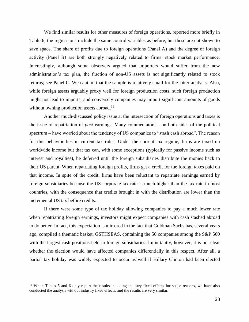
We find similar results for other measures of foreign operations, reported more briefly in

Table 6; the regressions include the same control variables as before, but these are not shown to

save space. The share of profits due to foreign operations (Panel A) and the degree of foreign

activity (Panel B) are both strongly negatively related to firms’ stock market performance.

Interestingly, although some observers argued that importers would suffer from the new

administration’s tax plan, the fraction of non-US assets is not significantly related to stock

returns; see Panel C. We caution that the sample is relatively small for the latter analysis. Also,

while foreign assets arguably proxy well for foreign production costs, such foreign production

might not lead to imports, and conversely companies may import significant amounts of goods

without owning production assets abroad.18

Another much-discussed policy issue at the intersection of foreign operations and taxes is

the issue of repatriation of past earnings. Many commentators – on both sides of the political

spectrum – have worried about the tendency of US companies to “stash cash abroad”. The reason

for this behavior lies in current tax rules. Under the current tax regime, firms are taxed on

worldwide income but that tax can, with some exceptions (typically for passive income such as

interest and royalties), be deferred until the foreign subsidiaries distribute the monies back to

their US parent. When repatriating foreign profits, firms get a credit for the foreign taxes paid on

that income. In spite of the credit, firms have been reluctant to repatriate earnings earned by

foreign subsidiaries because the US corporate tax rate is much higher than the tax rate in most

countries, with the consequence that credits brought in with the distribution are lower than the

incremental US tax before credits.

If there were some type of tax holiday allowing companies to pay a much lower rate

when repatriating foreign earnings, investors might expect companies with cash stashed abroad

to do better. In fact, this expectation is mirrored in the fact that Goldman Sachs has, several years

ago, compiled a thematic basket, GSTHSEAS, containing the 50 companies among the S&P 500

with the largest cash positions held in foreign subsidiaries. Importantly, however, it is not clear

whether the election would have affected companies differentially in this respect. After all, a

partial tax holiday was widely expected to occur as well if Hillary Clinton had been elected

18 While Tables 5 and 6 only report the results including industry fixed effects for space reasons, we have also

conducted the analysis without industry fixed effects, and the results are very similar.

24

President.19 Accordingly, the market reaction to the election on that count would be driven not so

much by the enactment of a tax holiday as such, but by the perceived difference in the holiday

tax rate between the two candidates, with Trump likely to favor a lower rate than Clinton. Panel

D of Table 6 shows, however, that companies with large cash holdings in foreign subsidiaries in

fact responded worse to the Trump election. When controlling for foreign revenues (not shown),

the effect is insignificant, suggesting that foreign cash holdings at least partly proxy for a firm’s

foreign activities overall.

Recall that we found above that companies with a lot of business abroad – which are

more likely to be the ones holding cash abroad – actually responded worse to Trump’s election.

Thus, if the repatriation tax holiday is implicitly at play in the market’s expectations, something

else must be particularly bad for firms with foreign activities.

5.4 Interest expense deductibility and capital investment expensing

Another approach that has been proposed to make the US more competitive is to strengthen

firms’ incentives to invest. Specifically, under the House Republicans’ tax plan, businesses

would no longer need to depreciate capital investments. Instead, they will be able to expense

them fully in the period that they are made. Thus, firms would be able to defer corporate income

taxes, which should have a positive effect on stock prices, with a larger effect for firms making

greater capital expenditures relative to their size. In order to avoid a tax subsidy for debt-

financed investment, the House Republicans’ plan would no longer allow net interest expenses to

be deducted. This would hurt those firms with more leverage (which generates value through the

tax shield in place up to now) and those with greater proportional interest expenses.

Columns (1), (3), and (5) of Table 7 reveal a negative but insignificant relationship

between firm leverage and abnormal returns in the full specification.20 However, firms with

substantial interest expenses reacted more negatively, as seen in column (2) of Table 7, though

the reaction did not come immediately after the election (columns (4) and (6)). This result is

illustrated in the top panel of Figure 7. This result may not reflect an expectation regarding

19 A different, but related question is what companies would do with the repatriated cash. Despite explicit

prohibitions against the use of repatriated cash for repurchases, it appears that this is exactly what companies did use

this cash for after the 2004 tax holiday (Dharmapala, Foley and Forbes 2011). Thus, an indirect effect leading to

differential stock market reactions to repatriation could be due to differences in firms’ financial constraints. 20 The correlation between leverage and beta in our sample is slightly negative but statistically insignificant. There is

no significant relationship between abnormal returns and leverage even if we do not control for beta. However, there

is a negative relationship between leverage and abnormal returns when not controlling for foreign revenues.

25

interest deductibility being abolished, as deductions also lose value when taxes are slashed (as

the market seems to expect; see Section 5.2).

Table 7: Interest expense deductibility and expensing of capital expenditures




Fama-French 30 industry fixed effects. T-statistics based on robust standard errors are shown in

parentheses. *** p<0.01, ** p<0.05, * p<0.1

We find no significant relationship between immediate or long-run abnormal returns and

CAPEX, as can also be seen by the virtually flat regression lines in the bottom panel of Figure 7.

(We control for leverage or interest expenses in these regressions, as any benefit from immediate

expensing would be offset to some extent from the non-deductibility of interest, assuming the

investments would have been financed with bonds, but the same result holds when not

controlling for these variables.) Thus, investors seemed to believe that either the Republicans’

(1) (2) (3) (4) (5) (6)

Dependent variable:

Leverage -1.974 -0.437 -1.411

(-0.62) (-0.38) (-0.51)

Interest expenses in percent of assets -1.488** -0.206 -1.248**

(-2.24) (-0.69) (-2.30)

Capital expenditures in percent of assets 0.035 0.128 -0.020 0.004 0.035 0.103

(0.16) (0.55) (-0.22) (0.04) (0.20) (0.55)

Cash taxes paid in percent of pretax income 0.009 -0.021 0.038** 0.032** -0.027 -0.051

(0.23) (-0.53) (2.35) (1.99) (-0.75) (-1.40)

Percent revenue from foreign sources -0.080*** -0.076*** -0.036*** -0.035*** -0.044** -0.041*

(-3.40) (-3.19) (-4.31) (-4.03) (-2.11) (-1.95)

Ln(Market value of equity) 0.274 0.026 0.582*** 0.609*** -0.292 -0.558

(0.57) (0.06) (3.36) (3.17) (-0.67) (-1.39)

Beta 3.829** 3.270* 3.099*** 3.053*** 0.686 0.203

(2.09) (1.76) (4.45) (4.01) (0.42) (0.12)

Revenue growth rate -0.080** -0.094** -0.065*** -0.066*** -0.017 -0.029

(-2.06) (-2.41) (-3.19) (-3.28) (-0.56) (-0.92)

Profitability -0.029 -0.084 0.011 -0.002 -0.037 -0.080

(-0.44) (-1.49) (0.44) (-0.06) (-0.63) (-1.60)

Constant -3.995 0.893 -8.587*** -8.590*** 4.422 9.203*

(-0.72) (0.16) (-4.02) (-3.59) (0.88) (1.93)


Observations 352 341 352 341 352 341

R-squared 0.248 0.263 0.336 0.342 0.230 0.244

CAR Nov 9 to Dec 31 AR Nov 9 CAR Nov 10 to Dec 31

26

proposed capital expenditure rule is unlikely to have large effects, or that it is unlikely to be

implemented.21

Figure 7: Binned scatter plots of Interest expense in percent of assets (top two panels) and

Capital expenditures in percent of assets (bottom two panels) against abnormal returns

from November 9 to December 31, 2016 (left panels) and abnormal returns on November 9,

2016 (right panels)


21 While the House Republicans’ plan removes interest deductibility for all firms and allows all firms to expense

capital investments, Trump’s plan, as described on https://www.donaldjtrump.com/policies/tax-plan/ (visited on

February 1, 2017), is to restrict the possibility to expense capital investment to manufacturers. These companies

would be allowed to opt (once in three years) to expense, but would then give up the interest deduction. When

restricting the sample to the 165 firms in SIC codes 2000 to 3999 (manufacturing), the coefficient on capital

expenditures is positive in regressions like those in Table 7, but still below conventional significance levels.

-4-3

-2-1

01

23

4

Perc

ent a

bn

orm

al re

turn

s fro

m N

ov 9

to

Dec 3

1

0 1 2 3 4Interest expense in percent of total assets

-4-3

-2-1

01

23

4

Perc

ent a

bn

orm

al re

turn

s o

n N

ov 9

0 1 2 3 4Interest expense in percent of total assets

-4-3

-2-1

01

23

4

Perc

ent a

bn

orm

al re

turn

s fro

m N

ov 9

to

Dec 3

1

-5 0 5 10 15Capital expenditures in percent of total assets

-4-3

-2-1

01

23

4

Perc

ent a

bn

orm

al re

turn

s o

n N

ov 9

-5 0 5 10 15Capital expenditures in percent of total assets

https://www.donaldjtrump.com/policies/tax-plan/

27

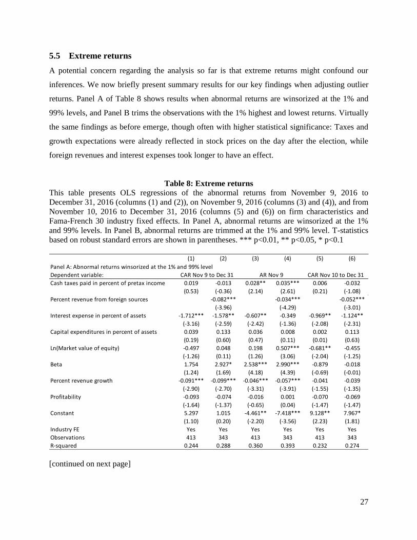
5.5 Extreme returns

A potential concern regarding the analysis so far is that extreme returns might confound our

inferences. We now briefly present summary results for our key findings when adjusting outlier

returns. Panel A of Table 8 shows results when abnormal returns are winsorized at the 1% and

99% levels, and Panel B trims the observations with the 1% highest and lowest returns. Virtually

the same findings as before emerge, though often with higher statistical significance: Taxes and

growth expectations were already reflected in stock prices on the day after the election, while

foreign revenues and interest expenses took longer to have an effect.

Table 8: Extreme returns




Fama-French 30 industry fixed effects. In Panel A, abnormal returns are winsorized at the 1%

and 99% levels. In Panel B, abnormal returns are trimmed at the 1% and 99% level. T-statistics

based on robust standard errors are shown in parentheses. *** p<0.01, ** p<0.05, * p<0.1

[continued on next page]

(1) (2) (3) (4) (5) (6)

Panel A: Abnormal returns winsorized at the 1% and 99% level

Dependent variable:

Cash taxes paid in percent of pretax income 0.019 -0.013 0.028** 0.035*** 0.006 -0.032

(0.53) (-0.36) (2.14) (2.61) (0.21) (-1.08)

Percent revenue from foreign sources -0.082*** -0.034*** -0.052***

(-3.96) (-4.29) (-3.01)

Interest expense in percent of assets -1.712*** -1.578** -0.607** -0.349 -0.969** -1.124**

(-3.16) (-2.59) (-2.42) (-1.36) (-2.08) (-2.31)

Capital expenditures in percent of assets 0.039 0.133 0.036 0.008 0.002 0.113

(0.19) (0.60) (0.47) (0.11) (0.01) (0.63)

Ln(Market value of equity) -0.497 0.048 0.198 0.507*** -0.681** -0.455

(-1.26) (0.11) (1.26) (3.06) (-2.04) (-1.25)

Beta 1.754 2.927* 2.538*** 2.990*** -0.879 -0.018

(1.24) (1.69) (4.18) (4.39) (-0.69) (-0.01)

Percent revenue growth -0.091*** -0.099*** -0.046*** -0.057*** -0.041 -0.039

(-2.90) (-2.70) (-3.31) (-3.91) (-1.55) (-1.35)

Profitability -0.093 -0.074 -0.016 0.001 -0.070 -0.069

(-1.64) (-1.37) (-0.65) (0.04) (-1.47) (-1.47)

Constant 5.297 1.015 -4.461** -7.418*** 9.128** 7.967*

(1.10) (0.20) (-2.20) (-3.56) (2.23) (1.81)


Observations 413 343 413 343 413 343

R-squared 0.244 0.288 0.360 0.393 0.232 0.274


28

Table 8: Extreme returns [continued from previous page]

6 Conclusion

The election of Donald J. Trump as the 45th President of the United States of America surprised

the nation and its investors. As expected, company stock reactions to the election reflect

expected benefits and costs for shareholders. Investors clearly expect US corporate taxes to be

cut (resulting in relative advantages for companies that had so far been paying high taxes and

those with high deferred tax liabilities). They worry substantially about US companies with

significant non-US revenues. And they so far seem to think that changes in plans regarding the

deductibility of capital expenses are either not likely to be implemented, or that they will not, in

fact, benefit companies that need to make such investments. Overall, our results suggest that

while investors incorporated the expected consequences of the election for US growth and tax

policy into prices relatively quickly, it took them more time to digest the consequences of shifts

in trade policy on firms’ prospects. Alternatively, statements by the incoming administration or

members of Congress in the post-election period provided the market with new information,

implying that internationally-oriented firms were likely to suffer differentially.

(1) (2) (3) (4) (5) (6)

Panel B: Abnormal returns trimmed at the 1% and 99% level

Dependent variable:

Cash taxes paid in percent of pretax income 0.040 0.019 0.033*** 0.036*** 0.023 -0.005

(1.19) (0.55) (2.63) (2.80) (0.85) (-0.19)

Percent revenue from foreign sources -0.094*** -0.033*** -0.064***

(-5.47) (-4.28) (-4.17)

Interest expense in percent of assets -2.033*** -1.953*** -0.595*** -0.504** -0.704 -0.730*

(-4.54) (-3.83) (-2.99) (-2.19) (-1.63) (-1.70)

Capital expenditures in percent of assets -0.021 0.072 -0.012 -0.011 0.078 0.198

(-0.12) (0.39) (-0.19) (-0.16) (0.53) (1.19)

Ln(Market value of equity) -0.562 0.067 0.164 0.409*** -0.585* -0.245

(-1.52) (0.18) (1.13) (2.60) (-1.86) (-0.75)

Beta 0.579 1.460 1.891*** 2.490*** -1.742 -1.147

(0.46) (0.98) (3.48) (4.03) (-1.52) (-0.87)

Percent revenue growth -0.085*** -0.095*** -0.042*** -0.045*** -0.061** -0.065**

(-3.04) (-3.02) (-3.58) (-3.57) (-2.37) (-2.28)

Profitability -0.073 -0.047 -0.023 -0.006 -0.071 -0.064

(-1.34) (-0.95) (-0.98) (-0.24) (-1.55) (-1.43)

Constant 7.015 2.310 -3.385* -5.660*** 8.061** 5.934

(1.58) (0.51) (-1.88) (-2.92) (2.06) (1.45)


Observations 405 335 403 337 406 336

R-squared 0.271 0.336 0.369 0.403 0.261 0.322


29

Besides a study of stock market reactions, this election is likely to spur additional work

exploiting this shock in the study of empirical corporate finance topics. Whenever researchers

need an unanticipated change of expectations regarding future taxes, for example, the Trump

victory should prove useful.

It is important to caution the reader that substantial new information will unfold as the

Trump Presidency progresses. Important elements of the short-term expectations about policies

and their effects on company fortunes, whether for the day beyond or the seven weeks beyond

Election Day, may well reverse themselves when actual policies take shape. Whatever one’s

politics, the initial days of the Trump Presidency lend confidence to one prediction: significant

policy surprises, and significant changes in company stock prices, lurk in the near- and not-so-

near term future.

30

References

Dharmapala, D., Foley, C.F., and Forbes, K.J., 2011. Watch What I do, Not What I Say: The

Unintended Consequences of the Homeland Investment Act. The Journal of Finance 66,

753-787

Dyreng, S.D., Hanlon, M., Maydew, E.L., and Thornock, J.R., 2017. Changes in Corporate

Effective Tax Rates Over the Past 25 Years. Journal of Financial Economics,

forthcoming

Jalan, A., Kale, J.R., and Meneghetti, C., 2016. Debt, Bankruptcy Risk, and Corporate Tax

Sheltering. Working paper

Kostin, D., 2016. US equity implications of a Trump Presidency. Goldman Sachs

Manzon, G.B., and Plesko, G.A., 2002. The relation between financial and tax reporting

measures of income. Tax Law Review 55, 175-214

Mills, L.F., Newberry, K.J., and Novack, G.F., 2003. How Well Do Compustat NOL Data

Identify Firms with U.S. Tax Return Loss Carryovers? Journal of the American Taxation

Association 25, 1-17

Niederhoffer, V., Gibbs, S., and Bullock, J., 1970. Presidential Elections and the Stock Market.

Financial Analysts Journal 26, 111-113

Republicans, 2016. A Better Way -- Tax Policy Paper (June 24, 2016). House Republicans,

Washington, DC

Santa-Clara, P., and Valkanov, R., 2003. The Presidential Puzzle: Political Cycles and the Stock

Market. The Journal of Finance 58, 1841-1872

Schwert, G.W., 1981. Using financial data to measure effects of regulation. The Journal of Law

and Economics 24, 121-158

TaxFoundation, 2016. The House GOP’s Destination-Based Cash Flow Tax, Explained. URL

http://taxfoundation.org/blog/house-gop-s-destination-based-cash-flow-tax-explained

Wolfers, J., and Zitzewitz, E., 2016. What do financial markets think of the 2016 election?

Working paper

http://taxfoundation.org/blog/house-gop-s-destination-based-cash-flow-tax-explained

Company Stock Reacts to the 2016 Election Shock: Trump ... · Company Stock Reactions to the 2016...

Documents

Transcript of Company Stock Reacts to the 2016 Election Shock: Trump ... · Company Stock Reactions to the 2016...