5

COMMODITY MARKETS OUTLOOK

http://www.worldbank.org/commodities

7

COMMODITY MARKETS OUTLOOK April 2015

Dissecting the four oil price crashes

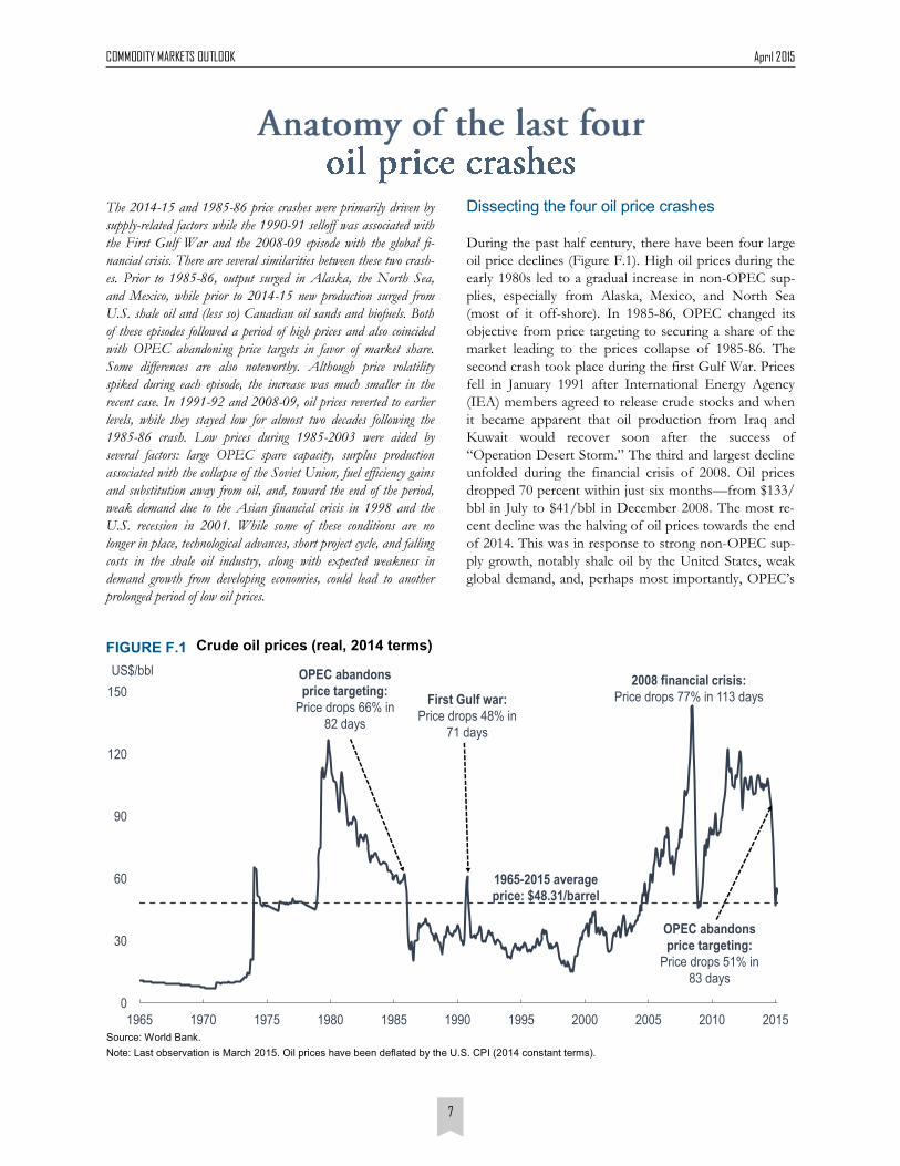
During the past half century, there have been four large

oil price declines (Figure F.1). High oil prices during the

early 1980s led to a gradual increase in non-OPEC sup-

plies, especially from Alaska, Mexico, and North Sea

(most of it off-shore). In 1985-86, OPEC changed its

objective from price targeting to securing a share of the

market leading to the prices collapse of 1985-86. The

second crash took place during the first Gulf War. Prices

fell in January 1991 after International Energy Agency

(IEA) members agreed to release crude stocks and when

it became apparent that oil production from Iraq and

Kuwait would recover soon after the success of

“Operation Desert Storm.” The third and largest decline

unfolded during the financial crisis of 2008. Oil prices

dropped 70 percent within just six months—from $133/

bbl in July to $41/bbl in December 2008. The most re-

cent decline was the halving of oil prices towards the end

of 2014. This was in response to strong non-OPEC sup-

ply growth, notably shale oil by the United States, weak

global demand, and, perhaps most importantly, OPEC’s

The 2014-15 and 1985-86 price crashes were primarily driven by

supply-related factors while the 1990-91 selloff was associated with

the First Gulf War and the 2008-09 episode with the global fi-

nancial crisis. There are several similarities between these two crash-

es. Prior to 1985-86, output surged in Alaska, the North Sea,

and Mexico, while prior to 2014-15 new production surged from

U.S. shale oil and (less so) Canadian oil sands and biofuels. Both

of these episodes followed a period of high prices and also coincided

with OPEC abandoning price targets in favor of market share.

Some differences are also noteworthy. Although price volatility

spiked during each episode, the increase was much smaller in the

recent case. In 1991-92 and 2008-09, oil prices reverted to earlier

levels, while they stayed low for almost two decades following the

1985-86 crash. Low prices during 1985-2003 were aided by

several factors: large OPEC spare capacity, surplus production

associated with the collapse of the Soviet Union, fuel efficiency gains

and substitution away from oil, and, toward the end of the period,

weak demand due to the Asian financial crisis in 1998 and the

U.S. recession in 2001. While some of these conditions are no

longer in place, technological advances, short project cycle, and falling

costs in the shale oil industry, along with expected weakness in

demand growth from developing economies, could lead to another

prolonged period of low oil prices.

FIGURE F.1

Source: World Bank.

Note: Last observation is March 2015. Oil prices have been deflated by the U.S. CPI (2014 constant terms).

Crude oil prices (real, 2014 terms)

0

30

60

90

120

150

1965 1970 1975 1980 1985 1990 1995 2000 2005 2010 2015

US$/bbl OPEC abandons

price targeting:

Price drops 66% in

82 days

First Gulf war:

Price drops 48% in

71 days

2008 financial crisis:

Price drops 77% in 113 days

OPEC abandons

price targeting:

Price drops 51% in

83 days

1965-2015 average

price: $48.31/barrel

8

COMMODITY MARKETS OUTLOOK April 2015

By 1985 Saudi Arabia had seen its oil production drop to

2.3 mb/d from 10 mb/d a few years earlier. Clearly if

Saudi Arabia had maintained its role as the swing pro-

ducer, it may have been driven out of the market. To

regain market share, it raised production, abandoned

official pricing, and adopted a spot pricing mechanism.

The 1990-91 crash The August 1990 Iraq invasion of Kuwait was preceded

by a lengthy period of low oil prices. Brent oil averaged

less than $17/bbl over the previous five years. Iraq’s

invasion of Kuwait and the subsequent Iraq war re-

moved more than 4 mb/d of combined Iraq/Kuwait

crude from the market. Other OPEC members, howev-

er, had large untapped capacity to fulfill this shortfall

that could be traced back to the early 1980s, when

OPEC had chosen to reduce production to defend high

prices. While other OPEC members were able to make

up the shortfall, it took some time to ramp up output.

Brent prices briefly eclipsed $40/bbl in September 1991

before slowly retreating to $28/bbl in December as addi-

tional supplies reached the market.

The ensuing price crash in mid-January 1991 was sharp

and sudden. Prior to the war the IEA agreed to release

changing objective from price targeting to market share

(as was the case in 1985-86).

The 1985-86 crash The collapse of oil prices in 1986 was preceded by sever-

al years of high (but declining) oil prices precipitated by

the Iranian Revolution. OPEC’s practice was to set offi-

cial prices for its various types of crude oil, with light oil

from Saudi Arabia used as the benchmark—it was set at

$34/bbl in 1981. High prices and a recession in the early

1980s led to a large decline in oil consumption, mainly in

advanced economies. High prices also encouraged fuel

conservation, substitution away from oil, especially in

electricity generation (some by nuclear power), and effi-

ciency gains—particularly higher minimum fuel efficien-

cy standards for automobiles. They also sparked non-

OPEC production, notably in Alaska, Mexico, and the

North Sea. Weak demand and rising non-OPEC output

led to a near halving of OPEC production, which was

mostly absorbed by Saudi Arabia. Saudi light prices de-

clined to $28/bbl in 1985, owing to sluggish global eco-

nomic activity and difficulties with the pricing system as

several member countries discounted official prices to

increase exports.

Summary statistics, the markets environment, and OPEC’s policies TABLE F.1

Notes: Comovement is defined as the proportion of prices that move in the same direction in a particular month, averaged over the 12-month period

before the end of the crash. It is bounded between zero and 100, zero implying that half of the price movements are up and half down and 100 imply-

ing that all prices move in the same direction, either up or down. Coefficient of variation is the standard deviation of prices (levels) divided by the

mean. Definitions of correlation between oil prices with equities and exchange rates and volatility of oil prices can be found in the box.

1985-86 1990-91 2008-09 2014-15

Key Statistics

Dates Nov 1985 to Mar 1986 Nov 1990 to Feb 1991 Jul 2008 to Feb 2009 Oct 2014 to Jan 2015

Duration (days) 82 71 113 83

Price drop (percent) 66 48 77 51

Volatility (percent) 4.69 5.18 4.62 2.58

Coefficient of variation 0.32 0.16 0.44 0.22

Comovement (percent) 27 19 48 25

Correlation with equities 0.01 0.03 0.12 0.06

Correlation with ex. rates 0.07 0.02 0.18 0.06

Market and Policy Environment

Fundamental drivers Increasing non-OPEC oil supplies, especially from Alaska, Mexico and the North Sea

Operation “Desert Storm” and IEA emergency stock draw calmed oil markets

Sell off of assets (including commodities) due to the 2008 financial crisis

Increasing non-OPEC oil supplies, especially shale oil from the U.S.

OPEC’s policy objective Protect market share rather than target prices

Keep oil market well-supplied

Target a price range Protect market share rather than target prices

OPEC’s action Raise production Raise production Cut production Raise production

Pre-crash oil prices Gradual decline of official OPEC prices

Sharp increase Large increase prior to the crash

Relatively stable prices above $100/bbl

Post-crash oil prices Remained low for almost two decades

Returned to pre-spike levels

Reached pre-crash levels within two years

They are projected to remain lower

9

COMMODITY MARKETS OUTLOOK April 2015

2.5 mb/d of emergency stocks in the event of war. This,

and the apparent early success of “Operation Desert

Storm,” prompted an immediate collapse in prices to

under $20/bbl. Thus, the 1991-92 crash was a reversion

of prices to their pre-spike levels following an external

shock, rather than following a prolonged period of high

prices, as in the other three cases.

The 2008-09 crash The largest post-WWII oil price decline came in response

to the 2008 financial crisis. During the second half of

2008, oil prices declined more than 70 percent. The price

collapse, which reflected uncertainly and a drastic reduc-

tion in demand, was not unique to oil. Most equity mar-

kets experienced similar declines, as did other commodity

prices, including other energy (such as coal), metals, food

commodities, and agricultural raw materials (such as nat-

ural rubber). The 2008 oil price crash was also accompa-

nied by a spike in volatility as well as closer comovement

across most commodity prices.

In the run-up to the 2008 financial crisis, OPEC had

reverted to restricting oil supplies in the early 2000s by

briefly targeting a price range of $22-28/bbl. However,

when prices exceeded that range in 2004, OPEC gradual-

ly raised its “preferred target” to $100-110/bbl. As the

financial crisis unfolded prices dropped to a low of less

than $40/bbl. Within the next two years prices surged

back to the $100 mark, helped by stronger demand as the

global economy rebounded and supported by OPEC’s

decision to take 4 mb/d off the market.

The 2014-15 crash The most recent crash took place against a backdrop of

high oil prices, weak demand, and strong oil supply

growth, especially from unconventional sources in the

United States (Arezki and Blanchard 2014; Baffes et al.

2015). During 2011-14, the United States alone added 4

mb/d to global oil supplies. Combined with two other

unconventional sources—Canadian oil sands and biofu-

els—more than 6 mb/d was added to the global oil mar-

ket. On the geopolitical front, some conditions eased.

Despite ongoing internal conflict, Libya added 0.5 mb/d

of production in the third quarter of 2014. Iraq’s oil out-

put turned out to be remarkably stable, at 3.3 mb/d dur-

ing 2014, the highest average since 1979. Even sanctions

imposed on Russia and ensuing countersanctions have

had little impact on European natural gas markets.

On the policy front, on November 27, 2014, OPEC an-

nounced that it would focus on preserving its market

share instead of maintaining a $100-110/bbl price range.

This shift in policy suggests that OPEC will no longer act

as the swing oil producer. Instead, the marginal cost pro-

ducers of unconventional oil are increasingly playing this

role (Kaletsky 2015). The steep price decline also coincid-

ed with a sharp appreciation of the U.S. dollar, which

trends to be negatively associated with U.S. dollar prices

of commodities, including oil (Frankel 2014; Zhang et al

2008; Akram 2009).

Contrasting the oil price crashes

There are multiple similarities and differences among the

four oil price crashes (Table F1). Most striking are the simi-

larities between the first and last crash. Both occurred after

a period of high prices, and rising non-OPEC oil supplies:

from Alaska, North Sea, and Mexico in 1985-86 and from

U.S. shale, Canadian oil sands, and biofuels in 2014-15. In

both crashes OPEC changed its policy objective, from

price targeting to market share. There is a similarity be-

tween the 1990-91 and 2008-09 crashes as well, in that

Source: World Bank.

Note: Details on the volatility measures are discussed in the box.

Volatility of oil price during the four crashes

FIGURE F.3

0

1

2

3

4

5

6

1985-86 1990-91 2008-09 2014-15

Standard deviation of returns Interquartile range

GARCH (full sample) GARCH (250-day window)

Correlation between oil price and financial variables

FIGURE F.2

Source: World Bank Note: Correlation refers to the R-square of the respective regression.

0.00

0.05

0.10

0.15

0.20

0.25

0.30

1985-86 1990-91 2008-09 2014-15

Exchange rate

Equity (S&P 500)

Exchange rate and equity

10

COMMODITY MARKETS OUTLOOK April 2015

both were precipitated by global events: the First Gulf War

(the former) and the 2008 financial crisis (the latter).

There are also key differences, with the 2008-09 crash ex-

hibiting some unique characteristics. Prices during that

crash were highly correlated with equity and exchange rate

movements (Figure F.2). Similarly, comovement across

most commodity prices was high during 2008—twice as

high compared to the historical average (and other crash-

es). However, although volatility spiked during all four

episodes, the increase was much smaller (and began much

later) during the last crash, a result consistent across several

measures of volatility (Figure F.3).

Current conditions compared with 1985-86

Following the 1985-86 collapse, oil prices remained rela-

tively low for almost two decades. Brent prices averaged

$20/bbl between November 1985 and December 2003,

beginning and ending the period at about $30/bbl. Prices

were kept in check for several reasons, both supply and

demand related, and OPEC policy.

On the supply side, OPEC’s spare capacity stood at a mas-

sive 12 mb/d in 1985 (Figure F.4). A surplus also devel-

oped in the former Soviet Union (FSU) during the transi-

tion of the 1990s. Although FSU oil production fell by 5.5

mb/d initially, most was brought back on line (Figure F.5).

These supply cushions kept oil prices low for several years.

On the demand side, the efficiency gains in the automobile

sector in the 1970s and early 1980s came to a halt as lower

prices led consumer preference to less efficient vehicles—

U.S. efficiency standards for passenger cars remained at

27.5 miles per gallon during 1985-2010. Substitution away

from oil slowed as well. Oil demand grew relatively strong-

ly in industrial countries over the next 20 years (1.5 percent

per annum or 6.8 mb/d during 1985-2005). However,

growth was larger in non-OECD countries outside the

FSU, rising by 4.2 percent per annum, or 16.8 mb/d.

Some of the conditions behind the low oil prices of 1985-

2003 are no longer in place. First, OPEC’s spare capacity

is significantly lower now than it was in 1985. According

to the IEA, OPEC spare capacity today is 2.5 mb/d

(excluding Iraq, Iran, Libya and Nigeria). Oil demand

conditions in the OECD have changed dramatically.

High prices and new efficiency standards have led to

decline in OECD consumption since 2005 of nearly 5

mb/d. Most forecasts show little or no growth in OECD

consumption going forward, and some show declines due

to anticipated increases in fuel efficiency and environ-

mental constraints. Given that developing and emerging

economies consume much less oil in per capita terms,

potential still remains for significant growth in con-

sumption where most the gains are expected to occur.

There are some factors that could lead to a prolonged

period of low oil prices. On the supply side, U.S. shale

oil production provided much of the growth during the

past five years. Although shale oil costs vary widely

(some well below $50/bbl and others above $70/bbl),

the industry’s production costs are falling due to greater

operational knowledge, improved technologies, and

lower input prices. Thus, shale oil production may be

sustained at higher-than-expected levels. On the de-

mand side, if the global prospects in emerging and de-

veloping economies remain muted, oil consumption

growth may suffer. Lastly, technological breakthroughs,

either through improvement in battery technology or

further use of natural gas in transportation, are less like-

ly to materialize at current oil prices (say, $50-60/bbl

range) than they would be at, say, the $100-110/bbl

price range.

Former Soviet Union oil produc-tion and consumption

FIGURE F.5

Source: BP Statistical Review (June 2014 update).

0

3

6

9

12

15

1985 1990 1995 2000 2005 2010

mb/d

Russian Federation production

Former Soviet Union consumption

Former Soviet Union production

15

20

25

30

35

1980 1985 1990 1995 2000 2005

mb/d

Capacity

Production

OPEC production and capacity FIGURE F.4

Source: KBC Energy Economics.

11

COMMODITY MARKETS OUTLOOK April 2015

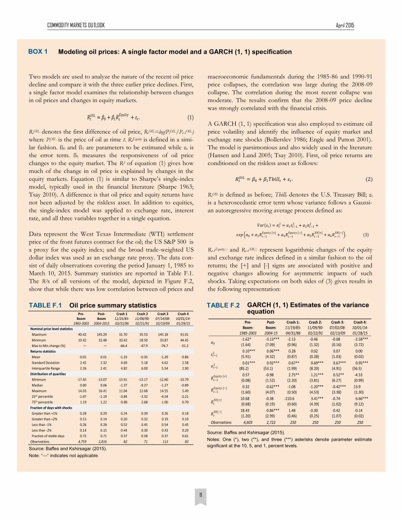
Modeling oil prices: A single factor model and a GARCH (1, 1) specification BOX 1

Two models are used to analyze the nature of the recent oil price

decline and compare it with the three earlier price declines. First,

a single factor model examines the relationship between changes

in oil prices and changes in equity markets.

RtOIL denotes the first difference of oil price, RtOIL=log(PtOIL/Pt-1OIL)

where PtOIL is the price of oil at time t. RtEquity is defined in a simi-

lar fashion. ß0 and ß1 are parameters to be estimated while εt is

the error term. ß1 measures the responsiveness of oil price

changes to the equity market. The R2 of equation (1) gives how

much of the change in oil price is explained by changes in the

equity markets. Equation (1) is similar to Sharpe’s single-index

model, typically used in the financial literature (Sharpe 1963;

Tsay 2010). A difference is that oil price and equity returns have

not been adjusted by the riskless asset. In addition to equities,

the single-index model was applied to exchange rate, interest

rate, and all three variables together in a single equation.

Data represent the West Texas Intermediate (WTI) settlement

price of the front futures contract for the oil; the US S&P 500 is

a proxy for the equity index; and the broad trade-weighted US

dollar index was used as an exchange rate proxy. The data con-

sist of daily observations covering the period January 1, 1985 to

March 10, 2015. Summary statistics are reported in Table F.1.

The R2s of all versions of the model, depicted in Figure F.2,

show that while there was low correlation between oil prices and

macroeconomic fundamentals during the 1985-86 and 1990-91

price collapses, the correlation was large during the 2008-09

collapse. The correlation during the most recent collapse was

moderate. The results confirm that the 2008-09 price decline

was strongly correlated with the financial crisis.

A GARCH (1, 1) specification was also employed to estimate oil

price volatility and identify the influence of equity market and

exchange rate shocks (Bollerslev 1986; Engle and Patton 2001).

The model is parsimonious and also widely used in the literature

(Hansen and Lund 2005; Tsay 2010). First, oil price returns are

conditioned on the riskless asset as follows:

RtOIL is defined as before; Tbillt denotes the U.S. Treasury Bill; εt

is a heteroscedastic error term whose variance follows a Gaussi-

an autoregressive moving average process defined as:

Rt-1Equity[.] and Rt-1XR[.] represent logarithmic changes of the equity

and exchange rate indices defined in a similar fashion to the oil

returns; the [+] and [-] signs are associated with positive and

negative changes allowing for asymmetric impacts of such

shocks. Taking expectations on both sides of (3) gives results in

the following representation:

𝑉𝑎𝑟 𝜀𝑡 = 𝜎𝑡2 = 𝛼1𝜀𝑡−1

2 + 𝛼2𝜎𝑡−12 +

𝑒𝑥𝑝 𝛼0 + 𝛼3𝑅𝑡−1𝐸𝑞𝑢𝑖𝑡𝑦 [+]

+ 𝛼4𝑅𝑡−1𝐸𝑞𝑢𝑖𝑡𝑦 [−]

+ 𝛼5𝑅𝑡−1𝑋𝑅[+]

+ 𝛼6𝑅𝑡−1𝑋𝑅[−]

. (3)

Oil price summary statistics TABLE F.1

Source: Baffes and Kshirsagar (2015).

Note: “—“ indicates not applicable.

Pre- Boom

1983-2003

Post-Boom

2004-2015

Crash 1 11/25/85-03/31/86

Crash 2 11/08/90-02/21/91

Crash 3 07/14/08-02/19/09

Crash 4 10/01/14-01/29/15

Nominal price level statistics

Maximum 40.42 145.29 31.70 35.53 145.18 91.01

Minimum 10.42 32.48 10.42 18.50 33.87 44.45

Max to Min change (%) — — -66.4 -47.9 -76.7 -51.2

Returns statistics

Mean 0.01 0.01 -1.33 -0.35 -1.29 -0.86

Standard Deviation 2.42 2.32 4.69 5.18 4.62 2.58

Interquartile Range 2.26 2.41 4.82 6.00 5.54 2.90

Distribution of quartiles

Minimum -17.45 -13.07 -13.91 -13.17 -12.60 -10.79

Median 0.00 0.06 -1.37 -0.27 -1.27 -0.89

Maximum 14.03 16.41 11.04 12.68 14.55 5.49

25th percentile -1.07 -1.19 -3.84 -3.32 -4.54 -2.21

75th percentile 1.19 1.22 0.98 2.68 1.00 0.70

Fraction of days with shocks

Greater than +1% 0.28 0.29 0.24 0.39 0.26 0.18

Greater than +2% 0.15 0.14 0.20 0.32 0.19 0.10

Less than -1% 0.26 0.28 0.52 0.45 0.54 0.45

Less than -2% 0.14 0.15 0.44 0.30 0.43 0.29

Fraction of stable days 0.72 0.71 0.37 0.38 0.37 0.61

Observations 4,759 2,816 82 71 113 83

GARCH (1, 1) Estimates of the variance equation

TABLE F.2

Source: Baffes and Kshirsagar (2015).

Notes: One (*), two (**), and three (***) asterisks denote parameter estimate

significant at the 10, 5, and 1, percent levels.

Pre- Boom:

1985-2003

Post-Boom:

2004-15

Crash 1: 11/19/85-04/31/86

Crash 2: 11/09/90-02/22/91

Crash 3: 07/02/08-02/13/09

Crash 4: 10/01/14-01/28/15

𝛼0 -1.62* (1.64)

-3.13*** (7.09)

-2.13 (0.96)

-0.46 (1.32)

-0.08 (0.16)

-2.58*** (3.72)

𝜀𝑡−12

0.10*** (5.91)

0.06*** (4.32)

0.28 (0.87)

0.02 (0.28)

0.07 (1.03)

0.00 (0.02)

𝜎𝑡−12

0.01*** (85.2)

0.92*** (53.1)

0.67** (1.99)

0.69*** (8.20)

0.67*** (4.91)

0.95*** (56.5)

𝑅𝑡−1𝐸𝑞𝑢𝑖𝑡𝑦 [+]

0.57

(0.08) -0.98 (1.52)

2.75** (2.20)

1.21*** (3.81)

0.52** (6.27)

-4.53 (0.99)

𝑅𝑡−1𝐸𝑞𝑢𝑖𝑡𝑦 [−]

0.32

(1.60) -0.62*** (4.07)

-1.08 (0.50)

-1.20*** (4.53)

-0.42*** (3.38)

13.9 (1.30)

𝑅𝑡𝑋𝑅 [+]

10.68 (0.68)

-0.38 (0.19)

-210.6 (0.60)

3.41*** (4.39)

-0.74 (1.02)

6.66*** (9.12)

𝑅𝑡𝑋𝑅 [−]

18.43 (1.20)

-0.86*** (2.99)

1.48 (0.46)

-0.30 (0.25)

-0.42 (1.07)

-0.14 (0.02)

Observations 4,603 2,722 250 250 250 250

𝑅𝑡𝑂𝐼𝐿 = 𝛽0 + 𝛽1𝑅𝑡

𝐸𝑞𝑢𝑖𝑡𝑦+ 𝜀𝑡 . (1)

𝑅𝑡𝑂𝐼𝐿 = 𝛽0 + 𝛽1𝑇𝑏𝑖𝑙𝑙𝑡 + 𝜀𝑡 . (2)

12

COMMODITY MARKETS OUTLOOK April 2015

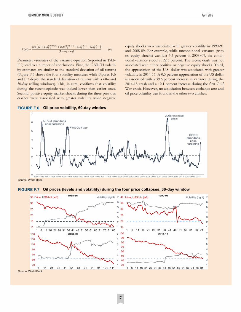
Parameter estimates of the variance equation (reported in Table

F.2) lead to a number of conclusions. First, the GARCH volatil-

ity estimates are similar to the standard deviation of oil returns

(Figure F.3 shows the four volatility measures while Figures F.6

and F.7 depict the standard deviation of returns with a 60– and

30-day rolling windows). This, in turn, confirms that volatility

during the recent episode was indeed lower than earlier ones.

Second, positive equity market shocks during the three previous

crashes were associated with greater volatility while negative

equity shocks were associated with greater volatility in 1990-91

and 2008-09. For example, while unconditional variance (with

no equity shocks) was just 3.5 percent in 2008/09, the condi-

tional variance stood at 22.3 percent. The recent crash was not

associated with either positive or negative equity shocks. Third,

the appreciation of the U.S. dollar was associated with greater

volatility in 2014-15. A 0.5 percent appreciation of the US dollar

is associated with a 39.6 percent increase in variance during the

2014-15 crash and a 12.1 percent increase during the first Gulf

War crash. However, no association between exchange arte and

oil price volatility was found in the other two crashes.

𝐸 𝜎2 =𝑒𝑥𝑝 𝛼0 + 𝛼3𝑅𝑡−1

𝐸𝑞𝑢𝑖𝑡𝑦 [+]+ 𝛼4𝑅𝑡−1

𝐸𝑞𝑢𝑖𝑡𝑦 [−]+ 𝛼5𝑅𝑡−1

𝑋𝑅[+]+ 𝛼6𝑅𝑡−1

𝑋𝑅[−]

1 − 𝛼1 − 𝛼2 . (4)

Oil prices (levels and volatility) during the four price collapses, 30-day window FIGURE F.7

Source: World Bank

1

2

3

4

5

6

7

10

15

20

25

30

35

1 6 11 16 21 26 31 36 41 46 51 56 61 66 71 76 81 86

1

2

3

4

5

6

7

15

20

25

30

35

40

1 6 11 16 21 26 31 36 41 46 51 56 61 66 71

Price, US$/bbl (left) Volatility (right)

1

2

3

4

5

6

7

30

50

70

90

110

130

150

1 11 21 31 41 51 61 71 81 91 101 111

1

2

3

4

5

6

7

30

40

50

60

70

80

90

100

1 6 11 16 21 26 31 36 41 46 51 56 61 66 71 76 81

1985-86 1990-91

2008-09 2014-15

Price, US$/bbl (left) Volatility (right)

FIGURE F.6 Oil price volatility, 60-day window

Source: World Bank

0

1

2

3

4

5

6

7

1985 1986 1987 1988 1989 1990 1991 1992 1993 1994 1995 1996 1997 1998 1999 2000 2001 2002 2003 2004 2005 2006 2007 2008 2009 2010 2011 2012 2013 2014

OPEC abandons

price targeting

First Gulf war

2008 financial

crisis

OPEC

abandons

price

targeting

13

COMMODITY MARKETS OUTLOOK April 2015

References

Akram, Q. F. (2009). “Commodity prices, interest rate,

and the dollar.” Energy Economics, 31, 838-851.

Arezki, R. and O. Blanchard (2014). “Seven questions

about the recent oil price slump.” IMF Blog, Decem-ber 22. International Monetary Fund. Washington, D.C.

Baffes, J., M.A. Kose, F. Ohnsorge, and M. Stocker

(2015). The great plunge in oil prices: Causes, consequences, and policy responses, Policy Research Note 15/01. The World Bank. Washington, D.C.

Baffes, J. and V. Kshirsagar (2015). “Sources of volatility

during four oil price crashes.” Mimeo, Development Prospects Group, The World Bank. Washington, D.C.

Bollerslev, T. (1986). “Generalized autoregressive condi-

tional heteroskedasticity.” Journal of Econometrics, 31, 307-327.

Engle, R.F. and A.J. Patton (2001). “What good is a vola-

tility model?” Quantitative Finance, 1, 237-245.

Frankel, J. (2014). “Why Are Commodity Prices Falling?”

Project Syndicate, December 15.

Hansen, P.R. and A. Lunde (2005). “A forecast compari-

son of volatility models: Does anything beat a GARCH (1, 1)?” Journal of Applied Econometric, 20, 873-889.

Kaletsky, A. (2015). “A new ceiling for oil prices.” Pro-

ject Syndicate, January 14.

Sharpe, W.F. (1964). “Capital asset prices: A theory of

market equilibrium under conditions of risk.” Journal

of Finance, 19, 425-442.

Tsay, R. (2010). Analysis of financial time series. John Wiley

& Sons.

Zhang, Y. Y. Fan, H. Tsai, and Y. Wei (2008). “Spillover

Effect of U.S. Dollar Exchange Rate on Oil Prices.”

Journal of Policy Modelling, 30, pp. 973-991.