Oct/Nov/Dec Vol 27 No 4

The Stata News

Executive Editor ..............Karen Strope

Production Supervisor .....Annette Fett

Coming soon from Stata Press

Introduction to Time Series Using Stata

Author: Sean Becketti

Publisher: Stata Press

Copyright: 2013

ISBN-13: 978-1-59718-132-7 Price: $59.00

Introduction to Time Series Using Stata, by Sean Becketti, provides a practical guide to working with time-series data using Stata and will appeal to a broad range of users. The many examples, concise explanations that focus on intuition, and useful tips based on the author’s decades of experience using time-series methods make the book insightful not just for academic users but also for practitioners in industry and government.

The book is appropriate both for new Stata users and for experienced users who are new to time-series analysis.

Chapter 1 provides a mild yet fast-paced introduction to Stata, highlighting all the features a user needs to know to get started using Stata for time-series analysis. Chapter 2 is a quick refresher on regression and hypothesis testing, and it defines key concepts such as white noise, autocorrelation, and lag operators.

Chapter 3 begins the discussion of time series, using moving-average and Holt–Winters techniques to smooth and forecast the data. Becketti also introduces the concepts of trends, cyclicality, and seasonality and shows how they can be extracted from a series. Chapter 4 focuses on using these methods for forecasting and illustrates how the assumptions regarding trends and cycles underlying the various moving-average and Holt–Winters techniques affect the forecasts produced. Although these techniques are sometimes neglected in other time-series books, they are easy to implement, can be applied to many series quickly, often produce forecasts just as good as more complicated techniques, and as Becketti emphasizes, have the distinct advantage of being easily explained to colleagues and policy makers without backgrounds in statistics.

Chapters 5 through 8 encompass single-equation time-series models. Chapter 5 focuses on

regression analysis in the presence of autocorrelated disturbances and details various approaches that can be used when all the regressors are strictly exogenous but the errors are autocorrelated, when the set of regressors includes a lagged dependent variable and independent errors, and when the set of regressors includes a lagged dependent variable and autocorrelated errors. Chapter 6 describes the ARIMA model and Box–Jenkins methodology, and chapter 7 applies those techniques to develop an ARIMA-based model of U.S. GDP. Chapter 7 in particular

In the spotlight: marginsplot .........2

In the spotlight: Fractals ...............4

2013 Stata Conference ..................5

Visit us at ASSA 2013 ....................5

New from the Stata Bookstore .....5

Public training course ...................7

NetCourse schedule ......................7

Stata is now on YouTube ...............8

Continued on p.6

In the spotlight: marginsplot

If you’ve ever felt stymied when trying to explain polynomial terms, odds ratios, interactions, or (gasp!) coefficients from a probit model, you will be interested in exploring the margins and marginsplot commands in Stata. Together, they enable you to visualize how inputs affect outputs in statistical models.

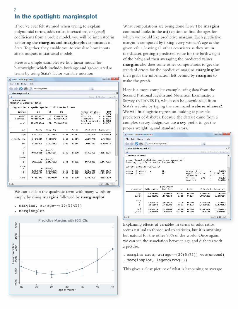
Here is a simple example: we fit a linear model for birthweight, which includes both age and age-squared as terms by using Stata’s factor-variable notation:

We can explain the quadratic term with many words or simply by using margins followed by marginsplot.

. margins, at(age==(15(5)45))

. marginsplot

What computations are being done here? The margins command looks in the at() option to find the ages for which we would like predictive margins. Each predictive margin is computed by fixing every woman’s age at the given value, leaving all other covariates as they are in the dataset, getting a predicted value for the birthweight of the baby, and then averaging the predicted values. margins also does some other computations to get the standard errors for the predictive margins. marginsplot then grabs the information left behind by margins to make the graph.

Here is a more complex example using data from the Second National Health and Nutrition Examination Survey (NHANES II), which can be downloaded from Stata’s website by typing the command webuse nhanes2. We will fit a logistic regression looking at possible predictors of diabetes. Because the dataset came from a complex survey design, we use a svy prefix to get the proper weighting and standard errors.

Explaining effects of variables in terms of odds ratios seems natural to those used to statistics, but it is anything but natural for the other 90% of the world. Once again, we can see the association between age and diabetes with a picture.

. margins race, at(age==(20(5)75)) vce(uncond)

. marginsplot, legend(row(1))

This gives a clear picture of what is happening to average

2

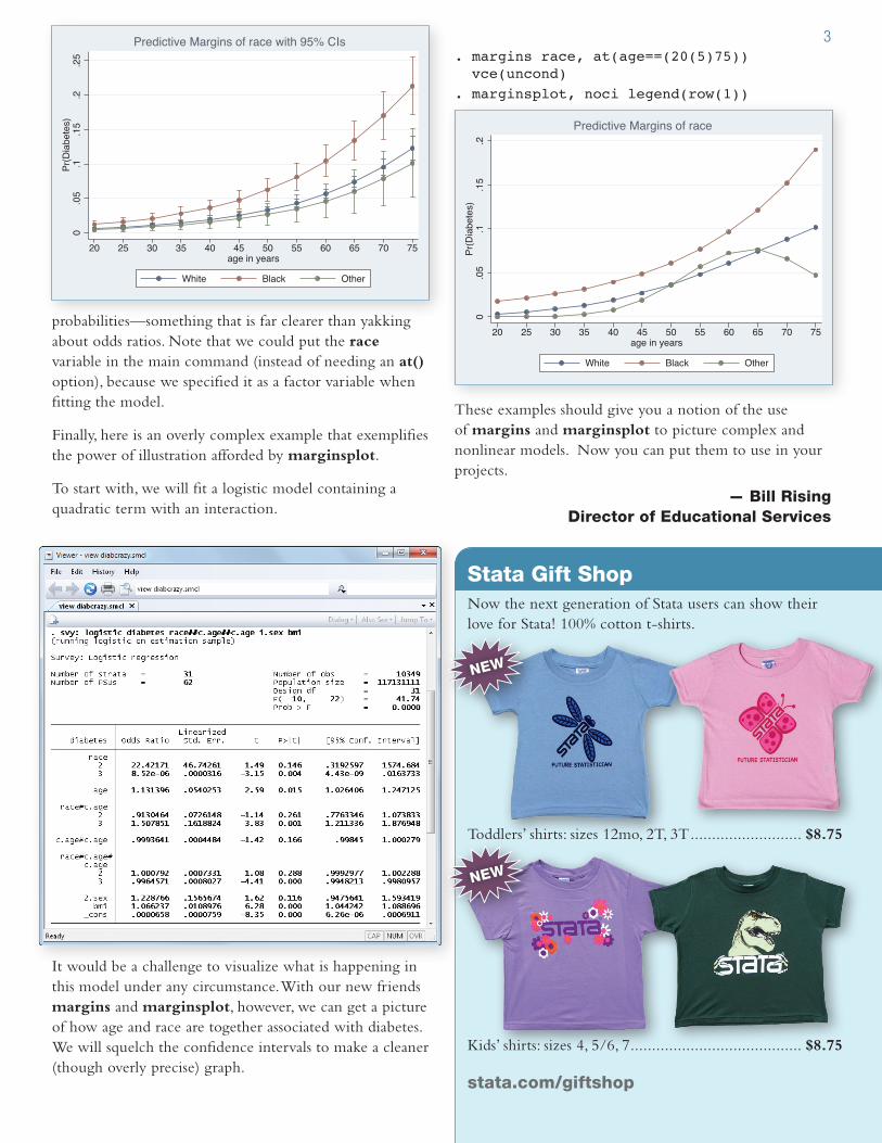
probabilities—something that is far clearer than yakking about odds ratios. Note that we could put the race variable in the main command (instead of needing an at() option), because we specified it as a factor variable when fitting the model.

Finally, here is an overly complex example that exemplifies the power of illustration afforded by marginsplot.

To start with, we will fit a logistic model containing a quadratic term with an interaction.

It would be a challenge to visualize what is happening in this model under any circumstance. With our new friends margins and marginsplot, however, we can get a picture of how age and race are together associated with diabetes. We will squelch the confidence intervals to make a cleaner (though overly precise) graph.

. margins race, at(age==(20(5)75)) vce(uncond). marginsplot, noci legend(row(1))

These examples should give you a notion of the use of margins and marginsplot to picture complex and nonlinear models. Now you can put them to use in your projects.

— Bill Rising Director of Educational Services

Stata Gift Shop

Toddlers’ shirts: sizes 12mo, 2T, 3T .......................... $8.75

Kids’ shirts: sizes 4, 5/6, 7 ........................................ $8.75

stata.com/giftshop

Now the next generation of Stata users can show their love for Stata! 100% cotton t-shirts.

NEW

NEW

3

In the spotlight: Fractals

The Mandelbrot set is perhaps the most well-known fractal set. It is defined by the simple recursion

Zn+1

= Zn2 + C

where Zn and C are complex numbers. Say we choose

a value for C and draw a circle of radius R centered at the origin of the (x, y) plane. For any point in the plane, we can then perform the recursion starting at the point Z

1 = x + yi and see how many iterations are required for

Zn to escape the circle. We can repeat this exercise for an

entire grid of points and use a contour plot to show the number of iterations required for each point in the grid.

Mata, coupled with Stata’s strong graphics and data management capabilities, is highly suited to dealing with mathematical objects such as fractals. It also lets us show off how easy it is to work with complex numbers in Mata.

We can easily code the recursion in Mata. This function takes a point Z in the complex plane along with a selected radius R and constant C and returns the number of iterations required to escape the circle. To avoid a potential infinite loop, this function also takes a maximum number of iterations to perform.

mata:real scalar escape(complex scalar Z, C, real scalar R, maxiter){ real scalar i for (i=0; i<maxiter; i++) { if (norm(Z) <= R) { Z = Z*Z+C } else return(i) } return(i)} end

Now we can compute the escape values for each point in a 200-by-200 grid, given C = -0.8 + 0.156i and R = 100.

mata:res = J(201*201, 3, .)cnt = 1C = -0.8+0.156ifor(i=0; i<=200; i++) { for(j=0; j<=200; j++) { Z = C(-2+i*4/200, -2+j*4/200) n = escape(Z, C, 100, 400) mandelbrot_set[cnt, .] = (i, j, n) cnt++ }}end

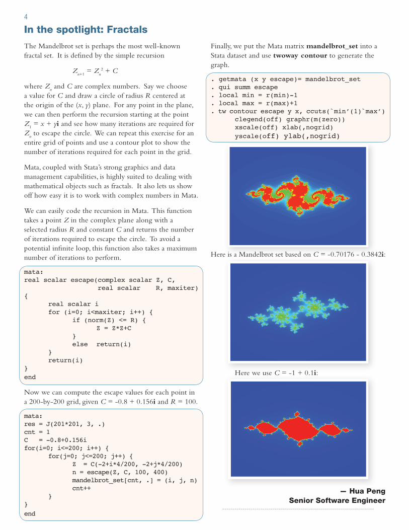
Finally, we put the Mata matrix mandelbrot_set into a Stata dataset and use twoway contour to generate the graph.

. getmata (x y escape)= mandelbrot_set

. qui summ escape

. local min = r(min)-1

. local max = r(max)+1

. tw contour escape y x, ccuts(`min’(1)`max’) clegend(off) graphr(m(zero)) xscale(off) xlab(,nogrid) yscale(off) ylab(,nogrid)

Here is a Mandelbrot set based on C = -0.70176 - 0.3842i:

Here we use C = -1 + 0.1i:

— Hua Peng Senior Software Engineer

4

New from the Stata Bookstore

Introductory Econometrics: A Modern Approach, Fifth Edition

Author: Jeffrey M. Wooldridge

Publisher: South-Western (Cengage Learning)

Copyright: 2013

ISBN-13: 978-1-111-53104-1

Pages: 881; hardcover

Price: $198.00

The fifth edition of Jeffrey Wooldridge’s textbook, Introductory Econometrics: A Modern Approach, lives up to its subtitle in its choice of topics and its treatment of standard material.

Wooldridge recognizes that modern econometrics involves much more than ordinary least squares (OLS) with a few extensions to handle the special cases commonly encountered in econometric data. In addition to chapters on OLS, he includes chapters on current techniques of estimation and inference for time-series data, panel data, limited dependent variables, and sample selection.

In his treatments of OLS and two-stage least squares, Wooldridge breaks new ground by concentrating on advanced statistical concepts instead of matrix algebra. A traditional approach to introductory econometrics would use advanced sections to explain matrix algebra and its applications in econometrics. In contrast, Wooldridge uses the advanced sections of his text to introduce recently developed statistical concepts and techniques. This approach leads to a text with greater breadth than is usual in books of this type. This book is equally useful for advanced undergraduate study, as the basis of a survey course at the graduate level, or as a conceptual supplement to advanced courses.

The fifth edition contains a new section that highlights the differences between a model and an estimator as well as expanded treatments of models for proportional dependent variables, of using proxy variables to model unobserved confounders, and of least absolute-deviations estimators. The result is that an excellent introductory book has been made even better.

You can find the table of contents and online ordering information at stata.com/bookstore/introductory-econometrics.

Visit us at ASSA 2013

San Diego, California

January 4–6, 2013

The Allied Social Science Association (ASSA) will have its annual meeting in San Diego, CA, from January 4–6. For more information, visit aeaweb.org/Annual_Meeting.

Stata representatives, including David M. Drukker, Director of Econometrics, and Brian P. Poi, Senior Economist, will be available to answer your questions about Stata and demonstrate the new features in Stata 12. Stop by booth #401 to visit with the people who develop and support the software.

NEW ORLEANSJULY 18-19, 2013

Save the date: Stata Conference

Venue: Hyatt French Quarter New Orleans800 Iberville StreetNew Orleans, Louisiana 70112frenchquarter.hyatt.com

Chair: R. Carter Hill Louisiana State University

stata.com/new-orleans13

5

Cuadernos Metodológicos: Análisis de datos con Stata, Segunda Edición

Authors: Modesto Escobar Mercado, Enrique Fernández Macías, and Fabrizio Bernardi

Publisher: Centro de Investigaciones Sociologicas

Copyright: 2012

ISBN-13: 978-84-7476-588-5

Pages: 513; paperback

Price: $47.00

Análisis de datos con Stata, por Escobar, Fernández, y Bernardi, es un excelente recurso para usuarios de Stata con niveles de principiante o intermedio y que desean familiarizarse rápidamente con las facilidades que ofrece el software para el manejo de los datos y el análisis estadístico.

Los autores ilustran el uso de Stata para estadística descriptiva y análisis de regresión, usando ejemplos que están principalmente enfocados en investigaciones asociadas a las ciencias sociales, pero que son fáciles de seguir por usuarios en diferentes áreas de trabajo.

The book is in Spanish. You can find the table of contents and online ordering information at stata.com/bookstore/cuadernos-metodologicos.

will appeal to practitioners because it goes step by step through a real-world example: here is my series, now how do I fit an ARIMA model to it? Chapter 8 is a self-contained summary of ARCH/GARCH modeling.

In the final portion of the book, Becketti discusses multiple-equation models, particularly VARs and VECs. Chapter 9 focuses on VAR models and illustrates all key concepts, including model specification, Granger causality, impulse-response analyses, and forecasting, using a simple model of the U.S. economy;

structural VAR models are illustrated by imposing a Taylor rule on interest rates. Chapter 10 presents nonstationary time-series analysis. After describing nonstationarity and unit-root tests, Becketti masterfully navigates the reader through the often-confusing task of specifying a VEC model, using an example based on construction wages in Washington, DC, and surrounding states. Chapter 11 concludes.

Sean Becketti is a financial industry veteran with three decades of experience in academics, government, and private industry. He was a

developer of Stata in its infancy, and he was Editor of the Stata Technical Bulletin, the precursor to the Stata Journal, between 1993 and 1996. He has been a regular Stata user since its inception, and he wrote many of the first time-series commands in Stata.

Introduction to Time Series Using Stata, by Sean Becketti, is a first-rate, example-based guide to time-series analysis and forecasting using Stata. It can serve as both a reference for practitioners and a supplemental textbook for students in applied statistics courses.

Preorder today!stata-press.com/book/introduction-to-time-series-using-stata

Begins shipping December 2012.

Coming soon from Stata Press

Continued from p.1

Introduction to Time Series Using Stata

6

Public training

Using Stata Effectively: Data Management, Analysis, and Graphics FundamentalsBecome intimately familiar with all three components of Stata: data management, analysis, and graphics. This two-day course is aimed at new Stata users and those who wish to learn techniques for efficient day-to-day use of Stata. Upon completion of the course, you will be able to use Stata efficiently for basic analyses and graphics. You will be able to do this in a reproducible manner, making collaborative changes and follow-up analyses much simpler. Finally, you will be able to make your datasets self-explanatory to your co-workers and yourself when using them in the future.

Course outline

• Stata basics › Keeping organized › Knowing how Stata treats data › Using dialog boxes efficiently › Using the Command window › Saving time and effort while working

• Data management › Reading in datasets of various standard formats › Labeling variables and setting up encoded variables › Generating new variables in an efficient fashion › Combining datasets by adding observations and by

adding variables › Reshaping datasets for repeated measurements

• Workflow › Using menus and the Command window › Setting up Stata to one’s liking › Keeping complete records › Creating reproducible analyses › Finding, installing, and removing user-written

extensions to Stata › Customizing Stata

• Analysis › Using basic statistical commands › Reusing results of Stata commands › Using common postestimation commands › Working with interactions and factor variables

• Graphics › Making common, simple graphs › Building up complex graphs › Using the Graph Editor

January 9–10 .................................... Washington, DC

February 5–6 .................................... Washington, DC

March 12–13 .................................. New York City, NY

Enrollment for this course is $950. We offer a 15% discount for group enrollments of three or more participants. Contact us at training@stata.com for details. For course details, or to enroll, visit stata.com/training/using-stata-effectively.

NetCourse® schedule

NetCourses are convenient, web-based courses for learning Stata. Enroll by visiting stata.com/netcourse.

NetCourse 101, Introduction to StataThis introductory course is designed to take smart, knowledgeable people and turn them into proficient interactive users of Stata. It covers techniques and tricks to make you a powerful Stata user.

Dates: January 18–March 1, 2013 Price: $95stata.com/netcourse/intro-nc101

NetCourse 151, Introduction to Stata ProgrammingThis course teaches what most statistical software users mean by programming, namely, the careful performance of reproducible analyses.

Dates: January 18–March 1, 2013 Price: $125stata.com/netcourse/programming-intro-nc151

NetCourseNow Would you prefer to choose the time and set the pace of a NetCourse? Want to have a personal instructor? NetCourseNow is for you: stata.com/netcourse/ncnow.

7

Contact us979-696-4600 979-696-4601 (fax)service@stata.com stata.comPlease include your Stata serial number with all correspondence.

Find a Stata distributor near you stata.com/worldwide

Copyright 2012 by StataCorp LP.

StataCorp4905 Lakeway DriveCollege Station, TX 77845-4512USA

Return service requested.

Serious software for serious researchers. Stata is a registered trademark of StataCorp LP. Serious software for serious researchers is a trademark of StataCorp LP.

facebook.com/StataCorp twitter.com/Stata blog.stata.com

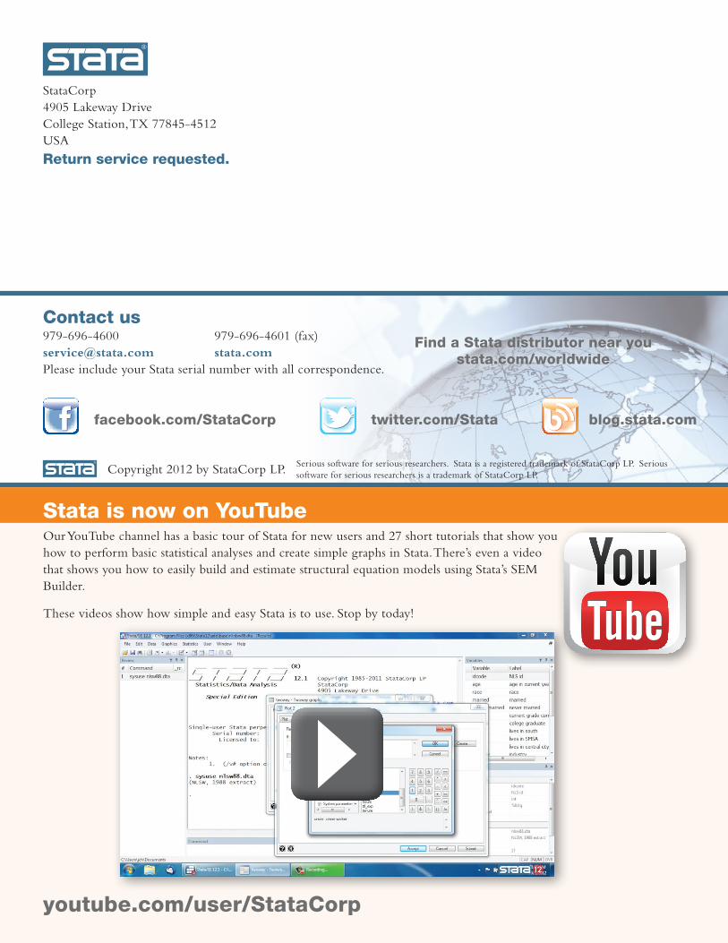
Stata is now on YouTubeOur YouTube channel has a basic tour of Stata for new users and 27 short tutorials that show you how to perform basic statistical analyses and create simple graphs in Stata. There’s even a video that shows you how to easily build and estimate structural equation models using Stata’s SEM Builder.

These videos show how simple and easy Stata is to use. Stop by today!

youtube.com/user/StataCorp