Turbulent mixing for a jet in crossflow and plans for turbulent combustion simulations
Turbulent Combustion Modeling
Combustion Summer School
Prof. Dr.-Ing. Heinz Pitsch
2018

Course Overview
2
• Turbulence
• Turbulent Premixed Combustion
• Turbulent Non-Premixed
Combustion
• Turbulent Combustion Modeling
• Applications
• Moment Methods for reactive scalars
• Simple Models in Fluent: EBU,EDM, FRCM,
EDM/FRCM
• Introduction in Statistical Methods: PDF,
CDF,…
• Transported PDF Model
• Modeling Turbulent Premixed Combustion
• BML-Model
• Level Set Approach/G-equation
• Modeling Turbulent Non-Premixed
Combustion
• Conserved Scalar Based Models for
Non-Premixed Turbulent Combustion
• Flamelet-Model
• Application: RIF, steady flamelet model
Part II: Turbulent Combustion

Moment Methods for Reactive Scalars
Balance Equation for Reactive Scalars
• The term „reactive scalar“
Mass fraction Yα of all components α = 1, … N
Temperature T
• Balance equation for
Di: mass diffusivity, thermal diffusivity
Si: mass/temperature source term
3

Balance Equation for Reactive Scalars
• Neglecting the molecular transport (assumption: Re↑)
• Gradient transport assumption for the turbulent transport
→ Averaged transport equation
→ Simplest possible approach: Express unclosed terms as a function of mean values
4
not closed

Moment Methods for Reactive Scalars: Error Estimation
• Assumption: heat release expressed by
B: includes frequency factor und heat of reaction
Tb: adiabatic flame temperature
E: activation energy
• Approach for modeling the chemical source term
• Proven method Decomposition into mean and fluctuation
5
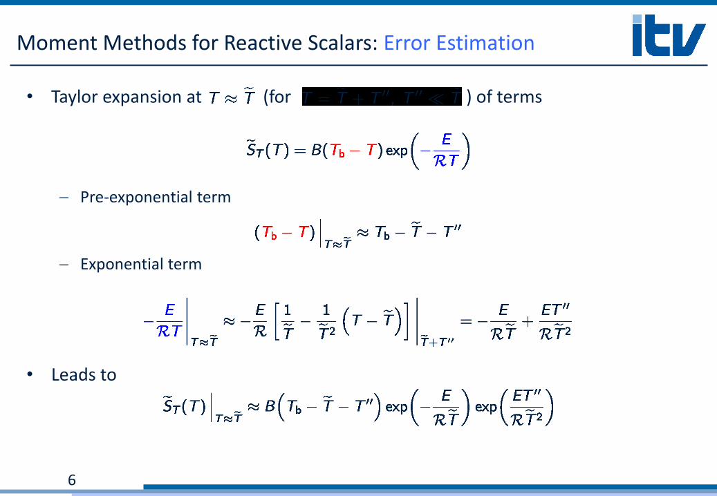
Moment Methods for Reactive Scalars: Error Estimation
• Taylor expansion at (for ) of terms
Pre-exponential term
Exponential term
• Leads to
6

Moment Methods for Reactive Scalars: Error Estimation
• As a function of Favre-mean at yields
• Typical values in the reaction zone of a flame
• Error around a factor of 10!
• Moment method for reactive scalars inappropriate due to strong non-linear effect of the chemical source term
7

Example: Non-Premixed Combustion in Isotropic Turbulence
• Favre averaged transport equation
• Gradient transport model
• One step global reaction
• Decaying isotropic turbulence
8

Example: Non-Premixed Combustion in Isotropic Turbulence
9
Product Mass Fraction
DNS data
Flamelet Closure Assumption
Evaluation of chemical source term with mean quantities
Closure by mean values does not work!

Course Overview
10
• Turbulence
• Turbulent Premixed Combustion
• Turbulent Non-Premixed
Combustion
• Turbulent Combustion Modeling
• Applications
• Moment Methods for reactive scalars
• Simple Models in Fluent: EBU,EDM, FRCM,
EDM/FRCM
• Introduction in Statistical Methods: PDF,
CDF,…
• Transported PDF Model
• Modeling Turbulent Premixed Combustion
• BML-Model
• Level Set Approach/G-equation
• Modeling Turbulent Non-Premixed
Combustion
• Conserved Scalar Based Models for
Non-Premixed Turbulent Combustion
• Flamelet-Model
• Application: RIF, steady flamelet model
Part II: Turbulent Combustion
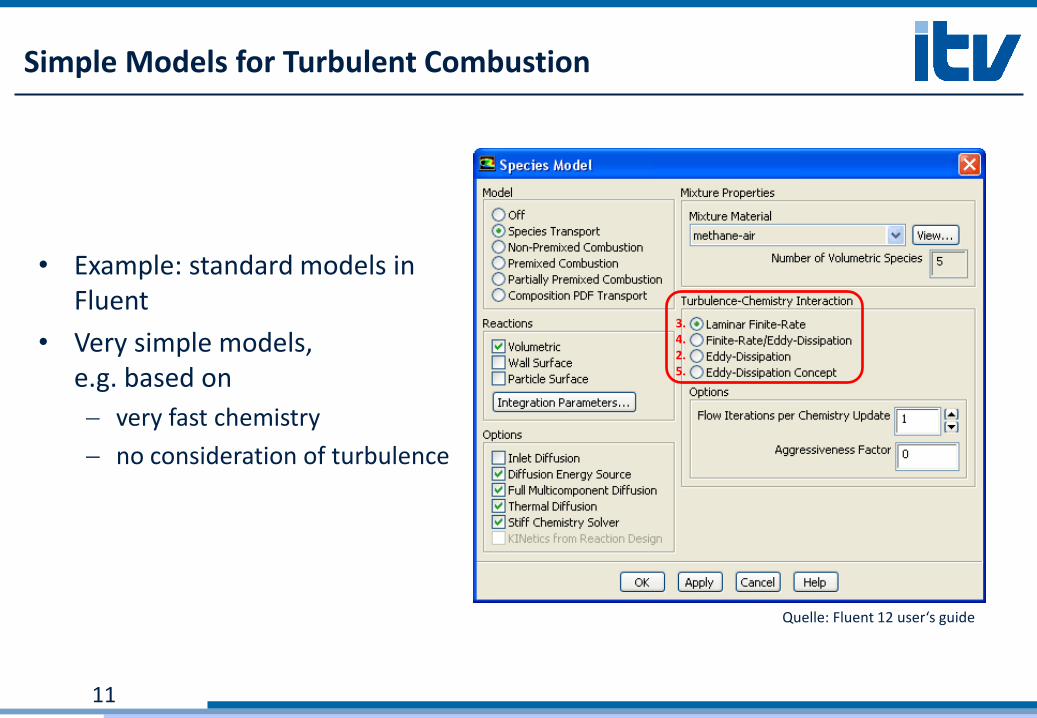
Simple Models for Turbulent Combustion
• Example: standard models in Fluent
• Very simple models, e.g. based on
very fast chemistry
no consideration of turbulence
11
Quelle: Fluent 12 user‘s guide
3. 4. 2. 5.

1. Eddy-Break-Up-Model
First approach for closing the chemical source term was made by Spalding (1971) in premixed combustion
• Assumption: very fast chemistry (after pre-heating)
• Combustion process
Breakup of eddies from the unburnt mixture smaller eddies
→ Large surface area (with hot burnt gas)
→ Duration of this breakup determines the pace
→ Eddy-Break-Up-Model (EBU)
12
flow
hot burnt gas unburnt mixture

1. Eddy-Break-Up-Modell
• Averaged turbulent reaction rate for the products
: variance of mass fraction of the product
CEBU: Eddy-Break-Up constant
• EBU-modell
turbulent mixing sufficiently describes the combustion process
chemical reaction rate is negligible
• Problems with EGR, lean/rich combustion
→ Further development by Magnussen & Hjertager (1977): Eddy-Dissipation-Model (EDM)…
13

2. Eddy-Dissipation-Model
14
• EDM: typical model for eddy breakup
Assumption: very fast chemistry
Turbulent mixing time is the dominant time scale
• Chemical source term
YE, YP: mass fraction of reactant/product
A, B: Model parameter (determined by experiment)

2. Eddy-Dissipation-Model
Example: diffusion flame, one step reaction
• YF > YF,st , therefore YO < YF YE = YO
• YF < YF,st YE = YF
15

Summary EDM
• Controlled by mixing
• Very fast chemistry
• Application: turbulent premixed and nonpremixed combustion
• Connects turbulent mixing with chemical reaction
rich or lean?
→ full or partial conversion
• Advantage: simple and robust model
• Disadvantage
No effects of chemical non-equilibrium (formation of NO, local extinction)
Areas of finite-rate chemistry:
• Fuel consumption is overestimated
• Locally too high temperatures
16

3. Finite-Rate-Chemistry-Model (FRCM)
• Chemical conversion with finite-rate
• Capable of reverse reactions
• Chemical source term for species i in a reaction α
kf,α , kb,α: reaction rates(determined by Arrhenius kinetic expressions )
models the influence of third bodies
• Linearization of the source term centered on the operating point Integration into equations for species, larger Δt realizable
• Typical approach for detailed computation of homogeneous systems
17

Summary FRCM
• Chemistry-controlled
• Appropriate for tchemistry > tmixng (laminar/laminar-turbulent)
• Application
Laminar-turbulent
Non-premixed
• Source term: Arrhenius ansatz
Mean values for temperature in Arrhenius expression
→ Effects of turbulent fluctuations are ignored
→ Temperature locally too low
• Consideration of non-equilibrium effects
18

4. Combination EDM/FRCM
• Turbulent flow
Areas with high turbulence and intense mixing
Laminar structures
• Concept: Combination of EDM and FRCM
For each cell: computation of both reaction rates and
The smaller one is picked (determines the reaction rate)
→ Chooses locally between chemistry- and mixing-controlled
• Advantage: Meant for large range of applicability
• Disadvantage: no turbulence/chemistry interaction
19

5. Eddy-Dissipation-Concept (EDC)
• Extension of EDM Considers detailed reaction kinetics
• Assumption: Reactions on small scales („*“: fine scale)
• Volume of small scales:
• Reaction rates are determined by Arrhenius expression (cf. FRCM)
• Time scale of the reactions
20
Fluent: Cξ = 2,1377
Fluent: Cτ = 0,4082

5. Eddy-Dissipation-Concept (EDC)
• Boundary/initial conditions for reactions (on small scales)
Assumption: pressure p = const.
Initial condition: temperature and species concentration in a cell
Reactions on time scale
Numerical integration (e.g. ISAT-Algorithm)
• Model for source term
• Problem:
Requires a lot of processing power
Stiff differential equation
21
Mass fraction on small scales of species i after reaction time τ*

Summary: Simple Combustion Models
22
Quelle: Fluent 12 user‘s guide
3. 4. 2. 5.
Solely calculation by Arrhenius equation turbulence is not considered
Calculation of Arrhenius reaction rate and mixing rate; selection of the smaller one local choice: laminar/turbulent
Solely calculation of mixing rate Chemical kinetic is not considered
Modeling of turbulence/chemistry interaction; detailed chemistry

Course Overview
23
• Turbulence
• Turbulent Premixed Combustion
• Turbulent Non-Premixed
Combustion
• Turbulent Combustion Modeling
• Applications
• Moment Methods for reactive scalars
• Simple Models in Fluent: EBU,EDM, FRCM,
EDM/FRCM
• Introduction in Statistical Methods: PDF,
CDF,…
• Transported PDF Model
• Modeling Turbulent Premixed Combustion
• BML-Model
• Level Set Approach/G-equation
• Modeling Turbulent Non-Premixed
Combustion
• Conserved Scalar Based Models for
Non-Premixed Turbulent Combustion
• Flamelet-Model
• Application: RIF, steady flamelet model
Part II: Turbulent Combustion

Introduction to Statistical Methods
• Introduction to statistical methods
Sample space
Probability
Cumulative distribution function(CDF)
Probability density function(PDF)
Examples for CDFs/PDFs
Moments of a PDF
Joint statistics
Conditional statistics
24
Pope, „Turbulent Flows“

• Probability of events in sample space
• Sample space: set of all possible events
Random variable U
Sample space variable V (independent variable)
• Event A
• Event B
Sample Space
25

Probability
• Probability of the event
• Probability p
26
impossible event sure event
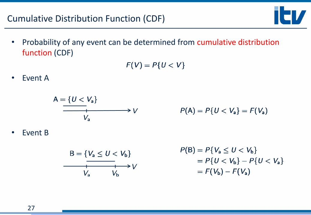
Cumulative Distribution Function (CDF)
• Probability of any event can be determined from cumulative distribution function (CDF)
• Event A
• Event B
27

Cumulative Distribution Function (CDF)
• Three basic properties of a CDF
1. Occuring of event is impossible
2. Occuring of event is sure
3. F is a non-decreasing function as
28
CDF of Gaussian distributed random variable

Probability Density Function (PDF)
• Derivative of the CDF probability density function
• Three basic properties of a PDF
1. CDF non-decreasing PDF
2. Satisfies the normalization condition
3. For infinite sample space variable
29
PDF of Gaussian distributed random variable

Probability Density Function (PDF)
• Examining the particular interval Va ≤ U < Vb
• Interval Vb - Va 0:
30

Example for CDF/PDF
Uniform distribution
31
Source: Pope, „Turbulent Flows“

Example for CDF/PDF
32
Source: Pope, „Turbulent Flows“
Exponential distribution

Example for CDF/PDF
33
Source: Pope, „Turbulent Flows“
Normal distribution

Example for CDF/PDF
34
Source: Pope, „Turbulent Flows“
or
Delta-function distribution
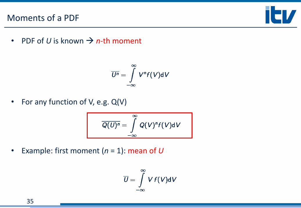
Moments of a PDF
• PDF of U is known n-th moment
• For any function of V, e.g. Q(V)
• Example: first moment (n = 1): mean of U
35

Central Moments
• n-th central moment
• Example: second central moment (n = 2): variance of U
36

Joint Cumulative Density Function
• Joint CDF (jCDF) of random variables U1, U2 (in general Ui, i = 1,2,…)
37
Source: Pope, „Turbulent Flows“

Joint Cumulative Density Function
• Basic properties of a jCDF
Non-decreasing function
Since is impossible
Since is certain equally
38
marginal CDF

Joint Probability Density Function
• Joint PDF (jPDF)
• Fundamental property:
39
Source: Pope, „Turbulent Flows“

Joint Probability Density Function
• Basic properties of a jPDF
Non-negative:
Satisfies the normalization condition
Marginal PDF
40

Joint Statistics
• For a function Q(U1,U2,…)
From joint pdf of V, all moments can be obtained for all functions of V
• Example: i = 1, 2; n = 1; , covariance of U1 and U2
Covariance shows the correlation of two variables
41
Scatterplot of two velocity- components U1 and U2
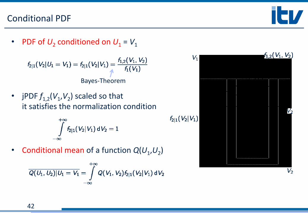
Conditional PDF
• PDF of U2 conditioned on U1 = V1
• jPDF f1,2(V1,V2) scaled so that it satisfies the normalization condition
• Conditional mean of a function Q(U1,U2)
42
Bayes-Theorem

Statistical Independence
• If U1 and U2 are statistically independent, conditioning has no effect
• Bayes-Theorem
• Therefore:
• Independent variables uncorrelated
• In general the converse is not true
43

Course Overview
44
• Turbulence
• Turbulent Premixed Combustion
• Turbulent Non-Premixed
Combustion
• Turbulent Combustion Modeling
• Applications
• Moment Methods for reactive scalars
• Simple Models in Fluent: EBU,EDM, FRCM,
EDM/FRCM
• Introduction in Statistical Methods: PDF,
CDF,…
• Transported PDF Model
• Modeling Turbulent Premixed Combustion
• BML-Model
• Level Set Approach/G-equation
• Modeling Turbulent Non-Premixed
Combustion
• Conserved Scalar Based Models for
Non-Premixed Turbulent Combustion
• Flamelet-Model
• Application: RIF, steady flamelet model
Part II: Turbulent Combustion

• Models based on a pdf transport equation for velocity and reactive scalars are usually
formulated for one-point statistics
One-point/multi-variable joint statistics
• A transport equation for joint probability density function P(v, ψ ; x, t) of velocity v
and all reactive scalars ψ can be derived (cf. O'Brien, 1980; Pope, 1985, 2000)
where is gradient with respect to velocity components, angular brackets are
conditional means, and the same symbol is used for random and sample space variables
The PDF Transport Equation Model
45
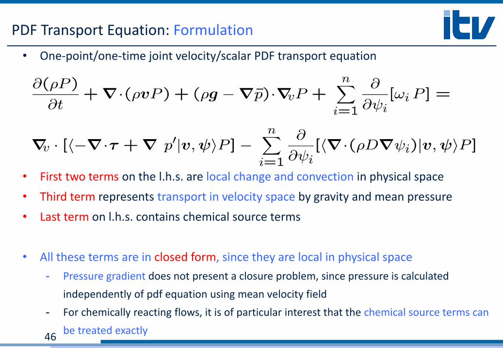
• One-point/one-time joint velocity/scalar PDF transport equation
• First two terms on the l.h.s. are local change and convection in physical space
• Third term represents transport in velocity space by gravity and mean pressure
• Last term on l.h.s. contains chemical source terms
• All these terms are in closed form, since they are local in physical space
- Pressure gradient does not present a closure problem, since pressure is calculated
independently of pdf equation using mean velocity field
- For chemically reacting flows, it is of particular interest that the chemical source terms can
be treated exactly
PDF Transport Equation: Formulation
46

• First unclosed term on r.h.s. describes transport of PDF in velocity space induced by
viscous stresses and fluctuating pressure gradient
• Second term represents transport in reactive scalar space by molecular fluxes
This term represents molecular mixing and is unclosed
PDF Transport Equation: Closure Problem
47
• One-point/one-time joint velocity/scalar PDF transport equation

• For fast chemistry, mixing and reaction take place in thin layers where molecular transport
and the chemical source term balance each other
- Hence, closed chemical source term and unclosed molecular mixing term are closely
linked to each other
- Pope and Anand (1984) have illustrated this for the case of premixed turbulent
combustion by comparing a standard pdf closure for the molecular mixing term with
a formulation, where the molecular diffusion term was combined with the chemical
source term to define a modified reaction rate
- They call the former distributed combustion and the latter flamelet combustion and
find considerable differences in the Damköhler number dependence of the turbulent
burning velocity normalized with the turbulent intensity
PDF Transport Equation: Fast chemistry
48

• PDF transport equation is scalar equation in many dimensions
- Mesh-based techniques not attractive for high-dimensional equations
→ Monte-Carlo simulation techniques (cf. Pope, 1981, 1985)
• Monte-Carlo methods represent PDF by large number of so-called notional particles
- Particles should be considered different realizations of turbulent reactive flow
- Statistical error decreases with N1/2
→ Slow convergence
• Application mostly only for joint scalar PDF coupled with Eulerian RANS flow solver
- Coupling between Lagrangian and Eulerian solver important
• Applications often in steady RANS
Large particle number achieved by time averaging
PDF Transport Equation: Application
49

PDF Transport Equation: Application in LES
50
• Density weighted joined scalar filtered density function FL (FDF) defined using filter kernel G
• Note: FDF does not have the statistical properties as a PDF
• Challenges:
- LES is unsteady
→ Large number of notional particles required in each cell at each point in time
- Keep number of particles per cell uniform
- Two-way conservative interpolation between particles and mesh
- Large number of cells makes chemistry integration even more expensive
→ In situ adaptive tabulation
- Eulerian/Lagrangian coupling needs to be achieved at all times

Application TPDF Model in LES of Turbulent Jet Flames
• LES/FDF of Sandia flames D and E (Raman & Pitsch, 2007)
Joint scalar pdf
Eulerian/Lagrangian coupling
→ Density computed through filtered enthalpy equation for improve numerical stability
Detailed chemical mechanism (19 species)
30-50 particles per cell
Simple mixing model (Interaction by exchange with the mean, IEM)
• Mixing time needs to be modeled Usually tf = tt / Cf where Cf = const
• Here, new dynamic model for Cf
Modeled stochastic differential equation for particle-position
51
1 V. Raman and H. Pitsch, A consistent LES/filtered-density function formulation for the simulation of turbulent flames with detailed chemistry, Proc. Comb. Inst., 31, pp. 1711–1719, 2007.

Application TPDF Model in LES of Turbulent Jet Flames
52
Flame D: Temperature
Flame E: Temperature
Flame E: Dissipation Rate

Application TPDF Model in LES of Turbulent Jet Flames
53

Course Overview
54
• Turbulence
• Turbulent Premixed Combustion
• Turbulent Non-Premixed
Combustion
• Turbulent Combustion Modeling
• Applications
• Moment Methods for reactive scalars
• Simple Models in Fluent: EBU,EDM, FRCM,
EDM/FRCM
• Introduction in Statistical Methods: PDF,
CDF,…
• Transported PDF Model
• Modeling Turbulent Premixed Combustion
• BML-Model
• Level Set Approach/G-equation
• Modeling Turbulent Non-Premixed
Combustion
• Conserved Scalar Based Models for
Non-Premixed Turbulent Combustion
• Flamelet-Model
• Application: RIF, steady flamelet model
Part II: Turbulent Combustion

Bray-Moss-Libby-Model
• Flamelet concept for premixed turbulent combustion: Bray-Moss-Libby-Model (BML)
• Premixed combustion: progress variable c, e.g.
• Favre averaged transport equation (neglecting the molecular transport)
• Closure for turbulent transport and chemical source term by BML-Model
55
not closed
or

Bray-Moss-Libby-Model
• Assumption: very fast chemistry, flame size lF << η << lt
• Fuel conversion only in the area of thin flame front → in the flow field
Burnt mixture or
Unburnt mixture,
Intermediate states are very unlikely
56
burnt burnt
unburnt

• Assumption: progress variable is expected solely to be c = 0 (unburnt) or c = 1 (burnt)
• Probability densitiy function
: probabilities, to encounter burnt or unburnt mixture in the flow field
No intermediate states
δ: Delta function
Bray-Moss-Libby-Model
57

Bray-Moss-Libby-Model
58
instantaneous flame front
mean flame front
„unburnt“ „burnt“

BML-closure of Turbulent Transport
• For a Favre average
• Therefore the unclosed correlation
joint PDF for u and c
Introducing the BML approach for f(c) leads to
59
conditional PDF delta function
(Bayes-Theorem)

BML-closure of Turbulent Transport
• With follows
60

Bray-Moss-Libby-Model: „countergradient diffusion“
• Because of ρu = const. through flame front: u↑ just as much as ρ↓
• Because of c ≥ 0
• Within the flame zone
• Gradient transport assumption would be
• Conflict: „countergradient diffusion“
61
Flame front
uu ub
ρuuu = ρbub
c
conflict

BML-closure of Chemical Source Term
• Closure by BML-model f(c) leads to
• Closure of the chemical source term, e.g. by flame-surface-density-model
I0: strain factor local increase of burning velocity by strain
• Flame-surface-density Σ
e.g. algebraic model:
Or transport equation for Σ
62
local mass conversion per area
Flächen-Dichte (flamen area per volume)
Flame crossing length

BML-closure of Chemical Source Term
• Transport equation for Σ
• No chemical time scale
Turbulent time (τ = k/ε) is the determining time scale
Limit of infinitely fast chemistry
By using transport equations model for chemical source term independent of sL
63
local change
convectiv change
turbulent transport
production due to stretching of the flame
flame- annihilation

Course Overview
64
• Turbulence
• Turbulent Premixed Combustion
• Turbulent Non-Premixed
Combustion
• Turbulent Combustion Modeling
• Applications
• Moment Methods for reactive scalars
• Simple Models in Fluent: EBU,EDM, FRCM,
EDM/FRCM
• Introduction in Statistical Methods: PDF,
CDF,…
• Transported PDF Model
• Modeling Turbulent Premixed Combustion
• BML-Model
• Level Set Approach/G-equation
• Modeling Turbulent Non-Premixed
Combustion
• Conserved Scalar Based Models for
Non-Premixed Turbulent Combustion
• Flamelet-Model
• Application: RIF, steady flamelet model
Part II: Turbulent Combustion

Level-Set-Approach
• Kinematics of the flame front by examining the movement of single flame front-„particles“
• Movement influenced by
Local flow velocity ui, i = 1,2,3
Burning velocity sL
65
normal vector
instantaneous flame front
particle

G-Equation
• Instead of observing a lot of particles examination of a scalar field G
• Iso-surface G0 is defined as the flame front
• Substantial derivative of G (on the flame front)
66
unburnt burnt

G-Equation for Premixed Combustion
• Kinematics and lead to
→ G-Equation for premixed combustion
67
normal vector
unburnt burnt

G-Equation in the Regime of Corrugated Flamelets
• No diffusive term
• Can be applied for
Thin flames
Well-defined burning velocity
→ Regime of corrugated flamelets (η >> lF >> lδ)
68
local change
convective change
progress of flame front by burning velocity
unburnt burnt

G-Equation in the Regime of Corrugated Flamelets
• Kinematic equation ≠ f(ρ)
• Valid for flame position: G = G0 (= 0)
For solving the field equation, G needs to be defined in the entire field
Different possibilities to define G, e.g. signed distance function
69
unburnt burnt

G-Equation in the Regime of Corrugated Flamelets
• Influence of chemistry by sL
• sL not necessarily constant, influenced by strain S
curvature κ
Lewis number effect
• Modified laminar burning velocity
70
unburnt burnt

Laminar Burning Velocity: Curvature
71
influence of curvature
uncorrected laminar burning velocity
unburnt G < 0
burnt G > 0

Laminar Burning Velocity: Markstein Length
• Markstein length
Determined by experiment
Or by asymptotic analysis
72
density ratio
Zeldovich number Lewis number
uncorrected laminar burning velocity

Extended G-Equation
→ Extended G-Equation
73
influence of strain
influence of curvature
Markstein length
uncorrected laminar burning velocity

G-Equation: Corrugated Flamelets/Thin Reaction Zones
• Previous examinations limited to the regime of corrugated flamelets
Thin flame structures (η >> lF >> lδ)
Laminar burning velocity well-defined
• Regime of thin reaction zones
Small scale eddies penetrate the preheating zone
Transient flow
Burning velocity not well-defined
→ Problem: Level-Set-Approach valid in the regime of thin reaction zones?
74
no longer valid

G-Equation: Regime of Thin Reaction Zones
• Assumption: „G=0“ surface is represented by inner reaction zone
• Inner reaction zone
Thin compared to small scale eddies, lδ << η
Described by T(xi,t) = T0
• Temperature equation
• Iso temperature surface T(xi,t) = T0
75

G-Equation: Regime of Thin Reaction Zones
• Equation of motion of the iso temperature surface T(xi,t) = T0
With the displacement speed sd
Normal vector
76

G-Equation: Regime of Thin Reaction Zones
• With G0 = T0
Diffusion term normal diffusion (~sn) and curvature term (~κ)
→ G-equation for the regime of thin reaction zones
77

Common Level Set Equation for Both Regimes
• Normalize G-equation with Kolmogorov scales (η, τη, uη) leads to
78

Order of Magnitude Analysis
• Non dimensional
→ Derivatives, ui*, κ* ≈ O(1)
• Typical flame
→ Sc = ν/D ≈ 1 D/ν = O(1)
• Parameter: sL/uη
Ka = uη2/sL
2 sL/uη = Ka-1/2
sL,s ≈ sL
79
O(Ka-1/2) O(1)

G-Equation for both Regimes
• Thin reaction zones: Ka >> 1 curvature term is dominant
• Corrugated flamelets: Ka << 1 sL term is dominant
• Leading order equation in both regimes
80
O(Ka-1/2) O(1)
Assumption: const. const.
Statistical Description of Turbulent Flame Front
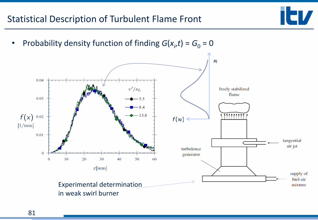
• Probability density function of finding G(xi,t) = G0 = 0
81
Experimental determination in weak swirl burner

Statistical Description of Turbulent Flame Front
• Consider steady one-dimensional premixed turbulent mean flame at position xf
• Define flame brush thickness lf from f(x)
• If G is distance function then
82

Favre-Mean- and Variance-Equation
• Equation for Favre-mean
• Equation for variance
• can be interpreted as the area ratio of the flame AT/A
• Variance describes the average size of the flame
83
instantaneous flame front
averaged flame front
averaged temperature profile
instantaneous temperature profile

Modeling of the Variance Equation
• Sink terms in the variance equation
Kinematic restoration
Scalar dissipation
are modeled by
84
G-Equation for Turbulent Flows
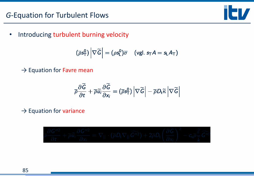
• Introducing turbulent burning velocity
→ Equation for Favre mean
→ Equation for variance
85

G-Equation for Turbulent Flows
• Modeling of turbulent burning velocity by Damköhler theory
86

G-Equation for Turbulent Flows
• Favre mean of G
• Favre-PDF
• Mean temperature (or other scalar)
87
T(G)=T(x) taken from laminar premixed flame without strain
instantaneous flame front
averaged flame front
averaged temperature profile
instantaneous temperature profile

Example: Presumed Shape PDF Approach (RANS)
88
experiment
computed numerically

G-Equation for LES
• Different averaging procedure1
• Start from progress variable C defined from temperature or reaction products
• Equation for Heaviside function centered at C = C0
• With where
89
1 E. Knudsen and H. Pitsch, A dynamic model for the turbulent burning velocity for large eddy simulation of premixed combustion, Combust. Flame, 154 (4), pp. 740–760, 2008.

G-Equation for LES
• Filtered Heaviside function
• Modeled equation for filtered Heaviside function describes evolution of filtered front, but cannot be adequately resolved in LES
• Introduce level set function describing filtered front evolution gives level set equation for filtered flame front
90

• Premixed methan/air flame
• Re = 23486
• Broad, low velocity pilot flame heat losses to burner
• Dilution by air co-flow
91
Example: LES of a Premixed Turbulent Bunsen Flame
temperature
axial velocity

Time-Averaged Temperature and Axial Velocity at position x/D = 2.5
92
temperature axial velocity
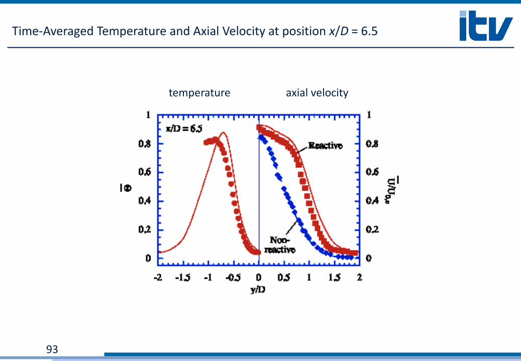
Time-Averaged Temperature and Axial Velocity at position x/D = 6.5
93
temperature axial velocity

Turbulent Kinetic Energie at Position x/D = 2.5 and 6.5
94
x/D = 2,5 x/D = 6,5
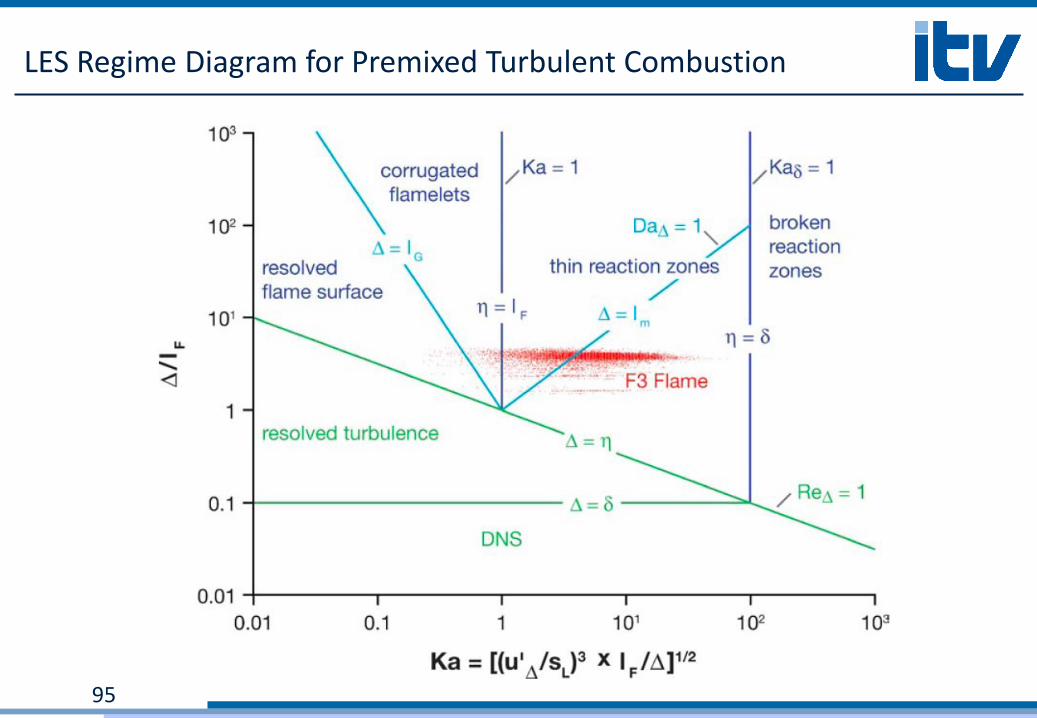
LES Regime Diagram for Premixed Turbulent Combustion
95

Course Overview
96
• Turbulence
• Turbulent Premixed Combustion
• Turbulent Non-Premixed
Combustion
• Turbulent Combustion Modeling
• Applications
• Moment Methods for reactive scalars
• Simple Models in Fluent: EBU,EDM, FRCM,
EDM/FRCM
• Introduction in Statistical Methods: PDF,
CDF,…
• Transported PDF Model
• Modeling Turbulent Premixed Combustion
• BML-Model
• Level Set Approach/G-equation
• Modeling Turbulent Non-Premixed
Combustion
• Conserved Scalar Based Models for
Non-Premixed Turbulent Combustion
• Flamelet-Model
• Application: RIF, steady flamelet model
Part II: Turbulent Combustion

Mixture Fraction Z
• Assume
One-step global reaction: nF F + nO O nP P
Lei = 1
• Species transport and temperature equations
• With follows
97

Mixture Fraction Z
• Derive coupling function b by eliminating w such that
• With and follows
• Normalization between 0 and 1 gives
98

Transport Equation for Z
• Transport equation
Advantage: L(Z) = 0 No Chemical Source Term
BC: Z = 0 in Oxidator, Z = 1 in Fuel
• If species and temperature function of mixture fraction, then
• Needed:
Local statistics of Z (expressed by PDF)
Species/temperature as function of Z: Yi(Z) and T(Z)
99

Presumed PDF Approach
• Equation for the mean and the variance of Z are known and closed
100

Presumed PDF Approach
• b-function pdf for mixture fraction Z
• With
101

Conserved Scalar Based Models for Non-Premixed Turbulent Combustion
• Infinitely fast irreversible chemistry
Burke-Schumann solution
Solution = f(Z)
• Infinitely fast reversible chemistry
Chemical equilibrium
Solution = f(Z)
• Flamelet model for non-premixed combustion
Chemistry fast, but not infinitely fast
Solution = f(Z, χ)
• Conditional Moment Closure (CMC)
Similar to flamelet model
Solution = f(Z,< χ|Z>)
102

Conserved Scalar Based Models for Non-Premixed Turbulent Combustion
• Infinitely fast irreversible chemistry
Burke-Schumann solution
Solution = f(Z)
• Infinitely fast reversible chemistry
Chemical equilibrium
Solution = f(Z)
103

Burke-Schumann Solution
104

Course Overview
105
• Turbulence
• Turbulent Premixed Combustion
• Turbulent Non-Premixed
Combustion
• Turbulent Combustion Modeling
• Applications
• Moment Methods for reactive scalars
• Simple Models in Fluent: EBU,EDM, FRCM,
EDM/FRCM
• Introduction in Statistical Methods: PDF,
CDF,…
• Transported PDF Model
• Modeling Turbulent Premixed Combustion
• BML-Model
• Level Set Approach/G-equation
• Modeling Turbulent Non-Premixed
Combustion
• Conserved Scalar Based Models for
Non-Premixed Turbulent Combustion
• Flamelet-Model
• Application: RIF, steady flamelet model
Part II: Turbulent Combustion

Flamelet Model for Non-Premixed Turbulent Combustion
• Basic idea: Scale separation
• Assume fast, but not infinitely fast chemistry: 1 << Da << ∞
• Reaction zone is thin compared to small scales of turbulence and hence retains laminar structure
• Transformation and asymptotic approximation leads to flamelet equations
106

Flamelet Model for Non-Premixed Turbulent Combustion
• Balance equations for temperature, species and mixture fraction
• With it follows
107

Flamelet Equations
• Consider surface of stoichiometric mixture
• Reaction zone confined to thin layer around this surface
• Transformation to surface attached coordinate system
• x1, x2, x3, t → Z(x1, x2, x3, t), Z2, Z3, τ
108
x1, Z
x2, Z2
x3, Z3

Transformation rules
• Transformation: x1, x2, x3, t → Z(x1, x2, x3, t), Z2, Z3, τ (where Z2 = x2 , Z3 = x3, τ = t)
• Example: Temperature T
109
0 0 1
0 0 0
0 0
Analogous for x3
1

Flamelet Equations
• Temperature equation Transformed temperature equation:
110

• If the flamelet is thin in the Z direction, an order-of-magnitude analysis similar to that for a boundary layer shows that is the dominating term of the spatial derivatives
• Equivalent to the assumption that temperature derivatives normal to the flame surface are much larger than those in tangential direction
• ∂T/∂τ is important if very rapid changes, such as extinction, occur
Flamelet Equations
111
small
Local change Describes mixing
Source term
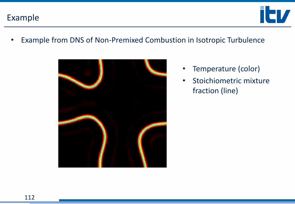
Example
• Example from DNS of Non-Premixed Combustion in Isotropic Turbulence
112
• Temperature (color)
• Stoichiometric mixture fraction (line)

Flamelet Equations
• Same procedure for the mass fraction…
• Flamelet structure is to leading order described by the one-dimensional time-dependent equations
→
• Instantaneous scalar dissipation rate at stoichiometric conditions
→ [χst] = 1/s: may be interpreted as the inverse of a characteristic diffusion time
113

Temperature profiles for methane-air flames
• Temperature profiles for methane-air flames
114
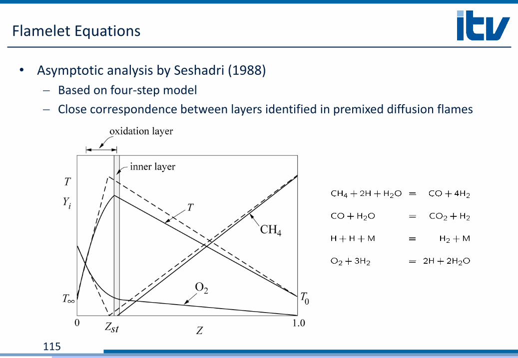
Flamelet Equations
• Asymptotic analysis by Seshadri (1988)
Based on four-step model
Close correspondence between layers identified in premixed diffusion flames
115

Flamelet Equations
• The calculations agree well with numerical and experimental data
• They also show the vertical slope of T0 versus χst which corresponds to extinction
116

Flamelet Equations
• Steady state flamelet equations provide ψi = f(Z,χst)
• If joint pdf is known
→ Favre mean of ψi:
• If the unsteady term in the flamelet equation must be retained, joint statistics of Z and χst become impractical
• Then, in order to reduce the dimension of the statistics, it is useful to introduce multiple flamelets, each representing a different range of the χ-distribution
• Such multiple flamelets are used in the Eulerian Particle Flamelet Model (EPFM) by Barths et al. (1998)
• Then the scalar dissipation rate can be formulated as function of the mixture fraction
117

Flamelet Equations
• Modeling the conditional Favre mean scalar dissipation rate
• Flamelet equations
• Favre mean
118

Flamelet Equations
• Model for conditional scalar dissipation rate
• One relates the conditional scalar dissipation rate to that at a fixed value Zst by
With
119
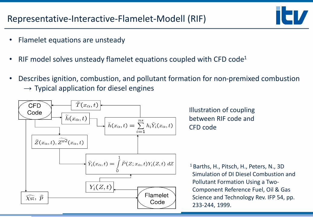
Representative-Interactive-Flamelet-Modell (RIF)
120
• Flamelet equations are unsteady
• RIF model solves unsteady flamelet equations coupled with CFD code1
• Describes ignition, combustion, and pollutant formation for non-premixed combustion
→ Typical application for diesel engines
Illustration of coupling between RIF code and CFD code
1 Barths, H., Pitsch, H., Peters, N., 3D Simulation of DI Diesel Combustion and Pollutant Formation Using a Two-Component Reference Fuel, Oil & Gas Science and Technology Rev. IFP 54, pp. 233-244, 1999.

n-Heptane Air Ignition
• The initial air temperature is 1100 K and the initial fuel temperature is 400 K.
121

Example: Diesel engine simulation
• VW 1,9 l DI-Diesel engine (Fuel: n-Heptan)
• Simulation:
KIVA-Code
RIF-Model
n-Heptan detailed chemistry
Soot and Nox as function of EGR
122

Example: Diesel engine simulation
• RIF-Temperature
123
0.00.2
0.40.6
0.81.0
Mischungsbruch -10
0
10
20
Kurbelwinkel [˚nOT]
300
600
900
1200
1500
1800
2100
2400
2700
T [K]
300 600 900 1200 1500 1800 2100 2400 2700
Temperatur [K]

Example: Diesel engine simulation
124
Mischungsbruch- verteilung
Schadstoff- bildung

Example: Diesel engine simulation
• Comparison with Magnussen-/ Hiroyasu-Model
125

Example: ITV Diesel Engine Test Bench
• The range of operation was extended for partially homogenized conditions (PCCI)
• High performance measurement equipment
• Rapid and dynamic measurement of EGR
• Fast sensors with cycle-to-cycle resolution for NOx and uHC
• Stationary measurement of soot, CO, CO2, ...
Engine type 4 cylinder diesel engine
Bore 82.0 mm
Stroke 90.4 mm
Displacement 1910 mm³
Pistons Reentrant type
Compression ratio 17.5:1
Valves 16 V
Max. Power 110 kW (150 PS)
Swirl number 2.5
Injection system Bosch Common-Rail (2nd generation),
central injector position,
7 holes nozzle

Numerical Setup
•Multidimensional CFD-RANS code AC-FLuX
•Computations performed for variations in
– Start of energizing (SOE): 10, 20, 30, 40 and 50 deg CA bTDC
– Fuel mass injected (FMI): 11, 12, 13.5 and 17.5 mm3/cycle
– Exhaust gas recirculation (EGR): 0, 15, 26, 33 and 34 %
•Computations from IVC to EVO
•Sector grid of the combustion chamber (~ 50000 cells)
•Two different meshes for compression and combustion
•RIF combustion model initialized at start of injection

Multi-Zone Model Results
• Scalar dissipation rate: • Strong influence of SOE on position and maximum • FMI and EGR only affect the maximum value • IMEP: • Good qualitative agreement • Noticeable deviation at SOE 50 • CA50: • Even better agreement • Only minor deviations observable

Results
• Good agreement in terms of in-cylinder pressure
• Ignition delay
• Combustion
• Peak pressure
• Expansion
• Nitrogen oxides (NOx) and unburned hydrocarbons (HC):
• Simulation captures experimental trend
• Minor deviations for latest injection timing (NOx) and early injection timings (HC)

Injector cut plane SOE 40
Top dead center
40 deg CA aTDC

Injector cut plane SOE 50
Top dead center
40 deg CA aTDC HC-Emissions

Flamelet Models for Turbulent Combustion

Multi-D Flamelet Models for Turbulent Combustion
• 3

Multi-D Flamelet Models for Turbulent Combustion

Multi-D Flamelet Models for Turbulent Combustion

Example: High Fidelity Modeling of Multi-Injection Diesel Engine Application
136

Solver and Modeling Approaches
137 [1] S. Liu, J.C. Hewson, J.H. Chen, and H. Pitsch, Combustion and Flame, 2004

Close Pilot Injection
• Close pilot injection:
• IMEP: 8 bar
• 28% EGR
138

Classic Pilot Injection
• Classic pilot injection:
– IMEP: 8 bar
– 24% EGR
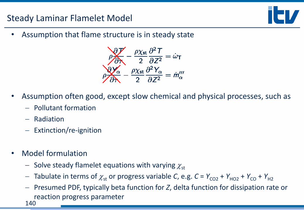
Steady Laminar Flamelet Model
• Assumption that flame structure is in steady state
• Assumption often good, except slow chemical and physical processes, such as
Pollutant formation
Radiation
Extinction/re-ignition
• Model formulation
Solve steady flamelet equations with varying cst
Tabulate in terms of cst or progress variable C, e.g. C = YCO2 + YHO2 + YCO + YH2
Presumed PDF, typically beta function for Z, delta function for dissipation rate or reaction progress parameter
140

• Bluff-body stablized methane/air flame
• Fuel issues through center of bluff body
• Flame stabilization by complex recirculating flow
• RANS models where unsuccessful in predicting
experimental data
• Here, LES using simple steady flamelet model
• New recursive filter refinement method
• Accurate models for scalar variance and scalar
dissipation rate
Example: LES of a Bluff-Body Stabilized Flame
141
Exp. by Masri et al.

Example: LES of a Bluff-Body Stabilized Flame
142

Temperature CO Mass Fraction
Example: LES of a Bluff-Body Stabilized Flame
143

Flamelet Model Application to Sandia Jet Flames
Flamelet model application to jet flame with extinction and reignition
• Flamelet/progress variable model (Ihme & Pitsch, 2008)
• Definition of reaction progress parameter
Based on progress variable C
Defined to be independent of Z
• Joint pdf of Z and l
Z and l independent
Beta function for Z
Statistically most likely distribution for l
144
Exp. by Barlow et al.

Flamelet Model Application to Sandia Jet Flames
145
Flame D: Temperature
Flame E: Temperature

Flamelet Model Application to Sandia Jet Flames
146
Flame E
Flame D
Flame E
Flame D

Summary
147
• Turbulence
• Turbulent Premixed Combustion
• Turbulent Non-Premixed
Combustion
• Turbulent Combustion Modeling
• Applications
• Moment Methods for reactive scalars
• Simple Models in Fluent: EBU,EDM, FRCM,
EDM/FRCM
• Introduction in Statistical Methods: PDF,
CDF,…
• Transported PDF Model
• Modeling Turbulent Premixed Combustion
• BML-Model
• Level Set Approach/G-equation
• Modeling Turbulent Non-Premixed
Combustion
• Conserved Scalar Based Models for
Non-Premixed Turbulent Combustion
• Flamelet-Model
• Application: RIF, steady flamelet model
Part II: Turbulent Combustion