COLOR-BASED MODELS FOR OUTDOOR MACHINE VISION A ...

COLOR-BASED MODELS FOR OUTDOOR MACHINE VISION

A Dissertation Presented

by

SHASHI D. BULUSWAR

Submitted to the Graduate School of

The University of Massachusetts Amherst in partial fulfillment of the requirements for the degree of

DOCTOR OF PHILOSOPHY

February, 2002

Department of Computer Science


A Dissertation Presented

by

Shashi D. Buluswar Approved as to style and content by: _____________________________________________ Allen R. Hanson, Chair _____________________________________________ Bruce A. Draper, Member _____________________________________________ Edward M. Riseman, Member _____________________________________________ Andrew G. Barto, Member _____________________________________________ Michael Skrutskie, Member

____________________________________ Bruce Croft, Department Chair Computer Science

ABSTRACT


FEBRUARY, 2002

SHASHI D. BULUSWAR, B.A., GOSHEN COLLEGE

M.S., UNIVERSITY OF MASSACHUSETTS AMHERST

Ph.D., UNIVERSITY OF MASSACHUSETTS AMHERST

Directed by: Professor Allen R. Hanson

This study develops models for illumination and surface reflectance for use in

outdoor color vision, and in particular for predicting the color of surfaces under outdoor

conditions. Existing daylight and reflectance models that have been the basis for much of

color research thus far have certain limitations that reduce their applicability to outdoor

machine vision imagery. In that context, this work makes three specific contributions: (i)

an explanation of why the current standard CIE daylight model cannot be used to predict

the color of light incident on surfaces in machine vision images, (ii) a model (table)

mapping the color of daylight to a broad range of sky conditions, and (iii) a simplified

adaptation of the frequently used Dichromatic Reflectance Model for use with the

developed daylight model. A series of experiments measure the accuracy of the daylight

and reflectance models by predicting the colors of surfaces in real images. Finally, a

series of tests demonstrate the potential use of these methods in outdoor applications such

as road-following and obstacle detection.

iv

v

TABLE OF CONTENTS

Page

ABSTRACT....................................................................................................................... iv

LIST OF TABLES ...........................................................................................................viii

LIST OF FIGURES............................................................................................................ ix CHAPTER

1. INTRODUCTION....................................................................................................... 1

1.1 Overview ........................................................................................................... 1 1.2 Variation of apparent color ............................................................................... 2 1.3 Overview of chapters ........................................................................................ 7

2. FACTORS IN OUTDOOR COLOR IMAGES ........................................................ 10

2.1 Overview ......................................................................................................... 10 2.2 Light, the visual spectrum, and color .............................................................. 10 2.3 The effect of illumination................................................................................ 13 2.4 The effect of surface orientation and reflectance ............................................ 17 2.5 The effect of the sensor ................................................................................... 18 2.6 Shadows and inter-reflections ......................................................................... 23

3. PREVIOUS WORK.................................................................................................. 26

3.1 Overview ......................................................................................................... 26 3.2 Color machine vision ...................................................................................... 26

3.2.1 Color constancy ................................................................................ 27 3.2.2 Parametric classification................................................................... 30 3.2.3 Techniques based on machine-learning............................................ 30 3.2.4 Color segmentation........................................................................... 31 3.2.5 Color indexing .................................................................................. 32

3.3 Models of daylight .......................................................................................... 32 3.4 Surface reflectance models.............................................................................. 33

4. A MODEL OF OUTDOOR COLOR ....................................................................... 36

4.1 Overview ......................................................................................................... 36 4.2 The CIE daylight model .................................................................................. 37 4.3 Daylight in machine vision images ................................................................. 38

vi

4.3.1 Incident light from the direction away from the sun ........................ 43 4.3.2 Incident light in the direction of the sun........................................... 54

4.4 Daylight color indexed by context .................................................................. 55

5. A SURFACE REFLECTANCE MODEL: THE NPF .............................................. 59

5.1 Overview ......................................................................................................... 59 5.2 Existing physics-based models........................................................................ 60 5.3 Derivation of the NPF ..................................................................................... 65 5.4 The photometric function ................................................................................ 71

5.4.1 Empirically obtaining the NPF for particular surfaces ..................... 72

6. ESTIMATING APPARENT NORMALIZED COLOR........................................... 83

6.1 Overview ......................................................................................................... 83 6.2 Estimating apparent color when the relative viewing angle is known............ 83

6.2.1 Deriving the Gaussian noise model .................................................. 85 6.2.2 The viewing angle at each pixel ....................................................... 86 6.2.3 Results............................................................................................... 88

6.3 Estimating apparent color when the viewing angle is unknown................... 101 6.4 Pixel classification......................................................................................... 102

6.4.1 Gaussian noise model for classification ......................................... 102 6.4.2 Brightness constraints..................................................................... 105 6.4.3 Results: when the relative viewing angle is known........................ 107 6.4.4 Results: when the relative viewing angle is not known ................. 120

7. APPLICATIONS .................................................................................................... 124

7.1 Overview ....................................................................................................... 124 7.2 On-road obstacle detection............................................................................ 124

7.2.1 Objective......................................................................................... 124 7.2.2 Methodology and setup .................................................................. 125 7.2.3 Results and observations ................................................................ 127

7.3 Vehicle detection in road scenes ................................................................... 132

7.3.1 Objective......................................................................................... 132 7.3.2 Methodology and setup .................................................................. 132 7.3.3 Results and observations ................................................................ 134

vii

7.4 Implications................................................................................................... 135

8. CONCLUSIONS..................................................................................................... 140

APPENDICES................................................................................................................. 144

A. RETROREFLECTIVITY............................................................................. 144 B. FLUORESCENCE ....................................................................................... 147

BIBLIOGRAPHY........................................................................................................... 148

viii

LIST OF TABLES

Table.................................................................................................................... Page

2.1 Parameters of the camera used in this study. ........................................................ 20

2.2 Factors affecting the apparent color of objects in outdoor images. ...................... 25

4.1 Context-based illumination model ........................................................................ 58

6.1 Results of apparent color estimation (with known relative viewing angle).......... 90




6.5 Results of apparent color estimation (with known relative viewing angle)........ 100

6.6 Results of probability-based classification for the matte paper .......................... 109

6.7 Results of probability-based classification for the “No Parking” sign................ 111

6.8 Results of probability-based classification for the “Stop” sign........................... 116

6.9 Results of probability-based classification for the concrete slab ........................ 119

6.10 Results of probability-based classification for the slab of road asphalt .............. 119

7.1 Results from NPF-based classification for road/obstacle detection.................... 129

7.2. Results from NPF-based classification for detection .......................................... 136

ix

LIST OF FIGURES

Figure .................................................................................................................. Page

1.1 Samples from two matte surfaces.............................................................................. 3

1.2 Variation in the apparent color of the sample matte surfaces ................................... 4

1.3 Images of a specular “Stop” sign at two different orientations................................. 8

1.4 Variation in the apparent color of a specular “Stop” sign over 50 images ............... 9

2.1 The visible electromagnetic spectrum.................................................................... 11

2.2 Simplified Spectral Power Distributions................................................................. 12

2.3 Sample spectral power distribution for daylight from a blue cloudless sky ........... 12

2.4 Normalized SPD's representing the albedos for two colors .................................... 14

2.5 Sample spectral power distribution for daylight from “reddish” sunlight .............. 14

2.6 The Munsell green (number 10Gv9c1) patch ......................................................... 15

2.7 The Munsell blue (number 10Bv9c1) patch............................................................ 16

2.8 The geometry of illumination and viewing ............................................................. 18

2.9 Trichromatic filters.................................................................................................. 20

2.10 Sources of color shifts in digital cameras................................................................ 23

4.1 The CIE parametric model of daylight.................................................................... 41

4.2 Samples of daylight color obtained from color images........................................... 42

4.3 Illustrative examples of devices/objects with different fields-of-view ................... 44

4.4 Samples of direct skylight color.............................................................................. 46

4.5 Samples of daylight color obtained from color images........................................... 51

4.6 Six-sided polyhedral model..................................................................................... 52

5.1 The Dichromatic Model .......................................................................................... 61

5.2 The Dichromatic Reflectance model in normalized color space............................. 70

5.3 The theoretical NPF for a surface ........................................................................... 72

x

5.4 Normalized Photometric Functions......................................................................... 80

5.5 Normalized Photometric Functions......................................................................... 81

5.6 NPF's for the traffic signs........................................................................................ 82

6.1 Viewing geometry for image pixels ........................................................................ 86

6.2 Estimates of the apparent color of the matte paper ................................................. 90

6.3 Estimated apparent color......................................................................................... 93

6.4 Estimated apparent color......................................................................................... 96

6.5 Estimates of the apparent color ............................................................................... 99

6.6 Estimates of the apparent color ............................................................................. 100

6.7 ROC curve............................................................................................................. 103

6.8 ROC curves ........................................................................................................... 104

6.9 Sample results of probability-based classification ................................................ 108

6.10 Sample results of probability-based classification. .............................................. 110

6.11 Sample results of probability-based classification ............................................... 113



6.14 Sample results of probability-based classification. .............................................. 121

6.15 Results of probability-based classification........................................................... 122

6.16 Results of probability-based classification........................................................... 123

7.1 Sample results from color-based classification.................................................... 130

7.2 Sample results from color-based classification.................................................... 131

7.3 Results of NPF-based classification..................................................................... 137



9.1 Regular optical reflection vs. retroreflection........................................................ 144

1

1 INTRODUCTION CHAPTER 1

INTRODUCTION

1.1 Overview

Several outdoor machine vision applications (such as obstacle detection [51], road-

following [16] and landmark recognition [11]) can benefit greatly from accurate color-

based models of daylight and surface reflectance. Unfortunately, as Chapter 4 will show,

the existing standard CIE daylight model [42] has certain drawbacks that limit its use in

machine vision; similarly, as Chapter 5 will show, existing surface reflectance models

[56][70][80] cannot easily be used with outdoor images. In that context, this study makes

three contributions: (i) an explanation of why the CIE daylight model cannot be used to

predict light incident upon surfaces in machine vision images, (ii) a model (in the form of

a table) mapping the color of daylight against a broad range of sky conditions, and (iii) an

adaptation of the frequently used Dichromatic Reflectance Model [80] for use with the

developed daylight model.

One notable application of the above models is the prediction of apparent color.1

Under outdoor conditions, a surface's apparent color is a function of the color of the

incident daylight, the surface reflectance and surface orientation, among several other

factors (details in Chapter 2). The color of the incident daylight varies with the sky

conditions, and the surface orientation can also vary. Consequently, the apparent color of

the surface varies significantly over the different conditions. The accuracy of the

1 In this study, the phrase apparent color of a surface refers to the physical measurement of the surface's color in an image.

2

developed daylight and reflectance models is tested over a series of experiments

predicting the apparent colors of surfaces in real outdoor images.

1.2 Variation of apparent color

The following examples describe why robust models of daylight and reflectance are

important for outdoor color machine vision. Figure 1.1 and Figure 1.2 demonstrate the

variation in the apparent color of two matte surfaces across 50 images. These images

were taken under a variety of sky conditions, ranging from a clear sky to an overcast sky,

with the sun-angle between 5° (dawn and dusk) and 60° (mid-day). The illumination

angle (i.e., the orientation of the surface with respect to the sun) varied from 0° to 180°,

and the viewing angle (the angle between the optical axis and the surface) varied from 0°

to 90°. Figure 1.1(a) shows an image with the two target surfaces; from each such image,

the RGB2 value of each surface was determined by averaging the pixels over a small

portion of the surface (from the circles), in order to reduce the effect of pixel-level noise.

Figure 1.1(b) shows the RGB color from a single image—predictably, the samples from

each surface form a single point. Figure 1.2(a) shows the variation in apparent RGB color

of the surface patches over the 50 images, and Figure 1.2(b) shows the variation in the

intensity-normalized rgb space.3

2 While there are some canonical “RGB” spaces [37], manufacturing inaccuracies cause each camera to, in effect, have its own unique RGB space. Hence, each camera should be calibrated to determine its unique response parameters; the calibration parameters for the camera used in this study are shown in Chapter 2. 3 The rgb space is a normalized form of RGB, and is used to eliminate the effect of brightness. In rgb, r=R/(R+G+B), g=G/(R+G+B), and b=B/(R+G+B); hence, r+g+b = 1 and given r and g, b=1-r-g. Therefore, rgb is a two-dimensional space that can be represented by the rg plane.

3

(a) Sample image

050

100150

200250

0

50

100

150

200

2500

50

100

150

200

250

RedGreen

Blu

e

x Matte surface 2

+ Matte surface 1

(b) RGB color from a single image

Figure 1.1. (a) Samples from two matte surfaces (extracted from the circles); (b) the RGB color from a single image.

4

(a) Variation in RGB

0

0.2

0.4

0.6

0.8

1

0 0.2 0.4 0.6 0.8 1

g

r

"Green""White"

(b) Variation in rgb

Figure 1.2. Variation in the apparent color of the sample matte surfaces over 50 images (a) in the RGB space; (b) in rgb.

5

As the figures show, the apparent color of the two surfaces is not constant; rather, it

varies significantly over the range of conditions in both RGB and rgb. The Cartesian

spread of the clusters representing each surface is about 90 units (from a range of 0-255)

in RGB (with a standard deviation of 35) and about 0.2 (out of the possible 0-1 range)

units in rgb (with a standard deviation of 0.05). The significance of these numerical

measures can be understood in two ways: first, in RGB, a range of 90 represents more

than one-third of the overall range along each dimension (which is 255); in rgb, 0.2 is

one-fifth of the entire range. Secondly, the RGB spread is about 250% of the distance

between the centroids of the two clusters, while the rgb spread is about 105% of the inter-

centroid distance. This means that the overall variation in the apparent color of a single

surface can be greater (in terms of Cartesian distance in color space) than the difference

between two perceptually distinct colors (in this case, white and green). The factors

causing the variation in apparent color are examined in Chapter 2.

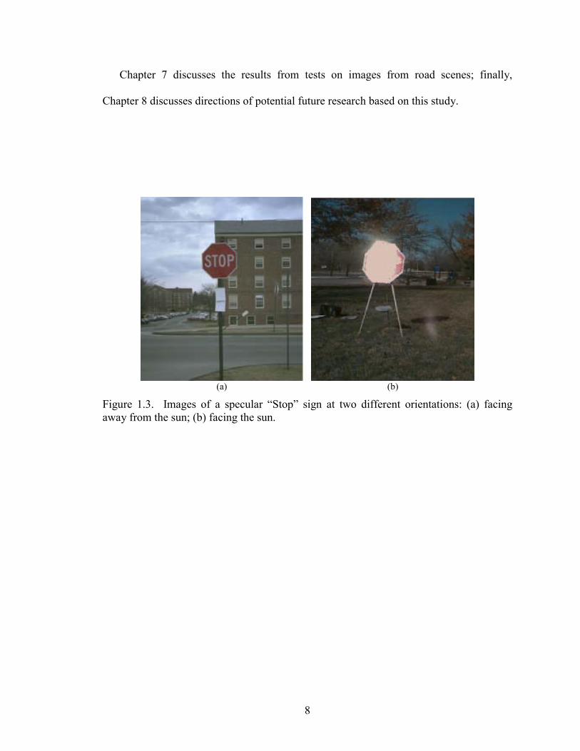
While Figure 1.1 and Figure 1.2 show the variation in the apparent color of simple

matte surfaces, Figure 1.3 and Figure 1.4 show the variation for a specular surface—a

“Stop” sign—from 50 images over the same range of illumination and viewing conditions

as before.4 Figure 1.3 shows “Stop” signs at two different orientations: (a) one facing

away from the sun, and (b) the other, facing the sun (i.e., with the surface normal in the

azimuthal direction of the sun, and partially reflecting the sun into the camera). Figure

1.4 shows the variation in (a) RGB and (b) rgb, respectively, as the orientation and

illuminating conditions change. As the figures demonstrate, the variation in apparent

color of a specular surface can form a bi-modal distribution. In this case, the Cartesian

4 Note that the traffic signs used in this study are privately owned, and do not have retroreflective or fluorescent properties that are required for some public signs. Appendix A contains a more detailed description of these two phenomena.

6

distance between the centroids of the two clusters is about 195 units in RGB and about

0.23 units in rgb. In addition, as Figure 1.4(b) shows, a specular surface may be non-

uniformly colored in an image when direct sunlight is incident upon it. Hence, a portion

of the “Stop” sign is the characteristic red, while another portion exhibits the specular

effect.5

Human beings are able to adapt to this evidently significant color shift due to a

mechanism called color constancy, which is a combination of biological and

psychological mechanisms. Although much work has been done on the processes

involved in human color constancy [2][6][7][34][45][86], it has proven difficult to

successfully simulate the proposed models in computational systems. The

aforementioned examples suggest that in machine vision images, the notion of a color

associated with an object is precise only within the context of scene conditions. The

discussion in Chapter 6 shows that models of daylight color and surface reflectance,

combined with a small number of reasonable assumptions, is an effective way of

modeling scene context.

The discussion in the following chapter shows that color images of outdoor scenes are

complicated by phenomena that are either poorly modeled or described by models which

will more parameters to an already complicated problem. As a result, computational

color recognition has been a difficult and largely unsolved problem in unconstrained

outdoor images. To that end, the two models developed in this study—the daylight and

reflectance models—are shown to be effective in relatively uncontrolled outdoor

environments.

5 Note that the characteristic specular effect of specular surfaces is apparent only when the surfaces are large enough to reflect a portion of direct light onto the camera.

7

Please note that while color prediction is an ideal application to test the two models, it

is not the sole reason for their development; rather, the models attempt to add new insight

into two important processes in outdoor color machine vision (namely, illumination and

reflectance). The color prediction experiments discussed in Chapter 6 require input on

some subset of the following parameters of scene context: sun angle, cloud cover,

illumination angle, viewing angle and sun visibility.

1.3 Overview of chapters

Chapter 2 examines various factors that affect outdoor color images. Chapter 3

examines relevant existing work in color machine vision and shows that existing methods

make assumptions that are not appropriate for unconstrained outdoor images.

In Chapter 4 it is shown that the existing standard model of daylight (the CIE model

[42]) has limitations when applied to machine vision images due to the effect of ambient

light and ground reflection. Hence a model of daylight is built, such that the color of the

incident daylight can be predicted, given the sun-angle and sky conditions.

Chapter 5 shows that the prevalent surface reflectance models [56][70][80] cannot be

easily applied to outdoor images because of their use of brightness values and their

assumptions about the illumination and the independence of the specular effect from

illumination; the Normalized Photometric Function (NPF) is then developed by

simplifying the existing physics-based models for use in outdoor images.

Chapter 6 combines the daylight and NPF models in order to estimate the apparent

color of a target surface under a given set of conditions, and then to classify image pixels

as target or background.

8

Chapter 7 discusses the results from tests on images from road scenes; finally,

Chapter 8 discusses directions of potential future research based on this study.

(a) (b)

Figure 1.3. Images of a specular “Stop” sign at two different orientations: (a) facing away from the sun; (b) facing the sun.

9

(a) Variation in RGB

0

0.2

0.4

0.6

0.8

1

0 0.2 0.4 0.6 0.8 1

g

r

"Stop" sign

(b) Variation in rgb

Figure 1.4. Variation in the apparent color of a specular “Stop” sign over 50 images in: (a) the RGB space; (b) rgb.

10

2 FACTORS IN OUTDOOR COLOR IMAGES

CHAPTER 2

FACTORS IN OUTDOOR COLOR IMAGES

2.1 Overview

Since one major motivation of the models developed in the study is to predict the

apparent color of surfaces in outdoor images, this chapter discusses the significant

processes involved: (a) the color of the incident daylight, (b) surface reflectance

properties, (c) illumination geometry (orientation of the surface with respect to the

illuminant), (d) viewing geometry (orientation of the surface with respect to the camera),

(e) response characteristics of the camera (and peripheral digitization hardware),

(f) shadows, and (g) inter-reflections. In typical outdoor images, some of these factors

remain constant, while others vary. Those that do vary can cause a significant shift in

apparent surface color. The following sections provide some background on the

processes involved in color and image formation, and examine the factors causing the

variation in apparent surface color.

2.2 Light, the visual spectrum, and color

Visible light is electromagnetic energy between the wavelengths of about 380nm and

700nm. Figure 2.1 shows the visible spectrum along with the colors represented by the

various wavelengths.

11

Ultraviolet 400nm 500nm 600nm 700nm Infrared

Figure 2.1. The visible electromagnetic spectrum, approximately between 380nm and 700nm. Just below and above the limits are the ultraviolet and infrared wavelengths, respectively.

Light can be represented by a Spectral Power Distribution (SPD) in the visual

spectrum, which plots the energy at each wavelength (usually sampled at discrete

intervals) between 380nm and 700nm. Figure 2.2 shows simplified SPD's that represent

colors that are shades of pure (a) “red”, (b) “green”, (c) “blue”, and (d) “white”.6 In this

example, the red, green and blue SPD's peak at about 670nm, 550nm and 450nm,

respectively. The white SPD, on the other hand, is flat, since white (by definition)

contains an equal proportion of all colors.7

The SPD's shown in Figure 2.2 are simplified; only very spectrally concentrated light

sources will have such SPD's. The SPD representing the color of daylight is not as

narrow or smooth, as shown in Figure 2.3, which represents a typical blue cloudless sky

[48][94].

6 The names of the colors are in quotes because these are perceptual associations rather than precise definitions. 7 The vertical axis for SPD's denotes the energy radiated; often, the energy measurements at the various wavelengths are normalized [94] and represented relative to a given wavelength. Hence, there is no unit of measurement along the vertical axis.

12

400 500 600 700

Ene

rgy

Wavelength

0

1

400 500 600 700

Ene

rgy

Wavelength

0

1

(a) (b)

400 500 600 700

Ene

rgy

Wavelength

0

1

400 500 600 700

Ene

rgy

Wavelength

0

1

(c) (d)

Figure 2.2. Simplified Spectral Power Distributions (SPD’s) for (a) red, (b) green, (c) blue, and (d) white. The SPD's for the first three colors have peaks at different wavelengths, whereas the white SPD is flat.

400 500 600 700

Ene

rgy

Wavelength

0

1

Figure 2.3. Sample spectral power distribution for daylight from a blue cloudless sky.

13

2.3 The effect of illumination

When light is incident upon a surface, the surface's albedo determines how much of

the incident energy along each wavelength is reflected off the surface, and how much is

absorbed. The resultant reflection, which is the product of the SPD of the incident light

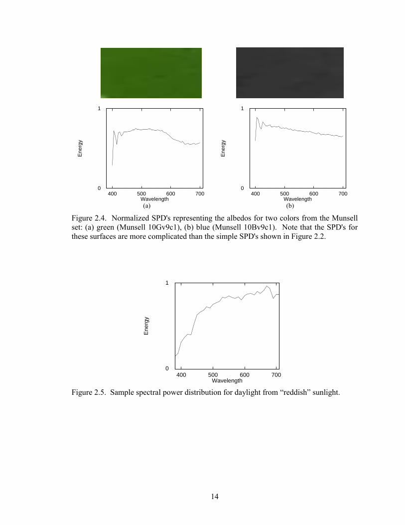
and the albedo, is also represented by an SPD. Figure 2.4 shows the albedo for two

surfaces, blue and green, which are from the Munsell8 color set (numbers 10Bv9c1, and

10Gv9c1, respectively) [48][55].

When white light is incident upon a surface, the SPD of the resultant reflection is the

same as the albedo. However, if the incident light is colored (for instance, red), the

resultant SPD is different from the albedo. If the incident light is a different color (blue,

for instance), the resultant SPD can be significantly different from that under red light. In

outdoor images, the color of the incident daylight is seldom white9 and certainly not

constant; it varies significantly, depending on the sun-angle, cloud cover, humidity, haze

and atmospheric particulate matter [36][42]. Figure 2.5 shows the SPD for the color of

daylight from “reddish” sunlight (at a low sun-angle) [66]; the SPD for this phase of

daylight is quite different from the one shown in Figure 2.3.

Figure 2.6 and Figure 2.7 show the SPD's of the two surfaces from Figure 2.4 under

the two phases of daylight described in Figure 2.3 and Figure 2.5. As the SPD's indicate,

the reflections off the surfaces under different illuminating conditions are significantly

different.

8 The Munsell color chart is a standard set of colors that is often used by color scientists. 9 The color of daylight is closest to white when the whole sky is covered by white clouds; even then, it can have a non-trivial blue component.

14

400 500 600 700

Ene

rgy

Wavelength

0

1

400 500 600 700

Ene

rgy

Wavelength

0

1

(a) (b)

Figure 2.4. Normalized SPD's representing the albedos for two colors from the Munsell set: (a) green (Munsell 10Gv9c1), (b) blue (Munsell 10Bv9c1). Note that the SPD's for these surfaces are more complicated than the simple SPD's shown in Figure 2.2.

400 500 600 700

Ene

rgy

Wavelength

0

1

Figure 2.5. Sample spectral power distribution for daylight from “reddish” sunlight.

15

400 500 600 700

Ene

rgy

Wavelength

0

1

(a) Color patch (b) Original SPD

400 500 600 700

Ene

rgy

Wavelength

0

1

400 500 600 700

Ene

rgy

Wavelength

0

1

(c) SPD under blue sky (d) SPD under red sun Figure 2.6. The Munsell green (number 10Gv9c1) patch (a), with the SPD representing its albedo (b). The SPD of the apparent color of the patch changes (c and d) as the illuminant changes from blue sky to red sun.

The variation in the color of daylight is caused by changes in the sun-angle, cloud

cover, and other weather conditions. In addition, the presence of haze, dust and other

particulate pollutants can also affect the color of daylight in localized areas [36]. The

CIE model [42] has served as the standard for the variation of the color of daylight, and

has empirically been shown to be accurate in radiometric data. However, as Chapter 4

shows, the model has three disadvantages when applied to machine vision images,

namely that it does not account for the effect of ambient light or ground reflection, and

16

there is very little context-specific data mapping illumination conditions to incident light

color. Hence, Chapter 4 develops a model specifically for machine vision. Note that one

additional consequence of the variation in the color of daylight is illuminant metamerism,

where two surfaces with different albedos and under different illuminant colors, map to

the same apparent color. Although this is a rare phenomenon, it cannot be avoided and is

one of the causes of errors in applications of the techniques developed in this study.

400 500 600 700

Ene

rgy

Wavelength

0

1

(a) Color patch (b) Original SPD

400 500 600 700

Ene

rgy

Wavelength

0

1

400 500 600 700

Ene

rgy

Wavelength

0

1

(c) SPD under blue sky (d) SPD under red sun Figure 2.7. The Munsell blue (number 10Bv9c1) patch (a) with the SPD representing its albedo (b), and the SPD's under (a) blue sky, and (d) red sun.

17

2.4 The effect of surface orientation and reflectance

Illumination geometry, i.e., the orientation of the surface with respect to the sun,

affects the composition of the light incident upon the surface. Daylight has two

components, sunlight and ambient skylight, and the surface orientation determines how

much light from each source is incident on the surface. For instance, a surface that faces

the sun is illuminated mostly by sunlight, whereas one that faces away is illuminated

entirely by the ambient skylight and light reflected off other surfaces in the scene. The

reflectance properties of the surface determine the combined effect of illumination

geometry and viewing geometry (i.e., its relative viewing geometry). Figure 2.8 explains

some of the terminology related to surface orientation. The strength of the specular

reflectance component of the surface, based on the combined geometry of illumination

and viewing, affects the composition and amount of light reflected by the surface onto the

camera (as shown earlier in Figure 1.3 and Figure 1.4). While physics-based reflectance

models exist [46][56][70][80], they cannot be easily used with outdoor images because

(i) they assume single-source illumination, (ii) they do not account for the effect of

illuminant obscuration on the specular effect, and (iii) they rely on illuminant brightness,

which cannot be easily estimated for daylight (shown in Chapter 5). Hence, Chapter 5

develops the Normalized Photometric Function, which can be applied to outdoor data and

to the daylight model developed earlier in the same chapter.

18

Figure 2.8. The geometry of illumination and viewing depends on the position of the illuminant and camera (respectively) with respect to the surface. Along the surface normal, the angle is 0°, and ranges from 90° to 90° on either side of the surface normal. The relative viewing geometry is the combination of the illumination and viewing geometries.

2.5 The effect of the sensor

Before a discussion of the effect of sensor (camera) characteristics, the following

description of color spaces may be helpful. A color digital image represents scenes as

two-dimensional arrays of pixels. Each pixel is a reduced representation of an SPD,

where the reduction depends on the color space being used. One commonly used space is

the three-dimensional RGB (Red-Green-Blue) space, which is derived from a set of

(three) trichromatic filters [94]. While there are canonical “RGB” spaces, manufacturing

inaccuracies cause each camera to, in effect, have its own unique RGB space. Hence,

each camera should be calibrated to determine its unique response parameters; the

calibration parameters for the camera used in this study are shown in Table 2.1. Figure

2.9(a) shows the spectral transmission curves for a set of three filters10 used to derive a

hypothetical RGB. For each pixel, the product of each of the trichromatic filters and the

input SPD is integrated, and the resulting sum then becomes the value of the pixel along

10 The filters shown in Figure 2.9 are the CIE color matching functions [94]. The RGB color space(s) used by most cameras are linear transforms of these functions [37].

19

the corresponding dimension. The RGB space represents the brightness (intensity) of a

pixel along each dimension, ranging (usually) from 0 to 255. In such a framework, the

color “black” is represented by the value [0,0,0], “white” by [255,255,255], a pure bright

“red” by [255,0,0], “green” by [0,255,0], and “blue” by [0,0,255] (once again, the colors'

names are in quotes because these are qualitative and perceptual associations rather than

precise quantitative definitions.). One of the consequences of reducing the representation

of color from the continuous SPD function to a three-dimensional value is that a number

of physically different SPD's can be mapped to the same RGB value. This phenomenon

is known as observer metamerism, and even humans perceive metamers as being similar;

fortunately, this type of metamerism is not a common occurrence in practice.

The RGB space can be normalized over total brightness, such that r=R/(R+G+B),

g=G/(R+G+B), and b=B/(R+G+B). The normalized space, referred to hereafter as rgb,

eliminates the effect of brightness, and the value along each of the dimensions (in the

range 0-1) represents the pure color without brightness. Hence, black, white, and all the

grays in between are mapped to the same value [0.33,0.33,0.33]. In rgb, r+g+b = 1;

given the values along only two of the dimensions, the third can be determined.

Therefore, rgb is a two-dimensional space.

20

400 450 500 550 600 650 700 (a) Trichromatic filters

(b) RGB space

Figure 2.9. Trichromatic filters (a) used to reduce an SPD to the RGB color space (b). Of the three filters, the “red” filter peaks at about 440nm, “green” at about 550nm, and the “blue” filter has a large peak at about 600nm and a smaller one at about 440nm.

Factor Model Comments

Focal length 6.5mm (equivalent to 37mm on a 35mm camera)

Color filters Based on NTSC RGB standard primaries [76]

Calibration required

White point [0.326, 0.341, 0.333] Obtained with a calibrated white surface (Munsell N9/) under D65 illuminant

Gamma correction γ = 0.45 f-stop adjusted to stay in the 50-75%, (approximately linear) output range

Aperture range f/2.8 to f/16 Aperture adjusted with f-stop

Shutter speed 1/30 to 1/175 seconds

Image resolution 756×504, 24-bit RGB

Gain 2.0 e-/count Fixed

Table 2.1. Parameters of the camera used in this study.

21

The response characteristics typical to digital cameras (or other imaging devices used

for machine vision) can cause apparent surface color to shift in a number of ways. In the

process of reducing the SPD's at individual pixels to RGB digital values, a number of

other approximations and adjustments are made, some of which have a significant impact

on the resultant pixel colors, while others have a relatively small effect. To begin with,

wavelength-dependent displacement of light rays by the camera lens onto the image plane

due to chromatic aberration can cause color mixing and blurring [5]. However,

experiments in the literature [5] suggest that the effects of chromatic aberration will have

a significant impact only on those methods that depend on a very fine level of detail.

Observer metamerism, introduced in the previous section, occurs when different SPD's

are mapped to the same RGB value [92]. Although this process does not shift or skew the

apparent color of an object, it can cause ambiguity since two physically distinct colors

(with respect to their respective SPD's) can have the same RGB value; in practice, as

mentioned before, this does not occur very often. Many cameras perform pixel-level

color interpolation on their CCD (Charge-Coupled Device) arrays, which convert the

incident light energy at every pixel (photo-cell) to an electrical signal. On the photo-

receptor array, each pixel contains only one of the three RGB filters, and the other two

values are calculated from neighboring pixels at a later stage. Figure 2.10(a) shows the

color filter array in the Kodak DC-40 digital camera. After the reduction of the SPD's to

three separate electrical signals, the digitizer converts each input electrical signal to a

digital value. Many digitizers use a nonlinear response function because the output of the

camera is assumed to be a monitor or other display device (the phosphors for which are

inherently nonlinear). The nonlinear response of the digitizer is meant to compensate for

22

the monitor nonlinearity; while this may help in displaying visually pleasing images, it

can cause a problem for image analysis. The nonlinear response function is determined

by a gamma-“correction” factor (shown in Figure 2.10(b)), which is 0.45 for many

commonly used digital cameras [18]. On many cameras, gamma-correction can be

disabled; on others it is possible to linearize the images through a calibration lookup table

[60]. The dynamic range of brightness in outdoor scenes accentuates the possibility of

clipping (photo-cell/pixel saturation) and blooming (draining of energy from one

saturated photo-cell to a neighboring photo-cell) [60]. Although pixel clipping is easy to

detect, there are no reliable software methods for correcting the problem. Blooming is

difficult to even detect; while fully saturated pixels can easily be detected, the effect on

photo-cells receiving excess energy from neighboring cells is more difficult to detect.

Hence, blooming is not easily detectable or correctible [60].

The images used in this study were collected using a Kodak digital camera

(customized DC-40), the relevant parameters for which are listed in Table 2.1. The

automatic color balance on the camera was disabled, and the f-stop adjusted so that the

output was always in the 50-75% (approximately linear) range; this avoided nonlinear

response and pixel clipping. In addition, a color calibration matrix was obtained based on

standard techniques [76], using a calibrated white surface (Munsell N9/) under a D65

illuminant. However, three other camera-related problems, namely blooming, chromatic

aberration, and the mixed-pixel effect were considered either unavoidable or negligible,

and not addressed specifically.

23

G R

G

G

G

G

G G GR R

B BG G GB B

G G G

G G G

R R R

GB B B BG

R R R

B B B BG G

0

0.25

0.5

0.75

1

0 0.25 0.5 0.75 1

Cam

era

Out

put S

igna

l

Input Light Intensity

Nonlinear response (Gamma correction)

Gamma = 0.45

(a) Pixel interpolation (b) Gamma-correction

Figure 2.10. Sources of color shifts in digital cameras: (a) pixel interpolation, (b) nonlinear response. With pixel interpolation each pixel (photo-cell) has only one color filter, and the other two color values are approximated from neighboring pixels. With gamma-“corrected” nonlinear response, the output signal is adjusted for display purposes according to the rule (o = iγ), where o is the output signal, i is the input light intensity, and γ the correction factor.

2.6 Shadows and inter-reflections

Inter-reflections and shadows can cause a further variation in apparent color by

adding indirect incident light or by restricting the effect of the existing light sources,

thereby altering the color of the light incident upon the surface. Inter-reflections, for

instance, cause light reflected off other surfaces in the scene to be incident upon the

surface being examined. In fact, Chapter 4 shows that the color of daylight departs

significantly from the CIE daylight model, due in part to light reflected off the ground.

Beyond that, however, the effect of inter-reflections in complicated scenes can be hard to

estimate [31]. Therefore, in this study, it is assumed that the scenes do not contain large,

brightly colored objects near the target surface.

Shadowing can be of two types: self-shadowing and shadowing by another object.

Chapter 4 shows that when the object is self-shadowed, the final effect is that the surface

is illuminated both by skylight and by indirect sunlight reflected off the ground; this

24

effect is taken into account while determining the color of the incident light. On the other

hand, if a surface is shadowed by a secondary object, the effects depend on the secondary

object, and can cause all the effects of self-shadowing and additional inter-reflection off

the secondary object. In this study, since it is assumed that there is no significant inter-

reflection (other than off the ground), it is assumed that the effect of secondary

shadowing is no different from that of self-shadowing.

Table 2.2 summarizes the various factors that contribute to the variation of apparent

color in outdoor images, along with relevant models for those factors and the problems (if

any) with those models. Note that many of these factors apply to indoor images as well.

The above discussion indicates that color images of outdoor scenes are complicated

by phenomena that are either poorly modeled or inadequately described by models which

add more parameters to an already complicated problem. As a result, problems such as

apparent color prediction have been difficult and largely unsolved in unconstrained

outdoor images. To that end, the contributions of this work include useful context-based

models of daylight and reflectance that can be applied when either full or partial

contextual information is available.

25

Factor Models Problems Solutions Daylight: Sun-angle & sky conditions

CIE [42] • Little or no context-based information

• Does not account for ambient or stray/indirect light

• Context-based model developed

• Model accounts for moderate amounts of stray and incident light

Daylight: Haze, pollution

None Difficult to model [36] Ignored

Reflectance: Surface orientation (w.r.t., illuminant and camera)

Lambertian [38]; Dichromatic [80]; Hybrid [56]; Shading [70]

• Assumptions about single-source illuminant

• Use of brightness values • Specular effect does not

account for illuminant obscuration

• Models adapted for extended 2-source illuminant (daylight)

• Brightness issues eliminated by normalization

• Reflectance model explicitly accounts for illuminant obscuration

Camera: Nonlinear response

Supplied with camera

Nonlinear only near extremes of sensor range

f-stop adjusted: only middle, approximately linear range used

Camera: Chromatic aberration

Boult [5] Affects mostly edge pixels Ignored

Camera: Clipping Novak [60] Can be detected but not corrected

Pixels detected and eliminated

Camera: Blooming Novak [60] Cannot be easily detected or corrected

Ignored

Shadows None [31] Difficult to model • Self-shadowing modeled as incident ambient light

• Direct shadowing ignored

Inter-reflections None [31] Difficult to model • Ground reflection modeled in daylight model

• Other inter-reflections ignored

Table 2.2. Factors affecting the apparent color of objects in outdoor images, existing models and problems (if any) with those models, as well as ways in which this study addresses the problems.

26

3 PREVIOUS WORK CHAPTER 3

PREVIOUS WORK

3.1 Overview

This chapter discusses prevalent work in three areas: color prediction/recognition

techniques (e.g., color constancy) in Section 3.2, models of daylight in Section 3.3, and

surface reflectance models in Section 3.4. As Section 3.2 shows, research in color

machine vision has a rich history; however, there has been little work exploring issues in

outdoor images. The primarily physics-based models in Sections 3.3 and 3.4 that are

related to the issues in this work make strong assumptions that may not hold in outdoor

images.

3.2 Color machine vision

Research in color machine vision has a rich history, although relatively little of it

explores issues in outdoor images. Existing work in relevant aspects of color vision can

be divided into two categories: computational color constancy and physics-based

modeling. In addition, there is a body of research related to color vision in the areas of

parametric classification [16], machine learning techniques [10], color-based

segmentation [51][64][79], application-driven approaches [16][73], and color indexing

[28][82][85]. Finally, a number of other studies have been developed for particular

applications or domains [12][13][41][54][67][71][84][88][91][96], but do not deal with

issues related to outdoor color images.

27

3.2.1 Color constancy

Most of the work in computer vision related to the variation of apparent color has

been in the area of color constancy, where the goal is to match object colors under

varying, unknown illumination without knowing the surface reflectance function. An

illuminant-invariant measure of surface reflectance is recovered by first determining the

properties of the illuminant.

Depending on their assumptions and techniques, color constancy algorithms can be

classified into six categories [26]: (1) those which make assumptions about the statistical

distribution of surface colors in the scene, (2) those which make assumptions about the

reflection and illumination spectral basis functions, (3) those that assume a limited range

of illuminant colors or surface reflectances, (4) those which obtain an indirect measure of

the illuminant, (5) those which require multiple illuminants, and (6) those which require

the presence of surfaces of known reflectance in the scene. Among the algorithms that

make assumptions about statistical distributions, von Kries and Buchsbaum assume that

the average surface reflectance over the entire scene is gray (the gray-world assumption)

[8][44]; Gershon [31] assumes that the average scene reflectance matches that of some

other known color; Vrhel [89] assumes knowledge of the general covariance structure of

the illuminant, given a small set of illuminants; and Freeman [25] assumes that the

illumination and reflection follow known probability distributions. These methods are

effective when their assumptions are valid. Unfortunately, as the examples in Chapter 1

(Figure 1.1, Figure 1.2, Figure 1.3, Figure 1.4) show, no general assumptions can be

made about the distribution of surface colors without knowledge of the reflectance, even

28

if the distribution of daylight color is known. Consequently, these methods are too

restrictive for all but very constrained scenes.

The second category of color constancy algorithms make assumptions about the

dimensionality of spectral basis functions [81] required to accurately model illumination

and surface reflectance. For instance, Maloney [49] and Yuille [95] assume that the linear

combination of two basis functions is sufficient. It is not clear how such assumptions

about the dimensionality of spectral basis functions in wavelength space apply to a

reduced-dimension color space, such as the tristimulus RGB (Finlayson [22] discusses

this issue in greater detail).

Among the algorithms that assume limits on the potential set of reflectances and

colors in images is Forsyth's CRULE (coefficient rule) algorithm [24], which maps the

gamut (continuum) of possible image colors to another gamut of colors that is known

a priori, so that the number of possible mappings restricts the set of possible illuminants.

In a variation of the CRULE algorithm, Finlayson [20] applies a spectral sharpening

transform to the sensory data in order to relax the gamut constraints. This method can be

applied to algorithms using linear basis functions [49][95] as well. CRULE represents a

significant advance in color constancy, but its assumptions about gamut mapping restrict

it to matte Mondrian surfaces or controlled illumination; this is largely because

uncontrolled conditions (or even specularity) can result in the reflected color being

outside the limits of the gamut map defined for each surface without the help of a model

of daylight. Ohta [63] assumes a known gamut of illuminants (indoor lighting following

the CIE model), and uses multi-image correspondence to determine the specific

29

illuminant from the known set. By restricting the illumination, this method can only be

applied to synthetic or highly constrained indoor images.

Another class of algorithms uses indirect measures of illumination. For instance,

Shafer [80] and Klinker [43] use surface specularities (Sato [77] uses a similar principle,

but not for color constancy), and Funt [27] uses inter-reflections to measure the

illuminant. These methods assume a single point-source illuminant, which limits their

application in outdoor contexts, since daylight is a composite, extended light source.

In yet another approach, D'Zmura [97] and Finlayson [21] assume multiple

illuminants incident upon multiple instances of a single surface. The problem with these

approaches is that they require identification of the same surface in two different parts of

the image (i.e., multiple instances of a given set of surface characteristics) that are subject

to different illuminants. Once again, the approaches have been shown to be effective

only on Mondrian or similarly restricted images. In a variation of this approach,

Finlayson [23] shows good results on a set of synthetic and real images by correlating

image colors with the colors that can occur under each set of possible illuminants.

The final group of algorithms assume the presence of surfaces of known reflectance

in the scene and then determine the illuminant. For instance, Land's Retinex algorithm

[45] and its many variations rely, for accurate estimation, on the presence of a surface of

maximal (white) reflectance within the scene. Similarly, Novak's supervised color

constancy algorithm [61] requires surfaces of other known reflectances.

Funt [26][29] discusses the various approaches to color constancy in greater detail.

The assumptions made by the aforementioned algorithms limit their application to

restricted images under constrained lighting; certainly, few such methods have been

30

applied to relatively unconstrained outdoor images. It therefore makes sense to develop

models for outdoor illumination and surface reflectance under outdoor conditions.

3.2.2 Parametric classification

The emergence of road-following as a machine vision application has spawned

several methods for utilizing color to enable autonomous vehicles drive without specific

parametric models. Crisman's SCARF road-following algorithm [16] approximates an

“average” road color from samples, models the variation of the color of the road under

daylight as a Gaussian distribution about an “average” road color, and classifies pixels

based on minimum-distance likelihood. This technique was successfully applied to road-

following, but cannot be applied for general color recognition, because the variation of

the color of daylight according to the CIE model [42] cannot be modeled as Gaussian

noise. At the same time, the notion of an “average” color for the entire gamut under

changes of illumination and scene geometry may not be constrained enough for

classifying pixels under specific conditions. One of the contributions of this dissertation

is a definition of underlying models of illumination and reflectance, so that apparent

object color under specific conditions can be localized to a point in color space with an

associated Gaussian noise model for maximum-likelihood classification.

3.2.3 Techniques based on machine-learning

Pomerleau's ALVINN road-follower [73] uses color images of road scenes along with

user-generated steering signals to train a neural network to follow road/lane markers.

However, the ALVINN algorithm made no attempt to explicitly recognize the apparent

color of lanes or roads, or to model reflectance.

31

Buluswar [10] demonstrates the use of machine-learning techniques for non-

parametric pixel classification as an approach to color “recognition”. Multivariate

decision trees and neural networks are trained on samples of target and non-target

“background” surfaces to estimate distributions in color space that represent the different

apparent colors of the target surface under varying conditions; thereafter, image pixels

are classified as target and background. This approach was shown to be very effective

for color pixel classification in several outdoor applications. The problem with such non-

parametric techniques is that their performance is determined entirely by the training

data: if there is training data for the set of encountered illumination and viewing

conditions and for non-target surfaces that can be expected in the images, then such

techniques can approximate discriminant boundaries around them. In the absence of such

data, however, the performance of non-parametric classification techniques in the

“untrained” portions of color space is unpredictable. Funt [30] also approaches color

constancy as a machine learning problem; as with other learning-based approaches, a

potential issue with this technique is that the training data needs to represent the gamut of

possible conditions that can occur, without which it is difficult to expect accurate

performance.

3.2.4 Color segmentation

In the problem of segmentation, the goal is to separate spatial regions of an image on

the basis of similarity within each region and distinction between different regions.

Approaches to color-based segmentation range from empirical evaluation of various color

spaces [64], to clustering in feature space [79], to physics-based modeling [51]. The

essential difference between color segmentation and color recognition is that the former

32

uses color to separate objects without a priori knowledge about specific surfaces, while

the latter attempts to recognize colors of known color characteristics. Although the two

problems are, in some sense, the inverse of each other, results from segmentation can be

useful in recognition; for instance, Maxwell [51] shows the advantages of using

normalized color and separating color from brightness.

3.2.5 Color indexing

Swain [82] introduced the concept of color histograms for indexing objects in image

databases, proving that color can be exploited as a useful feature for rapid detection.

Unfortunately, this method does not address the issue of varying illumination, and hence

cannot be applied to general color recognition in outdoor scenes. Funt [28] uses ratios of

colors from neighboring locations, so as to extend Swain's method to be insensitive to

illumination changes; unfortunately this method requires histograms of all the objects in

the whole scene to vary proportionally.

3.3 Models of daylight

As Chapter 4 discussed, the CIE model [42] has been used to define the color of a few

specific phases of daylight, and to parametrically model the overall variation of daylight

color. This radiometric model has been confirmed by a number of other radiometric

studies in various parts of the world [19][35][58][66], and has been used by several

machine vision researchers [21][63] in digital images. Chapter 4 shows—in detail—that

the CIE radiometric model cannot be applied to machine vision images because it does

not account for (i) ambient light from a sufficiently large portion of the sky, and (ii) the

effect of light reflected off the ground. In addition, the lack of context-specific data

33

makes the CIE model difficult to use in a wide range of conditions where the specific

color of the incident light is required.

While the CIE model has been the most widely applied model in the context of color

images, Sato [77] develops an intensity-based model in which sunlight is characterized as

a “narrow Gaussian distribution” [77]. However, the model requires bright sunlight

without any clouds, and does not account for the effect of a cloud cover or sun-

obscuration (partial or full). Hence the applicability of Sato's model for color images

with unconstrained sky conditions is unclear.

3.4 Surface reflectance models

In general, surface reflectance can be modeled by a bidirectional reflection

distribution function (BRDF) [17][38][59], which describes how light from a given

direction is reflected from a surface at a given orientation. Depending on the

composition of the incident light and the characteristics of the surface, different spectra of

light may be reflected at different orientations, thereby making the BRDF very complex.

The simplest model of reflectance is the Lambertian model [38], which predicts that

light incident upon a surface is scattered equally in all directions, such that the total

amount of light reflected is a function of the angle of incidence. The Lambertian

model—and modifications thereof [65][93]—are used to describe reflectances of matte

surfaces.

However, for modeling surfaces which have a specular component, a number of

researchers use a composite of the specular and Lambertian components

[15][43][46][56][77][80][87][97]. For instance, Shafer [80] models surface reflectance

as a linear combination of the diffuse and specular components, and determines the

34

weights of each component from a measure of specularity. Shafer's Dichromatic

Reflectance Model shows that color variation in RGB lies within a parallelogram, the

length and breadth of which are determined by the two reflectance components. Klinker

[43] refines the Dichromatic model by showing that surface reflectance follows a “dog-

legged” (“┴”-shaped) distribution in RGB, and then fits a convex polygon to separate the

reflectance components. In a variation of Shafer's approach, Sato [78] uses temporally

separated images to model the surface components. Each of these methods depends on

the presence of pure specular reflection from a point-source light. As Chapter 4 will

show, daylight is a composite, extended light source, not a point-source; consequently,

none of the aforementioned approaches have been applied to outdoor images. Lee [46]

derives the Neutral Interface Reflectance model which also models surface reflectance as

a linear combination of the two reflectance components and demonstrates the

effectiveness of his model on spectral power distributions of surfaces. Unfortunately,

Lee stops short of applying his methods to real digital images. Sato [77] applies the

Neutral Interface model and approximates sunlight as a “narrow” Gaussian (with a low

standard deviation) to recover the shape of surfaces in outdoor digital images. In another

approach to determining shape from shading, Nayar [56] uses photometric sampling (a

method of sampling reflectance under varying viewing geometry) to model surface

reflectance. While the methods developed by Nayar and Sato have been used for shape-

extraction, neither has been used to model reflectance in color space. None of the

aforementioned models have been used in the context of estimating apparent color in

outdoor images; some of the above bear particular relevance to the Normalized

35

Photometric Function model developed in Chapter 5, and will be analyzed in greater

detail there.

As the preceding discussion indicates, there is almost no work that attempts to

estimate apparent color in realistic outdoor images (the one exception, Buluswar [10],

classifies pixels without explicitly modeling or estimating apparent surface color). The

goal of this dissertation is to adapt (and simplify) existing physics-based models and

thereby develop a method applicable to outdoor images.

36

4 A MODEL OF OUTDOOR COLOR CHAPTER 4

A MODEL OF OUTDOOR COLOR

4.1 Overview

The first major contribution of this work is a detailed discussion of daylight color.

Even though a standard model for the variation of daylight color (the CIE model [42])

exists, this section shows that the CIE model has three disadvantages that reduce its

applicability to machine vision. First, the CIE radiometric equipment has a very small

field-of-view (e.g., 0.5o and 1.5o [66]), in order to sample a small portion of the sky. On

the other hand, when daylight is incident upon a surface, the FOV of the surface can be

up to 180o, which means that there can be a significant amount of incident ambient light;

the CIE model does not account for this ambient light. Secondly, in typical machine

vision images, a significant amount of light is reflected off the ground, thus changing the

composition of the light incident upon surfaces close to the ground; the CIE model does

not account for such indirect light. Finally, there is very little context-specific information

in the CIE model [14], which means that it is difficult to use the model to predict the

color of daylight under specific conditions. As a consequence of these three issues, the

CIE model cannot be used to estimate the apparent color of a surface, even if the

illuminating conditions are specified. In order to deal with these problems, Section 4.4

develops a context-based model of daylight color that makes it possible to predict the

color of the incident light under specific conditions (sun angle and cloud cover); this

prediction is then combined with a reflectance model developed in Chapter 5.

37

4.2 The CIE daylight model

The CIE daylight model [42] is based on 622 radiometric measurements of daylight

collected separately over several months in the U.S.A., Canada, and England [9][14][35].

Such radiometric measurements are typically made by aiming a narrow tube [14] with a

very small field-of-view (e.g., 0.5o and 1.5o [66]) at a selected portion of the sky. The

light going through the collection tube falls on a planar surface covered with barium

sulphate (or a similar “white” material), and the spectral power distribution of the surface

is recorded. In the CIE studies, careful precautions were taken so as to eliminate the

effect of stray light—for instance, the data was collected on roof-tops, and all nearby

walls and floors, and even the collection tube, were covered by black light-absorbent

material [14].

The parametric model was then obtained by mapping the spectral power distributions

of each of the 622 samples into the CIE chromaticity space, and then fitting the following

parabola to the points:

y = 2.8x – 3.0x2 – 0.275 (4.1)

where 0.25 ≤ x ≤ 0.38. In the rgb space (which is a linear transform of the chromaticity

space [37]), the model is:

g = 0.866r – 0.831r2 + 0.134 (4.2)

where 0.19 ≤ r ≤ 0.51. Figure 4.1 plots the daylight model in rgb; the figure also plots

the CIE daylight model in the color circle. The regions of the function representing

(approximately) sunlight and skylight (Figure 4.1(b)) have been determined empirically,

based on radiometric measurements made by Condit [14] and the measurements shown in

Table 4.1 (which is discussed later in this section).

38

For mathematical simplicity, the experiments that follow in later sections will

approximate the CIE parabola by the following straight line, also shown in Figure 4.1(c):

g = 0.227 + 0.284 r (4.3) which was determined by fitting a line to discrete points along the locus of the CIE

parabola in rgb. The RMS error introduced by the linear approximation (determined by

point-wise squared error for g-values generated for discrete r-values in the range 0.19 ≤ r

≤ 0.51 at increments of 0.005) is 0.007. Figure 4.1(c) compares the linear and quadratic

models.

4.3 Daylight in machine vision images

The goal of the CIE studies was to obtain the precise color of daylight under some

specific conditions (e.g., noon in a clear sky, etc.). One of the motivations behind the

studies appears to be the design of artificial light sources [42]. Hence, some canonical

illumination conditions (such as noon sunlight and “average” daylight [42] were used as

models for artificial light sources. In order to assure the accuracy of the measurements,

high-precision radiometric equipment was used, and precautions were taken to prevent

stray light from entering the experimental apparatus. In addition, only small portions of

the sky were sampled by using the narrow collection tube.

Although these restrictions were required for the purposes of the radiometric studies,

such conditions are not typical in outdoor computer vision images. As explained in

Chapter 2, machine vision images are subject to a number of factors that can cause shifts

in the color of the incident light. We collected samples of daylight under varying

conditions from 224 color images of a calibrated matte white surface (Munsell number

N9/), where the apparent color of the white surface is the color of the light incident upon

39

it. Figure 4.2 shows the sampling apparatus, along with samples of the color of daylight

obtained from the set of 224 images, plotted in rgb. The exact set of illumination

conditions sampled in these images is described in Table 4.1.

Figure 4.2(a) shows a board with a number of matte surfaces of different colors,

mounted on a tripod which has angular markings at every 5o, along with accompanying

adjustments on a rotatable head-mount. The surface in the middle of the board is the

Munsell White, and is used to sample the incident light. During data collection, the

angular markings on the tripod were used to vary the viewing geometry in the azimuth;

images were taken at every 10o. The viewing geometry with respect to pitch was

(approximately) fixed by maintaining a constant distance between the camera and the

surface, as well as a constant camera height. For the measurements at each sampled sun-

angle, the illumination geometry was also fixed with respect to pitch, but varied in the

azimuth using the tripod angular settings. Using this procedure, it was determined that

for almost11 the whole 180o range where the sun is directly shining on the surface, the

color of the incident daylight does not change with respect to varying relative viewing

geometry. Similarly, as long as the surface is facing away from the sun, the color of the

incident light is that of the skylight incident upon the surface. A total of 224 samples of

daylight were collected under the illuminating conditions described in Table 4.1. The

conditions were chosen so as to capture the maximum possible variation in the color of

the light each day. In order to reduce the effect of pixel-level noise, the color of the white

surface was sampled as the average over a 20 pixel × 20 pixel area. Figure 4.2(b) shows

the data collected using the apparatus in Figure 4.2 (a), plotted against the linear

11 At the extreme angles (e.g., near the -90o and 90o viewing angles), too little of the surface is visible for any meaningful analysis.

40

approximation of the CIE model. The root-mean-squared error12 between the linear CIE

model and the observed data was only 0.006. However, the Cartesian spread of our data

was 0.162, about 46% of the spread of the CIE model, which is 0.353. In other words,

our data covers only a portion of the full range of daylight color predicted by the CIE

model, even though both studies sampled a similar range of sky conditions. In order to

determine why the spread in CIE data is more than twice that in our data, the

observations are divided into two groups: (i) those with an r value less than 0.33 (which,

as discussed in Figure 4.1, represent samples of daylight from the direction away from

the sun), and (ii) those with an r value greater than 0.33 (which represent samples from

the direction of the sun).

12 For every r value from the observed data (all of which were within the r range of the CIE model), a g value was calculated using the CIE model in Equation 4.2, and then compared to the corresponding g value in the observed data. Thereafter, the root-mean-squared error between the two sets of g values was calculated.

41

0

0.2

0.4

0.6

0.8

1

0 0.2 0.4 0.6 0.8 1

g

r

SunSky

CIE modelSun vs Sky

(a) rgb

(b) Color circle

0.2

0.3

0.4

0.5

0.1 0.2 0.3 0.4 0.5 0.6

g

r

CIE parabolaLinear approximation

(c) Linear approximation

Figure 4.1. The CIE parametric model of daylight in (a) the rgb space and (b) the color circle. The sunlight and skylight components have been empirically determined to be on either side of the white point ([0.33, 0.33] in rgb and the center of the color circle). The CIE studies [42] describe the factors causing the variation. Figure (c) shows the linear approximation to the CIE parabola that this study uses for mathematical simplicity in later sections.

42

(a) Sampling apparatus

0.2

0.3

0.4

0.5

0.1 0.2 0.3 0.4 0.5 0.6

g

r

Observed dataLinear CIE model

(b) Observed samples vs. CIE model

Figure 4.2. Samples of daylight color obtained from color images, compared to the CIE model. The white surface in the center of image in Figure (a) reflects the color of the incident light. These samples are plotted along with the linear approximation of the CIE model in Figure (b).

43

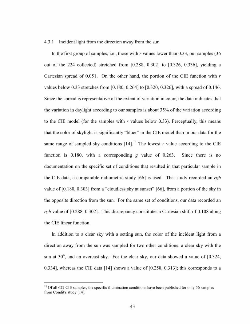
4.3.1 Incident light from the direction away from the sun

In the first group of samples, i.e., those with r values lower than 0.33, our samples (36

out of the 224 collected) stretched from [0.288, 0.302] to [0.326, 0.336], yielding a

Cartesian spread of 0.051. On the other hand, the portion of the CIE function with r

values below 0.33 stretches from [0.180, 0.264] to [0.320, 0.326], with a spread of 0.146.

Since the spread is representative of the extent of variation in color, the data indicates that

the variation in daylight according to our samples is about 35% of the variation according

to the CIE model (for the samples with r values below 0.33). Perceptually, this means

that the color of skylight is significantly “bluer” in the CIE model than in our data for the

same range of sampled sky conditions [14].13 The lowest r value according to the CIE

function is 0.180, with a corresponding g value of 0.263. Since there is no

documentation on the specific set of conditions that resulted in that particular sample in

the CIE data, a comparable radiometric study [66] is used. That study recorded an rgb

value of [0.180, 0.303] from a “cloudless sky at sunset” [66], from a portion of the sky in

the opposite direction from the sun. For the same set of conditions, our data recorded an

rgb value of [0.288, 0.302]. This discrepancy constitutes a Cartesian shift of 0.108 along

the CIE linear function.

In addition to a clear sky with a setting sun, the color of the incident light from a

direction away from the sun was sampled for two other conditions: a clear sky with the

sun at 30o, and an overcast sky. For the clear sky, our data showed a value of [0.324,

0.334], whereas the CIE data [14] shows a value of [0.258, 0.313]; this corresponds to a

13 Of all 622 CIE samples, the specific illumination conditions have been published for only 56 samples from Condit's study [14].

44

Cartesian shift of 0.069 along the CIE linear function. On the other hand, for the overcast

sky, our measure was [0.357, 0.335], very close to the CIE measure of [0.360, 0.336].

(a) Narrow FOV device (b) Wider FOV device (c) Planar surface with 180o FOV

Figure 4.3. Illustrative examples of devices/objects with different fields-of-view: (a) tube-like sensors/devices such as telescopes and photometers have narrow FOV’s; (b) cameras have a wider FOV; (c) planar surfaces, on the other hand, have light incident from the full 180o “field-of-view”. The implication of this phenomenon for outdoor images is that planar surfaces will have light incident upon it from a much larger portion of the sky than will the photo-receptor sensors of photometers (with collection tubes) or cameras.

The following discussion shows that when there is a discrepancy between the CIE

model and our data, two factors account for the shift: (i) ambient skylight from a large

portion of the sky (which is incident upon the surface because of the 180o FOV, and (ii)

sunlight reflected off the ground. It is shown that the effect of ambient skylight accounts

for about 75% of the shift, while the ground's reflection of sunlight accounts for about

20%. In the case of an overcast sky, there is very little variation in the color of the

ambient skylight. At the same time, the sun is not visible, as a consequence of which the

ground does not reflect the color of the sunlight.

5o

45o

180o

45

4.3.1.1 The effect of ambient skylight

Figure 4.3 illustrates the significance of the field-of-view in outdoor images; the

figure shows three objects: (a) a telescope (with dimensions representative of some

photometeric tubes) with a narrow FOV (5o); (b) a camera with a wider FOV (45o), and

(c) a planar surface, which has a 180o FOV. In the context of outdoor illumination,

planar surfaces will have light incident upon it from a much larger portion of the sky.

The field-of-view of the measuring devices used in the CIE radiometric studies was

significantly smaller than that of the planar surfaces used for collecting our data; as a

result, our samples include a greater effect of ambient light. For instance, in the

radiometric study cited above [66], the field-of-view of the sampling device was 0.5o

(horizontal) and 1.5o (vertical); on the other hand, the white sampling surface used in our

apparatus has a field-of-view of practically 180o. The sampling surface is Lambertian,

which means that its apparent color will be affected by light from every source in its

field-of-view. As a consequence, while the radiometric equipment measures the color of

light from a very small portion of the sky, our apparatus (which is far more representative

of surfaces in machine vision images) measures the color of incident light from a very

large portion of the sky—up to half the sky. This method is more suitable than the CIE

apparatus for estimating the color of daylight incident upon flat surfaces.

46

(a) Experimental setup for capturing direct images of the sky

(b) Samples from different surface orientations

Figure 4.4. Samples of direct skylight color obtained from different (a) experimental setup demonstrating how direct samples of the sky(with the camera facing away from the sun) were collected—samples the angle between the camera axis and the ground plane (θ) at 5o, 15(b) the samples plotted against the linearized CIE model. The datadifferent portions of the sky can exhibit different colors.

The following discussion shows that different portions of the

colors. To demonstrate this effect, we sampled five direct images o

setup illustrated in Figure 4.4(a). The images sampled direct skylig

angles (the angle θ between the camera axis and the ground plane): 5

85o. The samples were from the eastern portion of a clear sky, with th

west—the same conditions reported in Parkkinen's radiometric study

Setting sun Camera

0

0.2

0.4

0.6

0.8

1

0 0.2 0.4 0.6 0.8 1

g

r

Sky pixelsCIE linear model

Sky

Ground pla

Portion of sky sampled

θ

portions of the sky: at different angles were collected with o, 30o, 45o and 85o; demonstrates that

sky have different

f the sky using the

ht at five different

o, 15o, 30o, 45o and

e sun setting in the

cited above [66].

ne

47

From each image, pixels were extracted from 10×10 areas, and then averaged; Figure

4.4(b) shows the color of pixels from each of the five images, which were: [0.201, 0.253]

at 5o, [0.188, 0.264] at 15o, [0.254, 0.288] at 30o, [0.261, 0.297] at 45o, and [0.259, 0.298]

at 85o. Perceptually, the color of the sky was “bluest” at an angle of 15o, and less “blue”

at lower and higher angles. In addition, the data shows that the color of the sky varies a

great deal between 45o and 85o, which is the middle portion of the sky. The white surface

was then sampled facing up, towards the sky (i.e., not vertical as shown in Figure 4.2(a),

but almost horizontal, at an angle of approximately 5o in order to prevent direct incident

sunlight). Since the surface is Lambertian, its apparent color will be a mixture of the

light incident from all directions. The horizontal samples were taken on three different

days under the aforementioned conditions. Each time, the rgb value of the surface was

about [0.260, 0.299]. This means that when the surface faces up towards the sky (and

there is no direct sunlight incident upon it) the color of the light incident upon it is

dominated by the middle portion of the sky. Hence, it can be assumed that the “average”

color of that half of the sky (under those conditions, i.e., clear sky with a setting sun), is

[0.260, 0.299]. If this average is accepted as a better representative of the color of

skylight than a sample from a small portion of the sky, then the color of skylight shifts

along the CIE linear function by 0.08 (which is the distance between [0.260, 0.299] and

[0.180, 0.303]). This shift is about 74% of the total discrepancy between our estimate of

the color of the incident light and the radiometric measurement [66].

For the clear sky with the sun at 30o, the color of the incident light (with the surface

standing vertically) was [0.324, 0.334], with the CIE measure for the same conditions

being [0.258, 0.313]. Hence, the discrepancy was a Cartesian shift of 0.069 along the

48

CIE linear function. Direct measurements of the sky color (using pixels from a 10×10

area of the sky) were: [0.282, 0.303] at 5o, [0.256, 0.314] at 15o, [0.308, 0.326] at 30o,

[0.311, 0.329] at 45o, and [0.310, 0.328] at 85o. The average color of the sky, as

measured by the white surface facing up towards the sky (with no incident sunlight) was

[0.309, 0.328]. The distance between the average color of the skylight and the CIE

sample was 0.053. All three points lie on (or within two standard deviations of) the CIE

linear function, meaning that the ambient light accounts for about 77% of the discrepancy

between the CIE model and ours.

For the overcast sky, the color of the incident light (measured using the vertical

sample) was [0.357, 0.335], very close the CIE measure of [0.360, 0.336]. This is

because the color of the sky was uniform—direct measurements of the color of the sky

were: [0.358, 0.336] at 5o, [0.354, 0.334] at 15o, [0.358, 0.335] at 30o, [0.355, 0.336] at

45o, and [0.357, 0.335] at 85o. The average color of the sky (from the surface facing up

towards the sky) was [0.357, 0.335], which was, again, the color of the middle portion of

the sky. The CIE estimate [14] was [0.360, 0.336], which is very similar to the average

color of the sky. This is not surprising since there is very little variation across different

portions of an overcast sky. Note that in this case, there is no sunlight reflected off the

ground, either, which is another reason why there is no discrepancy between our data and

the CIE data. Table 4.1 (which is discussed in detail later), lists the color of the incident

light in the direction of the sun and away from the sun for a number of conditions. The

color of the ambient skylight is listed for each of the conditions, and whenever the sky

color is not overcast (i.e., when the sky is not uniformly colored), the ambient light

accounts for about 75% of the discrepancy between the CIE data and ours.

49

4.3.1.2 The effect of ground reflection

While ambient skylight accounts for about 75% of the discrepancy between the

radiometric studies and ours, another 20% is explained by the effect of reflectance off the

ground. In our apparatus the white sampling surface is vertical, as a result of which the

incident light is from the sky as well as from other objects in the scene. Of the scene

objects, the one that is consistently the largest and closest to the sampling surface is the

ground. Since the sampling surface is Lambertian, its apparent color will be a

combination of light from all sources—in this case, the sky and the ground.

Figure 4.5(a) illustrates this phenomenon through four points:

1. The first sample (labeled “Skylight” in the figure) represents the average color of

the sky (as measured by the surface oriented horizontally).

2. The second sample (labeled “Sunlight” in the figure) shows the color of the

incident sunlight from the direction of the sun (as measured by the surface facing

the sun).

3. The third sample (labeled “Ground” in the figure) shows the color of two types of

concrete on which the apparatus rests. The color of these samples is the very

similar to that of the incident sunlight, which is not surprising, since the concrete

is gray and is illuminated by sunlight. The reader may recall that direct sunlight

typically overcomes the effect of ambient light, as a result of which the color of

the incident light is that of the incident sunlight.

4. Finally, the fourth sample (labeled “Incident light” in the figure) shows the color

of the white surface oriented vertically. This sample represents the color of the

effective incident light, and lies on the line connecting the two points representing

50

the color of the first point (i.e., the average color of the sky) and the second point

(i.e., the color of the incident light from the direction of the sun).

The data suggests that the color of the light incident upon a vertical surface is a

combination of the average skylight and the sunlight reflected off the ground. In order to

account for the linear shift along the CIE linear function due to the effect of ground

reflection, the three-dimensional world is modeled as a six-sided polyhedral box (see

Figure 4.6). In this (admittedly crude) model, the white surface faces one side, with its

back to another. When the surface faces away from the sun, the side of the box that is

behind the surface represents the portion of the sky with the sun. Hence, light is incident

upon the surface from five of the six sides. Of these five sides, four represent the sky and

one side represents the ground. The linear shift is modeled as a weighted sum of the

brightness of each side. The brightness of the ground depends on its own reflectivity, the

brightness of the sunlight and the visibility of the sun (due to cloud cover, etc.). If the

average brightness of the ground is represented by g, the ratio of ground brightness to sky

brightness by G, and the sun visibility factor (which is described in Table 4.1 and

Section 4.4) is represented by SV, then the effect of ground reflection can be determined

from the expression: (4×G×g + g×SV) (which represents the distance between the average

color of the sky and the color of the ground reflection).

51

0.2

0.3

0.4

0.5

0.6

0.2 0.3 0.4 0.5 0.6

g

r

SkylightSunlightGround

Incident light

0.2

0.3

0.4

0.5

0.6

0.2 0.3 0.4 0.5 0.6

gr

Ground: type 1Ground: type 2

(a) (b)

0.2

0.3

0.4

0.5

0.6

0.2 0.3 0.4 0.5 0.6

g

r

Facing downVertical

Facing up

(c)

Figure 4.5. Samples of daylight color obtained from color images: (a) the color of skylight (“Skylight”), sunlight (“Sunlight”), the effective incident light (“Incident”) measured using the white surface, along with a direct measurement of the “average” ground color (“Ground”); (b) direct samples of the “average” ground color (averaged over 30×30 regions), measured from two different locations; (c) samples of the white surface at different orientations (facing down, vertical, and facing up).

52

Sun

Sky

Surface Sky

Sky

Ground

Figure 4.6. Six-sided polyhedral model showing light incident upon the surface from five directions: sunlight from one direction, ground reflection the bottom, and skylight from above and the sides.

In the samples described in Figure 4.4 and Figure 4.5 (i.e., with the setting sun in a

clear sky), the sun visibility (SV) factor was 1, average brightness of the sky (measured

over 30×30 portions of the image, as the average ((R+G+B)/3) was about 1.5 times the

average brightness of the ground. Hence the polyhedral model evaluates to

(4×1.5×g + g×1) = 7g, meaning that the effect of ground reflection is 1/7th of the effect of

the skylight. Therefore, the linear shift is 1/7th of the way between the color of the sky

and the color of the ground. Using this method, the color of the incident light is

estimated to be [0.284, 0.306]; as mentioned before, the observed color of the incident

light (from the surface oriented vertically) was [0.288, 0.302]. The previous section

showed that the effect of ambient skylight accounted for a shift of 0.08 along the CIE

linear function, from [0.180, 0.303] to [0.260, 0.299], which was about 74% of the total

discrepancy of 0.108. The effect of ground light accounts for a shift of 0.025 along the

CIE linear function, which is about 23% of the total discrepancy. Therefore, the

combined effects of ambient skylight and ground reflection—under this set of

conditions—account for about 97% of the discrepancy between the CIE model and our

observations.

53

Since ground reflectance affects the color of the incident light, the albedo of the

ground must also be taken into account. The data collected in this study was on two

types of ground surface: a concrete structure, and a lawn with dead, winter grass. The

average (again, over a 30×30 region) color of the two types of ground were very similar,

with both being the color of the incident light in the direction of the sun (see Figure

4.5(b)). Hence, a “gray-world” assumption about the ground was reasonable for our data,

but may not be reasonable for all types of ground—for instance, if the images were taken

in a field with bright green grass, the color of the ground reflection may be different.

Another advantage of the polyhedral box model of the world is that it can accommodate

the effect of miscellaneous scene objects on the color of the incident light, if their albedos

and sizes are known.14

Finally, Figure 4.5(c) shows 7 samples of the white surface as its orientation changes

from horizontal facing down to almost15 horizontal facing up. The data shows that the

apparent color of the surface (i.e., the color of the effective incident light) is one of three

colors: (a) the 2 samples labeled “Facing down” represent the color of the sunlight (when

the surface faces the ground, so that no skylight is incident upon it), (b) 3 more samples,

labeled “Vertical” represent the combination of skylight and sunlight, taken with the

surface oriented such that both skylight and ground-reflection are incident (with surface

orientation at 60o, 90o and 120o with respect to the ground plane), and (c) the remaining 2

samples (labeled “Facing up”) represent the apparent color of the surface when only

skylight, but no ground-reflection is incident (in other words, these last 2 samples

represent the color of skylight). This means that even if a surface is not exactly vertical,

14 For instance, Gershon's approach [31] can take advantage of this model. 15 Again, the surface is almost horizontal so that there is no sunlight incident upon it.

54

its effective incident light is the same combination of ambient skylight and ground

reflection for a wide range of angles, as long as both sources are in the field-of-view of

the surface.

The reader may recall that earlier discussions (in Section 4.3.1.1) explaining the

discrepancy between the linear CIE model and our data were based on samples under a

clear sky with the sun at 30o. Under those conditions, it was determined that the ground

color (sampled by the white surface facing down) was [0.372, 0.335]. Applying the

polyhedral box model of daylight to 9 of our samples, the estimated linear shift due to

ground reflection was determined to be about 0.013, which is about 19% of the total

discrepancy (which, as shown earlier, was 0.69).

For the overcast sky, there was no statistically significant discrepancy between the

CIE model and our data. In the previous section, it was shown that the color of the

ambient skylight under those conditions was uniform. Since the sun was completely

occluded by clouds, the ground reflection was the color of the ambient light—[0.358,

0.335]. Note that since the sun visibility factor for an overcast sky is 0, the polyhedral

model suggests that there will be no shift from the average color of the sky (in other

words, the incident light will be the color of the sky, unaffected by ground reflection).

4.3.2 Incident light in the direction of the sun

The color of the incident light in the direction of the sun is not affected by ambient

skylight or ground reflectance. When the white surface is sampled at various orientations

between vertical and horizontal (facing the sky), the rgb color of the surface is exactly the

same ([0.436, 0.349]). The reason the color of the incident sunlight is not “diluted” is

that sunlight is significantly (about 4 or 5 times, as observed in the data) brighter than the

55

ambient skylight. Consequently, the effect of ambient skylight is negligible. This

hypothesis is also supported by the fact that only about 1% of the CIE samples have an r

value greater than the samples in our study—meaning that in the direction of the sun, our

data is very consistent with the CIE data16.

As a model of incident light color, with respect to specific sun-angle and sky

conditions, the CIE data does not account for ground reflection or the effect of ambient

light from a large portion of the sky. Any object in machine vision images will be

affected by one or both of these phenomena, which means that the color of the incident

light in vision images is likely to be significantly different from the predictions of the

CIE model. Hence, the CIE model may lead to incorrect estimations of apparent color,

and may therefore be inappropriate for vision applications.

4.4 Daylight color indexed by context

As stated previously, the color of the incident daylight depends on the sun-angle, sun

visibility, cloud cover, miscellaneous atmospheric particulate matter, and illumination

geometry. Hence, this study develops a context-based table of daylight color, in the

direction of the sun and away from the sun, indexed by the sun-angle (elevation), cloud

cover and sun visibility. The source data is the same as that shown in the distribution in

Figure 4.2. The sun-angle is the vertical rise of the sun, and can be calculated from a

standard astronomical equation, given the location (latitude and longitude) and time-of-

day [53]. In addition to using the equation, the sun-angle was confirmed through 16 The reader may recall (from Section 4.3.1) that the CIE samples in the direction away from the sun were perceptually “bluer” than ours. Since higher r values occur in samples facing towards the sun, the negligible discrepancy (between the CIE data and ours) among the samples with high r values suggests that the CIE measurements of light in the direction of the sun are perceptually not “redder” than ours.

56

physical measurements with a protractor on the ground plane. The cloud cover is an

approximate measure of the percentage of the sky covered by clouds. The sun-visibility

factor, scaled from 0 to 1 is an approximate measure of the clarity of the sun. For

instance, if the sun is completely covered by a dark cloud, the visibility factor is 0;

similarly, if the sun is completely visible, the factor is 1, and if the sun is behind a thin

cloud but still perceptible, the factor may be about 0.5. Another way of determining the

sun-visibility factor is from the sharpness of shadows—the sharper the shadows, the

higher the visibility factor17.

The table lists, for varying values of each of these conditions, the average rgb and

brightness from the direction of the sun rgbsun and Vsun, and away from the sun (rgbaway

and Vaway).18 The standard deviations for each of these measurements are also shown (in

the columns marked σ), along with the number of samples (#) taken. Note that the

standard deviations for the brightness values are too high to accurately predict the

brightness of daylight under a given set of conditions. Finally, the last column of the

table lists the average sky color (rgbsky, measured with the white surface facing up

towards the sky; the standard deviation of rgbsky across all the samples was about 0.004.

The data in Table 4.1 was collected at three locations in the U.S.—rural Massachusetts,

suburban Detroit, and suburban Chicago—in 1995, 1996 and 1997, respectively. Each of

the years, at each of the locations, the data was collected over six months: September

through February. Hence, this data does not account for possible variations due to

17 The sun-visibility factor affects the nature of the incident light in two ways: (1) It affects the color of the incident sunlight; (2) It affects specular reflectance—this effect is described later. It may be possible to measure the sharpness of shadows by gradient-detection techniques. 18 The measurement of brightness values in digital cameras depends on the gain-setting. For the data in these samples, the CCD gain was fixed at 2.0 e-/count. Details of the effect of the gain control can be found in camera users' manuals or other reference books [40].

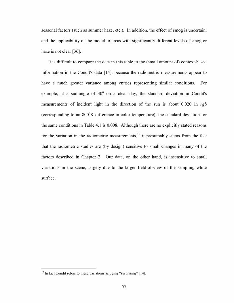
57

seasonal factors (such as summer haze, etc.). In addition, the effect of smog is uncertain,

and the applicability of the model to areas with significantly different levels of smog or

haze is not clear [36].

It is difficult to compare the data in this table to the (small amount of) context-based

information in the Condit's data [14], because the radiometric measurements appear to

have a much greater variance among entries representing similar conditions. For

example, at a sun-angle of 30o on a clear day, the standard deviation in Condit's

measurements of incident light in the direction of the sun is about 0.020 in rgb

(corresponding to an 800oK difference in color temperature); the standard deviation for

the same conditions in Table 4.1 is 0.008. Although there are no explicitly stated reasons

for the variation in the radiometric measurements,19 it presumably stems from the fact

that the radiometric studies are (by design) sensitive to small changes in many of the

factors described in Chapter 2. Our data, on the other hand, is insensitive to small

variations in the scene, largely due to the larger field-of-view of the sampling white

surface.

19 In fact Condit refers to these variations as being “surprising” [14].

58

Sun

Angle Cloud

% Sun

visibility rgbsun σr-sun Vsun σv-sun rgbaway σr-away Vaway σv-away # rgbsky

0-5 0-20 1 .436 .349

.006 195 24 .288 .302

.009 53 29 8 .260 .299

0-5 21-50 1 .436 .349

.006 186 31 .296 .312

.012 48 33 9 .277 .302

0-5 51-70 0.5 .406 .344

.008 158 36 .319 .315

.009 56 38 11 .349 .331

0-5 71-100 0 .352 .335

.005 41 22 .352 .335

.008 41 26 10 .355 .336

6-15 0-20 1 .394 .330

.008 206 31 .288 .302

.010 58 34 6 .274 .305

6-15 21-50 1 .394 .340

.009 198 38 .296 .312

.009 41 40 6 .296 .314

6-15 51-70 0.5 .368 .334

.010 167 29 .319 .315

.012 41 32 7 .331 .330

6-15 71-100 0 .352 .335

.008 44 21 .352 .335

.007 36 24 6 .352 .338

16-25 0-20 1 .385 .337

.008 221 28 .323 .334

.008 51 34 11 .301 .313

16-25 21-50 1 .385 .337

.007 215 26 .323 .334

.013 51 26 7 .334 .323

16-25 51-70 0.5 .376 .337

.011 188 30 .326 .336

.012 58 32 4 .337 .329

16-25 71-100 0 .352 .335

.008 50 21 .352 .335

.009 48 25 4 .357 .335

26-50 0-20 1 .370 .332

.008 224 33 .323 .334

.009 56 35 9 .309 .328

26-50 21-50 1 .370 .332

.007 220 29 .323 .334

.011 69 35 8 .333 .332

26-50 51-70 0.5 .359 .337

.006 176 28 .326 .336

.010 51 31 4 .347 .334

26-50 71-100 0 .352 .335

.008 64 24 .352 .335

.008 68 29 9 .354 .336

51-70 0-20 1 .350 .335

.007 249 36 .323 .334

.010 71 38 3 .312 .330

51-70 21-50 1 .350 .335

.009 249 35 .323 .334

.013 60 37 5 .333 .332

51-70 51-70 0.5 .359 .332

.010 170 37 .326 .336

.010 43 37 9 .341 .332

51-70 71-100 0 .352 .335

.008 52 22 .352 .335

.008 51 25 8 .352 .335

Table 4.1. Context-based illumination model, showing and the rgb and brightness (V) values for the incident light in the direction of the sun (rgbsun, Vsun) and away from the sun (rgbaway, Va rgbaway), for various conditions, along with the corresponding standard deviations and the number of samples (#). The conditions are indexed by the sun angle, the cloud cover (Cloud %) and the sun visibility factor. The last column shows the average color of the sky (rgbsky), measured with the white surface facing up, towards the sky.

59

5 A SURFACE REFLECTANCE MODEL: THE NPF CHAPTER 5

A SURFACE REFLECTANCE MODEL: THE NPF

5.1 Overview

The second model developed in this study is the Normalized Photometric Function, a

reflectance model that is a simplified form of existing models [80] for use in outdoor

color images, and in particular with the daylight model from the previous chapter.

Several physics-based reflectance models exist, most notably Shafer's Dichromatic model

[80], Nayar's hybrid reflectance model [56], and Phong's shading model [70], but these

models make three assumptions that are not suitable for outdoor images. First, they

assume single-source illumination, whereas daylight is a composite illuminant; second,

they require brightness values, and the previous sections showed that the brightness of

daylight is difficult to model; finally, the three models assume that specular surfaces

always demonstrate the characteristic specular effect (the “spike”), which may not be true

if the illuminant is an extended source. This chapter discusses the existing models, and

then derives the Normalized Photometric Function (NPF) through modifications and

simplifications to the existing models, for use in outdoor images. A photometric function

typically plots the brightness of the light reflected off a surface as a function of the

viewing angle; the NPF, however, plots the relative change in normalized color of a

surface as the viewing angle changes.

60

5.2 Existing physics-based models

The Dichromatic Reflectance Model [43][80] represents the intensity of reflected

light (radiance) L, at wavelength λ for a surface at incident angle i, viewing angle e, and

phase angle g as:

L(λ,i,e,g) = ms(i,e,g) cs(λ) + mb(i,e,g) cb(λ) (5.1) where cs(λ) and cb(λ) are the albedos at wavelength λ for the specular and Lambertian

components, respectively; cs and cb are constant for a given surface, and are dependent

only on wavelength—not the illumination or viewing angles. The illumination and

viewing angles determine the geometric scale factors ms(i,e,g) and mb(i,e,g), such that

(0≤ms, mb≤1). The Dichromatic model shows that most of the (i, e, g) combinations will

result in reflectance that is dominated by the Lambertian component, i.e., ms = 0, and

mb = 1. For the remaining angles, depending on the specularity of the surface, (0≤ms,

mb≤1). The points from each of the two components are represented as two linear

clusters in a spectral histogram, which together form a skewed “┴” in a parallelogram

representing the dichromatic plane in RGB space (see Figure 5.1).

61

Figure 5.1. The Dichromatic Model [43][80] describes reflectance in RGB space as a skewed “┴”-shaped cluster within a parallelogram that represents the dichromatic plane.

According to the Phong shading model [70] (adapted for computer vision by Horn

[39]), the brightness of reflectance (L) at incidence angle i, viewing angle e, and relative

viewing angle n (the angle between the directions of viewing and maximal specular

reflection) is:

L(i,e,n) = t n+1

2 cosα (n) + (1–t) cos(i) (5.2)

where t and α are parameters of the material; t represents the total amount of light

reflected by the specular component, and α represents the clustering of reflection of the

specular component about the angle of reflection. In this model the falloff in the

brightness of specular reflection is a function of cosα (n), and the weights for the two

components are t and (1–t). The value of α is determined empirically for a given surface,

and varies from 1 (for matte surfaces) to 200 (for highly specular surfaces). At (n= 0),

the brightness is maximal (i.e., 1), and falls off as the surface is rotated, to the minimum

(i.e., 0) at –90o and 90o.

cs

R

G

B

cb

Pixel values

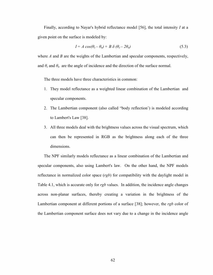
62

Finally, according to Nayar's hybrid reflectance model [56], the total intensity I at a

given point on the surface is modeled by:

I = A cos(θs – θn) + B δ (θs – 2θn) (5.3)

where A and B are the weights of the Lambertian and specular components, respectively,

and θs and θn are the angle of incidence and the direction of the surface normal.

The three models have three characteristics in common:

1. They model reflectance as a weighted linear combination of the Lambertian and

specular components.

2. The Lambertian component (also called “body reflection’) is modeled according

to Lambert's Law [38].

3. All three models deal with the brightness values across the visual spectrum, which

can then be represented in RGB as the brightness along each of the three

dimensions.

The NPF similarly models reflectance as a linear combination of the Lambertian and

specular components, also using Lambert's law. On the other hand, the NPF models

reflectance in normalized color space (rgb) for compatibility with the daylight model in

Table 4.1, which is accurate only for rgb values. In addition, the incidence angle changes

across non-planar surfaces, thereby creating a variation in the brightness of the

Lambertian component at different portions of a surface [38]; however, the rgb color of

the Lambertian component surface does not vary due to a change in the incidence angle

63

(as long as the illuminant color does not change).20 As a result, the NPF model can easily

be applied to non-planar surfaces.

There are also three notable differences between the three models:

• The Phong model assumes that the weights of the two components are dependent

(t and (1–t)); as described by Horn [39], this is because if an amount t of the

incident light in reflected by the specular component of the surface, the remainder

of the light (which is (1–t)) penetrates to the “body” of the surface21 and exhibits

Lambertian reflectance. On the other hand, Shafer and Nayar do not explicitly

assume dependency between the coefficients of the two components.

• The brightness falloff models for the specular component are different: Nayar

uses the delta function [57], Phong uses cosαn, and Shafer does not specify the

specular falloff function.

• Phong and Nayar, unlike Shafer, develop a photometric function.

Because it predicts reflectance in normalized color space, the NPF assumes that the

sum of the weights of the two components is 1. It is then shown that based on a

simplification of the Dichromatic model, the composite falloff function, i.e., the transition

between the color of the Lambertian component and the color of the specular component

(as the surface orientation changes) is along a straight line in rgb color space. Based on

the straight line, a piecewise-linear photometric function is empirically derived, mapping

20 Note that the NPF ignores the effect of intensity, separating surface intensity from normalized color; however, one of the pixel classification techniques described in Chapter 6 explicitly uses intensity constraints. 21 Phong describes specularity as light reflecting off a thin, smooth outer layer of a surface, and Lambertian reflection as resulting from penetration of light through the outer layer to the rougher “body” of the surface.

64

the relative viewing angle (which is the angle between the directions of viewing and

maximal specular reflection) to the relative change in the weights of the two components.

As described earlier, there are three reasons the aforementioned three physics-based

models are difficult to use—in their current form—for color recognition in outdoor

images. First, all three models assume a single-source illuminant (either point or

extended).22 The second reason is with regard to ms (to use the terminology of the

Dichromatic Model), the scale factor of the specular component. In the physics-based

models, ms is modeled either as an impulse function of i and e [46][56] or as a power of

cos(n) [70]. Intuitively, this means that all surfaces with (cs(λ) > 0) (i.e., all surfaces with

a specular component) will exhibit the specular “spike”, which is modeled by ms(i,e,g).

Under daylight, the specular effect is apparent only under bright sunlight, but is

diminished or absent under only skylight or under an overcast sky. Hence, the effect of

the illuminant (i.e., the presence, obscuration of, or absence of the sun) on the specular

component must also be taken into account. The third reason the existing models need to

be modified is that all three reflectance models deal with intensity values, which are

independently calculated for each of the R, G, and B primaries when applied to color.

The CIE daylight model and the model in Table 4.1 explicitly avoid intensity-based

modeling, because the intensity of incident daylight is difficult to precisely model. In

addition, as mentioned before, the brightness of the Lambertian component varies over

the area of non-planar surfaces; this means that using a non-normalized space would

22 Sato [77] adapts a general weighted linear reflectance model for shape recovery under daylight, and applies it to shape recovery by modeling sunlight as a “narrow Gaussian distribution”. In that model, Lsun(θi-θs) = A exp (-(θi-θs)2/(σ2)), where Lsun is the intensity of sunlight with incidence angle θi and reflecting angle s. The term σ represents the standard deviation of the distribution, and A is an empirical parameter. However, the model requires bright sunlight without any clouds, and does not account for the effect of a cloud cover or sun-obscuration (partial or full).

65

require knowledge of the surface normal at every point on the surface. On the other

hand, he normalized rgb color does not change due to a change in the incidence angle

under a given illuminant. Hence, although these reflectance models have been used

successfully for problems such as shape-from-shading (Nayar) and estimation of

reflectance and illumination parameters (Shafer), and for rendering synthetic images

(Phong), they have to be modified for use in outdoor images with a model of daylight.

5.3 Derivation of the NPF

As mentioned earlier, the NPF combines aspects of the three physics-based models,

so that it can be applied to a model of daylight such as the one in Table 4.1. To begin

with, the NPF separates the effect of intensity from that of normalized color. The NPF

can be derived from the Dichromatic Model, which does not explicitly assume that the

coefficients of the two components are dependent. In the Dichromatic Model, the

condition (0 ≤ ms, mb ≤ 1) is true, but the condition (ms + mb = 1) is not assumed to be

true; in other words, the model assumes that the scale factors of the two components are

mutually independent. With the exception of some surfaces (such as fluorescent paints

and certain metals [32]), specular surfaces typically reflect back the color of the

illuminant, with a uniform albedo; hence, cs(λ) = 1.

In addition, it can be shown that for normalized color, the condition (ms + mb = 1) is

valid.23 According to the weighted-combination reflectance models, in RGB, Ra = WlRl +

WsRs, Ga = WlGl + WsGs, and Ba = WlBl + WsBs, where Ra, Ga and Ba are the apparent

colors of the surface, Rl is the albedo of the red component Lambertian, Wl the weight of

23 Note that this assumption is made in the intensity-based models derived by Phong [70] and Horn [39].

66

the Lambertian component, and so on. In rgb, r = R/(R+G+B). Hence,

sBsGsR

sRsW

lBlGlR

lRlWar

+++

++= . If the two weighted components are multiplied by

some constant A (representing intensity), then R, G and B all become multiples of A, thus

leaving the ratio [R:G:B] unchanged. Hence, multiplying the components by a constant

does not alter ra, ga, or ba. Since the constants do not affect the apparent normalized

color, the ratio of the weights are what matter, not their absolute values. This means that

the weights are not independent. Hence, if both components were multiplied by the

expression (1/Wl), Wl would be replaced by 1, and Ws by (Wl/Ws). By the same token, the

sum of the weights, Wl+Ws, can be set to a constant; when that constant represents

maximal reflectance, the constant can be set to 1, with sub-maximal reflectance

represented by fractions between 0 and 1. Hence, it can be assumed that the condition

(Wl + Ws = 1) is valid.

Physically, if the specular component reflects the color of the illuminant, then a pure

specular surface with ms=1 and mb=0 will be the color of the illuminant. As the weight of

Lambertian component increases (with a change in the viewing angle), the apparent color

of the surface tends away from the color of the illuminant towards the color of the

Lambertian component. Hence, ms decreases as mb increases. In the extreme, if the

surface is Lambertian, ms=0 and mb=1, and the apparent color of the surface is the

apparent color of the Lambertian component. This observation, also made by Horn [39],

makes (ms + mb = 1).

Therefore, in rgb the Dichromatic Model can be simplified to:

L(λ,i,e,g) = (1–mb(i,e,g)) + mb(i,e,g) cb(λ)

67

Note that (as explained earlier in this section) the expression cs(λ) is eliminated from the

model because the specular component reflects back the color of the illuminant, meaning

that cs(λ) = 1 . Further, the Dichromatic Model uses the phase angle g as a third angular

parameter, in addition to the incidence angle i and the viewing angle e. According to the

Lambertian model [38], the brightness—not the normalized color—is a function of the

phase angle. Hence, g can be simplified as the sum of i and e. Finally, by expressing the

combination of i and e as the relative viewing angle n, i.e., the difference between the

viewing angle and the angle of maximal specularity (as in the Phong model), the

Dichromatic Model can be normalized to:

L(λ,n) = (1–mb(n)) + mb(n) cb(λ) (5.4)

In Equation 5.4 the Lambertian component is defined in the wavelength space.

According to the Lambertian model, the energy reflected at a given wavelength λ is

measured as the product of the incident light and the surface albedo [38]:

ρ(λ) = ι(λ) cos(θi) σ(λ) (5.5) where ρ(λ) and ι(λ) denote the intensity of the reflected and incident light at wavelength λ,

respectively, θi is the angle of incidence, and σ(λ) is the surface albedo for light at

wavelength λ. In a normalized color space, the brightness component of the Lambertian

model is eliminated. Hence, the cosine factor in Equation 5.5 is dropped:

ρ(λ) = ι(λ) σ(λ) (5.6)

Equation 5.6, which uses the continuous wavelength space, can be reduced to the

three-dimensional rgb space by using a set of three camera/digitizer filters (which, the

reader may recall, are linear transforms of the CIE tristimulus functions [32], but need to

be calibrated for each individual camera), and then normalizing over intensity, to get:

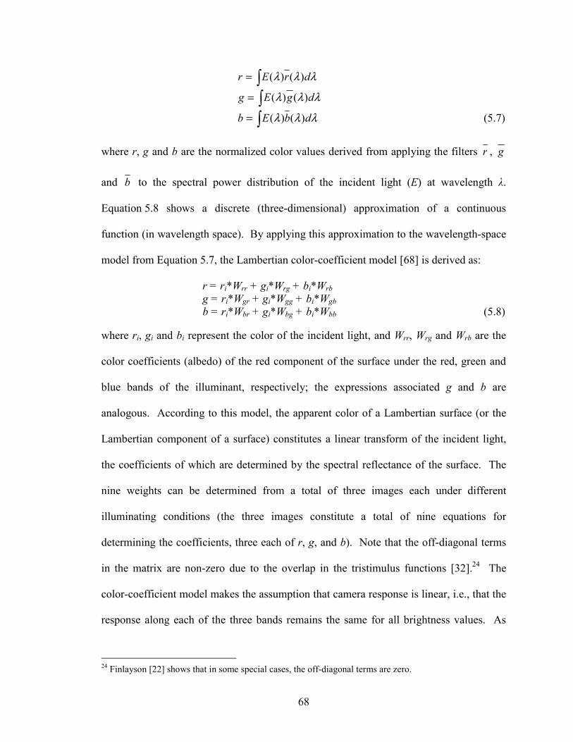
68

λλλ drEr )()(∫=

λλλ dgEg )()(∫=

λλλ dbEb )()(∫= (5.7)

where r, g and b are the normalized color values derived from applying the filters r , g

and b to the spectral power distribution of the incident light (E) at wavelength λ.

Equation 5.8 shows a discrete (three-dimensional) approximation of a continuous

function (in wavelength space). By applying this approximation to the wavelength-space

model from Equation 5.7, the Lambertian color-coefficient model [68] is derived as:

r = ri*Wrr + gi*Wrg + bi*Wrb g = ri*Wgr + gi*Wgg + bi*Wgb b = ri*Wbr + gi*Wbg + bi*Wbb (5.8)

where ri, gi and bi represent the color of the incident light, and Wrr, Wrg and Wrb are the

color coefficients (albedo) of the red component of the surface under the red, green and

blue bands of the illuminant, respectively; the expressions associated g and b are

analogous. According to this model, the apparent color of a Lambertian surface (or the

Lambertian component of a surface) constitutes a linear transform of the incident light,

the coefficients of which are determined by the spectral reflectance of the surface. The

nine weights can be determined from a total of three images each under different

illuminating conditions (the three images constitute a total of nine equations for

determining the coefficients, three each of r, g, and b). Note that the off-diagonal terms

in the matrix are non-zero due to the overlap in the tristimulus functions [32].24 The

color-coefficient model makes the assumption that camera response is linear, i.e., that the

response along each of the three bands remains the same for all brightness values. As

24 Finlayson [22] shows that in some special cases, the off-diagonal terms are zero.

69

discussed in Chapter 2, the response function for cameras can be nonlinear, and is a

function of the gamma-correction (γ) factor. For each of the bands, the output signal o is

determined by (o = iγ), where i is the strength of the input signal on the digitizer, and γ,

the gamma-correction factor. Fortunately, it is not difficult to linearize the response [60]

(for some cameras, it is possible to simply disable the gamma-correction). For the data

collected for this study, the camera f-stop was adjusted so as to restrict the response to a

very small range in the middle, approximately linear portion of the response function.

In matrix notation, the color-coefficient model is represented as:

=

i

i

i

bbgbbr

gbgggr

rbrgrr

bgr

WWWWWWWWW

bgr

(5.9)

Earlier, in Equation 5.4, the Lambertian component was represented by mb(n)cb(γ),

which is the wavelength form of the color-coefficient model shown in Equation 5.9,

above. In the normalized rgb space, the apparent color of this component is a single

point determined by applying the color-coefficient matrix to the normalized color of the

illuminant. The specular component, represented in Equation 5.4 simply as (1-mb(n)), is

an offset from the point (in the direction of the illuminant rgb color) that represents the

apparent normalized color of the Lambertian component; Figure 5.2 shows this

phenomenon.

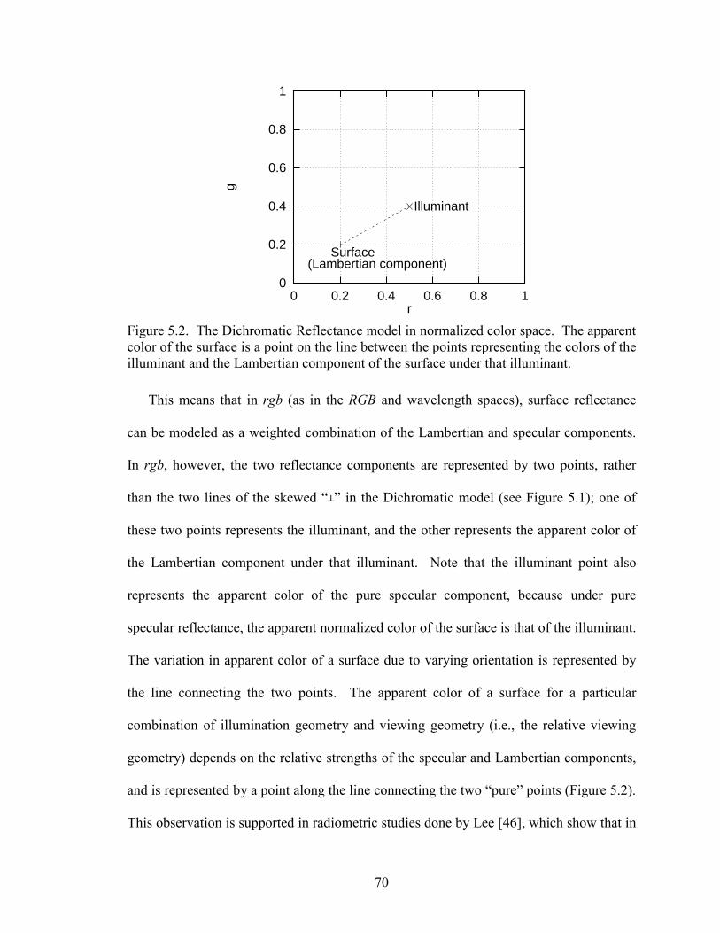
70

0

0.2

0.4

0.6

0.8

1

0 0.2 0.4 0.6 0.8 1

g

r

Illuminant

Surface(Lambertian component)

Figure 5.2. The Dichromatic Reflectance model in normalized color space. The apparent color of the surface is a point on the line between the points representing the colors of the illuminant and the Lambertian component of the surface under that illuminant.

This means that in rgb (as in the RGB and wavelength spaces), surface reflectance

can be modeled as a weighted combination of the Lambertian and specular components.

In rgb, however, the two reflectance components are represented by two points, rather

than the two lines of the skewed “┴” in the Dichromatic model (see Figure 5.1); one of

these two points represents the illuminant, and the other represents the apparent color of

the Lambertian component under that illuminant. Note that the illuminant point also

represents the apparent color of the pure specular component, because under pure

specular reflectance, the apparent normalized color of the surface is that of the illuminant.

The variation in apparent color of a surface due to varying orientation is represented by

the line connecting the two points. The apparent color of a surface for a particular

combination of illumination geometry and viewing geometry (i.e., the relative viewing

geometry) depends on the relative strengths of the specular and Lambertian components,

and is represented by a point along the line connecting the two “pure” points (Figure 5.2).

This observation is supported in radiometric studies done by Lee [46], which show that in

71

the CIE chromaticity space, the reflectance of various surfaces form straight lines which

converge at the point representing the illuminant.

Applying Equation 5.4 to the tristimulus functions shown in Equation 5.7 and to the

color-coefficient model in Equations 5.8 and 5.9:

A(n) = C + [I-C]*ρ (5.10) where A is the apparent rgb color (vector) of a surface at a relative viewing angle n, under

illuminant color (vector) I, with a Lambertian component vector C, at relative distance ρ

between C and I.

5.4 The photometric function

A photometric function typically profiles the change in surface reflectance intensity

as the viewing angle changes, where the vertical axis represents the range between

minimal and maximal intensity. Since the normalized rgb color of a surface is

constrained to be on the line between the color of its Lambertian component and the color

of the illuminant (i.e., the normalized dichromatic line shown in Figure 5.2), the NPF

relates the viewing angle to the point on this line. Hence, the vertical axis of the NPF

represents the relative change in normalized color between the color of the illuminant and

the color of the Lambertian component of the surface. Equation 5.10 is the basis for the

Normalized Photometric Function, which maps the weights of the two reflectance

components (i.e., the relative distance along the dichromatic line) as a function of the

relative viewing angle. Hence, the horizontal axis represents the relative viewing angle

(the term n from Equation 5.10), which ranges from -90o and 90o. At n = 0o, the viewing

angle equals the angle of maximal specularity. The vertical axis, scaled from 0 to 1,

72

represents the relative distance (the term ρ from Equation 5.10) between the color of an

illuminant and the apparent color of the Lambertian component of the surface under that

illuminant.

Rel

ativ

e rg

b D

ista

nce

(

)

Sunlight Skylight

ρh

-90

Relative Viewing Angle (n)

900

ρ

Skylight

Spec. Comp. under Sunlight

Lamb. Comp. under Skylight

-n nhh

Figure 5.3. The theoretical NPF for a surface with both Lambertian and specular components, under daylight while facing the sun. The distance between the upper and lower lines (ρ) represents the relative distance between the normalized colors of the illuminant and the Lambertian component of the surface under that illuminant. As the relative viewing angle approaches 0o, the apparent color of the surfaces with a specular component approaches the color of the illuminant. The height of the NPF peak depends on the specularity of the surface and the visibility of the sun. The width of the peak can be different at its apex and base: the width of the peak apex depends on the angle subtended by the sun, and is assumed constant at 0.5o for all surfaces with a specular component. The width of the peak base depends on the surface roughness; it is about 0.5o for a perfectly smooth specular surface (same as the peak apex), and wider for rougher specular surfaces.

5.4.1 Empirically obtaining the NPF for particular surfaces

This section describes the process of empirically obtaining the NPF for given

surfaces, including determining the width and height of the specular peak. It is shown in

Chapter 6 that every pixel in the image is at a different viewing angle with respect to the

surface normal; hence, the relative viewing angle and consequently the apparent color of

a surface changes over image pixels. Hence, if a surface is large enough (and depending

73

on the camera field-of-view), its NPF can be estimated from a single image with the

surface facing the sun (i.e., with an incident angle of 0o). However, if the surface is not

large enough, multiple images are required, so that the entire -90o to 90o range can be

measured.

For a given image, the color of the illuminant is determined from the daylight table,

based on which the apparent color of the Lambertian component is estimated using the

color-coefficient model. The portion of the row of pixels on the surface passing through

the centroid, is then selected, and for each pixel, the value of ρ (i.e., the relative position

of the pixel's rgb, between the Lambertian and illuminant rgb points) is mapped against

the relative viewing angle at that pixel, based on the surface's rgb value at that pixel.

Depending on the relative strengths of the Lambertian and specular components of a

surface, three cases are possible:

• If the Lambertian component is dominant for all viewing angles, there is no

change in the apparent color of the surface, even as the relative viewing angle (n)

changes from -90o to 0o, and eventually to 90o; the color is always that of the

Lambertian component under that illuminant. The scale factor mb from

Equation 5.4 equals 1, and ms = 0. Hence the value of ρ for the NPF stays at 0 for

the whole range of viewing angles.

• If both reflectance components are strong (as shown in Figure 5.3), when n is -90o

mb = 1, and the apparent color of the surface is the apparent color of the

Lambertian component under the illuminant. It stays that way until n approaches

0o, at which point mb decreases to some fraction (say, ρh) such that (0 ≤ ρh ≤1),

and ms undergoes a corresponding increase to (1-ρh). The precise value of ρh will

74

depend on the specularity of the surface and on the sun-visibility factor from

Table 4.1 (this phenomenon is discussed shortly). Notice that ρ changes to ρh at

some point (-nh < 0o), rather than at (nh = 0o). This is because the sun is an area-

source illuminant, not a point-source;25 for (n ≥ nh), ρ = 0. The width of the peak

is also a function of the surface roughness; this phenomenon is also described

shortly.

• For surfaces with a dominant specular component, the only difference is that for

(–nh > n > nh), ρ = 1, since ms = 1 and mb = 0. In the special case where (cb(λ) =

0), which happens for perfect mirrors, at all (n ≥ (–nh) and (n ≤ nh), no light is

reflected from the surface.

The NPF peak under daylight is a plateau, where the width of the apex of the peak is

different from the width of the base. In other words, the bottom of the peak starts at –nh

and the plateau (the flat top of the peak) may start at some point –np, such that the

condition (–nh < –np < 0) is true. The width of the apex depends on the angle subtended

by the sun, which is assumed constant at 0.5o [98]. Hence the NPF's for all surfaces with

a specular component have a peak apex range of 0.5o. The width of the base of the NPF

peak (i.e., the range (–nh to nh)) depends of the surface roughness, and is similar to the α

factor in the Phong model. As in the Phong model, this factor is empirically derived for

the NPF of each surface. For a perfectly smooth specular surface, the width of the peak

base is the same as the width of the peak apex, which is 0.5o. For an imperfectly smooth

surface such as a traffic sign, the base of the peak was empirically found to span a range

25 In the case of a point-source illuminant, (ρ = 0) for all (–90o ≤ n < 0o) and for (n > 0o); at (n = 0o), ρ equals ρh.

75

of about 4.5o. For imperfectly specular surfaces (i.e., with some roughness, such as a

slightly worn shiny plastic surface), the base width was found to be about 7.2o.

Note that the width of the NPF peak is not just a property of the surface, but

specifically of the surface reflectance under daylight. In other words, the width may be

different under a different illuminant. The slope of the NPF peak (i.e., ρh/(nh–np))

depends on the relative widths of the peak's apex and base, and hence is also a property

of the surface and its reflectance under the illuminant. The slope of the peak also

depends on another characteristic of the illuminant—the color gradient between the

sunlight and skylight. Intuitively, the sharper the color gradient, the sharper the slope.

For instance, if the boundary between the sun and sky is “blurred” (due to sun

obscuration), the slope is “gradual”; if the boundary is sharp, the slope is “steep”. A

formal method for determining the slope of the peak is not presented because the NPF for

a given surface is derived empirically from samples of daylight and the target surface. In

addition, one problem with measuring and estimating the slope of the peak is that the

pixels representing the gradient can be affected by color-mixing due to pixel interpolation

by the camera, and hence may not be reliable.

Hence, the NPF of a surface has eleven free parameters: nine are the Lambertian

weights from the color coefficient matrix, and the other two are the height of the apex

and the width of the base. Note that the width of the apex will always be 0.5o under

daylight. It was mentioned earlier that the nine weights are derived from three images;

the following discussion describes the process for empirically estimating apex and base

widths.

76

Figure 5.4 and Figure 5.5 show the NPF's for five surfaces under daylight facing the

sun: matte paper, two traffic signs, a concrete slab, and a slab of road asphalt. The NPF

for each surface was determined from three images of which the first image had a relative

viewing angle of 0o with respect to the surface normal at the centroid of the surface.

Depending on the size of the surface, this encompassed a range of viewing angles

between –10o and 10o for the largest surface (the “Stop” sign), and between –5o and 5o for

the smallest (the matte paper). The NPF was determined—as described before—by

selecting a row of pixels passing through the centroid of the surface and measuring the

rgb values of the pixels on the surface. Thereafter, the data is plotted as a two-

dimensional function, with the relative viewing angle on the horizontal axis and the

distance between the rgb colors of the illuminant and the Lambertian component under

that illuminant along the vertical axis. In order to reduce the effect of pixel-level noise,

the value at each pixel is taken as the average over a 3×3 neighborhood. None of the five

surfaces are large enough to encompass a range of viewing angles larger than –10o to 10o;

hence, to measure the apparent color of the surfaces outside the range available from a

single image, the viewing angle was changed so as to incorporate the entire –90o to 90o

range.

An NPF is fitted to the data according to the one of two conditions:

1. If a single straight line at ρ = 0 can be fitted to all the points (with a statistically

significant goodness-of-fit or R2, based on the noise model described in

Chapter 6), that line defines the NPF for the surface. This means that the surface

has a negligible specular component.

77

2. Otherwise, it is concluded that the surface has a specular component, and that the

NPF should have a peak. As described earlier, the width of the apex of the peak

is constant for all surfaces under sunlight, and the width of the base of the peak is

empirically determined. The samples of the surface are then used to determine

the height of the peak: A single straight line at ρ = 0 is fitted to points in a range

of angles (–90o ≥ θ ≥ –nh), and a second straight line is fitted to the two points at θ

= nh and θ = 0.5o. Then, if this set of two lines can be symmetrically fit across the

θ = 0o axis to the remaining points, the symmetric piecewise linear function

defines the NPF for the surface.

The above process was applied to each of the surfaces in shown Figure 5.4 and Figure

5.5 (matte paper, “Stop” sign, “No Parking” sign, concrete slab and road asphalt), the

average RMS errors from using the above procedure to fit the NPF's were 0.007, 0.013,

0.081, 0.108, and 0.113, respectively. For each surface, the NPF fit was calculated over

17 points at various relative viewing angles. The errors from fitting the sampled data to

the NPF model are greater for the slab of concrete and asphalt and the “No Parking” sign,

than for the other two surfaces. This is because the concrete, asphalt and the “No

Parking” sign are neutral-colored (grey and white, respectively) which means that their

apparent color is always close to the color of the illuminant. Since the points

representing the illuminant and the Lambertian component under the illuminant are very

close to each other in rgb space, even small errors in rgb appear magnified relative to the

total distance between the two points.

The height of the NPF in outdoor images also depends on two other factors: the

illumination geometry and the visibility of the sun (as defined in Table 4.1). When the

78

surface faces away from the sun, the conditions causing the specular peak do not exist,

and there is no specular peak. On the other hand, if the surface faces the sun, but the sun

is behind a cloud, the specular peak either completely disappears, or is reduced in height,

depending on the thickness of the cloud. Hence, it is necessary to scale the NPF based on

the illumination. Although it is difficult to predict the precise effect of the sunlight on the

specular peak, an approximate estimate is made using the sun-visibility factor. The

scaling is done by multiplying the height of the NPF peak by the sun-visibility factor.

The data in Figure 5.6 was collected from images of the two traffic signs under a cloudy

sky, with the sun-angle at 27o and a sun-visibility factor of 0.5 (see Table 4.1 for more

information about those conditions). Figure 5.6(a) shows rgb color of the “No Parking”

sign, plotted relative to the distance from the illuminant color; the figure also shows an

NPF, scaled by the sun-visibility factor of 0.5. Figure 5.6(b) shows the sampled data and

the NPF scaled at 0.5 for the “Stop” sign. The RMS errors between the sampled data and

the scaled NPF's for the two surfaces were 0.144 and 0.073, respectively. Note that the

NPF's for only those surfaces with a specular peak (when a single straight line cannot be

fitted to the photometric data) need illuminant-based scaling.

Note that the ability of an illuminant to cause a specular peak should not be confused

with the ability to cause specular reflection. A specular surface will always exhibit

specular reflection—the specular peak associated with that reflectance will be visible

only under a single-source illuminant (point or otherwise), or under daylight when

sunlight is incident. Under an ambient illuminant (such as skylight), there will be

specular reflection at every viewing angle and hence there will be no single peak.

79

The NPF model is used to first determine the apparent color of the Lambertian

component (using the color-coefficient matrix), and the offset in the direction of the

illuminant. It was mentioned earlier that the color-coefficient matrix can be estimated

from three sample images. In order to determine the width of the NPF peak (given the

size of the surface and the surface-camera distance), and the maximum height of the NPF

peak (which can then be scaled based on the sun visibility), a fourth sample image is

required, under conditions resulting in maximal specularity for the surface (i.e., at a

relative viewing angle of 0o, facing the sun with a visibility factor of 1). For each of the

surfaces in Figure 5.4 and Figure 5.5, the NPF's are estimated from four images. In

Chapter 6 these NPF's are combined with the daylight model for estimating the apparent

color of the five surfaces under various conditions, and the estimates are used for

classifying image pixels.

80

-90 -60 -30 0 30 60 90

Relat

ive rg

b dist

ance

Relative viewing angle

0

1

(a) Matte paper

-90 -60 -30 0 30 60 90

Relat

ive rg

b dist

ance


0

1

(b) Concrete slab

-90 -60 -30 0 30 60 90

Relat

ive rg

b dist

ance


0

1

(c) Road asphalt

Figure 5.4. Normalized Photometric Functions for three of the five sample surfaces (under daylight, facing a bright sun): (a) matter paper, (b) concrete slab, (c) road asphalt.

81

-90 -60 -30 0 30 60 90

Relat

ive rg

b dist

ance


0

1

(a) “No Parking” sign

-90 -60 -30 0 30 60 90

Relat

ive rg

b dist

ance


0

1

(b) “Stop” sign

Figure 5.5. Normalized Photometric Functions for the remaining two of the five sample surfaces (under daylight, facing a bright sun): (a) “No Parking” sign, (b) “Stop” sign.

82

-90 -60 -30 0 30 60 90

Relat

ive rg

b dist

ance


0

1

(a)

-90 -60 -30 0 30 60 90

Relat

ive rg

b dist

ance


0

1

(b)

Figure 5.6. NPF's for the traffic signs facing the sun under partly cloudy sky: (a) “No Parking” sign, (b) “Stop” sign.

83

6 ESTIMATING APPARENT NORMALIZED COLOR CHAPTER 6

ESTIMATING APPARENT NORMALIZED COLOR

6.1 Overview

As mentioned earlier, one motivation for developing models of daylight color and

surface reflectance is to predict apparent surface color in outdoor images. While the

previous two chapters introduced a model of daylight color and a surface reflectance

model represented by an NPF, this chapter describes the process of combining the two

models to estimate apparent color.

Note that the NPF uses the relative viewing angle, which, as the reader may recall,

combines the illumination and viewing angles; however, these angles may not always be

known. Hence, this section develops methods for estimating apparent color under two

scenarios: when the relative viewing angle is known (Section 6.2) and when it is

unknown (Section 6.3). Section 6.4 develops a method for classifying image pixels based

on the estimated apparent color, and the probability that a given image pixel is the same

color as the estimate, within the constraints of the noise model. A total of 90 images

under different conditions are used to test the methods; these conditions are described

(along with the results) in the sections discussing each of the sample surfaces.

6.2 Estimating apparent color when the relative viewing angle is known

When the relative viewing angle (in addition to the daylight conditions and surface

reflectance) is known, it is possible to use the daylight table (Table 4.1), along with the

color-coefficient and NPF models to estimate the apparent color. In the absence of noise

or other sources of error, this prediction is an rgb point on the normalized dichromatic

84

line. In practice, however, there are three sources of error: the models of daylight and

surface reflectance, and the relative viewing angle. Since the color of the incident light is

estimated from the empirical measurements in Table 4.1 (which have non-zero errors),

the error associated with this estimation is approximated as a Gaussian distribution, the

standard deviation of which equals that of the measurements shown in Table 4.1. The

error in estimating the NPF for each surface is also modeled as a Gaussian, the standard

deviation of which is derived empirically using the method described in the next section.

Finally, because the relative viewing angle is provided by a user or an external system

(not estimated from data), the user must provide an estimate of its accuracy. An error in

the estimate of the relative viewing angle changes the estimate of the apparent color from

a point on the dichromatic line to a segment of the dichromatic line; the magnitude of the

error determines the length of the line-segment. Note that if the NPF function is flat

around the estimated relative viewing angle,26 then the prediction will be a point in rgb,

and the error model reduces to a Gaussian distribution around a point; this, however, is a

special case. In the general case, the error model for predicting apparent color is a

Gaussian distribution that combines the errors associated with the estimates of the

illuminant color and the surface reflectance models, centered around a line of possible

apparent colors generated by the uncertainty in the relative viewing angle. In other

words, it is a Gaussian distribution centered around a segment of the normalized

dichromatic line.

26 This can happen due to three reasons: (a) because the surface is Lambertian, (b) because the sun is not visible, or (c) because the relative viewing angle is outside the specular range.

85

6.2.1 Deriving the Gaussian noise model

The probability distribution representing the composite error from the three sources is

derived by convolving the individual errors from each source. The error from the

daylight model for the gamut of conditions was shown in Table 4.1 to be about 0.007

(and assumed symmetric along r and g). The second source of noise is the NPF, the error

from which was determined in a test over the five target surfaces. For each surface, the

color-coefficient matrix and NPF were estimated and then used to predict the apparent

color of the surfaces under three different conditions with known illuminant color (for a

total of 15 tests). Note that while estimating the average error of the reflectance, the

color of the incident light was measured directly by placing the white surface in the

image, not from Table 4.1. This was done in order to separate the errors due to the

reflectance model from errors in the daylight model. When the Gaussians representing

the errors from the daylight and reflectance models are convolved, the result is another

Gaussian representing the composite error from the two sources. This composite

Gaussian represents the overall error model around an rgb point (the Lambertian point on

the dichromatic line) when the NPF at the relative viewing angle is flat (as discussed

above). If the NPF has a peak, the apparent color of the surface is a point on the

dichromatic line, and the error model is a Gaussian distribution around a segment the

dichromatic line. The error associated with the relative viewing angle is a one-

dimensional Gaussian, which is incorporated into the composite error model by

convolution with the two-dimensional Gaussian (representing the errors from the

reflectance and daylight models). The probability distribution representing the composite

of these two Gaussians is estimated by separating the two-dimensional Gaussian into the

86

two orthogonal dimensions, one along the dichromatic line and the other along the

normal to the dichromatic line. Thereafter, the one-dimensional Gaussian from the

relative viewing angle error is convolved with one-dimensional Gaussian along the

dichromatic line, resulting in a composite one-dimensional Gaussian. Finally, this

Gaussian is convolved with the one-dimensional Gaussian orthogonal to the dichromatic

line, resulting in a composite two-dimensional asymmetric probability distribution which

represents the error associated with the combination of the three sources. In the examples

to follow, the error in estimating the viewing angle is assumed to be 1o, based on multiple

measurements and the resultant average errors.

6.2.2 The viewing angle at each pixel

��

��

��

��

Focalpoint Optical axis

Surface normal

θα

φ

Surf

ace

View ray

Image plane

Pixel at (r, c)

Figure 6.1. Viewing geometry for image pixels: The viewing angle(φ) for a pixel at position [r,c] equals (90 + α - θ), where θ is the angle between the optical axis and the surface normal, and α is the angle of the viewing ray at pixel [r,c], which is determined the field-of-view of the camera.

The next step in estimating the apparent color of the surface is determining the

viewing angle at each pixel in the image. Different image pixels will have different

relative viewing angles (the angle between the surface normal and the viewing ray).

Since the viewing angle for specular surfaces determines the relative strengths of the

reflectance components, it is possible for some pixels on the surface to exhibit

87

specularity, while other pixels on the surface do not. Figure 6.1 describes the geometry

used for estimating the viewing angle at individual pixels. In this figure, θ represents the

angle between the surface normal and the optical axis. All viewing rays not parallel to

the optical axis will have different angles with respect to the surface normal; this angle is

a function of the position of the pixel (row and column) and the field-of-view of the

camera. For the camera used in this study, the field-of-view (horizontal) was 45o, with

the image being 504 pixels wide; hence it was assumed that the optical axis goes through

the 252nd column27, and a ray going through a pixel in column c will be at a 22.5252

c252×

−

degree angle with respect to the optical axis. In addition to θ, Figure 6.1 shows two

other angles: α is the angle between the optical axis and the viewing ray at a pixel [r,c],

and φ is the angle between the ray and the surface, if the two intersect. In other words, if

the ray going through [r,c] intersects the surface, the viewing angle for [r,c] will be φ; if

the ray does not intersect the surface, the question of an angle between the ray and the

surface does not arise. Geometrically, φ = 90 + α - θ. The relative viewing angle is the

difference between the angle of incidence and the viewing angle.

The relative viewing angle at each pixel in the image is determined, and the target

surface's NPF is used to estimate the apparent rgb color that the surface would be, if it

were at that particular pixel. Thereafter, the estimated rgb value at a given pixel is

compared to the actual rgb value of that pixel; if the pixel is on the target surface, the

accuracy of the estimation is measured by several performance metrics. If, on the other

27 This assumes that the camera is properly aligned, with no spherical distortion. In practice the true optical center may range from one pixel left or right (or up or down) for scientific quality cameras (with a small possible error in estimating the angle), to potentially more for lower quality cameras. Calibration will help reduce the effect of such distortions.

88

hand, the pixel is not on the surface, the question of evaluating the estimation accuracy

does not arise.

6.2.3 Results

The tests over 90 images of the five surfaces can be grouped according to

performance into two categories: the results for the matte paper, the “No Parking” sign

and the “Stop” sign showed a high level of accuracy, while those for the concrete and

asphalt slabs were not as accurate. The following is a discussion of the tests and an

analysis of the results. In the discussion, the accuracy of the estimate is measured by the

number of observed samples found to be within the confidence interval of the estimate.

In addition, the certainty of the estimation is measured by the area of rgb space within the

2σ confidence interval; in other words, the smaller the area of the interval is, the tighter—

and more useful—the constraint imposed by the confidence interval will be.

6.2.3.1 Matte paper

For the matte paper, tests were conducted on 20 images over 4 sets of conditions

(Table 6.1). Since the surface does not have a specular component, each set of conditions

has a single estimated rgb color, which is the apparent color of the Lambertian

component. For each of the 20 images, the actual color of the surface was determined by

averaging a 20×20 region of the image. All 20 observed values were within the 2σ

confidence interval of the estimates under the corresponding conditions. On average, the

estimated rgb was 0.005 away from the observed rgb. Figure 6.2 shows the confidence

interval about the estimate under each of the four sets of conditions, along with the

89

observed rgb values for all the images under each set.28 The area within the interval (i.e.,

the certainty of the estimate) was about 0.0002 square units (where the confidence

interval is a circle with a radius of about 0.008). One reason for the accuracy of the

estimate is that the surface is Lambertian, as a result of which the errors due to the NPF

and the viewing angle are eliminated.

28 Section 6.4 discusses the appropriate confidence intervals to be used in the context of pixel classification.

90

Sun angle

Illumination angle

Viewing angle

% Cloud cover

Sun visibility factor

# Samples % Observations within CI

Average error

10 0 0 0 1 5 100% 0.004 35 10 0 0 1 4 100% 0.006 50 0 50 80 0 6 100% 0.004 60 180 80 20 1 5 100% 0.005

Table 6.1. Results of apparent color estimation (with known relative viewing angle) for the matte paper. Four sets of conditions were sampled, with each row describing the sun angle, illumination angle, viewing angle, approximate cloud cover, and the sun visibility factor for the corresponding set of conditions. For each set of conditions, the number of samples are shown, along with the percentage of observations that fell within the estimated confidence interval, and the average error from the estimate.

0.3

0.325

0.35

0.35 0.4 0.45 0.5

g

r

Set 1Set 2Set 3Set 4

Figure 6.2. Estimates of the apparent color of the matte paper under four sets of conditions are represented by the corresponding confidence intervals. As the figure shows, 100% of the actual observed colors are within the estimated confidence intervals.

91

6.2.3.2 “No Parking” sign

Sun angle

Illumination angle

Viewing angle

% Cloud cover


Effect # Samples

% Observations within CI

Average error

10 0 0 0 1 L 4 100% 0.006 35 20 20 0 1 L 4 100% 0.003 35 20 40 0 1 L 2 100% 0.004 60 0 0 50 0.5 L 4 100% 0.004 60 180 -30 20 1 L 5 100% 0.005 10 0 0 0 1 S 4 100% 0.009 35 20 20 0 1 S 4 100% 0.005 60 0 0 50 0.5 S 4 100% 0.004 10 0 0 0 1 T 4 100% 0.009 35 20 20 0 1 T 4 75% 0.015 60 0 0 50 0.5 T 4 100% 0.010

Table 6.2. Results of apparent color estimation (with known relative viewing angle) for the “No Parking” sign over five sets of conditions: Overall, 19 images were sampled out of which 12 exhibited Lambertian, specular and transition effects (shown as L, S and T in the 6th column); the remaining 7 samples exhibited only the Lambertian effect. Note that for the conditions which resulted in all three effects, the results for each effect are in a separate row.

For the “No Parking” sign, the “white” portion of the surface is considered the target,

not the “red” lettering. The “No Parking” sign was tested on 19 images under five sets of

conditions (Table 6.2). Because the surface is specular, three cases may arise, depending

on the sun visibility and the viewing angle: (a) the pure Lambertian case, which will be a

single rgb point resulting from the base of the NPF (or when the sun is not visible), (b)

the pure specular case, which is also a single rgb point resulting from the top of the NPF

peak, and (c) the transition pixels along the dichromatic line, from the slope of the NPF.

In the first two cases, estimates of the rgb points representing the actual colors are

sampled over the largest possible uniformly colored region of the image. However, the

portion of the image representing the transition pixels is not uniformly colored; hence

multiple sample pixels are extracted, each possibly representing a different rgb color. Of

the 19 samples, 12 faced the sun (and hence exhibited specularity); however, since the

92

surface area of the “No Parking” sign is large enough, a portion of the surface does not

reflect sunlight (even when the surface faces the sun). Hence, these 12 samples exhibited

the specular, Lambertian and transition effects. The remaining 7 samples faced away

from the sun, and hence exhibited only the Lambertian effect. In other words, all 19

samples had Lambertian pixels, whereas only 12 had specular and transition pixels.

Table 6.2 separates the results from each set of conditions into each of the three

(Lambertian, specular and transition) cases.

Out of the 19 images, all 19 Lambertian samples were within the 2σ confidence

interval of the corresponding estimates, with an average error of 0.004 and a confidence

interval area of 0.0003. Out of the 12 samples that exhibited specularity, all 12 pure

specular pixel samples were within the confidence interval, with an average error of

0.006 and a confidence interval area of 0.0003.29 Out of the 12 transition pixel samples

(one example shown in Figure 6.3), 11 were within the confidence interval, with an

average error (measured as the perpendicular distance to the estimated dichromatic line

segment) of 0.011. The area of the ellipse representing the confidence interval was about

0.0006 square units. As with the matte paper, the errors for the “No parking” sign are

small, and the observed value is within the confidence interval of the estimate. The “No

Parking” sign is specular; hence, errors due to the NPF and the relative viewing angle are

possible. However, because the albedo of the surface is neutral (near-white), the apparent

color of its Lambertian component is very close to its apparent color under specularity—

the same as (or very close to, in the non-specular case) the illuminant color. Hence, the

length of the dichromatic line is very small. Consequently, errors due the viewing angle

29 As described in Chapter 2, the f-stop of the camera was restricted to 50-75% of the output, thereby avoiding pixel saturation. In general, however, saturated pixels can be easily detected from their high RGB values, and eliminated from consideration.

93

or the NPF do not make a significant difference, and the primary sources of error are the

estimates of the color of daylight and the color-coefficients.

0.3

0.325

0.35

0.375

0.325 0.35 0.375 0.4

g

r

Set 2: LambSet 2: TransSet 2: Spec

Figure 6.3. Estimated apparent color (confidence interval) of the “No Parking” sign from one set of conditions (“Set 2”, the second entry in Table 6.2). The figure shows observed pixel values from the pure Lambertian (“Lamb”), pure specular (“Spec”) and the transition (“Trans”) cases. In this example, all observed pixels except one transition pixel are within the CI.

Another issue with the “No Parking” sign (and the “Stop” sign, to be discussed

shortly) is that of mixed pixels, which are the pixels on or near the edge between the

94

lettering and the rest of the sign. Due to pixel interpolation (discussed in Chapter 2),

these pixels are neither the “white” of the sign nor the “red” of the lettering, but a mixture

of the two. These pixels are not considered targets, and would result in larger errors if

they were. In order to identify mixed pixels and eliminate them from consideration, it

was assumed that the mixed pixels form a line between the pixels on the (“white”) target

area and the (“red”) lettering. Such a hypothetical line was estimated for the target and

lettering pixels in the Lambertian viewing range.30 All pixels within the 2σ confidence

interval of this line were considered mixed pixels and were eliminated from consideration

while evaluating the methods.

6.2.3.3 “Stop” sign

Sun angle

Illumination angle

Viewing angle

% Cloud cover


Effect # Samples

% Observations within CI

Average error

10 0 0 0 1 L 5 100% 0.007 35 30 30 0 1 L 3 100% 0.004 35 20 40 0 1 L 2 100% 0.005 60 0 0 50 0.5 L 4 100% 0.005 60 180 -30 20 1 L 5 80% 0.004 10 0 0 0 1 S 5 100% 0.010 35 30 30 0 1 S 3 100% 0.005 60 0 0 50 0.5 S 4 100% 0.004 10 0 0 0 1 T 5 60% 0.022 35 30 30 0 1 T 3 67% 0.015 60 0 0 50 0.5 T 4 100% 0.011

Table 6.3. Results of apparent color estimation (with known relative viewing angle) for the “Stop” sign over five sets of conditions: Overall, 19 images were sampled out of which 12 exhibited Lambertian, specular and transition effects (shown as L, S and T in the 6th column); the remaining 7 samples exhibited only the Lambertian effect. Note that for the conditions which resulted in all three effects, the results for each effect are in a separate row.

30 Note that the specular range was not used because the target and lettering areas are both specular and would look identical under specular conditions.

95

For the “Stop” sign, the “red” portion of the surface is considered the target area, and

the white lettering and border is considered background. As with the “No Parking” sign,

three cases occur: the pure Lambertian, the pure specular, and the transition pixels. Out

of 19 sampled images over 5 sets of conditions (see Table 6.3), 12 exhibited specularity

(and hence had pixels with Lambertian, specular and transition effects), while the

remaining 7 exhibited only the Lambertian effect. For the Lambertian cases, 18 of 19

estimates were within the 2σ confidence interval, with an average error of about 0.005;

the area of the confidence interval was about 0.0004 square units. For the pure specular

cases, all 12 were within the interval, with an average error of 0.006; the area of the

confidence interval in this case was 0.0005. For the transition cases, 9 out of the 12

samples were within the interval, with an average error of 0.017, and a confidence

interval of area 0.001 square units. Figure 6.4 shows one set of samples, with 2 pixel

values outside the estimated confidence interval, and the rest inside. One reason the

failure rate is higher for the “Stop” sign than for the “No Parking” sign is that the

dichromatic line for the “Stop” sign is long; as a consequence, a small error in the

orientation of the estimating dichromatic line can cause larger errors towards the

extremities of the line.

96

0

0.2

0.4

0.3 0.5 0.7 0.9

Gree

n

Red

Set 2: LambSet 2: TransSet 2: Spec

Figure 6.4. Estimated apparent color (confidence interval) of the “Stop” sign from one set of conditions (“Set 2”, the second entry in Table 6.3). The figure shows observed pixel values from the pure Lambertian (“Lamb”), pure specular (“Spec”) and transition (“Trans”) cases. In this example, the observed values of one transition and one Lambertian pixel are outside the CI, and all others are inside.

97

6.2.3.4 Concrete slab

For the concrete surface, tests were conducted on 16 images under 4 conditions (see

Table 6.4). The concrete slab in the figure is not uniformly colored, as a consequence of

which the standard deviation of the rgb colors over the surface is 0.009, which is

significantly higher than that of the matte surface and the Lambertian samples of the

traffic signs. This, in turn, has two consequences: first, that the area within the

confidence interval is large, and second, that samples not included in the original estimate

of the standard deviation can be outside the confidence interval. Out of 16 observed

values, 14 were within the 2σ confidence interval of the corresponding estimates. The

average error between estimated and observed values was about 0.011. On average, the

area within the interval was about 0.001 square units. Figure 6.5 shows the confidence

interval about the estimate under each of the four sets of conditions, along with the

observed rgb values for all the images under each set. Noticeable in figure is that the

confidence intervals are significantly wider than the Lambertian cases of the previously

discussed surfaces.

6.2.3.5 Road asphalt

For the concrete surface, tests were also conducted on 16 images under 4 conditions

(see Table 6.5). The results from the slab of road asphalt were worse than those for the

concrete slab—the average error between the estimated and observed rgb values was

0.011, with only 13 out of the 16 samples within the confidence interval. The reason for

the poor performance is a more extreme case of the same factor affecting the concrete

slab: the road surface is not uniformly colored, with a standard deviation of 0.012, and a

98

confidence interval with an area of about 0.002 square units. Figure 6.6 shows the

observed values compared to the confidence intervals around each estimate, along with

the observations under those conditions.

99

Sun angle

Illumination angle

Viewing angle

% Cloud cover



Average error

10 0 0 0 1 4 75% 0.015 35 10 0 0 1 4 100% 0.007 50 0 50 80 0 4 100% 0.008 60 180 80 20 1 4 75% 0.014

Table 6.4. Results of apparent color estimation (with known relative viewing angle) for the concrete slab. Four sets of conditions were sampled over 16 images.

0.375

0.4

0.375 0.4 0.425 0.45

g

r


Figure 6.5. Estimates of the apparent color of the concrete slabs under four sets (results labeled “Set 1”, “Set 2”, and so on, corresponding to respective entries in Table 6.4) of conditions—represented by corresponding confidence intervals—under a sample set of conditions. The figure shows that 14 observations out of 16 lie within the respective confidence intervals.

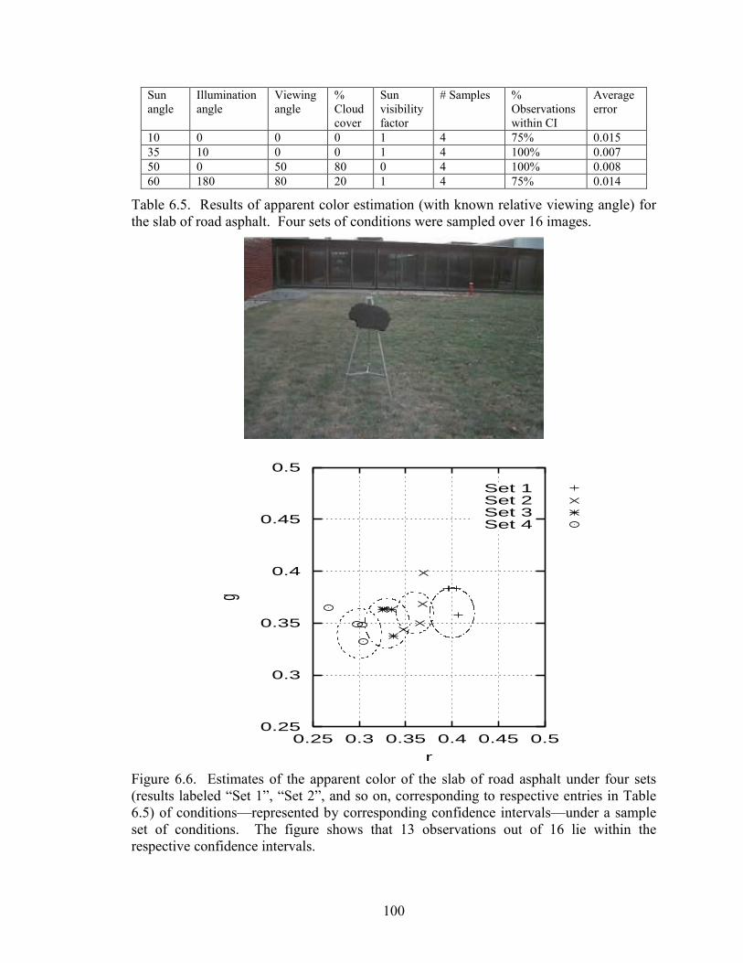
100

Sun angle

Illumination angle

Viewing angle

% Cloud cover



Average error

10 0 0 0 1 4 75% 0.015 35 10 0 0 1 4 100% 0.007 50 0 50 80 0 4 100% 0.008 60 180 80 20 1 4 75% 0.014

Table 6.5. Results of apparent color estimation (with known relative viewing angle) for the slab of road asphalt. Four sets of conditions were sampled over 16 images.

0.25

0.3

0.35

0.4

0.45

0.5

0.25 0.3 0.35 0.4 0.45 0.5

g

r


Figure 6.6. Estimates of the apparent color of the slab of road asphalt under four sets (results labeled “Set 1”, “Set 2”, and so on, corresponding to respective entries in Table 6.5) of conditions—represented by corresponding confidence intervals—under a sample set of conditions. The figure shows that 13 observations out of 16 lie within the respective confidence intervals.

101

6.3 Estimating apparent color when the viewing angle is unknown

The difference between estimating apparent color with and without knowledge of the

relative viewing angle is that the latter case has an uncertainty in the viewing angle of

180o. The apparent color is predicted to lie anywhere along the dichromatic line, leading

to less precise predictions. Note that the only surfaces to which the relative viewing

angle applies are those with a peaked NPF (i.e., specular surfaces with sunlight incident

upon them).

Just as Section 6.2.1 derived a noise model for estimating apparent color with known

relative viewing angle, the following discussion derives the noise model when the

relative viewing angle is not known. There are only two sources of noise in this method

of estimation: the error associated with the linear daylight function (Equation 4.3) and the

color-coefficient model. The error for the linear daylight function was discussed in the

previous section, and that for the coefficient model was determined in a test similar to

that used to derive the NPF error. When the two Gaussians are convolved, the composite

error model (for each surface) is a Gaussian centered about the dichromatic line for the

surface.

For the “No Parking” sign, the average error, measured as the perpendicular Cartesian

distance to the dichromatic line to the observed rgb point, was 0.006, and 18 out of 19

samples were within the confidence intervals which had an average area of about 0.0007

square units. For the “Stop” sign, the average error was 0.018, with 17 of 19 points being

within the confidence intervals which had an average area of about 0.006 square units.

When compared to the results when the viewing angle is known, the major difference is

that the confidence intervals tend to be larger when the viewing angle is not known,

102

because the estimate is a line segment instead of a point. Hence, even though error

margins appear similar, they are being measured differently: in the earlier case, the error

was being measured as a distance to a point; in this case the error is the perpendicular

distance to a line. Broader implications of this difference will become evident in the

following section, where image pixels are classified on the basis of the estimated

apparent color—larger confidence intervals will result in less accurate pixel

classification.

6.4 Pixel classification

After the apparent color is estimated for the specified conditions, image pixels can be

classified as either target or background. This section uses a classification method that is

based on the probability of a pixel being within the 2σ confidence interval of its estimated

apparent color. Classification results on the 90 images described in the following

sections for cases when the relative viewing angle is knows, and for those when it is not.

The classification results are evaluated in terms of two measures: the true positive rate

and the false positive rate. The true positive rate is the percentage of on-target pixels that

are correctly classified as targets, and the false positive rate represents the percentage of

background pixels that have been mis-classified as target.

6.4.1 Gaussian noise model for classification

The previous section discussed the noise models used for accounting for errors due to

the various empirical parameters. In order to determine the discriminant between target

and background pixels, this section examines Receiver-Operator Characteristic (ROC)

curves for each of the five target surfaces and the corresponding Gaussian distributions.

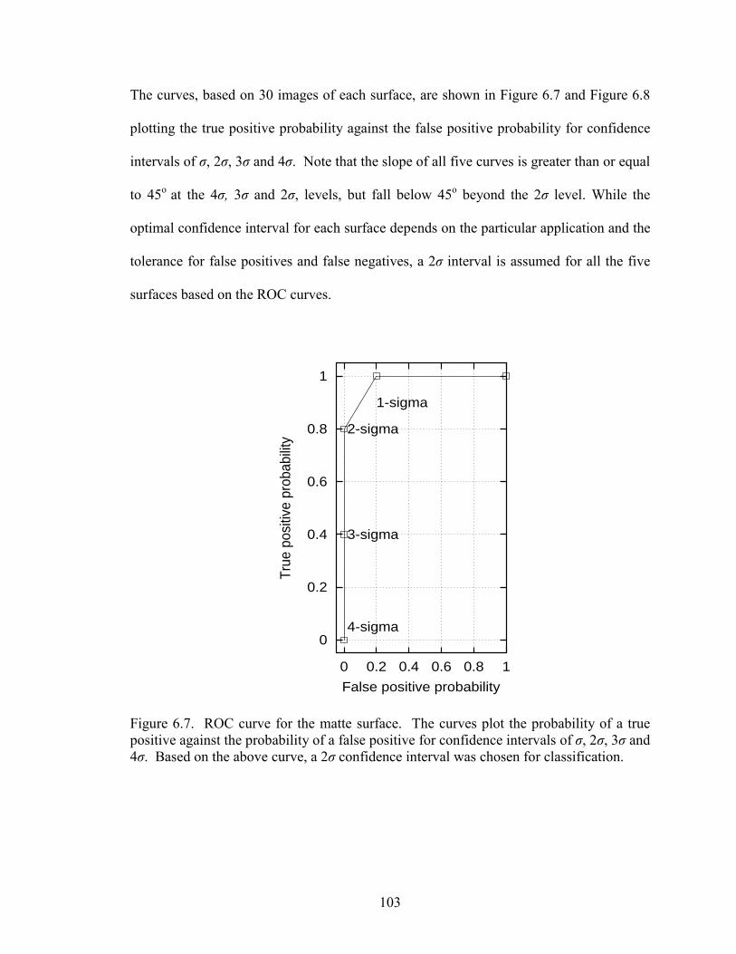
103

The curves, based on 30 images of each surface, are shown in Figure 6.7 and Figure 6.8

plotting the true positive probability against the false positive probability for confidence

intervals of σ, 2σ, 3σ and 4σ. Note that the slope of all five curves is greater than or equal

to 45o at the 4σ, 3σ and 2σ, levels, but fall below 45o beyond the 2σ level. While the

optimal confidence interval for each surface depends on the particular application and the

tolerance for false positives and false negatives, a 2σ interval is assumed for all the five

surfaces based on the ROC curves.

0

0.2

0.4

0.6

0.8

1

0 0.2 0.4 0.6 0.8 1

True

pos

itive

pro

babi

lity

False positive probability

3-sigma

2-sigma

1-sigma

4-sigma

Figure 6.7. ROC curve for the matte surface. The curves plot the probability of a true positive against the probability of a false positive for confidence intervals of σ, 2σ, 3σ and 4σ. Based on the above curve, a 2σ confidence interval was chosen for classification.

104

0

0.2

0.4

0.6

0.8

1

0 0.2 0.4 0.6 0.8 1

True

pos

itive

pro

babi

lity


3-sigma

2-sigma

1-sigma

4-sigma

0

0.2

0.4

0.6

0.8

1

0 0.2 0.4 0.6 0.8 1Tr

ue p

ositi

ve p

roba

bilit

y


3-sigma

2-sigma

1-sigma

4-sigma

(a) (b)

0

0.2

0.4

0.6

0.8

1

0 0.2 0.4 0.6 0.8 1

True

pos

itive

pro

babi

lity


3-sigma

2-sigma

1-sigma

4-sigma

0

0.2

0.4

0.6

0.8

1

0 0.2 0.4 0.6 0.8 1

True

pos

itive

pro

babi

lity


3-sigma

2-sigma

1-sigma

4-sigma

(c) (d) Figure 6.8. ROC curves for the (a) “Stop” sign, (b) “No Parking” sign, (c) concrete slab, and (d) road asphalt. The curves plot the probability of a true positive against the probability of a false positive for confidence intervals of σ, 2σ, 3σ and 4σ. Based on the above curves, a 2σ confidence interval was chosen for all four surfaces.

105

6.4.2 Brightness constraints

While the benefits of separating effects on brightness from those on normalized color

were discussed earlier in the context of the daylight and reflectance models, this section

develops a method for utilizing brightness as an additional constraint for classification

after the rgb color has been estimated. One of the disadvantages of using the rgb space is

that there is no distinction between surfaces with different brightness values but the same

normalized color. For example, in rgb, there is no difference between white, black and

all grays in between, even though a black (Lambertian) surface will never look white,31

and a white surface will not look black as long as there is a measurable amount of

incident light. Each point in rgb corresponds to a line in RGB, such that all the points on

the line have the same [R:G:B] ratio. Given that under a specific set of illumination and

viewing conditions, the apparent color of a surface is a point in RGB (rather than a line),

an rgb point classified as a target will also represent some points on the corresponding

RGB line that are not from targets. Since all the points along an RGB line collapse to a

single rgb point, these points cannot be differentiated in rgb, leading to false positives.

Hence, estimates of surface brightness are used as a constraint on the possible RGB

values of target pixels, after the initial classification in rgb. The constraints are based on

brightness values from Table 4.1, the Lambertian model, and more samples than are

required to derive the NPF. Note that the brightness constraint can be applied only when

the local surface orientation is known for the entire surface. While the orientation of a

planar surface may be a reasonable input parameter for this method, the entire map of

local surface normals for a non-planar surface is not. Hence, the brightness constraint 31 . . . unless the surface has a strong specular component and is illuminated by “white” light.

106

can be applied only to planar surfaces. In the case of non-planar surfaces, classification

is done in rgb, without the brightness constraint.32 The method is as follows:

1. The brightness entries from Table 4.1 are used, so as to include the mean and

standard deviation (VI and σVI, respectively) of the brightness of the incident light

under each set of conditions. It is assumed that changes in the brightness of the

white surface used for the deriving the daylight model are proportional to

corresponding changes in the brightness of the illuminant.

2. In Chapter 5, four samples were used to derive the NPF for the surface. The

modified procedure requires an additional 2 samples—one at a relative viewing

angle (n) of 0o and the other at one of the non-specular viewing angles (such as

30o). Both of these samples should be under illumination of different brightness

from the ones used for estimating the NPF. Hence, at each n, there is one pair of

samples of the target surface and a corresponding pair of samples of the white

surface. For the pair of samples at n = 0, if the brightness values of the target are

denoted by V0 and U0, and the corresponding values for the white surface denoted

by W0 and Y0, a brightness reflectance ratio (βs) for the specular component can be

defined as 0Y0W

0U0V

−

−. Similarly, from the samples at 30o, the brightness reflectance

ratio of the Lambertian component is estimated by βl = 30Y30W

30U30V

−

−. Please note that

the 7 samples used in our experiments represent the minimum required for the

model; while in general it is better to select a larger number of points, we used the

minimum required in order to demonstrate that the 7 samples are sufficient. 32 Although this section does not discuss results of classification for non-planar surfaces, Chapter 6 does.

107

3. The apparent target color is estimated in rgb for the given set of illumination and

viewing conditions, based on the method to be described above.

4. Under a given illuminant (with accompanying values of VI and σVI), the brightness

of the surface Vs is estimated by (Vs = VI × βs) if n = 0, and (Vs = VI × βl) if n is in

the non-specular range.

5. If the angle of incidence (i) is 0o, then no brightness falloff function is required,

because the brightness of the surface is at its maximum. For all other values of i,

the brightness is scaled by the Lambertian falloff function cos(i), resulting in the

expected apparent brightness of the surface, Va.

6. Based on the standard deviation of the illuminant brightness (σVI), the confidence

interval for Va is [Va–2σdβs, Va+2σdβs] for the specular range, and [Va–2σdβl,

Va+2σdβl] for the non-specular range.

6.4.3 Results: when the relative viewing angle is known

The above method was tested on the 90 images described earlier in Section 6.2, and

the following sections describe the detailed results for each surface. Overall, the average

true positives rates were 96.3%, 95.2%, 95.8%, 75.9% and 61.8%, for the matte paper,

the “No Parking” sign, the “Stop” sign, the concrete slab and the slab of asphalt,

respectively. The corresponding false positive rates were 1.2%, 3.6%, 4.4%, 12.1% and

20.8%. An analysis of the results pertaining to each surface follows.

108

6.4.3.1 Matte surface

Figure 6.9. Sample results of probability-based classification with a known viewing angle for the matte paper: the true and false positive rates were 96.3% and 1.2%, respectively.

109

Sun angle

Illumination angle

Viewing angle

% Cloud cover


# Samples True positive rate

False positive rate

10 0 0 0 1 5 96.5% 1.0% 35 10 0 0 1 4 97.0% 1.4% 50 0 50 80 0 6 96.1% 1.1% 60 180 80 20 1 5 97.4% 4.7%

Table 6.6. Results of probability-based classification for the matte paper, with known relative viewing angle. Four sets of conditions were sampled, with each row describing the sun angle, illumination angle, viewing angle, approximate cloud cover, and the sun visibility factor for the corresponding set of conditions. For each set of conditions, the number of samples are shown, along with the percentage of observations that fell within the estimated confidence interval, and the average error from the estimate.

For the matte surface, tests were conducted on 20 images over 4 sets of conditions

(Table 6.6). The true positive classification rate was about 96.3%, with a false positive

rate of 1.2% (see Figure 6.9 for a representative sample). The reason for the high true

positive classification rate is the low error in estimating the apparent color, and the fact

that the Cartesian distance between the observed rgb of the surface and that of the other

objects in the scene (0.01 for the grass, 0.82 for the leaves and 0.45 the surface in the

scene with the closest color) is well outside the 2σ confidence interval. In addition, the

surface is matte and its NPF is a straight line. This eliminates dependence on one

variable from the problem, namely the relative viewing angle, making the task of

estimation easier.

110

6.4.3.2 “No Parking” sign

Figure 6.10. Sample results of probability-based classification with a known viewing angle for the “No Parking” sign (specular case): the average true and false positive rates across all samples of the surface were 95.8% and 4.4%, respectively.

111

Sun angle

Illumination angle

Viewing angle

% Cloud cover


Effect # Samples

True positive rate

False positive rate

10 0 0 0 1 L 4 92.3% 4.1% 35 20 20 0 1 L 4 91.9% 3.8% 35 20 40 0 1 L 2 91.6% 3.2% 60 0 0 50 0.5 L 4 91.0% 3.6% 60 180 -30 20 1 L 5 92.1% 3.5% 10 0 0 0 1 S 4 97.4% 4.7% 35 20 20 0 1 S 4 90.4% 4.1% 60 0 0 50 0.5 S 4 97.0% 5.6% 10 0 0 0 1 T 4 94.3% 6.2% 35 20 20 0 1 T 4 96.2% 6.8% 60 0 0 50 0.5 T 4 95.3% 5.9%

Table 6.7. Results of probability-based classification for the “No Parking” sign—with known relative viewing angle—over five sets of conditions. Overall, 19 images were sampled out of which 12 exhibited Lambertian, specular and transition effects (shown as L, S and T in the 6th column); the remaining 7 samples exhibited only the Lambertian effect. Note that for the conditions which resulted in all three effects, the results for each effect are in a separate row.

For the “No Parking” sign, the “white” portion of the surface is the considered the

target and the lettering is considered background. In tests conducted on 19 images over 5

sets of conditions (Table 6.7), about 97.1% of the target pixels were detected, with a false

positive rate of about 5.1% (See Figure 6.10 and Figure 6.11 for sample results). The

“No Parking” sign has a strong specular component; hence, two cases arise, depending on

the surface orientation. In the first case, the relative viewing angle is in the specular

range (entries marked with “S” pixels in Table 6.7, and Figure 6.10). Because of

specular effect, almost the entire surface of the sign, including the lettering, is the color of

the illuminant. Hence, the target color is the color of the illuminant, which includes

pixels from all surfaces exhibiting the specular effect, as well as pixels on surfaces with a

neutral albedo (whites and grays). The high true positive classification rate was due to

the estimation accuracy. The results in Figure 6.10 also show small clusters of pixels

from background objects (e.g., to the left of the easel) that are classified as target pixels.

112

This is because these objects have neutral albedos and hence also reflect the color of the

illuminant. The 2σ confidence interval around the estimated rgb value of the target has a

small overlap with those for a few neutrally colored surfaces in the scene, thereby

causing the false positives. In the second scenario with the “No Parking” sign

(represented by the “L” pixel entries in Table 6.7, with a representative sample in Figure

6.11) a different set of phenomena occur. To begin with, because the relative viewing

angle is 20o, there is no specular effect, and the target area of the sign is the color of the

Lambertian component. Under those conditions about 91.2% of the pixels defined as

targets were within the confidence interval estimated rgb value, with a false positive rate

was about 3.6%. However, as Figure 6.11 shows, only about half of the actual sign is

classified as target. Specifically, there are two portions of the “No Parking” sign that are

classified as background: the lettering, and the pixels in the immediate neighborhood of

the lettering. The lettering, clearly, is background, and should be classified as such.

However, it is less obvious why the pixels neighboring the lettering are classified as

background. This occurs due to the mixed-pixel effect that is a consequence of the pixel

interpolation process that was discussed in Chapter 2. Because of the pixel interpolation,

the color of mixed pixels is somewhere in between the color of the lettering and that of

the target area. The mixed pixels were not considered part of the target; if they were, the

true positive rate would drop from 91.8% to 83.4% for the non-specular conditions. Even

without the specular effect, the albedo of the “No Parking” sign is almost neutral (i.e.,

white). As with the previous example, some pixels from background concrete and other

neutral colored objects are classified as targets.

113

Figure 6.11. Sample results of probability-based classification with a known viewing angle for the “No Parking” sign (non-specular case): the true and false positive rates were 95.8% and 4.4%, respectively.

114

6.4.3.3 “Stop” sign

Figure 6.12. Sample results of probability-based classification with a known viewing angle for the “Stop” sign: the true and false positive rates were 95.2% and 3.6%, respectively.

115

For the “Stop” sign, the “red” portion of the surface is considered the target area, and

the white lettering and border are considered background; as with the “No Parking” sign,

the “Stop” sign is also specular. In tests conducted on 19 images of the “Stop” sign,

about 95.8% of the target pixels were correctly classified, with a false positive rate of

about 4.4% (See Table 6.8). The false negatives occur because of two reasons: the first

is the mixed pixel effect described above, which accounts for about 20% of the false

negatives. The second reason is the classification method assumes that if one target pixel

in a given column is in the specular range, then all other target pixels in that column will

also be in the specular range (refer to Section 6.2.2); this assumption does not account for

the fact that the sun is (for all practical purposes) round, and hence the region on the

target representing the specular peak will be circular. This means that just as changes in

column numbers affects whether or not a pixel will be in the specular range, so will

changes in the row number; this phenomenon is not accounted for by the NPF-based

classifier. Most of the false positives, as in the case of the “No Parking” sign, occurred in

images with the specular effect, from areas with neutral albedos (such as concrete and the

white lettering and border). One noticeable phenomenon in the results for the “Stop”

sign from Figure 6.12 is that only the middle portion of the target surface reflects the

color of the illuminant, while the rest is the characteristic “red”. The “red” of the

Lambertian component was distinct in that there was no overlap between the confidence

interval around its estimated rgb; as a result, the true positive rate was high and the false

positive rate was low for that portion of the surface. At the same time, there were very

few neutral-colored or specular surfaces in the same range of columns as the specular

portion of the “Stop” sign, which also contributed to the low false positive rate.

116

However, there were some false negatives from the portion of the surface at the transition

between the regions representing the specular peak and the Lambertian component. This

was partially due to the mixed pixel effect.

Sun angle

Illumination angle

Viewing angle

% Cloud cover


Effect # Samples

True positive rate

False positive rate

10 0 0 0 1 L 5 94.5% 4.9% 35 30 30 0 1 L 3 93.8% 5.0% 35 20 40 0 1 L 2 96.7% 5.1% 60 0 0 50 0.5 L 4 95.2% 5.6% 60 180 -30 20 1 L 5 95.4% 4.7% 10 0 0 0 1 S 5 81.6% 8.4% 35 30 30 0 1 S 3 97.1% 4.2% 60 0 0 50 0.5 S 4 84.0% 5.1% 10 0 0 0 1 T 5 85.2% 4.8% 35 30 30 0 1 T 3 87.1% 5.2% 60 0 0 50 0.5 T 4 89.6% 4.9%

Table 6.8. Results of probability-based classification for the “Stop” sign—with known relative viewing angle—over five sets of conditions. Overall, 19 images were sampled out of which 12 exhibited Lambertian, specular and transition effects (shown as L, S and T in the 6th column); the remaining 7 samples exhibited only the Lambertian effect. Note that for the conditions which resulted in all three effects, the results for each effect are in a separate row.

117

6.4.3.4 Concrete slab

Figure 6.13. Sample results of probability-based classification with a known viewing angle for the concrete slab: the true and false positive rates were 75.9% and 12.1%, respectively.

118

The percentage of correctly classified pixels for the concrete slab was about 75.9%—

considerably lower than that for the matte surface and the traffic signs (See Figure 6.13

and Table 6.9). In addition, the false positive rate at the pixel level was higher: 12.1%.

The concrete slab in the figure is not uniformly colored, but has a vertical strip in the

middle that is a slightly different color, which explains the region in the middle classified

as non-target. One reason for the lower true positive classification rate is that the

concrete surface is not uniformly colored. It is a mixture of various substances such as

sand, crushed rocks and cement, and appears an even “gray” at a macro level (from a

distance). However a closer inspection shows that small portions of the concrete (at the

level of individual or small clusters of pixels in the image) have the color of the

constituent material used to form the concrete. This is because of the high standard

deviation of the average rgb color over the target area of the slab (which does not include

the vertical strip in the middle). The standard deviation was about three times that of the

matte surface and the traffic signs. The high standard deviation results in a higher

probability of classification error. At the same time, the confidence intervals for

estimated and observed rgb values of the target only partially overlapped. The concrete

slab was chosen because of its neutral “grayish” albedo, and the number of false positive

objects is due mostly to the presence of several other surfaces of neutral color. As in the

case of the traffic signs under the specular effect, color-neutrality makes detection

difficult because there are likely to be several neutrally colored surfaces in a typical

outdoor scene (such as concrete, pavement, road, etc.).

The examples of the traffic signs and the concrete surface illustrate another

phenomenon common to neutral colored surfaces and to surfaces with strong specular

119

components. This effect can be understood by imagining the rgb normalized dichromatic

lines for a number of surfaces, some specular and some neutral colored. All these lines

coincide at the illuminant point, making that part of the color space very ambiguous for

recognition. In other words, pixels in that part of color space could belong to any of a

number of (specular or neutral-colored) surfaces in the scene. Lee [46] describes a

number of examples such surfaces, along with their reflectances in normalized color

space.

Sun angle

Illumination angle

Viewing angle

% Cloud cover



False positive rate

10 0 0 0 1 4 84.0% 12.0% 35 10 0 0 1 4 76.1% 9.7% 50 0 50 80 0 4 68.5% 4.9% 60 180 80 20 1 4 76.2% 11.2%

Table 6.9. Results of probability-based classification for the concrete slab. Four sets of conditions were sampled over 16 images.

6.4.3.5 Road asphalt

Sun angle

Illumination angle

Viewing angle

% Cloud cover



False positive rate

10 0 0 0 1 4 54.8% 24.0% 35 10 0 0 1 4 62.1% 27.1% 50 0 50 80 0 4 71.1% 19.6% 60 180 80 20 1 4 62.4% 13.8%

Table 6.10. Results of probability-based classification for the slab of road asphalt. Four sets of conditions were sampled over 16 images.

The results from the slab of road asphalt were worse than those for the concrete

slab—only 61.8% of the target pixels were correctly classified, with a false positive rate

of 20.8% (See Table 6.10 and Figure 6.14). The reasons for the poor performance are

more extreme cases of the same factors affecting the concrete slab. To begin with, the

road surface is not uniformly colored, has the average rgb value is accompanied by a very

120

high standard deviation (0.012), leading to a larger confidence interval and consequently

higher classification errors, both in terms of false negatives and false positives. Second,

road asphalt is neutral colored, leading to a high false positive rate at the object level.

The examples of the road surface and the concrete slab show that for neutral colors, there

is so little color information that color may not be a good feature for recognition.

6.4.4 Results: when the relative viewing angle is not known

In the absence of knowledge about the relative viewing angle, the only surfaces

affected are those with a specular content, i.e., the traffic signs. As in Section 6.3, the

only difference is that classification is done based on the entire dichromatic line and the

corresponding confidence interval, rather than a point. For the “No Parking” sign, the

average true positive rate was about 95.3%, with an average false positive rate of about

7.4% (Figure 6.15). For the “Stop” sign, the corresponding rates were 97.1% and 10.8%,

respectively (Figure 6.16). Typically, the false positive rates will tend to be higher when

the viewing angle is not used, because targets are classified from a larger portion of the

color space. In addition, when the viewing angle is not known, the NPF cannot be used

to determine which target pixels will be specular and which non-specular; hence all

pixels are classified based on the dichromatic line, further increasing the likelihood of

false positives. However, the true positive rate should be at least as high, because the

target region in rgb does not get smaller.

The methods discussed in this section have been tested on images from two outdoor

applications: road/lane detection for automotive applications, and color-based focus-of-

attention for objects detection. These results are discussed in Chapter 7.

121

Figure 6.14. Sample results of probability-based classification with a known viewing angle for the slab of road asphalt: the true and false positive rates were 61.8% and 20.8%, respectively.

122

Figure 6.15. Results of probability-based classification without knowledge of the relative viewing angle for the “No Parking” sign.

123

Figure 6.16. Results of probability-based classification without knowledge of the relative viewing angle for the “Stop” sign.

124

7 APPLICATIONS CHAPTER 7

APPLICATIONS

7.1 Overview

This chapter discusses applications of the estimation and classification methods

developed in the previous sections. Section 7.2 describes a system for obstacle detection

for on-road automobiles, Section 7.3 discusses a method for detecting specific instances

of cars and similar objects in road scenes, and Section 7.4 examines the implications of

the results. The sections specifically describe the objective of each experiment, the

methodology and setup used, and the results/observations from the tests (including

measurement methodology).

7.2 On-road obstacle detection

As a part of the work leading to this dissertation, tests were conducted on data

collected in 1996-97 for developing color-based obstacle detection systems in the

National Automated Highway System (NAHS) project.

7.2.1 Objective

The goal of the experiments was to test the effectiveness of color-based pixel

classification in an obstacle detection system with the long-term goal of eventually

combining a suite of sensors and systems. The set of tests described were intended to test

how NPF-based classification would be able to recognize pixels that belonged to the road

surface and distinguish them from pixels from non-asphalt areas of the road (which are

presumably from potential obstacles). The system was biased towards being

125

conservative—i.e., avoiding false negatives at the risk of detecting more false positives or

false alarms—due to the nature of the application (obstacle detection for domestic

automobiles).

7.2.2 Methodology and setup

The method consisted of four steps: collecting the training data, collecting the test

data, classifying pixels, and using region-level logic with along with an external system

[74] to identify potential obstacles. To begin with, the surface reflectance parameters

were estimated from six randomly chosen training images (which, the reader may recall

from the discussion in Sections 5.4.1 and 6.4.2, is the minimum number of images

required to estimate the color-coefficient matrix and NPF). The data was collected using

the same Kodak digital camera used in the experiments in the previous sections; the

camera was mounted on the inside of a car on a fixed platform that was parallel to the

longitudinal axis of the car. The car was driven along a stretch of road on a test-track

belonging to an automobile manufacturing firm.33

The test data consisted of 5 sets of 25 images (for a total of 125) of a single stretch of

road, with the illumination conditions recorded. These five sets were collected over five

types of conditions (see Table 7.1): a clear morning (sun-angle 15o, cloud cover 0-5%), a

clear afternoon (sun-angle 45o, cloud cover 0-5%), a clear afternoon (sun-angle 50o,

cloud cover 0-5%), a cloudy evening (sun-angle 15o, cloud cover 60-70%, sun visibility

factor 0), and a cloudy morning (sun-angle 20o, cloud cover 60-70%, sun-visibility factor

0). The road surface in these images is locally horizontal with respect to the camera, so

that the viewing geometry is different for different parts of the road. However, since the

33 The firm wishes to remain anonymous.

126

road surface does not have a strong specular component (i.e., since it has a flat NPF), the

change in viewing geometry does not change the apparent color of the different parts of

the road. When the sun-visibility factor was non-zero (i.e., in the first, second and third

image sets), it was assumed that the light incident upon the surface was the color of

sunlight (as described in Table 4.1). Figure 7.1(a) shows a sample from the test set—as

the figure shows, the lane markers are clearly visible, and the lane is free of potholes.

What is less evident from the image is that there are occasional tire skid marks, oil

patches, and smudges from repeated painting of the right lane-marker. Four objects (a

car tire, a traffic cone, a cardboard box, and a nondescript piece of debris) were chosen as

obstacles and manually scattered over different, random parts of the road. Across the 125

images, there were 178 instances of obstacles. Figure 7.1(a) shows a single obstacle (the

nondescript piece of debris) about 60 feet in front of the car/camera.

Using the classification described in the previous chapter, the pixels in all 125 images

were classified into target and background classes. The output of this step is a set of

binary images. Figure 7.1(b) shows result from classifying the sample image in Figure

7.1(a). As the figure shows, there are a non-trivial number of false negatives as well as

false positives; details of the classification results will be discussed in the next section.

The logic used by the system was that any pixel that is not the color of the road is a

potential obstacle.

In order to detect obstacles at the region level, the lane-markers are first extracted

from the original color image using the intensity-profiling algorithm in the RALPH road-

follower [74]. Based on the lane-extraction, a triangular region is generated for the lane

occupied by the vehicle, stretching from the vanishing point to the part of the road just

127

before the vehicle. Note that for roads with curves, the RALPH algorithm “straightens”

the lanes by pixel-wise shifting of rows, so that the triangular region can still be fitted;

Figure 7.2(a) shows the triangular region extracted for the sample image. This process

considerably reduces the size of the search area, thereby voiding the impact of any errors

in color-based pixel classification outside the road area. Note also that pixels on the lane-

markers are themselves kept outside the triangle, removing them from the search

window. A 10×5 search window was used at the apex of the triangle, and any search

window with more that 10% (an empirically chosen number) non-road pixels was marked

as an obstacle. The size of the search window was gradually increased as the area being

searched approached the base of the triangle; the magnitude of the increase (15% per

iteration) was based on empirical measurements of loom (i.e., actual measurements of

how objects increased in size in the image as the approached the camera). Figure 7.2(b)

shows a sample result after extracting the obstacles using this technique—the obstacle is

detected, but so is one false positive. Evident in the figure is that most of the incorrectly

classified pixels within the search window did not result in errors at the region level

because of the size of the search window. However, the large number of positive pixels

near the bottom right corner of the search window (which were caused by minor

“smudging” of the lane marker during maintenance) caused the false positive shown in

the figure.

7.2.3 Results and observations

The performance of the system was evaluated at two levels: pixel level and region

level. At the pixel level, there are two measures of performance—the true positive rate

(which measures the percentage of non-road/obstacle pixels correctly identified), and the

128

false positive rate (which measures the percentage of road pixels identified as non-road).

Over the 125 images, the average estimation error (measuring the rgb distance between

with estimated and true colors under each set of conditions) was 0.013. The true and false

positive rates were determined by extracting road and non-road pixels from each image34

and counting the actual number of correctly and incorrectly classified pixels. The pixel-

level true positive rate was 76% (i.e., the false negative rate was 24%), with a 19% false

positive rate. Of the 24% false-negative pixels, a substantial number (about 90%) were

from the tire that was used as a sample obstacle (which is also black, the color of the

road). Out of the false positive pixels about 95% were from discolorations on the road

(specifically, oil patches, tire skid marks, road wear patches and shadows).

At the region level, the two measures of performance are the true positive rate

(number of full obstacles identified) and the false positive rate (number of full obstacles

missed). Note that the impact of pixel-level errors on region-level performance is

minimized by limiting the search area to the extracted triangle, and by applying loom-

based logic, which assumes that objects get larger as they approach the camera. Over the

125 images, 171 of the 178 obstacles were detected; the 7 obstacles that were undetected

were instances of the tire (which is the same color as the road). In addition, 107 regions

of the actual road were falsely identified as obstacles; these were all from the

discolorations due to tire skid-marks, road wear, shadows and oil. As mentioned earlier,

the high false positive number is the consequence of the conservative threshold (the

34 Pixels were extracted by drawing boxes (rectangular area provide a simple means for iterative region-extraction) around clusters of pixels and cropping them from the rest of the image. Because not all regions are rectangular (e.g., some obstacles are cones), only about 95% of the total pixels were actually evaluated.

129

reader may remember that any region with more that 10% non-road pixels is classified as

a potential obstacle).

Sun angle

% Cloud cover


Pixel true positive rate

Pixel false positive rate

Region true positive rate

# region false positives

15 0-5% 1 74% 17% 94% 20 45 0-5% 1 78% 19% 95% 23 50 0-5% 1 72% 16% 97% 24 15 60-70% 0 79% 20% 100% 19 20 60-70% 0 75% 21% 94% 21

Table 7.1. Results from NPF-based classification for road/obstacle detection. For each of the 5 test conditions, 25 images were sampled (for a total of 125 images). The table shows the true positive rate (76% overall) and false positive rate (19%) at the pixel-level for each set of conditions, along with the percentage of actual obstacles detected (96%, 171 out of 178) and the number false positives at the region-level (i.e., the number of times the obstacle detection system would have set off a false alarm, which occurred on the average 0.86 times per image).

130

(a) Original color image

(b) Classification for road pixels

Figure 7.1. Sample results from color-based classification used in conjunction with an external lane-extraction system: (a) original color image; (b) classification for road pixels.

131

(a) Lanes extracted using an external system

(b) Obstacle map

Figure 7.2. Sample results from color-based classification used with an external lane-extraction system: (a) triangular search regions after lane-extraction; (b) extracted obstacles: one true obstacle and one false positive.

132

7.3 Vehicle detection in road scenes

This section discusses the applicability of the NPF-based classifier in detecting

specific instances objects of known color (in this case, automobiles) in outdoor scenes.

7.3.1 Objective

In the following series of experiments, the goal was to determine the effectiveness of

the color estimation method for object identification, given the reflectance characteristics

(i.e., color and NPF) of the object’s surface. Such a system can be used for a number of

applications, such as searching through image databases (color-based image indexing),

traffic monitoring, etc. In this particular set of tests, the target objects were automobiles

(a car and a pickup truck), and the methods were used to identify instances of

automobiles with particular color characteristics (a dark shade of “red”).

7.3.2 Methodology and setup

As in the previous section, the experimental method consisted of four steps:

collecting the training data, collecting the test data, pixel classification, and using region-

level logic to identify potential obstacles. Surface reflectance parameters were estimated

from six randomly chosen training images of one specific automobile (the truck shown in

Figure 7.3(a)). The same Kodak digital camera from the earlier experiments was mounted

on a tripod with angular markings (in order to determine the exact illumination and

viewing angles). The target was defined as any instance of any automobile that is of the

particular shade of red (assuming that all such automobiles have similar specular

characteristics).35 In other words, the training data was obtained from a single vehicle,

35 This assumption might not hold for older automobiles with faded paint.

133

with the aim of detecting all vehicles in that have similar reflectance characteristics—the

reason being that even over a large set of images, only a small amount of training data

may be available. A total of 50 test images were collected, consisting of 10 images each

under 5 sets of conditions (see Table 7.2): a clear sky at 10o and 30o sun angles, and an

overcast sky at sun angles of 10o, 30o, and 50o (in dry and snowy conditions). All the

images were from the same parking lot over the course of 10 days; hence many of the

same automobiles were present in all the images. Figure 7.3 shows two of the sample test

images—in these images, there are two instances of potential target vehicle (shown in

ellipses). Across the 50 images, there were exactly 50 instances of 3 target automobiles.

In other words, there were only 3 red automobiles in the set of images, which collectively

appear 50 times in the 50 images (some images had more than one target, while some

others had none). The figure also shows that there is red-brick building in the

background, which looks very similar in color to the red vehicles. That background was

chosen intentionally, in order to test the effectiveness of the method in distinguishing

between subtle shades of the same general hue. In addition, the tail-lights of all the

vehicles shown in the figure are also of similar color.

As with the traffic signs discussed in the previous chapter, when direct sunlight is

incident upon the specular vehicle surface, a portion of the surface reflects the direct

sunlight, but the rest of the surface is still the characteristic “red” of the Lambertian

component. In order to deal with this problem, when the incident light was direct

sunlight and the relative viewing angle was 0o (for at least a portion of the target), both

the color of the sunlight and the apparent color of the Lambertian component were

134

considered target colors.36 In addition, since the surface of the vehicle is typically non-

planar, local surface brightness cannot be used; hence classification was done in the rgb

space. Figure 7.4 shows the binary images which resulted from classifying the images in

Figure 7.3. As the images show, a number of the pixels from the red-brick building and

car tail-lights were classified as targets (the next section will discuss the results in greater

detail).

After pixel classification, a standard boundary following algorithm [3] was used to

determine the (rectangular) size of pixel-clusters that were classified as target;

overlapping rectangular regions were coalesced together. Figure 7.5 shows the final

results on the two sample images.

7.3.3 Results and observations

For this test, all pixels on the body of the vehicles of the chosen vehicles—excluding

tires, mirrors and wind-shields—were considered target pixels. All other pixels,

including those from other the background building and tail-lights, were considered

background pixels. A false positive pixel was defined as any background pixel that was

classified as target, and any cluster of false positive pixels that was larger than 5×5 (this

size was empirically chosen to eliminate the effect of pixel-level noise) was considered a

false positive region.37 Any pixel on the body of the vehicle that was not classified as

target was considered a false negative (at the pixel level), and if there were no clusters on

the vehicle that were marked as targets, that failure was counted as one false negative at

36 The obvious risk with this assumption is that any specular surface can potentially be mis-classified as a target. For the purposes of this particular test, that risk was ignored. 37 This 5x5 window size was empirically chosen to eliminate the effect of pixel-level noise; as a result some small objects (e.g., tail-lights) were classified as false positives. In practice, the appropriate window size should be chosen depending on the false positive and false negative thresholds for the particular application.

135

the region level. Finally, multiple clusters on the body of vehicle were counted as one.

Over the 50 images, the average estimation error (measured as the distance between the

estimated and true rgb colors under each set of conditions) was 0.015, and the true

positive pixel classification rate was about 74% (i.e., with 26% false negatives), with a

false positive rate of about 11% (See Table 7.2 for more details). Further analysis of the

false negatives showed that about 80% of them due to light reflecting off other vehicles

in the proximity of the target; for instance, a green car next to the target would make the

specular surface of the target appear green rather than red. About 10% of the false

positives due to the deposition of snow on the body of the targets; the remaining were

simply outside the estimate confidence interval due to minor errors in the estimation. At

the region level, all 50 instances of the target were detected, along with 24 false positive

regions. As evident from the discussion of pixel-level false positives, all the false

negatives were from the red-brick building and the tail-lights.

7.4 Implications

The above results suggest that the NPF and daylight models provide an effective

platform for color-based pixel classification in unconstrained outdoor images. However,

the results also show that it is difficult to achieve true positive classification rates above

80%. This is primarily due to the confounding factors inherent in unconstrained outdoor

(e.g., inter-reflections, which are very difficult to model), suggesting that a significant

improvement in performance by adjusting the parameters of the daylight or NPF models

is not likely. However, utilization of region-level logic can prove to be a very effective

method of capitalizing on correct pixel-level results (which tend to occur in clusters)

while minimizing the impact of isolated pixel-level errors. In addition, the high rates of

136

region-level true and false positives highlight the benefit of combining a color-based

system with other sensor modalities (such as stereo-based systems [51] for separating

two-dimensional discolorations or patches on the road from three-dimensional objects)

for effective sensor fusion.

Sun angle

% Cloud cover


Pixel true positive rate

Pixel false positive rate

Region true positive rate

# region false positives

10 0-5% 1 74% 9% 100% 5 10 100% 0 70% 10% 100% 4 30 0-5% 1 76% 14% 100% 6 30 100% 0 71% 10% 100% 3 50 60-70% 0.5 79% 11% 100% 6

Table 7.2. Results from NPF-based classification for detection for specific instances of a characteristic (“red”) shade of automobile. For each of the 5 test conditions, 10 images were sampled (for a total of 50 images). The table shows the true positive rate (74% overall) and false positive rate (11%) at the pixel-level for each set of conditions, along with the percentage of actual instances detected (100%, 50 out of 50) and the number false positives at the region-level (24 separate instances, 0.48 instances per image).

137

Figure 7.3. Results of NPF-based classification for detecting a instances of automobiles of a characteristic (“red”) color: original images with targets marked (dark circles/ellipses).

138

Figure 7.4. Results of NPF-based classification for detecting a instances of automobiles of a characteristic (“red”) color: binary images resulting from pixel classification of the images shown in Figure 7.3.

139

Figure 7.5. Results of NPF-based classification for detecting a instances of automobiles of a characteristic (“red”) color: targets extracted (dark boxes) from the binary images shown in Figure 7.4.

140

8 CONCLUSIONS

CHAPTER 8

CONCLUSIONS

Of the contributions made in this dissertation, the most significant is a demonstration

of why a daylight model based on direct sampling of portions of the sky is not

appropriate for machine vision experiments. In particular, Chapter 4 shows that the CIE

radiometric model [42]—which has served as a standard of outdoor illumination—cannot

be directly used in machine vision to model light incident upon surfaces in an image.

The experiments in Chapter 4 show that this is primarily because the CIE data measures

light at the source (i.e., through direct measurements of sunlight and skylight), rather than

at the destination (i.e., the surface upon which the light is incident). Specifically, the

problems with the CIE data are (i) the small field-of-view sensors used for the CIE data

measure light from too small a portion of the sky, and (ii) measuring directly from the

source ignores the effect of light reflected off other surfaces in the scene, such as the

ground (thereby ignoring the significant amount of sunlight that can be reflected onto the

surface).

As a remedy, a model of daylight color is developed—this is the second contribution

of the study. The daylight model is in the form of a table that itemizes, for specific sky

conditions (sun angle, cloud cover, sun visibility factor), (i) the color of incident light

from the direction of the sun, (ii) the color of incident light from the direction away from

the sun, and (iii) the average color of skylight. The table also provides the standard

deviations and brightness values for each of these measurements in order to provide an

141

estimate of the expected consistency of the measurements. An additional (originally

unintended) application of the daylight table is in computer graphics models.

The third contribution of the study is a reflectance model (the Normalize Photometric

Function) that is a simplification of existing physics-based models [56][70][80] (that

cannot be used in outdoor color images) specifically for use in outdoor images. The

specific advantages of the NPF are that it (i) reliably models specularity for real surfaces

of different reflective characteristics, (ii) accounts for extended illumination (i.e.,

daylight, which is a combination of sunlight and ambient light), and (iii) eliminates the

dependence on brightness (which, as Chapter 4 shows, is extremely inconsistent and hard

to predict for incident daylight). Hence, the NPF maintains physics-based accuracy while

being simple enough to used in relatively unconstrained outdoor images.

The applicability of the daylight and NPF models to outdoor domains is demonstrated

over a large number of images. In the process of developing and testing the models, a

number of approximation methods for effectively dealing with the complexities of

outdoor images are also developed (such as the polyhedral model of omnidirectional

daylight, and the method for imposing brightness constraints in order to reduce false

positives).

This study is one of the first attempts at building usable models for color outdoor

machine vision. As a consequence, the robustness of the models across a broad range of

tests is yet to be proven. To begin with, the daylight model has been tested for three

relatively similar geographical locations in North America; it is not clear if the

consistency will hold in other parts of the world. Specifically, the effect of humidity,

haze and other particulate matter in the air may significantly affect the model. In

142

addition, the daylight model does not account for the effect of stray light from objects in

a complex scene (the simple polyhedral model notwithstanding); this may be a hindrance

to applying the model in unconstrained images.

The NPF model has proven to be a simple yet effective way of modeling reflectance

over a small set of surfaces. However, the tests over the concrete and asphalt slabs show

two weaknesses of this model. First, in neutral-colored surfaces, there may not be

enough color information for recognizing surfaces in normalized color space; hence, the

NPF may not provide as useful a description as an intensity-based model. Secondly, the

NPF is a local reflectance descriptor; as a consequence, surfaces that are not uniformly

colored cannot be easily modeled using such a method.

With the above in mind, potential future work is expected to be be along several

directions:

(i) Consolidating the daylight model to account for haze, humidity and other

atmospheric factors—this can either be in the form of additional entries

in the table, or as a parametric modification to existing entries based on

quantifiable measures of the above factors.

(ii) Testing the daylight model for robustness. Specifically, this will involve

(a) testing the consistency of the measurements across a broad range of

geographical areas, (b) testing robustness across different types of

cameras, and (c) building additional parameters (if required, in addition

to the polyhedral model) to account for the presence of multiple

reflective surfaces in the scene.

143

(iii) Testing the applicability of the NPF for surfaces that have characteristics

different from the ones tested. This could involve testing over a broad

range of Lambertian/specular characteristics, as well as uncommon

surfaces (e.g., fluorescent, retroreflective) surfaces that can occur in

outdoor domains.

(iv) Extending the NPF to model reflectance with non-uniform albedo.

Currently, the only way to deal with multicolored surfaces (e.g., the

traffic signs discussed in the earlier chapters) is to ignore the secondary

colors or model (and look for) one color at a time. A more elegant way

of dealing multi-colored surfaces will likely be very useful in building

real applications. This will be particularly useful for specular surfaces

which may exhibit both Lambertian and specular effects.

(v) Exploring new applications of the developed techniques.

144

APPENDICES

A.

APPENDIX A

RETROREFLECTIVITY

(a) Regular reflection (b) Retroreflection

Figure 9.1. Regular optical reflection vs. retroreflection: (a) In regular reflection, the reflected ray is symmetric to the incident ray across the surface normal; (b) In retroreflection, light is reflected back in the direction exactly opposite to the incident ray.

While retroreflectivity would ordinarily be out of the scope of a discussion of outdoor

color machine vision, it is discussed here because the experiments in the earlier chapters

use traffic signs. Many government-regulated traffic signs are designed to be

retroreflective, typically by mixing tiny beads of glass into the surface coating [1][89].

Retroreflectivity is a phenomenon in which light is reflected back along the direction of

illumination; this is done in order to enhance visibility of the signs to drivers at night,

when the illumination and viewing directions are assumed to be the same (i.e., the vehicle

carrying the driver). This phenomenon is different from regular optical reflection, in

which the reflected ray is symmetric to the incident ray across the surface normal. Figure

9.1 contrasts the two phenomena.

145

All that said, retroreflectivity is a non-issue in the experiments in this study because

the traffic signs used here were privately-owned and not retroreflective. Note, also, that

retroreflective surfaces are notorious for losing their property rapidly because of dirt and

exposure to the elements [1]; consequently, most traffic signs cease to be retroreflective a

few months (typically) after installation. Still, understanding how to address

retroreflectivity in the context of outdoor color machine vision may prove interesting;

hence a brief discussion follows.

Since retroreflectivity is a property specifically designed for night-time conditions

(i.e., a single beam of light in an otherwise dark setting), it is important to separate its

behavior at night from that under daylight. Under daylight, two further lighting

conditions exist: (a) when the surface faces away from the sun and is illuminated by

ambient skylight, and (b) when it is directly illuminated by sunlight. In the former case,

since the incident light is ambient, light is reflected back along all directions; in effect,

this result is exactly the same as regular, non-retroreflective refection.

Under direct sunlight, the process is only slightly more complicated. The reader may

recall that in Chapter 5, the relative viewing angle was defined as the difference between

the viewing angle and the angle of maximal reflectance. Since light is reflected back

along the illuminant direction in retroreflection, the angle of maximal reflectance is also

in the direction of incidence. Hence, the relative viewing angle is the angle between the

directions of viewing and incidence. The rest of the process of using the NPF, as

described in Chapter 5, is exactly the same as that for non-retroreflective surfaces.

The interpretation of the model under night conditions is similar to that under direct

sunlight—the relative viewing angle is still the angle between the directions of

146

illumination and viewing. The only difference is that under daylight, the presence of

ambient light makes the surface visible throughout the 180o field-of-view. Presumably,

the night-light is a non-ambient beam of light, which means that the surface is visible

from a much smaller range of viewing angles.

147

B. FLUORESCENCE

APPENDIX B

FLUORESCENCE

Fluorescence is the property that causes a surface to reflect light along a wavelength

that is longer than the incident light. The complication in modeling fluorescent

reflectance is that typically, a matrix specifying the complete spectra emitted as the result

of being exposed to a given wavelength is required [3]. Barnard [3] shows that it is

possible to model fluorescence based on some canonical illuminants. It may be possible

to use Barnard's method in place of the color-coefficient matrix to model the diffuse

component of surface reflectance under each of the entries in the daylight table, and then

apply the NPF to model specularity. However, since that line of research was considered

out of the scope of this particular study, it is not discussed further here; that said, it is one

potential subject of extensions to this study.

148

BIBLIOGRAPHY

[1] Anders, R. On-road investigation of fluorescent sign colors to improve conspicuity, Master of Science Thesis, Virginia Polytechnic Institute and State University, 2000.

[2] Arend, L. and Reeves, A. “Simultaneous color constancy”, Journal of the Optical

Society of America, 3(10):1743-1751, 1986.

[3] Ballard, D. and Brown, C. Computer Vision, Prentice-Hall, Englewood Cliffs, NJ, 1982.

[4] Barnard, K. “Color constancy with fluorescent surfaces”, Proceedings of the

IS\&T/SID Seventh Color Imaging Conference: Color Science, Systems and Applications, 1999.

[5] Boult, T. and Wolberg, G. “Correcting Chromatic Aberrations Using Image

Warping”, DARPA Image Understanding Workshop, 1992.

[6] Benzschawel, T., Brill, M. and Cohn, T. “Analysis of human color mechanisms using sinusoidal spectral power distributions”, Journal of the Optical Society of America, 3(10):1713-1725, 1986.

[7] Brainard, D. and Wandell, B. An Analysis of the Retinex Theory of Color Vision,

Stanford University Press, Stanford, CA, 1985.

[8] Buchsbaum, G. “A Spatial Processor Model for Object Colour Perception”, Journal of the Franklin Institute, 310:1-26, 1980.

[9] Budde, W. Unpublished, referenced in \cite.

[10] Buluswar, S. and Draper, B. “Color Recognition in Outdoor Images”, Proceedings of

the International Conference on Computer Vision, 1998.

[11] Buluswar, S. and Draper, B. “Nonparametric Classification of Pixels Under Varying Outdoor Illumination”, Proceedings of the DARPA Image Understanding Workshop, 1994.

[12] Chen, Y. and Hsu, Y. “Computer Vision on a Color-Blindness Plate”, Image and

Vision Computing, 13(6):463-478, August 1995.

[13] Cheng, F., Hsu, W. and Chen, T. “Recovering Colors in an Image with Chromatic Illuminant”, Image Processing, 7(11), November 1998.

[14] Condit, H. and Grum, F. “Spectral Energy Distribution of Daylight”, Journal of the

Optical Society of America, 54(7):937-944, 1964.

149

[15] Cook, R. and Torrance, K. “A Reflectance Model For Computer Graphics”, Image

Understanding, 2:1-19, 1987.

[16] Crisman, J. and Thorpe, C. “Color Vision for Road Following”, Vision and Navigation: The Carnegie Mellon NAVLAB, Kluwer, 1990.

[17] Dana, K., van Ginneken, B., Nayar, S. and Koenderink, J. “Reflectance and Texture

of Real World Surfaces”, ACM Transactions on Graphics, 18(1):1-34, 1999.

[18] Digital Video Cameras Co., On-line user information, http://www.edt.com/dvc/gamma.html.

[19] Dixon, E. “Spectral distribution of Australian daylight”, Journal of the Optical

Society of America, 68(4), July, 1964. [20] Finlayson, G. “Color Constancy in Diagonal Chromaticity Space”, Proceedings of the

Fifth International Conference on Computer Vision, 1995.

[21] Finlayson, G., Funt, B. and Barnard, K. “Color Constancy Under Varying Illumination”, Proceedings of the Fifth International Conference on Computer Vision, 1995.

[22] Finlayson, G.D., Drew, M.S. and Funt, B.V. “Diagonal Transforms Suffice”, Journal

of the Optical Society of America, 11(11):3011-3019, 1994.

[23] Finlayson, G., Hordley, S. and Hubel, P. “Color by Correlation: A Simple, Unifying Approach to Color Constancy”, Proceedings of the International Conference on Computer Vision, 1998.

[24] Forsyth, D. “A Novel Approach for Color Constancy”, International Journal of

Computer Vision, 5:5-36, 1990.

[25] Freeman, W. and Brainard, D. “Bayesian Decision Theory: the maximum local mass estimate”, Proceedings of the Fifth International Conference on Computer Vision, 1995.

[26] Funt, B. and Finlayson, G. “The State of Computational Color Constancy”,

Proceedings of the First Pan-Chromatic Conference, Inter-Society Color Council, 1995.

[27] Funt, B. and Drew, M. “Color Space Analysis of Mutual Illumination”, IEEE

Transactions on Pattern Analysis and Machine Intelligence, 12:1319-1326, 1993.

[28] Funt, B. and Finlayson, G. “Color constant color indexing” IEEE Transactions on Pattern Analysis and Machine Intelligence, 17(5):522-529, 1995.

150

[29] Funt, B., Barnard, K. and Martin, L. “Is Machine Color Constancy Good Enough?”, Proceedings of the Fifth European Conference on Computer Vision, 1998.

[30] Funt, B., Cardei, V. and Barnard, K. “Method of Estimating Chromaticity of

Illumination using Neural Networks” Proceedings of the IS\&T/SID Fourth Color Imaging Conference, 1996.

[31] Gershon, R., Jepson, A. and Tsotsos, J. The Effects of Ambient Illumination on the

Structure of Shadows in Chromatic Images. RBCV-TR-86-9, Dept. of Computer Science, University of Toronto, 1986.

[32] Grum, F. and Bartleson, C. Optical Radiation Measurements: Color Measurement,

Academic Press, 1980.

[33] Healy, G. “A Color Reflectance Model and its use for Segmentation”, International Conference on Computer Vision, 1988.

[34] von Helmholtz, H. Handbuch der Physiologischen Optik, Voss, Hamburg, 1896.

[35] Henderson, S. and Hodgkiss, D. “The Spectral Energy Distribution of Daylight”,

British Journal of Applied Physics, 14:125-131, 1963.

[36] Henry, R. “Colorimetry in the Natural Atmosphere”, Proceedings of the First Pan-Chromatic Conference, 1995.

[37] Hill, F. Computer Graphics, Macmillan, New York, 1990.

[38] Horn, B. Robot Vision, MIT Press, Cambridge, MA, 1987.

[39] Horn, B. “Understanding Image Intensities”, Artificial Intelligence, 8:201-231, 1977.

[40] Horowitz, P. and Hill, W. The Art of Electronics, Cambridge University Press,

Cambridge, UK, 1989

[41] Jackowski, M., Goshtasby, A., Bines, S., Roseman, D. and Yu, C. “Correcting the Geometry and Color of Digital Images”, IEEE Transactions on Pattern Analysis and Machine Intelligence, 19(10):1152-1158, October 1997.

[42] Judd, D., MacAdam, D. and Wyszecki, G. “Spectral Distribution of Typical Daylight

as a Function of Correlated Color Temperature”, Journal of the Optical Society of America, 54(8):1031-1040, 1964.

[43] Klinker, G., Shafer, S. and Kanade, T. “Color image analysis with an intrinsic

reflection model”, Proceedings of the International Conference on Computer Vision, 1988.

151

[44] von Kries, J. “Die Gesichtsempfindungen”, Handbuch Physiologie Menchen, 1904.

[45] Land, E. “Lightness and Retinex Theory”, Scientific American, 237(6):108-129, December 1977.

[46] Lee, H., Breneman, E. and Schulte, C. “Modeling light reflection for computer color

vision”, IEEE Transactions on Pattern Analysis and Machine Intelligence, 12:402-409, 1990.

[47] Lee, S. Understanding of Surface Reflections in Computer Vision by Color and

Multiple Views, Ph.D. Dissertation, University of Pennsylvania, 1992.

[48] Lenz, R., Osterberg, M., Hiltunen, J., Jaaskelainen, T. and Parkkinen, J. “Unsupervised filtering of color spectra,” Journal of the Optical Society of America, 13(7):1315-1324, 1996.

[49] Maloney, L. and Wandell, B. “Color Constancy: A Method for Recovering Surface

Spectral Reflectance”, Journal of the Optical Society of America, A3:29-33, 1986.

[50] Matloff, N. Probability Modeling and Computer Simulation, PWS-Kent, Boston, 1988.

[51] Matthies, L. “Stereo Vision for Planetary Rovers: Stochastic Modeling to Near Real-

Time Implementation”, International Journal of Computer Vision, 8(1):71-91, 1992.

[52] Maxwell, B. and Shafer, S. “A framework for segmentation using physical models of image formation”, IEEE Computer Society Conference on Computer Vision and Pattern Recognition, 1994.

[53] Meeus, J. Astronomical Formulae for Calculators, Willman-Bell, Richmond, 1985.

[54] Montag, J. “Influence of Boundary Information on the Perception of Color”, Journal

of the Optical Society of America-A, 14(5):997-1006, May 1997.

[55] Munsell Color (Corp.), Munsell Book of Color - Matte Finish Collection, Baltimore, MD, 1976.

[56] Nayar, S., Ikeuchi, K. and Kanade, T. “Determining Shape and Reflectance of Hybrid

Surfaces by Photometric Sampling”, IEEE Transactions on Robotics and Automation, 6:418-431, 1990.

[57] Nayar, S., Ikeuchi, K. and Kanade, T. “Surface Reflection: Physical and Geometric

Perspectives”, Carnegie Mellon University technical report, CMU-RI-TR-89-7, 1989.

[58] Nayatani, Y. and Wyszecki, G. “Color of Daylight from North Sky”, Journal of the Optical Society of America, 53(5):626-629, 1963.

152

[59] Nicodemus, F., Richmond, J., Hsia, J. Ginsberg, I. and Limperis, T. “Geometrical

considerations and nomenclature for reflectance”, NBS Monograph 160, National Bureau of Standards, 1977.

[60] Novak, C., Shafer, S. and Wilson, R. “Obtaining Accurate Color Images for Machine

Vision Research”, Proceedings of the SPIE, v 1250, 1990.

[61] Novak, C. and Shafer, S. A Method for Estimating Scene Parameters from Color Histograms, Carnegie Mellon University School of Computer Science, technical report, CMU-CS-93-177, 1993.

[62] Novak, L. and Hesse, S. “Optimal Polarizations for Radar Detection and Recognition

of Targets in Clutter”, Proceedings of the SPIE, 1992.

[63] Ohta, Y. and Hayashi, Y. “Recovery of Illuminant and Surface Colors from Images Based on the CIE Daylight”, Proceedings of the Third European Conference on Computer Vision, 1994.

[64] Ohta, Y. A region-oriented image-analysis system by computer, Doctoral

Dissertation, Kyoto University, Japan, 1980.

[65] Oren, M. and Nayar, S. “Generalization of the Lambertian Model and Implications for Machine Vision”, International Journal of Computer Vision, 14(3):227-251, 1995.

[66] Parkkinen, J. “Color Spectra Database”, Lappeenranta University of Technology on-

line data, http://www.lut.fi/ltkk/tite/research/color/lutcs_database.html.

[67] Parraga, C., Brelstaff, G., Troscianko, T. and Moorehead, I. “Color and Luminance Information in Natural Scenes”, Journal of the Optical Society of America-A, 15(3):563-569, March 1998.

[68] Petrov, A. “Surface Color and Color constancy”, Journal of Color Research and

Application, 18(4):236-240, 1993.

[69] Pietikaeinen, M., Nieminen, S., Marszalec, E. and Ojala, T. “Accurate Color Discrimination with Classification Based on Feature Distributions”, ICPR 91(2), 1996.

[70] Phong, B. “Illumination for Computer Generated Images”, Communications of the

ACM, 18:311-317.

[71] Plataniotis, K., Androutsos, D., Vinayagamoorthy, S., and Venetsanopoulos, A. “Color Image-Processing Using Adaptive Multichannel Filters”, Image Processing, 6(7):933-949, July 1997.

153

[72] Poggio, T. and Girosi, F. “Regularization algorithms for learning that are equivalent

to multilayer networks”, Science, 247:978-982, 1990.

[73] Pomerleau, D. Neural Network Perception for Mobile Robot Guidance, Kluwer Academic Publishers, Boston, 1993.

[74] Pomerleau, D. “RALPH: Rapidly Adapting Lateral Position Handler”, IEEE

Symposium on Intelligent Vehicles, 1995.

[75] Ripley, B. Pattern Recognition and Neural Networks, Cambridge University Press, 1996.

[76] Rogers, D. Procedural Elements for Computer Graphics, McGraw-Hill, New York,

1985.

[77] Sato, Y. and Ikeuchi, K. “Reflectance analysis under solar illumination”, Proceedings of the IEEE Workshop for Physics-based Modeling in Computer Vision, 1995.

[78] Sato Y. and Ikeuchi, K. “Temporal-color Space Analysis of Reflection”, Journal of

the Optical Society of America, 11(11):2990-3002,November, 1994.

[79] Schachter, B., Davis, L. and Rosenfeld, A. “Some Experiments in Image Segmentation by Clustering of Local Feature Values”, Pattern Recognition11(1):19-28, 1979.

[80] Shafer, S. “Using Color to Separate Reflection Components”, Color Research

Application, 10:210-218, 1985.

[81] Simonds, J. “Application of characteristic vector analysis to photographic and optical response data”, Journal of the Optical Society of America, 53(8), 1963.

[82] Swain, M. and Ballard, D. “Color Indexing”, International Journal of Computer

Vision, 7:11-32, 1991.

[83] Swain, M. “Happy patrons make better tippers: Creating a robot waiter using Perseus and the Animate Agent Architecture”, The 2nd International Conference on Automatic Face- and Gesture-Recognition, 1996.

[84] Syeda-Mahmood, T. “Detecting Perceptually Salient Texture Regions in Images”,

Computer Vision and Image Understanding, 76(1):93-108, October, 1999

[85] Syeda-Mahmood, T. and Cheng, Y. “Indexing Colored Surfaces in Images”, The Proceedings of the International Conference on Pattern Recognition, 1996.

154

[86] Thompson, E., Palacios, A. and Vareln, F. “Ways of coloring: Comparative color vision as a case study for cognitive science”, Behavioral Brain Sciences, 15, 1992.

[87] Torrance, K. and Sparrow, E. “Theory for Off-Specular Reflection from Roughened

Surfaces”, Journal of the Optical Society of America, 57:1105-1114, 1967.

[88] Trussell, H. and Kulkarni, M. “Sampling and Processing of Color Signals”, Image Processing, 5(4):677-681, April 1996.

[89] U.S. Department of Transportation, Federal Highway Administration, Manual on

uniform control devices, 2000. [90] Vrhel, M. and Trussell, H. “Filter considerations in color correction” IEEE

Transactions on Image Processing, 3:147-161, 1994.

[91] Vriesenga, M., Healey, G., Sklansky, J. and Peleg, K. Colored Illumination for Enhancing Discriminability in Machine Vision, Journal of Visual Communication and Image Representation, 6(3):244-255, September 1995.

[92] Wandell, B. Foundations of Vision, Sinauer Associates, Sunderland, MA, 1995.

[93] Wolff, L., Nayar, S. and Oren, M. “Improved Diffuse Reflection Models for

Computer Vision”, International Journal of Computer Vision, 30(1):55-71, 1998.

[94] Wyszecki, G. and Stiles, W. Color Science: Concepts and Methods, Quantitative Data and Formulas, John Wiley and Sons, Inc., New York, 1982.

[95] Yuille, A. “A method for computing spectral reflectance”, Biological Cybernetics,

56:195-201, 1987.

[96] Zaccarin, A. and Liu, B. “A Novel Approach For Coding Color Quantized Images”, Image Processing, 2(4):442-453, 1994.

[97] D'Zmura, M. and Iverson, G. “Color Constancy: Basic theory of two stage linear

recovery of spectral descriptions for lights and surfaces” Journal of the Optical Society of America, A 10:2148-2165, 1993.

[98] Zombeck, M. Handbook of Space Astronomy and Astrophysics, Cambridge

University Press, Cambridge, UK, 1990.

COLOR-BASED MODELS FOR OUTDOOR MACHINE VISION A ...

Documents

Transcript of COLOR-BASED MODELS FOR OUTDOOR MACHINE VISION A ...