Col Loch
28
1 | Page Control Electronic Summer In U B Training Report cs Optimization in FM-Atom Microscopes nternship (May 13 th to July 19 th 2013) Submitted by Gowtham Ragavendar G Undergraduate Student (Senior Yr) B. Tech – Engineering Physics IIT Delhi Under the guidance of Dr. Ashwin Lal Chief Technology Officer i2n Technologies Pvt. Ltd. Bangalore - 560012 mic Force
-
Upload
gowthamragav -
Category
Documents
-
view
25 -
download
2
description
v
Transcript of Col Loch
1 | P a g e
Control Electronics Optimization in FM
Summer Internship (May 13
Undergraduate Student (Senior Yr)
B. Tech
Training Report
Control Electronics Optimization in FM-Atomic Force
Microscopes
Summer Internship (May 13th to July 19
th 2013)
Submitted by
Gowtham Ragavendar G
Undergraduate Student (Senior Yr)
B. Tech – Engineering Physics
IIT Delhi
Under the guidance of
Dr. Ashwin Lal
Chief Technology Officer
i2n Technologies Pvt. Ltd.
Bangalore - 560012
Atomic Force
2 | P a g e
Contents Page
1. Introduction – Force Microscopy 3
2. Literature Survey 3
2.1 AFM Basics
2.1.1 Dynamic Mode of Operation 3
2.2 Components of FM-AFM 5
2.2.1 AFM Probe – Cantilever & Tip 5
2.2.2 Quartz Tuning Fork 5
2.2.3 Piezo Actuators 6
2.2.4 Control Electronics 6
3. FM-AFM system at i2n Technologies 8
4. Experimental Data Collection – Primary Data 10
5. Problem Definition 17
6. Modeling the Problem 17
6.1 Control Engineering – Mathematical Modelling 17
6.1.1 Open Loop and Closed Loop Control 18
6.1.2 Transfer Functions and Block Representation 18
6.2 PID Controller 19
7. Solution Methodology 20
7.1 Control Loop Simulation 20
7.2 Optimization Criteria 21
8. Conclusions 23
8.1 Simulink plot 23
9. Future Outlook 23
10. Appendix 24
10.1 Transfer Functions 24
10.2 Bode Plot & Nyquist Plot – MATLAB Simulink Tool 25
11. References 28
3 | P a g e
1. INTRODUCTION – Force Microscopy
Atomic Force Microscopy started in 1986 when the Atomic Force Microscope (AFM), was invented
by G. Binnig at Stanford University. Since then, a considerable number of improvements and
developments had been made, and many results had been achieved by simple contact
measurements. Nevertheless, contact AFM cannot generate true atomic resolution in a stable
operation. In 1995, non-contact AFM achieved true atomic resolution under attractive regime at
room temperature.
2. LITERATURE REVIEW
2.1 AFM Basics
The AFM consists of a cantilever with a sharp tip (probe) at its end that is used to scan the specimen
surface. The cantilever is typically silicon or silicon nitride with a tip radius of curvature on the
order of nanometers. When the tip is brought into proximity of a sample surface, forces between
the tip and the sample lead to a deflection of the cantilever according to Hooke's law. Typically, the
deflection is measured using a laser spot reflected from the top surface of the cantilever into an
array of photodiodes. Other methods that are used include optical interferometry, capacitive
sensing or piezoresistive AFM cantilevers. These cantilevers are fabricated with piezoresistive
elements that act as a strain gauge.
If the tip was scanned at a constant height, a risk would exist that the tip collides with the surface,
causing damage. Hence, in most cases a feedback mechanism is employed to adjust the tip-to-
sample distance to maintain a constant force between the tip and the sample. Traditionally, the
sample is mounted on a piezoelectric tube, which can move the sample in the z direction for
maintaining a constant force, and the x and y directions for scanning the sample. Alternatively a
'tripod' configuration of three piezo crystals may be employed, with each responsible for scanning in
the x,y and z directions. This eliminates some of the distortion effects seen with a tube scanner. In
newer designs, the tip is mounted on a vertical piezo scanner while the sample is being scanned in X
and Y using another piezo block. The resulting map of the area z = f(x,y) represents
the topography of the sample.
Noncontact AFM operates in static mode or dynamic mode, i.e., static AFM or dynamic AFM,
respectively. In static AFM the force Fts interacting between tip and sample translates into a
deflection of the cantilever, and the image is a map z(x, y, Fts) with Fts = constant.
2.2 Dynamic Mode of Operation
On the other hand, in dynamic AFM, the cantilever is deliberately vibrated. Dynamic mode imaging
is done using cantilevers of various frequency ranges Often as the cantilever resonant frequency
goes up, they get stiffer and have a higher Q. The higher Q provides greater amplitude amplification
of the drive signal and better frequency discrimination for small shifts due to surface interaction.
However, the extra stiffness of the cantilever might damage some materials, so there is a tradeoff to
be made on increasing the cantilever resonance.
4 | P a g e
The two basic methods are Amplitude Modulation (AM
AFM). In AM-AFM the cantilever is vibrated at a fixed frequency near the cantilever eigenfrequency.
The tip-sample interactions cause changes in both amplitude and phase, these changes are
measured and are used as the feedback signal. The speed of AM
factor of the cantilever, which slows the detection of surface features thr
effect in which a the tip goes off a cliff on the surface but doesn’t detect it for a while.
In FM-AFM the cantilever is also driven to oscillate at
In this mode, the change in the oscil
FM-AFM typically requires extremely high
The control signal is used to generate dissipation images. Another control loop is used to k
constant the cantilever’s oscillation frequency by adjustin
control signal is used to generate topographic images. Using FM
dramatically and for atomic studies in vacuum the FM is now t
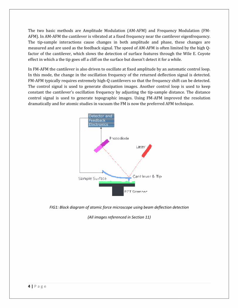
FIG1: Block diagram of atomic force microscope using beam deflection detection
(All images referenced in Section 11)
The two basic methods are Amplitude Modulation (AM-AFM) and Frequency Modulation (FM
AFM the cantilever is vibrated at a fixed frequency near the cantilever eigenfrequency.
sample interactions cause changes in both amplitude and phase, these changes are
measured and are used as the feedback signal. The speed of AM-AFM is often limited by the high Q
factor of the cantilever, which slows the detection of surface features through the Wile E. Coyote
effect in which a the tip goes off a cliff on the surface but doesn’t detect it for a while.
AFM the cantilever is also driven to oscillate at fixed amplitude by an automatic control loop.
change in the oscillation frequency of the returned deflection signal is detected.
extremely high-Q cantilevers so that the frequency shift
The control signal is used to generate dissipation images. Another control loop is used to k
ation frequency by adjusting the tip-sample distance
control signal is used to generate topographic images. Using FM-AFM improved the resolution
dramatically and for atomic studies in vacuum the FM is now the preferred AFM technique.
: Block diagram of atomic force microscope using beam deflection detection
(All images referenced in Section 11)
AFM) and Frequency Modulation (FM-
AFM the cantilever is vibrated at a fixed frequency near the cantilever eigenfrequency.
sample interactions cause changes in both amplitude and phase, these changes are
AFM is often limited by the high Q-
ough the Wile E. Coyote
effect in which a the tip goes off a cliff on the surface but doesn’t detect it for a while.
amplitude by an automatic control loop.
signal is detected.
Q cantilevers so that the frequency shift can be detected.
The control signal is used to generate dissipation images. Another control loop is used to keep
sample distance. The distance
AFM improved the resolution
he preferred AFM technique.
: Block diagram of atomic force microscope using beam deflection detection
5 | P a g e
2.3 Components of an AFM
2.3.1 AFM Probe – Cantilever & Tip
The AFM probe is a consumable and measuring device with a sharp tip on the free swinging end of
a cantilever which is protruding from a holder plate used in Atomic force microscopes (AFM). The
dimensions of the cantilever are in the scale of micrometers. The radius of the tip is in the scale of a
few nanometers. The holder plate, also called holder chip, - often 1.6 mm by 3.4 mm in size - allows
the operator to hold the AFM probe with tweezers and fit it into the corresponding holder clips on
the scanning head of the Atomic force microscope.
The tip material is generally chosen for specific properties of the surface it will interact
with. There are two basic designs of cantilevers. The most common is the thin rectangular
bar “diving board” shape, used in contact and AC mode operation.
However, there are other methods to excite vibrations in the FM-AFM which do not include
cantilevers with bending and torsional properties. The configuration currently in operation at i2n
does not feature rectangular diving board or triangular cantilevers, instead uses a tuning fork with
tip attached, which act as basis for both the actuator and sensor system.
2.3.2 Quartz Tuning Fork
One major approach for implementation of vibration in high resolution FM-AFM imaging, and
currently used in-house at i2n, is the use of quartz tuning-fork sensors (QTF).
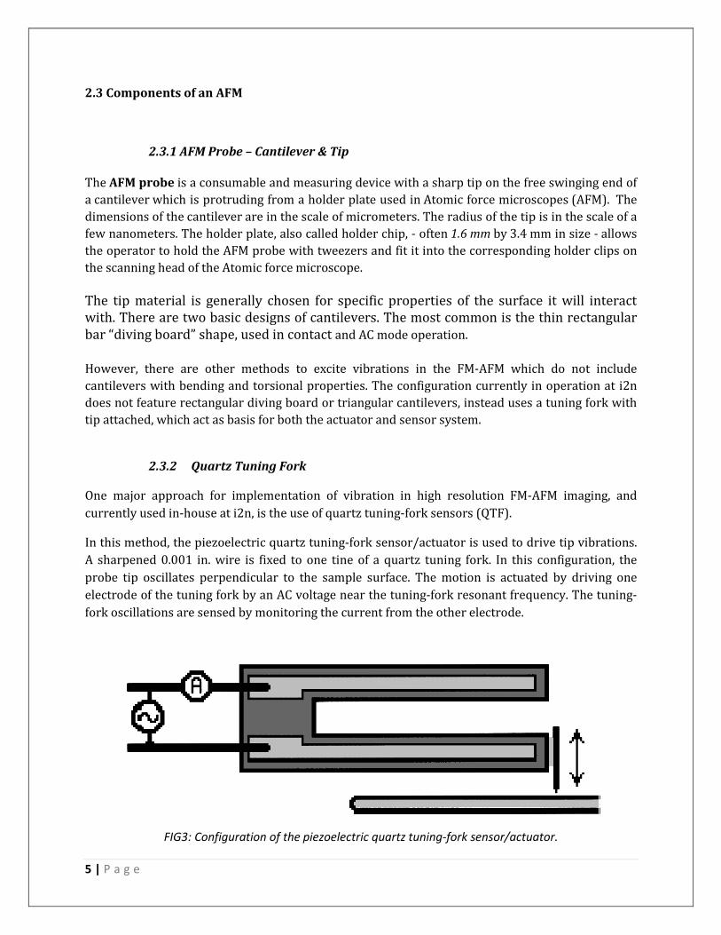
In this method, the piezoelectric quartz tuning-fork sensor/actuator is used to drive tip vibrations.
A sharpened 0.001 in. wire is fixed to one tine of a quartz tuning fork. In this configuration, the
probe tip oscillates perpendicular to the sample surface. The motion is actuated by driving one
electrode of the tuning fork by an AC voltage near the tuning-fork resonant frequency. The tuning-
fork oscillations are sensed by monitoring the current from the other electrode.
FIG3: Configuration of the piezoelectric quartz tuning-fork sensor/actuator.
6 | P a g e
The AFM tip is mounted perpendicular to the tuning-fork tine so that the tip oscillates normally to
the sample surface, minimizing tip wear. Furthermore, the high spring constant of the tuning-fork
allows the use of small oscillation amplitudes as small 0.1 nm, offering potentially improved spatial
resolution.
2.3.3 Piezo Actuators
A piezoelectric tube is a ceramic tube in which the many molecular dipoles are polarized at an
elevated temperature by applying a positive voltage to an outer electrode, causing the molecules to
partially align themselves with the positive directed outward. This results in + outer and - inner
radial polarization, which is made permanent by cooling. When subject to small voltages, the
element experiences a temporary expansion & contraction, leading to tube bending. This bending
action allows for piezo tubes to be used for XY-scanning in AFMs. However, this XY-direction
control is effected via the supporting software for the AFM usage, and not as a part of the PID
control apparatus, and thus it will remain outside the scope of further analysis, in this report.
2.3.4 Control Electronics
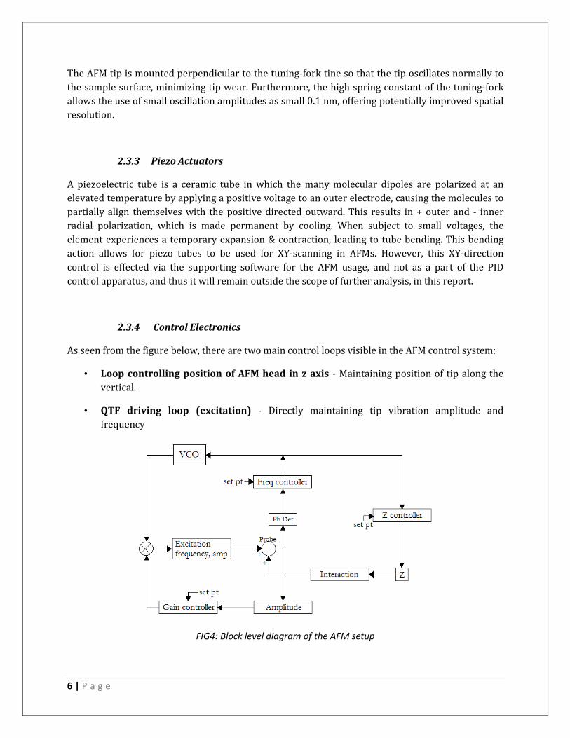
As seen from the figure below, there are two main control loops visible in the AFM control system:
• Loop controlling position of AFM head in z axis - Maintaining position of tip along the
vertical.
• QTF driving loop (excitation) - Directly maintaining tip vibration amplitude and
frequency
FIG4: Block level diagram of the AFM setup
7 | P a g e
Due to the high mechanical Q of quartz tuning forks, there is a delay of tens to hundreds of ms
before the tuning-fork oscillations reach their steady-state condition. As a result, traditional, ‘‘open-
loop,’’ methods of AFM are not appropriate for tuning-fork feedback. Since an AFM could not track a
surface at a scan rate faster than 0.1 Hz with a 100 ms lag in its sensor, we use a phase-locked-loop
(PLL) circuit to overcome this limitation by actively tracking the tuning-fork resonant frequency.
A Phase Locked Loop (PLL) present inside the VCO (Voltage Controlled Oscillator) performs the
function of frequency control. A phase-locked loop or phase lock loop (PLL) is a control system that
tries to generate an output signal whose phase is related to the phase of the input "reference"
signal. This circuit compares the phase of the input signal with the phase of the signal derived from
its output oscillator and adjusts the frequency of its oscillator to keep the phases matched. The
signal from the phase detector is used to control the oscillator in a feedback loop.
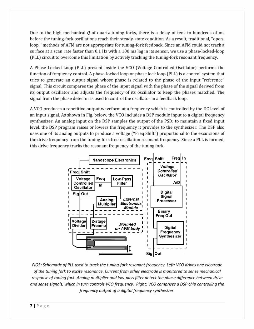
A VCO produces a repetitive output waveform at a frequency which is controlled by the DC level of
an input signal. As shown in Fig. below, the VCO includes a DSP module input to a digital frequency
synthesizer. An analog input on the DSP samples the output of the PSD; to maintain a fixed input
level, the DSP program raises or lowers the frequency it provides to the synthesizer. The DSP also
uses one of its analog outputs to produce a voltage (‘‘Freq Shift’’) proportional to the excursions of
the drive frequency from the tuning-fork free-oscillation resonant frequency. Since a PLL is formed,
this drive frequency tracks the resonant frequency of the tuning fork.
FIG5: Schematic of PLL used to track the tuning-fork resonant frequency. Left: VCO drives one electrode
of the tuning fork to excite resonance. Current from other electrode is monitored to sense mechanical
response of tuning fork. Analog multiplier and low-pass filter detect the phase difference between drive
and sense signals, which in turn controls VCO frequency. Right: VCO comprises a DSP chip controlling the
frequency output of a digital frequency synthesizer.
8 | P a g e
3. FM-AFM SYSTEM AT i2n TECHNOLOGIES
The two control loops in the diagram FIG4 are independent loops which have output values which
together contribute towards the input of the QTF probe. The Frequency controller and Gain
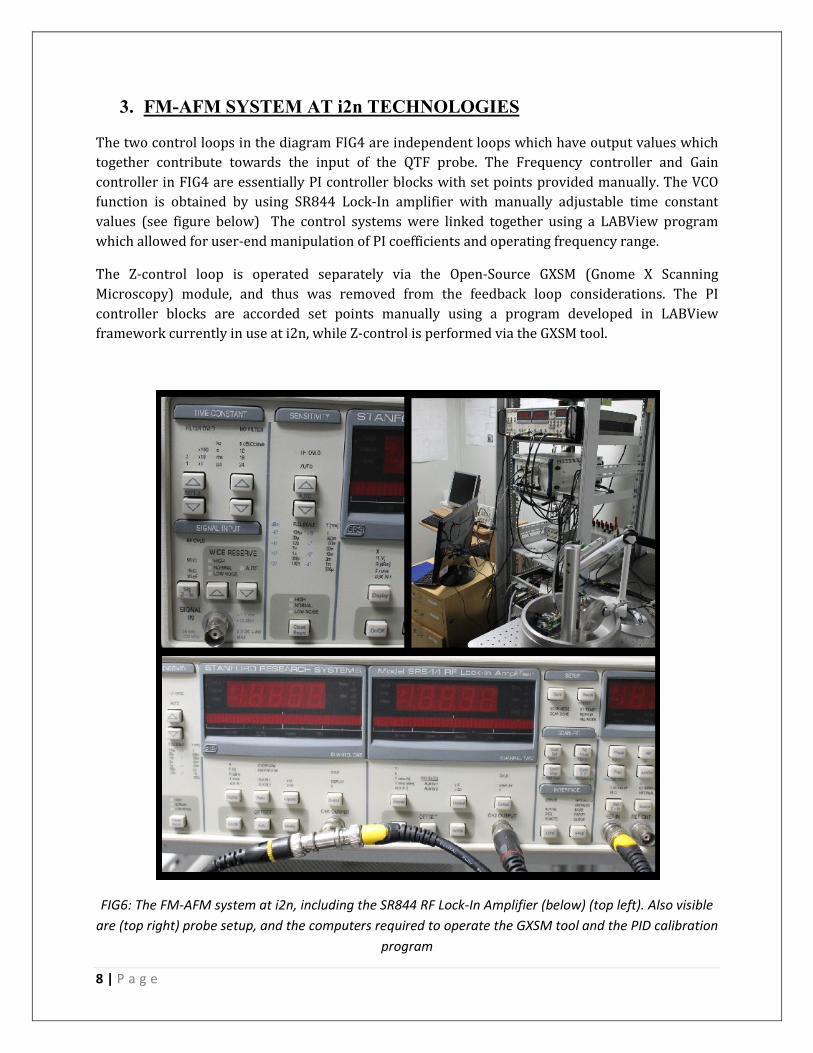
controller in FIG4 are essentially PI controller blocks with set points provided manually. The VCO
function is obtained by using SR844 Lock-In amplifier with manually adjustable time constant
values (see figure below) The control systems were linked together using a LABView program
which allowed for user-end manipulation of PI coefficients and operating frequency range.
The Z-control loop is operated separately via the Open-Source GXSM (Gnome X Scanning
Microscopy) module, and thus was removed from the feedback loop considerations. The PI
controller blocks are accorded set points manually using a program developed in LABView
framework currently in use at i2n, while Z-control is performed via the GXSM tool.
FIG6: The FM-AFM system at i2n, including the SR844 RF Lock-In Amplifier (below) (top left). Also visible
are (top right) probe setup, and the computers required to operate the GXSM tool and the PID calibration
program
9 | P a g e
4. EXPERIMENTAL DATA COLLECTION: Operating the AFM
In the second phase of the internship, the learnings from the literature review was put to
experiment by operating the FM-AFM in the premises of i2n. This allowed for a weeklong
immersion in the functioning controls of the running software used, and the best-practices and
safety precautions required to be adopted by user while operating the AFM.
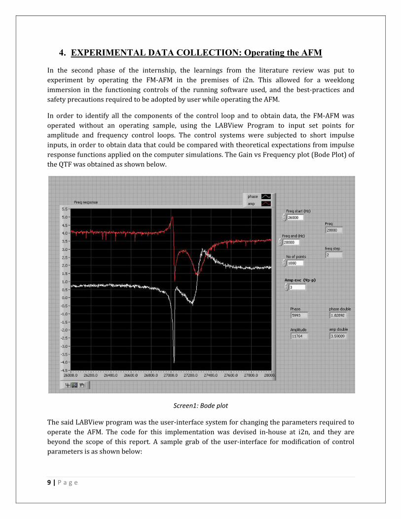
In order to identify all the components of the control loop and to obtain data, the FM-AFM was
operated without an operating sample, using the LABView Program to input set points for
amplitude and frequency control loops. The control systems were subjected to short impulse
inputs, in order to obtain data that could be compared with theoretical expectations from impulse
response functions applied on the computer simulations. The Gain vs Frequency plot (Bode Plot) of
the QTF was obtained as shown below.
Screen1: Bode plot
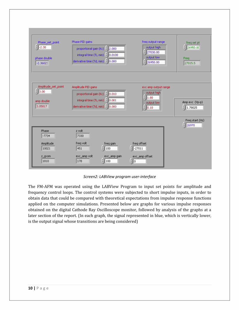
The said LABView program was the user-interface system for changing the parameters required to
operate the AFM. The code for this implementation was devised in-house at i2n, and they are
beyond the scope of this report. A sample grab of the user-interface for modification of control
parameters is as shown below:
10 | P a g e
Screen2: LABView program user-interface
The FM-AFM was operated using the LABView Program to input set points for amplitude and
frequency control loops. The control systems were subjected to short impulse inputs, in order to
obtain data that could be compared with theoretical expectations from impulse response functions
applied on the computer simulations. Presented below are graphs for various impulse responses
obtained on the digital Cathode Ray Oscilloscope monitor, followed by analysis of the graphs at a
later section of the report. (In each graph, the signal represented in blue, which is vertically lower,
is the output signal whose transitions are being considered)
11 | P a g e
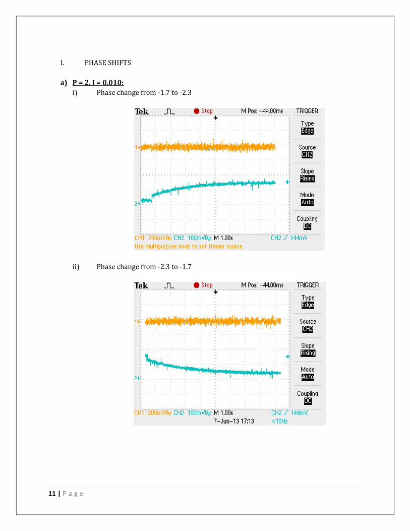
I. PHASE SHIFTS
a) P = 2, I = 0.010:
i) Phase change from -1.7 to -2.3
ii) Phase change from -2.3 to -1.7
12 | P a g e
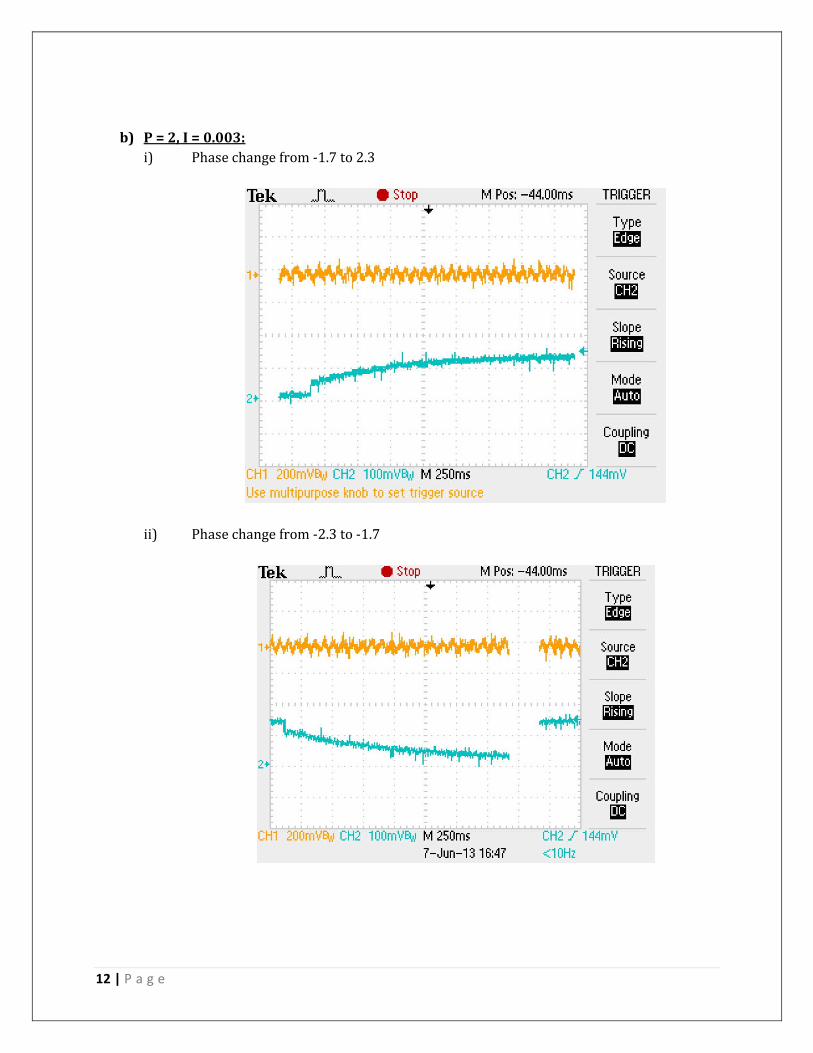
b) P = 2, I = 0.003:
i) Phase change from -1.7 to 2.3
ii) Phase change from -2.3 to -1.7
13 | P a g e
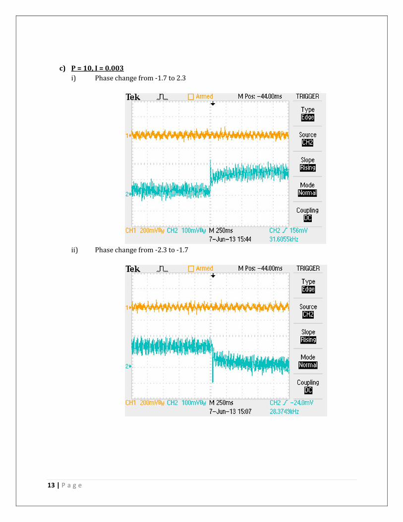
c) P = 10, I = 0.003
i) Phase change from -1.7 to 2.3
ii) Phase change from -2.3 to -1.7
14 | P a g e
II. AMPLITUDE SHIFTS
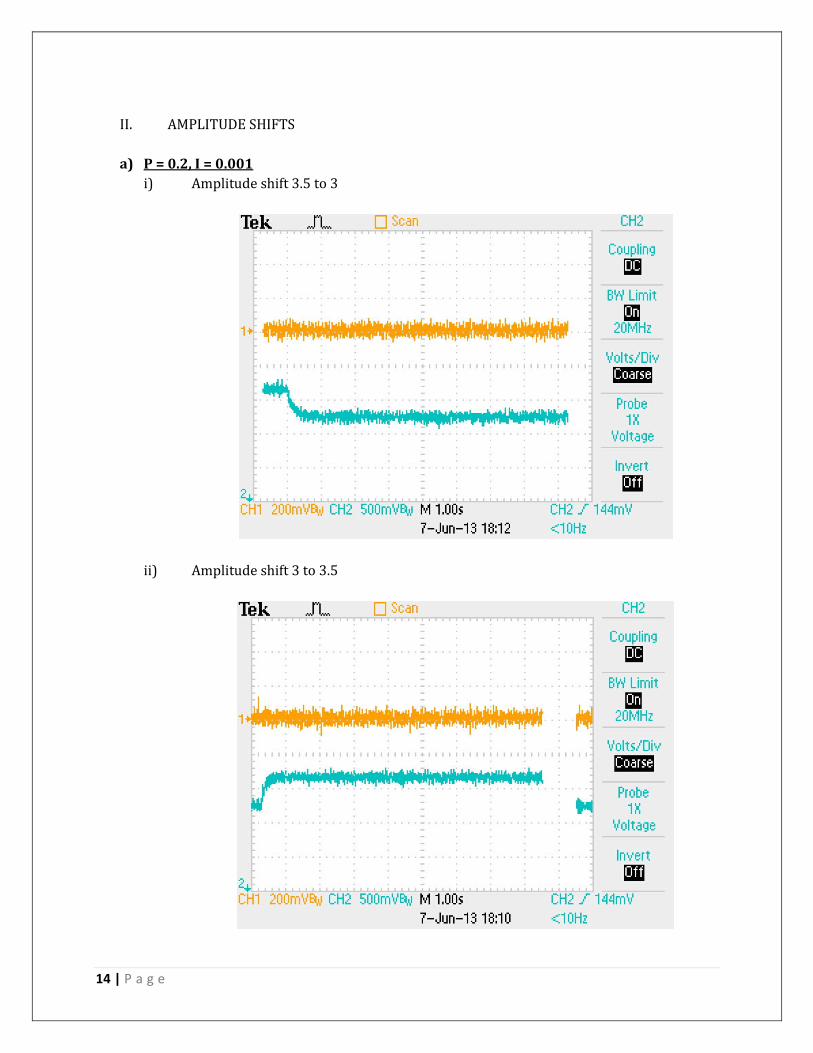
a) P = 0.2, I = 0.001
i) Amplitude shift 3.5 to 3
ii) Amplitude shift 3 to 3.5
15 | P a g e
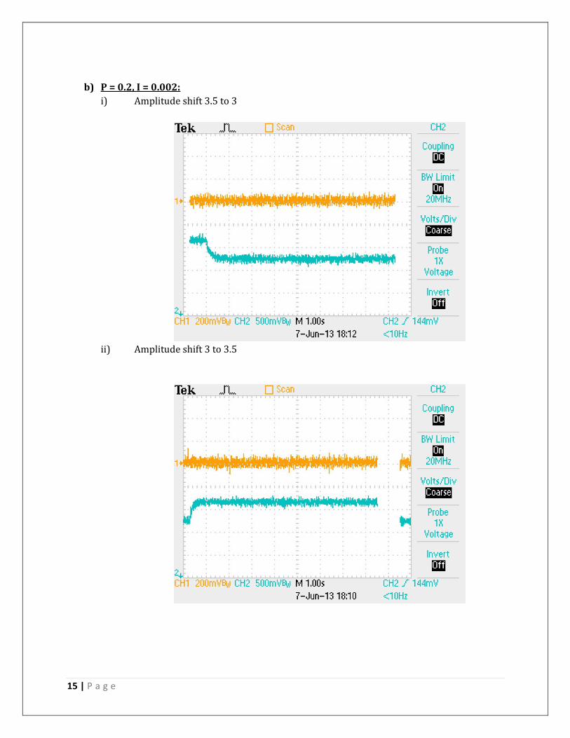
b) P = 0.2, I = 0.002:
i) Amplitude shift 3.5 to 3
ii) Amplitude shift 3 to 3.5
16 | P a g e
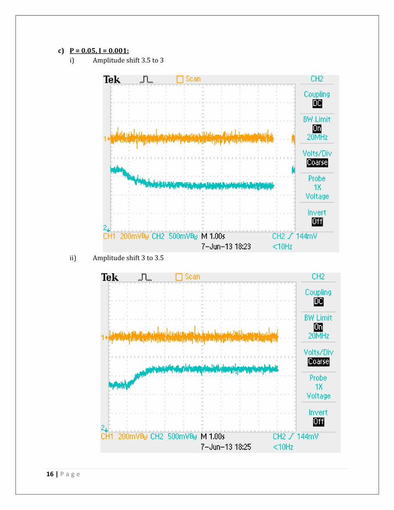
c) P = 0.05, I = 0.001:
i) Amplitude shift 3.5 to 3
ii) Amplitude shift 3 to 3.5
17 | P a g e
5. PROBLEM DEFINITION
For operating the FM-AFM to obtain high-resolution images at the nano level, the question at hand
is the selection of proper values as PI controller coefficients. The values of these coefficients are
to be selected optimally in order to avoid control loop instability, contact between tip and sample,
wear-and-tear of the tip and improper scanning of the surface. At i2n Technologies, the prevalent
procedure for arriving at optimum PI constants was via trial-and-error. This would require
considerable time and effort as preparation and calibration, and the set-up the FM-AFM would
become a tedious process. A need was felt to understand the basics of optimum constants in the
control loop in order to automate their selection. Thus, the project was aimed at identifying the
constraints responsible for selection of optimum PI coefficients and achieving critical damping
conditions inside the FM-AFM control loop.
6. MODELLING THE PROBLEM
Optimizing the PI controller to identify suitable constants required a thorough understanding the
basics of control engineering. Provided below is a brief review of the basic concepts on control
systems, which form the basis for understanding in subsequent sections of this report.
6.1 Control Engineering: Mathematical Modeling
6.1.1 Open-Loop and Closed-Loop Controller
An open-loop controller is a type of controller that computes its input into a system using only the
current state and its model of the system.
A characteristic of the open-loop controller is that it does not use any signal from its output to
determine if its output has achieved the desired goal of the input. This means that the system does
not observe the output of the processes that it is controlling. Consequently, a true open-loop system
can not engage in machine learning and also cannot correct any errors that it could make. It also
may not compensate for disturbances in the system.
To overcome these limitations of the open-loop controller, control theory introduces feedback. A
closed-loop controller uses feedback to control states or outputs of a dynamical system. Its name
comes from the information path in the system: process inputs (e.g., voltage applied to an electric
motor) have an effect on the process outputs (e.g., speed or torque of the motor), which is
measured with sensors and processed by the controller; the result (the control signal) is "fed back"
as input to the process, closing the loop.
18 | P a g e
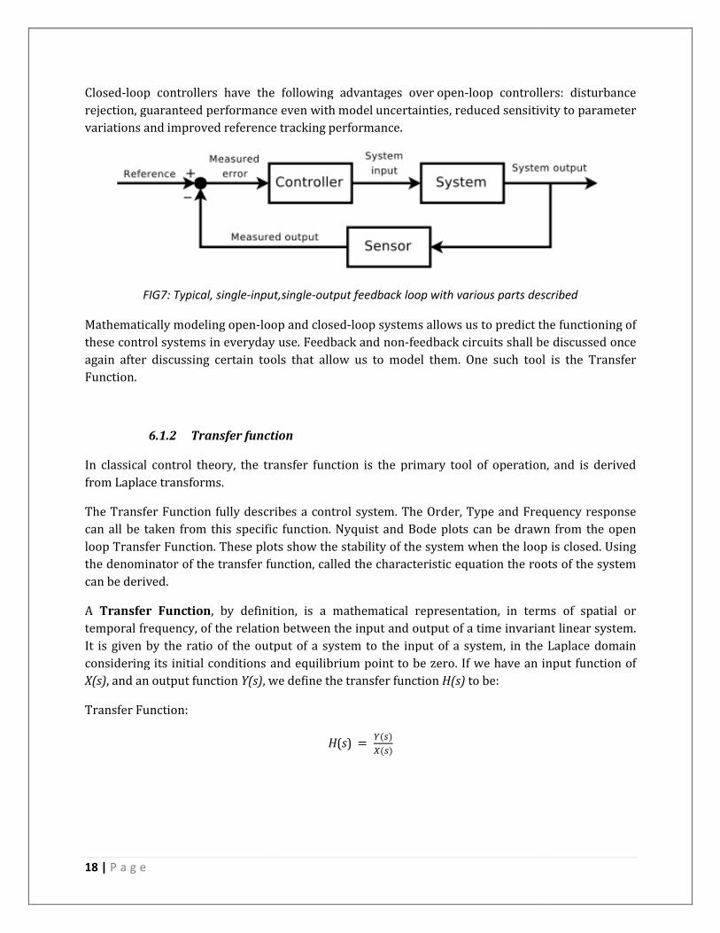
Closed-loop controllers have the following advantages over
rejection, guaranteed performance even with
variations and improved reference tracking performance
FIG7: Typical, single-input,single
Mathematically modeling open-loop and closed
these control systems in everyday use. Feedback and non
again after discussing certain tools that allow us to model them. One such
Function.
6.1.2 Transfer function
In classical control theory, the transfer function is the primary tool of operation, and is derived
from Laplace transforms.
The Transfer Function fully describes a control system. The Order, Type and Frequ
can all be taken from this specific function. Nyquist and Bode plots can be drawn
loop Transfer Function. These plots show the stability of the system when
the denominator of the transfer function,
can be derived.
A Transfer Function, by definition, i
temporal frequency, of the relation between the input and output of a
It is given by the ratio of the output of a system to the input of a system, in
considering its initial conditions and equilibrium point to be zero. If we
X(s), and an output function Y(s), we define
Transfer Function:
loop controllers have the following advantages over open-loop controllers:
guaranteed performance even with model uncertainties, reduced sensitivity to parameter
improved reference tracking performance.
input,single-output feedback loop with various parts described
loop and closed-loop systems allows us to predict the functioning of
these control systems in everyday use. Feedback and non-feedback circuits shall be discussed once
again after discussing certain tools that allow us to model them. One such tool is the Transfer
Transfer function
theory, the transfer function is the primary tool of operation, and is derived
The Transfer Function fully describes a control system. The Order, Type and Frequ
can all be taken from this specific function. Nyquist and Bode plots can be drawn
loop Transfer Function. These plots show the stability of the system when the loop is closed. Using
the denominator of the transfer function, called the characteristic equation the roots of the system
, by definition, is a mathematical representation, in terms of spatial or
temporal frequency, of the relation between the input and output of a time invariant lin
of the output of a system to the input of a system, in the Laplace domain
considering its initial conditions and equilibrium point to be zero. If we have an input function of
, we define the transfer function H(s) to be:
H(s) � ��������
loop controllers: disturbance
reduced sensitivity to parameter
output feedback loop with various parts described
loop systems allows us to predict the functioning of
feedback circuits shall be discussed once
tool is the Transfer
theory, the transfer function is the primary tool of operation, and is derived
The Transfer Function fully describes a control system. The Order, Type and Frequency response
can all be taken from this specific function. Nyquist and Bode plots can be drawn from the open
the loop is closed. Using
equation the roots of the system
s a mathematical representation, in terms of spatial or
time invariant linear system.
the Laplace domain
have an input function of
19 | P a g e
6.1.3 PID Controller
PID controllers are combinations of the proportional, derivative, and integral controllers:
Proportional controllers are simply gain values. These are essentially multiplicative coefficients,
usually denoted with a K.
Derivative controllers can be shown using Laplace calculus in simplified forms. In the Laplace
domain, we can show the derivative of a signal using the following notation: D(s) = L{ f’(t) } = sF(s)
The derivative controllers are implemented to account for future values, by taking the derivative,
and controlling based on where the signal is going to be in the future. Thus, even small amount of
high-frequency noise can cause very large derivatives, which appear like amplified noise.
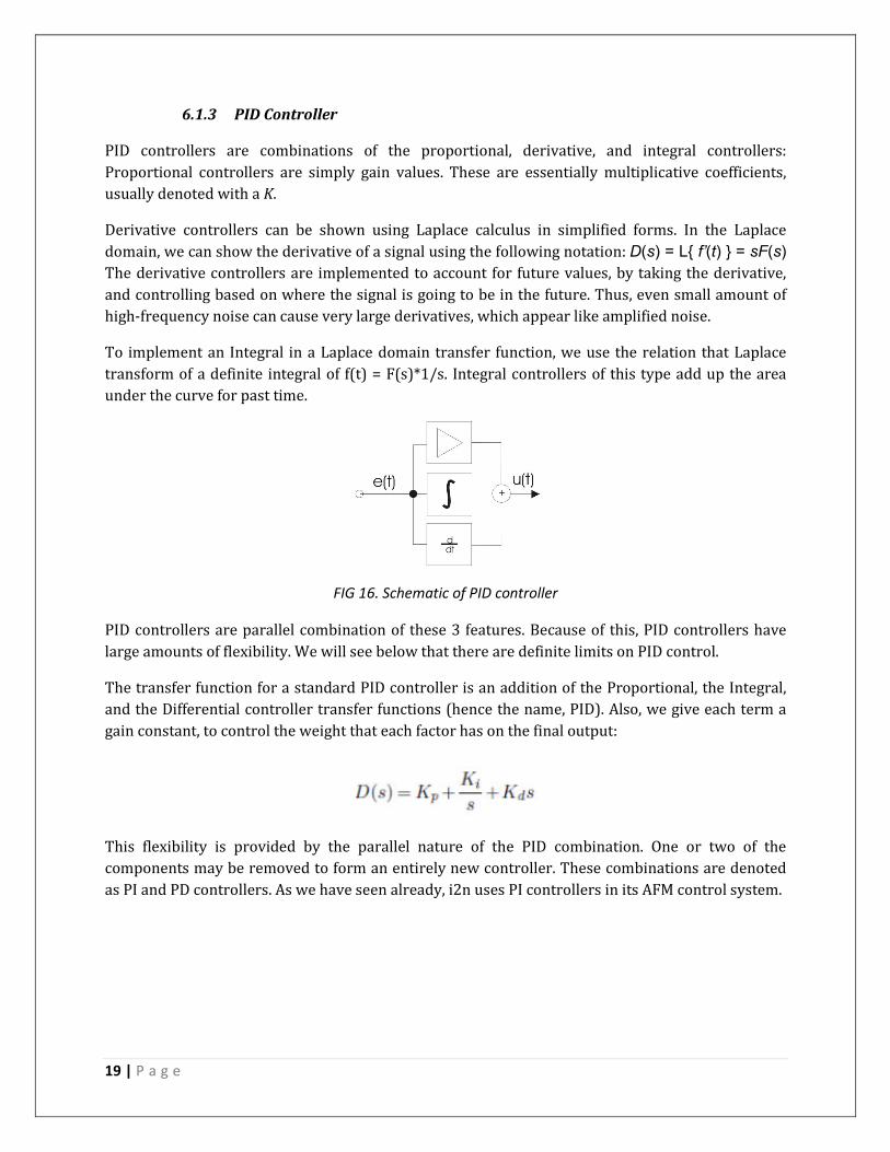
To implement an Integral in a Laplace domain transfer function, we use the relation that Laplace
transform of a definite integral of f(t) = F(s)*1/s. Integral controllers of this type add up the area
under the curve for past time.
FIG 16. Schematic of PID controller
PID controllers are parallel combination of these 3 features. Because of this, PID controllers have
large amounts of flexibility. We will see below that there are definite limits on PID control.
The transfer function for a standard PID controller is an addition of the Proportional, the Integral,
and the Differential controller transfer functions (hence the name, PID). Also, we give each term a
gain constant, to control the weight that each factor has on the final output:
This flexibility is provided by the parallel nature of the PID combination. One or two of the
components may be removed to form an entirely new controller. These combinations are denoted
as PI and PD controllers. As we have seen already, i2n uses PI controllers in its AFM control system.
20 | P a g e
7. SOLUTION METHODOLOGY
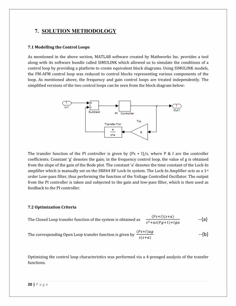
7.1 Modelling the Control Loops
As mentioned in the above section, MATLAB software created by Mathworks Inc. provides a tool
along with its software bundle called SIMULINK which allowed us to simulate the conditions of a
control loop by providing a platform to create equivalent block diagrams. Using SIMULINK models,
the FM-AFM control loop was reduced to control blocks representing various components of the
loop. As mentioned above, the frequency and gain control loops are treated independently. The
simplified versions of the two control loops can be seen from the block diagram below:
The transfer function of the PI controller is given by (Ps + I)/s, where P & I are the controller
coefficients. Constant ‘g’ denotes the gain; in the frequency control loop, the value of g is obtained
from the slope of the gain of the Bode plot. The constant ‘a’ denotes the time constant of the Lock-In
amplifier which is manually set on the SR844 RF Lock-In system. The Lock-In Amplifier acts as a 1st
order Low-pass filter, thus performing the function of the Voltage Controlled Oscillator. The output
from the PI controller is taken and subjected to the gain and low-pass filter, which is then used as
feedback to the PI controller.
7.2 Optimization Criteria
The Closed Loop transfer function of the system is obtained as ��������
������ �� � --{a}
The corresponding Open Loop transfer function is given by ����� ����� --{b}
Optimizing the control loop characteristics was performed via a 4-pronged analysis of the transfer
functions.
21 | P a g e
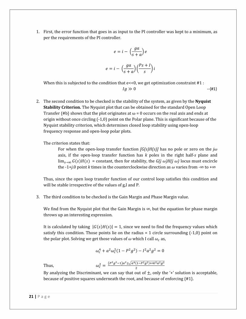
1. First, the error function that goes in as input to the PI controller was kept to a minimum, as
per the requirements of the PI controller.
� � � −� ��� + �� �
� � � −� ��� + �� ��� + �� � �
When this is subjected to the condition that e<<0, we get optimization constraint #1 :
�� ≫ 0 --{#1}
2. The second condition to be checked is the stability of the system, as given by the Nyquist
Stability Criterion. The Nyquist plot that can be obtained for the standard Open Loop
Transfer {#b} shows that the plot originates at ω = 0 occurs on the real axis and ends at
origin without once circling (-1,0) point on the Polar plane. This is significant because of the
Nyquist stability criterion, which determines closed loop stability using open-loop
frequency response and open-loop polar plots.
The criterion states that:
For when the open-loop transfer function [G(s)H(s)] has no pole or zero on the jω
axis, if the open-loop transfer function has k poles in the right half-s plane and lim�→∞ "���#��� = constant, then for stability, the G(j ω)H(j ω) locus must encircle
the -1+j.0 point k times in the counterclockwise direction as ω varies from -∞ to +∞
Thus, since the open loop transfer function of our control loop satisfies this condition and
will be stable irrespective of the values of g,I and P.
3. The third condition to be checked is the Gain Margin and Phase Margin value.
We find from the Nyquist plot that the Gain Margin is ∞, but the equation for phase margin
throws up an interesting expression.
It is calculated by taking |"���#���| � 1, since we need to find the frequency values which
satisfy this condition. Those points lie on the radius = 1 circle surrounding (-1,0) point on
the polar plot. Solving we get those values of ω which I call &' as,
&'( + �)&')�1 − �)�)� − �)�)�) � 0
Thus, &') � *�� �+�,��±.�/��+�� ��(��� �)
By analyzing the Discriminant, we can say that out of ±, only the ‘+’ solution is acceptable,
because of positive squares underneath the root, and because of enforcing {#1}.
22 | P a g e
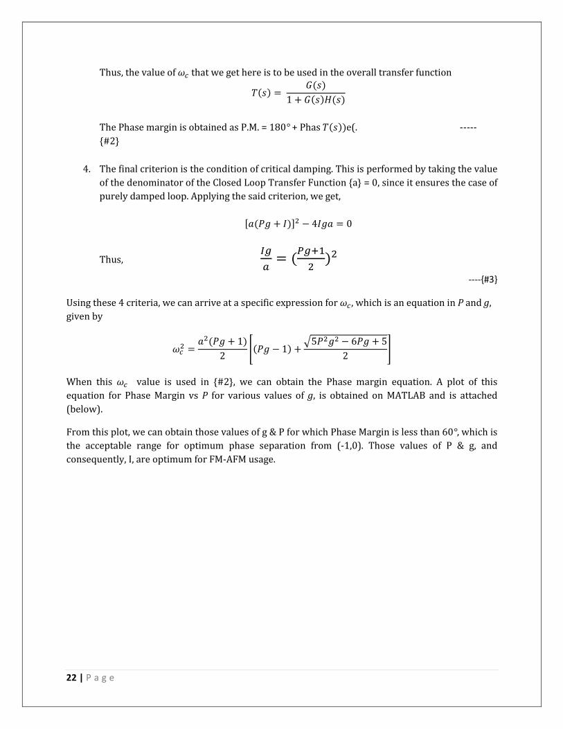
Thus, the value of &' that we get here is to be used in the overall transfer function
0��� � "���1 + "���#���
The Phase margin is obtained as P.M. = 180° + Phas0����e(. -----
{#2}
4. The final criterion is the condition of critical damping. This is performed by taking the value
of the denominator of the Closed Loop Transfer Function {a} = 0, since it ensures the case of
purely damped loop. Applying the said criterion, we get,
1���� + ��2) − 4��� � 0
Thus, � � �� �) �)
----{#3}
Using these 4 criteria, we can arrive at a specific expression for &' , which is an equation in P and g,
given by
&') � �)��� + 1�2 5��� − 1� + .5�)�) − 6�� + 52 8 When this &' value is used in {#2}, we can obtain the Phase margin equation. A plot of this
equation for Phase Margin vs P for various values of g, is obtained on MATLAB and is attached
(below).
From this plot, we can obtain those values of g & P for which Phase Margin is less than 60°, which is
the acceptable range for optimum phase separation from (-1,0). Those values of P & g, and
consequently, I, are optimum for FM-AFM usage.
23 | P a g e
8. CONCLUSION
The developed algorithm predicts to a satisfying degree the coefficients required to optimally tune
the PID controller. The algorithm has been translated to a code which is currently under testing to
reduce errors and include further parameters into the methodology.
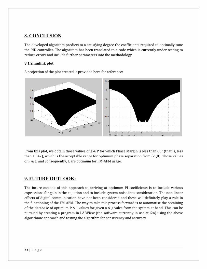
8.1 Simulink plot
A projection of the plot created is provided here for reference:
From this plot, we obtain those values of g & P for which Phase Margin is less than 60° {that is, less
than 1.047), which is the acceptable range for optimum phase separation from (-1,0). Those values
of P & g, and consequently, I, are optimum for FM-AFM usage.
9. FUTURE OUTLOOK:
The future outlook of this approach to arriving at optimum PI coefficients is to include various
expressions for gain in the equation and to include system noise into consideration. The non-linear
effects of digital communication have not been considered and these will definitely play a role in
the functioning of the FM-AFM. The way to take this process forward is to automatise the obtaining
of the database of optimum P & I values for given a & g vales from the system at hand. This can be
pursued by creating a program in LABView (the software currently in use at i2n) using the above
algorithmic approach and testing the algorithm for consistency and accuracy.
24 | P a g e
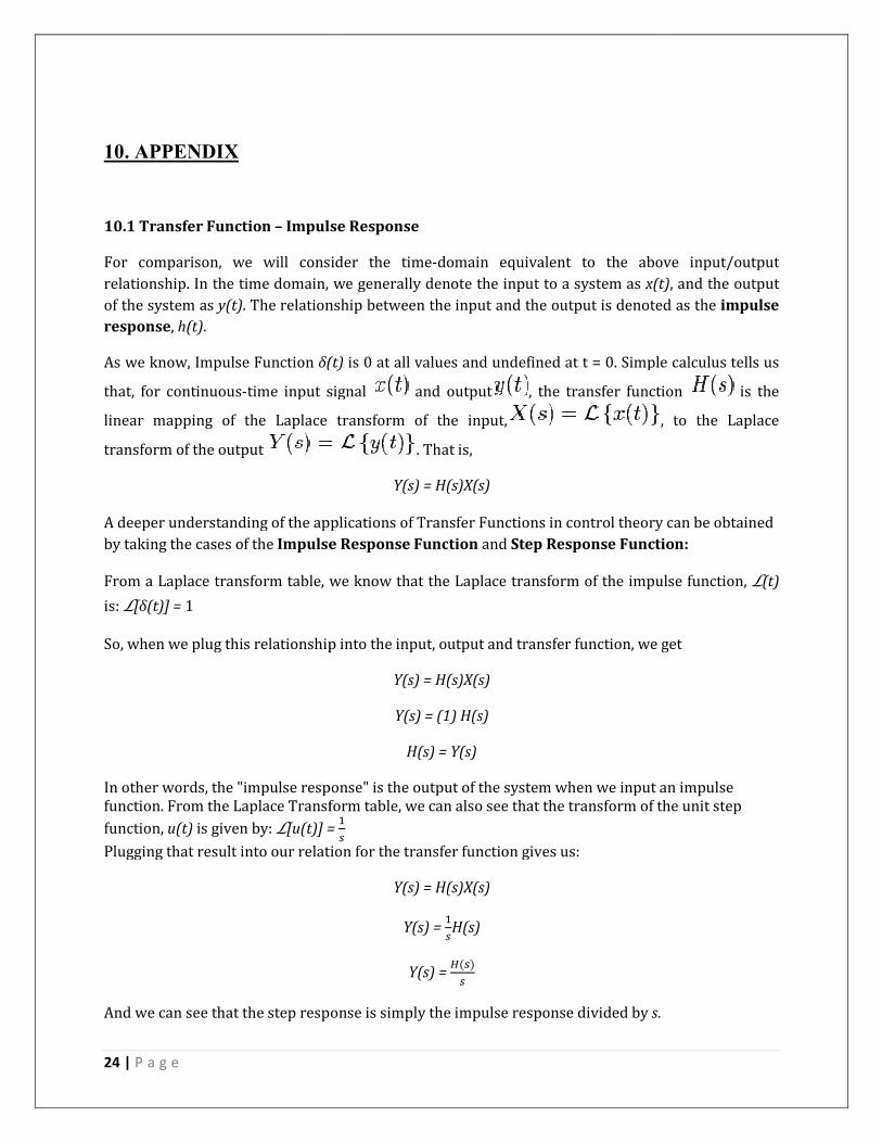
10. APPENDIX
10.1 Transfer Function – Impulse
For comparison, we will consider the time
relationship. In the time domain, we generally denote the input to a system as
of the system as y(t). The relationship between the input and
response, h(t).
As we know, Impulse Function δ(
that, for continuous-time input signal
linear mapping of the Laplace transform of the input,
transform of the output
A deeper understanding of the applications of Transfer Functions in control theory can be obtained
by taking the cases of the Impulse Response Func
From a Laplace transform table, we know that the Laplace transform of the impulse function,
is: L[δ(t)] = 1
So, when we plug this relationship into the input, output and transfer function, we get
In other words, the "impulse response" is the output of the system when we input an
function. From the Laplace Transform table, we can also see that the transform of the unit step
function, u(t) is given by: L[u(t)] =
Plugging that result into our relation for the transfer function gives us:
And we can see that the step response is simply the impulse response divided by
Impulse Response
For comparison, we will consider the time-domain equivalent to the above input/output
relationship. In the time domain, we generally denote the input to a system as x(t)
. The relationship between the input and the output is denoted
δ(t) is 0 at all values and undefined at t = 0. Simple calculus tells us
time input signal and output , the transfer function
of the Laplace transform of the input,
. That is,
Y(s) = H(s)X(s)
A deeper understanding of the applications of Transfer Functions in control theory can be obtained
Impulse Response Function and Step Response Function
From a Laplace transform table, we know that the Laplace transform of the impulse function,
So, when we plug this relationship into the input, output and transfer function, we get
Y(s) = H(s)X(s)
Y(s) = (1) H(s)
H(s) = Y(s)
the "impulse response" is the output of the system when we input an
From the Laplace Transform table, we can also see that the transform of the unit step
)] = ��
Plugging that result into our relation for the transfer function gives us:
Y(s) = H(s)X(s)
Y(s) = ��H(s)
Y(s) = 9����
And we can see that the step response is simply the impulse response divided by s.
domain equivalent to the above input/output
x(t), and the output
the output is denoted as the impulse
is 0 at all values and undefined at t = 0. Simple calculus tells us
, the transfer function is the
, to the Laplace
A deeper understanding of the applications of Transfer Functions in control theory can be obtained
Step Response Function:
From a Laplace transform table, we know that the Laplace transform of the impulse function, L(t)
So, when we plug this relationship into the input, output and transfer function, we get
the "impulse response" is the output of the system when we input an impulse
From the Laplace Transform table, we can also see that the transform of the unit step
.
25 | P a g e
Mathematical modeling of input and output signals and transfer functions of the systems and
components of the control circuit required a simpler method of representation than conventional
linear equations. Thus the Block Diagram system was developed as a tool for easy representation of
classical control loops.
10.2 BODE PLOT, NYQUIST PLOT : MATLAB Simulink TOOL
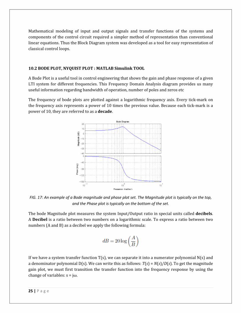
A Bode Plot is a useful tool in control engineering that shows the gain and phase response of a given
LTI system for different frequencies. This Frequency Domain Analysis diagram provides us many
useful information regarding bandwidth of operation, number of poles and zeros etc
The frequency of bode plots are plotted against a logarithmic frequency axis. Every tick-mark on
the frequency axis represents a power of 10 times the previous value. Because each tick-mark is a
power of 10, they are referred to as a decade.
FIG. 17: An example of a Bode magnitude and phase plot set. The Magnitude plot is typically on the top,
and the Phase plot is typically on the bottom of the set.
The bode Magnitude plot measures the system Input/Output ratio in special units called decibels.
A Decibel is a ratio between two numbers on a logarithmic scale. To express a ratio between two
numbers (A and B) as a decibel we apply the following formula:
If we have a system transfer function T(s), we can separate it into a numerator polynomial N(s) and
a denominator polynomial D(s). We can write this as follows: T(s) = N(s)/D(s). To get the magnitude
gain plot, we must first transition the transfer function into the frequency response by using the
change of variables: s = jω.
26 | P a g e
From here, we can say that our frequency response is a composite of two parts, a real part
imaginary part X: T(jω) = R(ω)+jX
The Bode magnitude and phase plots can be quickly and easily appro
straight lines. Once the straight-line graph is determined, the actual Bode plot
that follows the straight lines, and travels through the
Bode plots on MATLAB - This operation can be performed usi
MATLAB also offers a number of tools for examining the frequency response characteristics
system, both using Bode plots, and using Nyquist charts. To construct a Bode plot
function, we use the following command:
[mag, phase, omega] = bode(NUM, DEN, omega);
Or:
[mag, phase, omega] = bode(A, B, C, D, u, omega);
Where "omega" is the frequency vector where the magnitude and phase response points are
analyzed. If we want to convert the magnitude data into
conversion: magdb = 20 * log10(mag);
When talking about Bode plots in decibels, it makes the most sense (and is the most
occurrence) to also use a logarithmic frequency scale. To create such a logarithmic
omega, we use the logspace command, as such:
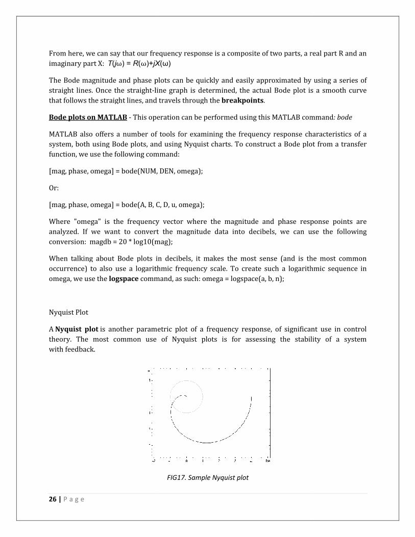
Nyquist Plot
A Nyquist plot is another parametric plot of a frequency response
theory. The most common use of Nyquist plots is for assessing the sta
with feedback.
From here, we can say that our frequency response is a composite of two parts, a real part
jX(ω)
The Bode magnitude and phase plots can be quickly and easily approximated by using a
line graph is determined, the actual Bode plot is a smooth curve
that follows the straight lines, and travels through the breakpoints.
This operation can be performed using this MATLAB command
MATLAB also offers a number of tools for examining the frequency response characteristics
system, both using Bode plots, and using Nyquist charts. To construct a Bode plot
command:
[mag, phase, omega] = bode(NUM, DEN, omega);
[mag, phase, omega] = bode(A, B, C, D, u, omega);
Where "omega" is the frequency vector where the magnitude and phase response points are
analyzed. If we want to convert the magnitude data into decibels, we can use the following
magdb = 20 * log10(mag);
When talking about Bode plots in decibels, it makes the most sense (and is the most
occurrence) to also use a logarithmic frequency scale. To create such a logarithmic
command, as such: omega = logspace(a, b, n);
parametric plot of a frequency response, of significant use in control
The most common use of Nyquist plots is for assessing the stability of a system
FIG17. Sample Nyquist plot
From here, we can say that our frequency response is a composite of two parts, a real part R and an
ximated by using a series of
is a smooth curve
is MATLAB command: bode
MATLAB also offers a number of tools for examining the frequency response characteristics of a
system, both using Bode plots, and using Nyquist charts. To construct a Bode plot from a transfer
Where "omega" is the frequency vector where the magnitude and phase response points are
decibels, we can use the following
When talking about Bode plots in decibels, it makes the most sense (and is the most common
occurrence) to also use a logarithmic frequency scale. To create such a logarithmic sequence in
, of significant use in control
bility of a system
27 | P a g e
In Cartesian coordinates, the real part of the transfer function is plotted on the X axis. The
imaginary part is plotted on the Y axis. The frequency is swept as a parameter, resulting in a plot
per frequency.
Thus, this careful inspection of the Nyquist plot reveals a surprising relationship to the Bode plots
of the system. If we use the Bode phase plot as the angle ϴ, and the Bode magnitude plot as the
distance r, then it becomes apparent that the Nyquist plot of a system is simply the polar
representation of the Bode plots. To obtain the Nyquist plot from the Bode plots, we take the phase
angle and the magnitude value at each frequency ω. We convert the magnitude value from decibels
back into gain ratios. Then, we plot the ordered pairs (r, ϴ) on a polar graph.
The major application of Nyquist plots : the assessment of the stability of a closed-loop negative
feedback system is done by applying Nyquist stability criterion to the Nyquist plot of the open-loop
system. This method is easily applicable even for systems with delays and other non-rational
transfer functions, which may appear difficult to analyze by means of other methods. Stability is
determined by looking at the number of encirclements of the point at (-1,0). Range of gains over
which the system will be stable can be determined by looking at crossing of the real axis.
When drawn by hand, a cartoon version of the Nyquist plot is sometimes used, which shows the
shape of the curve, but where coordinates are distorted to show more detail in regions of interest.
Nyquist plots on MATLAB - This operation can be performed using the MATLAB command nyquist
In addition to the bode plots, we can create nyquist charts by using the nyquist command. The
nyquist command operates in a similar manner to the bode command that we have used so far):
[real, imag, omega] = nyquist(NUM, DEN, omega);
Or:
[real, imag, omega] = nyquist(A, B, C, D, u, omega);
MATLAB TOOL: SIMULINK
Simulink is a data flow graphical programming language tool for modeling, simulating and
analyzing multi-domain dynamic systems. Its primary interface is a graphical block diagramming
tool and a customizable set of block libraries. It offers tight integration with the rest of
the MATLAB environment and can either drive MATLAB or be scripted from it.
Learning this graphical interface language was the final crucial step before embarking upon the
solution to our problem at hand. Simulink allowed one to model the PI controller components and
easily generate Bode, Nyquist and Impulse response simulation plots for quick access.
28 | P a g e
11. REFERENCES
1. Katsuhiko Ogata, Modern Control Engineering, Edition 5, 2011
2. Zhang, Miao, Zheng, Dong, Xi, Feedback Control Implementation for AFM Contact-Mode
Scanner, 2008, 3rd IEEE Int. Conf. on Nano/Micro Engineered and Molecular Systems, IEEE
3. Abramovitch, Andersson, Pao, Schitter, A Tutorial on the Mechanisms, Dynamics, and Control
of Atomic Force Microscopes, 2007, American Control Conference Journal, IEEE
4. Freidt and Carry, Introduction to the quartz tuning fork, 2007, American Journal of Physics,
AAPT
5. Kilpatrick, Gannepalli, Cleveland, Jarvis, Frequency modulation atomic force microscopy in
ambient environments utilizing robust feedback tuning, 2009, RSI, Am. Inst. Of Physics
6. Hrouzek, Feedback Control in an Atomic Force Microscope Used as a Nano-Manipulator,
2005, Acta Polytechnica
7. Bueno, Balthazar, Piquiera, Phase-Locked Loop Application to Frequency Modulation - Atomic
Force Microscope, 2010, Bra. Conf. on Dynamics, Control and Applications
8. Edwards, Taylor, Duncan, Fast, high-resolution atomic force microscopy using a quartz tuning
fork as actuator and sensor, 1997, OJPS, American Institute Of Physics
9. Singh, Kumar, Electronics and Software for Scanning Tunneling Microscope, Inter-
Universoty Accelerator Centre
10. Control Systems, Wikibooks Creative Commons Attribution-ShareAlike 3.0 Unported license