COINTEGRATION ANALYSIS OF GERMAN AND BRITISH TOURISM DEMAND FOR GREECE Dr

COINTEGRATION ANALYSIS OF GERMAN AND BRITISH

TOURISM DEMAND FOR GREECE

Dr. Nikolaos Dritsakis

Associate Professor

University of Macedonia

Economics and Social Sciences

Department of Applied Informatics

156 Egnatia Street

P.O box 1591

540 06 Thessaloniki, Greece

FAX: (031) 891290

e-mail: [email protected]

2

COINTEGRATION ANALYSIS OF GERMAN AND BRITISH

TOURISM DEMAND FOR GREECE

Abstract

Germany and Great Britain are traditionally two of the most important sources

of tourism for Greece. The purpose of this paper is to investigate changes in the

long-run demand for tourism to Greece by these two countries. In order to explain

the demand for tourism, we are using a number of leading macroeconomic

variables, including income in origin countries (Germany and Great Britain),

tourism prices in Greece, and transportation cost and exchanges rates between the

three countries. Annual data from the three countries, covering the period from

1960 to 2000, are employed. Augmented Dickey-Fuller test for unit root is

examined in the univariate framework and Johansen’s maximum likelihood

procedure is used to test the cointegration method and to estimate the number of

cointegrating vectors of VAR model. Error correction models are estimated to

explain German and British demand for tourism to Greece.

Keywords: tourism demand, cointegration analysis, error correction model,

1. Introduction

Tourism is an important source of income for many countries - especially for

those with less developed modern service/industrial based economies. The

economic benefits accruing to both the producers of tourist products and the

3

tourist originating economy in local, regional and national level have been the

subject of extensive studies by both tourism experts and multidisciplinary

scholars.

Tourist destinations have an a priori concentration of tourism related “raw

materials”. In this case raw materials refer mainly to a combination of natural and

man-made elements that are related closely with tourism demand and, unlike other

aspects of economic activity, are unique to the tourism destination and therefore

cannot be transferred to or recreated at another location. It is well known that

natural and climatic factors play the primary role in choosing a holiday

destination. However, apart from favourable natural and climatic factors, man-

made factors – such as culture, heritage or results of human activity- also play an

important role in the decision for a tourist destination that can be supplementary to

or independent of the “raw materials” in the destination (Dritsakis 1995, Seddighi

et al 2001, Seddighi and Theocharous 2002).

The existence of favourable natural and climatic conditions in a country or

(and) rich cultural evidence does not automatically guarantee its choice as a

popular tourist destination. It must first ensure that a minimum level of tourism

provision is in place, such as adequate infrastructure and, most important, a

reasonably priced tourist product.

Due to its unique combination of both the aforementioned factors, Greece is a

popular tourist destination with most of the European countries. Germany and

Great Britain are the major originators of tourists for Greece.

Over the period 1960-2000, total tourist arrivals to Greece grew at an average

rate of 2.4% per annum. Tourist arrivals from Europe form the main part of

foreign visitors in Greece. Germany is the most important source of tourists for

4

Greece and over the examined period had an average annual growth rate of tourist

arrivals to Greece 3.2% per annum. The average annual growth rate of tourist

arrivals from Great Britain (the second biggest source of tourists), was 3.1% per

annum for the same period.

In this paper a cointegration analysis of multivariate time series is presented,

where some time series are modelled simultaneously and we have a priori

knowledge for the expected signs of the variables examined. Economic variables

such as income, tourism prices, cost of transportation and exchange rates are

examined in order to explain tourist arrivals from Germany and Great Britain to

Greece.

Many time series models like Box-Jenkins ARIMA model that do not have

explicit economic context but arise empirically, are used to explain the level of

tourist arrivals (Johnson and Ashworth 1990, Morley 1992, Syriopoulos 1995,

Lim 1997, Lim and McAller 2000a, 2000b). The changes in tourist arrivals are

exclusively related to their past levels or are time-dependent. Nevertheless, the

econometric models that explain the structure of tourist arrivals by a specific

origin country can also combine present and past values of the other economic

variables with tourist arrivals (Witt and Witt 1995, Song and Witt 2000, Dritsakis

and Athanasiadis 2000).

The rest of the paper is organized as follows: section 2 describes the data used

for the tourism demand analysis for Greece. Section 3 describes the results of the

unit root test. Section 4 briefly outlines the cointegration analysis and Johansen’s

test for cointegration. Section 5 presents the empirical results of tourism demand

to Greece from Germany and Great Britain. Section 6 discusses the error

5

correction models for travel to Greece from Germany and Great Britain. Finally,

section 7 presents some conclusive remarks.

2. Data

In the analysis of tourism demand to Greece from Germany and Great Britain

the following function is used:

AR=F(Y,TP,TR,ER) (1)

where (AR) expresses tourist arrivals from every origin country, (Y) the real

income per capita, (TP) tourism prices, (TR) transportation cost, (ER) exchange

rates between the origin and destination countries’ currencies. The sample period

under consideration is 1960 to 2000. All variables are expressed in logarithms to

capture multiplicative time series effects and are denoted with letter L preceding

each variable name.

Data real income variables include real Gross Domestic Product (GDP) per

capita, real private consumption expenditure per capita, real private expenditure

on consumption services per capita at 1990 prices.

Tourism prices, which include the cost of goods and services purchased by

tourists in the destination country, are measured by relative prices or real exchange

rates (Witt and Martin 1987, Dritsakis and Gialitaki 2001). The relative price

variable is given by the indicative ratio of the consumer price indices (CPI) of the

destination country to the origin countries. The logarithm of relative prices (LTP)

indicates the difference between the logarithm of prices level in Greece and origin

countries for the examined period in this paper.

6

( )( ) )(log)(loglog OriginCPIGRCPIOriginCPI

GRCPILTP −=

=

The average economy class airfare prices of different airport companies from

the origin country to Athens are used as proxies for transportation costs of the two

origin countries of tourists. (These data have been obtained from the Greek

national carrier, Olympic Airways).

The real exchange rate measures the effective prices of goods and services in

destination country, when consumer price index adjusts between the exchange

rates differences in currencies of origin and destination countries. Nominal

exchange rate ER is expressed by the number of units of origin country’s currency

that are needed for the purchase of one drachma. The real exchange rate is given

by the logarithm of prices level in Greece minus the logarithm of prices level in

origin countries minus the logarithm of exchange rate.

EROriginCPIGRCPIEROriginCPI

GRCPILER log)(log)(log1)(

)(log −−=

•=

where ER= the exchange rates in units of origin country’s currency that are

needed for the purchase of one drachma

Data sources include the National Statistical Service of Greece, IMF

International Financial Statistics, the World Bank, the Bank of Greece and

databases of Datastream and EconData.

Although marketing spending and special promotions are expected to play an

important role in attracting tourists from these two countries to Greece, there is no

appropriate information for the expenditure involved in each country.

7

The Greek Tourism Organization is responsible for Greece’s tourism marketing

strategy and spending in all European countries. Unfortunately the breakdown of

the total promotional expenditure per country is not available.

The list of variables used in the analysis of German and British tourism demand

for Greece is as follows:

LAR= Logarithm of tourist arrivals from an origin country to Greece.

LY= Logarithm of real gross domestic product per capita.

LTP= Logarithm of relative prices (tourism prices).

LTR=Logarithm of real airfares prices in the origin country’s currency

(transportation cost).

LER= Logarithm of real exchange rate or exchange rate of adjusted relative

prices.

The examination of variables’ plots suggests that tourist arrivals, real income

per capita, tourism prices, transportation costs, and real exchange rates appear to

be non-stationary and contain a predetermined stochastic trend. This means that

these specific variables contain important information to explain the changes in

tourist arrivals to Greece. In the underlying economic framework, the demand for

international travels is positively related to income in the origin countries, and

negatively related to tourism prices, transportation costs and real exchange rates of

the origin country. The variables may drift apart in the short-run but should move

together in the long-run.

If these variables share a common stochastic trend, their first differences are

stationary and consequently may be jointly cointegrated. Economic theory does

not often provide guidance in determining which variables have stochastic trends,

and when such trends are common among variables. For multivariate time series

8

analysis involving stochastic trends, augmented Dickey-Fuller unit root tests are

calculated for individual time series to provide evidence as to whether the

variables are integrated. This is followed by multivariate cointegration analysis.

3. Unit root test

Testing for cointegration among several variables that are used in the above

model needs primarily a test for the presence of unit root for every individual

variable, namely real tourism arrivals, gross domestic product, tourism prices,

transportation costs, real exchange rates, using the Augmented Dickey-Fuller test

(ADF) (1979) based on the auxiliary regression:

∑=

−− +∆+++=∆k

itttt uyyty

111 γβδα (2)

The ADF auxiliary regression tests for the existence of a unit root in yt, namely

the logarithm of all model’s variables at time t. The variable ∆yt-1 expresses the

lagged first differences, ut adjusts the serial correlation errors and α, δ, β and γ are

the parameters to be estimated. The null and alternative hypotheses for a unit root

in variable yt are:

Ηο : β = 0 Ηε : β < 0

The tests are performed sequentially. First, the ADF test is calculated for the

sample period, with and without a deterministic trend. The time trend is included

in the auxiliary regression equation if the reported ADF t-statistics show that the

9

regression is statistically significant. If time trend is not included in the examined

variables, then the regression equation will reduce the power of the test. A

sufficient number of lagged first differences are included to remove any serial

correlation in the residuals. In order to determine k, an initial lag length of 4 is

selected, and the fourth lag is tested for significance using the standard asymptotic

t-ratio. If the fourth lag is insignificant, the lag length is reduced successively until

a significant lag length is obtained. If no lagged first differences are used, the ADF

test reduces to the Dickey-Fuller (DF) test. The MFIT 4.0 (1997) software

package, which is used to conduct the ADF tests, reports the simulated critical

values.

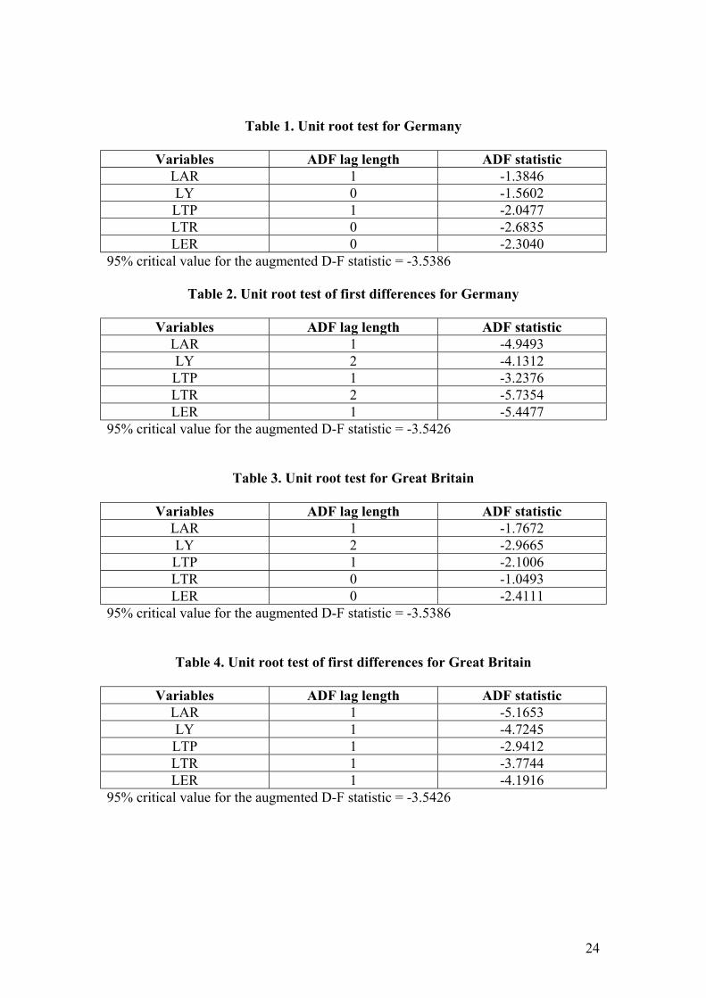
Table 1 presents the results of the ADF tests of real tourist arrivals, real income

per capita, tourism prices, transportation costs and exchange rate for Germany.

The ADF tests statistics are compared with the critical value from the non-

standard Dickey-Fuller distribution with time trend at the 5% level significance.

The calculated ADF statistics for all variables exceed the critical value. This

means that none of all variables is stationary. Thus, the null hypothesis of a unit

root is not rejected.

INSERT TABLE 1 APPROXIMATELY HERE

Table 2 shows that, with the exception of LTP, taking first differences renders

each series stationary, with the ADF statistics in all cases being less than the

critical value at 5% level significance. The result for the variable LTP is sensitive

to the choice of lag length. At the one lag, the null hypothesis of a unit root is still

not rejected. However, at zero lags the null hypothesis of a unit root is rejected.

10

The Akaike Information Criterion (AIC) (1973) and the Schwarz Bayesian

Criterion (SBC) (1978) yield smaller values for one lag. By taking the second

differences, LTP becomes a stationary time series. The ADF test for the individual

series of Germany indicates that all variables are integrated order one I(1), apart

from tourism prices (LTP) that are integrated with order two I(2). Therefore,

tourism prices of Germany are not cointegrated with the other time series.


According to Table 3, the null hypothesis of a unit root test is not rejected for

all variables for Great Britain. By taking first differences Table 4 shows that all

time series become stationary as the ADF statistic for each time series (except

LPT) is lower than the relative critical value at a 5% level significance. The

variable LPT becomes stationary in second differences. From these results we can

infer that all variables are integrated order 1 I(1), but tourism prices (LPT) are

integrated order 2 I(2). Consequently, tourism prices of Great Britain are not

cointegrated with the other time series.



4. Cointegration and Johansen test

If time series variables are nonstationary in their levels they are integrated (of

order one) and their first differences are stationary. These variables may also be

cointegrated if there exists one or more linear combinations among them that is

11

stationary. If these variables are cointegrated, then there is a stable long run or

equilibrium linear relationship among them. For instance, if tourist travel demand

as measured by tourist arrivals to a certain destination, and real income are not

cointegrated, then the tourist arrivals would drift above or below income in the

long-run. Granger (1986, p.226) argued that ‘A test for cointegration can thus be

thought of as a pre-test to avoid ‘‘spurious regression’’ situations’. Furthermore,

Engle and Granger (1987, p.264) prescribed that ‘it may not be so easy to test

whether a set of variables are cointegrated before estimating a multivariate

dynamic model.’

Cointegration and error correction models are closely related. Engle and

Granger (1987, p.254) defined error correction as ‘a proportion of the

disequilibrium from one period is corrected in the next period’. An error

correction model relates the change in one variable to past equilibrium errors.

If the hypothesis of a unit root is not rejected, then a test for cointegration is

performed. The hypothesis being test is the null of noncointegration against the

alternative of cointegration, using Johansen’s maximum likelihood method. A

vector autoregression approach is used to model each variable (which is assumed

to be jointly endogenous) as a function of all the lagged endogenous variables in

the system. Johansen (1988) considers a simple case where Xt is integrated of

order one, such that the first difference of Xt is stationary.

Suppose the process Xt is defined by an unrestricted VAR system of order

(n×1)

tktkttt uXXXX +Π++Π+Π= −−− ..........2211 (3)

where Xt = (n × 1) vector of Ι(1) variables

Πi = (n × n) matrix of unknown parameters to be estimated (i = 1, 2, 3,…..k).

12

ut = independent and identically distributed (n × 1) vector of error terms.

t = 1, 2, 3……T observations

Using ∆ = (Ι – L), where L is the lags operator the system of above can be

reparameterized in the error correction form as:

∑−

=−− +Π+∆Γ=∆

1

1

k

itktitit uXXX (4)

where ∆Χt = is an Ι(0) vector.

Ι = is an (n × n) identity matrix

∑−

=

−Π=Γ1

1

k

iii I i = 1, 2,……………k-1.

and

∑=

−Π=Πk

jj I

1

The above equation (4) is known as a vector error correction (VEC) model.

Johansen’s approach derives maximum likelihood estimators of the

cointegrating vectors for an autoregressive process with independent errors. The (n

× n) matrix Π can be written as the product of α and β, two (n × r) matrices each of

rank r, such that Π = βα′, where α contains the r cointegrating vectors and β

represents the matrix of weighting elements. Hence the above equation can be

written as:

∑−

=−− ++∆Γ=∆

1

1

' )(k

itktitit uXXX βα

The maximum likelihood approach enables testing the hypothesis of r

cointegrating relations among the elements of Xt.

Ηο : Π = βα′

13

where the null hypothesis of no cointegrating relations (r = 0) implies Π = 0. Thus,

test for cointegration test whether the eigenvalues of the estimated Π are

significantly different from 0. This approach also tests for the number of

cointegrating relations, where 0 r≤ < n. If there is no cointegrating relation, then

no linear combination of nΙ(1) variables is stationary.

Johansen’s method maximizes the likelihood function for Χt, conditional on

any given α, using standard least squares formulae for the regression of ∆Χt on the

lagged differences ∆Χt-1, ∆Xt-2……, ∆Xt-k+1 and α΄X t-k. This approach provides

estimates of Γ1, Γ2,…..Γk-1 and β, conditional on α and can also be used to test

which cointegrating vectors are statistically significant.

In the empirical section below, the number of cointegrating relations among the

Ι(1) variables of the used model are presented.

5. Empirical results

Most variables that have been used in the model reported in the last section as

tourist arrivals (LAR), real income per capita (LY), transportation cost (LTR), real

exchange rate (LER) of demand for travel to Greece that come from Germany and

Great Britain are integrated of order 1, I(1). Therefore, they can be cointegrated on

a VAR model up to four lags. As the lag intervals are specified as range pairs, this

means that lags of the first differences are used, the highest lag in their levels is

order 5. Thus, if lag intervals 1 to 4 are chosen the VAR model applies the

regression analysis ∆Υt on ∆Υt-1 ∆Υt-2, ∆Υt-3, ∆Υt-4 and contain four variables. In

implementing the Johansen procedure, a linear deterministic trend and intercept

are included in the cointegrating equation.

14

The order of r is determined by using the likelihood ratio (LR) trace test

statistic suggested by Johansen (1988).

λtrace(q,n) = -T ∑+=

−k

qii

1)ˆ1ln( λ (5)

for r = 0, 1, 2,…….k-1,

Τ = the number of observation used for estimation

=iλ̂ is the ith largest estimated eigenvalue.

Critical values for the trace statistic defined by equation (5) are 58.93 and 55.01

for Ηο: r = 0 and 39.33 and 36.28 for Ηο: r ≤ 1 at the significance level 5% and

10% respectively as reported by Osterwald-Lenum (1992).

The maximum eigenvalue LR test statistic as suggested by Johansen is:

λmax(q, q+1) = -Tln(1- )ˆ1+qλ (6)

The trace statistic either rejects the null hypothesis of no cointegration among

the variables (r=0) or does not reject the null hypothesis that there is one

cointegrating relation between the variables (r≤1). Tables 5 and 6 present the

results for all systems of equations, each with one cointegrating relation, in which

the coefficients of the variables are significant at the 5% level and have the correct

signs. As AIC tends to select the larger lag length and SBC the more parsimonious

VAR an LR test was used to select the appropriate lag length. The null hypothesis

that a system is generated by a Gaussian VAR with p0 lags, against the alternative

specification of p1>p0 is tested by the LR test statistic, which is computed as:

LR = -2(l0 – li)

where li (i = 0,1) is the log-likelihood reported in the VAR model with pi (i = 0, 1)

lags. Under Η0, the LR test statistic is asymptotically distributed as Χ2, with

15

n2(pi – p0) degrees of freedom. The null hypothesis imposes n2(pi – p0) restrictions,

where n = number of variables.

Based on the smallest AIC and SBC values, the trace test results for one

cointegrating equation involving four variables are presented in Table 5 and 6.

When normalized for a unit coefficient on tourist arrivals (LAR) the most

appropriate cointegrating regression of the long-run demand for international

travel by tourists that come from Germany and Great Britain respectively, is given

by VAR(3) models as follows (with absolute asymptotic t-ratios in parentheses):

LAR = -36.3465 + 2.1592 LY – 0.6155 LTR – 0.9881 LER (7)

(-6.3292) (3.8956) (-6.4175) (-2.6040)

LAR = 0.11357 + 6.0268 LY – 1.4031 LTR – 1.1990 LER (8)

(2.1694) (7.3703) (-2.6412) (-4.3809)



The coefficient estimates in the equilibrium relation which are the estimated

long-run elasticities with respect to tourist arrivals, show that real income per

capita is elastic, while real costs (as measured by the logarithm of airfares) and

real exchange rate are both inelastic for tourist arrivals from Germany, while all

coefficients by their estimations in equilibrium relationship are elastic to tourist

arrivals from Great Britain.

16

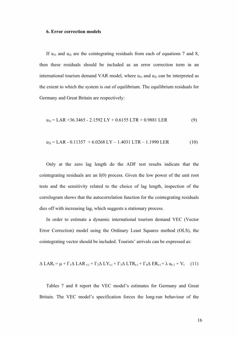
6. Error correction models

If u1t and u2t are the cointegrating residuals from each of equations 7 and 8,

then these residuals should be included as an error correction term in an

international tourism demand VAR model, where u1t and u2t can be interpreted as

the extent to which the system is out of equilibrium. The equilibrium residuals for

Germany and Great Britain are respectively:

u1t = LAR +36.3465 - 2.1592 LY + 0.6155 LTR + 0.9881 LER (9)

u2t = LAR - 0.11357 + 6.0268 LY – 1.4031 LTR – 1.1990 LER (10)

Only at the zero lag length do the ADF test results indicate that the

cointegrating residuals are an I(0) process. Given the low power of the unit root

tests and the sensitivity related to the choice of lag length, inspection of the

correlogram shows that the autocorrelation function for the cointegrating residuals

dies off with increasing lag, which suggests a stationary process.

In order to estimate a dynamic international tourism demand VEC (Vector

Error Correction) model using the Ordinary Least Squares method (OLS), the

cointegrating vector should be included. Tourists’ arrivals can be expressed as:

∆ LARt = µ + Γ1∆ LAR t-i + Γ2∆ LΥt-i + Γ3∆ LTRt-i + Γ4∆ ERt-i + λ ut-1 + Vt (11)

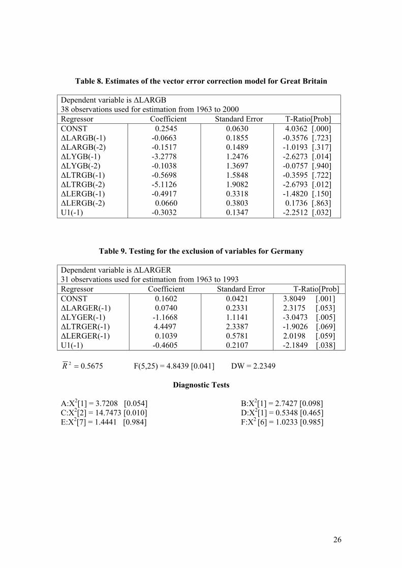
Tables 7 and 8 report the VEC model’s estimates for Germany and Great

Britain. The VEC model’s specification forces the long-run behaviour of the

17

endogenous variables to converge to their cointegrating relationships, while

accommodating short-run dynamics. The dynamic specification of the model

suggests deleting the insignificant variables until a regression with all its

coefficients statistically significant will be obtained.



A subset of the variables is tested for statistical significance to examine if they

can be omitted from the model. The associated tests statistics reported include the

F-statistic and the log-likelihood ratio statistic. Each of the insignificant variables

is deleted sequentially from the general dynamic model, while the error correction

model is retained, which is statistically significant at 5% level. The tests statistics

do not reject the null hypothesis that the selected coefficients are jointly zero at the

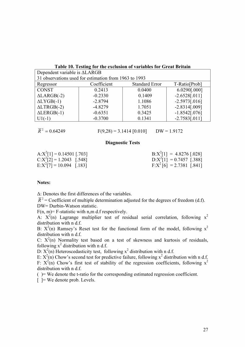
5% significance level. By deleting the statistically insignificant regressors, Tables

9 and 10 are obtained with all variables statistically significant and the coefficients

in error correction terms are negative and statistically significant as well. The

estimated coefficients of error correction terms measure the speed of adjustment to

restore equilibrium in the dynamic model. The negative sign of the estimated

coefficients of income is explained by the fact that German and English tourists

(with higher income level), may prefer other tourist destinations than Greece. For

example they may prefer more developed tourist countries, some tourists prefer

over Atlantic destinations in exotic countries and other tourists like travelling to

more safe destinations. Political stability and suppression of terrorism are basic

preconditions for the tourist's safety.

18

We also apply a number of diagnostic tests on the residuals of the model. We

apply the Lagrange test (A) for the residuals’ autocorrelation, the Heterosce-

dasticity test (D) and the Bera-Jarque (C) normality test. We also test the

functional form of the model according to the Ramsey’s Reset test. Chow’s first

and second tests check the model’s predictive ability. Tables 9 and 10 indicate that

all diagnostic tests are statistically significant for both countries in selected VEC

models.



7. Conclusions

The relationships among the demand for travelling, income of origin country,

tourism prices, transportation costs and exchange rates have received considerable

attention in empirical tourism research (Dritsakis and Papanastasiou 1998, Lim

1999). Even though it is well known empirically that many macroeconomic time

series are nonstationary, most published tourism research has estimated static

models in logarithmic levels using ordinary least squares. This practice gives rise

to invalid inferences, so there is little informational content in examining the

alleged significance of the estimated coefficients.

Cointegration techniques permit the estimation and testing of the long-run

equilibrium relationships, as suggested by economic theory. Vector error

correction (VEC) models provide a way of combining both the dynamics of the

short run (changes) and long-run (levels) adjustment processes simultaneously.

19

Using separate tourist arrivals data from Germany and Great Britain to Greece

as measures of tourism demand from these countries, the long-run economic

relationships among international tourism demand real income, transportation cost

and exchange rates have been estimated. Prior to testing for cointegration among

a set of variables, the ADF test of nonstationarity is performed to determine the

order of integration of the individual time series. Johansen’s maximum likelihood

procedure is used for estimation and testing of the cointegrating relations based on

vector autoregressive models.

The methods used, and the results presented in this paper, provide some useful

insights into the effects of income, tourism prices, transportation cost and

exchange rate on international tourism demand to Greece from the two most

important origin countries of Europe.

The existence of a long-run equilibrium relationship among international

tourism demand, income, transportation cost and real exchange rate appear to be

supported by the data used for the examined period. According to the theory of

cointegration, the estimated cointegrating residual should appear as the error

correction term in a dynamic VEC model. An important finding from the dynamic

models presented is that the error correction terms are negative and statistically

significant. All regressors in the VEC models are statistically significant, there is

no evidence of any problems associated with serial correlation, functional form,

normality, heteroscedasticity. Given a statistically significant error correction

model in a dynamic VEC model, it can be interpreted as evidence supporting

cointegration, which suggests the existence of an equilibrium long-run relationship

among important economic variables determining international tourism demand.

20

References

Akaike, H. (1973). Information Theory and an Extension of the Maximum

Likelihood Principle, In: Petrov, B. and Csake, F. (eds) 2nd International

Symposium on Information Theory. Budapest: Akademiai Kiado.

Dickey, D.A and Fuller, W.A (1979). Distributions of the Estimators for

Autoregressive Time Series with a Unit Root. Journal of the American Statistical

Association, 74, 427 – 431.

Dritsakis. N. (1995). An economic analysis of foreign tourism to Greece.

Sakkoulas, Thessaloniki.

Dritsakis, N and Papanastasiou, J (1998). An econometric investigation of

Greek tourism, Journal studies in economics and econometrics, 22, 15-122.

Dritsakis, N and S. Athanasiadis (2000). An econometric model of tourist

demand: The case of Greece. Journal of hospitality & leisure marketing, Vol. 2.

39 - 49.

Dritsakis, N. and A. Gialitaki (2001). The tourist demand in the area of Epirus

through cointegration analysis. International Center for Research and Studies in

Tourism, Vol. 8.

21

Engle, R. F, and, C. W. J Granger (1987). Cointegration and error correction:

Representation, estimation and testing. Econometrica, 55, 251 – 276.

Granger, C. W. J (1986). Developments in the study of cointegrated economic

variables, Oxford Bulletin of Economic and Statistics, 48, 213 – 228.

Johansen, S (1988). Statistical analysis of cointegration vectors, Journal of

Economic Dynamics and Control, 12, 231 – 254.

Johnson P. and Ashworth , J. (1990). Modelling tourism demand: A summary

review". Leisure Studies 9, 145 ¯ 160.

Lim , C. (1997). Review of international tourism demand models. Annals of

Tourism Research, 24 (4), 835 ¯ 849.

Lim , C. (1999). A metal-analytic review of international tourism demand,

Journal of Travel Research, 37, 273-84.

Lim, C. and McAller (2000a). A seasonal analysis of Asian tourist arrivals to

Austalia. Applied Economics, 32, 499 – 509.

Lim, C. and McAller (2000b). Monthly seasonal variations: Asian tourism to

Australia. Annals of Tourism Research, 28(1), 68 – 82.

22

MFIT 4.0 (1997). Quantitative Micro Software. Interactive Econometric

Analysis, Oxford University Press.

Morley, C. (1992). A microeconomic theory of international tourism demand.

Annals of Tourism Research, 19, 250 ¯ 267.

Osterwald-Lenum, M. (1992) A note with quantiles of the asymptotic

distribution of the maximum likelihood cointegration rank test statistics, Oxford

Bulletin of Economics and Statistics, 54, 461- 472.

Schwarz, R. (1978). Estimating the Dimension of a Model. Annals of Statistics.

6, 461 – 464.

Seddighi H.R.,. Nuttall M.W and. Theocharous, A.L, (2001). Does cultural

background of tourists influence the destination choice? An empirical study with

special reference to political instability, Tourism Management, 22 (2), 181 ¯ 191.

Seddighi H. R. and Theocharous A. L. (2002), A model of tourism destination

choice: a theoretical and empirical analysis, Tourism Management, 23, 475 - 487.

Song H. and Witt, F.S. (2000). Tourism demand modelling and forecasting.

Modern econometric approaches (1st ed.), Pergamon, New York.

Syriopoulos , T.C. (1995). A dynamic model of demand for mediterranean

tourism, International Review of Applied Economics 9 (3), 318 ¯ 336.

23

Witt , S. F and C. A. Martin (1987). Tourism demand forecasting models:

choice of an appropriate variable to represent tourists cost of living. Tourism

Management, 8, 233 - 246.

Witt S.F. and Witt C.A. (1995). Forecasting tourism demand: A review of

empirical research. International Journal of Forecasting 11 (3), 447 ¯ 475.

24

Table 1. Unit root test for Germany

Variables ADF lag length ADF statistic LAR 1 -1.3846 LY 0 -1.5602 LTP 1 -2.0477 LTR 0 -2.6835 LER 0 -2.3040

95% critical value for the augmented D-F statistic = -3.5386

Table 2. Unit root test of first differences for Germany



Table 3. Unit root test for Great Britain



Table 4. Unit root test of first differences for Great Britain



25

Table 5 Johansen and Juselious trace test for one Cointegration equation for Germany

Variables LAR, LY, LTR, LER,

Maximum lag in VAR = 3 Trace Statistic Critical Values Null Alternative Trace 95% 90% AIC SBC r = 0 r = 1 63.7525 58.9300 55.0100 249.90 236.79 r ≤ 1 r ≥ 2 26.4617 39.3300 36.2800

Table 6 Johansen and Juselious trace test for one Cointegration equation for Great Britain

Variables LAR, LY, LTR, LER,

Maximum lag in VAR = 3 Trace Statistic Critical Values Null Alternative Trace 95% 90% AIC SBC r = 0 r = 1 59.8234 58.9300 55.0100 253.58 240.69 r ≤ 1 r ≥ 2 23.1725 39.3300 36.2800

Table 7. Estimates of the vector error correction model for Germany

Dependent variable is ∆LARGER 38 observations used for estimation from 1963 to 2000 Regressor Coefficient Standard Error T-Ratio[Prob] CONST ∆LARGER(-1) ∆LARGER(-2) ∆LYGER(-1) ∆LYGER(-2) ∆LTRGER(-1) ∆LTRGER(-2) ∆LERGER(-1) ∆LERGER(-2) U1(-1)

0.1806 0.1412 0.0562 -1.4247 -0.5819 -5.6529 -1.2056 0.2839 -0.0870 -0.5124

0.0518 0.2149 0.2083 1.0780 1.0575 2.2556 2.1748 0.4462 0.4222 0.1902

3.4860 [.002] 0.6572 [.516] 0.2700 [.789] -1.3216 [.197] -0.5503 [.586] -2.5062 [.018] -0.5543 [.584] 0.6363 [.530] -0.2061 [.838] -2.6934 [.012]

26

Table 8. Estimates of the vector error correction model for Great Britain

Dependent variable is ∆LARGB 38 observations used for estimation from 1963 to 2000 Regressor Coefficient Standard Error T-Ratio[Prob] CONST ∆LARGB(-1) ∆LARGB(-2) ∆LYGB(-1) ∆LYGB(-2) ∆LTRGB(-1) ∆LTRGB(-2) ∆LERGB(-1) ∆LERGB(-2) U1(-1)

0.2545 -0.0663 -0.1517 -3.2778 -0.1038 -0.5698 -5.1126 -0.4917 0.0660 -0.3032

0.0630 0.1855 0.1489 1.2476 1.3697 1.5848 1.9082 0.3318 0.3803 0.1347

4.0362 [.000] -0.3576 [.723] -1.0193 [.317] -2.6273 [.014] -0.0757 [.940] -0.3595 [.722] -2.6793 [.012] -1.4820 [.150] 0.1736 [.863] -2.2512 [.032]

Table 9. Testing for the exclusion of variables for Germany

Dependent variable is ∆LARGER 31 observations used for estimation from 1963 to 1993 Regressor Coefficient Standard Error T-Ratio[Prob] CONST ∆LARGER(-1) ∆LYGER(-1) ∆LTRGER(-1) ∆LERGER(-1) U1(-1)

0.1602 0.0740 -1.1668 4.4497 0.1039 -0.4605

0.0421 0.2331 1.1141 2.3387 0.5781 0.2107

3.8049 [.001] 2.3175 [.053] -3.0473 [.005] -1.9026 [.069] 2.0198 [.059] -2.1849 [.038]

5675.02 =R F(5,25) = 4.8439 [0.041] DW = 2.2349

Diagnostic Tests

A:X2[1] = 3.7208 [0.054] B:X2[1] = 2.7427 [0.098] C:X2[2] = 14.7473 [0.010] D:X2[1] = 0.5348 [0.465] E:X2[7] = 1.4441 [0.984] F:X2 [6] = 1.0233 [0.985]

27

Table 10. Testing for the exclusion of variables for Great Britain Dependent variable is ∆LARGB 31 observations used for estimation from 1963 to 1993 Regressor Coefficient Standard Error T-Ratio[Prob] CONST ∆LARGB(-2) ∆LYGB(-1) ∆LTRGB(-2) ∆LERGB(-1) U1(-1)

0.2413 -0.2330 -2.8794 -4.8279 -0.6351 -0.3700

0.0400 0.1409 1.1086 1.7051 0.3425 0.1341

6.0290[.000] -2.6528[.011] -2.5973[.016] -2.8314[.009] -1.8542[.076] -2.7583[.011]

64249.02 =R F(9,28) = 3.1414 [0.010] DW = 1.9172

Diagnostic Tests

A:X2[1] = 0.14501 [.703] B:X2[1] = 4.8276 [.028] C:X2[2] = 1.2043 [.548] D:X2[1] = 0.7457 [.388] E:X2[7] = 10.094 [.183] F:X2 [6] = 2.7381 [.841] Notes: ∆: Denotes the first differences of the variables. R 2 = Coefficient of multiple determination adjusted for the degrees of freedom (d.f). DW= Durbin-Watson statistic. F(n, m)= F-statistic with n,m d.f respectively. A: X2(n) Lagrange multiplier test of residual serial correlation, following x2 distribution with n d.f. B: X2(n) Ramsey’s Reset test for the functional form of the model, following x2 distribution with n d.f. C: X2(n) Normality test based on a test of skewness and kurtosis of residuals, following x2 distribution with n d.f. D: X2(n) Heteroscedasticity test, following x2 distribution with n d.f. E: X2(n) Chow’s second test for predictive failure, following x2 distribution with n d.f. F: X2(n) Chow’s first test of stability of the regression coefficients, following x2 distribution with n d.f. ( )= We denote the t-ratio for the corresponding estimated regression coefficient. [ ]= We denote prob. Levels.

COINTEGRATION ANALYSIS OF GERMAN AND BRITISH TOURISM DEMAND FOR GREECE Dr

Documents

Transcript of COINTEGRATION ANALYSIS OF GERMAN AND BRITISH TOURISM DEMAND FOR GREECE Dr