Cointegration - University of Washington · 430 12. Cointegration MacKinlay (1997), Mills (1999),...
50
This is page 429 Printer: Opaque this 12 Cointegration 12.1 Introduction The regression theory of Chapter 6 and the VAR models discussed in the previous chapter are appropriate for modeling I (0) data, like asset returns or growth rates of macroeconomic time series. Economic theory often im- plies equilibrium relationships between the levels of time series variables that are best described as being I (1). Similarly, arbitrage arguments imply that the I (1) prices of certain financial time series are linked. This chapter introduces the statistical concept of cointegration that is required to make sense of regression models and VAR models with I (1) data. The chapter is organized as follows. Section 12.2 gives an overview of the concepts of spurious regression and cointegration, and introduces the error correction model as a practical tool for utilizing cointegration with financial time series. Section 12.3 discusses residual-based tests for coin- tegration. Section 12.4 covers regression-based estimation of cointegrating vectors and error correction models. In Section 12.5, the connection be- tween VAR models and cointegration is made, and Johansen’s maximum likelihood methodology for cointegration modeling is outlined. Some tech- nical details of the Johansen methodology are provided in the appendix to this chapter. Excellent textbook treatments of the statistical theory of cointegration are given in Hamilton (1994), Johansen (1995) and Hayashi (2000). Ap- plications of cointegration to finance may be found in Campbell, Lo and
Transcript of Cointegration - University of Washington · 430 12. Cointegration MacKinlay (1997), Mills (1999),...

This is page 429Printer: Opaque this
12Cointegration
12.1 Introduction
The regression theory of Chapter 6 and the VAR models discussed in theprevious chapter are appropriate for modeling I(0) data, like asset returnsor growth rates of macroeconomic time series. Economic theory often im-plies equilibrium relationships between the levels of time series variablesthat are best described as being I(1). Similarly, arbitrage arguments implythat the I(1) prices of certain financial time series are linked. This chapterintroduces the statistical concept of cointegration that is required to makesense of regression models and VAR models with I(1) data.The chapter is organized as follows. Section 12.2 gives an overview of
the concepts of spurious regression and cointegration, and introduces theerror correction model as a practical tool for utilizing cointegration withfinancial time series. Section 12.3 discusses residual-based tests for coin-tegration. Section 12.4 covers regression-based estimation of cointegratingvectors and error correction models. In Section 12.5, the connection be-tween VAR models and cointegration is made, and Johansen’s maximumlikelihood methodology for cointegration modeling is outlined. Some tech-nical details of the Johansen methodology are provided in the appendix tothis chapter.Excellent textbook treatments of the statistical theory of cointegration
are given in Hamilton (1994), Johansen (1995) and Hayashi (2000). Ap-plications of cointegration to finance may be found in Campbell, Lo and

430 12. Cointegration
MacKinlay (1997), Mills (1999), Alexander (2001), Cochrane (2001) andTsay (2001).
12.2 Spurious Regression and Cointegration
12.2.1 Spurious Regression
The time series regression model discussed in Chapter 6 required all vari-ables to be I(0). In this case, the usual statistical results for the linearregression model hold. If some or all of the variables in the regression areI(1) then the usual statistical results may or may not hold1. One importantcase in which the usual statistical results do not hold is spurious regres-sion when all the regressors are I(1) and not cointegrated. The followingexample illustrates.
Example 71 An illustration of spurious regression using simulated data
Consider two independent and not cointegrated I(1) processes y1t andy2t such that
yit = yit−1 + εit, where εit ∼ GWN(0, 1), i = 1, 2
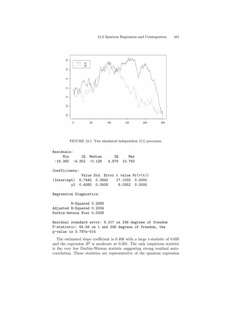
Following Granger and Newbold (1974), 250 observations for each seriesare simulated and plotted in Figure 12.1 using
> set.seed(458)
> e1 = rnorm(250)
> e2 = rnorm(250)
> y1 = cumsum(e1)
> y2 = cumsum(e2)
> tsplot(y1, y2, lty=c(1,3))
> legend(0, 15, c("y1","y2"), lty=c(1,3))
The data in the graph resemble stock prices or exchange rates. A visualinspection of the data suggests that the levels of the two series are positivelyrelated. Regressing y1t on y2t reinforces this observation:
> summary(OLS(y1~y2))
Call:
OLS(formula = y1 ~y2)
1A systematic technical analysis of the linear regression model with I(1) and I(0) vari-ables is given in Sims, Stock and Watson (1990). Hamilton (1994) gives a nice summaryof these results and Stock and Watson (1989) provides useful intuition and examples.
12.2 Spurious Regression and Cointegration 431
0 50 100 150 200 250
-15
-10
-50
510
15y1y2
FIGURE 12.1. Two simulated independent I(1) processes.
Residuals:
Min 1Q Median 3Q Max
-16.360 -4.352 -0.128 4.979 10.763
Coefficients:
Value Std. Error t value Pr(>|t|)
(Intercept) 6.7445 0.3943 17.1033 0.0000
y2 0.4083 0.0508 8.0352 0.0000
Regression Diagnostics:
R-Squared 0.2066
Adjusted R-Squared 0.2034
Durbin-Watson Stat 0.0328
Residual standard error: 6.217 on 248 degrees of freedom
F-statistic: 64.56 on 1 and 248 degrees of freedom, the
p-value is 3.797e-014
The estimated slope coefficient is 0.408 with a large t-statistic of 8.035and the regression R2 is moderate at 0.201. The only suspicious statisticis the very low Durbin-Watson statistic suggesting strong residual auto-correlation. These statistics are representative of the spurious regression

432 12. Cointegration
phenomenon with I(1) that are not cointegrated. If ∆y1t is regressed on∆y2t the correct relationship between the two series is revealed
> summary(OLS(diff(y1)~diff(y2)))
Call:
OLS(formula = diff(y1) ~diff(y2))
Residuals:
Min 1Q Median 3Q Max
-3.6632 -0.7706 -0.0074 0.6983 2.7184
Coefficients:
Value Std. Error t value Pr(>|t|)
(Intercept) -0.0565 0.0669 -0.8447 0.3991
diff(y2) 0.0275 0.0642 0.4290 0.6683
Regression Diagnostics:
R-Squared 0.0007
Adjusted R-Squared -0.0033
Durbin-Watson Stat 1.9356
Residual standard error: 1.055 on 247 degrees of freedom
F-statistic: 0.184 on 1 and 247 degrees of freedom, the
p-value is 0.6683
Similar results to those above occur if cov(ε1t, ε2t) 6= 0. The levels re-gression remains spurious (no real long-run common movement in levels),but the differences regression will reflect the non-zero contemporaneouscorrelation between ∆y1t and ∆y2t.
Statistical Implications of Spurious Regression
Let Yt = (y1t, . . . , ynt)0 denote an (n×1) vector of I(1) time series that are
not cointegrated. Using the partition Yt = (y1t,Y02t)
0, consider the leastsquares regression of y1t on Y2t giving the fitted model
y1t = β02Y2t + ut (12.1)
Since y1t is not cointegrated with Y2t (12.1) is a spurious regression andthe true value of β2 is zero. The following results about the behavior of β2in the spurious regression (12.1) are due to Phillips (1986):
• β2 does not converge in probability to zero but instead converges indistribution to a non-normal random variable not necessarily centeredat zero. This is the spurious regression phenomenon.

12.2 Spurious Regression and Cointegration 433
• The usual OLS t-statistics for testing that the elements of β2 are zerodiverge to ±∞ as T →∞. Hence, with a large enough sample it willappear that Yt is cointegrated when it is not if the usual asymptoticnormal inference is used.
• The usual R2 from the regression converges to unity as T → ∞ sothat the model will appear to fit well even though it is misspecified.
• Regression with I(1) data only makes sense when the data are coin-tegrated.
12.2.2 Cointegration
Let Yt = (y1t, . . . , ynt)0 denote an (n× 1) vector of I(1) time series. Yt is
cointegrated if there exists an (n× 1) vector β = (β1, . . . , βn)0 such that
β0Yt = β1y1t + · · ·+ βnynt ∼ I(0) (12.2)
In words, the nonstationary time series in Yt are cointegrated if there isa linear combination of them that is stationary or I(0). If some elementsof β are equal to zero then only the subset of the time series in Yt withnon-zero coefficients is cointegrated. The linear combination β0Yt is oftenmotivated by economic theory and referred to as a long-run equilibriumrelationship. The intuition is that I(1) time series with a long-run equilib-rium relationship cannot drift too far apart from the equilibrium becauseeconomic forces will act to restore the equilibrium relationship.
Normalization
The cointegration vector β in (12.2) is not unique since for any scalar cthe linear combination cβ0Yt = β∗0Yt ∼ I(0). Hence, some normalizationassumption is required to uniquely identify β. A typical normalization is
β = (1,−β2, . . . ,−βn)0
so that the cointegration relationship may be expressed as
β0Yt = y1t − β2y2t − · · ·− βnynt ∼ I(0)
ory1t = β2y2t + · · ·+ βnynt + ut (12.3)
where ut ∼ I(0). In (12.3), the error term ut is often referred to as thedisequilibrium error or the cointegrating residual. In long-run equilibrium,the disequilibrium error ut is zero and the long-run equilibrium relationshipis
y1t = β2y2t + · · ·+ βnynt

434 12. Cointegration
Multiple Cointegrating Relationships
If the (n×1) vectorYt is cointegrated there may be 0 < r < n linearly inde-pendent cointegrating vectors. For example, let n = 3 and suppose there arer = 2 cointegrating vectors β1 = (β11, β12, β13)
0 and β2 = (β21, β22, β23)0.Then β01Yt = β11y1t + β12y2t + β13y3t ∼ I(0), β02Yt = β21y1t + β22y2t +β23y3t ∼ I(0) and the (3× 2) matrix
B0 =µβ01β02
¶=
µβ11 β12 β13β21 β22 β33
¶forms a basis for the space of cointegrating vectors. The linearly indepen-dent vectors β1 and β2 in the cointegrating basis B are not unique unlesssome normalization assumptions are made. Furthermore, any linear combi-nation of β1 and β2, e.g. β3 = c1β1 + c2β2 where c1 and c2 are constants,is also a cointegrating vector.
Examples of Cointegration and Common Trends in Economics andFinance
Cointegration naturally arises in economics and finance. In economics, coin-tegration is most often associated with economic theories that imply equi-librium relationships between time series variables. The permanent incomemodel implies cointegration between consumption and income, with con-sumption being the common trend. Money demand models imply cointe-gration between money, income, prices and interest rates. Growth theorymodels imply cointegration between income, consumption and investment,with productivity being the common trend. Purchasing power parity im-plies cointegration between the nominal exchange rate and foreign anddomestic prices. Covered interest rate parity implies cointegration betweenforward and spot exchange rates. The Fisher equation implies cointegrationbetween nominal interest rates and inflation. The expectations hypothesisof the term structure implies cointegration between nominal interest ratesat different maturities. The equilibrium relationships implied by these eco-nomic theories are referred to as long-run equilibrium relationships, becausethe economic forces that act in response to deviations from equilibriiummay take a long time to restore equilibrium. As a result, cointegrationis modeled using long spans of low frequency time series data measuredmonthly, quarterly or annually.In finance, cointegration may be a high frequency relationship or a low
frequency relationship. Cointegration at a high frequency is motivated byarbitrage arguments. The Law of One Price implies that identical assetsmust sell for the same price to avoid arbitrage opportunities. This impliescointegration between the prices of the same asset trading on differentmarkets, for example. Similar arbitrage arguments imply cointegration be-tween spot and futures prices, and spot and forward prices, and bid and

12.2 Spurious Regression and Cointegration 435
ask prices. Here the terminology long-run equilibrium relationship is some-what misleading because the economic forces acting to eliminate arbitrageopportunities work very quickly. Cointegration is appropriately modeledusing short spans of high frequency data in seconds, minutes, hours ordays. Cointegration at a low frequency is motivated by economic equilib-rium theories linking assets prices or expected returns to fundamentals. Forexample, the present value model of stock prices states that a stock’s priceis an expected discounted present value of its expected future dividends orearnings. This links the behavior of stock prices at low frequencies to thebehavior of dividends or earnings. In this case, cointegration is modeledusing low frequency data and is used to explain the long-run behavior ofstock prices or expected returns.
12.2.3 Cointegration and Common Trends
If the (n × 1) vector time series Yt is cointegrated with 0 < r < n coin-tegrating vectors then there are n − r common I(1) stochastic trends.To illustrate the duality between cointegration and common trends, letYt = (y1t, y2t)
0 ∼ I(1) and εt = (ε1t, ε2t, ε3t)0 ∼ I(0) and suppose that Yt
is cointegrated with cointegrating vector β = (1,−β2)0. This cointegrationrelationship may be represented as
y1t = β2
tXs=1
ε1s + ε3t
y2t =tX
s=1
ε1s + ε2t
The common stochastic trend isPt
s=1 ε1s. Notice that the cointegratingrelationship annihilates the common stochastic trend:
β0Yt = β2
tXs=1
ε1s + ε3t − β2
ÃtX
s=1
ε1s + ε2t
!= ε3t − β2ε2t ∼ I(0).
12.2.4 Simulating Cointegrated Systems
Cointegrated systems may be conveniently simulated using Phillips’ (1991)triangular representation. For example, consider a bivariate cointegratedsystem for Yt = (y1t, y2t)
0 with cointegrating vector β = (1,−β2)0. Atriangular representation has the form
y1t = β2y2t + ut, where ut ∼ I(0) (12.4)
y2t = y2t−1 + vt, where vt ∼ I(0) (12.5)
436 12. Cointegration
The first equation describes the long-run equilibrium relationship with anI(0) disequilibrium error ut. The second equation specifies y2t as the com-mon stochastic trend with innovation vt:
y2t = y20 +tX
j=1
vj .
In general, the innovations ut and vt may be contemporaneously and seriallycorrelated. The time series structure of these innovations characterizes theshort-run dynamics of the cointegrated system. The system (12.4)-(12.5)with β2 = 1, for example, might be used to model the behavior of thelogarithm of spot and forward prices, spot and futures prices or stock pricesand dividends.
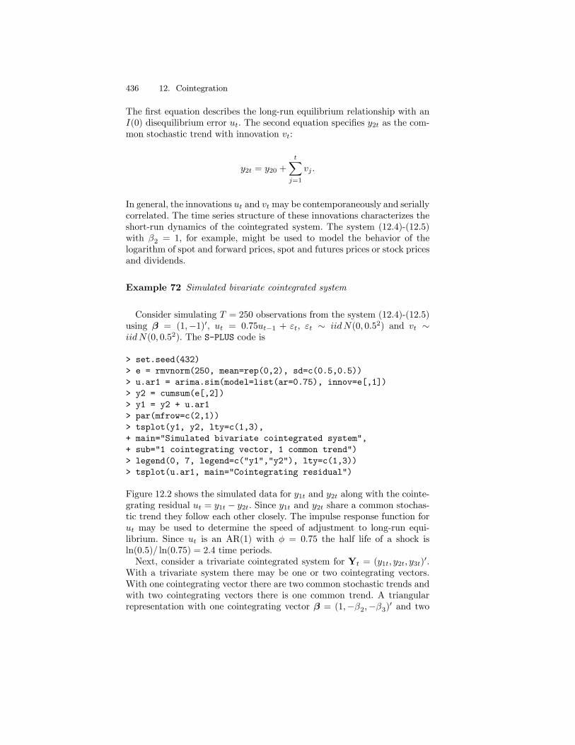
Example 72 Simulated bivariate cointegrated system
Consider simulating T = 250 observations from the system (12.4)-(12.5)using β = (1,−1)0, ut = 0.75ut−1 + εt, εt ∼ iidN(0, 0.52) and vt ∼iidN(0, 0.52). The S-PLUS code is
> set.seed(432)
> e = rmvnorm(250, mean=rep(0,2), sd=c(0.5,0.5))
> u.ar1 = arima.sim(model=list(ar=0.75), innov=e[,1])
> y2 = cumsum(e[,2])
> y1 = y2 + u.ar1
> par(mfrow=c(2,1))
> tsplot(y1, y2, lty=c(1,3),
+ main="Simulated bivariate cointegrated system",
+ sub="1 cointegrating vector, 1 common trend")
> legend(0, 7, legend=c("y1","y2"), lty=c(1,3))
> tsplot(u.ar1, main="Cointegrating residual")
Figure 12.2 shows the simulated data for y1t and y2t along with the cointe-grating residual ut = y1t − y2t. Since y1t and y2t share a common stochas-tic trend they follow each other closely. The impulse response function forut may be used to determine the speed of adjustment to long-run equi-librium. Since ut is an AR(1) with φ = 0.75 the half life of a shock isln(0.5)/ ln(0.75) = 2.4 time periods.Next, consider a trivariate cointegrated system for Yt = (y1t, y2t, y3t)
0.With a trivariate system there may be one or two cointegrating vectors.With one cointegrating vector there are two common stochastic trends andwith two cointegrating vectors there is one common trend. A triangularrepresentation with one cointegrating vector β = (1,−β2,−β3)0 and two

12.2 Spurious Regression and Cointegration 437
Simulated bivariate cointegrated system
1 cointegrating vector, 1 common trend
0 50 100 150 200 250
-20
24
68
y1y2
Cointegrating residual
0 50 100 150 200 250
-10
12
FIGURE 12.2. Simulated bivariate cointegrated system with β = (1,−1)0.
stochastic trends is
y1t = β2y2t + β3y3t + ut, where ut ∼ I(0) (12.6)
y2t = y2t−1 + vt, where vt ∼ I(0) (12.7)
y3t = y3t−1 + wt, where wt ∼ I(0) (12.8)
The first equation describes the long-run equilibrium and the second andthird equations specify the common stochastic trends. An example of atrivariate cointegrated system with one cointegrating vector is a system ofnominal exchange rates, home country price indices and foreign countryprice indices. A cointegrating vector β = (1,−1,−1)0 implies that the realexchange rate is stationary.
Example 73 Simulated trivariate cointegrated system with 1 cointegratingvector
The S-PLUS code for simulating T = 250 observation from (12.6)-(12.8)with β = (1,−0.5,−0.5)0, ut = 0.75ut−1 + εt, εt ∼ iidN(0, 0.52), vt ∼iidN(0, 0.52) and wt ∼ iidN(0, 0.52) is
> set.seed(573)
> e = rmvnorm(250, mean=rep(0,3), sd=c(0.5,0.5,0.5))
> u1.ar1 = arima.sim(model=list(ar=0.75), innov=e[,1])
> y2 = cumsum(e[,2])
438 12. Cointegration
Simulated trivariate cointegrated system
1 cointegrating vector, 2 common trends
0 50 100 150 200 250
05
10
y1y2y3
Cointegrating residual
0 50 100 150 200 250
-10
12
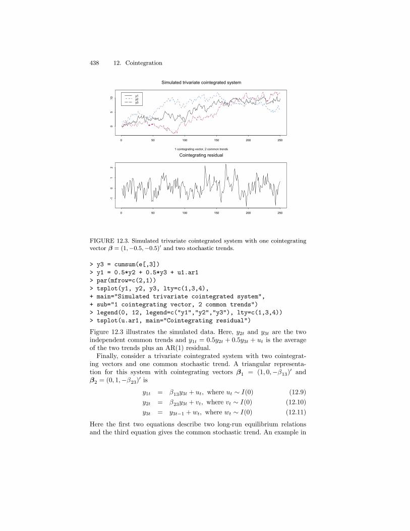
FIGURE 12.3. Simulated trivariate cointegrated system with one cointegratingvector β = (1,−0.5,−0.5)0 and two stochastic trends.
> y3 = cumsum(e[,3])
> y1 = 0.5*y2 + 0.5*y3 + u1.ar1
> par(mfrow=c(2,1))
> tsplot(y1, y2, y3, lty=c(1,3,4),
+ main="Simulated trivariate cointegrated system",
+ sub="1 cointegrating vector, 2 common trends")
> legend(0, 12, legend=c("y1","y2","y3"), lty=c(1,3,4))
> tsplot(u.ar1, main="Cointegrating residual")
Figure 12.3 illustrates the simulated data. Here, y2t and y3t are the twoindependent common trends and y1t = 0.5y2t + 0.5y3t + ut is the averageof the two trends plus an AR(1) residual.Finally, consider a trivariate cointegrated system with two cointegrat-
ing vectors and one common stochastic trend. A triangular representa-tion for this system with cointegrating vectors β1 = (1, 0,−β13)0 andβ2 = (0, 1,−β23)0 is
y1t = β13y3t + ut, where ut ∼ I(0) (12.9)
y2t = β23y3t + vt, where vt ∼ I(0) (12.10)
y3t = y3t−1 + wt, where wt ∼ I(0) (12.11)
Here the first two equations describe two long-run equilibrium relationsand the third equation gives the common stochastic trend. An example in

12.2 Spurious Regression and Cointegration 439
finance of such a system is the term structure of interest rates where y3represents the short rate and y1 and y2 represent two different long rates.The cointegrating relationships would indicate that the spreads betweenthe long and short rates are stationary.
Example 74 Simulated trivariate cointegrated system with 2 cointegratingvectors
The S-PLUS code for simulating T = 250 observation from (12.9)-(12.11)with β1 = (1, 0,−1)0, β2 = (0, 1,−1)0, ut = 0.75ut−1+εt, εt ∼ iidN(0, 0.52),vt = 0.75vt−1 + ηt, ηt ∼ iidN(0, 0.52) and wt ∼ iidN(0, 0.52) is
> set.seed(573)
> e = rmvnorm(250,mean=rep(0,3), sd=c(0.5,0.5,0.5))
> u.ar1 = arima.sim(model=list(ar=0.75), innov=e[,1])
> v.ar1 = arima.sim(model=list(ar=0.75), innov=e[,2])
> y3 = cumsum(e[,3])
> y1 = y3 + u.ar1
> y2 = y3 + v.ar1
> par(mfrow=c(2,1))
> tsplot(y1, y2, y3, lty=c(1,3,4),
+ main="Simulated trivariate cointegrated system",
+ sub="2 cointegrating vectors, 1 common trend")
> legend(0, 10, legend=c("y1","y2","y3"), lty=c(1,3,4))
> tsplot(u.ar1, v.ar1, lty=c(1,3),
+ main="Cointegrated residuals")
> legend(0, -1, legend=c("u","v"), lty=c(1,3))
12.2.5 Cointegration and Error Correction Models
Consider a bivariate I(1) vector Yt = (y1t, y2t)0 and assume that Yt is
cointegrated with cointegrating vector β = (1,−β2)0 so that β0Yt = y1t −β2y2t is I(0). In an extremely influential and important paper, Engle andGranger (1987) showed that cointegration implies the existence of an errorcorrection model (ECM) of the form
∆y1t = c1 + α1(y1t−1 − β2y2t−1) (12.12)
+Xj
ψj11∆y1t−j +Xj
ψj12∆y2t−j + ε1t
∆y2t = c2 + α2(y1t−1 − β2y2t−1) (12.13)
+Xj
ψj21∆y1t−j +Xj
ψ222∆y2t−j + ε2t
that describes the dynamic behavior of y1t and y2t. The ECM links thelong-run equilibrium relationship implied by cointegration with the short-run dynamic adjustment mechanism that describes how the variables react

440 12. Cointegration
Simulated trivariate cointegrated system
2 cointegrating vectors, 1 common trend
0 50 100 150 200 250
05
10
y1y2y3
Cointegrated residuals
0 50 100 150 200 250
-2-1
01
uv
FIGURE 12.4. Simulated trivatiate cointegrated system with two cointegratingvectors β1 = (1, 0,−1)0, β2 = (0, 1,−1)0 and one common trend.
when they move out of long-run equilibrium. This ECM makes the conceptof cointegration useful for modeling financial time series.
Example 75 Bivariate ECM for stock prices and dividends
As an example of an ECM, let st denote the log of stock prices and dtdenote the log of dividends and assume that Yt = (st, dt)
0 is I(1). If thelog dividend-price ratio is I(0) then the logs of stock prices and dividendsare cointegrated with β = (1,−1)0. That is, the long-run equilibrium is
dt = st + µ+ ut
where µ is the mean of the log dividend-price ratio, and ut is an I(0) randomvariable representing the dynamic behavior of the log dividend-price ratio(disequilibrium error). Suppose the ECM has the form
∆st = cs + αs(dt−1 − st−1 − µ) + εst
∆dt = cd + αd(dt−1 − st−1 − µ) + εdt
where cs > 0 and cd > 0. The first equation relates the growth rate ofdividends to the lagged disequilibrium error dt−1−st−1−µ, and the secondequation relates the growth rate of stock prices to the lagged disequilibriumas well. The reactions of st and dt to the disequilibrium error are capturedby the adjustment coefficients αs and αd.
12.2 Spurious Regression and Cointegration 441
Consider the special case of (12.12)-(12.13) where αd = 0 and αs = 0.5.The ECM equations become
∆st = cs + 0.5(dt−1 − st−1 − µ) + εst,
∆dt = cd + εdt.
so that only st responds to the lagged disequilibrium error. Notice thatE[∆st|Yt−1] = cs + 0.5(dt−1 − st−1 − µ) and E[∆dt|Yt−1] = cd. Considerthree situations:
1. dt−1−st−1−µ = 0. Then E[∆st|Yt−1] = cs and E[∆dt|Yt−1] = cd, sothat cs and cd represent the growth rates of stock prices and dividendsin long-run equilibrium.
2. dt−1− st−1−µ > 0. Then E[∆st|Yt−1] = cs+0.5(dt−1− st−1−µ) >cs. Here the dividend yield has increased above its long-run mean(positive disequilibrium error) and the ECM predicts that st will growfaster than its long-run rate to restore the dividend yield to its long-run mean. Notice that the magnitude of the adjustment coefficientαs = 0.5 controls the speed at which st responds to the disequilibriumerror.
3. dt−1− st−1−µ < 0. Then E[∆st|Yt−1] = cs+0.5(dt−1− st−1−µ) <cs. Here the dividend yield has decreased below its long-run mean(negative disequilibrium error) and the ECM predicts that st willgrow more slowly than its long-run rate to restore the dividend yieldto its long-run mean.
In Case 1, there is no expected adjustment since the model was in long-run equilibrium in the previous period. In Case 2, the model was abovelong-run equilibrium last period so the expected adjustment in st is down-ward toward equilibrium. In Case 3, the model was below long-run equi-librium last period and so the expected adjustment is upward toward theequilibrium. This discussion illustrates why the model is called an error cor-rection model. When the variables are out of long-run equilibrium, thereare economic forces, captured by the adjustment coefficients, that pushthe model back to long-run equilibrium. The speed of adjustment towardequilibrium is determined by the magnitude of αs. In the present example,αs = 0.5 which implies that roughly one half of the disequilibrium erroris corrected in one time period. If αs = 1 then the entire disequilibriumis corrected in one period. If αs = 1.5 then the correction overshoots thelong-run equilibrium.

442 12. Cointegration
12.3 Residual-Based Tests for Cointegration
Let the (n×1) vector Yt be I(1). Recall, Yt is cointegrated with 0 < r < ncointegrating vectors if there exists an (r × n) matrix B0 such that
B0Yt =
β01Yt
...β0rYt
=
u1t...urt
∼ I(0)
Testing for cointegration may be thought of as testing for the existenceof long-run equilibria among the elements of Yt. Cointegration tests covertwo situations:
• There is at most one cointegrating vector• There are possibly 0 ≤ r < n cointegrating vectors.
The first case was originally considered by Engle and Granger (1986) andthey developed a simple two-step residual-based testing procedure basedon regression techniques. The second case was originally considered by Jo-hansen (1988) who developed a sophisticated sequential procedure for de-termining the existence of cointegration and for determining the number ofcointegrating relationships based on maximum likelihood techniques. Thissection explains Engle and Granger’s two-step procedure. Johansen’s moregeneral procedure will be discussed later on.Engle and Granger’s two-step procedure for determining if the (n × 1)
vector β is a cointegrating vector is as follows:
• Form the cointegrating residual β0Yt = ut
• Perform a unit root test on ut to determine if it is I(0).
The null hypothesis in the Engle-Granger procedure is no-cointegration andthe alternative is cointegration. There are two cases to consider. In the firstcase, the proposed cointegrating vector β is pre-specified (not estimated).For example, economic theory may imply specific values for the elementsin β such as β = (1,−1)0. The cointegrating residual is then readily con-structed using the prespecified cointegrating vector. In the second case, theproposed cointegrating vector is estimated from the data and an estimate
of the cointegrating residual β0Yt = ut is formed. Tests for cointegration
using a pre-specified cointegrating vector are generally much more powerfulthan tests employing an estimated vector.
12.3.1 Testing for Cointegration When the CointegratingVector Is Pre-specified
Let Yt denote an (n× 1) vector of I(1) time series, let β denote an (n× 1)prespecified cointegrating vector and let ut = β0Yt denote the prespecified
12.3 Residual-Based Tests for Cointegration 443
Log US/CA exchange rate data
1976 1977 1978 1979 1980 1981 1982 1983 1984 1985 1986 1987 1988 1989 1990 1991 1992 1993 1994 1995 1996
-0.3
5-0
.15
0.00
spotforward
US/CA 30-day interest rate differential
1976 1977 1978 1979 1980 1981 1982 1983 1984 1985 1986 1987 1988 1989 1990 1991 1992 1993 1994 1995 1996
-0.0
040.
000
0.00
4
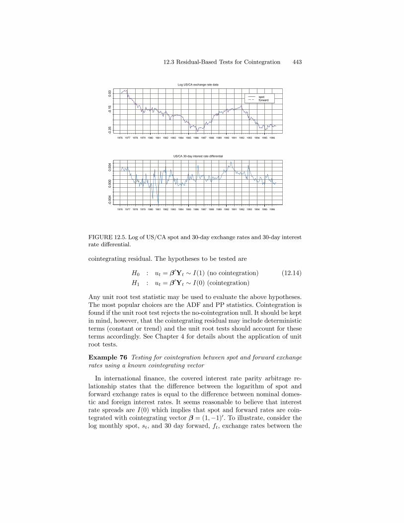
FIGURE 12.5. Log of US/CA spot and 30-day exchange rates and 30-day interestrate differential.
cointegrating residual. The hypotheses to be tested are
H0 : ut = β0Yt ∼ I(1) (no cointegration) (12.14)
H1 : ut = β0Yt ∼ I(0) (cointegration)
Any unit root test statistic may be used to evaluate the above hypotheses.The most popular choices are the ADF and PP statistics. Cointegration isfound if the unit root test rejects the no-cointegration null. It should be keptin mind, however, that the cointegrating residual may include deterministicterms (constant or trend) and the unit root tests should account for theseterms accordingly. See Chapter 4 for details about the application of unitroot tests.
Example 76 Testing for cointegration between spot and forward exchangerates using a known cointegrating vector
In international finance, the covered interest rate parity arbitrage re-lationship states that the difference between the logarithm of spot andforward exchange rates is equal to the difference between nominal domes-tic and foreign interest rates. It seems reasonable to believe that interestrate spreads are I(0) which implies that spot and forward rates are coin-tegrated with cointegrating vector β = (1,−1)0. To illustrate, consider thelog monthly spot, st, and 30 day forward, ft, exchange rates between the

444 12. Cointegration
US and Canada over the period February 1976 through June 1996 takenfrom the S+FinMetrics “timeSeries” object lexrates.dat
> uscn.s = lexrates.dat[,"USCNS"]
> uscn.s@title = "Log of US/CA spot exchange rate"
> uscn.f = lexrates.dat[,"USCNF"]
> uscn.f@title = "Log of US/CA 30-day forward exchange rate"
> u = uscn.s - uscn.f
> colIds(u) = "USCNID"
> u@title = "US/CA 30-day interest rate differential"
The interest rate differential is constructed using the pre-specified cointe-grating vector β = (1,−1)0 as ut = st−ft. The spot and forward exchangerates and interest rate differential are illustrated in Figure 12.5. Visually,the spot and forward exchange rates clearly share a common trend and theinterest rate differential appears to be I(0). In addition, there is no clear de-terministic trend behavior in the exchange rates. The S+FinMetrics func-tion unitroot may be used to test the null hypothesis that st and ft arenot cointegrated (ut ∼ I(1)). The ADF t-test based on 11 lags and a con-stant in the test regression leads to the rejection at the 5% level of thehypothesis that st and ft are not cointegrated with cointegrating vectorβ = (1,−1)0:
> unitroot(u, trend="c", method="adf", lags=11)
Test for Unit Root: Augmented DF Test
Null Hypothesis: there is a unit root
Type of Test: t-test
Test Statistic: -2.881
P-value: 0.04914
Coefficients:
lag1 lag2 lag3 lag4 lag5 lag6 lag7
-0.1464 -0.1171 -0.0702 -0.1008 -0.1234 -0.1940 0.0128
lag8 lag9 lag10 lag11 constant
-0.1235 0.0550 0.2106 -0.1382 0.0002
Degrees of freedom: 234 total; 222 residual
Time period: from Jan 1977 to Jun 1996
Residual standard error: 8.595e-4
12.3 Residual-Based Tests for Cointegration 445
12.3.2 Testing for Cointegration When the CointegratingVector Is Estimated
Let Yt denote an (n × 1) vector of I(1) time series and let β denote an(n × 1) unknown cointegrating vector. The hypotheses to be tested aregiven in (12.14). Since β is unknown, to use the Engle-Granger procedureit must be first estimated from the data. Before β can be estimated somenormalization assumption must be made to uniquely identify it. A commonnormalization is to specify the first element inYt as the dependent variableand the rest as the explanatory variables. Then Yt = (y1t,Y
02t)
0 whereY2t = (y2t, . . . , ynt)
0 is an ((n− 1)× 1) vector and the cointegrating vectoris normalized as β = (1,−β02)0. Engle and Granger propose estimating thenormalized cointegrating vector β2 by least squares from the regression
y1t = c+ β02Y2t + ut (12.15)
and testing the no-cointegration hypothesis (12.14) with a unit root testusing the estimated cointegrating residual
ut = y1t − c− β2Y2t (12.16)
where c and β2 are the least squares estimates of c and β2. The unit roottest regression in this case is without deterministic terms (constant or con-stant and trend). Phillips and Ouliaris (1990) show that ADF and PP unitroot tests (t-tests and normalized bias) applied to the estimated cointegrat-ing residual (12.16) do not have the usual Dickey-Fuller distributions underthe null hypothesis (12.14) of no-cointegration. Instead, due to the spuriousregression phenomenon under the null hypothesis (12.14), the distributionof the ADF and PP unit root tests have asymptotic distributions that arefunctions of Wiener processes that depend on the deterministic terms inthe regression (12.15) used to estimate β2 and the number of variables,n− 1, in Y2t. These distributions are known as the Phillips-Ouliaris (PO)distributions, and are described in Phillips and Ouliaris (1990). To furthercomplicate matters, Hansen (1992) showed the appropriate PO distribu-tions of the ADF and PP unit root tests applied to the residuals (12.16)also depend on the trend behavior of y1t and Y2t as follows:
Case I: Y2t and y1t are both I(1) without drift. The ADF and PP unitroot test statistics follow the PO distributions, adjusted for a con-stant, with dimension parameter n− 1.
Case II: Y2t is I(1) with drift and y1t may or may not be I(1) with drift.The ADF and PP unit root test statistics follow the PO distributions,adjusted for a constant and trend, with dimension parameter n− 2.If n− 2 = 0 then the ADF and PP unit root test statistics follow theDF distributions adjusted for a constant and trend.

446 12. Cointegration
Case III: Y2t is I(1) without drift and y1t is I(1) with drift. In this case,β2 should be estimated from the regression
y1t = c+ δt+ β02Y2t + ut (12.17)
The resulting ADF and PP unit root test statistics on the residualsfrom (12.17) follow the PO distributions, adjusted for a constant andtrend, with dimension parameter n− 1.
Computing Quantiles and P-values from the Phillips-OuliarisDistributions Using the S+FinMetrics Functions pcoint and qcoint
The S+FinMetrics functions qcoint and pcoint, based on the responsesurface methodology of MacKinnon (1996), may be used to compute quan-tiles and p-values from the PO distributions. For example, to compute the10%, 5% and 1% quantiles from the PO distribution for the ADF t-statistic,adjusted for a constant, with n− 1 = 3 and a sample size T = 100 use> qcoint(c(0.1,0.05,0.01), n.sample=100, n.series=4,
+ trend="c", statistic="t")
[1] -3.8945 -4.2095 -4.8274
Notice that the argument n.series represents the total number of variablesn. To adjust the PO distributions for a constant and trend set trend="ct".To compute the PO distribution for the ADF normalized bias statisticset statistic="n". The quantiles from the PO distributions can be verydifferent from the quantiles from the DF distributions, especially if n−1 islarge. To illustrate, the 10%, 5% and 1% quantiles from the DF distributionfor the ADF t-statistic with a sample size T = 100 are
> qunitroot(c(0.1,0.05,0.01), n.sample=100,
+ trend="c", statistic="t")
[1] -2.5824 -2.8906 -3.4970
The following examples illustrate testing for cointegration using an esti-mated cointegrating vector.
Example 77 Testing for cointegration between spot and forward exchangerates using an estimated cointegrating vector
Consider testing for cointegration between spot and forward exchangerates assuming the cointegrating vector is not known using the same data asin the previous example. Let Yt = (st, ft)
0 and normalize the cointegratingvector on st so that β = (1,−β2)0. The normalized cointegrating coefficientβ2 is estimated by least squares from the regression
st = c+ β2ft + ut
giving the estimated cointegrating residual ut = st − c − β2ft. The OLSfunction in S+FinMetrics is used to estimate the above regression:
12.3 Residual-Based Tests for Cointegration 447
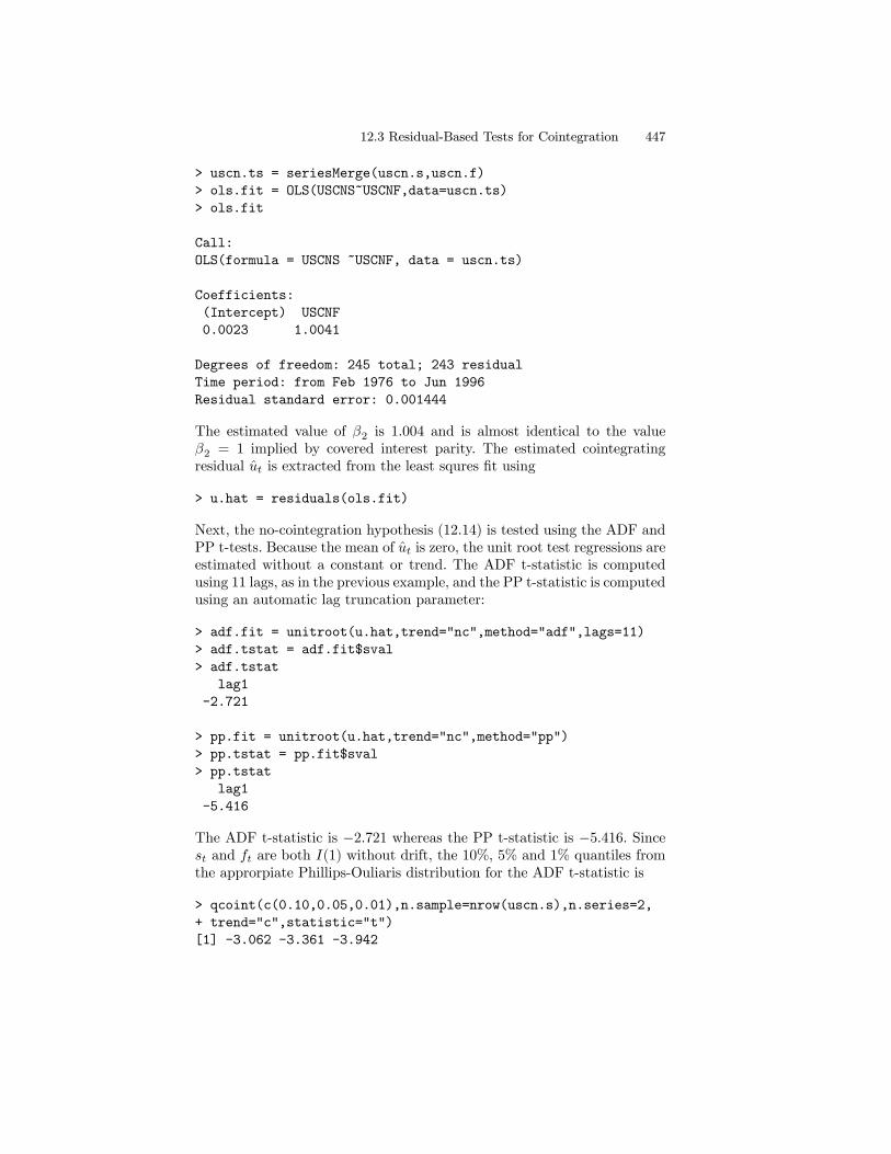
> uscn.ts = seriesMerge(uscn.s,uscn.f)
> ols.fit = OLS(USCNS~USCNF,data=uscn.ts)
> ols.fit
Call:
OLS(formula = USCNS ~USCNF, data = uscn.ts)
Coefficients:
(Intercept) USCNF
0.0023 1.0041
Degrees of freedom: 245 total; 243 residual
Time period: from Feb 1976 to Jun 1996
Residual standard error: 0.001444
The estimated value of β2 is 1.004 and is almost identical to the valueβ2 = 1 implied by covered interest parity. The estimated cointegratingresidual ut is extracted from the least squres fit using
> u.hat = residuals(ols.fit)
Next, the no-cointegration hypothesis (12.14) is tested using the ADF andPP t-tests. Because the mean of ut is zero, the unit root test regressions areestimated without a constant or trend. The ADF t-statistic is computedusing 11 lags, as in the previous example, and the PP t-statistic is computedusing an automatic lag truncation parameter:
> adf.fit = unitroot(u.hat,trend="nc",method="adf",lags=11)
> adf.tstat = adf.fit$sval
> adf.tstat
lag1
-2.721
> pp.fit = unitroot(u.hat,trend="nc",method="pp")
> pp.tstat = pp.fit$sval
> pp.tstat
lag1
-5.416
The ADF t-statistic is −2.721 whereas the PP t-statistic is −5.416. Sincest and ft are both I(1) without drift, the 10%, 5% and 1% quantiles fromthe approrpiate Phillips-Ouliaris distribution for the ADF t-statistic is
> qcoint(c(0.10,0.05,0.01),n.sample=nrow(uscn.s),n.series=2,
+ trend="c",statistic="t")
[1] -3.062 -3.361 -3.942

448 12. Cointegration
The no-cointegration null hypothesis is not rejected at the 10% level usingthe ADF t-statistic but is rejected at the 1% level using the PP t-statistic.The p-values for the ADF and PP t-statistics are
> pcoint(adf.tstat, n.sample=nrow(uscn.s), n.series=2,
+ trend="c", statistic="t")
[1] 0.1957
> pcoint(pp.tstat, n.sample=nrow(uscn.s), n.series=2,
+ trend="c", statistic="t")
[1] 0.00003925
12.4 Regression-Based Estimates of CointegratingVectors and Error Correction Models
12.4.1 Least Square Estimator
Least squares may be used to consistently estimate a normalized cointe-grating vector. However, the asymptotic behavior of the least squares es-timator is non-standard. The following results about the behavior of β2 ifYt is cointegrated are due to Stock (1987) and Phillips (1991):
• T (β2−β2) converges in distribution to a non-normal random variablenot necessarily centered at zero.
• The least squares estimate β2 is consistent for β2 and converges toβ2 at rate T instead of the usual rate T 1/2. That is, β2 is superconsistent.
• β2 is consistent even if Y2t is correlated with ut so that there is noasymptotic simultaneity bias.
• In general, the asymptotic distribution of T (β2 − β2) is asymptoti-cally biased and non-normal. The usual OLS formula for computing[avar(β2) is incorrect and so the usual OLS standard errors are notcorrect.
• Even though the asymptotic bias goes to zero as T gets large β2 maybe substantially biased in small samples. The least squres estimatoris also not efficient.
The above results indicate that the least squares estimator of the coin-tegrating vector β2 could be improved upon. A simple improvement issuggested by Stock and Watson (1993).

12.4 Regression-Based Estimates and Error Correction Models 449
12.4.2 Stock and Watson’s Efficient Lead/Lag Estimator
Stock and Watson (1993) provide a very simple method for obtaining anasymptotically efficient (equivalent to maximum likelihood) estimator forthe normalized cointegrating vector β2 as well as a valid formula for com-puting its asymptotic variance2.Let Yt = (y1t,Y
02t)
0 where Y2t = (y2t, . . . , ynt)0 is an ((n−1)×1) vector
and let the cointegrating vector be normalized as β = (1,−β02)0. Stock andWatson’s efficient estimation procedure is:
• Augment the cointegrating regression of y1t on Y2t with appropriatedeterministic terms Dt with p leads and lags of ∆Y2t
y1t = γ0Dt + β02Y2t +
pXj=−p
ψ0j∆Y2t−j + ut (12.18)
= γ0Dt + β02Y2t +ψ0p∆Y2t+p + · · ·+ψ01∆Y2t+1
+ψ00∆Y2t +ψ0−1∆Y2t−1 + · · ·+ψ0−p∆Y2t−p + ut
• Estimate the augmented regression by least squares. The resultingestimator of β2 is called the dynamic OLS estimator and is denotedβ2,DOLS . It will be consistent, asymptotically normally distributedand efficient (equivalent to MLE) under certain assumptions (seeStock and Watson, 1993).
• Asymptotically valid standard errors for the individual elements ofβ2,DOLS are given by the OLS standard errors from (12.18) multipliedby the ratio Ã
σ2uclrv(ut)!1/2
where σ2u is the OLS estimate of var(ut) andclrv(ut) is any consistent
estimate of the long-run variance of ut using the residuals ut from(12.18). Alternatively, the Newey-West HAC standard errors may alsobe used.
Example 78 DOLS estimation of cointegrating vector using exchange ratedata3
Let st denote the log of the monthly spot exchange rate between twocurrencies at time t and let fkt denote the log of the forward exchangerate at time t for delivery of foreign currency at time t+ k. Under rational
2Hamilton (1994) chapter 19, and Hayashi (2000) chapter 10, give nice discussions ofthe Stock and Watson procedure.
3This example is based on Zivot (2000).

450 12. Cointegration
expectations and risk neutrality fkt is an unbiased predictor of st+k, thespot exchange rate at time t+ k. That is
st+k = fkt + εt+k
where εt+k is a white noise error term. This is known as the forwardrate unbiasedness hypothesis (FRUH). Assuming that st and fkt are I(1)the FRUH implies that st+k and fkt are cointegrated with cointegrat-ing vector β = (1,−1)0. To illustrate, consider again the log monthlyspot, st, and one month forward, f
1t , exchange rates between the US and
Canada over the period February 1976 through June 1996 taken from theS+FinMetrics “timeSeries” object lexrates.dat.The cointegrating vec-tor between st+1 and f1t is estimated using least squares and Stock andWatson’s dynamic OLS estimator computed from (12.18) with y1t = st+1,Dt = 1, Y2t = f1t and p = 3. The data for the DOLS regression equation(12.18) are constucted as
> uscn.df = diff(uscn.f)
> colIds(uscn.df) = "D.USCNF"
> uscn.df.lags = tslag(uscn.df,-3:3,trim=T)
> uscn.ts = seriesMerge(uscn.s,uscn.f,uscn.df.lags)
> colIds(uscn.ts)
[1] "USCNS" "USCNF" "D.USCNF.lead3"
[4] "D.USCNF.lead2" "D.USCNF.lead1" "D.USCNF.lag0"
[7] "D.USCNF.lag1" "D.USCNF.lag2" "D.USCNF.lag3"
The least squares estimator of the normalized cointegrating coefficient β2computed using the S+FinMetrics function OLS is
> summary(OLS(tslag(USCNS,-1)~USCNF,data=uscn.ts,na.rm=T))
Call:
OLS(formula = tslag(USCNS, -1) ~USCNF, data = uscn.ts,
na.rm = T)
Residuals:
Min 1Q Median 3Q Max
-0.0541 -0.0072 0.0006 0.0097 0.0343
Coefficients:
Value Std. Error t value Pr(>|t|)
(Intercept) -0.0048 0.0025 -1.9614 0.0510
USCNF 0.9767 0.0110 88.6166 0.0000
Regression Diagnostics:
R-Squared 0.9709

12.4 Regression-Based Estimates and Error Correction Models 451
Adjusted R-Squared 0.9708
Durbin-Watson Stat 2.1610
Residual standard error: 0.01425 on 235 degrees of freedom
Time period: from Jun 1976 to Feb 1996
F-statistic: 7853 on 1 and 235 degrees of freedom,
the p-value is 0
Notice that in the regression formula, tslag(USCN,-1) computes st+1. Theleast squares estimate of β2 is 0.977 with an estimated standard error of0.011 indicating that f1t underpredicts st+1. However, the usual formulafor computing the estimated standard error is incorrect and should not betrusted.The DOLS estimator of β2 based on (12.18) is computed using
> dols.fit = OLS(tslag(USCNS,-1)~USCNF +
+ D.USCNF.lead3+D.USCNF.lead2+D.USCNF.lead1 +
+ D.USCNF.lag0+D.USCNF.lag1+D.USCNF.lag2+D.USCNF.lag3,
+ data=uscn.ts,na.rm=T)
The Newey-West HAC standard errors for the estimated coefficients arecomputed using summary with correction="nw":
> summary(dols.fit,correction="nw")
Call:
OLS(formula = tslag(USCNS, -1) ~USCNF + D.USCNF.lead3 +
D.USCNF.lead2 + D.USCNF.lead1 + D.USCNF.lag0 +
D.USCNF.lag1 + D.USCNF.lag2 + D.USCNF.lag3, data =
uscn.ts, na.rm = T)
Residuals:
Min 1Q Median 3Q Max
-0.0061 -0.0008 0.0000 0.0009 0.0039
Coefficients:
Value Std. Error t value Pr(>|t|)
(Intercept) 0.0023 0.0005 4.3948 0.0000
USCNF 1.0040 0.0019 531.8862 0.0000
D.USCNF.lead3 0.0114 0.0063 1.8043 0.0725
D.USCNF.lead2 0.0227 0.0068 3.3226 0.0010
D.USCNF.lead1 1.0145 0.0090 112.4060 0.0000
D.USCNF.lag0 0.0005 0.0073 0.0719 0.9427
D.USCNF.lag1 -0.0042 0.0061 -0.6856 0.4937
D.USCNF.lag2 -0.0056 0.0061 -0.9269 0.3549
D.USCNF.lag3 -0.0014 0.0045 -0.3091 0.7575

452 12. Cointegration
Regression Diagnostics:
R-Squared 0.9997
Adjusted R-Squared 0.9997
Durbin-Watson Stat 0.4461
Residual standard error: 0.001425 on 228 degrees of freedom
Time period: from Jun 1976 to Feb 1996
F-statistic: 101000 on 8 and 228 degrees of freedom,
the p-value is 0
The DOLS estimator of β2 is 1.004 with a very small estimated standarderror of 0.0019 and indicates that f1t is essentially an unbiased predictor ofthe future spot rate st+1.
12.4.3 Estimating Error Correction Models by Least Squares
Consider a bivariate I(1) vectorYt = (y1t, y2t)0 and assume thatYt is coin-
tegrated with cointegrating vector β = (1,−β2)0 so that β0Yt = y1t−β2y2tis I(0). Suppose one has a consistent estimate β2 (by OLS or DOLS) ofthe cointegrating coefficient and is interested in estimating the correspond-ing error correction model (12.12)-(12.13) for ∆y1t and ∆y2t. Because β2is super consistent it may be treated as known in the ECM, so that theestimated disequilibrium error y1t − β2y2t may be treated like the knowndisequilibrium error y1t − β2y2t. Since all variables in the ECM are I(0),the two regression equations may be consistently estimated using ordinaryleast squares (OLS). Alternatively, the ECM system may be estimated byseemingly unrelated regressions (SUR) to increase efficiency if the numberof lags in the two equations are different.
Example 79 Estimation of error correction model for exchange rate data
Consider again the monthly log spot rate, st, and log forward rate, ft,data between the U.S. and Canada. Earlier it was shown that st and ft arecointegrated with an estimated cointegrating coefficient β2 = 1.004. Nowconsider estimating an ECM of the form (12.12)-(12.13) by least squaresusing the estimated disequilibrium error st−1.004 ·ft. In order to estimatethe ECM, the number of lags of ∆st and ∆ft needs to be determined. Thismay be done using test statistics for the significance of the lagged termsor model selection criteria like AIC or BIC. An initial estimation using onelag of ∆st and ∆ft may be performed using
> u.hat = uscn.s - 1.004*uscn.f
> colIds(u.hat) = "U.HAT"
> uscn.ds = diff(uscn.s)
> colIds(uscn.ds) = "D.USCNS"

12.5 VAR Models and Cointegration 453
> uscn.df = diff(uscn.f)
> colIds(uscn.df) = "D.USCNF"
> uscn.ts = seriesMerge(uscn.s,uscn.f,uscn.ds,uscn.df,u.hat)
> ecm.s.fit = OLS(D.USCNS~tslag(U.HAT)+tslag(D.USCNS)
+ +tslag(D.USCNF),data=uscn.ts,na.rm=T)
> ecm.f.fit = OLS(D.USCNF~tslag(U.HAT)+tslag(D.USCNS)+
+ tslag(D.USCNF),data=uscn.ts,na.rm=T)
The estimated coefficients from the fitted ECM are
> ecm.s.fit
Call:
OLS(formula = D.USCNS ~tslag(U.HAT) + tslag(D.USCNS) + tslag(
D.USCNF), data = uscn.ts, na.rm = T)
Coefficients:
(Intercept) tslag(U.HAT) tslag(D.USCNS) tslag(D.USCNF)
-0.0050 1.5621 1.2683 -1.3877
Degrees of freedom: 243 total; 239 residual
Time period: from Apr 1976 to Jun 1996
Residual standard error: 0.013605
> ecm.f.fit
Call:
OLS(formula = D.USCNF ~tslag(U.HAT) + tslag(D.USCNS) + tslag(
D.USCNF), data = uscn.ts, na.rm = T)
Coefficients:
(Intercept) tslag(U.HAT) tslag(D.USCNS) tslag(D.USCNF)
-0.0054 1.7547 1.3595 -1.4702
Degrees of freedom: 243 total; 239 residual
Time period: from Apr 1976 to Jun 1996
Residual standard error: 0.013646
12.5 VAR Models and Cointegration
The Granger representation theorem links cointegration to error correctionmodels. In a series of important papers and in a marvelous textbook, SorenJohansen firmly roots cointegration and error correction models in a vectorautoregression framework. This section outlines Johansen’s approach tocointegration modeling.
454 12. Cointegration
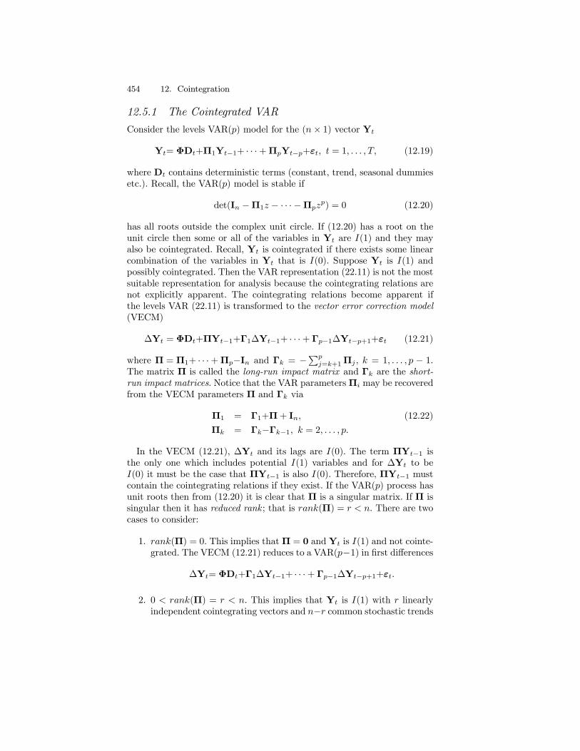
12.5.1 The Cointegrated VAR
Consider the levels VAR(p) model for the (n× 1) vector Yt
Yt= ΦDt+Π1Yt−1+ · · ·+ΠpYt−p+εt, t = 1, . . . , T, (12.19)
where Dt contains deterministic terms (constant, trend, seasonal dummiesetc.). Recall, the VAR(p) model is stable if
det(In −Π1z − · · ·−Πpzp) = 0 (12.20)
has all roots outside the complex unit circle. If (12.20) has a root on theunit circle then some or all of the variables in Yt are I(1) and they mayalso be cointegrated. Recall, Yt is cointegrated if there exists some linearcombination of the variables in Yt that is I(0). Suppose Yt is I(1) andpossibly cointegrated. Then the VAR representation (22.11) is not the mostsuitable representation for analysis because the cointegrating relations arenot explicitly apparent. The cointegrating relations become apparent ifthe levels VAR (22.11) is transformed to the vector error correction model(VECM)
∆Yt = ΦDt+ΠYt−1+Γ1∆Yt−1+ · · ·+ Γp−1∆Yt−p+1+εt (12.21)
where Π = Π1+ · · ·+Πp−In and Γk = −Pp
j=k+1Πj , k = 1, . . . , p − 1.The matrix Π is called the long-run impact matrix and Γk are the short-run impact matrices. Notice that the VAR parametersΠi may be recoveredfrom the VECM parameters Π and Γk via
Π1 = Γ1+Π+ In, (12.22)
Πk = Γk−Γk−1, k = 2, . . . , p.
In the VECM (12.21), ∆Yt and its lags are I(0). The term ΠYt−1 isthe only one which includes potential I(1) variables and for ∆Yt to beI(0) it must be the case that ΠYt−1 is also I(0). Therefore, ΠYt−1 mustcontain the cointegrating relations if they exist. If the VAR(p) process hasunit roots then from (12.20) it is clear that Π is a singular matrix. If Π issingular then it has reduced rank ; that is rank(Π) = r < n. There are twocases to consider:
1. rank(Π) = 0. This implies thatΠ = 0 and Yt is I(1) and not cointe-grated. The VECM (12.21) reduces to a VAR(p−1) in first differences
∆Yt= ΦDt+Γ1∆Yt−1+ · · ·+ Γp−1∆Yt−p+1+εt.
2. 0 < rank(Π) = r < n. This implies that Yt is I(1) with r linearlyindependent cointegrating vectors and n−r common stochastic trends

12.5 VAR Models and Cointegration 455
(unit roots)4. Since Π has rank r it can be written as the product
Π(n×n)
= α(n×r)
β(r×n)
0
where α and β are (n × r) matrices with rank(α) = rank(β) = r.The rows of β0 form a basis for the r cointegrating vectors and theelements of α distribute the impact of the cointegrating vectors tothe evolution of ∆Yt. The VECM (12.21) becomes
∆Yt= ΦDt+αβ0Yt−1+Γ1∆Yt−1+ · · ·+ Γp−1∆Yt−p+1+εt,
(12.23)where β0Yt−1 ∼ I(0) since β0 is a matrix of cointegrating vectors.
It is important to recognize that the factorizationΠ = αβ0 is not uniquesince for any r × r nonsingular matrix H we have
αβ0= αHH−1β0= (aH)(βH−10)0= a∗β∗0.
Hence the factorization Π = αβ0 only identifies the space spanned by thecointegrating relations. To obtain unique values of α and β0 requires furtherrestrictions on the model.
Example 80 A bivariate cointegrated VAR(1) model
Consider the bivariate VAR(1) model for Yt = (y1t, y2t)0
Yt= Π1Yt−1+²t.
The VECM is∆Yt= ΠYt−1+εt
where Π = Π1−I2. Assuming Yt is cointegrated there exists a 2 × 1 vec-tor β = (β1, β2)
0 such that β0Yt = β1y1t + β2y2t is I(0). Using thenormalization β1 = 1 and β2 = −β the cointegrating relation becomesβ0Yt = y1t − βy2t. This normalization suggests the stochastic long-runequilibrium relation
y1t = βy2t + ut
where ut is I(0) and represents the stochastic deviations from the long-runequilibrium y1t = βy2t.Since Yt is cointegrated with one cointegrating vector, rank(Π) = 1 and
can be decomposed as
Π = αβ0 =µ
α1α2
¶¡1 −β ¢
=
µα1 −α1βα2 −α2β
¶.
4To see thatYt has n−r common stochastic trends we have to look at the Beveridge-Nelson decomposition of the moving average representation of ∆Yt.
456 12. Cointegration
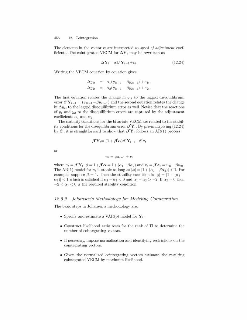
The elements in the vector α are interpreted as speed of adjustment coef-ficients. The cointegrated VECM for ∆Yt may be rewritten as
∆Yt= αβ0Yt−1+εt. (12.24)
Writing the VECM equation by equation gives
∆y1t = α1(y1t−1 − βy2t−1) + ε1t,
∆y2t = α2(y1t−1 − βy2t−1) + ε2t.
The first equation relates the change in y1t to the lagged disequilibriumerror β0Yt−1 = (y1t−1−βy2t−1) and the second equation relates the changein ∆y2t to the lagged disequilibrium error as well. Notice that the reactionsof y1 and y2 to the disequilibrium errors are captured by the adjustmentcoefficients α1 and α2.The stability conditions for the bivariate VECM are related to the stabil-
ity conditions for the disequilibrium error β0Yt. By pre-multiplying (12.24)by β0, it is straightforward to show that β0Yt follows an AR(1) process
β0Yt= (1+ β0α)β
0Yt−1+β0εt
or
ut = φut−1 + vt
where ut = β0Yt, φ = 1+β0α = 1+(α1−βα2) and vt = β0εt = u1t−βu2t.
The AR(1) model for ut is stable as long as |φ| = |1+ (α1−βα2)| < 1. Forexample, suppose β = 1. Then the stability condition is |φ| = |1 + (α1 −α2)| < 1 which is satisfied if α1−α2 < 0 and α1−α2 > −2. If α2 = 0 then−2 < α1 < 0 is the required stability condition.
12.5.2 Johansen’s Methodology for Modeling Cointegration
The basic steps in Johansen’s methodology are:
• Specify and estimate a VAR(p) model for Yt.
• Construct likelihood ratio tests for the rank of Π to determine thenumber of cointegrating vectors.
• If necessary, impose normalization and identifying restrictions on thecointegrating vectors.
• Given the normalized cointegrating vectors estimate the resultingcointegrated VECM by maximum likelihood.

12.5 VAR Models and Cointegration 457
12.5.3 Specification of Deterministic Terms
Following Johansen (1995), the deterministic terms in (12.23) are restrictedto the form
ΦDt = µt= µ0+µ1t
If the deterministic terms are unrestricted then the time series in Yt mayexhibit quadratic trends and there may be a linear trend term in the coin-tegrating relationships. Restricted versions of the trend parameters µ0 andµ1 limit the trending nature of the series in Yt. The trend behavior of Yt
can be classified into five cases:
1. Model H2(r): µt = 0 (no constant). The restricted VECM is
∆Yt= αβ0Yt−1+Γ1∆Yt−1+ · · ·+ Γp−1∆Yt−p+1+εt,
and all the series in Yt are I(1) without drift and the cointegratingrelations β0Yt have mean zero.
2. Model H∗1 (r): µt = µ0 = αρ0 (restricted constant). The restrictedVECM is
∆Yt= α(β0Yt−1 + ρ0)+Γ1∆Yt−1+ · · ·+ Γp−1∆Yt−p+1+εt,
the series in Yt are I(1) without drift and the cointegrating relationsβ0Yt have non-zero means ρ0.
3. Model H1(r): µt= µ0 (unrestricted constant). The restricted VECMis
∆Yt=µ0 +αβ0Yt−1+Γ1∆Yt−1+ · · ·+ Γp−1∆Yt−p+1+εt
the series in Yt are I(1) with drift vector µ0 and the cointegratingrelations β0Yt may have a non-zero mean.
4. ModelH∗(r): µt= µ0+αρ1t (restricted trend). The restricted VECMis
∆Yt = µ0 +α(β0Yt−1 + ρ1t)
+Γ1∆Yt−1+ · · ·+ Γp−1∆Yt−p+1+εt
the series in Yt are I(1) with drift vector µ0 and the cointegratingrelations β0Yt have a linear trend term ρ1t.
5. Model H(r): µt= µ0+µ1t (unrestricted constant and trend). The un-restricted VECM is
∆Yt= µ0 + µ1t+αβ0Yt−1+Γ1∆Yt−1+ · · ·+ Γp−1∆Yt−p+1+εt,
the series inYt are I(1) with a linear trend (quadratic trend in levels)and the cointegrating relations β0Yt have a linear trend.

458 12. Cointegration
Case 1: No constant
0 50 100 150 200
-22
46
8
Case 2: Restricted constant
0 50 100 150 200
05
1015
Case 3: Unrestricted constant
0 50 100 150 200
4080
120
Case 4: Restricted trend
0 50 100 150 200
4080
120
160
Case 5: Unrestricted trend
0 50 100 150 200
500
1500
3000
FIGURE 12.6. Simulated Yt from bivariate cointegrated VECM for five trendcases.
Case 1: No constant
0 50 100 150 200
-20
24
Case 2: Restricted constant
0 50 100 150 200
68
1012
Case 3: Unrestricted constant
0 50 100 150 200
46
810
Case 4: Restricted trend
0 50 100 150 200
1520
2530
Case 5: Unrestricted trend
0 50 100 150 200
-20
-10
0
FIGURE 12.7. Simulated β0Yt from bivariate cointegrated VECM for five trendcases.

12.5 VAR Models and Cointegration 459
Simulated data from the five trend cases for a bivariate cointegratedVAR(1) model are illustrated in Figures 12.6 and 12.7. Case I is not reallyrelevant for empirical work. The restricted contstant Case II is appropriatefor non-trending I(1) data like interest rates and exchange rates. The un-restriced constant Case III is appropriate for trending I(1) data like assetprices, macroeconomic aggregates (real GDP, consumption, employmentetc). The restricted trend case IV is also appropriate for trending I(1) asin Case III. However, notice the deterministic trend in the cointegratingresidual in Case IV as opposed to the stationary residual in case III. Fi-nally, the unrestricted trend Case V is appropriate for I(1) data with aquadratic trend. An example might be nominal price data during times ofextreme inflation.
12.5.4 Likelihood Ratio Tests for the Number of CointegratingVectors
The unrestricted cointegrated VECM (12.23) is denoted H(r). The I(1)model H(r) can be formulated as the condition that the rank of Π is lessthan or equal to r. This creates a nested set of models
H(0) ⊂ · · · ⊂ H(r) ⊂ · · · ⊂ H(n)
where H(0) represents the non-cointegrated VAR model with Π = 0 andH(n) represents an unrestricted stationary VAR(p) model. This nestedformulation is convenient for developing a sequential procedure to test forthe number r of cointegrating relationships.Since the rank of the long-run impact matrixΠ gives the number of coin-
tegrating relationships in Yt, Johansen formulates likelihood ratio (LR)statistics for the number of cointegrating relationships as LR statistics fordetermining the rank ofΠ. These tests are based on the estimated eigenval-ues λ1 > λ2 > · · · > λn of the matrixΠ
5. These eigenvalues also happen toequal the squared canonical correlations between ∆Yt and Yt−1 correctedfor lagged ∆Yt and Dt and so lie between 0 and 1. Recall, the rank of Πis equal to the number of non-zero eigenvalues of Π.
Johansen’s Trace Statistic
Johansen’s LR statistic tests the nested hypotheses
H0(r) : r = r0 vs. H1(r0) : r > r0
The LR statistic, called the trace statistic, is given by
LRtrace(r0) = −TnX
i=r0+1
ln(1− λi)
5The calculation of the eigenvalues λi (i = 1, . . . , n) is described in the appendix.

460 12. Cointegration
If rank(Π) = r0 then λr0+1, . . . , λn should all be close to zero and LRtrace(r0)
should be small. In contrast, if rank(Π) > r0 then some of λr0+1, . . . , λnwill be nonzero (but less than 1) and LRtrace(r0) should be large. Theasymptotic null distribution of LRtrace(r0) is not chi-square but insteadis a multivariate version of the Dickey-Fuller unit root distribution whichdepends on the dimension n − r0 and the specification of the determinis-tic terms. Critical values for this distribution are tabulated in Osterwald-Lenum (1992) for the five trend cases discussed in the previous section forn− r0 = 1, . . . , 10.
Sequential Procedure for Determining the Number of CointegratingVectors
Johansen proposes a sequential testing procedure that consistently deter-mines the number of cointegrating vectors. First test H0(r0 = 0) againstH1(r0 > 0). If this null is not rejected then it is concluded that there are nocointegrating vectors among the n variables in Yt. If H0(r0 = 0) is rejectedthen it is concluded that there is at least one cointegrating vector and pro-ceed to test H0(r0 = 1) against H1(r0 > 1). If this null is not rejected thenit is concluded that there is only one cointegrating vector. If the null is re-jected then it is concluded that there is at least two cointegrating vectors.The sequential procedure is continued until the null is not rejected.
Johansen’s Maximum Eigenvalue Statistic
Johansen also derives a LR statistic for the hypotheses
H0(r0) : r = r0 vs. H1(r0) : r0 = r0 + 1
The LR statistic, called the maximum eigenvalue statistic, is given by
LRmax(r0) = −T ln(1− λr0+1)
As with the trace statistic, the asymptotic null distribution of LRmax(r0)is not chi-square but instead is a complicated function of Brownian mo-tion, which depends on the dimension n − r0 and the specification of thedeterministic terms. Critical values for this distribution are tabulated inOsterwald-Lenum (1992) for the five trend cases discussed in the previoussection for n− r0 = 1, . . . , 10.
Finite Sample Correction to LR Tests
Reinsel and Ahn (1992) and Reimars (1992) have suggested that the LRtests perform better in finite samples if the factor T − np is used insteadof T in the construction of the LR tests.
12.5 VAR Models and Cointegration 461
12.5.5 Testing Hypothesis on Cointegrating Vectors Using theS+FinMetrics Function coint
This section describes how to test for the number of cointegrating vectors,and how to perform certain tests for linear restrictions on the long-run βcoefficients.
Testing for the Number of Cointegrating Vectors
The Johansen LR tests for determining the number of cointegrating vec-tors in multivariate time series may be computed using the S+FinMetricsfunction coint. The function coint has arguments
> args(coint)
function(Y, X = NULL, lags = 1, trend = "c", H = NULL,
b = NULL, save.VECM = T)
where Y is a matrix, data frame or “timeSeries” containing the I(1)variables in Yt, X is a numeric object representing exogenous variables tobe added to the VECM, lags denotes the number of lags in the VECM(one less than the number of lags in the VAR representation), trend deter-mines the trend case specification, and save.VECM determines if the VECMinformation is to be saved. The arguments H and b will be explained later.The result of coint is an object of class “coint” for which there are printand summary methods. The use of coint is illustrated with the followingexamples.
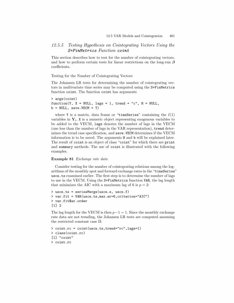
Example 81 Exchange rate data
Consider testing for the number of cointegrating relations among the log-arithms of the monthly spot and forward exchange rates in the “timeSeries”uscn.ts examined earlier. The first step is to determine the number of lagsto use in the VECM. Using the S+FinMetrics function VAR, the lag lengththat minimizes the AIC with a maximum lag of 6 is p = 2:
> uscn.ts = seriesMerge(uscn.s, uscn.f)
> var.fit = VAR(uscn.ts,max.ar=6,criterion="AIC")
> var.fit$ar.order
[1] 2
The lag length for the VECM is then p−1 = 1. Since the monthly exchangerate data are not trending, the Johansen LR tests are computed assumingthe restricted constant case II:
> coint.rc = coint(uscn.ts,trend="rc",lags=1)
> class(coint.rc)
[1] "coint"
> coint.rc

462 12. Cointegration
Call:
coint(Y = uscn.ts, lags = 1, trend = "rc")
Trend Specification:
H1*(r): Restricted constant
Trace tests significant at the 5% level are flagged by ’ +’.
Trace tests significant at the 1% level are flagged by ’++’.
Max Eigenvalue tests significant at the 5% level are flagged
by ’ *’.
Max Eigenvalue tests significant at the 1% level are flagged
by ’**’.
Tests for Cointegration Rank:
Eigenvalue Trace Stat 95% CV 99% CV Max Stat
H(0)++** 0.0970 32.4687 19.9600 24.6000 24.8012
H(1) 0.0311 7.6675 9.2400 12.9700 7.6675
95% CV 99% CV
H(0)++** 15.6700 20.2000
H(1) 9.2400 12.9700
Recall, the number of cointegrating vectors is equal to the number of non-zero eigenvalues ofΠ. The two estimated eigenvalues are 0.0970 and 0.0311.The first row in the table gives LRtrace(0) and LRmax(0) for testing the nullof r0 = 0 cointegrating vectors as well as the 95% and 99% quantiles of theappropriate asymptotic distributions taken from the tables in Osterwald-Lenum (1992). Both the trace and maximum eigenvalue statistics reject ther0 = 0 null at the 1% level. The second row in the table gives LRtrace(1)and LRmax(1) for testing the null of r0 = 1. Neither statistic rejects thenull that r0 = 1.The summary method gives the same output as print as well as the un-
normalized cointegrating vectors, adjustment coefficients and the estimateof Π.
Testing Linear Restrictions on Cointegrating Vectors
The coint function can also be used to test linear restrictions on the coin-tegrating vectors β. Two types of restrictions are currently supported: thesame linear restrictions on all cointegrating vectors in β; some cointegratingvectors in β are assumed known. Following Johansen (1995), two examplesare given illustrating how to use the coint function to test linear restric-tions on β.
Example 82 Johansen’s Danish data

12.5 VAR Models and Cointegration 463
The "timeSeries" data set johansen.danish in S+FinMetrics containsthe monthly Danish data used in Johansen (1995), with the columns LRM,LRY, LPY, IBO, IBE representing the log real money supply (mt), log realincome (yt), log prices, bond rate (i
bt) and deposit rate (i
dt ), respectively.
Johansen (1995) considered testing the cointegrating relationship amongmt, yt, i
bt and idt . A natural hypothesis is that the velocity of money is a
function of the interest rates, or the cointegrating relation contains mt andyt only through the term mt − yt. For R
0 = (1, 1, 0, 0), this hypothesis canbe represented as a linear restriction on β:
H0 : R0β = 0 or β =HΨ (12.25)
where Ψ are the unknown parameters in the cointegrating vectors β, H =R⊥ and R⊥ is the orthogonal complement of R such that R0R⊥ = 0.Johansen (1995) showed that the null hypothesis (12.25) against the alter-native of unrestricted r cointegrating relations H(r) can be tested using alikelihood ratio statistic, which is asymptotically distributed as a χ2 withr(n− s) degree of freedom where s is the number of columns in H.To test the hypothesis that the coefficients of mt and yt add up to zero
in the cointegrating relations, Johansen (1995) considered a restricted con-stant model. In this case, R0 = (1, 1, 0, 0, 0) since the restricted constantalso enters the cointegrating space. Given the restriction matrix R, thematrix H can be computed using the perpMat function in S+FinMetrics:
> R = c(1, 1, 0, 0, 0)
> H = perpMat(R)
> H
[,1] [,2] [,3] [,4]
[1,] -1 0 0 0
[2,] 1 0 0 0
[3,] 0 1 0 0
[4,] 0 0 1 0
[5,] 0 0 0 1
Now the test can be simply performed by passing the matrix H to thecoint function:
> restr.mod1 = coint(johansen.danish[,c(1,2,4,5)],
+ trend="rc", H=H)
The result of the test can be shown by calling the generic print methodon restr.mod1 with the optional argument restrictions=T:
> print(restr.mod1, restrictions=T)
Call:
coint(Y = johansen.danish[, c(1, 2, 4, 5)], trend = "rc",
H = H)

464 12. Cointegration
Trend Specification:
H1*(r): Restricted constant
Tests for Linear Restriction on Coint Vectors:
Null hypothesis: the restriction is true
Stat Dist df P-value
H(1) 0.0346 chi-square 1 0.8523
H(2) 0.2607 chi-square 2 0.8778
H(3) 4.6000 chi-square 3 0.2035
H(4) 6.0500 chi-square 4 0.1954
For unrestricted sequential cointegration testing, the statistics in the out-put are labeled according to the null hypothesis, such as H(0), H(1), etc.However, when restrictions are imposed, the statistics in the output printedwith restrictions=T are labeled according to the alternative hypothesis,such as H(1), H(2), etc. In the above output, the null hypothesis can-not be rejected against the alternatives of H(1), H(2), H(3) and H(4) atconventional levels of significance.After confirming that the cointegrating coefficients on mt and yt add
up to zero, it is interesting to see if (1,−1, 0, 0, 0) actually is a cointegrat-ing vector. In general, to test the null hypothesis that some cointegratingvectors in β are equal to b:
H0 : β = (b,Ψ)
where b is the n × s matrix of known cointegrating vectors and Ψ is then×(r−s) matrix of unknown cointegrating vectors, Johansen (1995) showedthat a likelihood ratio statistic can be used, which is asymptotically dis-tributed as a χ2 with s(n− r) degrees of freedom. This test can be simplyperformed by setting the optional argument b to the known cointegratingvectors. For example,
> b = as.matrix(c(1,-1,0,0,0))
> restr.mod2 = coint(johansen.danish[,c(1,2,4,5)],
+ trend="rc", b=b)
> print(restr.mod2, restrictions=T)
Trend Specification:
H1*(r): Restricted constant
Tests for Known Coint Vectors:
Null hypothesis: the restriction is true
Stat Dist df P-value
H(1) 29.7167 chi-square 4 0.0000
H(2) 8.3615 chi-square 3 0.0391
12.5 VAR Models and Cointegration 465
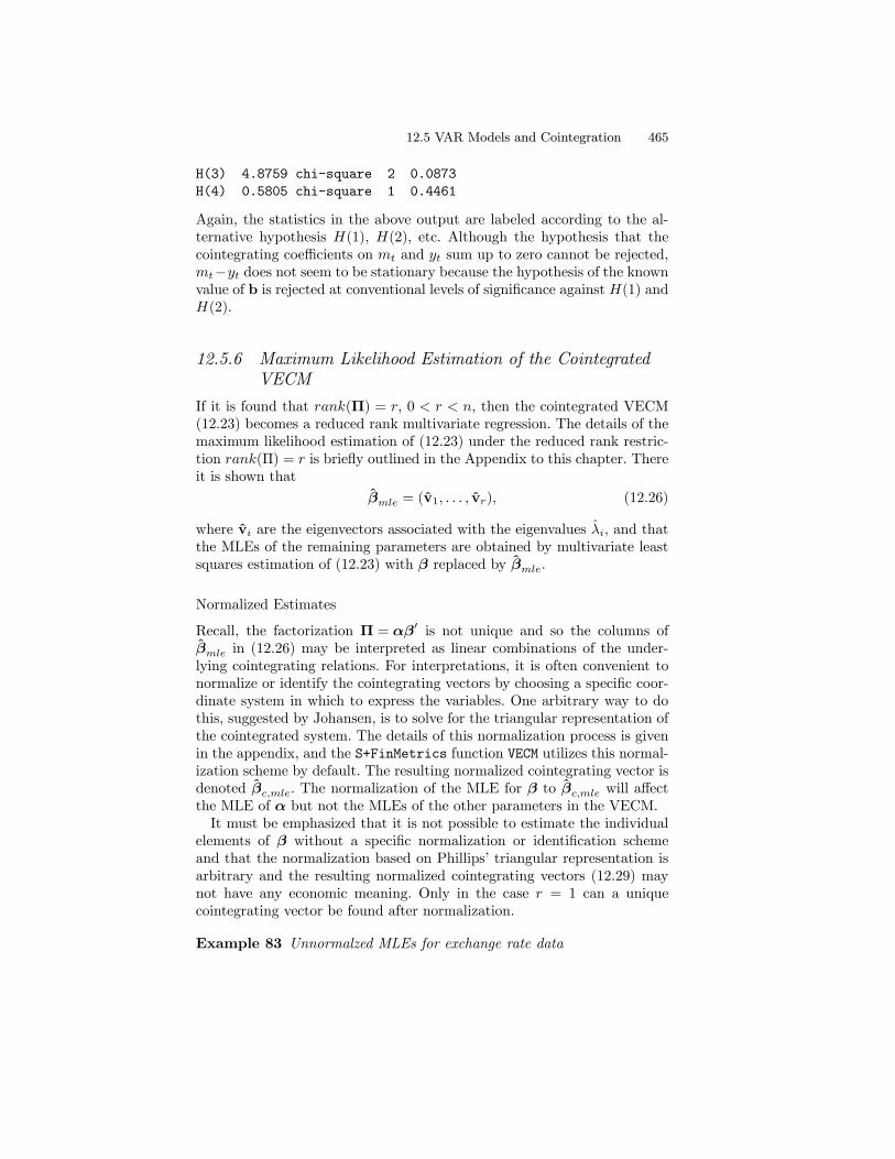
H(3) 4.8759 chi-square 2 0.0873
H(4) 0.5805 chi-square 1 0.4461
Again, the statistics in the above output are labeled according to the al-ternative hypothesis H(1), H(2), etc. Although the hypothesis that thecointegrating coefficients on mt and yt sum up to zero cannot be rejected,mt−yt does not seem to be stationary because the hypothesis of the knownvalue of b is rejected at conventional levels of significance against H(1) andH(2).
12.5.6 Maximum Likelihood Estimation of the CointegratedVECM
If it is found that rank(Π) = r, 0 < r < n, then the cointegrated VECM(12.23) becomes a reduced rank multivariate regression. The details of themaximum likelihood estimation of (12.23) under the reduced rank restric-tion rank(Π) = r is briefly outlined in the Appendix to this chapter. Thereit is shown that
βmle = (v1, . . . , vr), (12.26)
where vi are the eigenvectors associated with the eigenvalues λi, and thatthe MLEs of the remaining parameters are obtained by multivariate leastsquares estimation of (12.23) with β replaced by βmle.
Normalized Estimates
Recall, the factorization Π = αβ0 is not unique and so the columns ofβmle in (12.26) may be interpreted as linear combinations of the under-lying cointegrating relations. For interpretations, it is often convenient tonormalize or identify the cointegrating vectors by choosing a specific coor-dinate system in which to express the variables. One arbitrary way to dothis, suggested by Johansen, is to solve for the triangular representation ofthe cointegrated system. The details of this normalization process is givenin the appendix, and the S+FinMetrics function VECM utilizes this normal-ization scheme by default. The resulting normalized cointegrating vector isdenoted βc,mle. The normalization of the MLE for β to βc,mle will affectthe MLE of α but not the MLEs of the other parameters in the VECM.It must be emphasized that it is not possible to estimate the individual
elements of β without a specific normalization or identification schemeand that the normalization based on Phillips’ triangular representation isarbitrary and the resulting normalized cointegrating vectors (12.29) maynot have any economic meaning. Only in the case r = 1 can a uniquecointegrating vector be found after normalization.
Example 83 Unnormalzed MLEs for exchange rate data

466 12. Cointegration
The unnormalized cointegrating vector assuming r0 = 1 may also beextracted directly from the “coint” object:
> coint.rc$coint.vectors[1,]
USCNS USCNF Intercept*
-739.0541 743.314 2.023532
Notice in the case of a restricted constant, the last coefficient in βmle is anestimate of the restricted constant. Normalizing on USCNS by dividing eachelement in βmle by −739.0541 gives> coint.rc$coint.vectors[1,]/
+ as.numeric(-coint.rc$coint.vectors[1,1])
USCNS USCNF Intercept*
-1 1.005764 0.002738003
The normalized MLEs, βc,mle = (−1, 1.006)0 and µc = 0.0027 are almost
identical to the least squares estimates β = (1,−1.004)0 and µ = 0.0023found earlier.
Asymptotic Distributions
Let βc,mle denote the MLE of the normalized cointegrating matrix βc.
Johansen (1995) shows that T (vec(βc,mle) − vec(βc)) is asymptotically(mixed) normally distributed and that a consistent estimate of the asymp-totic covariance of βc,mle is given by
[avar(vec(βc,mle)) =
T−1(In−βc,mlec0)S−111 (In−βc,mlec
0)0 ⊗³α0c,mleΩ
−1αc,mle
´−1(12.27)
Notice that this result implies that βc,mlep→ βc at rate T instead of the
usual rate T 1/2. Hence, like the least squares estimator, βc,mle is super con-sistent. However, unlike the least squares estimator, asymptotically validstandard errors may be compute using the square root of the diagonalelements of (12.27).
12.5.7 Maximum Likelihood Estimation of the CointegratedVECM Using the S+FinMetrics Function VECM
Once the number of cointegrating vectors is determined from the cointfunction, the maximum likelihood estimates of the full VECM may beobtained using the S+FinMetrics function VECM. The arguments expectedby VECM are
> args(VECM)
function(object, coint.rank = 1, coint.vec = NULL, X = NULL,
unbiased = T, lags = 1, trend = "c", levels = F)

12.5 VAR Models and Cointegration 467
where object is either a “coint” object, usually produced by a call to thefunction coint, or a rectangular data object. If object is a “coint” objectthen coint.rank specifies the rank of Π to determine the number of coin-tegrating vectors to be used in the fitted VECM. The cointegrating vectorsare then normalized using the Phillips’ triangular representation describedin the appendix. The lag length and trend specification for the VECM isobtained from the information in the “coint” object. The lag length inthe fitted VECM, however, is one less than the lag length specified in the“coint” object. If object is a rectangular data object, then coint.vecmust be assigned a matrix whose columns represent pre-specified cointe-grating vectors. The argument lags is then used to specify the lag length ofthe VECM, and trend is used to set the trend specification. The optionalargument X is used to specify any exogenous variables (e.g. dummy variablesfor events) other than a constant or trend. The optional argument levelsdetermines if the VECM is to be fit to the levels Yt or to the first differ-ences ∆Yt, and determines if forecasts are to be computed for the levels orthe first differences. The result of VECM is an object of class “VECM”, whichinherits from “VAR” for which there are print, summary, plot, cpredictand predict methods and extractor functions coef, fitted, residualsand vcov. Since “VECM” objects inherit from “VAR” objects, most of themethod and extractor functions for “VECM” objects work similarly to thosefor “VAR” objects. The use of VECM is illustrated with the following exam-ples.
Example 84 Maximum likelihood estimation of the VECM for exchangerate data
Using the “coint” object coint.rc computed from the VAR(2) modelwith a restricted constant, the VECM(1) with a restricted constant for theexchange rate data is computed using
> vecm.fit = VECM(coint.rc)
> class(vecm.fit)
[1] "VECM"
> inherits(vecm.fit,"VAR")
[1] T
The print method gives the basic output
> vecm.fit
Call:
VECM(test = coint.rc)
Cointegrating Vectors:
coint.1
USCNS 1.0000

468 12. Cointegration
USCNF -1.0058
Intercept* -0.0027
VECM Coefficients:
USCNS USCNF
coint.1 1.7771 1.9610
USCNS.lag1 1.1696 1.2627
USCNF.lag1 -1.2832 -1.3679
Std. Errors of Residuals:
USCNS USCNF
0.0135 0.0136
Information Criteria:
logL AIC BIC HQ
2060.2 -4114.4 -4103.9 -4110.1
total residual
Degree of freedom: 243 240
Time period: from Apr 1976 to Jun 1996
The print method output is similar to that created by the VAR function.The output labeled Cointegrating Vectors: gives the estimated cointe-grating vector coefficients normalized on the first variable in the specifica-tion of the VECM. To see standard errors for the estimated coefficients usethe summary method
> summary(vecm.fit)
Call:
VECM(test = coint.rc)
Cointegrating Vectors:
coint.1
1.0000
USCNF -1.0058
(std.err) 0.0031
(t.stat) -326.6389
Intercept* -0.0027
(std.err) 0.0007
(t.stat) -3.9758
VECM Coefficients:

12.5 VAR Models and Cointegration 469
USCNS USCNF
coint.1 1.7771 1.9610
(std.err) 0.6448 0.6464
(t.stat) 2.7561 3.0335
USCNS.lag1 1.1696 1.2627
(std.err) 0.9812 0.9836
(t.stat) 1.1921 1.2837
USCNF.lag1 -1.2832 -1.3679
(std.err) 0.9725 0.9749
(t.stat) -1.3194 -1.4030
Regression Diagnostics:
USCNS USCNF
R-squared 0.0617 0.0689
Adj. R-squared 0.0538 0.0612
Resid. Scale 0.0135 0.0136
Information Criteria:
logL AIC BIC HQ
2060.2 -4114.4 -4103.9 -4110.1
total residual
Degree of freedom: 243 240
Time period: from Apr 1976 to Jun 1996
The VECM fit may be inspected graphically using the generic plotmethod
> plot(vecm.fit)
Make a plot selection (or 0 to exit):
1: plot: All
2: plot: Response and Fitted Values
3: plot: Residuals
4: plot: Normal QQplot of Residuals
5: plot: ACF of Residuals
6: plot: PACF of Residuals
7: plot: ACF of Squared Residuals
8: plot: PACF of Squared Residuals
9: plot: Cointegrating Residuals
10: plot: ACF of Cointegrating Residuals
11: plot: PACF of Cointegrating Residuals
12: plot: ACF of Squared Cointegrating Residuals

470 12. Cointegration
-0.0
06-0
.002
0.00
2
1977 1979 1981 1983 1985 1987 1989 1991 1993 1995
coint.1
Cointegrating Residuals
FIGURE 12.8. Cointegrating residual from maximum likelihood estimation ofVECM(1) for exchange rate data.
13: plot: PACF of Squared Cointegrating Residuals
Selection:
The first eight plot options are the same as those created for a "VAR" object.The remaining plot options allow a graphical inspection of the cointegrat-ing residual. For example, plot option 9 is illustrated in Figure 12.8. Theestimated cointegrating residual appears to be I(0).
Example 85 Estimate VECM with pre-specified cointegrating vector
For the exchange rate data, the MLE of the normalized cointegratingvector is close to (1,−1)0, and the estimate of the restricted constant isclose to zero. These are the values implied by the FRUH. To estimate aVECM(1) imposing β = (1,−1)0 and µt = 0 use
> beta.true = as.matrix(c(1,-1, 0))
> dimnames(beta.true) = list(c("USCNS","USCNF","Intercept"),
+ "coint.1")
> vecm.fruh.fit = VECM(uscn.ts, coint.vec = beta.true,
+ lags = 1, trend = "rc")
Since the restricted constant lies in the cointegrating space, the last ele-ment of the pre-specified cointegrating vector is the value of the restrictedconstant. A summary of the restricted VECM fit is:
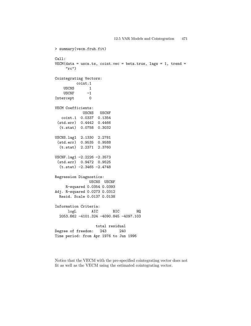
12.5 VAR Models and Cointegration 471
> summary(vecm.fruh.fit)
Call:
VECM(data = uscn.ts, coint.vec = beta.true, lags = 1, trend =
"rc")
Cointegrating Vectors:
coint.1
USCNS 1
USCNF -1
Intercept 0
VECM Coefficients:
USCNS USCNF
coint.1 0.0337 0.1354
(std.err) 0.4442 0.4466
(t.stat) 0.0758 0.3032
USCNS.lag1 2.1330 2.2781
(std.err) 0.9535 0.9588
(t.stat) 2.2371 2.3760
USCNF.lag1 -2.2226 -2.3573
(std.err) 0.9472 0.9525
(t.stat) -2.3465 -2.4748
Regression Diagnostics:
USCNS USCNF
R-squared 0.0354 0.0393
Adj. R-squared 0.0273 0.0312
Resid. Scale 0.0137 0.0138
Information Criteria:
logL AIC BIC HQ
2053.662 -4101.324 -4090.845 -4097.103
total residual
Degree of freedom: 243 240
Time period: from Apr 1976 to Jun 1996
Notice that the VECM with the pre-specified cointegrating vector does notfit as well as the VECM using the estimated cointegrating vector.

472 12. Cointegration
12.5.8 Forecasting from the VECM
Forecasts from a VECM are computed by first transforming the VECM toa VAR using (12.22), and then using the forecasting algorithms for VARmodels described in the previous chapter. For VECM models, one mayforecast the changes in the variables, ∆Yt, or the levels of the variables Yt.The generic S+FinMetrics functions predict and cpredict are used tocompute unconditional and conditional forecasts from a “VECM” object. Thefollowing example illustrates the use of the predict method to computeforecasts for the differences and levels of the exchange rate data.
Example 86 Forecasts from VECM fit to exchange rate data
The “VECM” object vecm.fit was produced with the optional argumentlevels=F. Consequently, the predict method will produce forecasts forthe changes in st and ft. To compute h-step forecasts for ∆st and ∆ft forh = 1, . . . , 12 use
> vecm.fcst = predict(vecm.fit,n.predict=12)
> class(vecm.fcst)
[1] "forecast"
To see the forecast and forecast standard errors use
> summary(vecm.fcst)
Predicted Values with Standard Errors:
USCNS USCNF
1-step-ahead -0.0105 -0.0110
(std.err) 0.0136 0.0136
2-step-ahead -0.0130 -0.0139
(std.err) 0.0183 0.0183
...
12-step-ahead -0.0237 -0.0260
(std.err) 0.0435 0.0432
By default, the forecasts are computed using the chain-rule of forecasting.To compute simulation-based forecasts use method = "mc" or method ="bootstrap" in the call to predict.To see the forecasts with standard error bands along the original data
use
> plot(vecm.fcst, xold=diff(uscn.ts), n.old=12)
Since the forecasts are of the first differenced data, the data passed to xoldmust be first differenced. The resulting plot is shown in Figure 12.9.To compute forecasts for the levels st and ft, re-fit the VECM with the
optional argument levels=T

12.5 Appendix: MLE of a Cointegrated VECM 473
-0.0
6-0
.04
-0.0
20.
00.
02
235 240 245 250 255
USCNF
-0.0
6-0
.04
-0.0
20.
00.
02
235 240 245 250 255
USCNS
index
valu
es
FIGURE 12.9. VECM forecasts of first differences of exchange rate data.
> vecm.fit.level = VECM(coint.rc, levels=T)
and then call the predict method as before
> vecm.fcst.level = predict(vecm.fit.level, n.predict=12)
> summary(vecm.fcst.level)
Predicted Values with Standard Errors:
USCNS USCNF
1-step-ahead -0.3150 -0.3154
(std.err) 0.0136 0.0136
2-step-ahead -0.3157 -0.3161
(std.err) 0.0183 0.0183
...
12-step-ahead -0.3185 -0.3193
(std.err) 0.0435 0.0432
To plot the forecasts use
> plot(vecm.fcst.level, xold=uscn.ts, n.old=12)
The resulting plot is shown in Figure 12.10.

474 12. Cointegration
-0.3
6-0
.34
-0.3
2-0
.30
-0.2
8
235 240 245 250 255
USCNF
-0.3
6-0
.34
-0.3
2-0
.30
-0.2
8
235 240 245 250 255
USCNS
index
valu
es
FIGURE 12.10. VECM forecasts of levels of exchange rate data.
12.6 Appendix: Maximum Likelihood Estimationof a Cointegrated VECM
The following brief discussion of maximum likelihood estimation of thecointegrated VECM (12.23) follows Hamilton (1994) and Johansen (1995).For simplicity, assume the absence of deterministic terms.
• Concentrate the likelihood function with respect to the error covari-ance matrix and short-run dynamics by estimating the regressions
∆Yt = Γ1∆Yt−1+ · · · Γp−1∆Yt−p+1+Ut
Yt = Φ1∆Yt−1+ · · · Φp−1∆Yt−p+1+Vt
• Form the sample covariance matrices
S00 =1
T
TXt=1
UtU0t, S01 =
1
T
TXt=1
UtV0t, S11 =
1
T
TXt=1
VtV0t
• Solve the eigenvalue problem
|λS11 − S10S−100 S01| = 0

12.6 Appendix: Maximum Likelihood Estimation of aCointegrated VECM 475
giving ordered eigenvalues6 λ1 > λ2 > · · · > λn and associated eigen-vectors v1, v2, . . . , vn that satisfy
λiS11vi = S10S−100 S01, i = 1, . . . , n
VS11V = In
where V = [v1, . . . , vn]
• The unnormalized MLE for the (n× r) matrix β based on 0 < r < ncointegrating vectors is given by the first r eigenvectors
βmle = (v1, . . . , vr)
• Form the normalized estimator βc,mle by imposing the appropriatenormalizing and identifying restrictions. The MLE for the normalizedestimator of α may be computed as
αc,mle = S01βc,mle
• The maximum likelihood estimators for the remaining parametersmay be obtained by multivariate least squares of the VECM with βreplaced by βc,mle
∆Yt= αcβ0c,mleYt−1+Γ1∆Yt−1+ · · ·+ Γp−1∆Yt−p+1+εt
• The maximized value of the likelihood function based on r cointe-grating vectors used in the construction of LR tests for the numberof cointegrating vectors is
L−2/Tmax ∝ |S00|rY
i=1
(1− λi)
• Estimates of the orthogonal complements of αc and βc are given by
αc,⊥ = S−100 S11(vr+1, . . . , vn)
βc,⊥ = S11(vr+1, . . . , vn)
Let c be any (n× r) matrix such that β0c has full rank. Then β may benormalized as
βc = β(c0β)−1
6These eigenvalues are the squared canonical correlations between Yt and ∆Yt cor-rected for ∆Yt−1, . . . ,∆Yt−p+1. Johansen (1995) describes how to solve for the eigen-values.
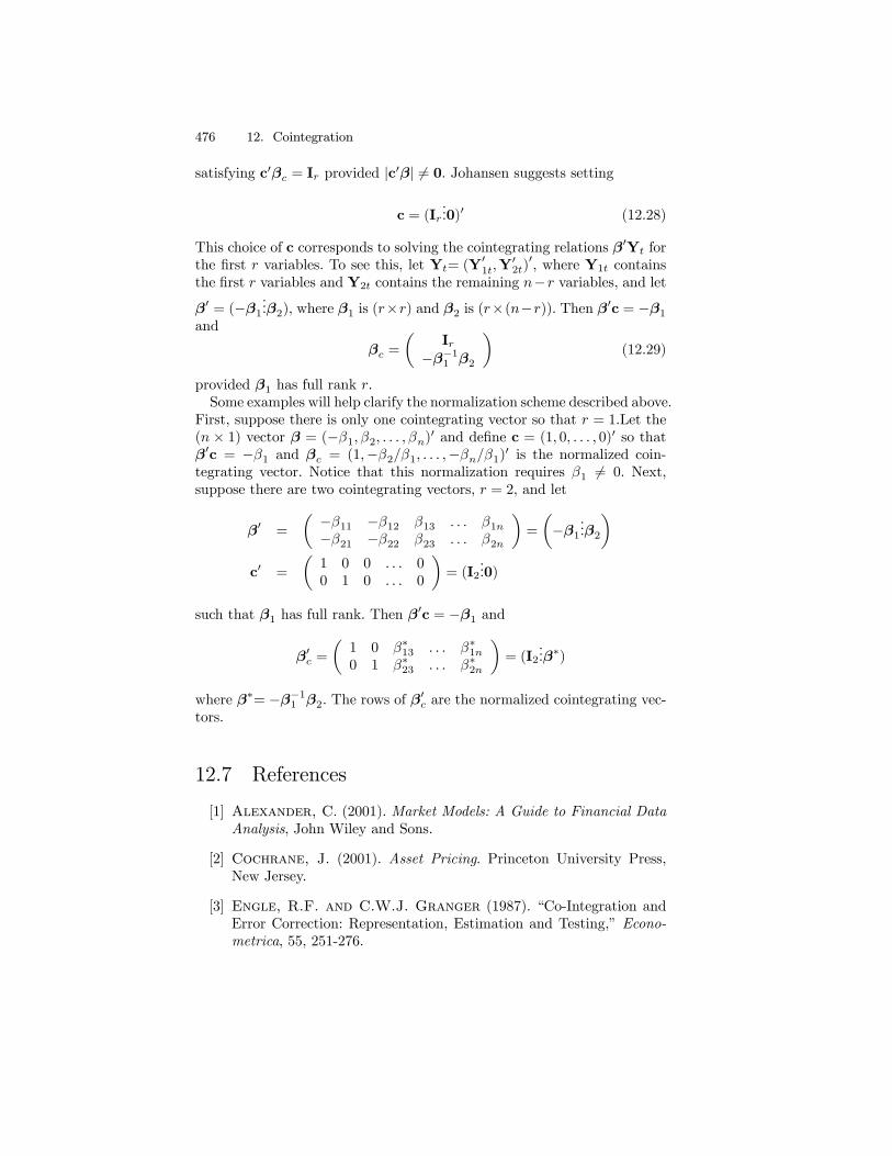
476 12. Cointegration
satisfying c0βc = Ir provided |c0β| 6= 0. Johansen suggests setting
c = (Ir...0)0 (12.28)
This choice of c corresponds to solving the cointegrating relations β0Yt forthe first r variables. To see this, let Yt= (Y
01t,Y
02t)
0, where Y1t containsthe first r variables and Y2t contains the remaining n−r variables, and letβ0 = (−β1
...β2), where β1 is (r×r) and β2 is (r×(n−r)). Then β0c = −β1and
βc =
µIr
−β−11 β2
¶(12.29)
provided β1 has full rank r.Some examples will help clarify the normalization scheme described above.
First, suppose there is only one cointegrating vector so that r = 1.Let the(n × 1) vector β = (−β1, β2, . . . , βn)0 and define c = (1, 0, . . . , 0)0 so thatβ0c = −β1 and βc = (1,−β2/β1, . . . ,−βn/β1)0 is the normalized coin-tegrating vector. Notice that this normalization requires β1 6= 0. Next,suppose there are two cointegrating vectors, r = 2, and let
β0 =
µ −β11 −β12 β13 . . . β1n−β21 −β22 β23 . . . β2n
¶=
µ−β1
...β2
¶c0 =
µ1 0 0 . . . 00 1 0 . . . 0
¶= (I2
...0)
such that β1 has full rank. Then β0c = −β1 and
β0c =µ1 0 β∗13 . . . β∗1n0 1 β∗23 . . . β∗2n
¶= (I2
...β∗)
where β∗= −β−11 β2. The rows of β0c are the normalized cointegrating vec-
tors.
12.7 References
[1] Alexander, C. (2001). Market Models: A Guide to Financial DataAnalysis, John Wiley and Sons.
[2] Cochrane, J. (2001). Asset Pricing. Princeton University Press,New Jersey.
[3] Engle, R.F. and C.W.J. Granger (1987). “Co-Integration andError Correction: Representation, Estimation and Testing,” Econo-metrica, 55, 251-276.

12.7 References 477
[4] Granger, C.W.J. and P.E. Newbold (1974). “Spurious Regres-sion in Econometrics,” Journal of Econometrics, 2, 111-120.
[5] Hamilton, J.D. (1994). Time Series Analysis, Princeton UnversityPress, New Jersey.
[6] Hansen, B.E. (1992). “Efficient Estimation and Testing of Cointe-grating Vectors in the Presence of Deterministic Trends,” Journal ofEconometrics, 53, 87-121.
[7] Hayashi, F. (2000). Econometrics, Princeton University Press, NewJersey.
[8] Johansen, S. (1988). “Statistical Analysis of Cointegration Vec-tors,” Journal of Economic Dynamics and Control, 12, 231-254.
[9] Johansen, S. (1995). Likelihood Based Inference in CointegratedVector Error Correction Models, Oxford University Press, Oxford.
[10] MacKinnon, J. (1996). “Numerical Distribution Functions for UnitRoot and Cointegration Tests,” Journal of Applied Econometrics, 11,601-618.
[11] Mills, T. (1999). The Econometric Analysis of Financial Time Se-ries, Cambridge University Press, Cambridge.
[12] Osterwald-Lenum, M. (1992). “A Note with Quantiles of the Asymp-totic Distribution of the Maximum Likelihood Cointegration RankStatistics,” Oxford Bulletin of Economics and Statistics,54, 461-472.
[13] Phillips, P.C.B. (1986). “Understanding Spurious Regression inEconometrics,” Journal of Econometrics, 33, 311-340.
[14] Phillips, P.C.B. (1991). “Optimal Inference in Cointegrated Sys-tems,” Econometrica, 59, 283-306.
[15] Phillips, P.C.B. and S. Ouliaris (1990). “Asymptotic Propertiesof Residual Based Tests for Cointegration,” Econometrica, 58, 73-93.
[16] Reimars, H.-E. (1992). “Comparisons of Tests for Multivariate Coin-tegration,” Statistical Papers, 33, 335-359.
[17] Reinsel, G.C. and S.K. Ahn (1992). “Vector Autoregression Mod-els with Unit Roots and Reduced Rank Structure: Estimation, Likeli-hood Ratio Test, and Forecasting,” Journal of Time Series Analysis,13, 353-375.
[18] Sims, C.A., J.H. Stock and M.W. Watson (1990). “Inference inLinear Time Series Models with Some Unit Roots,” Econometrica,58, 113-144.

478 12. Cointegration
[19] Stock, J.H. (1987). “Asymptotic Properties of Least Squares Esti-mation of Cointegrating Vectors,” Econometrica, 55, 1035-1056.
[20] Stock, J.H. and M.W. Watson (1989). “Variable Trends in Eco-nomic Time Series,” Journal of Economic Perspectives, Vol. 2(3),147-174.
[21] Stock, J.H. and M.W. Watson (1993). “A Simple Estimator ofCointegrating Vectors in Higher Order Integrated Systems,” Econo-metrica, 61, 783-820.
[22] Tsay, R. (2001). The Analysis of Financial Time Series, John Wiley& Sons, New York.
[23] Zivot, E. (2000). “Cointegration and Forward and Spot ExchangeRate Regressions,” Journal of International Money and Finance, 19,785-812.
![Pairs Trading, Convergence Trading, Cointegration - Freedocs.finance.free.fr/DOCS/Yats/cointegration-en[1].pdf · Pairs Trading, Convergence Trading, Cointegration ... ”Trying to](https://static.fdocuments.us/doc/165x107/5aad9ad77f8b9a9c2e8e8580/pairs-trading-convergence-trading-cointegration-1pdfpairs-trading-convergence.jpg)