EWI Working Paper, No 14/14 September 2014 Institute of Energy Economics at the University of Cologne (EWI) www.ewi.uni-koeln.de

CO2 abatement policies in the power sector under an oligopolistic gas market AUTHOR Harald Hecking

ISSN: 1862-3808 The responsibility for working papers lies solely with the authors. Any views expressed are those of the authors and do not necessarily represent those of the EWI.

Institute of Energy Economics at the University of Cologne (EWI) Alte Wagenfabrik Vogelsanger Straße 321a 50827 Köln Germany Tel.: +49 (0)221 277 29-100 Fax: +49 (0)221 277 29-400 www.ewi.uni-koeln.de

CO2 abatement policies in the power sectorunder an oligopolistic gas market

Harald Hecking∗

September 7, 2014

The paper at hand examines the power system costs when a coal tax ora fixed bonus for renewables is combined with CO2 emissions trading. Itexplicitly accounts for the interaction between the power and the gas mar-ket and identifies three cost effects: First, a tax and a subsidy both causedeviations from the cost-efficient power market equilibrium. Second, thesepolicies also impact the power sector’s gas demand function as well as thegas market equilibrium and therefore have a feedback effect on power gener-ation quantities indirectly via the gas price. Thirdly, by altering gas prices,a tax or a subsidy also indirectly affects the total costs of gas purchase bythe power sector. However, the direction of the change in the gas price, andtherefore the overall effect on power system costs, remains ambiguous. Ina numerical analysis of the European power and gas market, I find using asimulation model integrating both markets that a coal tax affects gas pricesambiguously whereas a fixed bonus for renewables decreases gas prices. Fur-thermore, a coal tax increases power system costs, whereas a fixed bonus candecrease these costs because of the negative effect on the gas price. Lastly,the more market power that gas suppliers have, the stronger the outlinedeffects will be.

Keywords : CO2 abatement, oligopoly, gas market, power marketJEL classification: C60, L13, Q02, Q48

∗ Institute of Energy Economics, University of Cologne, Vogelsanger Strasse 321a, 50827 Cologne,Germany. E-mail: harald.hecking@ewi.uni-koeln.de.

The author would like to thank Felix Hoffler, Timo Panke, Christina Elberg and Ibrahim Abada fortheir helpful comments and suggestions. Sincere thanks are also given to Broghan Helgeson for editingthe paper and Laura Hersing for her research assistance.

1

1. Introduction

The European Union and its member states have established a variety of policies to fos-

ter carbon dioxide (CO2) abatement in the electricity sector. One EU-wide instrument

is the European Union Emissions Trading System (EU-ETS), which defines an emissions

quota and forces CO2-intensive industries such as electricity generation, cement, paper

or iron and steel production to buy allowances to emit CO2. Besides the EU-ETS, there

are various national CO2 reduction policies in place such as numerous subsidy regimes

for renewable (RES) power generation or a coal tax levied in the Netherlands. Emissions

quota systems such as the EU-ETS are considered to be a cost efficient instrument to

achieve a defined CO2 abatement target (see, e.g., Bohringer and Rosendahl (2011)).

Given a fixed CO2 emissions quota, additional policies such as RES subsidies or taxes

have no effect on CO2 reduction but cause deviations from the cost-efficient CO2 reduc-

tion. Hence, given constant fuel costs for different policies, it can be shown analytically

that taxes or subsidies increase the costs of the power system.

However, there are good reasons to claim that fuel costs, at least for natural gas, are

not constant but rather influenced by climate policy interventions: First, climate policies

affect the gas demand of the power sector. The EU-ETS or a coal tax, for example, fosters

fuel switching from coal to gas. RES subsidies, on the contrary, have a negative impact

on power generation from natural gas. Second, natural gas supply in Europe is highly

concentrated. In 2012, the European OECD member countries purchased roughly 70%

of their total gas demand from Russia, Norway, Algeria or the Netherlands. In each of

these countries, one state-owned gas company manages almost the entirety of gas sales.

Given the high market concentration, changing gas demand functions through policy

intervention can influence gas prices significantly. In this context, Newbery (2008) has

shown analytically that the EU-ETS reduces the price elasticity for gas consumption in

the electricity sector, strengthens the market power of gas suppliers and increases gas

prices. Increasing gas prices imply higher power system costs.

The overall power system cost effect of combining other carbon reduction policies such

as a coal tax or a fixed bonus for RES with the EU-ETS seems unclear: On the one

hand, combining the EU-ETS with additional policies causes efficiency losses (e.g., tax

distortions). On the other hand, policies and their effects on gas demand may cause a

gas price reaction in the oligopolistic gas market. However, the direction of the change

in gas price and therefore the overall effects on power system costs are ambiguous.

2

Thus, the paper at hand aims at answering the question as to how carbon reduction

policies in combination with the EU-ETS affect the power system costs and therefore

the costs of CO2 abatement, accounting for gas market effects. This research focuses on

two carbon reduction policies which I introduce in addition to the EU-ETS: A location-

and technology-independent fixed bonus RES subsidy and a coal tax. The analysis is

conducted following four hypotheses:

1. A coal tax increases gas prices, a fixed RES bonus decreases gas prices. (H1)

2. A coal tax increases power system costs compared to an EU-ETS-only regime.

(H2)

3. A fixed RES bonus reduces power system costs compared to an EU-ETS-only

regime. (H3)

4. Higher market power in the gas market amplifies the outlined effects. (H4)

In order to assess these hypotheses, a stylized theoretical model is used to analyze

the interaction of gas and electricity markets given the respective policies and the EU-

ETS. From this theoretical analysis, I identify three effects of a policy intervention on

power system costs. First, applying the example of a RES subsidy, I find that the direct

impact of a subsidy on the power generation depends on the fuel type. Gas generation

decreases, whereas coal and RES generation increases. This direct effect of a subsidy

on power system costs is always positive, i.e., in the first step system costs increase

due to the subsidy. However, secondly, if the subsidy affects gas price and demand, the

changing gas price leads to a different equilibrium on the power market. This effect is

denoted as indirect quantity effect. Third, the subsidy changing the gas price affects the

costs of each unit of gas purchased by the power sector. This effect is denoted as the

indirect price effect. Both indirect effects of a subsidy can be positive or negative. If

they are negative, the effects may overcompensate the direct cost effect. Thus, a climate

policy such as a RES subsidy can, in theory, reduce power system costs.

To quantify these effects and to verify the hypotheses for a real-world example of the

European power and gas markets, I develop a calibrated simulation tool which models

the long-term interaction of both markets by combining a power market and a gas market

simulation model. The approach that is commonly used to simulate electricity markets

in partial analyses is large-scale linear dispatch and investment simulation models. In

this analysis, the model DIMENSION is applied (see Richter (2011)). Partial analyses

3

concerning market power on the natural gas market are often conducted using mixed

complementarity problem (MCP) models, enabling the simulation of Cournot oligopolies.

In this study, I apply the long-term global gas market model COLUMBUS (see Hecking

and Panke (2012) or Growitsch et al. (2013)). Both models are integrated as follows:

The power market model is used to derive a gas demand function, which is then applied

in the gas market model. The resulting gas price is then fed back into the power market

model.

The integrated simulation model is applied to three scenarios for the years 2015, 2020,

2030 and 2040. The scenarios include an EU-ETS only scenario as a reference, an EU-

ETS plus coal tax scenario and third, an EU-ETS plus fixed RES bonus scenario.

Concerning H1, I find from the simulation that a coal tax has ambiguous effects on

gas prices whereas for each fixed RES bonus scenario, the gas prices decrease. H2 holds,

i.e. a coal tax increases power system costs. Furthermore, the results reveal that a

fixed bonus RES subsidy can decrease overall costs of the power system (H3): In the

simulated cases the indirect price effect overcompensates the increasing costs incurred

by the sum of the direct and indirect quantity effect. The simulation also confirms H4,

i.e., that higher gas market power amplifies the effects outlined above.

The policy implications of these findings should not suggest that CO2 abatement

becomes more efficient through a fixed RES bonus. The results should only reveal that

the costs of the European power system decrease. Decreasing costs of the power system

result from decreasing purchase costs for natural gas. Therefore, lower power system

costs imply lower revenues for natural gas suppliers. Hence, one motive for introducing

a fixed bonus RES subsidy could be to redistribute welfare from non-European gas

suppliers to European power utilities or end users.

This research is based on literature on the economic effects of overlapping climate

policies1. This strand of literature traces back to Tinbergen (1952), who argues that

the number of policies should equal the number of policy objectives. In other words, if

the sole objective was to reduce CO2 emissions, only one policy should be used. Sijm

(2005), for example, concludes that in the presence of a CO2 emissions quota system,

the CO2-reduction effect of any other policy becomes zero. In this light, Bohringer et al.

(2008) show that additional CO2 emission taxes for sectors covered by the EU-ETS have

no effect on CO2 reduction but increase overall costs. Concerning RES-E subsidies,

Bohringer and Rosendahl (2011) argue that, combined with the EU-ETS, these policies

increase CO2 abatement costs without affecting CO2 reduction.

1 For a detailed overview see Fischer et al. (2010) or del Rıo Gonzalez (2007).

4

However, literature also provides economic justifications in favor of interacting policies

(see, for example, Sorrell and Sijm (2003))2: Additional policies may correct market fail-

ures with respect to technology innovation and market penetration, raise fiscal incomes,

redistribute welfare, reduce other environmental externalities or reduce the import de-

pendence on oil and gas imports. Lastly, some argue that additional policies could

improve the static efficiency of the EU-ETS, i.e., correct market failures other than the

negative externality of CO2 emissions such as supply-side concentration. Bennear and

Stavins (2007), for example, state that market power plus environmental externalities

can create the need for multiple policies. Whereas Bennear and Stavins (2007) focus on

market power and externalities in the same market, Newbery (2008) takes into account

market power in the upstream market. According to Newbery (2008), the EU-ETS,

internalizing CO2 emissions in the power sector, fosters market power in the upstream

fuel market (natural gas) thereby increasing CO2 abatement costs.

In this light, the paper at hand contributes to the existing literature on overlapping

climate policies in the electricity sector by assessing two policies in combination with the

EU-ETS, thereby explicitly accounting for oligopolistic behavior in the gas market. It

extends the current debate on overlapping regulations by showing that policy interven-

tions do not only affect the regulated market but also have feedback effects on upstream

markets and potential market power, as seen in the gas market. Furthermore, this re-

search shows that the policies in focus are capable of redistributing welfare between

market participants across different markets.

Additionally, the paper at hand contributes to the literature on modeling electricity

and gas market interaction in three dimensions: First, the model developed in this paper

combines the high level of detail of LP power market simulations with the oligopolistic

behavior of the MCP gas market models. Second, the electricity sector’s inverse gas

demand functions are derived endogenously during the simulation. Third, the model

enables the simulation of gas market power on power utilities.

The paper is structured as follows: In Section 2, I show the interactions between

policies, the gas market and the power market and the resulting cost effects in a stylized

theoretical analysis. Section 3 presents the methodology used in this paper, i.e., the

combining a LP power market model with a MCP gas market model in a numerical

analysis. The model parameterization and the scenario design are discussed in Section

2 However, it is important to stress that analyzing the effectiveness and efficiency of currently appliedpolicies with respect to these justifications is beyond the scope of this paper.

5

4. Section 5 assesses the hypotheses of this paper by applying the integrated power and

gas market model for a case study of 11 European countries. Section 6 concludes.

2. A stylized model of carbon reduction policies affecting power

system costs

In this section, the interactions between carbon reduction policies, power generation by

fuel type and power system costs are analyzed using a stylized model. In a first step, a

fixed gas price (i.e., no interaction with the gas market) is assumed. In a second step,

the reaction of the gas market to changing gas demand from the power sector is included.

Thirdly, a graphical analysis of the interaction is presented.

The modeled electricity market is equipped with three technologies: coal C, gas G

and renewables R. Let xC , xG and xR denote the amount of electricity supplied by each

technology, respectively. K denotes the total power system costs. The power generation

of each technology depends on the fixed bonus subsidy for renewables3 s and the specific

full costs of power generation g, c and r, i.e., long-run marginal costs.4 Variables c and r

are assumed to be constant, whereas the gas generation costs g are affected by changing

gas prices. Subsidies for renewables affect gas demand and, therefore, gas prices. Thus,

the gas-specific generation costs g depend on the subsidy s. This yields the following

power system costs:

K(xR(s, g(s)), xC(s, g(s)), xG(s, g(s)), g(s)) =

(r − s)xR(s, g(s)) + sxR(s, g(s)) + cxC(s, g(s)) + g(s)xG(s, g(s)).(1)

Electricity demand D is inelastic and equals the sum of the generated power of all

three technologies,

D = xR + xC + xG. (2)

There is a cap E on CO2 emissions. Total emissions depend on the specific CO2

emissions per technology, eC , eG and eR. The renewable emissions eR are assumed to be

zero, and eC > eG. Total emissions are given by:

E = eCxC + eGxG. (3)

3 In the following, the fixed bonus subsidy for renewables becomes the central focus of this analysis.The effects of a coal tax are similar.

4 The full costs of power generation comprise capital costs, fixed operation and maintenance costs andfuel costs. The specific full costs represent the full-costs per unit, i.e., long-run marginal costs.

6

For a situation in which c < g < r and s = 0. Let x0C , x0G and x0R denote the equilibrium

power generation and DR the residual demand. Assume x0C > 0 and x0G > 0. Then,

DR = D − x0R = x0C + x0G. (4)

2.1. Cost effects given fixed gas prices

In the following, I derive the cost effects of a fixed bonus RES subsidy on power system

costs, given that gas prices are not affected by the subsidy.

Proposition 1: Assuming a constant gas price and, hence, constant generation costs

g, a subsidy s increases power system costs K.

Although this is implied already by the first welfare theorem, the following proof turns

out to be instructive for the further discussions in this Section.

Proof of Proposition 1:

Differentiating the power system costs K with respect to the subsidy s yields:

dK

ds=∂K

∂xR

dxRds

+∂K

∂xC

dxCds

+∂K

∂xG

dxGds

=∂K

∂xR

∂xR∂s

+∂K

∂xC

∂xC∂s

+∂K

∂xG

∂xG∂s

= r∂xR∂s

+ c∂xC∂s

+ g∂xG∂s

.

(5)

Next, two Lemmata are needed to proceed the proof of Proposition 1.

Lemma 1: Subsidy s increases coal-fired generation xC , whereas it decreases gas-fired

generation xG, i.e., ∂xC∂s

> 0 and ∂xG∂s

< 0.

Proof of Lemma 1:

Equations 3 and 4 yield the equilibrium quantities x0C and x0G, respectively, i.e., the

equilibrium given the residual demand and emission constraint:

x0C =E − eGDReC − eG

(6)

7

x0G =eCDR− EeC − eG

. (7)

Let subsidy s have a positive impact on renewable generation or, put differently,

decrease residual demand DR, that is:

∂DR

∂s= −∂xR

∂s< 0. (8)

Thus, assuming a constant CO2 cap E and using Equations 6, 7 and 8 yields:

∂xC∂s

=∂DR

∂s

−eGeC − eG

> 0 (9)

∂xG∂s

=∂DR

∂s

eCeC − eG

< 0. (10)

This proves Lemma 1.

Lemma 1 implies that increasing generation of renewables through a subsidy in com-

bination with a CO2 quota system increases coal-fired generation whereas gas-fired gen-

eration, i.e., the more expensive but less CO2-intensive technology, decreases.

Hence, from Equations 5, 9 and 10, the total cost effect of a renewable subsidy can be

derived to equal:

dK

ds= r

∂xR∂s

+ ceG

eC − eG∂xR∂s− g eC

eC − eG∂xR∂s

=∂xR∂s

(r +ceG − geCeC − eG

). (11)

Since the generation of renewables xR increases with the subsidy, a subsidy increases

total power system costs if and only if the term in brackets becomes positive. Rearrang-

ing Equation 11 yields:

g < r(1− eGeC

) + ceGeC. (12)

Lemma 2: g < r(1− eGeC

) + c eGeC

is equivalent to x0G > 0.

Proof of Lemma 2:

Assume that Condition 12 does not hold, i.e.,

g = g + h > r(1− eGeC

) + ceGeC

= g , h > 0. (13)

8

Thus, the power system costs K0 in the equilibrium become:

K0 = (g + h)x0G + rx0R + cx0C = r(1− eGeC

)x0G + ceGeCx0G + rx0R + cx0C + hx0G. (14)

Assume another situation with x1G = 0 and system costs K1. Zero gas-fired generation

results allows for more available emission allowances compared to the situation in which

x0G > 0, thus:

x1C = x0C +eGeCx0G. (15)

Since power demand is assumed to be constant and eGeC< 1, generation of renewables

has to increase in order to compensate for the decreasing gas-fired generation:

x1R = x0R + (1− eGeC

)x0G. (16)

Thus, the power system costs K1 become:

K1 = rx0R + r(1− eGeC

)x0G + cx0C + ceGeCx0G < K0, since h > 0. (17)

Hence, x0G > 0 and g > r(1− eGeC

) + c eGeC

would not be a cost-efficient equilibrium. This

proves Lemma 2.

From Lemmas 1 and 2 it follows that, given x0C > 0, x0G > 0, a binding CO2 cap,

c < g < r and fixed gas price, i.e., fixed generation costs g , a positive subsidy for

renewables s increases power system costs K. This proves Proposition 1.

The economic interpretation of Proposition 1 is that a subsidy for renewables has the

same effect as the exchanging of one unit of gas-fired generation for a more expensive

unit of a bundle of renewable generation and coal-fired generation, which is an equally

CO2-intensive option as gas-fired electricity generation.

2.2. Cost effects accounting for gas market reaction

The Section before has shown that a RES subsidy increases power system costs, given

that the gas price is constant. In the following Section, the power system costs are

derived given the assumption that the gas price is affected by the RES subsidy.

9

Proposition 2: Assuming that the subsidy s affects the gas demand function and

therefore the equilibrium gas price and the gas generation costs g, the overall effect of a

subsidy s on power system costs K is ambiguous.

Proof of Proposition 2:

Differentiating K with respect to s yields:

dK

ds=∂K

∂xR

(∂xR∂s

+∂xR∂g

∂g

∂s

)+∂K

∂xC

(∂xC∂s

+∂xC∂g

∂g

∂s

)+∂K

∂xG

(∂xG∂s

+∂xG∂g

∂g

∂s

)+∂K

∂g

∂g

∂s.

(18)

Thus, the subsidy affects electricity generation of each fuel type directly. Since the

subsidy also affects the gas price and therefore gas generation costs, a subsidy also affects

the electricity generation indirectly via g. Rearranging Equation 18 yields:

dK

ds= r

∂xR∂s︸︷︷︸(+)

+c∂xC∂s︸︷︷︸(+)

+g∂xG∂s︸︷︷︸(−)

(direct effect)

+

r ∂xR∂g︸︷︷︸(+)

+c∂xC∂g︸︷︷︸(+)

+g∂xG∂g︸︷︷︸(−)

∂g

∂s︸︷︷︸(?)

(indirect quantity effect)

+ xG∂g

∂s︸︷︷︸(?)

. (indirect price effect)

(19)

The direct effects of a subsidy have been discussed in the previous section: Subsidy

s decreases xG but increases both xC and xR. The direct cost effect is positive (see

Proposition 1). When taking into account the gas market reaction, a subsidy s can

increase or decrease the gas price and therefore gas generation costs g.5 Hence, the sign

of ∂g∂s

is ambiguous. A subsidy has two indirect effects on total power system costs.

5 Gas generation costs g comprise constant fix costs and fuel costs. Latter are proportional to the gasprice depending on the gas plant’s degree of efficiency. Therefore gas price changes are in a positivelinear relation to changes of gas generation costs g.

10

First, the indirect price effect is quite intuitive: If the subsidy s increases/decreases the

gas price, i.e., gas generation costs g, the costs of gas purchased by the power sector

increase/decrease. Second, the indirect quantity effect is more complex, as explained by

Lemma 3:

Lemma 3: The indirect quantity effect becomes negative if and only if ∂g∂s< 0, i.e., if

and only if a subsidy decreases the gas price.

Proof of Lemma 3:

It is sufficient to show that τ = r ∂xR∂g

+ c∂xC∂g

+ g ∂xG∂g

> 0.

Increasing gas generation costs g increase generation of renewables xR.6 Given a

constant total power demand D, the effect on the residual demand DR is negative, i.e.,

∂DR

∂g= −∂xR

∂g< 0. (20)

Given a constant CO2 cap E and applying the same proof as Lemmas 1 and 2 shows

that τ > 0. This proves Lemma 3.

Lemma 3 implies that decreasing gas generation costs g induce an exchange of one

unit of a bundle of xC and xR for one unit of xG, which is cheaper and equally CO2

intensive. Vice versa, an increasing gas generation costs g imply an exchange of one unit

of xG for one unit of a bundle of xC and xR, which is more expensive and equally CO2

intensive.

Summing up, a RES subsidy s that increases the gas price and therefore gas generation

costs g has a positive cost effect since, besides the positive direct cost effect, both

indirect effects are positive. However, if a RES subsidy s decreases the gas price and

gas generation costs g, both indirect cost effects become negative such that they may

overcompensate the direct cost effect. Hence, the overall effect of a subsidy s on power

system costs K can become negative. This proves Proposition 2.

2.3. Graphical analysis

In the following, the effects of the stylized model are discussed in a graphical analy-

sis. Therefore, Figure 1 illustrates the effects discussed before: The figure contains 10

diagrams numbered by roman numerals. Diagrams I to III show the relation between

6 This theoretical model focuses on the long-run marginal costs. Therefore, an increasing gas priceimplies higher long-run marginal costs of gas-fired power plants. Thus, renewables become morecompetitive compared to gas-fired generation, and xR increases.

11

subsidy s and quantities xR, xC and xG, respectively. The blue lines illustrate the equi-

librium (0), i.e., the reference case with s = 0. The variables x0C , x0G and x0R are the

cost-efficient quantities. A subsidy would decrease xG and increase xR and xC . Note

that summing up xR(s), xC(s) and xG(s) horizontally would result in a vertical line, i.e.,

a subsidy would not affect power demand.

Figure 1: Effects of a fixed bonus RES subsidy on the power market, the gas market andpower system costs

Assume a subsidy s = S0 leads to a new equilibrium (1) with x1C , x1G and x1R, illustrated

by the blue dashed lines. Assume further that in this case, there is no interaction between

the gas and the power market, i.e., ∂xG∂g

= 0 and ∂g∂s

= 0. The latter is illustrated as a

vertical line in Diagram IV. Diagrams V to VII illustrate the cost effects of changing

subsidies. Since r and c are constant, the cost increases from coal and renewables are

depicted by the respective rectangles in Diagrams V and VI. Since x1G < x0G and g0 is

assumed to be constant, the costs incurred by gas consumption decrease. However, the

overall cost effect (direct cost effect) is positive for the reasons discussed in Section 2.1.

12

Assume next a case (2a) in which the power market interacts with the gas market but

gas prices are still constant, i.e., ∂xG∂g

< 0 and ∂g∂s

= 0 (illustrated by the red solid lines).

The gas market equilibrium is given by a price leading to generation costs of g0 and a

quantity x2aG . This situation can occur if, for example, the gas demand function of the

power sector is inelastic or if the gas supply equals gas demand at that particular price.

The relationship x2aG > x1G and a constant g0 results in an outwards shift of xG(s) in

Diagram III. Accordingly, xR(s) and xC(s) shift inwards (since the sum of all three terms

is constant). The new equilibrium quantities, x2aG , x2aC and x2aR , are located between the

equilibrium quantities of case (1) and case (0). Therefore, the power system costs in

case (2a) are lower than those in case (1) and higher than those in reference case (0).

This situation illustrates what was referred to as the indirect quantity effect in Equation

19.

Assume next a case (2b) in which the gas price and gas generation costs g are affected

by the subsidy, i.e., ∂g∂s< 0 but ∂xG

∂g= 0 (red dashed lines). Therefore, x2bG = x1G. The

equilibrium gas price in case (2b) implies different gas generation costs denoted as g1.

Diagram VII illustrates the indirect price effect of Equation 19. Total costs are reduced

compared to case (1) since each unit of gas costs less.

Case (3), illustrated by the green lines, assumes ∂g∂s< 0 and ∂xG

∂g< 0. This is the case

that will most likely occur during the simulations in the numerical analysis. A subsidy

S0 leads to a direct quantity effect, which strictly increases costs. Since the gas demand

function changes due to the subsidy, the gas market equilibrium changes. If ∂g∂s< 0, i.e.,

the subsidy s decreases the gas price and generation costs decrease from g0 to g1, the gas

consumption of the power sector increases further (assume to x3G = x2aG ). The indirect

quantity effect therefore reduces the cost increase incurred by the direct effect. However,

both effects in sum are still positive. But, if the subsidy causes a sufficient decrease in

the gas price, the indirect price effect can lead to a reduction of power system costs as

a result of the subsidy.

Figure 2 illustrates the cost effects once more, assuming that a RES subsidy decreases

gas prices. R0, C0 (additional costs) andG0 (cost savings) are depicted by blue lining and

represent the direct effect. The terms R1, C1 (cost savings) and G1 (additional costs)

represent the indirect quantity effect (red lines) and G2 (cost savings) represents the

indirect price effect (green lines). As previously discussed, R0+C0+G0+R1+C1+G1 > 0,

i.e., the direct and indirect quantity effects increase power system costs. However, a

sufficiently large G2 can lead to a subsidy for renewables decreasing overall power system

costs.

13

Figure 2: Cost effects of a fixed bonus RES subsidy

The magnitude of the effects discussed depend, among others, on the gas market reac-

tion, i.e., how the subsidy affects gas demand and therefore the gas market equilibrium.

If there is a high degree of supply-side market power in combination with a gas demand

function that has become less elastic from the subsidy, the gas price may even increase

as a result of the subsidy, i.e. ∂g∂s> 0. In that case, overall power system costs strictly

increase.

This stylized model shows that the cost effects of subsidies (or similarly, of taxes) de-

pend on the fuel switching characteristics of the respective electricity market. Therefore,

I develop an integrated simulation model for both the power and the gas market in the

next section.

3. Modeling the interaction of power and gas markets

This research aims at assessing the power system costs of climate policies combined

with the EU-ETS, thereby accounting for the interactions between the electricity mar-

ket and the oligopolistic gas market. Lienert and Lochner (2012) assess the importance

of modeling the interdependencies between the power and gas market. In doing so, they

develop a linear simulation model combining two LP models: a dispatch and invest-

ment power market model and a gas infrastructure model.7 Abada (2012) develops a

gas market MCP model that is able to simulate market power and incorporate demand

functions accounting for fuel substitution. Although this approach implicitly models

fuel substitution in the power sector, the author does not explicitly model the electric-

ity sector. In a recent paper by Huppmann and Egging (2014), the authors develop a

7 See Lienert and Lochner (2012) for a detailed overview of this branch of literature.

14

MCP model that integrates different fuel markets (e.g., gas, coal, oil) as well as fuel

transformation such as the electricity sector. Fuel suppliers exert market power against

exogenous linear demand functions of energy end users such as the industry, residential

or transport sectors. However, fuel producers do not exert market power on the elec-

tricity sector. A common modeling approach seen in the literature on climate policy is

the use of computed general equilibrium models (CGE). This class of models seeks to

derive a Walrasian equilibrium of different sectors of an economy, which are represented

by demand and supply functions. Obviously, CGE could be one possible method of

modeling the interactions between the gas and power market.

However, the paper at hand develops a different methodology by combining a linear

European electricity market model with a MCP global gas market model accounting

for strategic gas producers. Both aspects enable a highly detailed and therefore more

realistic representation of the respective markets as discussed below and in Sections 3.1

and 3.2.

The model developed in the following accounts for the interdependency of gas and

electricity markets in an integrated framework and is suited to i) conduct long-term

simulations of dispatch and investment decisions in the electricity market, ii) derive

annual gas demand functions of the power sector and iii) simulate market power in the

gas market.

Electricity markets are often modeled as linear cost minimization models (see Figure

3), an approach which implicitly assumes a perfectly competitive electricity market. LP

electricity market models, such as the DIMENSION model (Richter (2011)) applied in

this analysis (see Section 3.1), derive the cost-minimal amount of power plant dispatch

and investment, from which additional information such as fuel demand or CO2 emissions

can be computed. Because of the high level of detail and to limit model complexity,

many power market models are partial equilibrium model, i.e., the interactions with

other markets are not modeled. Gas prices, for example, are exogenous inputs into

the model. Gas demand from the power sector is a model outcome but does not have

feedback effects on the gas market or gas prices.

15

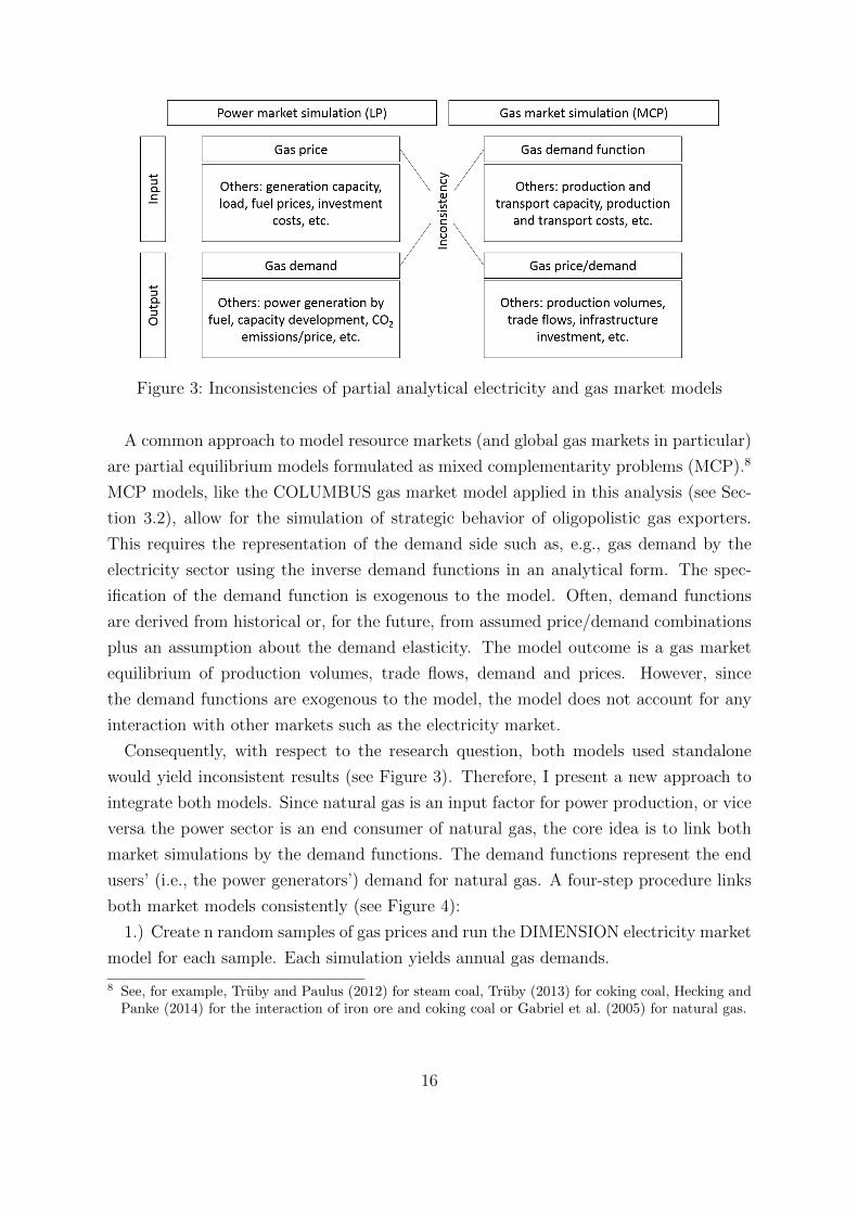
Figure 3: Inconsistencies of partial analytical electricity and gas market models

A common approach to model resource markets (and global gas markets in particular)

are partial equilibrium models formulated as mixed complementarity problems (MCP).8

MCP models, like the COLUMBUS gas market model applied in this analysis (see Sec-

tion 3.2), allow for the simulation of strategic behavior of oligopolistic gas exporters.

This requires the representation of the demand side such as, e.g., gas demand by the

electricity sector using the inverse demand functions in an analytical form. The spec-

ification of the demand function is exogenous to the model. Often, demand functions

are derived from historical or, for the future, from assumed price/demand combinations

plus an assumption about the demand elasticity. The model outcome is a gas market

equilibrium of production volumes, trade flows, demand and prices. However, since

the demand functions are exogenous to the model, the model does not account for any

interaction with other markets such as the electricity market.

Consequently, with respect to the research question, both models used standalone

would yield inconsistent results (see Figure 3). Therefore, I present a new approach to

integrate both models. Since natural gas is an input factor for power production, or vice

versa the power sector is an end consumer of natural gas, the core idea is to link both

market simulations by the demand functions. The demand functions represent the end

users’ (i.e., the power generators’) demand for natural gas. A four-step procedure links

both market models consistently (see Figure 4):

1.) Create n random samples of gas prices and run the DIMENSION electricity market

model for each sample. Each simulation yields annual gas demands.

8 See, for example, Truby and Paulus (2012) for steam coal, Truby (2013) for coking coal, Hecking andPanke (2014) for the interaction of iron ore and coking coal or Gabriel et al. (2005) for natural gas.

16

2.) Use the derived price/demand samples to approximate annual inverse demand

functions p(x) in an analytical form. The resulting demand functions are therefore

outputs of the power market model.

3.) Use the demand functions as inputs of the COLUMBUS gas market model to

derive the oligopolistic gas market equilibrium.

4.) Use the gas market equilibrium prices as inputs of the DIMENSION model and

derive the power market outcome.

Figure 4: Integration of LP power market and MCP gas market model

In the following, the simulation models DIMENSION and COLUMBUS as well as the

model integration approach are explained in greater detail.

3.1. The linear electricity market model DIMENSION

The linear electricity market model DIMENSION9, developed by the Institute of En-

ergy Economics at the University of Cologne, is designed for long-term analyses of the

9 For a detailed model description, see Richter (2011) or Jagemann et al. (2013).

17

European power system up to 2050. As such, DIMENSION and its predecessor DIME

have been backtested and applied in numerous long-term power market studies both in

research (see, e.g., Hagspiel et al. (2014)) and policy advising (see, e.g., Fursch et al.

(2011)).

The model minimizes power system costs by deriving the cost-optimal power plant

dispatch and investment. The power system can be subdivided into different geographi-

cal units such as countries, which are connected by net transfer capacities. Assumptions

on annual power demand are broken down to hourly load patterns of typical days dif-

ferentiated by, e.g., weekend/weekday or summer/winter. The hourly load is assumed

to be inelastic and has to be met by the supply side, i.e., by conventional power plants

and renewables. The hourly feed-in of renewables with zero variable costs such as wind

or solar PV is exogenous to the model and also derived from typical days. The dispatch

of conventional power plants is endogenous to the model and depends on the variable

costs, flexibility and capacity of the power plants. The initial capacity of the generating

units is exogenous to the model, but the model endogenously optimises investment in

new power plants and renewables, depending on investment costs, future power plant

utilization rates and a discount factor.

The DIMENSION model is a useful tool to simulate the effects of different power

market policies in long-term analyses. The EU-ETS, for example, can be modeled by

setting annual CO2 boundaries. If such a boundary is binding, CO2 allowances are

scarce, which fosters power generation by more expensive but less CO2-intensive power

plants. A coal tax can be modeled by increasing the exogenously given coal price, and

a fixed RES bonus can be modeled by reduced or negative variable costs of renewables.

For each parameterization, the model yields the cost-optimal power plant dispatch and

investment decisions, from which other information such as the annual gas demand can

be derived.

3.2. The MCP gas market model COLUMBUS

The MCP gas market model COLUMBUS10 simulates the global gas market up to 2040.

It has been backtested with historic market outcomes in Growitsch et al. (2013). The

model represents the spatial structure of worldwide supply, infrastructure and demand

by a node-edge topology. COLUMBUS derives a market equilibrium by optimizing the

dispatch and investment decisions of several gas market actors such as exporters, traders

or operators of LNG infrastructure or pipelines. Initial production and infrastructure

10For a detailed model description, see Hecking and Panke (2012) or Growitsch et al. (2013).

18

capacities as well as cost parameters are inputs into the model. Actors can, however,

also invest in production and infrastructure at certain investment costs. Concerning the

demand side, the model distinguishes all important demand countries by sector (power,

industry, residential), each represented by annual inverse demand functions. In the basic

COLUMBUS version, demand functions are exogenously defined by historical or, for the

future, by assumed price/demand combinations and assumed price elasticities.

COLUMBUS enables the simulation of Cournot behavior of gas exporters, i.e., the

simulation of a spatial oligopoly. Modeling a Cournot oligopoly in a MCP requires an an-

alytical representation of the price reaction towards changing output. The functions are

common knowledge to all modeled Cournot players. In order to integrate the DIMEN-

SION power market model with COLUMBUS, the annual inverse demand functions of

the power sector are derived by DIMENSION and used in COLUMBUS. The details of

this approach are presented in the next section.

3.3. Integrating power and gas market simulations

Since this study aims at assessing policies with respect to their long-term effects on

power system costs up to 2040, the integrated simulation of electricity and gas market

is conducted for the sample years 2015, 2020, 2030 and 2040.11 Both DIMENSION and

COLUMBUS are inter-temporal models that simulate the investment in power plants

and gas assets, respectively. In particular, there is an important inter-temporal depen-

dency between gas prices and power sector gas demand, illustrated in Figure 5: The gas

prices pi have a direct impact on the dispatch Xi, i.e., the gas consumption of gas-fired

power plants. Additionally, the investment Ii in new gas-fired capacity depends not

only on the future gas prices pi′,(i≤i′) but also on the future utilization of gas-fired plants

Xi,(i≤i′). In turn, the utilization Xi depends on the past investments Ii′,(i≥i′).

11 In order to avoid end effects, the simulation is continued until the year 2070. However, only the modelresults up to 2040 are important for this analysis.

19

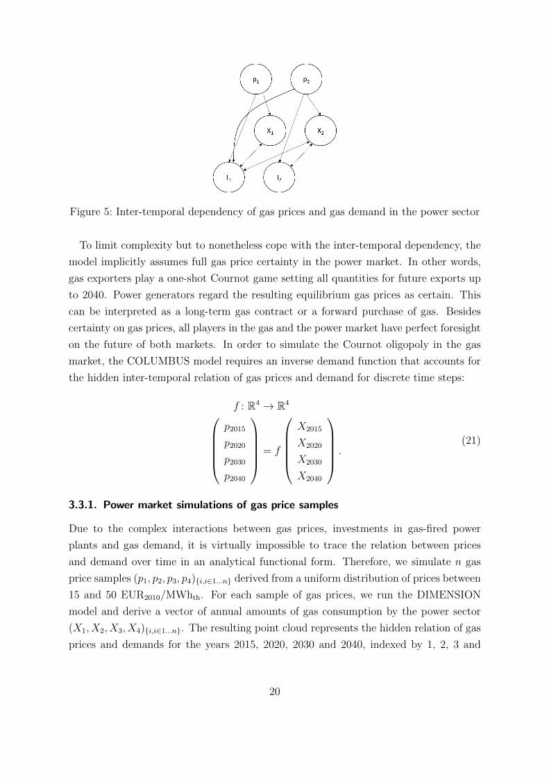
Figure 5: Inter-temporal dependency of gas prices and gas demand in the power sector

To limit complexity but to nonetheless cope with the inter-temporal dependency, the

model implicitly assumes full gas price certainty in the power market. In other words,

gas exporters play a one-shot Cournot game setting all quantities for future exports up

to 2040. Power generators regard the resulting equilibrium gas prices as certain. This

can be interpreted as a long-term gas contract or a forward purchase of gas. Besides

certainty on gas prices, all players in the gas and the power market have perfect foresight

on the future of both markets. In order to simulate the Cournot oligopoly in the gas

market, the COLUMBUS model requires an inverse demand function that accounts for

the hidden inter-temporal relation of gas prices and demand for discrete time steps:

f : R4 → R4p2015

p2020

p2030

p2040

= f

X2015

X2020

X2030

X2040

.(21)

3.3.1. Power market simulations of gas price samples

Due to the complex interactions between gas prices, investments in gas-fired power

plants and gas demand, it is virtually impossible to trace the relation between prices

and demand over time in an analytical functional form. Therefore, we simulate n gas

price samples (p1, p2, p3, p4){i,i∈1...n} derived from a uniform distribution of prices between

15 and 50 EUR2010/MWhth. For each sample of gas prices, we run the DIMENSION

model and derive a vector of annual amounts of gas consumption by the power sector

(X1, X2, X3, X4){i,i∈1...n}. The resulting point cloud represents the hidden relation of gas

prices and demands for the years 2015, 2020, 2030 and 2040, indexed by 1, 2, 3 and

20

4, respectively. In particular, it contains information on how the gas price in one year

reacts to the changing output of a Cournot gas exporter in the same or a different year.

The simulation of a gas market Cournot oligopoly requires the approximation of the

point cloud by an analytical representation.

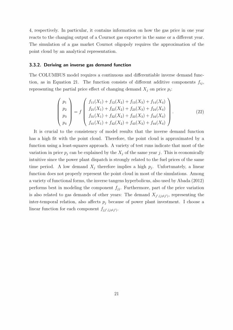
3.3.2. Deriving an inverse gas demand function

The COLUMBUS model requires a continuous and differentiable inverse demand func-

tion, as in Equation 21. The function consists of different additive components fij,

representing the partial price effect of changing demand Xj on price pi:p1

p2

p3

p4

= f

f11(X1) + f12(X2) + f13(X3) + f14(X4)

f21(X1) + f22(X2) + f23(X3) + f24(X4)

f31(X1) + f32(X2) + f33(X3) + f34(X4)

f41(X1) + f42(X2) + f43(X3) + f44(X4)

. (22)

It is crucial to the consistency of model results that the inverse demand function

has a high fit with the point cloud. Therefore, the point cloud is approximated by a

function using a least-squares approach. A variety of test runs indicate that most of the

variation in price pj can be explained by the Xj of the same year j. This is economically

intuitive since the power plant dispatch is strongly related to the fuel prices of the same

time period. A low demand Xj therefore implies a high pj. Unfortunately, a linear

function does not properly represent the point cloud in most of the simulations. Among

a variety of functional forms, the inverse tangens hyperbolicus, also used by Abada (2012)

performs best in modeling the component fjj. Furthermore, part of the price variation

is also related to gas demands of other years: The demand Xj′,(j 6=j′), representing the

inter-temporal relation, also affects pj because of power plant investment. I choose a

linear function for each component fjj′,(j 6=j′).

21

This yields the following inverse demand function:12p1

p2

p3

p4

=

f11(X1) + β12X2 + β13X3 + β14X4

β21X1 + f22(X2) + β23X3 + β24X4

β31X1 + β32X2 + f33(X3) + β34X4

β41X1 + β42X2 + β43X3 + f44(X4)

(23)

with

fii(Xi) = αi +1

γiath(

δi −Xi

δi) (24)

and αi, βij, γi, δi as parameters. The parameter values are optimized in a non-linear

problem with the objective of deriving the demand function that best fits the point cloud

of samples. Therefore, the sum of squared deviations between modeled and sampled

prices is minimized.

3.3.3. Implementing the inverse gas demand function in COLUMBUS

The inverse demand function is used to model a Cournot oligopoly in COLUMBUS. We

assume that there are kk∈K oligopolistic gas exporters supplying a total of Xi in period

i. The term xki is the output of each player k and Cki (xki ) is the respective cost function.

Each player maximizes the following profit function for ii∈1...4 time periods:

maxxki

Πk =4∑i=1

pixki − Ck

i (xki ), with pi = pi(X1, . . . , X4) and Xi =∑k∈K

xki . (25)

12Due to non-linearities, it is beyond the scope of this paper to focus on the mathematical details ofthe function. During the simulation, the derived function leads to consistent results for the gas andpower market and has a good solvability using the PATH-solver in GAMS. Therefore the method ofmodeling the inter-temporal relations of gas prices and gas demand is used in this paper. Also, theinter-temporal approach is presented here since this topic has been hardly addressed in the literaturethus far.

22

Taking the first derivative with respect to xki yields the following first-order condi-

tion (FOC), with λki (xki ) being marginal supply costs, i.e., the player-specific costs of

transport, production and infrastructure scarcity rents:

∂Πk

∂xki= pi +

∑j∈1...4

∂pj∂xki

xki − λki (xki ). (26)

Thus, the FOC takes into account the changing output xki affecting the prices pj of all

time periods. For the specific inverse demand function used in this simulation (Equation

23), the following Karush-Kuhn-Tucker condition is implemented in the model:

−pi −xki(

δi−Xi

δi

)2 (− 1

γiδi

)−∑i 6=j

βjixki + λki (x

ki ) ≥ 0 ⊥ xki ≥ 0. (27)

Besides including the output decision of each player in COLUMBUS, it is necessary to

include the inverse demand function. Two equations are required. The first one balances

the firm-individual output xki and the total output Xi. The total output can also be

interpreted as total demand since in COLUMBUS total annual demand and supply have

to be equal. Therefore, the dual variable is the price pi,∑i

xki = Xi ⊥ pi free . (28)

The second equation balances the price variable pi and the price function depending

on Xj, (j ∈ 1 . . . 4). The dual variable is Xi,

pi = αi +1

γiath(

δi −Xi

δi) +

∑j,j 6=i

βijXj ⊥ Xi free . (29)

23

3.3.4. Deriving the consistent market outcome

Running the COLUMBUS model using the inverse demand function derived from DI-

MENSION yields equilibrium gas prices (p1, p2, p3, p4)∗ and equilibrium gas demand

(X1, X2, X3, X4)∗. The equilibrium gas prices are henceforth used as input fuel prices

for the DIMENSION model. Running DIMENSION yields the total power sector gas

demand (X1, X2, X3, X4). The higher the fit between the gas demand from the COLUM-

BUS and the DIMENSION models, the more consistent the model results with respect to

the interaction of gas and power markets will be. If the fit is insufficient, the procedure

described in this chapter can be rerun with a higher level of detail, i.e., by simulating

more samples (step 1) in a smaller price range around the equilibrium gas prices. If

the fit is sufficient, the DIMENSION market outcome can be assumed to be consistent

to the COLUMBUS outcome and model results such as the power system costs can be

interpreted.13

4. Assumptions and scenarios

4.1. Assumptions on the numerical analysis

The numerical analysis is conducted with a special focus on 11 European countries14

for the time range between 2013 and 2040. Whereas the COLUMBUS model, which

accounts for the entire global gas market, is only run once per scenario, the electricity

market model DIMENSION has to be run once for each gas price sample, i.e., 1000

times per scenario.15 In order to reduce the complexity of DIMENSION and decrease

computation time, the number of simulated countries is hence limited to 11. In total,

these countries make up for 75 % of current CO2 emissions of the European power

sector and half of the current EU-ETS allowances. Since this study focuses on the

power sector, other EU-ETS sectors such as cement production are not included in

the modeling. Thus, this approach implicitly assumes the same marginal costs for the

13Appendix A provides an assessment of the convergence of the COLUMBUS and the DIMENSIONmodels and shows how the outlined mechanism, i.e., simulating more samples in a smaller price range,improves the convergence of both models.

14These countries include Austria, Belgium, Czech Republic, Denmark, France, Germany, Great Britain,Italy, Poland, the Netherlands and Switzerland. The choice of these 11 countries was made becauseof their importance concerning European CO2 emissions, their location in the center of Europe andtheir high gas market integration.

15The number of samples is set to 1000 in this analysis, with results achieving consistent results of gasand power market models.

24

proportional CO2 reduction of other EU-ETS sectors. Although this is clearly a strong

assumption, it does not qualitatively change the main messages of this analysis.

In this analysis, the DIMENSION model assumes an emissions quota of roughly 200

million CO2 allowances for the power sector of the 11 countries in 2050, which equals a

80% CO2 reduction compared to 2012. The number of allowances is reduced proportion-

ately over time between 2012 and 2050. The analysis assumes implicitly that emissions

certificates can be traded among those 11 countries. The quota must be achieved for each

year, i.e., the possibility of “banking and borrowing” is excluded. In the basic configu-

ration of this research, any other climate policy such as national RES subsidies or RES

targets are, in contrast to the current regulation, not included in the simulation. Con-

cerning the power plant and renewables data, this analysis uses the large-scale database

of the Institute of Energy Economics at the University of Cologne, which contains in-

formation on ca. 4700 power plants – almost the entire European generation capacity

including renewables. The database includes a variety of power plant parameters such

as age, lifetime, efficiency, ramp-up times and current investment and operational costs.

Concerning future investment costs, the assumption is made that the investment costs

for mature technologies are constant, whereas costs decrease for new technologies such

as certain renewables. Future investment costs are mainly based on IEA (2013).

Concerning fuel prices, this analysis is consistent with to the assumptions made in

Fursch et al. (2011), with the exception of gas prices which are modeled endogenously. In

contrast, coal prices are exogenous to the model for three reasons: First, there is currently

no dominant player active on the global thermal coal market. Thus, a polypolistic coal

market can be assumed (see, e.g., Truby and Paulus (2012) or Haftendorn and Holz

(2010)). Second, whereas for many natural gas exporters the only sales opportunity

is Europe via pipeline, coal trade via ship or train is much more flexible concerning

the demand side. Third, due to the huge mining capacities in China (in particular),

the global coal supply curve is rather flat. If European coal imports were to decline,

traditional coal exporters such as Colombia or Russia could easily shift their exports to

China or India, where they would crowd out domestic production. Although European

coal prices would decrease after a demand drop, the price effect would be negligible

compared to natural gas.

The gas market model COLUMBUS accounts for all major production and demand re-

gions worldwide. The above-mentioned 11 countries are regarded as one demand region.

Therefore, an implicit assumption is made that there is a full gas market integration

among these countries, which is reasonable considering the well-built transport infras-

25

tructure, in particular, of the Northwest European gas market. The annual exogenous

demand of these 11 countries, which is composed of the sectoral demand for power,

heat and industry, is corrected for the power demand. The power demand is modeled by

the demand functions derived through DIMENSION. The heat and industry gas demand

functions are assumed to be exogenous. These assumptions as well as the future demand

for other countries worldwide follow the WEO 2013 and MTGMR 2013. Parameters on

existing infrastructure and production capacities are identical to those of Growitsch et al.

(2013), in which the authors provide a calibration of the model based on historic data.

Future production and infrastructure capacities are derived endogenously in the model.

However, to account for political or geographical limitations or the resource endowment

of supply countries, potential investment in production and infrastructure assets are lim-

ited, in line with the future projections of WEO 2013. Two assumptions are of particular

importance for the degree of competition in Europe: First, potential LNG exports from

the US and Canada amount to 60 bcm for 2020 and 200 bcm for 2040.16 Second, gas

trade from Iran and Iraq via Turkey to Europe is excluded.17 More detailed informa-

tion concerning model parameters of the DIMENSION and COLUMBUS models are

provided in Appendix C.

4.2. Scenario design

To investigate the hypotheses H1 to H3, the paper at hand assesses three scenarios of dif-

ferent climate policy regimes in the European power sector. In the scenario “Reference”,

the only active carbon abatement policy is the EU-ETS. In particular and in contrast to

the current real-world regulation, there are no additional RES subsidies such as national

feed-in-tariffs in place. The scenario “Coal Tax (CT)” assumes the presence of a coal

tax in addition to the EU-ETS. The coal tax is raised for each thermal megawatt-hour

of hard coal burned to generate power. The tax is identical for each of the countries

considered. A tax of 10 EUR2010/MWhth and a tax of 20 EUR2010/MWhth are simulated.

The scenario “Fixed RES Bonus (FB)” assumes a fixed bonus subsidy that is paid to

the operator of a renewable power plant for each megawatt-hour of electricity generated.

16The parameter “potential LNG exports” is an upper boundary on the capacity of LNG export ter-minals. Hence, this parameter does not necessarily match the exports derived by the model sincethe model could regard investment or LNG exports to be uneconomical. Furthermore, LNG exportsfrom North America would not necessarily affect the European gas market, since they could also beattracted by Asian importers.

17Even though Iran and Iraq are endowed with substantial natural gas resources, future gas salesto Europe are highly uncertain due to the current political situation and the need for transportinfrastructure.

26

The fixed bonus is independent of technology and location. Fixed bonus subsidies of 5,

10, 20 and 30 EUR2010/MWhel are simulated.

In order to examine hypothesis H4, each of the three scenarios is derived in an addi-

tional variant that assumes a different market structure of the gas market: In a fictitious

case, I assume a cartel of Norway and Russia. Even though this assumption is not nec-

essarily realistic from a gas market point of view, the sole purpose of this setting is to

assess the effects of a higher degree of market power.

5. Results of the numerical analysis

The simulation results are discussed in four parts: First, I focus on the effects of climate

policies on the power market gas demand functions and the resulting equilibrium gas

prices. Secondly, the policy effects on power generation by fuel type are discussed.

Thirdly, I compare the overall power system costs of the different scenarios with a

special focus on the cost effects as discussed in Section 2.3. Fourth, I analyze the effects

of changing gas market power on the power system costs.

5.1. Gas demand functions and equilibrium gas prices

Figure 6 shows the effects of renewable subsidies on gas demand functions for the years

2015, 2020, 2030 and 2040. “REF” labels reference scenario and “FB10” and “FB20” la-

bel a fixed bonus payment of 10 EUR2010/MWhel and 20 EUR2010/MWhel, respectively.

The point clouds illustrate gas price/demand combinations simulated by the power mar-

ket model DIMENSION. The black lines show the approximated demand functions.18

The yellow square shows the equilibrium gas price/demand combination for the respec-

tive year and scenario resulting from the gas market simulation by the COLUMBUS

model.

18Since the demand function for each scenario is four-dimensional, the dimensionality has to be reducedin order to show it graphically. For the year 2015, for example, the function drawn shows the relationbetween the gas price and the quantity of the year 2015. In this figure, the other quantities for theyears 2020, 2030 and 2040 are set to the resulting gas market equilibrium quantities.

27

Figure 6: Gas price/demand samples, demand curves and gas market equilibria for thefixed bonus scenarios

The figure shows a similar effect for all four years. Increasing the renewable sub-

sidy shifts the gas demand function inwards. In other words, increasing competition by

cheaper renewables decreases the willingness-to-pay for natural gas of the power sector.

The shift in the demand curve changes the resulting gas market equilibrium. An in-

creasing fixed bonus for renewables increases the equilibrium gas demand and decreases

gas prices. This effect is unambiguous for all subsidy scenarios and all years although

the price decrease is very weak for the year 2020.

Figure 7 is identical to figure 6 but illustrates the effects of a coal tax on the gas demand

functions and the resulting gas market equilibria. “CT10” and “CT20” label coal tax

scenarios of 10 EUR2010/MWhth and 20 EUR2010/MWhth, respectively. In particular for

the years 2015 and 2020, fuel competition between coal and natural gas becomes more

intensive because of the coal tax. For this reason, in CT10 and CT20, the power sector

becomes very sensitive with regard to natural gas prices. Even though gas demand in

equilibrium increases substantially, the gas price decreases. This can be explained by

lower oligopoly markups of gas producers because of the less steep and more price elastic

demand function induced by the coal tax. For the years 2030 and 2040 the elasticity is

28

not affected as much. Thus, the gas market equilibria show that gas consumption and

gas prices increase with the coal tax.

Figure 7: Gas price/demand samples, demand curves and gas market equilibria for coaltax scenarios

With regard to hypothesis H1, the results confirm the intuition that renewable subsi-

dies cause a decrease in gas prices. Concerning the coal tax the picture is more diffuse.

Although in 2030 and 2040 a coal tax causes an increase in gas prices, the example of

the year 2015 has provided a valuable exception: If a policy significantly changes the

gas demand elasticity, the resulting price effect can contradict to H1 because of the

oligopolistic gas market structure.

5.2. Effects of climate policies on power generation

Figure 8 depicts the effects on power generation by fuel type when a fixed bonus of 20

EUR2010/MWhel for renewables is introduced. As shown in Section 2, such a subsidy

has both a direct effect (labeled “Dir.”) and an indirect effect (labeled “Ind.”) on power

generation. The direct effect is derived by comparing the power generation of the Ref-

erence scenario xREF (gREF ) with the power generation of the fixed RES Bonus scenario

29

(FB), but applying the equilibrium gas prices of the Reference scenario (xFB20(gREF )).

Thus,

xdir = xFB20(gREF )− xREF (gREF ). (30)

The indirect effect, which is induced by a changing gas market price, is derived by

comparing xFB20(gREF ) to xFB20(gFB20). Thus,

xind = xFB20(gFB20)− xFB20(gREF ). (31)

Figure 8: Effects of a fixed RES bonus on power generation by fuel type

As expected from the stylized model described in Section 2, the direct effect of a

subsidy under the EU-ETS is an increasing generation of renewables and cheap, but

CO2-intensive, coal and lignite. Gas-fired generation decreases. As discussed in Section

5.1, gas prices in equilibrium decrease when a subsidy is introduced. Therefore, the

indirect effect of a subsidy via the gas price is an increasing gas-fired generation, whereas

generation from renewables, coal and lignite decreases. However, the overall effect is a

decreasing gas-fired generation.

Figure 9 illustrates the effects of a 10 EUR2010/MWhth coal tax on power generation.

The direct effect of a coal tax is a fuel switch from coal to gas. It can be observed that

renewable generation also decreases, for example in 2020. Since coal-fired generation is

30

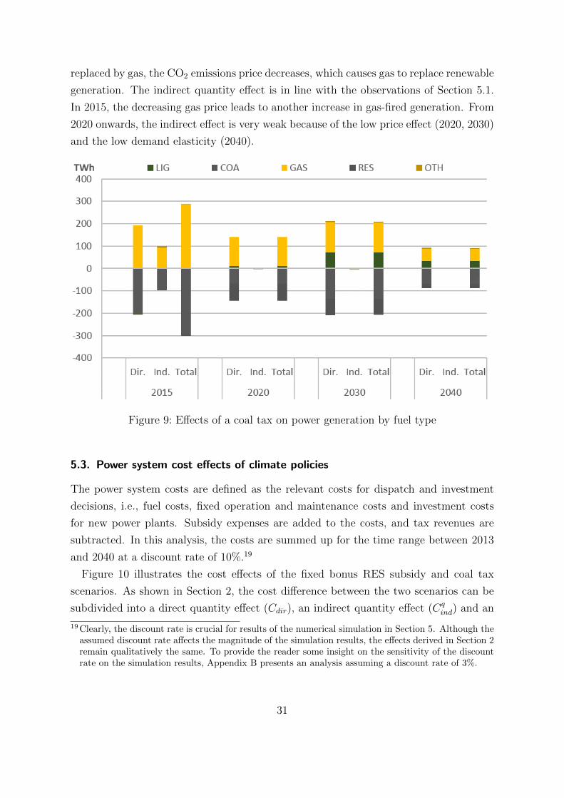
replaced by gas, the CO2 emissions price decreases, which causes gas to replace renewable

generation. The indirect quantity effect is in line with the observations of Section 5.1.

In 2015, the decreasing gas price leads to another increase in gas-fired generation. From

2020 onwards, the indirect effect is very weak because of the low price effect (2020, 2030)

and the low demand elasticity (2040).

Figure 9: Effects of a coal tax on power generation by fuel type

5.3. Power system cost effects of climate policies

The power system costs are defined as the relevant costs for dispatch and investment

decisions, i.e., fuel costs, fixed operation and maintenance costs and investment costs

for new power plants. Subsidy expenses are added to the costs, and tax revenues are

subtracted. In this analysis, the costs are summed up for the time range between 2013

and 2040 at a discount rate of 10%.19

Figure 10 illustrates the cost effects of the fixed bonus RES subsidy and coal tax

scenarios. As shown in Section 2, the cost difference between the two scenarios can be

subdivided into a direct quantity effect (Cdir), an indirect quantity effect (Cqind) and an

19Clearly, the discount rate is crucial for results of the numerical simulation in Section 5. Although theassumed discount rate affects the magnitude of the simulation results, the effects derived in Section 2remain qualitatively the same. To provide the reader some insight on the sensitivity of the discountrate on the simulation results, Appendix B presents an analysis assuming a discount rate of 3%.

31

indirect price effect (Cpind). In the example of the scenario FB20, the direct quantity

effect is derived by comparing the costs of scenario FB20 with the Reference scenario,

with both scenarios assuming the gas price of the Reference scenario, gREF :

Cdir = CFB20(gREF )− CREF (gREF ). (32)

The sum of the indirect quantity effect and the indirect price effect is derived by

comparing the costs of the FB20 scenario using the price of the Reference scenario,

CFB20(gREF ), to the costs of the FB20 scenario using the gas price of the FB20 scenario,

CFB20(gFB20). Thus,

Cxind + Cp

ind = CFB20(gFB20)− CFB20(gREF ). (33)

The indirect price effect is derived as the gas price difference between scenario FB20

and the Reference scenario multiplied by the gas consumption of the power sector in the

FB20 scenario, xFB20G :

Cpind = (gFB20 − gREF )xFB20

G . (34)

As discussed in the previous section a coal tax in the power sector causes a deviation

from the cost efficient power generation under the no-tax case. Hence, the direct cost

effect of a coal tax is positive, as Figure 10 illustrates. In the CT10 scenario, where a coal

tax causes gas prices to both increase and decrease (depending on the year), the indirect

quantity effect is positive. In other words, changing gas prices forces power generation

to deviate from the cost-optimal generation even more than seen in the direct effect.

However, the costs of gas purchases decrease, i.e., the indirect price effect reduces costs.

Yet, in total, power system costs in the CT10 scenario are higher than in the reference

case. In the CT20 scenario, except for the year 2015, gas prices increase. Therefore,

a higher gas price increases the costs of gas purchased by the power sector, i.e., the

indirect price effect is positive. Hence, these numerical results confirm hypothesis H2:

A coal tax increases overall power system costs.

32

Figure 10: Power system cost effects of different levels of coal taxes and RES subsidies

With regard to fixed bonus RES subsidies, Figure 10 reveals that the direct cost effect

of such a subsidy is positive and increases with the subsidy. However, since the subsidy

causes the gas price to decrease, the indirect quantity effect reduces the additional costs

incurred by the direct quantity effect. Nonetheless, the sum of both the direct and

indirect quantity effect is positive. However, the indirect price effect of a subsidy, i.e.,

decreasing costs of gas purchased by the power sector, overcompensates the quantity

effects. Therefore, this numerical simulation of the European power and gas market

confirms hypothesis H3: A fixed bonus RES subsidy may decrease overall power system

costs because of the gas price reaction.

5.4. Cost effects of supply side concentration on the gas market

A higher supply side concentration on the gas market is simulated by a fictitious cartel

of Norway and Russia. For the scenarios FB20 and the CT10, Figure 11 compares

the gas price reaction (i.e., the price differences to the respective REF scenario) under

the standard gas market structure (STANDARD) with the cartel (CARTEL).20 The

gas price reduction in the FB20 scenario is higher in the case of the cartel than in the

standard case for each year. In the Coal Tax scenario CT10, the gas price reduction in

20For the other scenarios, the results are qualitatively the same.

33

the cartel case is lower in 2015 than in the standard case, whereas the gas price increase

in the years 2020 and 2030 is higher.

Figure 11: Gas price effects of different policies under different gas supply-side marketstructures

These price reactions explain the cost effects when different gas supply-side structures

are assumed (see Figure 12). In the RES subsidy scenarios, the higher price decrease

causes a higher indirect price effect such that the overall power system cost reduction

is higher in the CARTEL case than in the STANDARD case. In the coal tax scenarios,

the opposite holds. To sum up, with regard to hypothesis H4, a higher market power in

the gas market amplifies the discussed effects.

34

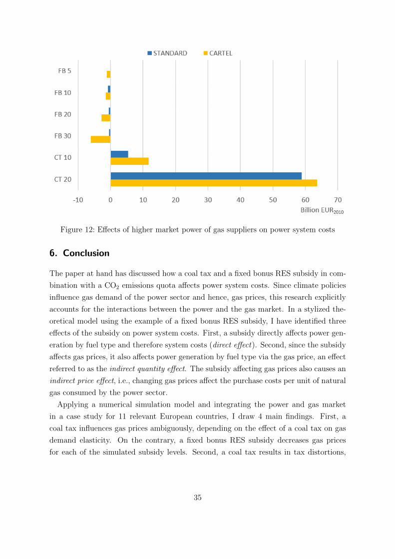
Figure 12: Effects of higher market power of gas suppliers on power system costs

6. Conclusion

The paper at hand has discussed how a coal tax and a fixed bonus RES subsidy in com-

bination with a CO2 emissions quota affects power system costs. Since climate policies

influence gas demand of the power sector and hence, gas prices, this research explicitly

accounts for the interactions between the power and the gas market. In a stylized the-

oretical model using the example of a fixed bonus RES subsidy, I have identified three

effects of the subsidy on power system costs. First, a subsidy directly affects power gen-

eration by fuel type and therefore system costs (direct effect). Second, since the subsidy

affects gas prices, it also affects power generation by fuel type via the gas price, an effect

referred to as the indirect quantity effect. The subsidy affecting gas prices also causes an

indirect price effect, i.e., changing gas prices affect the purchase costs per unit of natural

gas consumed by the power sector.

Applying a numerical simulation model and integrating the power and gas market

in a case study for 11 relevant European countries, I draw 4 main findings. First, a

coal tax influences gas prices ambiguously, depending on the effect of a coal tax on gas

demand elasticity. On the contrary, a fixed bonus RES subsidy decreases gas prices

for each of the simulated subsidy levels. Second, a coal tax results in tax distortions,

35

i.e., it increases power system costs even at constant gas prices (direct effect). Since

a coal tax affects gas prices ambiguously, the overall power system costs increase, even

when accounting for the indirect quantity and price effects. Third, the simulation results

reveal that a fixed bonus RES subsidy can decrease overall power system costs: On the

one hand, the subsidy increases costs given fixed gas prices (direct effect); yet, on the

other hand, the subsidy decreases gas prices such that the indirect quantity and price

effects overcompensate the direct effect. Fourth, when a higher level of market power of

gas suppliers is assumed, the overall effect of higher market power on power system costs

is amplified. Concerning a coal tax, the simulation results show that a higher degree

of market power further increases costs, whereas, concerning a RES subsidy, it further

decreases costs. The assumed discount rate of future costs has proven to be a crucial

parameter, which affects these results quantitatively, however not qualitatively.

This analysis has focused solely on the effects of climate policies on the power system

costs of 11 select European countries. In particular, decreasing power system costs

through a fixed RES bonus do not imply that this subsidy makes CO2 abatement more

efficient. The reason for decreasing power system costs are the decreasing expenditures

of power utilities for the gas purchased, which come at the disadvantage of gas suppliers,

whose revenues decline. In other words, introducing the subsidy redistributes welfare

from players in the gas market to players or end consumers in the power market, as well as

to suppliers of coal or renewable technologies. Even though the discussed subsidy would

cause an inefficient allocation of primary energy use in the power sector and, hence,

higher CO2 abatement costs, European policy makers could have a sound motivation

to establish a fixed RES bonus subsidy: in order to redistribute welfare from the most

important gas suppliers such as Russia, Norway, Algeria or Qatar to market participants

of the European power market, i.e., power producers or end users.

This research has pointed out that the evaluation of climate policies in the power

sector should take into account the upstream markets and their market structure. The

main focus was a discussion of the power system cost effects of climate policies in due

consideration of the interdependencies of the power and gas market. Yet, it is important

to stress that this study does not provide a comprehensive assessment of climate policies,

for several reasons. First, the sole objective of this study is to determine the minimal

power system costs. Regarding the coal tax, the tax could aim at further objectives

other than efficient CO2 abatement. Other policy objectives could justify higher costs

from a coal tax. Second, this research only assesses two policies and simulates a setting

in which there are no other climate policies in place. In reality, there is a variety

36

of (national) climate policies which could affect gas prices differently or interact with

other policies. In particular, the study does not say that the current regime of national

technology-specific RES subsidies decreases power system costs. Third, even though

the study reveals cost reduction potentials of a technology-neutral and location-neutral

RES subsidy, it remains an open question whether there may be another policy regime

that further decreases gas prices and, therefore, power system costs. As such, an EU

energy union is often discussed as a mean to decrease gas purchasing costs. However,

the main flaw of such a measure, the threat of downstream cartelization, is avoided by a

RES subsidy. Fourth, the dynamic effects of climate policies, such as a higher or lower

technological progress because of a subsidy, are not investigated in this research. Fifth,

efficiency gains and losses in other related markets such as the gas, coal or renewables

market have not been assessed. All of the five outlined aspects could motivate interesting

extensions to this paper.

37

References

Abada, I., 2012. Modelisation des marches du gaz naturel en europe en concurrenceoligopolistique: le modele gammes et quelques applications.

Bennear, L. S., Stavins, R. N., 2007. Second-best theory and the use of multiple policyinstruments. Environmental and Resource Economics 37 (1), 111–129.

Bohringer, C., Koschel, H., Moslener, U., 2008. Efficiency losses from overlapping regu-lation of eu carbon emissions. Journal of Regulatory Economics 33 (3), 299–317.

Bohringer, C., Rosendahl, K. E., 2011. Greening electricity more than necessary: on thecost implications of overlapping regulation in eu climate policy.

del Rıo Gonzalez, P., 2007. The interaction between emissions trading and renewableelectricity support schemes. an overview of the literature. Mitigation and adaptationstrategies for global change 12 (8), 1363–1390.

Fischer, C., Preonas, L., et al., 2010. Combining policies for renewable energy: Is thewhole less than the sum of its parts. International Review of Environmental andResource Economics 4 (1), 51–92.

Fursch, M., Lindenberger, D., Malischek, R., Nagl, S., Panke, T., Truby, J., 2011.German nuclear policy reconsidered: Implications for the electricity market. EWIWorking Paper 11/12, Koln.URL http://hdl.handle.net/10419/74404

Gabriel, S., Kiet, S., Zhuang, J., 2005. A mixed complementarity-based equilibriummodel of natural gas markets. Operations Research 53 (5), 799.

Growitsch, C., Hecking, H., Panke, T., 2013. Supply disruptions and regional price effectsin a spatial oligopoly-an application to the global gas market.

Haftendorn, C., Holz, F., 2010. Modeling and analysis of the international steam coaltrade. The Energy Journal 31 (4), 205–229.

Hagspiel, S., Jagemann, C., Lindenberger, D., Brown, T., Cherevatskiy, S., Troster, E.,2014. Cost-optimal power system extension under flow-based market coupling. Energy66 (0), 654 – 666.URL http://www.sciencedirect.com/science/article/pii/S0360544214000322

Hecking, H., Panke, T., 2012. COLUMBUS - a global gas market model. EWI WorkingPaper 12/06.

Hecking, H., Panke, T., 2014. Quantity-setting oligopolies in complementary inputmarkets-the case of iron ore and coking coal.

Huppmann, D., Egging, R., 2014. Market power, fuel substitution and infrastructure: Alarge-scale equilibrium model of global energy markets.

38

IEA, 2013. World Energy Outlook 2013. International Energy Agency, Paris.

Jagemann, C., Fursch, M., Hagspiel, S., Nagl, S., 2013. Decarbonizing europe’s powersector by 2050 – analyzing the economic implications of alternative decarbonizationpathways. Energy Economics 40 (0), 622 – 636.URL http://www.sciencedirect.com/science/article/pii/S0140988313001928

Lienert, M., Lochner, S., 2012. The importance of market interdependencies in modelingenergy systems–the case of the european electricity generation market. InternationalJournal of Electrical Power & Energy Systems 34 (1), 99–113.

Newbery, D. M., 2008. Climate change policy and its effect on market power in the gasmarket. Journal of the European Economic Association 6 (4), 727–751.

Richter, J., 2011. Dimension-a dispatch and investment model for european electricitymarkets.

Sijm, J., 2005. The interaction between the eu emissions trading scheme and nationalenergy policies. Climate Policy 5 (1), 79–96.

Sorrell, S., Sijm, J., 2003. Carbon trading in the policy mix. Oxford Review of EconomicPolicy 19 (3), 420–437.

Tinbergen, J., 1952. On the theory of economic policy.

Truby, J., 2013. Strategic behaviour in international metallurgical coal markets. EnergyEconomics 36, 147–157.

Truby, J., Paulus, M., 2012. Market structure scenarios in international steam coal trade.The Energy Journal Volume 33 (Number 3).URL http://EconPapers.repec.org/RePEc:aen:journl:33-3-04

39

A. Convergence of the power and the gas market model

In order to assess the convergence of the power market model and the gas market model,

equilibrium gas prices and gas demand of both models are compared in this section. Since

the equilibrium gas prices of the gas market model are used as an input to the power

market model, gas prices are identical in both models. Therefore, the convergence of

both models is assessed by comparing the equilibrium gas demand of the power market

model and the gas market model.

Table A lists the deviation of gas demands of both models for different scenarios. The

deviation d is derived as follows: d = xdimxcol− 1, with xdim being the equilibrium gas

demand derived by the DIMENSION model and xcol being the equilibrium gas demand

derived by the COLUMBUS model. The worst convergence of both models is observed

for the years 2015 and 2020 and the scenarios FB20 and FB30 with deviations of up to

10%.

Table 1: Deviation of gas demands between power market model and gas market modelwith different price ranges

Scenario 2015 2020 2030 2040

REF 5% -2% -1% 0%FB5 3% -1% -2% 1%FB10 0% -1% -2% 1%FB20 -5% -3% -4% 1%FB30 -5% -10% -7% 3%CT10 5% -2% 3% 1%CT20 5% 2% 1% -1%

One approach to improve the consistency of both models could be to use a different

functional shape of the inverse demand function for a certain year, e.g., a hyperbolic

function. Another approach could be to focus the range of gas price samples to a

smaller interval, i.e., increasing the fit in the region of prices that were relevant during

the gas price simulation. Consequently, instead of sampling gas prices between 15 and 50

EUR2010/MWhth for all years, I limit the price range to 15 to 25 EUR2010/MWhth for the

year 2015, to 20 to 30 EUR2010/MWhth for the year 2020 and to 25 to 40 EUR2010/MWhth

for the years 2030 and 2040. The gas demand function is estimated once more based

on the restricted set of samples, and new equilibria of both models are derived. Table

A lists the resulting gas demand deviations between both models. The results reveal

that the outlined approach has improved the convergence of both models. The results

40

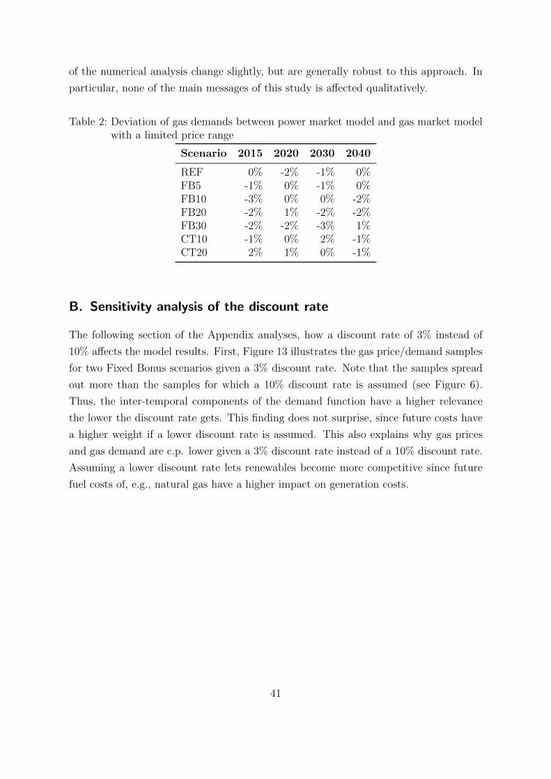
of the numerical analysis change slightly, but are generally robust to this approach. In

particular, none of the main messages of this study is affected qualitatively.

Table 2: Deviation of gas demands between power market model and gas market modelwith a limited price range

Scenario 2015 2020 2030 2040

REF 0% -2% -1% 0%FB5 -1% 0% -1% 0%FB10 -3% 0% 0% -2%FB20 -2% 1% -2% -2%FB30 -2% -2% -3% 1%CT10 -1% 0% 2% -1%CT20 2% 1% 0% -1%

B. Sensitivity analysis of the discount rate

The following section of the Appendix analyses, how a discount rate of 3% instead of

10% affects the model results. First, Figure 13 illustrates the gas price/demand samples

for two Fixed Bonus scenarios given a 3% discount rate. Note that the samples spread

out more than the samples for which a 10% discount rate is assumed (see Figure 6).

Thus, the inter-temporal components of the demand function have a higher relevance

the lower the discount rate gets. This finding does not surprise, since future costs have

a higher weight if a lower discount rate is assumed. This also explains why gas prices

and gas demand are c.p. lower given a 3% discount rate instead of a 10% discount rate.

Assuming a lower discount rate lets renewables become more competitive since future

fuel costs of, e.g., natural gas have a higher impact on generation costs.

41

Figure 13: Gas price/demand samples, demand curves and gas market equilibria for theFixed Bonus scenarios at a discount rate of 3%

Figure 14 depicts the cost effects of the Fixed Bonus and Coal Tax scenarios when

assuming a discount rate 3%. Similar effects as in the 10% discount rate case can be

observed, i.e., the overall cost effect of a coal tax is positive and (except for the FB30

scenario) it is negative for the Fixed Bonus scenarios. However, effects strongly differ in

magnitude due to the lower discount rate of 3%.

42

Figure 14: Power system cost effects of different levels of coal taxes and RES subsidiesat a discount rate of 3%

C. Data

Table 3: Fuel costs for power generation

EUR2010/MWhth 2015 2020 2030 2040

Nuclear 3.5 3.3 3.3 3.3Lignite 1.4 1.4 2.7 2.7Coal 9.1 10.1 10.9 11.9Oil 42.5 47.6 58.0 69.0

43

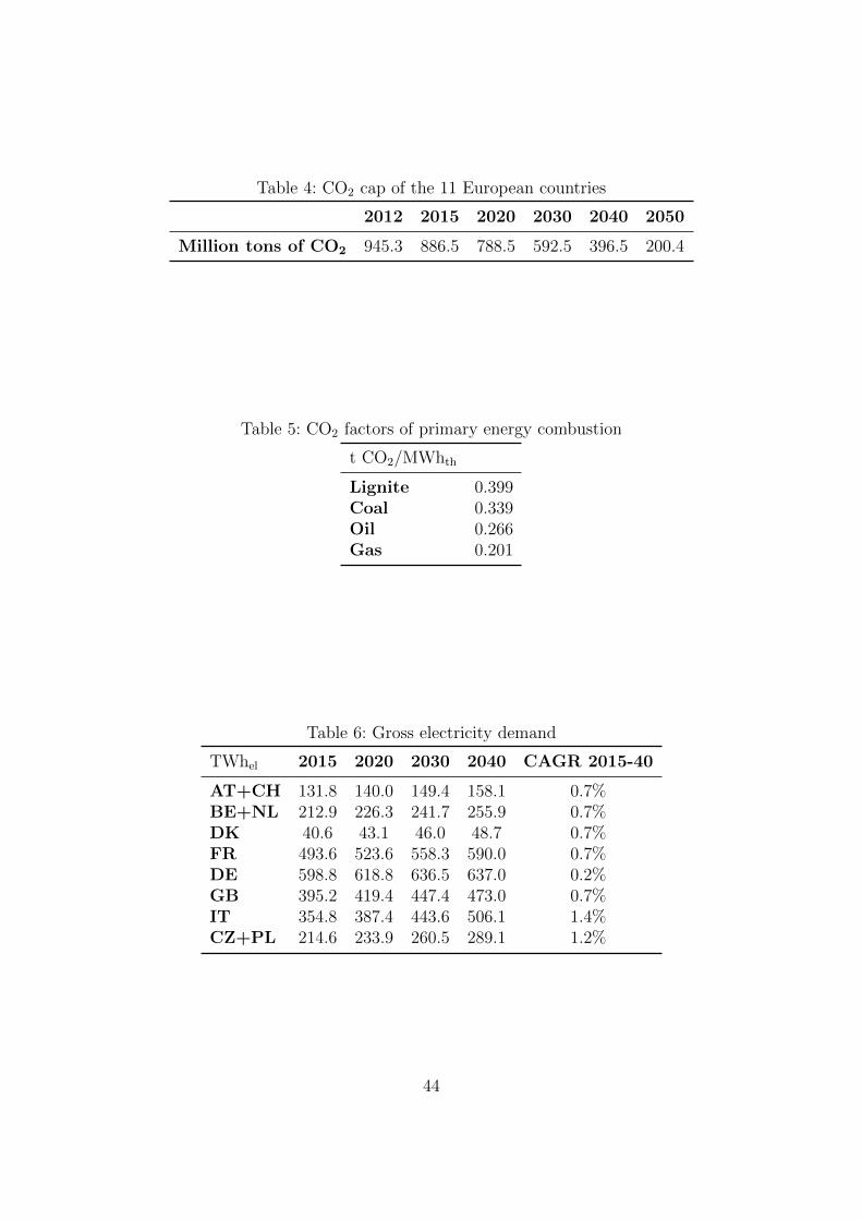
Table 4: CO2 cap of the 11 European countries

2012 2015 2020 2030 2040 2050

Million tons of CO2 945.3 886.5 788.5 592.5 396.5 200.4

Table 5: CO2 factors of primary energy combustion

t CO2/MWhth

Lignite 0.399Coal 0.339Oil 0.266Gas 0.201

Table 6: Gross electricity demand

TWhel 2015 2020 2030 2040 CAGR 2015-40

AT+CH 131.8 140.0 149.4 158.1 0.7%BE+NL 212.9 226.3 241.7 255.9 0.7%DK 40.6 43.1 46.0 48.7 0.7%FR 493.6 523.6 558.3 590.0 0.7%DE 598.8 618.8 636.5 637.0 0.2%GB 395.2 419.4 447.4 473.0 0.7%IT 354.8 387.4 443.6 506.1 1.4%CZ+PL 214.6 233.9 260.5 289.1 1.2%

44

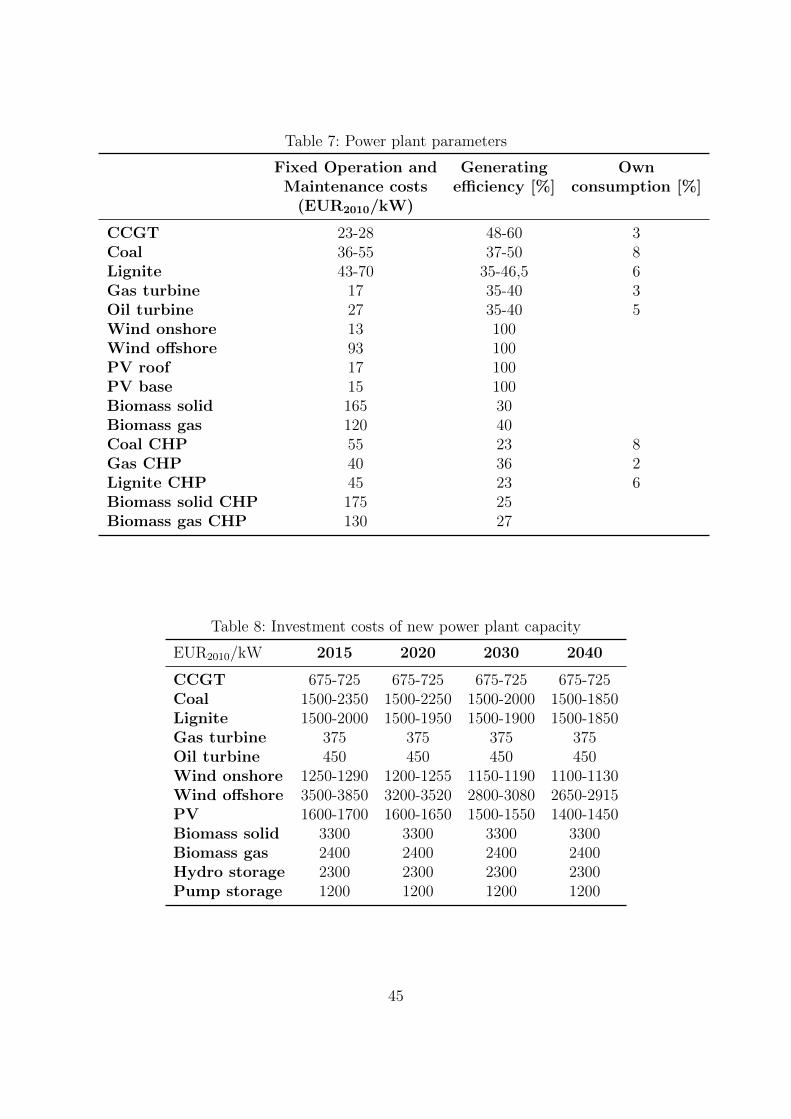
Table 7: Power plant parameters

Fixed Operation and Generating OwnMaintenance costs efficiency [%] consumption [%]

(EUR2010/kW)

CCGT 23-28 48-60 3Coal 36-55 37-50 8Lignite 43-70 35-46,5 6Gas turbine 17 35-40 3Oil turbine 27 35-40 5Wind onshore 13 100Wind offshore 93 100PV roof 17 100PV base 15 100Biomass solid 165 30Biomass gas 120 40Coal CHP 55 23 8Gas CHP 40 36 2Lignite CHP 45 23 6Biomass solid CHP 175 25Biomass gas CHP 130 27

Table 8: Investment costs of new power plant capacity

EUR2010/kW 2015 2020 2030 2040

CCGT 675-725 675-725 675-725 675-725Coal 1500-2350 1500-2250 1500-2000 1500-1850Lignite 1500-2000 1500-1950 1500-1900 1500-1850Gas turbine 375 375 375 375Oil turbine 450 450 450 450Wind onshore 1250-1290 1200-1255 1150-1190 1100-1130Wind offshore 3500-3850 3200-3520 2800-3080 2650-2915PV 1600-1700 1600-1650 1500-1550 1400-1450Biomass solid 3300 3300 3300 3300Biomass gas 2400 2400 2400 2400Hydro storage 2300 2300 2300 2300Pump storage 1200 1200 1200 1200

45