BUILDING THE COST CURVES FOR THE INDUSTRIAL SOURCES … Non-CO2 Gase… · abatement cost curve for...

BUILDING THE COST CURVES FOR THE INDUSTRIAL SOURCES OF NON-CO2

GREENHOUSE GASES

Report Number PH4/25 October 2003

This document has been prepared for the Executive Committee of the Programme. It is not a publication of the Operating Agent, International Energy Agency or its Secretariat.

i

BUILDING THE COST CURVES FOR THE INDUSTRIAL SOURCES OF NON-CO2 GREENHOUSE GASES

Background to the Study

The Non-CO2 gases taken together have made about half as much contribution as CO2 to climate change since pre-industrial times. Their atmospheric concentrations are significantly lower than CO2 but are substantially more powerful greenhouse gases than CO2, over a typical time period such as 100 years. In any assessment of greenhouse gas abatement strategy, the impact of reducing Non-CO2 greenhouse gas emissions must be carefully considered. One way of comparing the mitigation options is to develop abatement cost curves1 for the Non-CO2 greenhouse gases that allow direct comparison with similar curves for CO2 abatement options. This could be done by developing abatement curves on a CO2 equivalent2 (CO2 eq.) basis, which takes allowance of the different global warming potentials (GWPs) of these gases. The IEA Greenhouse Gas R&D Programme (IEA GHG) has carried out a series of studies covering all of the Non-CO2 greenhouse gases (except those covered by the Montreal Protocol3). In Phase 2, a series of studies were undertaken to assess the abatement options for methane (CH4), whilst in Phase 3, the abatement options for nitrous oxide (N2O) and the engineered chemicals4 were assessed. In both the phase 3 studies, although these had not been attempted for some of the Phase 2 methane studies because there was insufficient information available at that time. However, it is now considered that sufficient further research effort has been expended that will allow the abatement cost curves for all of these sectors to be developed. The aim of this study is to update the abatement potential and cost data presented in the earlier studies on Non-CO2 greenhouse gases and to develop abatement cost curves for all the Non-CO2 gases on a common basis. However, the scope of the study was limited to the industrial sectors only because, it is considered by IEA GHG, that, there is still insufficient data available on the costs associated with the abatement of the “other anthropogenic sources” that arise from agricultural production to allow an abatement cost curve to be developed at this time. The study has been carried out by ICF Consulting of the USA.

Results and Discussion The following areas are discussed in this report:

• Scope of study and methodology adopted, • Global emissions of Non-CO2 greenhouse gases (2000-2020), • Combined global Non-CO2 greenhouse gas abatement cost curve , • Sensitivity studies.

1 Often referred to as marginal abatement cost curves or MACC’s for short. 2 Emission estimates are presented as CO2 equivalents - these weight each gas by its global warming potential

(GWP) which indicates how much these gases enhance radiative forcing, as well as taking into account their different lifetimes in the atmosphere. For example, CH4 and N2O have GWPs of 23 and 296 respectively; whilst the main emitted PFCs, CF4 and C2F6 have GWPs of 5700 and 11900 respectively.

3 The Non-CO2 greenhouse gases covered under the Montreal Protocol were all ozone depleting substances such as Chlorofluorocarbons (CFCs ) and halons, carbon tetrachloride, methyl chloroform, methyl bromide and methyl bromide

4 The term "engineered chemicals", used for this study, refers to a diverse group of volatile halogenated compounds. These compounds include: Hydrofluorocarbons (HFCs), Hydrochlorofluorocarbons (HCFCs), Perfluorocarbons (e.g. CF4 and C2F6), Sulphur Hexaflouride (SF6) and methyl bromide.

ii

Scope of study and methodology adopted The industrial emission sectors, emission sources, and greenhouse gases (GHGs) covered by this study are summarised in Table 1 below.

Emission Sector Emission Sources Greenhouse Gases Coal Mining Underground mines CH4 Oil Systems Oil production CH4 Natural Gas Systems Natural gas production,

transmission, processing, storage, and distribution

CH4

Solid Waste Management Landfills CH4 Wastewater Management Anaerobic wastewater

management CH4

Nitric Acid Production Nitric acid production N2O Adipic Acid Production Adipic acid production N2O

HCFC-22 Production HFC-23 Aluminium Production CF4 and C2F6 Magnesium Production SF6 Electricity Transmission and Distribution

SF6

Electrical GIS5 Manufacturing SF6

Industrial Sector High-GWP Gases (Engineered chemicals)

Semiconductor Manufacturing PFCs, HFCs, and SF6 Refrigeration and Air Conditioning (AC)

HFC-134a and others

Foams HFC-134a, HFC-152a, HFC-245fa, HFC-365mfc

Non-MDI Aerosols HFC-134a, HFC-152a MDI Aerosols HFC-134a, HFC-227ea Solvents HFC-4310mee

Use of Ozone Depleting Substance (ODS) Substitutes

Fire Extinguishing HFC-227ea and others

Table 1: Emission sectors, emission sources and greenhouse gases covered by study A total of 119 different abatement options were analysed in the study and their technical and cost characteristics assessed to allow them to be integrated into the abatement cost curves. Within each sector, major emission sources were determined (e.g. methane emissions from natural gas transmission), which were then further subdivided into emissions from individual sources (e.g. compressors, pipeline leaks, etc.). The results have been collated for 12 different regions (Asia, Australia, China, Eastern Europe, FSU6, Japan, Latin America, Middle East, North America, OECD-Europe, Rest of Asia and South Asia)7. To develop the abatement cost curves, a baseline emission level was determined for each emission source and each region. The purpose of these baselines8 was to determine potential emission reductions that can be achieved by a specific option in a given year. After establishment of the baseline, the technical and cost characteristics for each abatement option were then derived on a consistent basis to allow an abatement cost curve for each sector to be developed. The individual abatement cost curves from each sector (for 2000, 2010 and 2020) were then compiled into a combined abatement cost curve for each gas (methane, nitrous oxide and engineered chemicals). Finally, a composite abatement cost curve for

5 Gas Insulated Switchgear 6 Former Soviet Union. 7 The individual countries included within each region are presented in Appendix A of the main report. 8 Baselines in this report describe emissions that are expected to occur if no additional measures (projects) to reduce emissions are implemented with respect to the current situation. Additional measures can include international actions to reduce Greenhouse gas emissions (such as the Montreal and Kyoto protocols ) and national regulatory requirements (e.g., the “landfill rule” in the U.S).

iii

all the Non-CO2 gases was developed. The detailed methodology for the construction of the abatement cost curves is outlined in the main report. The main report provides a discussion on the development of the abatement cost curves for each of the 9 individual emission sectors covered, as well as details of the combined abatement cost curves for each gas. The discussion in the overview focuses on the combined global abatement cost curve for all Non-CO2 greenhouse gases. Global emissions of Non-CO2 greenhouse gases (2000-2020) The emissions for all the Non-CO2 greenhouse gases on a regional basis for the period 2000 to 2020 are given in Figure 1.

Figure 1: Global emissions of all Non-CO2 Greenhouse Gases Annual emissions of Non-CO2 greenhouse gases are projected to increase from 3 800 Mt CO2 eq. in 2000 to 6 700 Mt CO2 eq. by 2020. The regions showing the largest emissions growth are expected to be: China, North America Latin America and the Rest of Asia. The projected emissions growth for each gas is shown in Table 2.

Greenhouse Gas Emissions, Mt CO2 eq. Greenhouse Gas 2000 2010 2020

Methane 3156 3786 4435 N2O 230 271 298 Engineered Chemicals 411 683 995 Total 3797 4740 5728

Table 2: All GHG Baseline Emissions by Gas (Mt CO2 eq.)

The biggest growth in (weighted) emissions will come from methane (1279 Mt CO2 eq.) and the engineered chemicals (584 Mt CO2 eq.) Methane, therefore, will remain the most important Non-CO2 greenhouse gas. Nitrous oxide emissions from industrial sources are not projected to rise significantly between 2000 and 2020. The main increases in methane emissions are predicted to come from the natural gas sector (560 Mt CO2 eq.) and the solid waste management (320 Mt CO2 eq.) sectors. On a regional basis, methane

0

1000

2000

3000

4000

5000

6000

7000

2000 2010 2020 Year

Em

issi

ons

(MTC

O2

eq.

)

Africa Australia China Eastern & Central Europe FSU Japan Latin America Middle East North America OECD-Europe Rest of Asia South Asia

iv

emissions growth between 2000 and 2020 in the natural gas sector is expected to be significant in: Latin America, Middle East, Asia, FSU and North America (46 Mt CO2 eq.). Whilst in the solid waste management sector, the most significant increases in methane emissions are projected for China and Africa. For the engineered chemicals the main increases in emissions are predicted to come from the foam manufacturing (224 Mt CO2 eq.) and refrigeration/air conditioning sectors (142 Mt CO2 eq.) which between them contribute 62% of the predicted emissions increase. The biggest regional increases are projected for: North America, OECD Europe, China and Japan. Combined global abatement cost c urve s Three global abatement cost curves for 2000, 2010 and 2020 were developed. The global abatement cost curve for all the Non-CO2 greenhouse gases for 2020 is given in Figure 2 (abatement options with costs above US$200/t CO2 eq. were excluded).

-50

0

50

100

150

200

250

0 500 1000 1500 2000 2500 3000 3500 4000

Reductions (Mt CO2 eq.)

Ab

atem

ent

Co

sts

(US

$ 20

00/t

CO

2 eq

.)

Figure 2: Cost Abatement Curve for All Non-CO2 Greenhouse Gases for 2020 The results indicate that up to 1 050 Mt CO2 eq. could be abated at costs of typically -$10 to $0/t CO2 eq. A further 1 200 Mt CO2 equivalent could be abated at costs of up to $10/t CO2 eq. and 1 000 Mt CO2 eq. at cost of up to $50/t CO2 eq. On a regional basis, the most significant regions with potential for cost-effective abatement of Non CO2 greenhouse gas emissions in 2000 are: North America, China, South Asia, Latin America, Rest of Asia and OECD Europe. On an individual gas basis, the largest cost-effective reductions (costs up to $0/t CO2 eq. abated) in emissions can be achieved through the abatement of methane emission sources, (900 Mt CO2 eq.) followed by abatement of the engineered chemicals (150 Mt CO2 eq.). The cost-effective abatement measures identified are summarised in Table 3 overleaf. For methane the cost-effective abatement options come from the natural gas, waste water management and solid waste management sectors. The abatement measures for the natural gas sector have been summarised into 5 categories in the overview, full details of all the abatement options identified are given in the main report. For the engineered chemical cost-effective abatement measure were identified in the semi conductor and aluminium production industries as well in sub sectors like foam blowing, refrigeration/air conditioning, aerosols and for fire extinguishers.

v

Greenhouse Gas Sector

Sub Sector Abatement Option

Methane Coal mining Methane drainage combined with injection into a

natural gas pipeline Natural Gas Production, transmission and Distribution

a) Revised maintenance procedures for gas compressors b) Equipment surveying to identify leaks and direct maintenance/repairs c) Installation of dry seals on compressors d) Reduced glycol circulation rates in dehydrators e) Installation of low-bleed pneumatic devices on compressors

Solid waste management

a) Anaerobic digestion with compost production b) Use of landfill gas in existing boilers for heat production

Waste water management

Electricity generation from recovered methane

Engineered Chemicals Refrigeration and air conditioning

Replacement of direct expansion systems with distributed systems in Retail food and cold storage

Aerosols Replacement of high GWP HFC based propellants with Hydrocarbons or lower GWP HFC’s9 in Non Metered Dose Inhalers.

Foams Replacement of HFC blowing agents in spray foams with CO2/water blowing agents

ODS Substitutes from multiple sources

Fire extinguishing Use of water mists for Class B fire hazards PFC emissions from semiconductors

Semiconductors Drop in C3F8 replacement in Chemical Vapour Deposition Cleaning Equipment

CF4 and C2F4 from Aluminium production

Retrofits for side worked pre-bake technologies and centre-worked pre-bake technologies

Table 3: Summary of Cost-effective Abatement Options for the Methane and the Engineered Chemicals

Sensitivity studies

In the development of the abatement cost curves IEA GHGs standard assessment criteria were used (10% discount rate, natural gas price of $2/GJ etc.)10. The sensitivity was determined of the emission reductions to discount rate (2 to 20%) and natural gas price (-50% to 200% of base price). The sensitivity analyses indicted that the emissions reductions for all the Non-CO2 gases were generally insensitive to discount rate at costs above $0/t. Some sensitivity to methane emissions was observed at low discount rates (2 and 5%) for methane emission reductions. Sensitivity to lower discount rates would be expected for projects where there is a larger capital cost component compared to labour costs. The abatement options identified in the methane sector all have a higher fixed capital/labour cost ratio.

Sensitivity to energy price was found for the methane abatement options, where increasing the natural gas price, resulted in more of the methane emission reduction measures showing negative costs as could be expected.

9 HFC-152a has a GWP of 120 which can be used to replace higher GWP HFC’s as a propellant in applications where hydrocarbons and dimethyl ether are too flammable. 10 Since the study commenced the natural gas price in IEA GHGs standard assessment criteria has been increased to $3/GJ.

vi

Expert Group Comments The draft report on the study was sent to a panel of expert reviewers and a number of the IEA GHG Programme’s members who had expressed interest in reviewing it. The report was generally well received by the reviewers. The reviewers felt the report was comprehensive and the methodology used and results generated were presented in a transparent manner. It was also considering that bringing together the analyses of the different gases under a common methodology in a single report was a commendable exercise. A number of methodological, technical and editorial points were raised by the reviewers. The consultant made best efforts to address these comments and adapt/modify the report to improve both the clarity and the technical content. IEA GHG would like to acknowledge the contribution made by the US EPA in making available data for use by the consultants for the study and for their input to the review process.

Major Conclusions IEA GHGs previous work on the Non-CO2 gases has been updated and the gases compared on a common basis which makes the results of the study readily comparable with abatement options for CO2. It is felt that such abatement cost curve data generated will improve the quality of the Programme’s Non-CO2 gas data, which is already well regarded internationally. The study has shown that the emissions of the Non-CO2 greenhouse gases are projected to rise significantly (from 3 800 Mt CO2 eq. in 2000 to 5 700 Mt CO2 eq.) by 2020. Whilst the increase in Non-CO2 greenhouse gas emissions (1 900 Mt CO2 eq.) is lower than that predicted for CO2 emissions (10 090 Mt CO2 between 2000 and 202011), the contribution to climate change of these gases will continue to be significant. The trend in emissions growth indicates that Asia will see the largest growth followed by North America and OECD Europe. This trend is consistent with projections for increased CO2 emissions which indicate that Asian emissions will grow substantially10. About 70% of the increase in Non-CO2 greenhouse gas emissions (1280 Mt CO2 eq.) is due to methane and the rest due to the engineered chemicals (550 Mt CO2 eq.) By comparison, increases in emissions of nitrous oxide from industrial operations are projected to be much less significant (68 Mt CO2 eq.). The results indicate that up to 1 050 Mt CO2 eq. could be abated cost-effectively ( i.e. at costs of -$10 to $0/t CO2 eq.) by 2020. A further 2 200 Mt CO2 eq. could be abated at costs of up to $50/t CO2 eq. by 2020. The cost-effective measures in particular, indicate that there are a significant number of early opportunities for greenhouse gas abatement in the Non-CO2 greenhouse gas area. Such early abatement options will be attractive to many countries to meet their Kyoto commitments.

Recommendations The agricultural sector Non-CO2 greenhouse gases were omitted from this study because it was considered that there was currently insufficient data available to estimate abatement costs and the impact of proposed abatement measures. It is recommended that IEA GHG maintain a watching brief on the agricultural sector through the Non-CO2 Greenhouse Gas Network. When it is seen that sufficient information has become available , a comparable study should be undertaken for the agricultural sector.

11Source: IEA World Energy Outlook, 2002.

NON-CO2 MARGINAL ABATEMENT COST CURVES FOR ENERGY, INDUSTRIAL and

WASTE MANAGEMENT SOURCES

Final Report

Prepared for IEA Greenhouse Gas R&D Programme

Stoke Orchard Cheltenham, Gloucestershire, GL52 4RZ

United Kingdom

Prepared by ICF Consulting

1725 Eye Street, NW, Suite 1000 Washington, DC 20006 U.S.A.

August 2003

ICF Consulting, Inc. i

Executive Summary The current study summarized and standardized currently available information on the global methane, nitrous oxide, perfluorocarbons (PFC), hydrofluorocarbons (HFC), and sulphur hexafluoride (SF6) abatement potential and produced marginal abatement cost curves (MACCs) for twelve regions, 19 separate emission sectors (energy production and transmission, waste management, industrial and end-use processes), and various combinations of discount rates and energy prices. A total of 119 individual abatement options were analyzed with respect to their technical and cost characteristics and integrated into custom-built methane/nitrous oxide and industrial gas MACC models.

The current analysis revealed a large potential for the worldwide cost-effective abatement of non-CO2 emissions. For example, the estimated 2010 annual cost-effective emission reductions (with 10 percent discount rate) from all the sources covered by this study exceed 1000 million tonnes of CO2 equivalent (MTCO2Eq.), while the reductions under $50/tCO2Eq. (in constant 2000 U.S. dollars) are estimated at about 2900 MTCO2Eq. Regio nally, the largest non-CO2 reductions under $20 per tonne of CO2Eq. can be achieved in North America, followed by China, OECD-Europe and Former Soviet Union (FSU) (Exhibit ES-1). Exhibit ES-1: Combined Emission Reductions by Region at or below Different Net Specific Abatement Costs (expressed in $/tCO2Eq.) (Discount Rate – 10%, Year 2010)

0

100

200

300

400

500

600

Africa Australia China Eastern &CentralEurope

FSU Japan LatinAmerica

Middle East NorthAmerica

OECD-Europe

Rest of Asia South Asia

MT

CO

2 E

q

>$100

$100 $50

$20

$0

ICF Consulting, Inc. ii

The largest reductions can be obtained by abating emissions from methane sources, followed by sources of engineered chemicals and sources of N2O. Most of the potential cost effective reductions can be achieved in the wastewater management sector, followed by solid waste management, and the natural gas sector. The solid waste and natural gas sector lead other sectors in the reductions that can be obtained under 20 and 50 dollars per tonne of CO2 equivalent (Exhibit ES-2).

Exhibit ES-2: Reductions of Non-CO2 Emissions by Sector at Different Net Costs (MTCO2Eq.)

0

100

200

300

400

500

600

700

800

900

Solid

Waste M

anag

emen

t

Natural

Gas Sy

stems

Wastew

ater M

anag

emen

t

Coal M

ining

Nitric Ac

id Prod

uction

Refrige

ration

and A

ir Con

ditionin

g

Oil Prod

uction

, Tran

sport

, Distr

ibution

Adipic

Acid P

roduct

ion Foams

Aeros

ols (N

on-M

DI)

HCFC-22

Prod

uction

Magnesi

um

Semicon

ductors

Aluminu

m

Solve

nts

MT

CO

2Eq <$0/TCO2

<$20/TCO2<$50/TCO2

Key results of this analysis were obtained based on a range of assumptions on baseline emissions, option costs and the applicability of individual options across the range of regions and time periods. The study objective was to demonstrate the ultimate potential for future emission reductions given the current knowledge on available abatement technologies. The MACCs developed here do not correspond to the most “likely” or “probable” emission or technological scenario, but instead delineate a potential “playing field” for different national and international mitigation initiatives. The present study should be viewed as a first step towards the comprehensive regionalized analysis of non-CO2 abatement potential. Its results suggest the need for more detailed investigation of individual options and technologies at the regional and national scales.

ICF Consulting, Inc. iii

Acknowledgements ICF Consulting gratefully acknowledges the thoughtful guidance and technical insights received from Paul Freund and John Gale of the IEAGHG Programme. We also deeply appreciate the intellectual contributions and helpful advice offered by staff from the US Environmental Protection Agency, especially Dina Kruger, Francisco de la Chesnaye, Casey Delhotal, Elizabeth Scheehle, Debbie Ottinger Schaefer, and Dave Godwin. In particular, EPA’s work in refining the analytical methodology and modelling framework used in international analyses of marginal abatement curves for GHG mitigation, under the direction of Francisco de la Chesnaye, has been essential for corroborating, supporting, and enlightening the work done in this project. As with any large-scale research synthesis, we have drawn heavily on primary research performed by many other analysts and are indebted to them for their creativity and analytic innovations.

ICF Consulting, Inc. iv

TABLE OF CONTENTS 1. Introduction............................................................................................................................ 1 2. General Methodology............................................................................................................. 3

2.1 Emission Sectors, Sources, and Regions ........................................................................ 4 2.2 Baseline Emissions ......................................................................................................... 5 2.3 Characterization of Abatement Options .......................................................................... 6 2.4 Marginal Abatement Costs and Cost Curves ................................................................ 10

3. Methane from Coal Mining ................................................................................................. 14 3.1 Baseline Emissions ....................................................................................................... 14 3.2 Abatement Options ....................................................................................................... 15 3.3 Marginal Abatement Cost Curves................................................................................. 17

4. Methane from Oil Systems................................................................................................... 19 4.1 Baseline Emissions ....................................................................................................... 19 4.2 Abatement Options ....................................................................................................... 19 4.3 Marginal Abatement Cost Curves................................................................................. 20

5. Methane from Natural Gas Production, Transmission, and Distribution ........................ 23 5.1 Baseline Emissions ....................................................................................................... 23 5.2 Abatement Options ....................................................................................................... 24 5.3 Marginal Abatement Cost Curves................................................................................. 27

6. Methane from Solid Waste Management............................................................................ 30 6.1 Baseline Emissions ....................................................................................................... 30 6.2 Abatement Options ....................................................................................................... 31 6.3 Marginal Abatement Cost Curves................................................................................. 32

7. Methane from Wastewater Management ............................................................................ 35 7.1 Baseline Emissions ....................................................................................................... 35 7.2 Abatement Options ....................................................................................................... 36 7.3 Marginal Abatement Cost Curves................................................................................. 37

8. Nitrous Oxide from Nitric Acid Production........................................................................ 38 8.1 Baseline Emissions ....................................................................................................... 38 8.2 Abatement Options ....................................................................................................... 39 8.3 Marginal Abatement Cost Curves................................................................................. 40

9. Nitrous Oxide from Adipic Acid Production....................................................................... 43 9.1 Baseline Emissions ....................................................................................................... 43 9.2 Abatement Options ....................................................................................................... 43 9.3 Marginal Abatement Cost Curves................................................................................. 44

10. ODS Substitutes from Multiple Sources ......................................................................... 46 10.1 Baseline Emissions ....................................................................................................... 46 10.2 Abatement Options ....................................................................................................... 50 10.3 Marginal Abatement Cost Curves................................................................................. 56

11. HFC-23 from HCFC-22 Production............................................................................... 58 11.1 Baseline Emissions ....................................................................................................... 58 11.2 Abatement Options ....................................................................................................... 58 11.3 Marginal Abatement Cost Curves................................................................................. 59

12. CF4 and C2F6 from Aluminium Production ................................................................... 59 12.1 Baseline Emissions ....................................................................................................... 59

ICF Consulting, Inc. v

12.2 Abatement Options ....................................................................................................... 61 12.3 Marginal Abatement Cost Curves................................................................................. 62

13. SF6 from Multiple Sources .............................................................................................. 64 13.1 Baseline Emissions ....................................................................................................... 64 13.2 Abatement Options ....................................................................................................... 66 13.3 Marginal Abatement Cost Curves................................................................................. 67

14. PFC Emissions from Semiconductors ............................................................................ 70 14.1 Baseline Emissions ....................................................................................................... 70 14.2 Abatement Options ....................................................................................................... 70 14.3 Marginal Abatement Cost Curves................................................................................. 71

15. Combined Marginal Abatement Cost Curves ................................................................. 74 15.1 Combined Methane Baseline Emissions and Marginal Abatement Cost Curves ......... 74 15.2 Combined Nitrous Oxide Baseline Emissions and Marginal Abatement Cost Curves 78 15.3 Combined Engineered Chemicals Baseline Emissions and Marginal Abatement Cost

Curves ........................................................................................................................... 82 15.4 All-GHG Baseline Emissions and Marginal Abatement Cost Curves .......................... 86

16. Sensitivity Analysis........................................................................................................... 91 16.1 Sensitivity to Discount Rate .......................................................................................... 91 16.2 Sensitivity to Energy Price............................................................................................ 92

17. Discussion......................................................................................................................... 93 17.1 Key Results ................................................................................................................... 93 17.2 Uncertainties and Recommendations............................................................................ 95

18. References ........................................................................................................................ 96 Appendices: ................................................................................................................................ 100

Appendix A: Description of MACC Regions ……………………………………………… A-1 Appendix B: Description of Abatement Options ………………………………………….. B-1 Appendix C: Examples of Economic Applicability Functions …………………………….. C-1 Appendix D: Temporal Changes in Technical Applicability of Industrial Sector Options ... D-1 Appendix E: Marginal Abatement Cost Curves for 2000 and 2020. ………………………. E-1

ICF Consulting, Inc. 1

Introduction According to the Intergovernmental Panel on Climate Change (IPCC) Third Assessment Report, non-CO2 greenhouse gases (GHGs) — CH4, N2O, and engineered chemicals (halocarbons and SF6) — contribute up to 40 percent of the increase in radiative forcing from pre-industrial period to the present time (IPCC, 2001a). Meanwhile, climate change mitigation strategies that include these gases can substantially reduce the average mitigation cost, as opposed to strategies that exclusively target carbon dioxide (CO2) (Reilly, et. al., 1999). Both the importance of non-CO2 gases as global warming agents and arguably low costs of their abatement has led to a wide range of studies on current and future emissions of non-CO2 GHGs and corresponding abatement technologies. During the last decade, the IEA GHG Programme (IEA GHG), the U.S. Environmental Protection Agency (U.S. EPA), and the European Commission (EC) have conducted comprehensive studies of non-CO2 GHG mitigation opportunities. The IEA GHG Programme developed a series of reports on non-CO2 GHG emissions and mitigation options, including separate assessments of methane (CH4), nitrous oxide (N2O) and engineered chemicals (IEA GHG, 1999, 2000a, 2000b, and 2001). These reports include detailed descriptions of abatement options, estimates of global and regional emissions, and cost-benefit analysis of selected options. Likewise, the U.S. Environmental Protection Agency supports a number of research projects focused on non-CO2 GHGs. Major U.S. EPA non-CO2 publications include the 1999 Report on U.S. methane emissions and abatement options (U.S. EPA, 1999b), two reports on baseline non-CO2 emissions in Annex I and non-Annex I countries (U.S. EPA, 2001b, 2002b), and a recent assessment of non-CO2 abatement potential in different countries and regions (De la Chesnaye et al., 2000; U.S. EPA, 2003). Finally, the European Commission (EC) has prepared a series of studies of the European Union non-CO2 mitigation potential in various sectors, including industry, agriculture, and waste management (EC, 2001). The main objective of this study is to develop an internally consistent and comprehensive assessment of non-CO2 abatement potential and costs for different gases, sectors, and regions. The study is based on results of previous non-CO2 mitigation studies and also includes original research on selected sectors and abatement options (e.g., wastewater management sector). The report preparation included an extensive clarification and standardization of data from a wide range of sources using a set of common assumptions, including measurement units, Global Warming Potentials (GWPs), and energy prices. The core results are presented in a form of marginal abatement cost curves (MACCs), which show the magnitude of reductions that can be achieved at or below a given net specific cost (expressed in 2000 US dollars per tonne of CO2 equivalent). The report also illustrates the sensitivity of MACCs to discount rates and energy prices and discusses key results and uncertainties. For sources of data on baseline emissions this study relies, primarily, on recent U.S. EPA and IEA GHG Programme reports, while most of the abatement options are characterized using information from the referenced IEA GHG, U.S. EPA and EC studies. The rest of this report is organized as follows:

• Section 2 (General Methodology) explains data, methods, and assumptions used to develop non-CO2 MACCs.


• Sections 3 through 14 present baseline emission, key characteristics of individual abatement options and MACCs for the following combinations of GHGs and emission sources:

Ø Methane from Coal Mining; Ø Methane from Oil Production, Transmission, and Distribution; Ø Methane from Natural Gas Production, Transmission, and Distribution; Ø Methane from Solid Waste Management; Ø Methane from Waste Water Management; Ø Nitrous Oxide from Nitric Acid Production; Ø Nitrous Oxide from Adipic Acid Production; Ø Ozone Depleting Substances (ODS) Substitutes from Multiple Sources; Ø HFC-23 from HCFC-22 Production; Ø Tetrafluoromethane (CF4) and hexafluoroethane (C2F6) from Aluminium

Production; Ø Sulphur Hexafluoride (SF6) from Multiple Sources; and Ø PFC Emissions from Semiconductors.

• Section 15 (Combined Marginal Abatement Cost Curves) summarizes sectoral

baselines and MACCs. • Section 16 (Sensitivity Analysis) illustrates the sensitivity of MACCs to changes in

discount rates and base energy prices.

• Section 17 (Discussion) discusses key results of the current analysis, major uncertainties and gaps, and potential improvements.

• Report Appendices illustrate the MACC methodology used in this report; provide

standardized descriptions of individual abatement options; and present additional results. The Appendices section includes:

Ø Appendix A: Description of MACC Regions Ø Appendix B: Description of Abatement Options Ø Appendix C: Examples of Economic Applicability Functions Ø Appendix D: Temporal Changes in Technical Applicability of Engineered

Chemicals Options Ø Appendix E: Marginal Abatement Cost Curves for 2000 and 2020


2. General Methodology Marginal Abatement Cost Curves (MACCs) presented in this report were developed for the following range of input assumptions:

• baseline emissions by gas, region and emission sector in the years 2000, 2010, 2020; • discount rates of 2, 5, 10, 15, and 20 percent; and • energy prices ranging from –50 to +200 percent of the base energy price

Reported MACCs display the cumulative amount of emission reductions achievable at or below a specific GHG abatement cost expressed in constant US dollars (2000) per tonne of carbon dioxide equivalent. The methodology used in the report to develop MACCs for different sets of input assumptions is a synthesis of methods used in the IEA GHG Programme, U.S. EPA, and EC analyses (IEA GHG, 1999; EC, 2001; U.S. EPA, 2003;). This methodology integrates analyses of the costs and benefits of mitigating the non-CO2 gases, which facilitates comparison of abatement potentials and costs of various options across different sectors, regions, and years. The rest of this section presents in detail the MACC methodology adopted in this study, including:

• description of emission sectors, sources, and regions; • baseline emission estimation; • characterization of abatement options; and • method of MACC compilation.


2.1 Emission Sectors, Sources, and Regions Emission sectors, emission sources, and greenhouse gases (GHGs) covered by this study are specified in Table 2.1. Table 2.1: Emission Sectors, Emission Sources, and Greenhouse Gases

Emission Sector Emission Sourcesa Greenhouse Gases Coal Mining Underground mines CH4 Oil Systems Oil production CH4 Natural Gas Systems Natural gas production,

transmission, processing, storage, and distribution

CH4

Solid Waste Management Landfills CH4 Wastewater Management Anaerobic wastewater

management CH4

Nitric Acid Production Nitric acid production N2O Adipic Acid Production Adipic acid production N2O

HCFC-22 Production HFC-23 Aluminium Production CF4 and C2F6 Magnesium Production SF6 Electric Transmission and Distribution

SF6

Electric GIS Manufacturing SF6

Industrial Sector High-GWP Gases (Engineered chemicals)

Semiconductor Manufacturing PFCs, HFCs, and SF6 Refrigeration and Air Conditioning (AC)

HFC-134a and others

Foams HFC-134a, HFC-152a, HFC-245fa, HFC-365mfc

Non-MDI Aerosols HFC-134a, HFC-152a MDI Aerosols HFC-134a, HFC-227ea Solvents HFC-4310mee

Use of Ozone Depleting Substances (ODS) Substitutes

Fire Extinguishing HFC-227ea and others a List of emission sources within each sector for which marginal abatement cost curves are developed. Within each sector, this study analyses major emission sources (e.g., methane emissions natural gas transmission, which are further subdivided into emissions from compressors, pipeline leaks, etc.) and specifically focuses on emissions that can be abated using widely available or emerging technologies. The baseline emissions and MACCs are developed for the following regions (a complete list of countries for each region is provided in Appendix A): v Africa v Australia v Central and Eastern Europe v China v Former Soviet Union (FSU) v Japan


v Latin America v Middle East v North America v OECD-Europe v Rest of Asia v South Asia

Baseline emission estimates and MACCs are also compiled for UNFCCC1 Annex I and Non-Annex I groups of countries as well as for the entire world.

2.2 Baseline Emissions The development of GHG MACCs begins with establishing region- and source-specific reference or baseline scenarios (baselines) of future emissions. The purpose of these baselines is to determine potential emission reductions that can be achieved by a specific option in a given year. Baselines in this report describe emissions that are expected to occur if no additional measures (projects) to reduce emissions are implemented with respect to the current situation. These additional measures (projects) include those implemented specifically to reduce GHG emissions into the atmosphere (e.g., those implemented to achieve Kyoto targets) and those implemented to meet non-climate related regulatory requirements (e.g., “landfill rule” in the U.S. and EU). The baselines include, however, installations of new technologies that are unrelated to either GHG mitigation or regulatory requirements, but are part of conventional economic development. For example, if a new currently available technology is scheduled to replace the retired capital stock, changes in emission factors associated with this replacement are reflected in the baselines. In essence, the baseline methodology adopted in this study corresponds to the “frozen abatement technology” scenario, where the current level emission abatement is preserved for the entire period for which emissions are projected 2000-2020. A similar approach to defining baselines was adopted in the recent EU mitigation assessment (EC, 2001). The frozen abatement technology baselines reflect the installation of mitigation options prior to 2000 and the continued impact of these mitigation options through 2020. The installation and subsequent use of mitigation options after 2000 are not included in the baselines. For example, if regulations require a landfill to install a methane abatement option in the year 2005, the greenhouse gas reductions associated with this option/landfill are not reflected in the baseline emissions. The baseline methodology used in this study leads to marginal abatement cost curves (MACCs) that reflect a full range of complete spectrum of new emission-reductions opportunities, whether they are regulatory- or commercially-driven. The baselines adopted here do not represent the most probable or most likely GHG emission scenarios, but instead delineate a potential “playing field” for different national and international mitigation initiatives. Most of the baseline scenarios used in this study were obtained from the referenced literature (e.g., IEA GHG Programme, U.S. EPA, and EC reports). If needed, these literature-based scenarios were adjusted to reflect the frozen abatement technology assumption (e.g., in case of CH4 emissions from U.S. landfills, reductions associated with regulations under “Landfill

1 United States Framework Convention on Climate Change.


Rule” were not included in the baseline). Consequently, some resulting baseline emissions are higher than those used in other studies (e.g., EPA, 2003). In situations when baseline emissions for particular regions and/or GHGs were not readily available from the literature (e.g., wastewater management) these emissions were estimated based on common emission drivers, such as population. All the non-CO2 GHG baseline emissions were converted into CO2 equivalents using the new Global Warming Potentials (GWPs) presented by the IPCC Third Assessment Report (IPCC, 2001a).

2.3 Characterization of Abatement Options The current study uses a common format to describe sector-specific abatement options for non-CO2 gases (Appendix B). This format includes the following information: • Brief technical description;

• State of development and current level of usage (widely-used; new; R&D phase);

• Associated technical (and other) risks and uncertainties;

• Potential presence in different regions, based on known barriers, constraints, and incentives;

• Average lifetime (years);

• Technically feasible level of GHG emission abatement achieved by a given option (Reduction Efficiency) (%); and

• Fixed and recurring costs and cost offsets expressed in constant 2000 U.S. dollars.

The key technical characteristics of abatement options are described in Table 2.2.2

2 The terminology used in this study is adopted from U.S. EPA (2003). The underlying concepts are the same as those used in the IEA GHG report (1999) where the share of the baseline emissions that can be abated is derived based on an implementation factor and an option-specific emission reduction factor. The reduction efficiency used in the U.S. EPA (2003) study and option-specific emission reduction factor used in the IEA GHG (1999) study have the same meaning. Similarly, the Technical Applicability from the U.S. EPA (2003) study and imple mentation factor from the IEA GHG report (1999) both reflect the share of baseline emissions that can be treated by a given option.


Table 2.2: Technical Characteristics of Abatement Optionsa

Characteristic Unit Definition Presence Yes/No A parameter determining whether a specific option is

present or absent in a given region. Reduction Efficiency (RE) % The percentage of emissions that can be abated by a

given option relative to the total emissions to which this option is applied.

Technical Applicability (TA) % The percentage of the total emissions from a particular emission sector (e.g., underground coal mining) to which a given option can be potentially applied based on the sector’s technological structure. The TA is option- and region-specific.

Economic Applicability (EA) % Economic Applicability (EA) is a share of TA that can be realized due to economic factors. In the current study, EA is equal to TA for non-overlapping options. When two or more options are technically applicable to the same source (overlapping options) their EAs are inversely related to their net specific abatement cost (Equation 4).

Abatement Potential (AP) % The percentage of baseline emissions that can be reduced by an option given potential interactions with other options. AP is calculated as the product of RE, TA, and EA.

Option Lifetime (L) Years The average technical lifetime of an option. a – adopted from U.S. EPA, 2003. The Reduction Efficiency (RE) of an abatement option is equal to the average percentage of emissions from a given point source that can be abated once this option is implemented. For example, catalytic oxidation (CO) systems applied to the vent ilation air stream of coal mines can destroy (abate) about 98 percent of methane contained in ventilation air, so the Reduction Efficiency of this option is equal to 98 percent. The Technical Applicability (TA) of a given option within a specific emission sector (e.g., natural gas industry) is determined by the composition of emission sources in this sector. For example, if 20 percent of natural gas industry emissions originate from compressors, then the Technical Applicability of emission-reduction options aimed at compressors (e.g., replacement of compressor seals) is equal to 20 percent. In general, Technical Applicability depends on the level of disaggregation of baseline emissions. For example, if baseline N2O emissions from adipic and nitric acid production were estimated and projected as an aggregate source, then the Technical Applicability of abatement options designed for nitric acid facilities would be equal to the share of emissions produced by these facilities. Meanwhile, if emissions from nitric acid production were estimated separately, the Technical Applicability of nitrous acid options vis-à-vis these baseline emissions would be equal to 100 percent. The term “Technical Applicability” in this study is similar to the “implementation factor” term used in the IEA GHG Programme report (IEA GHG, 1999). The Technical Applicability and Presence of methane and nitrous oxide options in this study are kept constant from 2000 to 2020, while the Technical Applicability and Presence of some options in the engineered chemicals sectors are assumed to change with time. The later


assumption is associated, primarily, with a continuing process of ODS 3 phaseout, which affects emissions of different ODS substitutes and, consequently, leads to changes in the applicability of corresponding abatement options. A set of options that are technically applicable to the same emission source are defined here as “overlapping options”, while options that are technically applicable to separate emission sources within the same sector (e.g., options aimed at compressors and at gas distribution networks within the natural gas systems) are called “non-overlapping”. This study recognizes two types of overlapping options: options that can be sequentially applied to the same point source of emissions (sequential options) and options that are mutually excluding. An example of sequential options is a set of coalmine methane abatement technologies, such as degasification, enhanced degasification, and catalytic oxidation, which can be applied in a sequential order at the same mine. Examples of mutually excluding options are mechanical-biological treatment of wastes and waste treatment in anaerobic digesters. In this case, potential methane emissions from a given quantity of waste can be abated by either the first or the second option, but not by the two options applied in a sequential order.

The Economic Applicability (EA) of an abatement option is defined here as the percentage of emissions from a given source that can be abated by this option based on economic considerations. Economic Applicability is estimated with respect to emissions that can be treated by a given option based on technological considerations (the share of these emissions to the total baseline emissions is the option’s Technical Applicability). Unlike the Technical Applicability, the Economic Applicability may depend on properties of point sources of emissions (e.g., the facility size and surrounding infrastructure) and also on macroeconomic factors, such as energy prices and labour costs. For example, the catalytic oxidation option in the coal mining sector may only be economically applicable (feasible) at the mines with sufficient volume and stability of the ventilation methane flow. In order to accurately determine the Economic Applicability of a particular abatement option the economic costs and barriers of this option need to be analyzed at a regional or local scale and compared to those of other options that are technically applicable to the same emission source. While detailed bottom-up studies have been conducted for some emission sectors in the U.S. and Europe (e.g., U.S. EPA, 1999b; EC, 2001) such studies are presently unavailable for most of other regions. Consequently, in order to maintain the integrity and compatibility of analysis, the current study assumes that the Economic Applicability is equal to 100 percent for non-overlapping options and is less than 100 percent when two or more options are technically applicable to the same emission source (i.e., overlapping options).

This study uses a combination of Technical and Economic Applicability and also Reduction Efficiency to determine the option’s Abatement Potential (AP), which is equal to the percentage of sector-specific baseline emissions that can be abated by a given option in the presence of other options. The process of estimating AP adopted here depends on the number of options that are potentially applicable to the same emission source and the type of these options. The explanation of estimation approaches used for non-overlapping options; mutually excluding overlapping options; and sequential overlapping options, is presented below.

3 Ozone Depleting Substances


Non-Overlapping Options

The AP of non-overlapping options is equal to the product of their Technical Applicability and its Reduction Efficiency:

AP = TA * RE (1)

For example, if 20 percent of methane emissions in the natural gas sector originate from compressors (TA = 0.2) and the Reduction Efficiency (RE) of the seal replacement option is 0.9 (90 percent of emissions can be abated once the option is applied), then the abatement potential of this option (given that no other options are applied to reduce emissions from compressors) is equal to 0.2 * 0.9 = 0.18 (18%). Consequently, the Economic Applicability of non-overlapping options is assumed to be equal to 100 percent. This assumption reflects the intent of this study to assess the maximum levels of abatement potential. In addition, for most regions there is not enough data to calculate option-specific values of EA.

Sequential Overlapping Options

This study assumes that sequential overlapping options can be applied to the same emission point source in a sequential order, which is based on either cost effectiveness (i.e., from the most cost-effective to the least cost-effective one) or technological considerations (e.g., in the coal mining sector, the enhanced degasification option always applies after the degasification option). The Economic Applicability of the most cost-effective option in a set of sequential options is assumed to be equal to 100 percent, while the Economic Applicability of the subsequent options from the same set is assumed to be equal to the remaining shares of emissions left after the preceding options are applied.

For example, the Economic Applicability (EA) of the three hypothetical sequential options is estimated as follows:

EA (1) = 100 % (2)

EA (2) = 1 – RE (1)

EA (3) = 1 – RE (1) – {1 – RE (1)}* RE (2)

The APs of these options are determined as follows:

AP (1) = RE (1) * TA (1), (3)

AP (2) = EA (2) * TA (2) * RE (2),

AP (3) = EA (3) * TA (3) * RE (3), respectively.

Since the options are applied in sequence to the same emission stream TA (1) = TA (2) = TA (3).

In this study, mutually compatible overlapping options were included in the MACCs for the coal mining, natural gas, and aluminium sectors.


Mutually Excluding Overlapping Options

Unlike sequential options, mutually excluding options cannot be applied in a sequential order to the same point source of emissions and need to be assigned to different portions of an emission stream. The current study uses a cost-based approach to determining the Economic Applicability of mutually excluding overlapping options. This approach uses a customized function of the option’s specific abatement cost to determine its Economic Applicability. This function was developed based on the following requirements:

§ Allow for negative, zero, and positive arguments (i.e., net specific costs);

§ Asymptotically approach 1 at minus infinity (negative costs) and 0 -- at plus infinity (positive costs) (which ensures that more economically-effective options have higher Economic Applicability); and

§ Provide a smooth non- linear transition when the argument changes from negative to positive.

The following functional form was selected:

EA0 = - atan(x/k) / p +0.5, (4)

where EA0 is the raw value of Economic Applicability of a given option; x – its net specific cost, atan – arctangent function, p – number p, and k – a positive constant, which in this study is equal to 10.4 Once EA0 for all source-specific overlapping options are estimated based on Equation (4), the final values of EA are calculated by normalizing the raw values so that the sum of source-specific EAs is equal to one.

After EAs of mutually excluding options are determined, the AP of each option is estimated as the product between TA, EA, RE. Examples of applying Equations (2)-(4) to a set of hypothetical options are provided in Appendix C.

2.4 Marginal Abatement Costs and Cost Curves Each abatement option selected for this study has three input cost components: fixed (one time) cost (FC), recurring (annual) cost (RC), and cost offset (CO) (Table 2.3). All three cost components are expressed in constant U.S. dollars (2000) per unit of emissions reduced (one tonne5 of CO2 equivalent or one tonne of corresponding GHG). All the option costs used in the current analysis are based on core studies conducted for the two regions: USA and European Union (EU) and are assumed to remain constant from 2000 to 2020. Whereas, changes in options’ costs and benefits are likely to occur in reality, resulting from technological progress and changes in labour costs and energy prices, projecting such changes over the next 20-year period would involve a number of assumptions, which cannot be adequately substantiated at this time. In order to standardize the energy prices, which were used in the core studies to calculate cost offsets of individual options and also to make the current analysis comparable with other IEA GHG reports, all the natural gas prices were assumed to equal 2 $US (2000) per GJ (which is equivalent to 4.78 $/tCO2Eq.) and all electricity prices -- to 3 cents per kWt-h. For all the cost offsets that represent direct gas sales the specific offset (offset per tonne of CO2Eq. reduced) was set to 4.78 $/tCO2Eq., while all the U.S. or EU-based cost offsets that represent

4 This value of k was not based on empirical data fitting, but rather represents a value arbitrary chosen to develop a smooth curve. A comparison of curves based on Equation 4 with different values of k is provided in Appendix C. 5 Tonne = metric ton


electricity or heat sales were divided by 4 and multiplied by 3. This latter adjustment was needed since offset calculations for most of the U.S. and EU options were based on the input electricity price of 4 cents per kW-h. Following an approach that was implemented in the study of methane mitigation in the European Union (AEA Technology, 1998) and the recent U.S. EPA analysis (EPA, 2003), the recurring cost and cost offsets were further adjusted for different regions based on region-specific economic indicators. Recurring costs were adjusted using regional labour costs, while cost offsets were adjusted based on energy prices (electricity or natural gas) or GDP per capita (for non-energy offsets). Most of initial values of costs and offsets were obtained from the bottom-up mitigation studies (e.g., U.S. EPA, EC or IEA GHG Programme reports) and reflect average abatement costs for source regions such as EU or U.S. When a particular option is implemented in a region other than the source region, the adjusted costs are estimated as follows:

RC (i) = RC (j) * Xi/Xj, (5)

CO (i) = CO (j) * Xi/Xj, where RC and CO (i) are a recurring cost or cost offset in a target region (e.g., China); RC and CO (j) – a recurring cost or cost offset in a source region (e.g., U.S.), and Xi and Xj – an economic indicator in the target and source regions, respectively. This study uses the following economic indicators for different adjustable cost components (Tables 2.3, 2.4): § Recurring cost (RC) – average labour cost in manufacturing for 1995-1999 as

indicated in the World Bank 1999 World Development Report (World Bank, 2000); § Energy component of cost offset (ECO) – average regional 1994-1999 energy prices

provided by the U.S. Energy Information Administration (EIA, 2002a,b); natural gas offsets were adjusted based on natural gas prices, while electricity prices were used to adjust electricity and heat offsets; and

§ Non-energy component of cost offset (NECO) – 1999 GDP per capita based on the 2001 World Bank’s World Development Indicators (World Bank, 2001a).

The labour costs and energy prices for each region were estimated as weighted averages of country- level costs and prices. The weights were equal to the relative share of a given country in the regional 1999 GDP (based market exchange rates; expressed in constant 1995 U.S. dollars) (World Bank, 2001a). The use of GDP values as weights for prices and labour costs was implemented to emphasize the importance of countries with higher GDP and potentially larger emissions in determining the regional indicator values. Estimating abatement costs in different regions based on scaling and weighting of costs for the same options used in other regions is viewed here is an intermediate measure that is required to fill existing information gaps. With only a handful of regional abatement cost studies (performed mostly in U.S. and EU) this approach provides a consistent way of developing the global analysis that recognizes regional differences in energy and labour costs. In general, low labour costs in developing and transitional countries are universally viewed as one of the key factors for developing flexible Kyoto mechanisms, such as Clean Development Mechanism (CDM) and Joint Implementation (JI). Moreover, low energy costs in the same countries are regarded as important impediments to implementing local mitigation projects with energy co-benefits. The inclusion of labour- and price-based scaling


in the current analysis makes it more realistic and useful for assessing the GHG abatement feasibility in different regions. Clearly, there are other factors that can increase or reduce the cost of abatement in a specific country or region, such as a need for training, capital opportunity costs, import tariffs, licensing, permitting, and many others. While all these factors should be considered while preparing specific mitigation projects, their comprehensive cross-regional comparison and quantification was not available at the time of this study. Based on option-specific abatement costs and potential and region-specific baseline emissions (BE), this study estimates the emission reduction (ER) that could be achieved by a given option in a given year and the associated net specific cost (NSC) of abatement expressed in constant U.S. dollars (2000) per tonne of CO2 equivalent or tonne of GHG. The estimation procedure for each option and region includes the following equations (IEA GHG, 1999) (for abbreviations see Tables 2.2 and 2.3):

ER = BE * AP (6)

NSC = [DR/(1-(1+DR)-L)] * FC + RC – CO, (7)

where BE is baseline emissions, DR is a discount rate, and L is the option’s lifetime. The methodology adopted in this study does not assume changes in costs or annual emission reductions during the option’s lifetime. For example, the net specific cost of a given option estimated for the year 2010 is based on a constant annual emission reduction and constant recurring cost from 2010 to the end of this option’s lifetime. Table 2.3: Cost Characteristics of Abatement Options

Characteristic Unit Definition Specific Fixed (One-Time) Cost (FC)

$/tCO2 Eq. The one-time (fixed) cost of an abatement option measured in US $ (2000) per metric ton of abated emission expressed in CO2 equivalent.

Specific Recurring Cost (RC) $/tCO2 Eq. The annual cost of abatement option measured in US $ (2000) per metric ton of abated emission expressed in CO2 equivalent. For all CH4 and N2O options RCs are adjusted for different regions based on region-specific labour costs; for engineered chemicals options RCs are adjusted for different regions based on region-specific labour costs or electricity prices.

Specific Cost Offset (CO) $/tCO2 Eq. The annual non-GHG option benefit measured in US $ (2000) per metric ton of abated emission expressed in CO2 equivalent. Specific cost offset includes two components: energy component - ECO (e.g., electricity generated from methane) and non-energy component – NECO (e.g., sales of digestate from an anaerobic digestion facility). CO is adjusted for different regions based on region-specific energy prices (energy component) and GDP per capita (non-energy component).

Net Specific Cost (NSC) $/tCO2 Eq. The average net specific cost of an abatement option measured in US $ (2000) per metric ton of abated emission expressed in CO2 equivalent.


Table 2.4: Economic Indicators for Scaling Recurring Costs and Cost Offsets

Country/Region

Weighted Average Labour

Cost/Worker in Manufacturing

from World Bank (1995-1999)

(US $ (1995)/yr)a,b

Weighted Average

Electricity Price (US $

(1995) /kWh) (1994-1999)c,b

Weighted Average

Natural Gas Price (US $

(1995)/107 Kcal) (1994-1999) d,b

1999 GDP/Capita

(US $(1995))b

Source Regions USA 28,907 0.0411 112.29 30,845 EU-15 29,209 0.0660 154.41 25,080

Target Regions Africa 5571 0.0235 127.3 5416 Australia 26,087 0.0487 125.06 23,554 China 631 0.026 69.45 769 Eastern and Central Europe 2359 0.0412 118 3209 FSU 1445 0.0293 40.28 1622 Japan 31,687 0.1455 404.23 42,318 Latin America 9561 0.0569 112.25 3763 Middle East 25,121 0.0682 116.11 1697 North America 28,872 0.0406 109.2 29,947 OECD Europe 28,508 0.067 157.26 21,983 Rest of Asia 8328 0.0552 112.21 3037 South Asia 1143 0.0695 74.96 443

a - World Bank, 2000 b - World Bank, 2001a c - EIA, 2002a d - EIA, 2002b

The marginal abatement cost curves (MACCs) in this study are developed by rank-ordering individual options by their net specific costs (NSC) expressed in US $ (2000)/TCO2Eq. and plotting these options against corresponding annual emission reductions (ERs). In order to make the compiled MACCs available for use in other analyses, they were converted into a tabular format, which reflects the cumulative emissions reductions that can be achieved at or below a given NSC. For example, the following table represents a MACC in the cost interval of up to $20/tCO2Eq., where X1<X2<X3<X4<X5:

-$20/ tCO2 Eq. -$10/ tCO2 Eq. $0/ tCO2 Eq. $10/ tCO2 Eq. $20/ tCO2 Eq. X1 X2 X3 X4 X5

Reductions of GHG emissions in MACC tables and charts (e.g., X1) are expressed in MTCO2Eq.6 per year. The MACC table format was adapted from U.S. EPA (2003) to facilitate comparative analysis of different studies. 6 MTCO2Eq. – million metric tonnes of CO2 equivalent.


3. Methane from Coal Mining

3.1 Baseline Emissions Baseline methane emissions from coal mining (1990 – 2020) were compiled from the following major sources: • Emissions and Projections of Non-CO2 Greenhouse Gases for Developed Countries 1990-

2010 (U.S. EPA, 2001b); • Emissions and Projections of Non-CO2 Greenhouse Gases from Developing Countries:

1990-2020 (U.S. EPA, 2002); and • Most recent National Communications of Annex I and non-Annex I countries

(http://unfccc.int/resource/natcom/nctable.html). All the coal bed methane (CBM) abatement options analyzed in this study are applicable exclusively to underground mining emissions. The percentage of underground emissions relative to the total emissions from coal mining was derived from historic emission data. Data sources for major emitting regions included: Ø China – Asian Development Bank (ADB) (1998); Ø North America – U.S. EPA (2001a); and Ø FSU – based on CBM emissions in Russia (Russian CBMC, 1999), Ukraine

(UNFCCC, 1997), and Kazakhstan (Kazakhstan Country Studies Program, 1995). In line with the “frozen abatement technology” approach to the baseline emission estimation, the current level of CBM utilization was assumed to stay constant from 2000 to 2020. Table 3.1 presents the total baseline CBM emissions from coal mining in different regions and also provides the percentage of emissions resulting from underground mining. Most of the global CBM emissions is produced in three regions: China, North America, and FSU. Baseline emissions from FSU mines are expected to decline from 2000 to 2020, while emissions in China and North America are projected to increase.


Table 3.1: Baseline Methane Emissions from Coal Mining (MTCO2 Equivalent) a

Region 1990 2000 2010 2020 Emissions from Underground Mining (%)b

Africa 10 10 10 10 100 Australia 17 20 27 30 98 China 202 188 246 304 100 Eastern and Central Europe 36 28 27 28 91 FSU 148 82 72 60 84 Japan 2 1 1 1 100 Latin America 6 8 11 17 99 Middle East 0.3 0.3 0.2 0.2 0 North America 97 68 84 81 71 OECD-Europe 61 31 28 27 90 Rest of Asia 35 32 39 49 99 South Asia 8 11 21 40 87 Annex I 334 218 227 218 91 Non-Annex I 290 260 339 430 99 World 624 478 566 648 95

aMTCO2 - million metric tonnes of carbon dioxide equivalent. bRepresents percent of emissions from the coal mining sector that are from underground mining. The estimates of baseline methane emissions in this study are generally consistent with the values presented in the previous IEA GHG assessment (1999). The previous IEA GHG global emission estimate for 1993 was about 467 MTCO2, while for 2010 and 2020 it was 616 and 662 MTCO2, respectively.7 The differences in historic CBM emissions are explained by the fact that the 1999 IEA GHG analysis only included emission estimates from selected countries and excluded emissions from lignite mining (IEA GHG, 1999). The differences in future CBM emissions can be explained by more conservative coal production outlook.

3.2 Abatement Options The current study explores seven abatement options for the coal sector (Table 3.2). The first four options are based on the U.S. studies (U.S. EPA, 1999b; Schultz et. al., 2001a,b; Brunner and Schultz, 1999), while the last three – on the EC study (EC, 2001). The first two U.S.-based options (C1 and C2) include degasification of coal seams with subsequent re- injection of CBM into natural gas pipelines. All three EC-based options (C5-C7) use CBM as fuel to generate heat and electricity (EC). The two remaining options are catalytic oxidation of ventilation air methane (C3) and flaring (C4). This set of options covers most of the technologies presented in the previous IEA GHG CBM mitigation assessment (IEA GHG, 1999). Some options, such as the use of degasification methane to power coal driers and the co-firing of ventilation air methane (VAM) in boilers were not included in the current analysis, due to the lack of data and limited use for these options. Options C1, C2, and C3 were treated in this study as overlapping sequential options (see Section 2, General Methodology, for definitions). Option C1 was applied first, followed by C2 and C3. Options C1-C3 were combined into a single “package” that was treated as one

7 Based on 0.67 kg/m3 of CH4 and CH4 GWP = 23.


option when compared with options C5, C6, and C7. The C1-C3 “package” and options C5, C6, and C7 were assumed to be overlapping mutually excluding options, and Equation (2) was applied to estimate their economic applicabilities (EA). Finally, option C4 (flaring) was assumed to be applied to the 10 percent of emissions remaining after all other options were used. The region-specific Technical Applicability for the coal sector options was assumed to be equal to the percentage of emissions from underground mining (Table 3.1). Based on global average estimates, the largest emission reductions at the lowest cost can be achieved by the “Degasification and Pipeline Injection” option (Table 3.2). Overall, the weighted average costs of the coal sector options are fairly low due to significant offsets or low implementation costs (Appendix B). Table 3.2: Characteristics of the Coal Sector Abatement Options (Discount Rate is 10%)a

Id Name RE (%) TA (%)b

Total AER in 2010

(MTCO2Eq)

NSC (US $(2000) /tCO2Eq)

Source

C1 Degasification and Pipeline Injection 57 10-100 93.84 -2.16 U.S. EPA (1999b,

2003) C2 Enhanced

Degasification, Gas Enrichment, and Pipeline Injection

77 70-100 35.88 0.54 U.S. EPA (1999b, 2003)

C3 Catalytic Oxidation of Ventilation Air Methane

98.5 70-100 43.45 3.61 Schultz, et. al. (2001a, 2001b) U.S.EPA (2003)

C4 Flaring 99.99 7-10 20.20 0.49

Brunner, et. al. (1999)

U.S.EPA (2003) C5 Degasification and

Power Production – A

30 70-100 37.64 2.16 EC (2001)

C6 Degasification and Power Production – B

50 70-100 57.23 3.45 EC (2001)

C7 Degasification and Power Production – C

70 70-100 74.30 4.50 EC (2001)

a RE – Reduction Efficiency. TA – Technical Applicability. AER – annual global emission reduction. NSC – weighted average net specific cost for 10 percent discount rate, with absolute emission reductions in each region used as weights. b varies by region.


3.3 Marginal Abatement Cost Curves Marginal abatement cost curves for the coal-mining sector based on a 10 percent discount rate are provided in Table 3.3. Table 3.3: Marginal Abatement Cost Curves for the Coal Mining Sector Regional and Global MACCs for Year 2010, Global MACCs for 2000, 2010,2020; Discount Rate -10% (MTCO2 Equivalent/year)

Value of CO2 Eq. (US $ (2000)/TCO2Eq.) Region (20) 8 (10) 0 10 20 30 40 50 100 150 200 >200

MACCs for Year 2010 Africa 0 0 3 7 7 7 7 7 7 7 7 7 Australia 0 0 5 18 18 18 18 18 18 18 18 18 China 0 0 61 167 167 167 167 167 167 167 167 167 Eastern and Central Europe 0 0 6 17 17 17 17 17 17 17 17 17 FSU 0 0 10 43 43 43 43 43 43 43 43 43 Japan 0 0.19 0.7 0.74 0.74 0.74 0.74 0.74 0.74 0.74 0.74 0.74 Latin America 0 0 3 8 8 8 8 8 8 8 8 8 Middle East 0 0 0 0 0 0 0 0 0 0 0 0 North America 0 0 11 45 45 45 45 45 45 45 45 45 OECD-Europe 0 0 4 17 17 17 17 17 17 17 17 17 Rest of Asia 0 0 9 26 26 26 26 26 26 26 26 26 South Asia 0 0 5 13 13 13 13 13 13 13 13 13 Annex I9 0 0.19 37 142 142 142 142 142 142 142 142 142 Non-Annex I 0 0 81 221 221 221 221 221 221 221 221 221 World 0 0.19 118 363 363 363 363 363 363 363 363 363 World (% of baseline) 0 0 21 64 64 64 64 64 64 64 64 64

MACCs for Year 2000 World 0 0.2 98 305 305 305 305 305 305 305 305 305 World (% of baseline) 0 0 20 64 64 64 64 64 64 64 64 64

MACCs for Year 2020 World 0 0.19 140 418 418 418 418 418 418 418 418 418 World (% of baseline) 0 0 22 65 65 65 65 65 65 65 65 65 As one can see from Table 3.3, close to 50 percent of all the potential emission reductions in the coal sector can be achieved in China, with North America and FSU being distant second and third. The large potential abatement in China is explained by high estimated values of

8 ( ) – denotes a negative value. 9 MACCs for Annex I are developed by summing up MACCs for North America, OECD-Europe, Japan, Australia, and FSU.


baseline emissions and Technical Applicability (equal to the percentage of CBM from underground mines). The latest number represents an upper side of a potential range of values and is likely to be revised downward once a more detailed bottom-up analysis of CBM emissions in China becomes available. According to Table 3.3, all the abatement options in the coal sector can be implemented within the ($10) - $10/TCO2Eq. range. This relatively modest cost is explained by the fact that cost offsets (based on energy sales) of coal options in most cases exceed annual costs (Appendix B). Cost-effective emission reductions in Non-Annex I countries are about twice as high as cost-effective reductions in Annex I countries (Table 3.3).

Figure 3.1: Option-Based 2010 MACC for the Coal Sector (at 10% Discount Rate)a

($3)

($2)

($1)

$0

$1

$2 $3

$4

$5

- 50 100 150 200 250 300 350 400

Reductions (MTCO2)

Net

Spe

cific

Cos

t (U

S$(

2000

)/T

CO

2 E

q.)

a Based on regional net specific costs weighted by emission reductions attained by an option in each region. Each point represents a single option.


4. Methane from Oil Systems

4.1 Baseline Emissions Baseline methane emissions from the oil sector (1990 – 2020) were estimated by projecting 1990 emissions from the EDGAR (2003) GHG database using the oil production growth rates from the EIA’s International Energy Outlook 2003 (EIA, 2003). The 1990 EDAGR emissions represent the sum of emission from oil production processes, associated gas flaring and oil handling (tankers). Table 4.1: Baseline Methane Emissions from the Oil Sector (MTCO2 Equivalent)

Region 1990 2000 2010 2020 % Emissions

from Oil Production

Africa 33 38 44 53 98 Australia 5 5 6 5 99 China 11 13 14 14 99 Eastern and Central Europe 2 1 2 3 100 FSU 49 38 50 62 99 Japan 0.05 0.05 0.06 0.05 100 Latin America 34 47 56 68 99 Middle East 30 38 46 64 93 North America 32 33 35 37 100 OECD-Europe 5 8 7 6 92 Rest of Asia 11 15 18 22 98 South Asia 4 6 7 8 100 Annex I 93 85 100 113 99 Non-Annex I 122 156 185 229 97 World 215 241 284 342 98 The largest emissions from the oil sector are estimated to occur in Latin America, FSU, and Middle East (Table 4.1).

4.2 Abatement Options Abatement options in the oil sector were quantified based on the EC study Economic Evaluation of Sectoral Emission Reduction Objectives for Climate Change (EC, 2001). All four EC options target methane emissions from oil production and are summarized in Table 4.2. Technical Applicability of the oil sector options was estimated as a product of EC-based applicability of each option to emissions from oil production (assumed to be the same for each region) and the percentage of emissions from oil production relative to the total oil sector emissions (Table 4.1).


Table 4.2: Characteristics of the Oil Sector Abatement Options (Discount Rate is 10%)a

Id Name RE (%) TA (%)b Total AER in

2010 (MTCO2 Eq)

NSC (US $ (2000)

/TCO2 Eq) Source

O1 Flaring Instead of Venting (Offshore) 98 10 27.20 109.65 EC (2001)

O2 Flaring Instead of Venting (Onshore) 98 5 13.60 4.39 EC (2001)

O3 Associated Gas (vented) Mix with Other Options 90 23-25 62.45 3.98 EC (2001)

O4 Associated Gas (flared) Mix with Other Options 95 14-15 39.55 5.75 EC (2001)

a RE – Reduction Efficiency. TA – Technical Applicability. AER – annual global emission reduction. NSC – weighted average net specific cost for 10 percent discount rate, with absolute emission reductions in each region used as weights. b varies by region.

Most of the reductions in the oil sector can be achieved by the low-cost option (O3) that utilizes methane instead of venting it (Table 4.2).

4.3 Marginal Abatement Cost Curves

Most of the reductions in the oil sector can be achieved at a net cost between 0 and $10/tCO2Eq. across all the regions. This result is consistent with the previous IEA GHG findings of a high economic effectiveness of associated gas utilization (IEA GHG, 1999). The largest reductions in the oil sector can be attained in Latin America, FSU, and Middle East regions (Table 4.3).


Table 4.3: Marginal Abatement Cost Curves for the Oil Sector Regional and Global MACCs for Year 2010, Global MACCs for 2000, 2010, 2020; Discount Rate – 10% (MTCO2 Equivalent/year)

Value of CO2 Eq. (US $ (2000)/TCO2Eq.) Region (20) (10) 0 10 20 30 40 50 100 150 200 >200

MACCs for 2010 Africa 0 0 0 18 18 18 18 18 18 22 22 22 Australia 0 0 0 2 2 2 2 2 2 3 3 3 China 0 0 0 6 6 6 6 6 6 7 7 7 Eastern and Central Europe 0 0 0 0.82 0.82 0.82 0.82 0.82 0.82 1 1 1 FSU 0 0 0 20 20 20 20 20 20 25 25 25 Japan 0 0 0.02 0.03 0.03 0.03 0.03 0.03 0.03 0.03 0.03 0.03 Latin America 0 0 0 23 23 23 23 23 23 28 28 28 Middle East 0 0 0 18 18 18 18 18 18 22 22 22 North America 0 0 0 14 14 14 14 14 14 18 18 18 OECD-Europe 0 0 0 3 3 3 3 3 3 4 4 4 Rest of Asia 0 0 0 7 7 7 7 7 7 9 9 9 South Asia 0 0 0 3 3 3 3 3 3 3 3 3 Annex I 0 0 0.02 41 41 41 41 41 41 51 51 51 Non-Annex I 0 0 0 75 75 75 75 75 75 92 92 92 World 0 0 0.02 116 116 116 116 116 116 143 143 143 World (% of baseline) 0 0 0 41 41 41 41 41 41 50 50 50

MACC for 2000 World 0 0 0.02 98 98 98 98 98 98 121 121 121 World (% of baseline) 0 0 0 41 41 41 41 41 41 50 50 50

MACC for 2020 World 0 0 0.02 139 139 139 139 139 139 171 171 171 World (% of baseline) 0 0 0 41 41 41 41 41 41 50 50 50


Figure 4.1: Option-Based 2010 MACC for the Oil Sector (at 10% Discount Rate)a

$0

$20

$40

$60

$80

$100

$120

0 20 40 60 80 100 120 140 160 Reductions (MTCO2)

Net

Spe

cific

Cos

t (U

S$(

2000

)/TC

O2

Eq.

)



5. Methane from Natural Gas Production, Transmission, and Distribution

5.1 Baseline Emissions Baseline methane emissions from the natural gas sector (1990 – 2020) were compiled from the following major sources: • Emissions and Projections of Non-CO2 Greenhouse Gases for Developed Countries 1990-



(http://unfccc.int/resource/natcom/nctable.html). Baseline emissions for each region were further subdivided into emissions from production and from transmission/processing/distribution in order to develop more accurate Technical Applicability estimates for each natural gas option. The subdivision was based on the average 1990-2000 shares of emissions from natural gas production and transmission/processing/distribution estimated using the default IPCC methodology (IPCC, 1997) and EIA natural gas statistics (EIA, 2003). Baseline emissions from the natural gas sector are summarized in Table 5.1. The largest emissions from this sector occur in the FSU region, followed by North America, Middle East, and Latin America. The global combined 1990 emissions from the natural gas and oil sectors in this study (215 + 969=1184 MTCO2) are higher than emissions estimated by the previous IEA GHG Programme study of the natural gas and oil sector (1082 MTCO2

10) (IEA Greenhouse Gas R&D Programme, 1999). This difference is mainly explained by higher emissions from the oil sectors, which are based on the EDGAR database (2003).

10 Recalculated based on CH4 GWP = 23


Table 5.1: Baseline Methane Emissions from the Natural Gas Sector (MTCO2 Equivalent)

Region 1990 2000 2010 2020 Africa 21 24 32 44 Australia 7 7 11 18 China 1 2 5 11 Eastern and Central Europe 32 23 29 40 FSU 524 411 447 481 Japan 1 2 2 2 Latin America 72 100 166 246 Middle East 85 150 224 262 North America 152 153 178 189 OECD-Europe 41 44 47 51 Rest of Asia 13 28 51 77 South Asia 21 37 79 121 Annex I 686 580 618 661 Non-Annex I 283 401 652 879 World 969 981 1270 1540

5.2 Abatement Options Abatement options in the na tural gas sector were quantified based on the U.S. EPA’s report (U.S. EPA, 2003) and the EC study Economic Evaluation of Sectoral Emission Reduction Objectives for Climate Change (EC, 2001). A total of 35 options were compiled for the natural gas sector, of which two options were based on the EC study and the rest -- on the U.S. EPA study (Table 5.2). The reason for the disproportional reliance on the U.S. EPA analysis was the more detailed description of the U.S. options (most of the EC options are technologically the same or very similar to the U.S. ones). The combination of U.S. EPA and EC analyses provides updated information on all the options included in the previous IEA GHG natural gas and oil mitigation study (IEA GHG, 1999). All the natural gas options were assumed to be fully applicable in all the regions. The only exceptions were the options applicable to reciprocating compressors (NG3, NG12, and NG17), which are quite rare in the OECD-Europe, Eastern and Central Europe, and FSU regions. The Technical Applicability of reciprocating compressor options was set in these regions at a very low level of 0.1% based on the EU assessment (EC, 2001). For all other options, the Technical Applicability was estimated as a product of U.S- or EU-based applicability of each option to emissions from production or processing/transmission/distribution subsectors (assumed to be the same for each region) and region-specific percentage of emissions from these two subsectors.


Table 5.2: Characteristics of the Natural Gas Sector Abatement Options (Discount Rate is 10%)a

Id Nameb RE (%) TA (%)c Total AER

in 2010 (MTCO2 Eq)

NSC (US $ (2000) /TCO2 Eq)

Source

Processing and Transmission (P&T)

NG1 P&T-Altering Start-Up Procedure during Maintenance

100 <0.5 1.64 -2.74 EC (2001)

NG2 P&T-Catalytic Converter 56 5-8 41.55 16.95 U.S. EPA (2003) NG3 P&T-D I&M (Compressor

Stations) 13 3-5 5.76 -2.82 U.S. EPA (2003)

NG4 P&T-D I&M (Compressor Stations: Enhanced) 20 2-4 6.27 -2.62 U.S. EPA (2003)

NG5 P&T-D I&M (Enhanced: Storage Wells) 50 <0.5 0.72 27.17 U.S. EPA (2003)

NG6 P&T-D I&M (Pipeline: Transmission)

60 <0.5 0.4 709 U.S. EPA (2003)

NG7 P&T-D I&M (Wells: Storage) 33 <0.5 0.55 23.47 U.S. EPA (2003)

NG8 P&T-Dry Seals on Centrifugal Compressors 69 4-6 41.01 10.86 U.S. EPA (2003)

NG9 P&T-Fuel Gas Retrofit for Blowdown Valve

33 1-27 32.1 -4.16 U.S. EPA (2003)

NG10 P&T-Installation of Flash Tank Separators 61 0-1 2.46 4.83 U.S. EPA (2003)

NG11 P&T-Portable Evacuation Compressor for Pipeline Venting

72 3-4 26.77 39.1 U.S. EPA (2003)

NG12 P&T-Reciprocating Compressor Rod Packing (Static-Pac)

6 1-27 2.14 11.69 U.S. EPA (2003)

NG13 P&T-Reducing the Glycol Circulation Rates in Dehydrators

30 0-1 1.72 -3.39 U.S. EPA (2003)

NG14 P&T-Replace High-bleed pneumatic devices with compressed air systems

100 3-5 13.42 11.6 U.S. EPA (2003)

NG15 P&T-Replace high-bleed pneumatic devices with low-bleed pneumatic devices

86 3-5 28.47 -0.41 U.S. EPA (2003)

NG16 P&T-Surge Vessels for Station/Well Venting 50 3-4 19.35 1,919 U.S. EPA (2003)

NG17 P&T-Use gas turbines instead of reciprocating engines

90 0-27 19.1 22.26 EC (2001)

Production

NG18 Prod-D I&M (Chemical Inspection Pumps) 40 1-2 2.55 31.6 U.S. EPA (2003)

NG19 Prod-D I&M (Enhanced) 50 0-1 2.58 183 U.S. EPA (2003) NG20 Prod-D I&M (Offshore) 33 1-2 1.98 14.54 U.S. EPA (2003) NG21 Prod-D I&M (Onshore) 33 1-3 2.54 150 U.S. EPA (2003) NG22 Prod-D I&M (Pipeline

Leaks) 60 1-8 16.46 15.94 U.S. EPA (2003)


Id Nameb RE (%) TA (%)c Total AER

in 2010 (MTCO2 Eq)

NSC (US $ (2000) /TCO2 Eq)

Source

NG23 Prod-Electric Starter for Compressors 75 <0.5 0.45 2,189 U.S. EPA (2003)

NG24 Prod-Installation of Flash Tank Separators 54 2-12 19.91 23.05 U.S. EPA (2003)

NG25 Prod-Installing Plunger Lift Systems In Gas Wells

4 1-3 0.06 739 U.S. EPA (2003)

NG26 Prod-Portable Evacuation Compressor for Pipeline Venting

72 <0.5 0.31 39.2 U.S. EPA (2003)

NG27 Prod-Reducing the Glycol Circulation Rates in Dehydrators

31 1-3 2.91 -2.91 U.S. EPA (2003)

NG28 Prod-Replace High-bleed pneumatic devices with compressed air systems

100 5-30 31.98 10.38 U.S. EPA (2003)

NG29 Prod-Replace high-bleed pneumatic devices with low-bleed pneumatic devices

86 5-30 62.32 -0.23 U.S. EPA (2003)

NG30 Prod-Surge Vessels for Station/Well Venting

50 <0.5 0.17 1,912 U.S. EPA (2003)

Distribution

NG31 D-D I&M (Distribution) 26 1-12 30.39 -0.01 U.S. EPA (2003) NG32 D-D I&M (Enhanced:

Distribution) 66 1-12 56.65 10.85 U.S. EPA (2003)

NG33 D-Electronic Monitoring at Large Surface Facilities

95 5-8 68.53 5.64 U.S. EPA (2003)

NG34 D-Replacement of Cast Iron/Unprotected Steel Pipeline

95 6-10 87.24 4,549 U.S. EPA (2003)

NG35 D-Replacement of Unprotected Steel Services 95 3-4 36.32 108,406 U.S. EPA (2003)

a RE – Reduction Efficiency. TA – Technical Applicability. AER – annual global emission reduction. NSC – weighted average net specific cost for 10 percent discount rate, with absolute emission reductions in each region used as weights. b Prod – production; P&T - processing and transmission; D – distribution. c varies by region.

As suggested by their relatively low Technical Applicability values, the natural gas sector options described in Table 5.2 are applicable to narrowly defined emission sources within the production, transmission and processing, and distribution subsectors. Natural gas sector options vary greatly in their net costs, with some costs being fairly modest, while others prohibitively high. The high costs are usually associated with relatively small emission reductions as compared to the size of one-time investment in the underlying technology (Appendix B). Cost offsets in the natural gas sector are associated with the saving of natural gas through implementation of the abatement options. In field conditions these cost offsets vary depending on the subsector (e.g., gas saved in the distribution sector, prior to delivery to consumers, has more value (or price per unit) than gas saved during production). However, in


the current analysis the gas price in different subsectors was held constant ($2/GJ or 4.78/tCO2) to make all the options comparable with the previous IEA GHG analyses.11

5.3 Marginal Abatement Cost Curves As suggested by the global MACC in Table 5.3, about 12 percent of natural gas sector baseline emissions can be reduced cost-effectively (at 10 percent discount rate). Also, 33 percent can be reduced at a cost under $20 per tonne of CO2 equivalent. The percentage of profitable reductions relative to the baseline emissions in this study is substantially lower than the one projected in the previous IEA GHG assessment (12 percent vs. 45 percent for 5 percent discount rate) (IEA GHG, 1999). This discrepancy can be partially explained by the lower global emission reduction potential estimated at 53 percent in the current study as compared to 75 percent in the previous IEA GHG analysis (which in turn can be explained by different Technical Applicability assumptions).12 Another reason for this discrepancy is the difference of benefits that can be realized from one tonne of captured methane. Based on the standard IEA GHG assumptions reflected in this report the price of methane was set to $2/GJ, which translates into $109/tonne CH4. At the same time, “profits” listed in Annex 8 of the IEA GHG Programme report range from 34 to 8451 $/tonne CH4, with most of these profits staying above $109/tonne. Most of the reductions from the natural gas sector can be achieved in the FSU region, followed by Middle East, North and Latin America. Annex I countries can supply more positive-cost reductions, while Non-Annex I countries offer more cost-effective emission reductions due to lower labour costs (Table 5.3).

11 Conversion: $2/GJ * 1.055 GJ/MBTU * 52.1 MBTU/tonne CH4 / 23 (CH4 GWP) = $4.78/tonne CO2Eq. 12 The 1999 IEA GHG analysis has assumed uniform applicabilities of different options across the regions, while the current analysis separately estimates the applicability of each option in each region.


Table 5.3: Marginal Abatement Cost Curves for the Natural Gas Sector

Regional and Global MACCs for Year 2010, Global MACCs for 2000, 2010, 2020; Discount Rate – 10% (MTCO2 Equivalent/year)


MACCs for 2010 Africa 0 0 5 10 13 13 14 14 14 14 14 17 Australia 0 0 2 3 4 4 5 5 5 5 5 6 China 0 0 0.07 2 2 2 2 2 2 2 2 3 Eastern and Central Europe 0 0 3 8 10 10 11 11 11 11 11 14 FSU 0 0 17 119 134 156 157 166 168 168 168 217 Japan 0 0.27 0.47 0.48 0.58 0.75 0.75 0.75 0.76 0.76 0.76 1 Latin America 0 0 26 43 61 69 72 72 72 73 73 92 Middle East 0 0 40 58 77 86 94 94 96 96 96 123 North America 0 0 32 47 53 68 75 75 77 77 77 98 OECD-Europe 0 0 6 10 15 15 16 16 17 17 17 23 Rest of Asia 0 0 8 13 19 21 22 22 22 22 22 28 South Asia 0 0 7 24 29 33 35 35 35 35 35 45 Annex I 0 0.27 60 186 216 254 264 273 278 278 278 359 Non-Annex I 0 0 86 150 201 224 239 240 242 243 243 308 World 0 0.27 147 336 416 478 503 513 520 521 521 667 World (% of baseline) 0 0 12 26 33 38 40 40 41 41 41 52

MACC for 2000 World 0 0.28 107 258 316 364 382 391 397 397 397 510 World (% of baseline) 0 0 11 26 32 37 39 40 40 41 41 52



Figure 5.1: Option-Based 2010 MACC for the Natural Gas Sector (at 10% Discount Rate)a

($50)

$0

$50

$100

$150

$200

- 100 200 300 400 500 600

Reductions (MTCO2)

Net

Spe

cific

Cos

t (U

S$(

2000

)/T

CO

2 E

q.)



6. Methane from Solid Waste Management

6.1 Baseline Emissions Baseline methane emissions from the solid waste management sector were compiled from the following major sources: • Emissions and Projections of Non-CO2 Greenhouse Gases for Developed Countries 1990-



(http://unfccc.int/resource/natcom/nctable.html). Baseline emissions in North America and OECD-Europe regions were further adjusted by adding back emission reductions that are expected to occur due to regulatory programs, such as Landfill Rule in the U.S. (U.S. EPA, 2001b). According to Table 6.1, methane emissions from the solid waste sector (landfills) are estimated to increase in Non-Annex I countries much faster than in Annex I. While in 1990, baseline emissions in Non-Annex I countries were much lower than emissions in Annex I countries, by 2020 Non-Annex I baseline emissions are expected become very similar to those in Annex I. The fastest growth in emissions is estimated to occur in China, followed by Africa and South Asia. Table 6.1: Baseline Methane Emissions from Landfills (MTCO2 Equivalent)


The global baseline emission estimates used in the present study are fairly similar to those reported in the 1999 IEA GHG assessment (739 MTCO2 in 1995, 970 MTCO2 in 2010, and 1418 MTCO2 in 2025) (IEA GHG, 1999). The faster increase of the baseline emissions in the previous assessment can be attributed to the use of 1995 U.N. population projections that assumed more rapid population growth than the current projections (U.N., 2000).


6.2 Abatement Options Abatement options in the landfill sector were quantified based on the U.S. EPA’s report U.S. Methane Emissions 1990-2010: Inventories, Projections, and Opportunities for Reductions (U.S. EPA, 1999b) and the EC study Economic Evaluation of Sectoral Emission Reduction Objectives for Climate Change (EC, 2001). These two studies covered and updated most of the solid waste management options presented in the previous IEA GHG analyses (IEA GHG, 1997). This study analyzes two main categories of solid waste management options: (1) options that recover and utilize/oxidize (includes combustion) landfill gas, and (2) options that process waste at facilities other than landfills. All these options except increased oxidation were assumed to be overlapping and mutually excluding. The increased oxidation option was applied to emissions that were left after other options had been applied because this option produces no cost offsets and is costly in comparison with flaring. Consequently, the increased oxidation option is unlikely to be selected as an equal alternative to the rest of solid waste management options. In the EC analysis, increased oxidation was also applied last, after waste diversion and landfill gas collection/utilization options (EC, 2001). Solid waste management abatement options do not appear to have any permanent technological barriers or limitations. Consequently, all the options were assumed to be technically applicable to 100 percent of baseline landfill emissions in all the regions. Two waste diversion options, paper recycling and incineration were not included in this study. Paper recycling and waste incineration options require large upfront investments into waste collection and processing infrastructure and certain structural adjustments in waste management processes. Data that is needed for adequate quantification of these options in different regions is not readily available. Also, waste incinerators raise various environmental concerns, especially in developing countries. According to Table 6.2, the largest reductions can be potentially achieved by options that are low cost or cost-effective, such as Heat Production, Direct Gas Use, and Anaerobic Digestion.


Table 6.2: Characteristics of the Solid Waste Sector Abatement Options (Discount Rate is 10%)a

Id Name RE (%) TA (%)b

Total AER in 2010

(MTCO2Eq)

NSC (US $ (2000)

/TCO2 Eq) Source

LF1 Anaerobic Digestion-1 (includes income from compost)

95 100 107.50 (3.59) EC (2001)

LF2 Anaerobic Digestion-2 (includes additional cost for waste separation)

95 100 14.99 85.52 EC (2001)

LF3 Composting 1 100 100 30.10 43.98 EC (2001)

LF4 Composting 2 (includes additional cost for waste separation)

100 100 29.73 44.40 EC (2001)

LF5 Mechanical Biological Treatment 95 100 18.45 69.32 EC (2001)

LF6 Heat Production 70 100 171.31 (2.51) EC (2001) LF7 Increased Oxidation 44 100 80.73 47.28 EC (2001) LF8 Direct Gas Use

(profitable at base price)13

75 100 142.63 1.62 U.S. EPA (1999b, 2001a, 2003)

LF9 Direct Gas Use (profitable above base price)

75 100 128.74 3.07 U.S. EPA (1999b, 2001a, 2003)

LF10 Electricity Generation 75 100 58.83 15.26 U.S. EPA (1999b, 2001a, 2003)

LF11 Flaring 75 100 111.65 5.03 U.S. EPA (1999b, 2001a, 2003)

a RE – Reduction Efficiency. TA – Technical Applicability. AER – annual global emission reduction. NSC – weighted average net specific cost for 10 percent discount rate, with absolute emission reductions in each region used as weights.

6.3 Marginal Abatement Cost Curves A relatively large proportion of emission reductions in the solid waste sector can be achieved at a negative cost (Table 6.3). Three cost-effective options include Heat Production, Direct Gas Use (profitable at base price) and Anaerobic Digestion-1. Most of the cost-effective and total reductions can be attained in Annex I countries.

13 Profitability of the direct gas use option depends on a landfill size.


Table 6.3: Marginal Abatement Cost Curves for the Landfills Sector



MACCs for 2010 Africa 0 0 23 43 47 47 50 58 63 63 63 63 Australia 0 0 4 15 16 16 16 19 20 20 20 20 China 0 0 24 84 93 93 93 117 124 124 124 124 Eastern and Central Europe 0 0 10 18 20 20 21 26 27 27 27 27 FSU 0 0 16 52 58 58 58 74 78 78 78 78 Japan 0.84 2 4 4 4 4 4 4 5 5 5 5 Latin America 0 0 19 59 66 66 66 75 85 85 85 85 Middle East 0 0 11 34 37 37 37 42 43 45 45 45 North America 0 75 110 186 186 217 217 234 237 240 240 240 OECD-Europe 0 0 31 95 117 117 117 132 140 144 144 144 Rest of Asia 0 0 9 30 33 33 33 37 42 42 42 42 South Asia 0 0 5 16 16 16 16 20 21 21 21 21 Annex I 0.84 77 174 371 403 434 435 489 506 513 513 513 Non-Annex I 0 0 91 266 294 294 296 350 379 381 381 381 World 0.84 77 266 637 696 728 731 839 885 894 895 895 World (% of baseline) 0 7 25 61 67 70 70 81 85 86 86 86

MACC for 2000 World 1 71 234 549 601 630 633 723 762 770 770 770 World (% of baseline) 0 8 26 61 67 70 71 81 85 86 86 86

MACC for 2020 World 0.51 76 300 740 810 842 846 977 1033 1043 1043 1043 World (% of baseline) 0 6 25 61 67 69 70 80 85 86 86 86


Figure 6.1: Option-Based 2010 MACC for the Landfills Sector (at 10% Discount Rate)a

($10) $0

$10 $20 $30 $40 $50 $60 $70 $80 $90

- 200 400 600 800 1,000

Reductions (MTCO2)

Net

Spe

cific

Cos

t (U

S$(

2000

)/T

CO

2 E

q.)



7. Methane from Wastewater Management

7.1 Baseline Emissions Historic regional emissions 1990-2000 from wastewater management were compiled from the following major sources: • Emissions and Projections of Non-CO2 Greenhouse Gases for Developed Countries 1990-



(http://unfccc.int/resource/natcom/nctable.html). Emissions in the years 2010 and 2020 for each region (i) (EWWi (t)) were estimated by applying adjusted rates of future region-specific population (Pi) growth to baseline emissions in 2000 as follows: EWWi (t) = EWWi (2000) * P (t) / P (2000) * Ki, where

Ki = { [ EWWi (1995) / EWWi (1990) * P (1990) / P (1995) ] +

[ EWWi (2000) / EWWi (1995) * P (1995) / P (2000)] } / 2

The adjustment factor Ki ranges regionally from 0.94 to 1.07 and reflects the region-specific ratios between changes in population and changes in wastewater-related methane emissions. If Ki is larger than 1, then, historically, emissions grew faster than population. Regional population projections used in this study were compiled based on United Nations data (U.N., 2000). Table 7.1: Baseline CH4 Emissions from Wastewater Management (MTCO2 Equivalent)



According to Table 7.1, the greatest wastewater emissions are generated in South Asia (primarily India) and China. The global baseline methane emissions from wastewater treatment used in this study are substantially lower than the estimates presented in the previous IEA GHG methane mitigation assessment (i.e., 805 MTCO2 in 1990 and 1115 MTCO2 in 2010) (IEA GHG, 1999). This difference is explained by the fact that only some of the national- level reports used to compile the baseline emissions in Table 7.1 include wastewater from industrial sources. If the industrial wastewater contributes about 50 percent of the total (similar to the U.S. proportion), than the global baseline emissions reported in this study would be similar to those in the IEA GHG 1999 report. It should be noted that estimates of global wastewater-related methane emissions are subject to a great uncertainty. For example, according to the IPCC GHG Inventory Guidelines current emissions from wastewater handling range from 690 to 920 MTCO2 (IPCC, 1997).

7.2 Abatement Options The 1999 IEA GHG report discusses in detail several potential wastewater methane abatement options, including composting of sludge, electricity generation from recovered methane, switching to aerobic digestion, incineration, pyrolysis to oil, and landfilling (IEA GHG, 1999). Electricity generation from recovered methane was the only option selected for the current analysis. This selection was based on the extensive search for cost and technology data across the range of existing facilities and literature sources. The electricity generation option is the one most commonly applied in existing treatment plants in both OECD and non-OECD countries and has fairly transparent and reliable cost estimates (Appendix B). Costs and benefits of the electricity generation option represent original estimates developed based on a number of sources that reflect average conditions across the range of U.S. wastewater treatment facilities (Appendix B). Costs of the electricity generation option reflect expenditures associated with the assembly and maintenance of methane collection and electricity generation equipment, and exclude the costs of constructing and maintaining an entire wastewater treatment plant. The option’s capital cost per one tonne of CH4 used in this analysis falls within the cost range from $50 to $1500/tCH4 from the previous IEA GHG assessment (IEA GHG, 1999). Table 7.2: Characteristics of the Wastewater Sector Abatement Option (Discount Rate is 10%)a

Id Name RE (%) TA (%)b Total AER

in 2010 (MTCO2Eq)

NSC (US $ (2000)

/TCO2Eq) Source

W1 Electricity Generation from Recovered Methane

70 90 392.99 -3.67 Metcalf and Eddy, 1991; U.S. EPA.

1996, etc.b a RE – Reduction Efficiency. TA – Technical Applicability. AER – annual global emission reduction. NSC – weighted average net specific cost for 10 percent discount rate, with absolute emission reductions in each region used as weights. b additional references are provided in Appendix B.

For the purposes of this study, the wastewater management option is assumed to be applicable to 90 percent of emissions in all the regions. This reflects the assumption that 10


percent of emissions from wastewater (e.g., emissions from open wastewater pits, wastewater discharged in rivers, and estuaries, etc.) cannot be captured and utilized.

7.3 Marginal Abatement Cost Curves According to Table 7.3, electricity generation from recovered methane is cost-effective in all the regions. This result is explained by relatively modest fixed and recurring costs (Appendix B). Table 7.3: Marginal Abatement Cost Curves for the Wastewater Sector



MACCs for 2010 Africa 0 0 31 31 31 31 31 31 31 31 31 31 Australia 0 0 0.98 0.98 0.98 0.98 0.98 0.98 0.98 0.98 0.98 0.98 China 0 0 74 74 74 74 74 74 74 74 74 74 Eastern and Central Europe 0 0 25 25 25 25 25 25 25 25 25 25 FSU 0 0 16 16 16 16 16 16 16 16 16 16 Japan 0 0.11 0.11 0.11 0.11 0.11 0.11 0.11 0.11 0.11 0.11 0.11 Latin America 0 0 45 45 45 45 45 45 45 45 45 45 Middle East 0 0 12 12 12 12 12 12 12 12 12 12 North America 0 0 22 22 22 22 22 22 22 22 22 22 OECD-Europe 0 0 10 10 10 10 10 10 10 10 10 10 Rest of Asia 0 0 53 53 53 53 53 53 53 53 53 53 South Asia 0 0 102 102 102 102 102 102 102 102 102 102 Annex I 0 0.11 75 75 75 75 75 75 75 75 75 75 Non-Annex I 0 0 318 318 318 318 318 318 318 318 318 318 World 0 0.11 393 393 393 393 393 393 393 393 393 393 World (% of baseline) 0 0 63 63 63 63 63 63 63 63 63 63



Based on the current assessment, most of the emission reductions in the wastewater sector can be achieved in Non-Annex I countries, specifically in South Asia and China.


8. Nitrous Oxide from Nitric Acid Production

8.1 Baseline Emissions Baseline (1990-2020) N2O emissions from nitric acid production were estimated for different regions as follows:

• Australia, North America, and OECD-Europe regions : Emissions were compiled from the developed countries non-CO2 report (U.S. EPA, 2001b) and U.S. National Communication to UNFCCC (UNFCCC, 2002, U.S. EPA, 2003).

• Rest of Regions: Emissions in 1990-2000 were estimated based on the amount of

nitric acid produced in each region, assumed level of abatement, and standard emission factors following the methodology described in the IEA GHG N2O report (IEA GHG, 2000a). The global amount of nitric acid produced in 2000 was updated based on new SRI Consulting estimates (Laurient, 2001). Nitric acid production in each region was estimated by scaling the global production proportionally to the production of nitrogen fertilizers (FAO, 2002).

Emissions from 2000 to 2020 were estimated by applying the adjusted rates of future region-specific population growth to 2000 baseline emissions. The estimation process was the same as described in the IEA GHG N2O report (IEA GHG, 2000a).14 In comparison with the previous IEA GHG report, the current study suggests slightly lower 2000 N2O emissions from nitrous acid production: 164 vs. 182 MTCO2 per year. This difference is explained by the fact that actual 2000 nitrous acid production (Laurient, 2001) was lower than the projected value used in the 2000 IEA GHG (2000a) report. This difference is maintained for the future years, with the IEA GHG N2O report 2020 global emission estimate equal to 215 MTCO2 versus the present study 2020 value of 203 MTCO2.

14 As in the wastewater sector, the adjustment was based on comparative rates of growth in emissions and population between 1990 and 2000.


Table 8.1: Baseline Nitrous Oxide Emissions from Nitric Acid Production (MTCO2 Equivalent)

Region 1990 2000 2010 2020 Africa 4 5 6 7 Australia 0.5 1 1 1 China 26 41 52 55 Eastern and Central Europe 8 7 7 7 FSU 23 18 16 16 Japan 1.6 1 1 1 Latin America 4 4 5 5 Middle East 4 8 11 14 North America 25 21 23 25 OECD-Europe 30 25 23 22 Rest of Asia 7 8 9 10 South Asia 15 26 37 42 Annex I 57 47 47 48 Non-Annex I 91 117 144 156 World 148 164 190 203

Most of N2O emissions from nitric acid production presently occur in Non-Annex I countries and the gap between Annex I and Non-Annex I countries is expected to widen from 2000 to 2020.

8.2 Abatement Options All the options for abating N2O emissions from nitric acid production fall within a relatively narrow cost range and are characterized by relatively high reduction efficiencies (RE) (Table 8.2). The Non-Selective Catalytic Reduction (NSCR) option (NAC7) is currently widely used at existing facilities, while the rest of options are presently in experimental and R&D phases (Continental Engineering, 2001). Some of the options (e.g., NAC3) are claimed to produce additional economic benefits (e.g., increased nitrous acid production). However, none of these benefits are assumed in the present study, due to the option’s experimental nature. Due to the lack of information about potential technical barriers to the implementation of any specific abatement option in the nitrous acid production sector, the Technical Applicability of these options was set at 100 percent in all the regions. Options NAC1-NAC7 were treated in this study as overlapping mutually excluding options, with their Economic Applicability being the function of their net specific costs.


Table 8.2: Characteristics of the Nitric Acid Production Sector Abatement Options (Discount Rate is 10%)a

Id Name RE (%) TA (%) Total AER in

2010 (MTCO2Eq)

NSC (US $ (2000)

/tCO2Eq) Source

NAC1 High Temperature Catalytic Reduction Method; Developer – BASF

80 100 21.98 0.51 Kuiper (2001)

NAC2 Low temperature selective catalytic reduction with propane addition Developer - ECN

95 100 24.89 1.19 Kuiper (2001)

NAC3 High Temperature Catalytic Reduction Method; Developer - Grand Paroisse

77.6 100 21.25 0.56 Kuiper (2001)

NAC4 High Temperature Catalytic Reduction Method; Developer - HITK

100 100 27.33 0.59 Kuiper (2001)

NAC5 Low Temperature Catalytic Reduction Method; Developer - Krupp Uhde

95 100 25.90 0.63 Kuiper (2001)

NAC6 High Temperature Catalytic Reduction Method; Developer - Norsk Hydro

90 100 24.86 0.43 Kuiper (2001)

NAC7 Non-Selective Catalytic Reduction (NSCR) 85 100 22.92 0.80

IEA GHG (2000a), U.S. EPA (2001d,

2003) a RE – Reduction Efficiency. TA – Technical Applicability. AER – annual global emission reduction. NSC – weighted average net specific cost for 10 percent discount rate, with absolute emission reductions in each region used as weights.

8.3 Marginal Abatement Cost Curves All N2O reductions in the nitrous acid production sector occur at a net cost between 0 and $10/tCO2Eq. (at 10% discount rate). Most of the reductions can be achieved in Non-Annex I regions (Table 8.3).


Table 8.3: Marginal Abatement Cost Curves for the Nitric Acid Production Sector



MACCs for 2010 Africa 0 0 0 5 5 5 5 5 5 5 5 5 Australia 0 0 0 0.53 0.53 0.53 0.53 0.53 0.53 0.53 0.53 0.53 China 0 0 0 47 47 47 47 47 47 47 47 47 Eastern and Central Europe 0 0 0 6 6 6 6 6 6 6 6 6 FSU 0 0 0 14 14 14 14 14 14 14 14 14 Japan 0 0 0 1 1 1 1 1 1 1 1 1 Latin America 0 0 0 4 4 4 4 4 4 4 4 4 Middle East 0 0 0 10 10 10 10 10 10 10 10 10 North America 0 0 0 20 20 20 20 20 20 20 20 20 OECD-Europe 0 0 0 20 20 20 20 20 20 20 20 20 Rest of Asia 0 0 0 8 8 8 8 8 8 8 8 8 South Asia 0 0 0 33 33 33 33 33 33 33 33 33 Annex I 0 0 0 63 63 63 63 63 63 63 63 63 Non-Annex I 0 0 0 107 107 107 107 107 107 107 107 107 World 0 0 0 169 169 169 169 169 169 169 169 169 World (% of baseline) 0 0 0 89 89 89 89 89 89 89 89 89




Figure 8.1: Option-Based 2010 MACC for the Nitric Acid Sector (at 10% Discount Rate)a

$0.00

$0.20

$0.40

$0.60

$0.80

$1.00

$1.20

$1.40

0 50 100 150 200 Reductions (MTCO2)

Net

Spe

cific

Cos

t (U

S$(

2000

)/T

CO

2 E

q.)



9. Nitrous Oxide from Adipic Acid Production

9.1 Baseline Emissions For this study, baseline 1990-2020 emissions in Australia, North America, and OECD-Europe regions were compiled from the developed countries non-CO2 report (U.S. EPA, 2001b) and U.S. National Communication to UNFCCC (UNFCCC, 2002; U.S. EPA, 2003). Historic emissions (1990-2000) for the rest of regions were based on the IEA GHG N2O report (IEA GHG Programme, 2000a), while future emissions in these regions were calculated based on the average 1.75 percent per year increase suggested in the recent industry-wide analysis (Chemical Week, 2001). Unlike emissions from nitric acid production, emissions from adipic acid production only occur in a few regions. The bulk of these emissions are generated in OECD-Europe and North America (Table 9.1). The 2000, 2010, and 2020 baseline emissions from adipic acid production used in this study are significantly lower than those presented in the previous IEA GHG N2O report (IEA GHG, 2000a). The downward revision of N2O emissions from this source is explained by lower estimates of current N2O emissions and also by a reduced future growth assumption from industry experts (1.75 vs. 2 percent per year). Table 9.1: Baseline Nitrous Oxide Emissions from Adipic Acid Production (MTCO2 Equivalent)


9.2 Abatement Options Of the two abatement options for N2O emissions from adipic acid production, only one (Thermal Reduction - AAC2) has documented cost estimates (Table 9.2). Another option (Valorisation) is currently in the development phase and the correspond ing cost data are not publicly available (Klinger, 2001). Since the AAC2 option is currently being widely known and available, its technical availability was assumed to be 100 percent in all the regions.


Table 9.2: Characteristics of the Adipic Acid Production Sector Abatement Options (Discount Rate is 10%) a

Id Name RE (%) TA (%) Total AER

in 2010 (MTCO2 Eq)

NSC (US $ (2000)

/tCO2 Eq) Source

AAC1 Valorisation of Nitrous Oxide emitted by Adipic Acid Unit

99 N/A N/A N/A Klinger (2001)

AAC2 Thermal Reduction 96 100 77.54 0.15

IEA GHG (2000a), U.S. EPA (2001d, 2003)

a RE – Reduction Efficiency. TA – Technical Applicability. AER – annual global emission reduction. NSC – weighted average net specific cost for 10 percent discount rate, with absolute emission reductions in each region used as weights.

9.3 Marginal Abatement Cost Curves Marginal abatement curves for the adipic acid production sector reflect the regional distribution of baseline emissions. About 70 percent of the reductions can be achieved in Annex I regions.


Table 9.3: Marginal Abatement Cost Curves for the Adipic Acid Production Sector



MACCs for 2010 Africa 0 0 0 0 0 0 0 0 0 0 0 0 Australia 0 0 0 0 0 0 0 0 0 0 0 0 China 0 0 0 8 8 8 8 8 8 8 8 8 Eastern and Central Europe 0 0 0 7 7 7 7 7 7 7 7 7 FSU 0 0 0 0 0 0 0 0 0 0 0 0 Japan 0 0 0 9 9 9 9 9 9 9 9 9 Latin America 0 0 0 5 5 5 5 5 5 5 5 5 Middle East 0 0 0 0 0 0 0 0 0 0 0 0 North America 0 0 0 10 10 10 10 10 10 10 10 10 OECD-Europe 0 0 0 28 28 28 28 28 28 28 28 28 Rest of Asia 0 0 0 10 10 10 10 10 10 10 10 10 South Asia 0 0 0 0 0 0 0 0 0 0 0 0 Annex I 0 0 0 54 54 54 54 54 54 54 54 54 Non-Annex I 0 0 0 23 23 23 23 23 23 23 23 23 World 0 0 0 78 78 78 78 78 78 78 78 78 World (% of baseline) 0 0 0 96 96 96 96 96 96 96 96 96




10. ODS Substitutes from Multiple Sources

10.1 Baseline Emissions The ODS substitutes sector combines chemicals that are being introduced as substitutes for ozone depleting substances (ODS), which are being phased out under the Montreal Protocol. This study analyzes ODS emissions from the following sources: refrigeration and air conditioning, aerosols (MDI15 and Non-MDI), solvents, foams, and fire extinguishing. Baseline emission estimates (2000 – 2020) for all these sectors were obtained from the IEA GHG 2001 report (IEA GHG, 2001). This report contains 1996, 2010, and 2020 emission estimates for the four macro-regions (North America, Japan, Western Europe, and Rest of World). The disaggregation of the Rest of World region into the remaining nine IEA GHG regions was conducted in the current study using the projected regional GDPs (expressed in constant $US 1997) from the EIA’s International Energy Outlook (EIA, 2003). The share of emissions produced in each region was assumed to be the same as its GDP share. Emissions in 2000 were estimated by linear interpolation between emissions in 1996 and 2010. Resulting ODS-substitute emissions are presented in Tables 10.1 – 10.6.

Refrigeration and Air-Conditioning Systems

A number of HFCs are used in refrigeration and air-conditioning systems that, during operation and repair, result in HFC emissions. Specifically, emissions occur during product and equipment manufacturing, component failure, leaks and purges during operation, releases during servicing, releases from the disposal of equipment or used refrigerant containers, and venting of refrigerant. The use of refrigerant and air-conditioning equipment also generates “indirect” emissions of greenhouse gases (primarily carbon dioxide) from the generation of power required to operate the equipment.

Table 10.1: Baseline ODS Substitutes (HFC) Emissions from Refrigeration and Air Conditioning (MTCO2 Eq.)

Region 2000 2010 2020 Africa 1 3 6 Australia 1 2 5 China 2 7 18 Eastern and Central Europe 1 2 4 FSU 1 3 6 Japan 18 37 32 Latin America 3 6 14 Middle East 1 2 3 North America 45 79 75 OECD-Europe 32 70 62 Rest of Asia 3 9 19 South Asia 1 3 6 Annex I 97 193 185 Non-Annex I 11 29 66 World 109 222 251

15 Metered Dose Inhalers


According to Table 10.1, the largest emissions from refrigeration and air conditioning are in North America and OECD-Europe, where conversion from CFC refrigerants to HFC refrigerants has largely been completed. Over time, as CFC refrigeration and air-conditioning equipment is replaced by HFCs in developing countries and as the sector experiences rapid growth in these countries, the relative share of developing countries is projected to increase. By 2020, Non-Annex I countries are projected to account for approximately 26 percent of all emissions from this sector, while in 2000 their estimated share was 10 percent.

MDI Aerosols

Metered Dose Inhalers (MDIs) are medical devices used by individuals with asthma and chronic obstructive pulmonary disease (COPD). HFC-propellant substitutes entered the market as an alternative to CFC-based MDIs. HFC use in these medical devices is relatively recent and is likely to grow as this alternative gains acceptance by the pharmaceutical industry. Baseline emissions from MDIs are summarized in Table 10.2.

Table 10.2: Baseline ODS Substitutes (HFCs) Emissions from MDI Aerosols (MTCO2 Equivalent)

Region 2000 2010 2020 Africa 0.2 1 1 Australia 0.2 1 1 China 0.4 2 4 Eastern and Central Europe 0.1 0.5 1 FSU 0.2 1 1 Japan 1 5 6 Latin America 1 2 3 Middle East 0.1 0.5 1 North America 3 11 14 OECD-Europe 4 14 18 Rest of Asia 1 2 4 South Asia 0.2 1 1 Annex I 9 31 42 Non-Annex I 2 8 13 World 11 39 55

Table 10.2 indicates that the largest emissions from this sector occur in Annex I countries. Industry has invested substantially into the use of HFC alternatives for MDI use, a costly process that is still in developmental stages. This transition from CFC use to HFCs is expected to continue to occur in this sector.

Non-MDI Aerosols

The aerosol industry still uses some quantities of HFC-152a and HFC-134a as propellants. These gases are emitted from certain products developed by the pharmaceutical industry and from specialty and consumer products (e.g., tire inflators, freeze spray, dust removal, deodorants, hairspray, anti-perspirants). These HFCs began to enter the market after developed countries began to phase out of CFCs. Baseline emissions from the non-MDIs aerosols sector are summarized in Table 10.3.


Table 10.3: Baseline ODS Substitutes (HFCs) Emissions from Non-MDI Aerosols (MTCO2 Equivalent)

Region 2000 2010 2020 Africa 1 2 2 Australia 0.4 1 2 China 1 4 8 Eastern and Central Europe 0.3 1 2 FSU 1 2 3 Japan 1 3 4 Latin America 1 4 6 Middle East 0.3 1 2 North America 2 7 9 OECD-Europe 2 9 12 Rest of Asia 2 5 8 South Asia 0.4 2 3 Annex I 7 23 31 Non-Annex I 5 18 29 World 11 40 60

As shown in Table 10.3, North America and OECD-Europe regions are expected to remain the largest emitters of HFCs from the aerosol the non-MDI aerosols sector. Some non-Annex I regions, however, are projected to significantly increase their emissions. For example, emissions in China are expected to grow eightfold between 2000 and 2020.

Solvents

In certain areas of the global solvents market, primarily precision cleaning end-uses, hydrofluorocarbons (HFCs) are used for solvent applications. Baseline emissions from solvents are summarized in Table 10. 4.

Table 10.4: Baseline ODS Substitutes (HFC) Emissions from Solvents (MTCO2 Equivalent)

Region 2000 2010 2020 Africa 0 0 1 Australia 0 0 1 China 0 0 2 Eastern and Central Europe 0 0 0.4 FSU 0 0 1 Japan 1 5 5 Latin America 0 0 2 Middle East 0 0 0.4 North America 2 7 7 OECD-Europe 2 6 6 Rest of Asia 0 0 2 South Asia 0 0 1 Annex I 5 17 19 Non-Annex I 0 0 7 World 5 17 26


As indicated in Table 10.4, emissions associated with solvents are the highest in Annex I countries primarily because HFCs are easily available to solvent users in these countries. The highest demand of HFC-4310mee is within precision cleaning, a process requiring a high level of cleanliness. Developing countries have relatively low emissions since HFCs are a more costly solvent option; as Table 10.4 indicates, emissions from HFCs are not expected to occur in Non-Annex I countries until 2020.

Foams

Hydrofluorocarbons (HFCs) are used as blowing agents during the manufacture of foams. Most commonly used HFCs are HFC-134a and HFC-152a. Foam emission profiles depend on the foam type (open cell or closed cell), assumptions concerning relative market growth, and HFC use among foam types. Baseline emissions from foams are summarized in Table 10.5.

Table 10.5: Baseline ODS Substitutes (HFC-134a, HFC-245fa, HFC-365mfc) Emissions from Foams (MTCO2 Equivalent)

Region 2000 2010 2020 Africa 1 2 5 Australia 1 2 4 China 1 5 16 Eastern and Central Europe 0.4 1 3 FSU 1 2 6 Japan 2 9 21 Latin America 2 5 12 Middle East 0.4 1 3 North America 11 39 96 OECD-Europe 7 25 63 Rest of Asia 2 7 17 South Asia 1 2 6 Annex I 23 78 194 Non-Annex I 6 23 59 World 29 101 253

Table 10.5 indicates that the largest emitters from the foams sector are OECD-Europe and North America. This is due to the earlier phaseout schedule developed under the Montreal Protocol for developed countries. In the future, developing countries are expected to generate an increasing share of HFC emissions from the foams sector according to their phase-out schedule.

Fire Extinguishing

The principal greenhouse gases used in and potentially emitted from fire extinguishing systems are HFC-227ea, HFC-236fa, HFC-23, and perfluoromethane (CF4). These high GWP gases are substitutes for halons, ODS that have been, and in many countries are still, widely used in fire-extinguishing applications. The majority of HFC emissions associated with fire extinguishing come from total flooding systems, which are typically used for fixed-site systems. Baseline emissions from fire extinguishers are summarized in Table 10.6.


Table 10.6: Baseline ODS Substitutes (HFC and PFC) Emissions from Fire Extinguishing (MTCO2 Equivalent)

Region 2000 2010 2020 Africa 0.3 1 2 Australia 0.2 1 2 China 1 2 6 Eastern and Central Europe 0.2 1 1 FSU 0.3 1 2 Japan 1 4 4 Latin America 1 2 5 Middle East 0.2 1 1 North America 2 7 7 OECD-Europe 2 7 7 Rest of Asia 1 3 6 South Asia 0 1 2 Annex I 6 21 23 Non-Annex I 3 10 22 World 9 30 46

As Table 10.6 indicates, the largest current sources of emissions from the fire-extinguishing sector are North America and OECD-Europe, where the greatest number of halon systems have been replaced by HFC systems. However, over time, as halon fire extinguishing systems are replaced in developing countries, the large gap between the HFC emissions in developing countries versus developed countries will be reduced.

10.2 Abatement Options Abatement options for ODS substitute sectors are summarized in Tables 10.7 – 10.12. In general, the technical applicability of ODS substitute sectors reflects the total emissions from each stated end use as a percent of total baseline refrigeration and air-conditioning emissions provided in IEA GHG (2001) report. For the leak repair and refrigerant recovery options, the technical applicability is assumed to be 50 percent of related end-use emissions, while all other options are assumed to be technically applicable to 100 percent of related end-use emissions. For many options, the technical applicability varies by year due to changes in the distribution of equipment stock by end use. The temporal changes in option-specific technical applicability are documented in Appendix D. In the refrigeration and air conditioning sector the following sets of options were treated in this study as overlapping mutually excluding options – R1-R5; R6-R10; R11-13; R14-R15; R16-R17. The remaining three options were considered to be non-overlapping. Of all the options in this sector, the largest reductions could be achieved by the use of CO2 in the motor vehicle air-conditioning sector (R17) and replacing direct expansion systems with distributed systems in the retail food sector (R1). On average, the most cost-effective options are replacing direct expansion systems with distributed systems in the retail food and cold storage subsectors (Table 10.7).


Table 10.7: Characteristics of Refrigeration and Air Conditioning Sector Abatement Options by Subsector (Discount rate is 10%)a


in 2010 (MTCO2Eq)

NSC (US $ 2000)

/tCO2Eq) Source

Retail Food R1 Replacing Direct

Expansion Systems with Distributed Systems

100 11-31 28.64 -4.27 IEA GHG (2001)

U.S. EPA (2001c)

R2 Ammonia Secondary Loops 100 11-31 5.21 29.96

IEA GHG (2001)

U.S. EPA (2001c)

R3 Leak Repair

90 6-15 7.16 4.22

Campbell (2003)

IEA GHG (2001)

U.S. EPA (2001c)

R4 Alternative Systems 100 11-31 7.35 20.54 IEA GHG (2001)

R5 HFC Secondary Loop Systems 100 11-31 7.71 19.25

IEA GHG (2001)

U.S. EPA (2001c)

Cold Storage R6 Replacing Direct

Expansion Systems with Distributed Systems

100 6-27 23.21 -4.68 IEA GHG (2001)

U.S. EPA (2001c)

R7 Ammonia Secondary Loops 100 6-27 4.09 30.54

IEA GHG (2001)

U.S. EPA (2001c)

R8 Leak Repair

90 3-14 5.72 4.22

Campbell (2003)

IEA GHG (2001)

U.S. EPA (2001c)

R9 Alternative Systems 100 6-27 5.88 20.49 IEA GHG (2001)

R10 HFC Secondary Loop Systems 100 6-27 6.01 19.81

IEA GHG (2001)

U.S. EPA (2001c)

Industrial Process Refrigeration R11 Ammonia

Secondary Loops 100 2-9 4.25 31.65 IEA GHG (2001)

U.S. EPA (2001c)

R12 Leak Repair

90 1-5 4.14 4.22

Campbell (2003)

IEA GHG (2001)

U.S. EPA (2001c)

R13 Alternative Systems 100 2-9 6.34 20.38

IEA GHG (2001)



in 2010 (MTCO2Eq)

NSC (US $ 2000)

/tCO2Eq) Source

Domestic Refrigeration R14 Refrigerant

Recovery

95 1-3 2.26 3.97

Campbell (2003)

IEA GHG (2001)

Jiffy Lube (2003)

Robinair SPX Corporation (2003)

R15 Use of Hydrocarbons 100 2-7 6.79 5.06 IEA GHG (2001)

Motor Vehicle Air-Conditioning Systems

R16 Refrigerant Recovery

95 8-34 25.22 4.09

Campbell (2003)

IEA GHG (2001)

Jiffy Lube (2003)


R17 Use of Carbon Dioxide

100 15-68 29.48 153.45

Baker (2003)

Campbell (2003)

IEA GHG (2001)

Other Applications

R18 Refrigerated Transport - Refrigerant Recovery 95 4-10 13.53 4.35

Campbell (2003)

IEA GHG (2001)

Jiffy Lube (2003)


R19 Chillers/ Commercial AC - Leak Repair

90 0-4 4.21 4.22

R20 Residential A/C – Leak Repair 90 0.2-0.5 0.77 4.22

Campbell (2003)

IEA GHG (2001)

U.S. EPA (2001c)

a RE – Reduction Efficiency. TA – Technical Applicability. AER – annual global emission reduction. NSC – weighted average net specific cost for 10 percent discount rate, with absolute emission reductions in each region used as weights. b vary by region and by year. Table 10.8: Characteristics of Aerosols MDI Sector Abatement Options (Discount Rate is 10%)


in 2010 (MTCO2Eq)

NSC (US $ (2000)

/tCO2Eq) Source

AMD1 Dry Powder Inhalers (DPIs) 100 50 19.46 294.21 U.S. EPA

(2001c)


All three options in the aerosol non-MDI and solvent sectors were treated in this study as overlapping mutually excluding options. All the aerosol non-MDI options are cost-effective at 10 percent discount rate (Table 10.9). Table 10.9: Characteristics of Aerosols Non-MDI Sector Abatement Options (Discount Rate is 10%)


in 2010 (MTCO2Eq)

NSC (US $ (2000)

/tCO2Eq) Source

ANM1 Hydrocarbon Aerosol Propellants (Replacing HFC-134a)

100 40 5.63 -5.52 U.S. EPA (2001c)

ANM2 HFC-152a (Replacing HFC-134a with HFC-152a)

91 48 5.81 -2.40

U.S. EPA (2001c)

IEA GHG (2001c)

ANM3 Not In Kind (NIK) Products (Replacing HFCs with NIK products)

100 100 28.17 -5.20

U.S. EPA (2001c)

IEA GHG (2001)

Table 10.10: Characteristics of Solvents Sector Abatement Options (Discount Rate is 10%)


in 2010 (MTCO2Eq)

NSC (US $(2000)

/tCO2Eq) Source

S1 Retrofit (Improved Equipment and Cleaning Processes with Existing Solvents)

90 100 1.69 36.16 U.S. EPA (2001c)

S2 Not-In-Kind (NIK) Technology Processes and Solvent Replacements (Aqueous Cleaning)

100 100 6.92 6.51 U.S. EPA (2001c)

S3 Not-In-Kind (NIK) Technology Processes and Solvent Replacements (Semi-aqueous Cleaning)

100 100 8.53 3.62 U.S. EPA (2001c)

S4 Alternative Solvents (HFEs) 85 5 0.11 1.29

UNEP (1999)

U.S. EPA (2001c)

In the foams sector, one pairs of options (F3 and F4) were treated as overlapping mutually excluding options, while the rest of option was modelled as non-overlapping. The technical applicability of a given option within the foams sector was determined by the amount of emissions from a given sector (i.e., HFC-134a from appliance sector). For example, if in a


given year 20 percent of overall emissions from foams are HFC-134a emissions from appliance foam, then the technical applicability of an abatement option aimed at appliances is equal to 20 percent. The technical applicability for the foam sector options was determined based on the IEA GHG engineered chemicals report (IEA GHG, 2001). The resulting technical applicability values were further adjusted based on assumptions about future replacement of HCFC-141b (UNEP, 1998; UNEP, 2002). The technical applicability of the foam sector options was based on relative shares of different emission sources in the foam sector (IEA GHG, 2001). The largest potential abatement at the lowest average cost can be achieved by replacing HDF-245fa (or HFC-365mfc) in sprays with hydrocarbons (Table 10.11). In 2010 and 2020, 29 percent of overall foam emissions is expected to come from polyurethane foams associated with the end uses other than appliances and sprays. HFCs emitted from these polyurethane foams can be entirely abated by replacing HFC-134a/HFC-245fa or HFC-365mfc with hydrocarbons. This abatement option is being investigated; however, since there is no cost information publicly available, this abatement method is not considered at this time. Table 10.11: Characteristics of Foams Sector Abatement (Discount Rate is 10%)

Id Name RE (%) TA (%)a Total AER

in 2010 (MTCO2Eq)

NSC (US $ (2000)

/tCO2Eq) Source

F1 Replacing HFC-134a in Appliances with Hydrocarbons (HC) 100 0 - 1 1.01 14.03

U.S. EPA (2001)

IEA GHG (2001)

UNEP (2002) F2 Replacing HFC-245fa

or 365mfc in Appliances with Hydrocarbons (HC)

100 0-8 8.10 55.85

U.S. EPA (2001)

IEA GHG (2001)


or 365mfc in Sprays with Hydrocarbons (HC)

100 0-25 20.85 -2.55

U.S. EPA (2001)

IEA GHG (2001)


or 365mfc in Spray Foams with Water blown in situ Carbon Dioxide

100 0-25 4.47 24.33

U.S. EPA (2001)

IEA GHG (2001)

UNEP (1998, 2002)

F5 Replacing HFC-134a or HFC-152a in Extruded Polystyrene with Water blown in situ Carbon Dioxide

100 37-100 37.46 0.00 IEA GHG (2001)

UNEP (1998, 2002)

a vary by year. The two options in the fire extinguishing sector were modelled here as non-overlapping as they are applied to different types of fire extinguishing systems (Appendix B). Another potential option in the fire extinguishing sector -- Leak Reduction and Recovery of HFC Total Flooding Systems – is assumed to be practiced in the baseline scenario, and therefore is


not included in the MACC. The rationale for this decision is based on the premise that responsible halon management practices are standard convention in fire protection throughout the world, and thus, the infrastructure (i.e., equipment and training) is already in place for responsible management of HFCs. Table 10.12: Characteristics of Fire Extinguishing Sector Abatement Options (Discount Rate is 10%)

Id Name RE (%)

TA (%)a

Total AER in 2010

(MTCO2Eq)

NSC (US $ (2000)

/tCO2Eq) Source

FE1 Inert Gas Systems 100 15-65 10.32 110.82

IEA GHG (2001)

U.S. EPA (2001c)

FE2 Water Mist

100 1-4 0.72 -38.23 IEA GHG (2001)

U.S. EPA (2001c)

a vary by year. The technical applicability of the fire extinguishing sector options varies by year and by option as follows:

• Water mist: This option is assumed to only be used in Class B (total flooding) applications, where Class B fire hazards are assumed to account for an estimated 5 percent of total flooding markets, and where total flooding emissions are assumed to account for 80 percent of total baseline emissions from this sector (U.S. EPA, 2001c). However, as there are still technical constraints associated with this option that are assumed to be resolved over time, the technical applicability of this option is assumed to gradually increase to reach its maximum potential in 2020. Specifically, it is assumed that this option can penetrate 1 percent of total flooding markets in 2000; 3 percent in 2010; and 5 percent in 2020. Thus, the TA for this option varies by (1) assumed temporal changes and (2) the percent of the fire extinguishing market that constitutes total flooding systems.

• Inert gas : Because inert gas systems can most feasibly be used in new (as opposed to existing) fire extinguishing systems, the technical applicability of this option is assumed to gradually increase over time, as old systems are replaced and new systems installed. Specifically, inert gas is assumed to be technically feasible in 20, 45, and 85 percent of Class A (total flooding) fire hazards in 2000, 2010, and 2020, respectively. Based on U.S. EPA (2001c), Class A fire hazards are assumed to represent 95 percent of the total flooding sector, and total flooding systems are assumed to account for 80 percent of baseline emissions from the total fire extinguishing sector.

The Technical Applicability of both options in the fire extinguishing sector was estimated in accordance with assumed baseline emissions in the IEA GHG study (2001). The Water Mist option is far more economic than the Inert Gas Systems option. Its abatement potential, however, is lower due to limited technical applicability (Table 10.12).


10.3 Marginal Abatement Cost Curves Regional and Global MACCs for the ODS substitute six sectors are summarized in Table 10.13. Most of the reductions can be achieved in the North America region followed by OECD-Europe. Globally, cost-effective reductions comprise close to 21 percent of the baseline emissions. Table 10.13: Aggregated Marginal Abatement Cost Curves for the ODS Substitute Sector


Value of CO 2 Eq. (US $ (2000)/TCO2Eq.) Region (20) (10) 0 10 20 30 40 50 100 150 200 >200

MACCs for 2010 Africa 0 0 2 5 5 5 5 5 6 6 6 6 Australia 0 0 2 4 4 5 5 5 5 5 5 5 China 0 0.05 5 11 12 13 14 14 14 14 15 16 Eastern and Central Europe 0.01 0.01 1 3 3 3 3 3 3 4 4 4 FSU 0 0.02 2 5 5 6 6 6 6 6 7 7 Japan 0 12 17 35 39 41 41 42 44 44 47 50 Latin America 0.05 0.05 6 10 11 12 12 12 13 13 14 15 Middle East 0 0.01 2 3 3 3 3 3 3 3 4 4 North America 0 0.17 15 76 83 97 100 100 103 103 113 118 OECD-Europe 0.17 0.17 31 67 67 79 83 83 85 85 95 104 Rest of Asia 0.07 0.07 9 14 15 17 17 17 17 18 20 21 South Asia 0 0 3 4 4 5 5 5 5 5 6 6 Annex I 0.18 13 69 189 201 229 238 239 247 247 271 289 Non-Annex I 0.12 0.19 27 47 49 54 55 56 58 59 64 68 World 0.3 13 96 236 250 284 293 294 305 306 335 357 World (% of baseline) 0 3 21 52 55 63 65 65 67 68 68 68


MACCs for 2010 World 0.78 11 147 366 385 435 450 451 477 482 510 542 World (% of baseline) 0 2 21 53 56 63 65 65 69 69 70 70


Figure 10.1: Option-Based 2010 MACC for ODS Substitutes from Multiple Sources (at 10% Discount Rate)a

($100) ($50)

$0 $50

$100 $150 $200 $250 $300 $350

0 50 100 150 200 250 300 350 400

Reductions (MTCO2)

Net

Spe

cific

Cos

t (U

S$(

2000

)/T

CO

2 E

q.)



11. HFC-23 from HCFC-22 Production

11.1 Baseline Emissions Trifluoromethane (HFC-23) is a byproduct generated and emitted during the production of chlorodifluoromethane (HCFC-22). HCFC-22 is used in refrigeration and air-conditioning systems and as a chemical feedstock for manufacturing synthetic polymers. Baseline HFC-23 emissions from HCFC-22 production (2000 – 2020) were derived from the IEA GHG Report (IEA GHG, 2001). The regional disaggr egation of the “Rest of World” emissions from this report was conducted based on 1999 HCFC-22 production data (Oberthur, S., 2001) (Table 11.1)

Table 11.1: Baseline HFC-23 Emissions from HCFC-22 Production (MTCO2 Equivalent)

Region 2000 2010 2020 Africa 0 0 0 Australia 0 0 0 China 4 7 7 Eastern and Central Europe 0 0 0 FSU 0.4 1 1 Japan 13 4 2 Latin America 3 4 4 Middle East 0 0 0 North America 29 9 5 OECD-Europe 28 9 5 Rest of Asia 3 4 4 South Asia 1 2 2 Annex I 71 23 12 Non-Annex I 11 17 17 World 82 40 29

As indicated in Table 11.1, production of HCFC-22 in developed countries is estimated to decrease sharply based on the phase-out schedules developed under the Montreal Protocol. In developing countries, emissions are assumed to increase from 2000 to 2010 and stay constant afterwards (IEA GHG, 2001).

11.2 Abatement Options A single abatement option for the HCFC-22 Production sector is described in Table 11.2.Table 11.2: Characteristics of HCFC-22 Production Sector Abatement Options (Discount Rate is 10%)a


in 2010 (MTCO2Eq)

NSC (US $ (2000)

/tCO2Eq) Source

H1 Thermal Oxidation 95 100 36.23 0.29 IEA GHG,

2001 a RE – Reduction Efficiency. TA – Technical Applicability. AER – annual global emission reduction. NSC – weighted average net specific cost for 10 percent discount rate, with absolute emission reductions in each region used as weights.


11.3 Marginal Abatement Cost Curves According to Table 11.3, North America, OECD-Europe, and China, as largest emitters of HFC-23, also have the largest mitigation potential. All the HFC-23 emissions can be reduced at a cost below $10 per tonne of CO2Eq. Table 11.3: Marginal Abatement Cost Curves for the HCFC-22 Production Sector Regional and Global MACCs for Year 2010, Global MACCs for 2000, 2010, 2020; Discount Rate – 10% (MTCO2 Equivalent/year)


MACCs for 2010 Africa 0 0 0 0 0 0 0 0 0 0 0 0 Australia 0 0 0 0 0 0 0 0 0 0 0 0 China 0 0 0 7 7 7 7 7 7 7 7 7 Eastern and Central Europe 0 0 0 0 0 0 0 0 0 0 0 0 FSU 0 0 0 0.56 0.56 0.56 0.56 0.56 0.56 0.56 0.56 0.56 Japan 0 0 0 4 4 4 4 4 4 4 4 4 Latin America 0 0 0 4 4 4 4 4 4 4 4 4 Middle East 0 0 0 0 0 0 0 0 0 0 0 0 North America 0 0 0 9 9 9 9 9 9 9 9 9 OECD-Europe 0 0 0 9 9 9 9 9 9 9 9 9 Rest of Asia 0 0 0 4 4 4 4 4 4 4 4 4 South Asia 0 0 0 0 0 0 0 0 0 0 0 0 Annex I 0 0 0 22 22 22 22 22 22 22 22 22 Non-Annex I 0 0 0 14 14 14 14 14 14 14 14 14 World 0 0 0 36 36 36 36 36 36 36 36 36 World (% of baseline) 0 0 0 90 90 90 90 90 90 90 90 90



12. CF4 and C2F6 from Aluminium Production

12.1 Baseline Emissions Two perfluorinated compounds (PFCs), tetrafluoromethane (CF4) and hexafluoroethane (C2F6), are produced during primary aluminium production. Baseline CF4 and C2F6 emissions from the aluminium production sector were compiled from the following major sources:


• Greenhouse Gas Emissions from the Aluminium Industry (IEA GHG Programme, 2000b);

• International Aluminium Institute survey (IAI, 2001); and • European Aluminium Association (Nordheim, 1999).

For all aluminium producing regions, except OECD-Europe, Eastern Europe, and the Former Soviet Union, historical aluminium production estimates for 2000 were obtained from International Aluminium Institute surveys (IAI, 2001). Aluminium production estimates in OECD-Europe, Eastern Europe and FSU for 2000 were obtained from the European Aluminium Association (Nordheim, 1999). Regional- level, technology-specific production projections for 2000 through 2020 were obtained from Greenhouse Gas Emissions from the Aluminium Industry (IEA GHG Programme, 2000b).

CF4 and C2F6 emission factors from primary aluminium production were estimated using the Intergovernmental Panel for Climate Change (IPCC) Tier 2 methodology (IPCC, 2000). The PFC emission factors were held constant at 2000 levels through 2020. Baseline emissions from the aluminium production sector are summarized in Table 12.1.

Table 12.1: Baseline CF4 and C2F6 from Aluminium Production (MTCO2 Equivalent)

Region 2000 2010 2020 Africa 6 8 12 Australia 3 4 4 China 4 7 8 Eastern and Central Europe 3 4 4 FSU 11 12 12 Japan 0.1 0.1 0.1 Latin America 7 10 13 Middle East 0.4 3 6 North America 13 16 18 OECD-Europe 11 14 14 Rest of Asia 1 1 1 South Asia 1 1 2 Annex I 37 45 49 Non-Annex I 22 34 45 World 60 79 94

As indicated in Table 12.1, the world PFC emissions from the aluminium production sector in 2000 are estimated at 60 MTCO2Eq. The largest emissions from the aluminium production sector occur in the North American region, followed by the OECD-Europe region. PFC emissions are dependent on the type of cell technology prevalent in a specific region (e.g., vertical stud Soderberg cells typically emit more PFC’s per tonne of aluminium produced compared to centre-worked prebake cells). The regional distributions of cell technology type (i.e., vertical/horizontal stud Soderberg, and centre/side-worked/point-fed prebake) are the result of aluminium capacity expansion in different periods. For example, recent capacity expansion in regions such as the Middle East have relied on point-fed prebake cells, which are the best currently available technology.

The baseline emissions projections in this study differ to that reported by the previous IEA GHG Programme study (e.g., 45, and 36 MTCO2Eq. for 2010 and 2020, respectively) (IEA GHG, 2000b). This study utilizes updated country-specific production data from the


International Aluminium Institute, as well as PFC emission factors that are held constant from 2000 through 2020. In the previous IEA GHG study, emissions forecasts under a business-as-usual scenario assumed a decline in emission factors through 2020 to account for additional efficiency improvements.

12.2 Abatement Options Fixed costs for the aluminium sector options were estimated for each type of smelter cell technology. As anode effects are reduced through the implementation of abatement options, there is a corresponding increase in the quantity of aluminium produced, which has an associated incremental operating cost above the level that is expected to occur should no abatement option be applied. Country-specific operating costs were determined by applying this incremental operating cost associated with each option to the regional cost to produce a tonne of aluminium, as described in Greenhouse Gas Emissions from the Aluminium Industry (IEA GHG, 2000b). Cost offsets for aluminium options are associated with the incremental production of aluminium due to the reduction in anode effects (Appendix B). The four pairs of aluminium sector abatement options applied to different production technologies (A1&A5; A2&A6; A3&A7, A4&A8) were modelled as four non-overlapping groups of options. Options within each pair were treated as overlapping sequential options with major retrofits applied after minor retrofits are competed. Table 12.2: Characteristics of CFC-23 CF4 and C2F6 from Aluminium Production Sector Abatement Options (Discount Rate is 10%) a

Id Name RE (%) TA

(%)b

Total AER in 2010

(MTCO2 Eq)

NSC (US $ (2000)

/tCO2 Eq) Source

AL1 Major Retrofit for Vertical Stud Soderberg Technologies

11 0-100 2.43 47.61 IEA GHG (2000)

AL2 Major Retrofit for Horizontal Stud Soderberg Technologies

13 0-83 0.61 52.15 IEA GHG (2000)

AL3 Major Retrofit for Side-Worked Prebake Technologies

4 0-100 1.16 -16.17 IEA GHG (2000)

AL4 Major Retrofit for Centre-Worked Prebake Technologies

4 0-79 0.32 1.42 IEA GHG (2000)

AL5 Minor Retrofit for Vertical Stud Soderberg Technologies

42 0-100 9.26 -0.55 IEA GHG (2000)

AL6 Minor Retrofit for Horizontal Stud Soderberg Technologies

17 0-83 0.78 4.88 IEA GHG (2000)

AL7 Minor Retrofit for Side-Worked Prebake Technologies

21 0-100 6.16 -6.90 IEA GHG (2000)

AL8 Minor Retrofit for Centre-Worked Prebake Technologies

21 0-100 1.72 -12.26 IEA GHG (2000)

a RE – Reduction Efficiency. TA – Technical Applicability. AER – annual global emission reduction. NSC – weighted average net specific cost for 10 percent discount rate, with absolute emission reductions in each region used as weights. b vary by region and by year.


The change in technical applicability from 2000 through 2020 for the cell technology-specific abatement options reflect changes in the regional distributions of cell technology type, due to differing regional rates of capacity expansion (IEA GHG, 2000b).

12.3 Marginal Abatement Cost Curves The largest reductions of PFC emissions from the aluminium sector can be achieved in the largest aluminium producing countries – FSU, North America, OECD-Europe, and China. Most of the reductions can be obtained under $10 per tonne of CO2Eq. (Table 12.3). Table 12.3: Marginal Abatement Cost Curves for the Aluminium Production Sector Regional and Global MACCs for Year 2010, Global MACCs for 2000, 2010, 2020; Discount Rate – 10% (MTCO2 Equivalent/year)


MACCs for 2010 Africa 0.27 1 2 2 2 2 2 2 2 2 2 2 Australia 0.55 0.55 0.55 0.55 0.55 0.55 0.55 0.55 0.55 0.55 0.55 0.55 China 0 0.09 2 2 2 2 2 3 3 3 3 3 Eastern and Central Europe 0 0.13 0.81 0.92 0.92 0.92 0.92 0.95 0.95 0.95 0.95 0.95 FSU 0 0.08 0.47 4 4 4 4 5 5 5 5 5 Japan 0 0 0 0.01 0.01 0.01 0.01 0.01 0.03 0.03 0.03 0.03 Latin America 0.2 2 2 2 2 2 2 2 2 2 2 2 Middle East 0.21 0.21 0.21 0.21 0.21 0.21 0.21 0.21 0.21 0.21 0.21 0.21 North America 0.19 0.19 2 3 3 3 3 4 4 4 4 4 OECD-Europe 0 0 0 3 3 3 3 3 3 3 3 3 Rest of Asia 0 0.2 0.2 0.23 0.23 0.23 0.23 0.23 0.23 0.23 0.23 0.23 South Asia 0 0.08 0.31 0.36 0.36 0.36 0.36 0.42 0.44 0.44 0.44 0.44 Annex I 0.74 0.94 4 11 11 12 12 13 14 14 14 14

Non-Annex I 0.68 3 7 7 7 7 8 8 9 9 9 9

World 1 4 11 19 19 19 20 22 22 22 22 22 World (% of baseline) 2 6 14 24 24 24 25 27 28 28 28 28




Figure 12.1: Option-Based 2010 MACC for CFC-23, CF4 and C2F6 from Aluminium Production (at 10% Discount Rate)a

($20) ($10)

$0 $10 $20 $30 $40 $50 $60

- 5 10 15 20 25

Reductions (MTCO2)

Net

Spe

cific

Cos

t (U

S$(

2000

)/T

CO

2 E

q.)



13. SF6 from Multiple Sources

13.1 Baseline Emissions Emissions of SF6 are associated with the following key sources: magnesium production; electric transmission and distribution; and manufacture of electric gas insulated switch (GIS) gear. Estimates of baseline emissions and MACCs for each of these sources are provided below.

Magnesium Production

Sulphur hexafluoride (SF6) is used in magnesium production and processing as a cover gas to prevent the violent oxidation of molten magnesium in the presence of air. Baseline SF6 emissions from the magnesium production sector (2000 – 2020) were obtained from the previous IEA GHG Report (2001). Emissions were disaggregated by region based on USGS county-specific projections of magnesium production (USGS, 1998-2001) (Table 13.1).

Table 13.1: Baseline SF6 Emissions from Magnesium (MTCO2 Equivalent)


The largest emissions from the magnesium production sector occur in the North American region, which is explained by large production capacities, and primary use of SF6, as opposed to alternate cover gas compounds.

Electric Transmission and Distribution

Sulphur hexafluoride, due to its arc-quenching characteristics and dielectric strength, is used as an insulating gas in high-voltage switchgear, circuit breakers and gas insulated substations. Fugitive SF6 emissions occur through leaky equipment seals, and during the service and maintenance of equipment.

Baseline SF6 emissions from the electric transmission and distribution sector (2000 – 2020) were obtained from the previous IEA GHG Report (2001). Emissions were disaggregated by region based on county-specific projections of electricity production (EIA, 2001) (Table 13.2).


Table 13.2: Baseline SF6 Emissions from Electric Transmission and Distribution (MTCO2 Equivalent)

Region 2000 2010 2020 Africa 1 1 1 Australia 0.4 0.3 0.3 China 3 3 4 Eastern and Central Europe 1 1 1 FSU 2 1 2 Japan 4 4 4 Latin America 2 2 2 Middle East 1 1 1 North America 3 2 2 OECD-Europe 3 3 3 Rest of Asia 2 2 2 South Asia 1 1 1 Annex I 13 10 11 Non-Annex I 9 9 12 World 23 19 23

The largest emissions from the electric transmission and distribution sector in 2000 occurred in Japan and North America, followed by OECD-Europe and China. By 2020, China and Japan are expected to become main emitters from this source.

Manufacture of Electric Gas Insulated Switch (GIS) Gear

Due to its arc-quenching characteristics and temperature reducing properties, sulphur hexafluoride is used as an insulating gas in high voltage gas- insulated equipment. Fugitive SF6 emissions occur during the manufacture and testing of this equipment.

Baseline SF6 emissions from the electric GIS gear sector (2000 – 2020) were obtained from the previous IEA GHG Report (2001). Emissions were disaggregated by region based on county-specific projections of electricity production (EIA, 2001) (Table 13.3).


Table 13.3: Baseline SF6 Emissions from Electric Gas Insulated Switch Gear (GIS) Manufacture (MTCO2 Equivalent)

Region 2000 2010 2020 Africa 0 0 0 Australia 0 0 0 China 2 1 2 Eastern and Central Europe 0 0 0 FSU 0 0 0 Japan 7 4 4 Latin America 0 0 0 Middle East 0 0 0 North America 0.3 0.2 0.2 OECD-Europe 4 4 4 Rest of Asia 0 0 0 South Asia 0 0 0 Annex I 11 8 8 Non-Annex I 2 1 2 World 13 10 10

Japan is estimated to be the largest source of SF6 emissions from electric switchgear, followed by OECD-Europe.

13.2 Abatement Options Abatement options for SF6 emission sectors are presented in Tables 13.4 – 13.6. The technical applicability of the magnesium sector option increases from 70 percent in 2010 to 90 percent in 2020 (this option was not available in 2000), reflecting both the rise in magnesium casting (i.e., resulting from increased use of cast parts as vehicle components to reduce weight and fuel consumption) and increased use of SO2 cover gas technology, as process feed systems and pollution control technology are improved (IEA GHG, 2001) (Appendix D). Although recent research has identified fluorinated species, such as Novec-612™ and HFC-134a (Tranell et al., 2001, Bartos, 2003) as potential replacement cover gases, these options have not been modelled in this magnesium sector analysis due to the limited availability of accurate cost data.


Table 13.4: Characteristics of Magnesium Sector Abatement Options (Discount Rate is 10%)a


in 2010 (MTCO2Eq)

NSC (US $ (2000)

/tCO2Eq) Source

MG1 Sulphur Dioxide (SO2) – Alternate Cover Gas

100 0-90 30.00 0.74 IEA GHG (2001)

a RE – Reduction Efficiency. TA – Technical Applicability. AER – annual global emission reduction. NSC – weighted average net specific cost for 10 percent discount rate, with absolute emission reductions in each region used as weights. b - vary by year. In the electric transmission and distribution sector, increasing electricity demand is likely to result in the expansion of electric grid systems, particularly in developing regions. Additionally, since the use of SF6 leak detection and recovery techniques are becoming standard gas handling practices, their applicability within the electric transmission and distribution sector will likely increase through 2020 (IEA GHG, 2001). Table 13.5: Characteristics of Electric Transmission and Distribution Sector Abatement Options (Discount Rate is 10%)

Id Name RE (%) TA (%)a Total AER

in 2010 (MTCO2Eq)

NSC (US $ (2000)

/tCO2Eq) Source

ET1 Leakage Reduction and Recovery 100 30-60 5.78 3.64

IEA GHG

(2001) a – vary by year Table 13.6: Characteristics of Electric Gas Insulated Switch Gear (GIS) Manufacture Sector Abatement Options (Discount Rate is 10%)

Id Name RE (%) TA (%)a Total AER in

2010 (MTCO2 Eq)

NSC (US $ (2000)

/tCO2 Eq) Source

EG1 Improved SF6 Recovery

100 30-60 2.88 0.73 IEA GHG

(2001) a – vary by year An increase in the technical applicability of the GIS option between 2000 and 2020 reflects the growth of GIS manufacture as well as the increasing use of improved recovery techniques (Appendix D) (IEA GHG, 2001).

13.3 Marginal Abatement Cost Curves Marginal abatement cost curves for the SF6 options are based on the sum of abated emissions for all three SF6 emission sources described above. Most of the reductions can be achieved in the North America, China, and OECD-Europe. All the reductions have a net specific abatement cost of under $10 per US (2000) (Table 13.7).


Table 13.7: Aggregated Marginal Abatement Cost Curves for the SF6 Sources



MACCs for 2010 Africa 0 0 0 0.22 0.22 0.22 0.22 0.22 0.22 0.22 0.22 0.22 Australia 0 0 0 2 2 2 2 2 2 2 2 2 China 0 0 0 7 7 7 7 7 7 7 7 7 Eastern and Central Europe 0 0 0 0.24 0.24 0.24 0.24 0.24 0.24 0.24 0.24 0.24 FSU 0 0 0 3 3 3 3 3 3 3 3 3 Japan 0 0 0 5 5 5 5 5 5 5 5 5 Latin America 0 0 0 0.92 0.92 0.92 0.92 0.92 0.92 0.92 0.92 0.92 Middle East 0 0 0 1 1 1 1 1 1 1 1 1 North America 0 0 0 12 12 12 12 12 12 12 12 12 OECD-Europe 0 0 0 6 6 6 6 6 6 6 6 6 Rest of Asia 0 0 0 0.49 0.49 0.49 0.49 0.49 0.49 0.49 0.49 0.49 South Asia 0 0 0 0.25 0.25 0.25 0.25 0.25 0.25 0.25 0.25 0.25 Annex I 0 0 0 29 29 29 29 29 29 29 29 29 Non-Annex I 0 0 0 10 10 10 10 10 10 10 10 10 World 0 0 0 39 39 39 39 39 39 39 39 39 World (% of baseline) 0 0 0 54 54 54 54 54 54 54 54 54




Figure 13.1: Option-Based 2010 MACC for SF6 Sources (at 10% Discount Rate)a

$0

$1

$2

$3

$4

0 10 20 30 40 50 Reductions (MTCO2)

Net

Spe

cific

Cos

t (U

S$(

2000

)/T

CO

2 E

q.)



14. PFC Emissions from Semiconductors

14.1 Baseline Emissions The semiconductor manufacturing process results in PFC emissions from plasma etching (roughly 30% of emissions) and chemical vapor deposition (CVD) chamber cleaning (70% of emissions). The baseline 2010 and 2020 emissions from this sector in the North American region were obtained from the previous IEA GHG Programme Report (IEA GHG, 2001). The 2000 emissions were estimated by interpolating between 1996 and 2010 emissions.

Current and projected emissions in OECD-Europe, Japan and Rest of World (ROW) were assumed to be proportional to the current shares of those regions in the global manufacturing of semiconductors (Strategic Marketing Associates, 2003). For example, the 2010 OECD-Europe emissions were calculated as: 9.53 (MTCO2) * 0.17/0.23 = 7.05 (MTCO2), where 9.53 – baseline SF6 emissions in North America and 0.23 and 0.17 – global manufacturing shares of North America and OECD-Europe, respectively.

Further disaggregation of ROW emissions was conducted based on expert judgement (Shep Burton, 2003) (Table 14.1).

Table 14.1: Baseline PFC Emissions from Semiconductors (MTCO2 Equivalent)

Region 2000 2010 2020 Africa 0.1 0.2 0.2 Australia 0.1 0.2 0.3 China 1 2 3 Eastern and Central Europe 0.1 0.2 0.2 FSU 0.1 0.2 0.2 Japan 9 14 18 Latin America 0.1 0.2 0.2 Middle East 0.1 0.2 0.2 North America 6 10 13 OECD-Europe 5 7 9 Rest of Asia 5 7 9 South Asia 0.7 1.0 1.3 Annex I 21 31 41 Non-Annex I 7 11 14 World 28 41 55

Emissions from Japan, North America, OECD-Europe, and Rest of Asia account for about 90 percent of global emissions in 2010 (Table 14.1).

14.2 Abatement Options Abatement options for the semiconductor sector are presented in Tables 14.2. All semiconductor options were treated here as overlapping mutually excluding options. Changes in the technical applicability for the semiconductor sector options were based on an assumption that over time the allocation of emissions between chamber cleaning and etching processes would change: the share of emissions from cleaning would increase.


Table 14.2: Characteristics of Semiconductors Sector Abatement Options (Discount Rate is 10%) a


in 2010 (MTCO2Eq)

NSC (US $ (2000)

/tCO2Eq) Source

SC1 Chemical Vapor Deposition Cleaning Emission Reduction – C3F8 Replacement

100 70-90 17.02 0.00 U.S. EPA (2001)

SC2 Chemical Vapor Deposition Cleaning Emission Reduction - NF3 Remote Clean Technology

100 70-90 4.29 23.94 U.S. EPA (2001)

SC3 Point-of-Use Plasma Abatement (Litmas) 100 10-30 2.91 14.86 U.S. EPA

(2001) SC4 Thermal

Destruction/Thermal Processing Units (TPU)

99 100 4.51 33.62 U.S. EPA (2001)

SC5 Catalytic Decomposition System (Hitachi) 99 100 6.37 23.09 U.S. EPA

(2001) SC6 PFC Recapture/Recovery 100 100 6.24 23.89 U.S. EPA

(2001) a RE – Reduction Efficiency. TA – Technical Applicability. AER – annual global emission reduction. NSC – weighted average net specific cost for 10 percent discount rate, with absolute emission reductions in each region used as weights. b vary by year.

14.3 Marginal Abatement Cost Curves The largest emission reductions in the semiconductor sector can be achieved in Japan and North America regions. Globally, zero-cost reductions comprise about 35 percent of the total amount of reductions. These reductions are associated with the C3F8 replacement “drop- in” option, which is not associated with any additional costs (Table 14.2; Appendix B).


Table 14.3: Marginal Abatement Cost Curves for the Semiconductors Sector


Value of CO2 Eq. (US $ (2000)/TCO2Eq.) Region

(20) (10) 0 10 20 30 40 50 100 150 200 >200 MACCs for 2010

Africa 0 0 0.08 0.08 0.09 0.17 0.19 0.19 0.19 0.19 0.19 0.19 Australia 0 0 0.09 0.09 0.1 0.18 0.21 0.21 0.21 0.21 0.21 0.21 China 0 0 0.83 0.83 0.97 2 2 2 2 2 2 2 Eastern and Central Europe 0 0 0.08 0.08 0.09 0.17 0.19 0.19 0.19 0.19 0.19 0.19 FSU 0 0 0.08 0.08 0.09 0.17 0.19 0.19 0.19 0.19 0.19 0.19 Japan 0 0 6 6 7 12 14 14 14 14 14 14 Latin America 0 0 0.08 0.08 0.09 0.17 0.19 0.19 0.19 0.19 0.19 0.19 Middle East 0 0 0.08 0.08 0.09 0.17 0.19 0.19 0.19 0.19 0.19 0.19 North America 0 0 4 4 5 8 10 10 10 10 10 10 OECD-Europe 0 0 3 3 3 6 7 7 7 7 7 7 Rest of Asia 0 0 3 3 3 6 7 7 7 7 7 7 South Asia 0 0 0.41 0.41 0.48 0.89 1 1 1 1 1 1 Annex I 0 0 13 13 15 27 31 31 31 31 31 31 Non-Annex I 0 0 4 4 5 9 11 11 11 11 11 11 World 0 0 17 17 20 37 41 41 41 41 41 41 World (% of baseline) 0 0 41 41 48 89 100 100 100 100 100 100




Figure 14.1: Option-Based 2010 MACC for the Semiconductors Sector (at 10% Discount Rate)a

$0 $5

$10 $15 $20 $25 $30 $35 $40

0 10 20 30 40 50 Reductions (MTCO2)

Net

Spe

cific

Cos

t (U

S$(

2000

)/T

CO

2 E

q.)



15. Combined Marginal Abatement Cost Curves

15.1 Combined Methane Baseline Emissions and Marginal Abatement Cost Curves

Table 15.1 presents regional sums of baseline methane emissions from coal mining, natural gas and oil systems, solid waste, and wastewater management. The largest baseline emissions in 1990 occurred in the FSU region, followed by North America and China. By 2020, FSU is estimated to still have the largest emissions, with China in the second and North America in the third place. From 2000 to 2020, baseline emissions are expected to grow in non-Annex I countries and remain relatively flat in Annex I countries. While in 1990 Annex I emissions exceeded emissions in non-Annex I countries by about 400 MTCO2Eq., by 2020 emissions in non-Annex I countries are estimated to exceed Annex I emissions by about 1000 MTCO2Eq. (Table 15.1). Table 15.1: Combined Methane Baseline Emissions by Region (MTCO2 Equivalent)



Figure 15.1: Baseline Methane Emissions – 1990-2020 (MTCO2 Equivalent)

0

500

1000

1500

2000

2500

3000

3500

4000

4500

5000

1990 2000 2010 2020

Year

Em

issi

on

s (M

TC

O2)

Africa

Australia

China

Eastern & CentralEuropeFSU

Japan

Latin America

Middle East

North America

OECD-Europe

Rest of Asia

South Asia

On the sectoral basis, the largest methane emissions are produced in the natural gas industry, followed by the solid waste management. Emissions from coal mining that were the third in volume in 1990 are estimated to remain at roughly the same level in 2020, while emissions from waste management are expected to rise proportionally to population growth (Table 15.2). Table 15.2: Global Methane Baseline Emissions by Sector (MTCO2 Equivalent)

Sector 1990 2000 2010 2020 Coal Mining 624 478 566 648 Natural Gas Production, Transport, Distribution 969 981 1270 1540 Oil Production, Transport, Distribution 215 241 284 342 Solid Waste Management 822 896 1042 1217 Wastewater Management 490 559 624 688

According to the combined regional MACC table, the largest cost-effective methane emissions reductions in 2010 can be achieved in North America, followed by China and South Asia (Table 15.3). Substantial reductions at a cost lower than $10/tCO2Eq. can be also achieved in the FSU, Latin America, and OECD-Europe regions.


Table 15.3: Combined Methane MACCs by Region Regional and Global MACCs for Year 2010, Global MACCs for 2000, 2010, 2020; Discount Rate – 10% (MTCO2 Equivalent/year)


MACCs for 2010 Africa 0 0 62 109 116 116 120 128 133 137 137 140 Australia 0 0 12 39 41 42 42 45 46 47 47 48 China 0 0 159 333 342 342 342 367 373 375 375 375 Eastern and Central Europe 0 0 45 70 74 74 76 80 82 82 82 85 FSU 0 0 59 251 272 294 295 319 326 331 331 380 Japan 0.84 3 5 6 6 6 6 6 6 6 6 6 Latin America 0 0 93 179 204 211 215 224 233 239 239 259 Middle East 0 0 64 122 144 153 161 166 170 176 176 203 North America 0 75 175 315 321 368 374 391 396 402 402 423 OECD-Europe 0 0 51 136 163 163 164 178 187 191 191 198 Rest of Asia 0 0 80 129 138 141 142 146 151 153 153 158 South Asia 0 0 119 157 163 167 169 172 174 175 175 185 Annex I 0.84 77 347 816 877 946 957 1020 1043 1059 1059 1140 Non-Annex I 0 0 577 1028 1107 1131 1148 1203 1234 1254 1255 1320 World 0.84 77 924 1844 1984 2077 2106 2223 2277 2313 2314 2460 World (% of baseline) 0 2 24 49 52 55 56 59 60 61 61 65



On a sector-by-sector basis, the largest cost-effective reductions can be achieved in the wastewater management sector, followed by the solid waste management, natural gas and coal sectors (Table 15.4). This result is partially explained by the assumed link between growth in wastewater-related emissions and population and also by relatively low estimated costs of collecting and utilizing methane at wastewater management facilities.


Figure 15.2: Option-Based 2010 MACC for the Combined Methane Sector (at 10% Discount Rate)a

($50)

$0

$50

$100

$150

$200

- 500 1,000 1,500 2,000 2,500

Reductions (MTCO2)

Net

Sp

ecif

ic C

ost

(US

$(20

00)/

TCO

2 E

q.)

a Based on regional net specific costs weighted by emission reductions attained by an option in each region. Each point represents a single option. Options with NSC > $200/tCO2Eq. are excluded. Table 15.4: Combined Methane MACCs by Sector

Year: 2010; Discount Rate – 10% (MTCO2 Equivalent/year)

Value of CO2 Eq. (US $ (2000)/TCO2Eq.) Sector (20) (10) 0 10 20 30 40 50 100 150 200 >200

Coal Mining 0 0.19 118 363 363 363 363 363 363 363 363 363 Natural Gas Production, Transport, Distribution 0 0.27 147 336 416 478 503 513 520 521 521 667 Oil Production, Transport, Distribution 0 0 0.02 116 116 116 116 116 116 143 143 143 Solid Waste Management 0.84 77 266 637 696 728 731 839 885 894 895 895 Wastewater Management 0 0.11 393 393 393 393 393 393 393 393 393 393


15.2 Combined Nitrous Oxide Baseline Emissions and Marginal Abatement Cost Curves

The largest emissions of N2O from industrial processes are generated in OECD-Europe and China, followed by North America and South Asia. The global N2O emissions estimated for this study in both 1990 and 2020 are lower than those included in the IEA GHG N2O Report (267 MTCO2Eq. in 1990 and 307 MTCO2Eq. in 2020) (IEA GHG, 2000a). This difference is explained by downward revisions of the 1990 emissions in key countries, slower projected population growth, and lower industry forecasts of the acidic acid production. Table 15.5: Combined Nitrous Oxide Baseline Emissions by Region (MTCO2 Equivalent)

Region 1990 2000 2010 2020 Africa 4 5 6 7 Australia 0.5 1 1 1 China 35 48 60 64 Eastern and Central Europe 11 13 15 16 FSU 23 18 16 16 Japan 10 9 10 12 Latin America 4 9 11 12 Middle East 4 8 11 14 North America 42 29 23 39 OECD-Europe 107 48 52 55 Rest of Asia 11 17 19 22 South Asia 15 26 37 42 Annex I 154 85 95 104 Non-Annex I 112 145 177 195 World 266 230 271 298


Figure 15.3: Baseline Nitrous Oxide Emissions – 1990-2020 (MTCO2 Equivalent)

0

50

100

150

200

250

300

350

1990 2000 2010 2020

Year

Em

issi

on

s (M

TC

O2)

Africa

Australia

China


Japan

Latin America

Middle East

North America

OECD-Europe

Rest of Asia

South Asia

Global baseline emissions from nitric acid production are estimated to grow steadily from 1990 to 2020, while emissions from adipic acid production declined sharply between 1990 and 2000 as a result of installation of abatement technologies. From 2000 to 2020 baseline emissions from adipic acid production are expected to increase, as no additional abatement is included in the “frozen mitigation technology” baselines adopted for this study (Table 15.6). Table 15.6: Global Nitrous Oxide Baseline Emissions by Sector (MTCO2 Equivalent)

Sector 1990 2000 2010 2020 Adipic Acid Production 118 66 81 95 Nitric Acid Production 148 164 190 203

Levels of N2O abatement in different regions are proportional to corresponding baseline emissions (Tables 15.5 and 15.7). All N2O emission reductions can be achieved at moderate costs, under $10 per tCO2Eq.


Table 15.7: Combined Nitrous Oxide MACCs by Region



MACCs for 2010 Africa 0 0 0 5 5 5 5 5 5 5 5 5 Australia 0 0 0 0.53 0.53 0.53 0.53 0.53 0.53 0.53 0.53 0.53 China 0 0 0 54 54 54 54 54 54 54 54 54 Eastern and Central Europe 0 0 0 14 14 14 14 14 14 14 14 14 FSU 0 0 0 14 14 14 14 14 14 14 14 14 Japan 0 0 0 10 10 10 10 10 10 10 10 10 Latin America 0 0 0 10 10 10 10 10 10 10 10 10 Middle East 0 0 0 10 10 10 10 10 10 10 10 10 North America 0 0 0 30 30 30 30 30 30 30 30 30 OECD-Europe 0 0 0 49 49 49 49 49 49 49 49 49 Rest of Asia 0 0 0 18 18 18 18 18 18 18 18 18 South Asia 0 0 0 33 33 33 33 33 33 33 33 33 Annex I 0 0 0 117 117 117 117 117 117 117 117 117 Non-Annex I 0 0 0 130 130 130 130 130 130 130 130 130 World 0 0 0 247 247 247 247 247 247 247 247 247 World (% of baseline) 0 0 0 91 91 91 91 91 91 91 91 91



Based on the assumed baseline scenarios, potential emission reductions in the nitric acid production sector are almost twice as large as in the adipic acid production sector (Table 15.8).


Table 15.8: Combined Nitrous Oxide MACCs by Sector

Year: 2010; Discount Rate – 10% (MTCO2 Equivalent/year)


Adipic Acid Production 0 0 0 78 78 78 78 78 78 78 78 78 Nitric Acid Production 0 0 0 169 169 169 169 169 169 169 169 169

Figure 15.4: Option-Based 2010 MACC for the Combined Nitrous Oxide Sector (at 10% Discount Rate)a

a Based on regional net specific costs weighted by emission reductions attained by an option in each region. Each point represents a single option. Options with NSC > $200/tCO2Eq. are excluded.

0.00

0.20

0.40

0.60

0.80

1.00

1.20

1.40

- 50 100 150 200 250 300

Reductions (MTCO2)

Net

Sp

ecif

ic C

ost

(US

$(20

00)/

TC

O2

Eq

.)


15.3 Combined Engineered Chemicals Baseline Emissions and Marginal Abatement Cost Curves

Baseline emissions of engineered chemicals in this study are adopted from the previous IEA GHG analyses (IEA GHG, 2001 and IEA GHG, 2000b) (Table 15.9). Table 15.9: Combined Engineered Chemicals Baseline Emissions by Region (MTCO2 Equivalent)


The largest combined emissions of these gases occur in North America and OECD-Europe, followed by Japan and China.


Figure 15.5: Baseline Emissions of Engineered Chemicals (MTCO2 Equivalent)

0

200

400

600

800

1000

1200

2000 2010 2020

Year

Em

issi

on

s (M

TC

O2)

Africa

Australia

China


Japan

Latin America

Middle East

North America

OECD-Europe

Rest of Asia

South Asia

On a sectoral basis the largest emissions of engineered chemicals occur in the refrigeration and air conditioning and foams sectors (Table 15.10). Table 15.10: Global Baseline Emissions of Engineered Chemicals by Sector (MTCO2 Equivalent)

Sector 2000 2010 2020 Aerosols (MDI) 11 39 55 Aerosols (Non-MDI) 11 40 60 Aluminium 60 79 94 Electric GIS Manufacturing 13 10 10 Electric T&D 23 19 23 Fire Extinguishing 9 30 46 Foams 29 101 253 HCFC-22 Production 82 40 29 Magnesium 31 43 93 Refrigeration and Air Conditioning 109 222 251 Semiconductors 28 41 55 Solvents 5 17 26

The largest emission reductions in the engineered chemicals sectors can be achieved in North America, followed by OECD-Europe. About 18 percent of the global baseline emissions can be reduced at below zero costs (Table 15.11). The volume of cost-effective emission reductions in this study is compatible with that estimated in the previous IEA GHG assessments (IEA GHG, 2000b and 2001).


Table 15.11: Combined Engineered Chemicals MACCs by Region Regional and Global MACCs for Year 2010, Global MACCs for 2000, 2010, 2020; Discount Rate – 10% (MTCO2 Equivalent/year)


MACCs for 2010 Africa 0.27 1 4 7 7 8 8 8 8 8 9 9 Australia 0.55 0.55 3 6 7 7 7 7 8 8 8 8 China 0 0.15 8 27 28 30 31 32 32 32 34 35 Eastern and Central Europe 0.01 0.14 2 4 4 5 5 5 5 5 5 6 FSU 0 0.1 3 12 13 13 13 14 15 15 15 16 Japan 0 12 23 50 55 62 64 65 67 67 70 73 Latin America 0.25 2 8 17 18 19 19 19 20 20 21 22 Middle East 0.21 0.23 2 4 4 5 5 5 5 5 6 6 North America 0.19 0.36 21 104 112 130 134 135 138 138 148 153 OECD-Europe 0.17 0.17 34 87 88 102 108 108 110 110 120 129 Rest of Asia 0.07 0.27 12 22 23 27 28 28 29 30 31 32 South Asia 0 0.08 3 5 5 7 7 7 7 7 7 8 Annex I 0.93 14 86 264 278 319 331 333 342 342 366 384 Non-Annex I 0.8 4 38 83 86 96 98 99 102 103 108 112 World 2 17 124 347 364 415 429 432 443 445 474 496 World (% of baseline) 0 3 18 51 53 61 63 63 65 65 65 65



Most of the reductions can be attained in the refrigeration and air conditioning sector, followed by the foams sector (Table 15.12).


Table 15.12: Combined MACCs of Engineered Chemicals by Sector Year: 2010; Discount Rate – 10% (MTCO2 Equivalent/year)


Aerosols (MDI) 0 0 0 0 0 0 0 0 0 0 0 19 Aerosols (Non-MDI) 0 0 40 40 40 40 40 40 40 40 40 40 Aluminium 1 4 11 19 19 19 20 22 22 22 22 22 Electric GIS Manufacturing 0 0 0 3 3 3 3 3 3 3 3 3 Electric T&D 0 0 0 6 6 6 6 6 6 6 6 6 Fire Extinguishing 0.3 0.57 0.72 0.72 1 3 6 6 7 9 9 11 Foams 0 0 21 58 59 64 64 64 72 72 72 72 HCFC-22 Production 0 0 0 36 36 36 36 36 36 36 36 36 Magnesium 0 0 0 30 30 30 30 30 30 30 30 30 Refrigeration and Air Conditioning 0 12 35 122 134 162 166 167 168 168 198 198 Semiconductors 0 0 17 17 20 37 41 41 41 41 41 41 Solvents 0 0 0 16 16 16 17 17 17 17 17 17


Figure 15.6: Option-Based 2010 MACC for the Combined Engineered Chemicals Sector (at 10% Discount Rate)a

-$100

-$50

$0

$50

$100

$150

$200

$250

$300

0 100 200 300 400 500 600

Reductions (MTCO2)

Net

Sp

ecif

ic C

ost

(US

$(20

00)/

TC

O2

Eq

.)


15.4 All-GHG Baseline Emissions and Marginal Abatement Cost Curves In the absence of additional mitigation, the global combined emissions of non-CO2 gases from the selected sources included in this study are projected to grow by 50 percent from 2000 to 2020 (Table 15.13 and Figure 15.7). In 2010, the largest combined non-CO2 emissions from the sources included in this study are estimated to occur in North America, followed by FSU and China. Current emissions of Annex I and non-Annex I regions are roughly the same, but by 2020 Non-Annex I regions are projected to emit about 25 percent more than Annex I regions (Table 15.13).


Table 15.13: All GHG Baseline Emissions by Region (MTCO2 Equivalent)


Figure 15.7: Combined Non-CO2 Baseline Emissions (MTCO2Eq.)

0

1000

2000

3000

4000

5000

6000

7000

2000 2010 2020

Year

Em

issi

on

s (M

TC

O2)

Africa

Australia

China


Japan

Latin America

Middle East

North America

OECD-Europe

Rest of Asia

South Asia

On a gas-by-gas basis, baseline methane emissions from the energy production and waste management sources will continue to exceed combined emissions of engineered chemicals in 2010-2020. Emissions of N2O from industrial sources remain the distant third (Table 15.14).


Table 15.14: All GHG Baseline Emissions by Gas (MTCO2 Equivalent)

Gas 1990 2000 2010 2020 Methane 3120 3156 3786 4435 N2O 266 230 271 298 Engineered Chemicals Not available 411 683 995

According to Table 15.15, the global 2010 cost-effective emission reductions from the sources included in the present report exceed 1000 MTCO2, while the combined reductions under $20 per tonne of CO2Eq. are over 2500 MTCO2Eq. or 55 percent of the total baseline emissions. Table 15.15: All GHG MACCs by Region Regional and Global MACCs for Year 2010, Global MACCs for 2000, 2010, 2020; Discount Rate – 10% (MTCO2 Equivalent/year)


MACCs for 2010 Africa 0.27 1 66 121 128 129 133 141 146 150 151 154 Australia 0.55 0.55 15 46 49 50 50 53 55 56 56 57 China 0 0.15 167 414 424 426 427 453 459 461 463 464 Eastern and Central Europe 0.01 0.14 47 88 92 93 95 99 101 101 101 105 FSU 0 0.1 62 277 299 321 322 347 355 360 360 410 Japan 1 15 28 66 71 78 80 81 83 83 86 89 Latin America 0.25 2 101 206 232 240 244 253 263 269 270 291 Middle East 0.21 0.23 66 136 158 168 176 181 185 191 192 219 North America 0.19 75 196 449 463 528 538 556 564 570 580 606 OECD-Europe 0.17 0.17 85 272 300 314 321 335 346 350 360 376 Rest of Asia 0.07 0.27 92 169 179 186 188 192 198 201 202 208 South Asia 0 0.08 122 195 201 207 209 212 214 215 215 226 Annex I 2 91 433 1197 1272 1382 1405 1470 1502 1518 1542 1641 Non-Annex I 1 4 615 1241 1323 1357 1376 1432 1466 1487 1493 1562 World 3 94 1048 2438 2595 2739 2782 2902 2967 3005 3035 3203 World (% of baseline) 0.06 2 22 51 55 58 59 61 63 63 64 68

MACC for 2000 World 2 78 828 1973 2089 2183 2209 2310 2356 2388 2423 2541 World (% of baseline) 0.05 2 22 52 55 57 58 61 62 63 64 67

MACC for 2020 World 4 94 1242 2954 3148 3325 3382 3527 3619 3667 3696 3904 World (% of baseline) 0.06 2 22 52 55 58 59 62 63 64 65 68


Figure 15.8: Combined Emission Reductions by Region at or below Different Net Specific Abatement Costs (expressed in $/tCO2Eq.). Discount Rate – 10%, Year 2010.

0

100

200

300

400

500

600

Africa Australia China Eastern &CentralEurope

FSU Japan LatinAmerica

Middle East NorthAmerica

OECD-Europe

Rest of Asia South Asia

MT

CO

2 E

q

>$100

$100 $50 $20 $0

According to Figure 15.8 and Table 15.15, the largest non-CO2 reductions under $20 per tonne of CO2Eq. can be achieved in North America, followed by China, OECD-Europe and FSU.

The largest cost-effective reduction can be obtained by abating emissions from methane sources, followed by sources of engineered chemicals and N2O (Figure 15.9). Most of the potential cost effective reductions can be achieved in the wastewater management sector, followed by solid waste management, and the natural gas sector. The solid waste and natural gas sector lead other sectors in the reductions that can be obtained under 20 and 50 dollars per tonne of CO2 equivalent.


Figure 15.9: Total Reductions of Non-CO2 Emissions by Gas at Different Net Costs

0

500

1000

1500

2000

2500

3000

$0 $20 $50 $100

$/tCO2 Eq

MT

CO

2 E

q

Engineered Chemicals

N2O

CH4

Figure 15.10: Reductions of non-CO2 Emissions by Sector at Different Net Costs

0

100

200

300

400

500

600

700

800

900

Solid

Waste M

anag

emen

t

Natural

Gas Sy

stems

Wastew

ater M

anag

emen

t

Coal M

ining

Nitric Ac

id Prod

uction

Refrige

ration a

nd Air

Condi

tioning

Oil Prod

uction

, Tran

sport, D

istribu

tion

Adipic

Acid P

roduct

ion Foam

s

Aeros

ols (N

on-M

DI)

HCFC-22

Prod

uction

Magne

sium

Semico

nduct

ors

Aluminu

mSo

lvents

MT

CO

2Eq <$0/TCO2

<$20/TCO2<$50/TCO2


16. Sensitivity Analysis

16.1 Sensitivity to Discount Rate According to Table 16.1, the relative sensitivity of methane emission reductions to changes in discount rates is noticeable only at negative net costs (Table 16.1). The ratio between the below $(10) per tCO2Eq. reductions at 5 and 15 percent discount rate is 40, while the same ratio for the reductions below $(50) is only 1.1. Table 16.1: Sensitivity of Methane Emission Reductions to Discount Rates at Base Energy Price in 2010 (MTCO2 Equivalent/year)a

Value of CO2 Eq. (US $ (2000)/TCO2Eq.) Discount Rate(%) (20) (10) 0 10 20 30 40 50 100 150 200 >200 2 67 75 1032 1918 2141 2220 2257 2267 2319 2321 2321 2467 5 73 80 967 1870 2053 2183 2240 2255 2313 2317 2318 2463 10 1 77 924 1844 1984 2077 2106 2223 2277 2313 2314 2460 15 1 2 881 1865 1935 2046 2071 2089 2272 2307 2313 2458 20 1 2 817 1817 1894 2023 2065 2071 2256 2279 2311 2457

a – format adopted from EPA (2003) The nitrous oxide emission MACCs show the absence of any sensitivity to the discount rate (Table 16.2). This outcome can be explained by the fact that all the N2O abatement option costs fall within a narrow cost range between $0 and $10 per tCO2Eq. Table 16.2: Sensitivity of Nitrous Oxide Emission Reductions to Discount Rates at Base Energy Price (MTCO2 Equivalent/year)


Similarly, reductions of industrial gas emissions are not very sensitive to changes in discount rates (Table 16.3).


Table 16.3: Sensitivity of Engineered Chemicals Emission Reductions to Discount Rates at Base Energy Price (MTCO2 Equivalent/year)


The apparent lack of sensitivity of MACCs to changes in the discount rate can be partially explained by the cost increment selected to build the MACC tables ($10/tCO2Eq.). The sensitivity could be greater at the sectoral and option level, especially for options with high fixed costs relative to recurring costs (see Equation 7).

16.2 Sensitivity to Energy Price The sensitivity of MACCs to changes in base energy price was evaluated based on the methane sources (Table 16.4). The greatest sensitivity can be observed for net costs under $(0)/tCO2Eq., where a tripling of the base energy price leads to the 75 percent increase of emission reductions in the same cost category. Table 16.4: Combined Global Methane MACCs Based on Different Energy Prices (MTCO2 Equivalent/year)

Year – 2010; Discount Rate = 10%

Value of CO2 Eq. (US $ (2000)/TCO2Eq.) Relative Energy Price (20) (10) 0 10 20 30 40 50 100 150 200 >200 -50% 1 80 711 1827 1946 2071 2083 2215 2275 2313 2314 2460 -25% 1 78 832 1839 1966 2074 2095 2219 2276 2313 2314 2460 Base Energy Price 1 77 924 1844 1984 2077 2106 2223 2277 2313 2314 2460 25% 1 76 1002 1846 1999 2082 2117 2227 2277 2313 2314 2460 50% 72 85 1078 1883 2023 2084 2119 2233 2277 2313 2314 2459 100% 70 269 1240 1913 2028 2090 2121 2237 2279 2312 2312 2458 200% 75 673 1611 1967 2049 2108 2130 2240 2277 2308 2309 2454


17. Discussion

17.1 Key Results The current study confirms that abatement of non-CO2 gases can potentially play a significant role in mitigating anthropogenic climate change. For example, the cost-effective annual emission reductions from all the sources reviewed here (1048 MTCO2Eq.) are three times greater than the EU Kyoto Protocol target (annual average 2008-2012 reduction of 337 MTCO2Eq. relative to 1990) and exceeds the combined targets of all countries that have initially joined the Protocol (annual average 2008-2012 reduction of 915 MTCO2Eq. relative to 1990). Methane emission sources offer the largest potential reductions followed by engineered chemicals and N2O. Among the regions, the largest combined reductions under $(20)/tCO2Eq. (at 10 percent discount rate) can be achieved in North America, followed by China, FSU and OECD-Europe. The lowest potential reductions can be potentially attained in Australia and Japan. Overall, the current analysis reflects the largest possible emission reductions that can be obtained based on generic technical and economic characteristics of underlying abatement options. Clearly, the combined reductions that can be realized by specific projects are likely to be lower and carry higher costs due to various inefficiencies, implementation barriers, and transaction expenses. The timing of emission reductions can also be different from the one reflected in the current analysis. The period of time when a specific option will be actually implemented in a given region depends of a variety of economic and non-economic factors. Both, temporal changes in option costs and regional penetration could be explored as part of comprehensive region-specific techno-economic scenarios, which can use the current study as a source of starting conditions.


Figure 17.1: Option-Based 2010 MACC for the All Sectors (at 10% Discount Rate)a

-$100

-$50

$0

$50

$100

$150

$200

$250

$300

0 500 1,000 1,500 2,000 2,500 3,000 3,500

Reductions (MTCO2)

Net

Sp

ecif

ic C

ost

(US

$(20

00)/

TC

O2

Eq

.)



17.2 Uncertainties and Recommendations Baseline Emissions The current study uses the “frozen abatement technology” assumption to compile the baseline emissions across regions, gases, and sources. The resulting baselines are different from the baselines used in other non-CO2 studies (e.g., IEA GHG, 2001 and U.S. EPA, 2003) and consequently can lead to dissimilar estimates of the abatement potential. Recommendation: Separately analyze and interpret MACCs that are generated using differently defined baseline emissions. For example, MACCs generated from the baselines that include impacts of regulatory policies would be different from the MACCs that do not assume that such policies are implemented in the baseline scenario. Also, MACCs that rely on “technologically optimistic” baselines would offer less potential reductions than MACCs using the “frozen abatement technology” assumption. Technical Applicability The current analysis used data from the selected regions (e.g., U.S or EU) or relied upon some general assumptions to quantify the Technical Applicability of individual options in different regions. Since the technological structure of individual emission sectors (e.g., waste management systems) is different in various parts of the world, such an approach to determining the Technical Applicability could lead to under or overestimation of emission reductions. Recommendation: Collect and use country-level information on option-specific Technical Applicability. Economic Applicability The current analysis relies on a customized function to estimate how much emissions can be reduced by each “competing” (overlapping) option. This function assigns higher potential reductions to the options with lower net specific abatement cost and disregards (due to the lack of consistent country- level data) regional and national barriers and incentives. Recommendation: Collect and use country- level information on factors that lead to a greater or lower preference for a particular abatement option in a given region. Costs and Offsets The estimates of costs and offsets for each abatement option were based on the bottom-up analysis performed for the U.S. or EU point sources. Although recurrent costs and cost offsets were scaled to reflect regional labour costs and energy prices such an approach may have over- or under-estimated some net abatement costs. Recommendation: Collect and use country- level information on costs and cost offsets. Explore an approach to scale fixed costs based on the opportunity cost of capital in different regions.


18. References ADB. Asia Least-Cost Greenhouse Gas Abatement Strategy: China. Asian Development Bank, Global Environment Facility, United Nations Development Programme, October 1998. AEA Technology Environment. Options to Reduce Methane Emissions. A report produced for DGXI, 1998. Baker, James. “Mobile Air Conditioning Sector Update.” Presentation at the 19th Meeting of the Ozone Operations Resource Group (OORG). The World Bank, Washington, D.C., 28 March 2002. Bartos, S., “Global Magnesium Industry Charts Its Own Course for Climate Protection.” Proceedings of the 60th Annual International Magnesium Association Conference. May 2003. Brunner, Daniel J. and Karl Schultz. “Gob Well Flaring: Design and Impact.” CBM Review. World Coal, Palladian Publications, Ltd, United Kingdom, September 1999. Campbell, Nick. “Production Sector Update.” Presentation at the 20th Meeting of the Ozone Operations Resource Group (OORG). The World Bank, Washington, D.C., 25 April 2003.

Chemical Week. "Adipic Acid." 27 June 2001. De la Chesnaye, F, Scheehle, E., and R. Harvey. “Methane Marginal Abatement Curves for Major Emitting Countries: Preliminary Results.” 5th International Conference on Greenhouse Gas Technologies. Carins, Australia, 2000. EC. Economic Evaluation of Sectoral Emission Reduction Objectives for Climate Change. European Commission, Brussels, 2001 <http://europa.eu.int/comm/environment/ enveco/climate_change/sectoral_objectives.htm>. EDGAR. Version 3.2, 2003 <http://arch.rivm.nl/env/int/coredata/edgar/>.

EIA. International Energy Annual. U.S. Department of Energy, Energy Information Agency , Washington, D.C., 2001 < http://www.eia.doe.gov/emeu/iea/table62.html>. EIA. Electricity Prices for Industry. Washington, D.C., 2002a <http://www.eia.doe.gov/emeu/international/elecprii.html>. EIA. Natural Gas Prices for Industry. Washington, D.C., 2002b <http://www.eia.doe.gov/emeu/international/ngasprii.html>. EIA. International Energy Outlook 2003. Washington, D.C., 2003 <http://www.eia.doe.gov/emeu/international/>.

Environment Canada. Powering GHG Reductions Through Technology Advancement. Clean Technology Advancement Division, Environment Canada, pp.185-188, 1998.

FAO. Statistical Databases, Fertilizer Use, Nitrogenous Fertilizers Production. 2002 <http://www.fao.org>. IAI. PFC Emissions Reduction Program 1996 – 2000. International Aluminium Institute, 2002. IEA Greenhouse Gas R&D Programme. Technologies for the Abatement of Methane Emissions: Volumes 1,2. International Energy Agency, Cheltenham, United Kingdom, February 1999.


IEA Greenhouse Gas R&D Programme. Abatement of Emissions of Other Greenhouse Gases – Nitrous Oxide. International Energy Agency, Cheltenham, United Kingdom, 2000a. IEA Greenhouse Gas R&D Programme. Greenhouse Gas Emissions from the Aluminium Industry, Greenhouse Gas Research & Development Program, International Energy Agency. Cheltenham, United Kingdom, January 2000b. IEA Greenhouse Gas R&D Programme. Abatement of Other Greenhouse Gases – Engineered Chemicals. Report Number PH3/35. International Energy Agency, Cheltenham, United Kingdom, February 2001. IMO. “Performance Testing and Approval Standards for Fire Safety Systems: Fire Test Protocols for Fire-Extinguishing Systems.” Submitted by Germany to the Sub-committee on Fire-Protection, 46 th session, Agenda Item 12. International Maritime Organization, 30 November 2001. IPCC. Revised 1996 IPCC Guidelines for National Greenhouse Gas Inventories. 3 volumes: Vol.1, Reporting Instructions; Vol.2, Workbook; Vol.3, Reference Manual. Intergovernmental Panel on Climate Change, United Nations Environment Program, Organization for Economic Co-Operation and Development, and the International Energy Agency, 1997. IPCC. Good Practice Guidance and Uncertainty Management in National Greenhouse Gas Inventories. Intergovernmental Panel on Climate Change, 2000. IPCC. Climate Change 2001: The Scientific Basis. Intergovernmental Panel on Climate Change, Cambridge University Press, 2001. Jiffy Lube. Personal communication with service technician, Jiffy Lube Service Centre #273, MD, USA, 25 July 2003. Kazakhstan National Report Under the U.S. Country Studies Program. pp. 30, Worksheet 1-4 (Appendix 2, pp. 1.43), 1995. Klinger, Francois. “Valorisation of Nitrous Oxide Emitted by Adipic Acid Unit.” Control of N2O Emissions from Various Sources. Chalempe, France, 2001. Kuiper, Jos. “High Temperature Catalytic Reduction of Nitrous Oxide Emission from Nitric Acid Production Plants.” Continental Engineering, No. 1, Amsterdam, The Netherlands, NOVEM Project No. 375001/0080, October 2001. Laurient, Donald H. Nitric Acid. SRI Consulting, 2001. Metcalf and Eddy. Wastewater Engineering. New York: McGraw-Hill, Inc., 1991.

Nordheim, E. Personal communication with Eirik Nordheim, European Aluminium Association, 1999.

Oberthur, S. Production and Consumption of Ozone Depleting Substances in 1986-1999. Eschborn, 2001.

Reilly, J., R. Prinn, J. Harnisj, J. Fitzmaurice, H. Jacoby, D. Kicklighter, J. Melillo, P. Stone, A. Sokolov, and C. Wang. “Multi-gas Assessment of the Kyoto Protocol.” Nature, 401: pp. 549-555, 1999. Robinair SPX Corporation. Personal communication with sales representative, 24 July 2003. Russian CBMC. Russian Coalbed Methane Centre, Personal communication, 1999.


Schultz, K.H., H.L. Schultz, F.P. Carothers, and R.A. Watts. Coal Mine Ventilation Air: An Analysis of the Global Market for Methane Destruction. Presented at the International Coalbed Methane Symposium, Tuscaloosa, AL, 2001a. Schultz, K.H., H.L. Shultz, F.P. Carothers, and R.A. Watts. An Analysis of the Global Market for Methane Destruction. Coalbed Methane Outreach Program, U.S. Environmental Protection Agency, Washington D.C., 2001b. Shep Burton, Personal communication, 2003. Strategic Marketing Associates. World Fab Watch (sample information), 2003 <www.scfab.com/db.html>. Tranell, G., G. Pettersen, K. Aastad, T. A. Engh, I. Solheim, M. Syvertsen, B. Oye, A Systematic Approach for Identifying Replacements to SF6/SO2 in the Magnesium Industry – An IMA / SINTEF-NTNU Cooperative Project, 57th Anuual IMA Conference Proceedings, May 2001. U.N. Table 2 - Total Population by Country, 1950, 2000, 2015, 2020 and 2050 (Medium-variant). United Nations Population Division, United Nations, 2000 <http://www.un.org/esa/population/publications/wpp2000/annex-tables.pdf>. UNEP. 1998 Report of the Flexible and Rigid Foams Technical Options Committee. United Nations Environment Programme, 1998. UNEP. Report of the TEAP HFC and PFC Task Force. United Nations Environment Programme, October 1999. UNEP. Report of the Technology and Economic Assessment Panel (Progress Report). Montreal Protocol on the Substances that Deplete the Ozone Layer, 2002. United Nations Framework Convention on Climate Change (UNFCCC). Ukraine, The First National Communication on Climate Change, Kyiv, 1998. United Nations Framework Convention on Climate Change (UNFCCC). U.S. Third National Communication on Climate Change, 2002. U.S. EPA. Options for Reducing Methane Emissions Internationally. Office of Air and Radiation, U.S. Environmental Protection Agency, Washington, D.C., 1993. U.S. EPA. Options for Reducing Refrigerant Emissions from Supermarket Systems. Prepared by ICF Incorporated for U.S. Environmental Protection Agency, Washington, D.C., June 1995. U.S. EPA. Clean Water Needs Survey. Washington, D.C., 1996. U.S. EPA. U.S. Methane Emissions 1990-2010: Inventories, Projections, and Opportunities for Reductions. Office of Air and Radiation, Washington, D.C., 1999. U.S. EPA. Progress in Water Quality: An Evaluation of the National Investment in Municipal Wastewater Treatment (Technical Report), Report No. EPA-832-R-00-008, June 2000. U.S. EPA. Addendum to the U.S. Methane Emissions 1990-2020: 2001 Update for Inventories, Projections, and Opportunities for Reductions. Washington, D.C., 2001a.


U.S. EPA. Emissions and Projections of Non-CO2 Greenhouse Gases for Developed Countries: 1990-2010. Office of Air and Radiation, Washington, D.C., 2001b. U.S. EPA. U.S. High GWP Gas Emissions 1990-2010: Inventories, Projections, and Opportunities for Reductions. Report No. EPA 000-F-97-000, Office of Air and Radiation, Washington, D.C., June 2001c. U.S. EPA. U.S. Adipic Acid and Nitric Acid N2O Emissions 1990-2020: Inventories, Projections and Opportunities for Reductions. Office of Air and Radiation, 2001d <http://www.epa.gov/ghginfo/reports/index.htm>. U.S. EPA. Emissions and Projections of Non-CO2 Greenhouse Gases for Developing Countries: 1990-2020 (Draft). Office of Air and Radiation, Washington, D.C., 2002. U.S. EPA. “International Analysis of Methane and Nitrous Oxide Abatement Opportunities: Report to Energy Modelling Forum, Working Group 21.” Washington, D.C., June 2003. USGS (United States Geological Survey). Minerals Yearbook: Magnesium. U.S. Geological Survey, Reston, VA, 1998-2001. World Bank. Labour Cost per Worker in Manufacturing. World Bank, Washington, D.C., 2000 <http://www.worldbank.org/data/wdi2000/people.htm>. World Bank. World Development Indicators. On CD-ROM, 2001a. World Bank, Country at a Glance Profiles. 2001b <http://www.worldbank.org/data/countrydata/countrydata.html>.


Appendices:

Appendix A: Description of MACC Regions Appendix B: Description of Abatement Options Appendix C: Examples of Economic Applicability Functions Appendix D: Temporal Changes in Technical Applicability of Industrial Sector

Options

Appendix E: Marginal Abatement Cost Curves for 2000 and 2020

A-1

Appendix A: Description of MACC Regions Africa Algeria Angola Benin Botswana Burkina Faso Burundi Cameroon Cape Verde Central African Republic Chad Comoros Congo, Dem. Rep. Congo, Rep. Cote d'Ivoire Djibouti Egypt, Arab Rep. Equatorial Guinea Eritrea Ethiopia Gabon Gambia, The Ghana Guinea Guinea-Bissau Kenya Lesotho Liberia Libya Madagascar Malawi Mali Mauritania Mauritius Mayotte Morocco Mozambique Namibia Niger Nigeria Rwanda Sao Tome and Principe Senegal Seychelles Sierra Leone Somalia South Africa

Africa (continued) Sudan Swaziland Tanzania Togo Tunisia Uganda Zambia Zimbabwe Annex I Australia Austria Belarus Belgium Bulgaria Canada Croatia Czech Republic Denmark Estonia Finland France Germany Greece Hungary Iceland Ireland Italy Japan Latvia Liechtenstein Lithuania Luxembourg Monaco Netherlands New Zealand Norway Poland Portugal Romania Russian Federation Slovak Republic Slovenia Spain Sweden Switzerland

A-2

Annex I (continued) Turkey Ukraine United Kingdom United States Eastern and Central Europe Albania Bosnia and Herzegovina Bulgaria Croatia Czech Republic Hungary Macedonia, FYR Poland Romania Slovak Republic Slovenia Yugoslavia, FR (Serbia/Montenegro) FSU Armenia Azerbaijan Belarus Estonia Georgia Kazakhstan Kyrgyz Republic Latvia Lithuania Moldova Russian Federation Tajikistan Turkmenistan Ukraine Uzbekistan Latin America Antigua and Barbuda Argentina Aruba Bahamas, The Barbados Belize Bermuda Bolivia Brazil Cayman Islands Chile Colombia Costa Rica

Latin America (continued) Cuba Dominica Dominican Republic Ecuador El Salvador Grenada Guatemala Guyana Haiti Honduras Jamaica Mexico Netherlands Antilles Nicaragua Panama Paraguay Peru Puerto Rico St. Kitts and Nevis St. Lucia St. Vincent and the Grenadines Suriname Trinidad and Tobago Uruguay Venezuela, RB Middle East Bahrain Indonesia Iran, Islamic Rep. Iraq Israel Jordan Kuwait Lebanon Oman Qatar Saudi Arabia Syrian Arab Republic United Arab Emirates West Bank and Gaza Yemen, Rep. North America Canada United States Virgin Islands (U.S.)

A-3

Non-Annex I Afghanistan Albania Algeria American Samoa Andorra Angola Antigua and Barbuda Argentina Armenia Aruba Azerbaijan Bahamas, The Bahrain Bangladesh Barbados Belize Benin Bermuda Bhutan Bolivia Bosnia and Herzegovina Botswana Brazil Brunei Burkina Faso Burundi Cambodia Cameroon Cape Verde Cayman Islands Central African Republic Chad Channel Islands Chile China Colombia Comoros Congo, Dem. Rep. Congo, Rep. Costa Rica Cote d'Ivoire Cuba Cyprus Djibouti Dominica Dominican Republic Ecuador Egypt, Arab Rep. El Salvador Equatorial Guinea

Non-Annex I (continued) Eritrea Ethiopia European Union Faeroe Islands Fiji French Polynesia Gabon Gambia, The Georgia Ghana Greenland Grenada Guam Guatemala Guinea Guinea-Bissau Guyana Haiti Honduras Hong Kong, China India Indonesia Iran, Islamic Rep. Iraq Isle of Man Israel Jamaica Jordan Kazakhstan Kenya Kiribati Kuwait Kyrgyz Republic Lao PDR Lebanon Lesotho Liberia Libya Macao, China Macedonia, FYR Madagascar Malawi Malaysia Maldives Mali Malta Marshall Islands Mauritania Mauritius Mayotte

A-4

Non-Annex I (continued) Mexico Micronesia, Fed. Sts. Moldova Mongolia Morocco Mozambique Myanmar Namibia Nepal Netherlands Antilles New Caledonia Nicaragua Niger Nigeria Northern Mariana Islands Oman Pakistan Palau Panama Papua New Guinea Paraguay Peru Philippines Puerto Rico Qatar Rwanda Samoa San Marino Sao Tome and Principe Saudi Arabia Senegal Seychelles Sierra Leone Singapore Solomon Islands Somalia South Africa Sri Lanka St. Kitts and Nevis St. Lucia St. Vincent and the Grenadines Sudan Suriname Swaziland Syrian Arab Republic Tajikistan Tanzania Thailand Togo Tonga

Non-Annex I (continued) Trinidad and Tobago Tunisia Turkmenistan Uganda United Arab Emirates Uruguay Uzbekistan Vanuatu Venezuela, RB Vietnam Virgin Islands (U.S.) West Bank and Gaza Yemen, Rep. Yugoslavia, FR (Serbia/Montenegro) Zambia Zimbabwe Korea, Dem. Rep. (North) Korea, Rep. (South) OECD - Europe Austria Belgium Channel Islands Cyprus Denmark Faeroe Islands Finland France Germany Greece Greenland Hungary Iceland Ireland Isle of Man Italy Luxembourg Malta Monaco Netherlands Norway Portugal San Marino Spain Sweden Switzerland Turkey United Kingdom

A-5

Rest of Asia American Samoa Bangladesh Bhutan Brunei Cambodia Fiji French Polynesia Guam Kiribati Lao PDR Malaysia Maldives Marshall Islands Micronesia, Fed. Sts. Mongolia Myanmar New Caledonia New Zealand Northern Mariana Islands Palau Papua New Guinea Philippines Samoa Singapore Solomon Islands Sri Lanka Thailand Tonga Vanuatu Korea, Dem. Rep. (North) Korea, Rep. (South) South Asia Afghanistan Bangladesh India Nepal Pakistan

Appendix B

Description of Abatement Options

B-1

List of Options

ID Title

Coal Mining

C1, C2 Degasification and Pipeline Injection (DPI) and Enhanced Degasification and Pipeline Injection (EDPI)

C3 Catalytic Oxidation of Ventilation Air Methane (VAM)

C4 Flaring

C5 to C7 Degasification and Power Production – A. CH4-Gas Turbine (30% recovery), Degasification and Power Production – B (50% recovery), Degasification and Power Production – C (70% recovery)

Oil

O1, O2 Flaring instead of Venting (Offshore)/ Flaring instead of Venting (Onshore)

O3, O4 Associated Gas (vented) Mix Other Options/Associated Gas (flared) Mix Other Options

Natural Gas

NG1 Altering Start-up Procedures During Maintenance

NG2 Catalytic Converter

NG3 to NG7, NG18 to NG22, NG31, and NG32

Directed Inspection and Maintenance (DI&M)

NG8, NG9, NG12, NG23

Installation of Electric Starters, Dry Seals and Static Pacs on Compressors, Fuel Gas Retrofit for Blowdown Valves

NG10, NG13, NG24, NG27

Reducing the Glycol Circulation Rates in Dehydrators, Installation of Flash Tank Separators

NG11, NG26 Portable Evacuation Compressor for Pipeline Venting

NG14, NG15, NG28, NG29

Replacement of High-Bleed Pneumatic Devices with Low-Bleed Pneumatic Devices or with Compressed Air Systems

NG16, NG30 Surge Vessels for Station/Well Venting

NG17 Use of Gas Turbines Instead of Gas Reciprocating Engines

NG25 Installing Plunger Lift Systems In Gas Wells

NG33 Electronic Monitoring at Large Surface Facilities

NG34, NG35 Replacement of Cast Iron/Unprotected Steel Pipeline/Replacement of Unprotected Steel Services

Solid Waste

LF1, LF2 Anaerobic digestion 1, Anaerobic digestion 2

LF3 to LF5 Composting (1 and 2), Mechanical Biological Treatment

LF6 Heat Production

B-2

ID Title

LF7 Increased Oxidation

LF8, LF9 Upgrade to Synthetic Natural Gas, Direct Gas Use – Profitable at Base Price, Direct Gas Use – Profitable above Base Price

LF10 Electricity Generation

LF11 Flaring

Wastewater Management

W1 Methane Mitigation Options from Anaerobic Digestion at Wastewater Treatment Facilities (ADWT)

Nitric Acid Production

NAC1 BASF - High Temperature Catalytic Reduction Method (BASF – HTCR)

NAC2 ECN - Low temperature selective catalytic reduction with propane addition (ECN – LTSCR)

NAC3 Grand Paroisse - High Temperature Catalytic Reduction Method (Grand Paroisse– HTCR)

NAC4 HITK – High Temperature Catalytic Reduction Method (HITK – HTCR)

NAC5 Krupp Uhde - Low Temperature Catalytic Reduction Method (Krupp Uhde – LTCR)

NAC6 Norsk Hydro - High Temperature Catalytic Reduction Method (Norsk Hydro – HTCR)

NAC7 Non-Selective Catalytic Reduction (NSCR)

Adipic Acid Production

AA1 Valorisation of Nitrous Oxide emitted by adipic acid unit (Valorisation - Adipic)

AA2 Thermal Reduction

Refrigeration and Air Conditioning

R1 and R6 Replacing Direct Expansion Systems with Distributed Systems

R2, R7 and R11 Ammonia Secondary Loops

R3, R8, R12, R19, and R20

Leak Repair for Large Equipment

R4, R9 and R13 Alternative Systems

R5 and R10 HFC Secondary Loops

R14, R16 and R18 Refrigerant Recovery

R15 Hydrocarbons in Domestic Refrigerators

R17 Carbon Dioxide in MVACs

MDI Aerosols

AMD1 Dry Powder Inhalers (DPIs)

B-3

ID Title

Non-MDI Aerosols

ANM1 Hydrocarbon Aerosol Propellants (Replacing HFC-134a used by Non-MDI aerosols with Hydrocarbons)

ANM2 HFC-152a (Replacing HFC-134a used by Non-MDI aerosols with HFC-152a)

ANM3 Not In Kind (NIK) Products (Replacing HFCs used by Non-MDI aerosols with NIK products)

Solvents

S1 Retrofit (Improved Equipment and Cleaning Processes with the use of existing solvents)

S2, S3 Not-In-Kind (NIK) Technology Processes and Solvent Replacements (NIK Aqueous and Semi-aqueous Cleaning)

S4 Alternative Solvents (HFEs)

Foams

F1 to F3 Replacing HFC-134a and HFC-245fa or HFC-365mfc in Appliance and Spray Polyurethane Foam with Hydrocarbons

F4, F5 Replacing HFC-134a or HFC-152a in Extruded Polystyrene and HFC-245fa in Spray Foams with Water blown in situ Carbon Dioxide (CO2/water)

Fire Extinguishing

FE1 Inert Gas Systems

FE2 Water Mist

HFC-23 Emissions from HCFC-22 Production

H1 Thermal Oxidation

Aluminium Production

AL1 to AL8 Minor/Major Retrofit for Vertical/Horizontal Stud Soderberg and Centre-Worked/Side-Worked Prebake Technologies

Magnesium

MG1 Sulphur Dioxide (SO2) – Alternate Cover Gas

Electric Transmission and Distribution

ET1 SF6 Leakage Reduction and Recovery

Electric Gas Insulated Switch Gear (GIS) Manufacture

EG1 Improved SF6 Recovery

Semiconductors

SC1, SC2 Chemical Vapor Deposition (CVD) Cleaning Emission Reduction Technologies, C3F8 Replacement

SC3 Point-of-Use Plasma Abatement (Litmas)

B-4

ID Title

SC4 Thermal Destruction/Thermal Processing Units (TPU)

SC5 Catalytic Decomposition System (Hitachi)

SC6 PFC Recapture/Recovery

B-5

SECTOR: Coal Mining

OPTION NAME: Degasification and Pipeline Injection (DPI) and Enhanced Degasification and Pipeline Injection (EDPI)

OPTION ID: C1, C2

Brief Description

Degasification and Pipeline Injection (DPI) option includes coalmine methane collection via vertical wells drilled several years before coal is mined supplemented by horizontal boreholes and gob wells. The recovered methane is then sold to a natural gas company. The Enhanced Degasification and Pipeline Injection (EDPI) option is used incrementally with respect to DPI and is based on a more dense spacing of wells and boreholes that increases the efficiency of coalmine methane recovery. In addition, mines use enrichment technologies to enhance the quality of gob gas. State of Development and Current Level of Usage

These options are well developed technologically and are widely used by coalmines in the United States, Australia, and other countries. Associated Risks and Uncertainties

Both options become feasible if they can produce methane of sufficient quality to be injected into a natural gas pipeline. Unexpected changes in mining conditions, leading to declines in methane concentration could lead to lowering the abatement and economic effectiveness of these options. Potential Applicability in Different Regions

Technologically, both DPI and EDPI options can be applied in any mine with adequate coalmine methane (CBM) concentrations and located in the proximity to natural gas pipelines. Regions such as China and India currently lack the natural gas pipeline infrastructure that is sufficient for the wide use of the DPI and EDPI options. This situation may change within the next 10-20 years as these regions continue to develop their natural gas sector.

Option Lifetime (years)

Reduction Efficiency

(%)

Fixed Cost ($2000

US/tCO2Eq)

Recurring Cost ($2000 US/tCO2Eq)

Cost Offset ($2000

US/tCO2Eq) Degasification and Pipeline Injection 15 57 5.16 3.17 4.78

Enhanced Degasification and Pipeline Injection

15 77 19.65 5.70 4.78

Key References

U.S.EPA. 1999. U.S. Methane Emissions 1990-2010: Inventories, Projections, and Opportunities for Reductions. Office of Air and Radiation, U.S. Environmental Protection Agency, Washington, D.C. U.S. EPA 2003. International Analysis of Methane and Nitrous Oxide Abatement Opportunities: Report to Energy Modeling Forum, Working Group 21, U.S. Environmental Protection Agency, June 2003. (Available on the Internet at http://www.epa.gov/ghginfo/reports/index.htm)

B-6

SECTOR: Coal Mining

OPTION NAME: Catalytic Oxidation of Ventilation Air Methane (VAM)

OPTION ID: C3

Brief Description Coalmines can remove ventilation air methane (VAM) from their systems using catalytic oxidizers. These technologies simply destroy VAM or destroy VAM with capturing and using the thermal energy that is liberated from this destruction . The energy released from oxidation can be used for space heating or electricity generation. Specific VAM oxidation technologies include thermal flow-reversal reactors (TRFF) and catalytic flow-reversal reactors (CFRR) (catalytic oxidation). State of Development and Current Level of Usage

Both thermal flow-reversal reactors and catalytic flow-reversal reactors are currently available and can be positioned at the vent shafts or ventilation fans of the mine. Canadian Mineral and Energy Technologies (CANMET) has developed a catalytic flow-reversal reactor specifically for mine ventilation air. However, neither the CFRR nor the TRFF are currently operated at the full commercial scale .

Associated Risks and Uncertainties

Certain aspects of CFRR and TRFF operation remain to be tested. For example, the ability to physically capture most of ventilation air and feed it to the reactor units without mixing it with ambient air remains uncertain. Also, one analysis assumed that the ratio of VAM released per unit of coal remains constant, which is unlikely in real conditions. Furthermore, it is not certain at this time if some of the analyzed ventilation airflow rates represent a single ventilation shaft or if they in fact are based on flows from multiple shafts. Potential Applicability in Different Regions

In the United States, some coalmines are testing CFRR systems. The energy released from oxidation is used for space heating and electricity generation. This option is assumed to be applicable to at least 90% of the underground mines in the U.S. There appear to be no technical barriers for using this option in all the coalmining regions.



(%)

Fixed Cost ($2000

US/tCO2Eq)


Cost Offset ($2000

US/tCO2Eq) CFRR 16 98.5 41.57 2.70 2.84

Key References

Schultz, K. H., Shultz, H. L., Carothers, F. P., and Watts, R. A. 2001. An Analysis of the Global Market for Methane Destruction, Coalbed Methane Outreach Program, U.S. Environmental Protection Agency, Washington D. C.

U.S. EPA 2003. International Analysis of Methane and Nitrous Oxide Abatement Opportunities: Report to Energy Modeling Forum, Working Group 21, U.S. Environmental Protection Agency, June 2003. (Available on the Internet at http://www.epa.gov/ghginfo/reports/index.htm)

B-7

SECTOR: Coal Mining

OPTION NAME: Flaring

OPTION ID: C4

Brief Description Gas flaring is commonly used to meet safety standards. For example, methane and other associated gasses are routinely flared during processing and production of oil and gas, and are continuously flared from landfill collection systems.

State of Development and Current Level of Usage

This flaring technology for the coalmine industry has been developed in Australia. Capricorn Coal Development Joint Venture (Capricorn) installed a gob well flare that combusts methane from a number of vertical gob wells at the rate of 102,000 m3 per day.


The main risks associated with this option involve unconfined deflagrations that are potentially isolated within the flare system. The proposed design for the U.S. flare system mitigates the potential of flashback from the flare by incorporating (1) an active positive pressure system, (2) an American Petroleum Institute (API) recommended fluidic seal, (3) an API recommended liquid seal, and (4) a monitoring and control system with valve and equipment activation capability. Also, there is a risk of natural and man-made sources of ignition. The flaring facility must be adequately protected from vandalism and unauthorized entry.

Potential Applicability in Different Regions

While the flare installation may bring significant economic, safety, and operational benefits to a coalmining companies, it would require the approval of national mine safety agencies (e.g., Mine Safety and Health Administration in the United States). In general, flaring can be used in any region, provided that safety requirements are met.



(%)

Fixed Cost ($2000

US/tCO2Eq)


Cost Offset ($2000

US/tCO2Eq) Flaring 10 99.99 2.81 0.13 0.00

Key References

Brunner, Daniel J. and Karl Schultz. September 1999. Gob Well Flaring: Design and Impact. CBM Review. World Coal, Palladian Publications, Ltd, United Kingdom. U.S. EPA 2003. International Analysis of Methane and Nitrous Oxide Abatement Opportunities: Report to Energy Modeling Forum, Working Group 21, U.S. Environmental Protection Agency, June 2003. (Available on the Internet at http://www.epa.gov/ghginfo/reports/index.htm)

B-8

SECTOR: Coal Mining

OPTION NAME: Degasification and Power Production – C5 (30% recovery), C6 (50% recovery), C7 (70% recovery)

OPTION ID: C5 to C7

Brief Description

Coalmine methane is collected via vertical wells, horizontal boreholes, and gob wells and then is used to power a gas turbine to produce heat and electricity. These three options differ in the level of methane recovery, which is equal to 30, 50, and 70 percent. State of Development and Current Level of Usage

The degasification and power production options are currently available. For example , most of major European coal producers already have some recovery and power production based on coalmine methane. Associated Risks and Uncertainties

Similar to options C1-C2, options C5-C7 are feasible when captured methane is of sufficient quality. The quality requirements for the methane combusted for heat and electricity are, however, more relaxed in comparison to methane sold to pipelines. Potential Applicability in Different Regions

Technologically options C5-C7 can be applied at any mine with substantial methane flows and local demand for electricity and heat. Based on European conditions in order to implement these options, the mine has to produce at least 0.5 million tonnes of coal per year.



(%)

Fixed Cost ($2000

US/tCO2Eq)


Cost Offset ($2000

US/tCO2Eq) Degasification and Power Production A (C5)

15 30 33.14 1.06 4.45

Degasification and Power Production B (C6)

15 50 42.67 1.52 4.60

Degasification and Power Production C (C7)

15 70 50.48 1.93 4.75

Key References

EC. 2001. Economic Evaluation of Sectoral Emission Reduction Objectives for Climate Change. European Commission, Brussels. (Available on the Internet at http://europa.eu.int/comm/environment/enveco/climate_change/sectoral_objectives.htm)

B-9

SECTOR: Oil

OPTION NAME: Flaring instead of Venting (Offshore)/ Flaring instead of Venting (Onshore)

OPTION ID: O1, O2

Brief Description

Rather than venting methane emissions to atmosphere the methane is flared. Flaring serves as a better alternative since it burns the gas, thus converting it to carbon dioxide.


These options are well developed technologically. In fact, flaring efficiencies may range from 95 to 99.8 percent. They are widely used in several regions, including the U.S. and Europe. For other regions, such as Russia and Africa, where there is a relatively low level of sector investment, such options may not be prevalent. This trend is specifically applicable to offshore flaring, which requires larger investment costs due to the technical, environmental, and safety issues associated with offshore implementation. Associated Risks and Uncertainties

Standard safety precautions need to be taken to manage the risk associated with flaring. Potential Applicability in Different Regions

Flaring options, both onshore and offshore, are applicable to all regions. However, the implementation may be limited due to facility-specific technical, environmental, and safety constraints.



(%)

Fixed Cost ($2000

US/tCO2Eq)


Cost Offset ($2000

US/tCO2Eq)

Flaring instead of venting (offshore) 15 98 760.2 22.81 0.00

Flaring instead of venting (onshore) 15 98 30.41 0.91 0.00

Key References


B-10

SECTOR: Oil

OPTION NAME: Associated Gas (vented) Mix Other Options/Associated Gas (flared) Mix Other Options

OPTION ID: O3, O4

Brief Description

Mitigation techniques for vented associated gas includes, the re-injecting of gas into the field to maintain formation pressure and enhance oil recovery, and the use of gas for platform or domestic consumption. For flared associated gas, the option relates to techniques of improving flaring efficiencies, as well as the use of the gas to be flared for re-injection into the oil field. State of Development and Current Level of Usage

These options are well developed technologically. The re-injection and flaring of associated gas is common practice in offshore OECD-European facilities (EC, 2001). In North America, associated gas is typically captured for re-use (U.S. EPA, 1999). For developing oil regions, such as Eastern/Central Europe and Africa, where there is a low level of sector investment, such options may not be prevalent and most of associated gas is vented. Associated Risks and Uncertainties

Due to infrastructure costs, the implementation of re-injection is only viable if the increased oil recovery yields lead to improved oil revenues. Oil recovery yields vary from field to field, and are dependent on the type of oil present, and geological formation. The reuse of associated gas, instead of flaring, may not decrease methane emissions, since emissions resulting from the transportation and treatment of the gas may be on the same order of magnitude as flaring (EC, 2001). Typically flare efficiencies range from 95-99 percent. In certain developed regions, such as OECD-Europe, flare efficiencies may be close to the upper bound of this range. Consequently, the scope for improvement from the implementation of this option may be limited (EC, 2001). Potential Applicability in Different Regions

Both options are potentially applicable to all the regions. However, the implementation of re-injection and re-use techniques may vary based on regional geological and infrastructural conditions, respectively. For example, in OECD-Europe at offshore facilities, existing infrastructure in the form of pipelines to onshore facilities enables the reuse of associated gas. For the implementation of improved flaring options, the presence of flaring infrastructure is required.



(%)

Fixed Cost ($2000

US/tCO2Eq)


Cost Offset ($2000

US/tCO2Eq) Associated gas (vented) mix with other options 15 90 50.68 1.01 4.78

Associated gas (flared) mix with other options 15 95 60.82 2.03 4.78

B-11

Key References

U.S. Environmental Protection Agency, September 1999. “U.S. Methane Emissions 1990-2000: Inventories, Projections, and Opportunities for Reductions.” U.S. EPA 430-R-99-013, Washington, D.C. EC. 2001. Economic Evaluation of Sectoral Emission Reduction Objectives for Climate Change. European Commission, Brussels. (Available on the Internet at http://europa.eu.int/comm/environment/enveco/climate_change/sectoral_objectives.htm)

B-12

SECTOR: Natural Gas

OPTION NAME: Installation of Electric Starters; Dry Seals; and Static Pacs on Compressors/Fuel Gas Retrofit for Blowdown Valves

OPTION ID: NG8, NG9, NG12, NG23

Brief Description

Installation of dry seals on centrifugal compressors (NG8): ’Wet’ seal centrifugal compressors use high-pressure oil to prevent gas from escaping around the rotating shaft. Some of the methane is absorbed by the oil and subsequently vented to atmosphere when the oil is stripped of its gas prior to re-circulation. ‘Dry’ seals use high-pressure gas to ensure sealing. Dry seals emit far less gas compared to wet seal systems, and are also more economical to operate and maintain. The negative recurring cost of NG8 option is associated with reduced power consumption, improved reliability, and lower maintenance. Fuel gas retrofit of blowdown valves (NG9): When a compressor is “blown down”, i.e., taken off-line, methane can leak from the blowdown valve or unit isolation valves depending on the system pressurization. Using a fuel gas retrofit, the methane that would be vented during a blow down can be routed to a fuel gas system. Installation of Static -Pacs on reciprocating compressors (NG 12): A Static-Pac seal is installed on a compressor rod around conventional compressor packing seals. When the compressor is off-line, but still pressurized, the Static Pac activates to clampdown on the packing seals, such that a tight seal is developed between the compressor rod and packing system, thus eliminating methane leakage around the rod-packing.

Installation of electric starters on compressors (NG23) : Small gas expansion turbine motors are used to start internal combustion engines for compressors and generators. These starters use compressed natural gas, which is vented to atmosphere, to provide the initial push to start the engine. An electric starter can be used in its place that will prevent such wastage of natural gas. State of Development and Current Level of Usage

These options are well developed technologically. The extent of their current use depends on the design of regional systems. For example, transmission systems in Europe and Russia utilize centrifugal compressors, many of which are already dry seal configurations; consequently, the use of dry seal installations may not be necessary. Furthermore, the implementation of Static Pacs will only be applicable to those systems that rely on reciprocating compressors, such as the U.S. system.


The operation and use of electric starters require the availability of a reliable power supply. In remote locations, without any existing power supply, this may necessitate the installation of a generator or solar batteries increasing capital costs.

Dry seal conversions may not be possible on some compressors because of housing design or operational requirements (i.e., to operate at high temperatures and/or pressures). Furthermore, some older compressors may be candidates for complete replacement rather than only seal replacement.

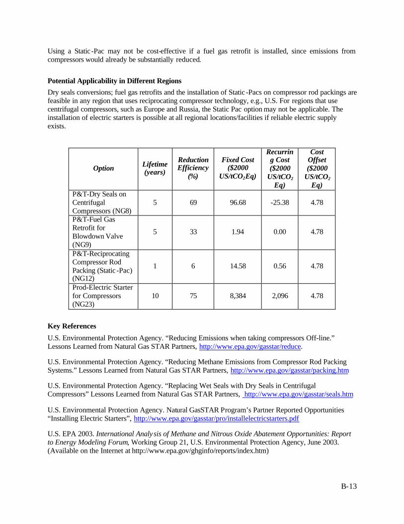
B-13

Using a Static -Pac may not be cost-effective if a fuel gas retrofit is installed, since emissions from compressors would already be substantially reduced.


Dry seals conversions; fuel gas retrofits and the installation of Static -Pacs on compressor rod packings are feasible in any region that uses reciprocating compressor technology, e.g., U.S. For regions that use centrifugal compressors, such as Europe and Russia, the Static Pac option may not be applicable. The installation of electric starters is possible at all regional locations/facilities if reliable electric supply exists.



(%)

Fixed Cost ($2000

US/tCO2Eq)

Recurring Cost ($2000

US/tCO2

Eq)

Cost Offset ($2000

US/tCO2

Eq) P&T-Dry Seals on Centrifugal Compressors (NG8)

5 69 96.68 -25.38 4.78

P&T-Fuel Gas Retrofit for Blowdown Valve (NG9)

5 33 1.94 0.00 4.78

P&T-Reciprocating Compressor Rod Packing (Static -Pac) (NG12)

1 6 14.58 0.56 4.78

Prod-Electric Starter for Compressors (NG23)

10 75 8,384 2,096 4.78

Key References

U.S. Environmental Protection Agency. “Reducing Emissions when taking compressors Off-line.” Lessons Learned from Natural Gas STAR Partners, http://www.epa.gov/gasstar/reduce.

U.S. Environmental Protection Agency. “Reducing Methane Emissions from Compressor Rod Packing Systems.” Lessons Learned from Natural Gas STAR Partners, http://www.epa.gov/gasstar/packing.htm

U.S. Environmental Protection Agency. “Replacing Wet Seals with Dry Seals in Centrifugal Compressors” Lessons Learned from Natural Gas STAR Partners, http://www.epa.gov/gasstar/seals.htm

U.S. Environmental Protection Agency. Natural GasSTAR Program’s Partner Reported Opportunities “Installing Electric Starters”, http://www.epa.gov/gasstar/pro/installelectricstarters.pdf


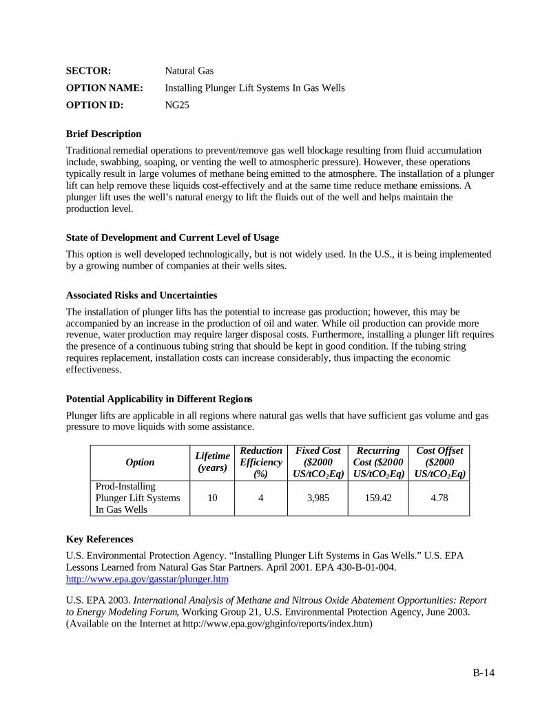
B-14

SECTOR: Natural Gas

OPTION NAME: Installing Plunger Lift Systems In Gas Wells

OPTION ID: NG25

Brief Description

Traditional remedial operations to prevent/remove gas well blockage resulting from fluid accumulation include, swabbing, soaping, or venting the well to atmospheric pressure). However, these operations typically result in large volumes of methane being emitted to the atmosphere. The installation of a plunger lift can help remove these liquids cost-effectively and at the same time reduce methane emissions. A plunger lift uses the well’s natural energy to lift the fluids out of the well and helps maintain the production level.


This option is well developed technologically, but is not widely used. In the U.S., it is being implemented by a growing number of companies at their wells sites.


The installation of plunger lifts has the potential to increase gas production; however, this may be accompanied by an increase in the production of oil and water. While oil production can provide more revenue, water production may require larger disposal costs. Furthermore, installing a plunger lift requires the presence of a continuous tubing string that should be kept in good condition. If the tubing string requires replacement, installation costs can increase considerably, thus impacting the economic effectiveness.


Plunger lifts are applicable in all regions where natural gas wells that have sufficient gas volume and gas pressure to move liquids with some assistance.



(%)

Fixed Cost ($2000

US/tCO2Eq)


Cost Offset ($2000

US/tCO2Eq) Prod-Installing Plunger Lift Systems In Gas Wells

10 4 3,985 159.42 4.78

Key References

U.S. Environmental Protection Agency. “Installing Plunger Lift Systems in Gas Wells.” U.S. EPA Lessons Learned from Natural Gas Star Partners. April 2001. EPA 430-B-01-004. http://www.epa.gov/gasstar/plunger.htm


B-15

SECTOR: Natural Gas

OPTION NAME: Catalytic Converter

OPTION ID: NG2

Brief Description

A catalytic converter burns the emitted methane from incomplete fuel combustion, thus reducing emissions of natural gas into the atmosphere.


This option is well developed technologically. Other than possibly developed regions, such as Europe and U.S., which have emission control requirements, the current level of usage for this option is not widespread.


None.


This option is applicable to all regions.



(%)

Fixed Cost ($2000

US/tCO2Eq)


Cost Offset ($2000

US/tCO2Eq) P&T - Catalytic Converter 10 56 91.46 4.82 0.00

Key References


B-16

SECTOR: Natural Gas

OPTION NAME: Use of Gas Turbines Instead of Gas Reciprocating Engines.

OPTION ID: NG17

Brief Description

Turbines have a better combustion efficiency compared to reciprocating engines; consequently, replacing reciprocating engines with turbines reduces methane emissions.


Turbines are well developed technologically, and are currently widely implemented in several regions, including the OECD-Europe, Eastern and Central Europe, and FSU regions.


Natural gas turbines typically require a constant fuel source; consequently, the use of residual gases from other natural gas processes as an energy supply may not be utilized. Furthermore, if the combustion efficiency of the turbine is lower than the reciprocating engine that it replaces, it is possible that the subsequent increased carbon dioxide emissions will negate the potential methane reductions (EC, 2001).


This option can be implemented in all regions, except those that predominantly utilize turbine compressors, such as the OECD-Europe, Eastern and Central Europe, and FSU regions.



(%)

Fixed Cost ($2000

US/tCO2Eq)


Cost Offset ($2000

US/tCO2Eq) P&T- Use of Gas Turbines Instead of Gas Reciprocating Engines

20 90 152.04 7.60 0.00

Key References


B-17

SECTOR: Natural Gas

OPTION NAME: Altering Start-up Procedures During Maintenance

OPTION ID: NG1

Brief Description

During monthly “cleaning” maintenance, turbines are typically shut down and operations switched to another unit. To reduce the emissions associated with depressurizing the compressor, the turbines can be cleaned while on-line (running). This procedure reduces the number of compressor depressurizations required per year. State of Development and Current Level of Usage

The option is well developed technologically, and is utilized by other industries for cleaning natural gas turbines (EC, 2001); however, it is not widely implemented in the natural gas industry. Associated Risks and Uncertainties

The proposed option involves the spraying of deionised water into the compressor while online (running) (EC, 2001). Since this method is utilized in various other industries, there is little risk or uncertainty associated with this application.


This option can be implemented in all regions that utilize natural gas centrifugal compressors.

Key References




(%)

Fixed Cost ($2000

US/tCO2Eq)


Cost Offset ($2000

US/tCO2Eq) P&T-Altering Start-Up Procedure during Maintenance

1 100 0.00 0.00 4.78

B-18

SECTOR: Natural Gas

OPTION NAME: Replacement of Cast Iron/Unprotected Steel Pipeline/Replacement of Unprotected Steel Services.

OPTION ID: NG34, NG35

Brief Description

Cast iron and unprotected steel pipeline link the natural gas distribution system and are prone to corrosion and leaks. They should be replaced with pipeline made of non-corrosive material that will reduce methane losses from the distribution system. Plastic or protected steel pipelines are good replacements.

Unprotected steel services are low pressure lines that link the distribution system to the consumer and are similarly prone to corrosion and leaks. They should be replaced with services made of non-corrosive material, such as plastic or protected services, which will reduce methane losses from the distribution system.


These options are well developed technologically, and are widely implemented in several regions, including the U.S. and Europe. Associated Risks and Uncertainties

Replacing pipelines and services will involve high capital costs and extensive digging, which may be inconvenient in populated areas.


This option can be implemented in all regions.



(%)

Fixed Cost ($2000

US/tCO2Eq)


Cost Offset ($2000

US/tCO2Eq) D-Replace Cast Iron/Unprotected Steel Pipeline (NG34)

5 95 17,259 0.86 4.78

D-Replace Unprotected Steel Services (NG35)

5 95 410,827 82.17 4.78

Key References


B-19

SECTOR: Natural Gas

OPTION NAME: Electronic Monitoring at Large Surface Facilities

OPTION ID: NG33

Brief Description

Natural gas distribution systems supply gas to meet nearby customer demand. Since peak demand periods are infrequent, distribution systems operate at high gas pressures to ensure that peak and non-peak operating pressures are met. High system operating pressures contribute to higher operating costs and increased gas leakage. By installing electronic monitoring systems, the distribution system pressure can match real time demand more closely and thus reduce fugitive methane emissions.


This option is well developed technologically. It is used in the US and Europe. However, due to cost and infrastructural requirements the level of usage in developing regions is low.


Currently, there are several electronic monitoring methods available, each with varying costs and effectiveness based on the type of distribution system being upgraded. For example, for older systems using cast iron piping, which leak more, the potential savings from reduced gas loss and leak repair costs may justify the cost of more accurate automated control systems.


This technology is applicable in all regions. However, since the hardware required for electronic monitoring includes connections to electrical power supply, the implementation will be subject to infrastructural requirements. For developing regions such as China and Africa, their electricity consumption is estimated to grow at a rate of 4.2 percent annually through 2020; consequently, this growth will result in significant expansion of their local infrastructures (EIA, 2002).



(%)

Fixed Cost ($2000

US/tCO2Eq)


Cost Offset ($2000

US/tCO2Eq) D-Electronic Monitoring at Large Surface Facilities

5 95 28.07 4.68 4.78

Key References

Energy Information Administration, March 2002, “International Energy Outlook, 2002.” DOE/EIA-0484 (2002).


B-20

SECTOR: Natural Gas

OPTION NAME: Portable Evacuation Compressor for Pipeline Venting


Brief Description

To conduct pipeline repairs and maintenance under safe working conditions requires that pipelines are “blown down” (i.e., depressurized) to atmosphere to remove any gas present. This option relates to the use of portable compressors to lower gas line pressure by up to 90 percent of its original value without venting.


This option is well developed technologically, and is currently used in several regions, including the U.S. and Europe. For other regions, such as Eastern Europe and Russia, usage levels for this option may be low, due to a lack of sector investment.


Using a portable compressor is only possible if the compressor can physically connect to the pipeline. Consequently, portable compressors require the presence of a downstream block valve that separates the pressurized and non-pressurized sides of the pipeline. Furthermore, the use of these compressors is generally only appropriate for situations where there is planned maintenance. During an emergency when the pipeline requires immediate depressurization, mobilizing the compressor may be a problem.


Technologically, portable compressors can be used on any pipeline. However, the primary infrastructural condition for use of the compressor is whether the pipeline has sufficient manifolding to enable the compressor to connect to it. It is assumed that this infrastructural condition is present for all regions, and that potential applicability is not affected.



(%)

Fixed Cost ($2000

US/tCO2Eq)


Cost Offset ($2000

US/tCO2Eq) P&T-Portable Evacuation Compressor for Pipeline Venting (NG11)

15 72 318.58 2.28 4.78

Prod-Portable Evacuation Compressor for Pipeline Venting (NG26)

15 72 318.58 2.28 4.78

B-21

Key References

U.S. Environmental Protection Agency. “Using Pipeline Pump-Down Techniques to Lower Gas Line Pressure Before Maintenance.” Lessons Learned from Natural Gas STAR Partners, http://www.epa.gov/gasstar/usepipepump.htm


B-22

SECTOR: Natural Gas

OPTION NAME: Directed Inspection and Maintenance (DI&M)

OPTION ID: NG3 to NG7, NG18 to NG22, NG31, and NG32

Brief Description

Directed inspection and maintenance programs involve surveying facilities and equipment to identify sources of leak. This information can be used to direct maintenance activities to make cost-effective repairs. Enhanced DI&M is a more aggressive DI&M program that involves increased survey and repair frequencies. It costs more but also achieves greater gas savings.


This option is well developed technologically, and is widely used in several regions, including the U.S. and Europe. For other regions, such as Russia, where there is a low level of sector investment, DI&M may not occur to the levels experienced in the U.S. or Europe.


None.


All instrumentation used for screening and measurement is available to all regions.



(%)

Fixed Cost ($2000

US/tCO2Eq)


Cost Offset ($2000

US/tCO2Eq) P&T-D I&M (Compressor Stations) (NG3)

5 13 0.57 1.86 4.78

P&T-D I&M (Compressor Stations: Enhanced) (NG4)

5 20 0.40 2.43 4.78

P&T-D I&M (Enhanced: Storage Wells) (NG5)

5 50 38.11 50.82 4.78

P&T-D I&M (Pipeline: Transmission) (NG6)

5 60 786.60 1,179.90 4.78

P&T-D I&M (Wells: Storage) (NG7)

5 33 38.50 38.50 4.78

Prod-D I&M (Chemical 5 40 123.15 6.82 4.78

B-23

Inspection Pumps) (NG18) Prod-D I&M (Enhanced) (NG19)

5 50 246.40 344.96 4.78

Prod-D I&M (Offshore) (NG20)

5 33 45.82 15.27 4.78

Prod-D I&M (Onshore) (NG21) 5 33 193.25 289.88 4.78

Prod-D I&M (Pipeline Leaks) (NG22)

5 60 22.78 34.18 4.78

D-D I&M (Distribution) (NG31)

5 26 4.88 5.76 4.78

D-D I&M (Enhanced: Distribution) (NG32)

5 66 21.14 21.09 4.78

Key References

U.S. Environmental Protection Agency. 1997. “Directed Inspection and Maintenance at Compressor Stations”. U.S. EPA Lessons Learned from Natural Gas Star Partners. October 1997. EPA 430-B-97-009. http://www.epa.gov/gasstar/direct.htm.


B-24

SECTOR: Natural Gas

OPTION NAME: Reducing the Glycol Circulation Rates in Dehydrators/Installation of Flash Tank Separators


Brief Description

Reducing glycol circulation rates in dehydrators: Tri-ethylene Glycol (TEG) is used in dehydrators to absorb water from gas before it enters the pipeline. During this process, however, TEG also absorbs some methane, which is then vented to the atmosphere when the glycol is regenerated. The amount of methane absorbed is directly proportional to the TEG circulation rate. Maintaining the glycol circulation rate at an optimal level will ensure that methane emissions are kept at a minimum. Installation of flash tank separators: A flash tank separator operates by ‘flashing’ (or vaporizing) methane that is absorbed in TEG. This is achieved by reducing the pressure of the TEG stream in the dehydrator. The flashed methane can be collected for sale or use as a fuel gas.


This option is well developed technologically; however it is not widely implemented. For example, in the U.S., most dehydrators do not have flash tank separators, and vent all of the methane to the atmosphere. In the U.S., flash tanks are typically not used on dehydration units that process less than one million cubic feet (MMCF) of gas per day. For units processing more than one but less than five MMCF/day, approximately 60 percent utilize flash tanks, while for those that process more than five MMCF/day, approximately 30 percent operate with flash tanks.


The costs to install flash tank separators are dependent on several facility-specific conditions such as, the location, terrain, automation and instrumentation. Depending on these site-specific factors, installation costs may increase by over 80 percent, which would impact the economic attractiveness of the option, particularly in undeveloped regions.

B-25


The implementation of flash tank separators and the reduction of glycol dehydration rates are applicable to all regions.



(%)

Fixed Cost ($2000

US/tCO2Eq)


Cost Offset ($2000

US/tCO2Eq) P&T-Installation of Flash Tank Separators (Transmission & Storage) (NG10)

5 61 32.59 0.00 4.78

P&T- Reducing the Glycol Circulation Rates in Dehydrators (not applicable to Kimray pumps) (NG13)

1 30 0.00 0.87 4.78

Prod-Installation of Flash Tank Separators (Production) (NG24)

5 54 100.98 0.00 4.78

Prod-Reducing the Glycol Circulation Rates in Dehydrators (not applicable to Kimray pumps) (NG27)

1 31 0.00 1.72 4.78

Key References


U.S. Environmental Protection Agency. “Reducing the Glycol Circulation Rates in Dehydrators.” Lessons Learned from Natural Gas STAR Program, U.S. Environmental Protection Agency. http://www.epa.gov/gasstar/convertgas.htm

U.S. Environmental Protection Agency. “Installation of Flash Tank Separators.” Lessons Learned from Natural Gas STAR Program, U.S. Environmental Protection Agency. http://www.epa.gov/gasstar/convertgas.htm

B-26

SECTOR: Natural Gas

OPTION NAME: Replacement of high-bleed pneumatic devices with low-bleed pneumatic devices or with Compressed Air Systems.


Brief Description

Natural gas-powered pneumatic devices are widely used for process control applications like pressure, temperature, liquid level and flow-rate regulation. These pneumatic devices are designed to emit natural gas as part of their normal operations, which depending on the type of device/operation can be quite large. Such high-bleed pneumatic devices can be replaced with low-bleed devices that are designed to emit about 80-90% less methane. Another option is to replace the high-bleed devices with compressed air systems. This option will completely eliminate the methane emissions from these pneumatic devices.


These options are well developed technologically, and are implemented in many countries, including the U.S. and Canada. In other regions, such as Europe, natural gas operated devices are not common, since most pneumatics are controlled by electricity or pressurized air. Consequently, emissions from pneumatics in Europe are negligible.


Compressed air systems require electric power and an air compressor to operate. Therefore a reliable power supply and compressor are required to ensure consistent operation of the air system.


Facilities that are situated in remote locations may not have existing power supplies. In such locations, the cost of installing a power generating facility may not be economical. Therefore, installations of compressed air systems are more suitable for facilities that have existing power supply arrangements. Consequently, regions where there is limited electrical infrastructure, such as China and Russia, may have limited applicability. Furthermore, regions, such as Europe, that do not utilize natural gas operated pneumatics may not require this option.

B-27



(%)

Fixed Cost ($2000

US/tCO2Eq)


Cost Offset ($2000

US/tCO2Eq) P&T-Replace High-bleed pneumatic devices with compressed air systems (NG14)

5 100 7.09 64.48 4.78

P&T-Replace high-bleed pneumatic devices with low-bleed pneumatic devices (NG15)

5 86 14.01 0.00 4.78

Prod-Replace High-bleed pneumatic devices with compressed air systems (NG28)

5 100 6.82 62.06 4.78

Prod-Replace high-bleed pneumatic devices with low-bleed pneumatic devices (NG29)

5 86 14.01 0.00 4.78

Key References


U.S. Environmental Protection Agency. “Convert Gas Pneumatic Controls to Instrument Air”. Lessons Learned from Natural Gas STAR Program, U.S. Environmental Protection Agency. http://www.epa.gov/gasstar/convertgas.htm

U.S. Environmental Protection Agency. “Options for Reducing Methane Emissions from Pneumatic Devices in the Natural Gas Industry”. Lessons Learned from Natural Gas STAR Program, U.S. Environmental Protection Agency. http://www.epa.gov/gasstar/pneumat.htm

B-28

SECTOR: Natural Gas

OPTION NAME: Surge Vessels for Station/Well Venting


Brief Description

A large quantity of methane is vented as a result of well blowdowns or station venting. Surge vessels enable the capture of methane, thus avoiding venting, for rerouting to pipelines or fuel use.


This option is well developed technologically, but is not widely used, due to high capital costs.


Implementing surge vessels at compressor stations and well sites will involve high capital costs and extensive digging, which may have safety implications.





(%)

Fixed Cost ($2000

US/tCO2Eq)


Cost Offset ($2000

US/tCO2Eq) P&T-Surge Vessels for Station/Well Venting (NG16)

10 50 11,226 224.52 4.78

Prod-Surge Vessels for Station/Well Venting (NG30)

10 50 11,226 224.52 4.78

Key References


B-29

SECTOR: Landfills of Solid Waste

OPTION NAME: Anaerobic digestion 1, Anaerobic digestion 2

OPTION ID: LF1, LF2

Brief Description

In landfills, the decomposition of organic material without oxygen occurs naturally. Anaerobic digestion expedites this process by using a vessel that excludes oxygen and maintains the temperature, moisture content and pH close to their optimum values. Methane from anaerobic digestion plants can be used to produce heat and/or electricity. The solid residue from the process can be ‘cured’ under aerobic conditions to form a substance that can be used as a soil improver, which has a market value. Costs include the plant investment and operating costs, as well as the landfill disposal of low quality residues. Income from compost, income from energy, and avoided landfilling are treated as negative costs.

Two variants of anaerobic digestion option were analyzed in the EC report (EC, 2001). One of them, with lower costs and higher benefits, did not include the cost of source separating the waste prior to disposal in the anaerobic digestion system (AD1). The other option incorporated this cost (AD2).


Anaerobic digestion is a well-developed technology and is widely used in EU countries . In some of the FSU countries (e.g., Russia and Ukraine) this technology is tested at pilot facilities.


Anaerobic digestion is economically feasible if sufficient quantities of methane gas and high-quality residue are produced to offset the project costs, and if a market exists for this methane and residue. Anaerobic digestion requires a well-controlled environment. Consequently, if the environment is not properly controlled, methane recovery may be insufficient to support the project costs. Similarly, to the extent that contamination occurs, the value of the solid residue can be significantly diminished.


Technologically, anaerobic digestion can be applied in any location with sufficient market for energy produced by anaerobic digestion plants If the methane from an anaerobic digestion facility is directly combusted (e.g., in an industrial boiler), the technology requires an energy end user and adequate pipeline infrastructure.



(%)

Fixed Cost ($2000

US/tCO2Eq)


Cost Offset ($2000

US/tCO2Eq) Anaerobic Digestion 1 15 95 400.98 67.61 8.74 Anaerobic Digestion 2 15 95 484.91 125.89 5.25

Key References


B-30


OPTION NAME: Composting (1 and 2), Mechanical Biological Treatment

OPTION ID: LF3 to LF5

Brief Description

Both composting and mechanical biological treatment involve degradation of the organic matter under aerobic conditions. Composting can be done in private households (home composting) and in central locations. If done in a central location, a number of methods are available, including windrow systems and tunnel composting. In both households and central locations, composting requires separating organic matter from the waste stream. Finished compost has a market value, as it can be used to enhance soil in horticulture/landscape and agricultural sites.

Mechanical-biological treatment (MBT) does not involve separating out the organic matter. Rather, the whole waste stream is composted in order to aerobically degrade the organic fraction. However, while the technology eliminates the need for source separation, the inorganic matter that does not degrade becomes residue that must be disposed of in a landfill. The process also does not create a useable by-product. EC study analyses two variants of the composting option (CM1 and CM2) : the first composting option is a 25,000 ton/year tunnel plant, based on an existing plant in the UK; the second option is a 50,000 ton/yr tunnel plant, based on an existing plant in the Netherlands.


Composting is a well-developed technology that is currently applied in many regions, and is being heavily promoted in several EU countries. Implementation of mechanical biological treatment is much less common, and the technology is currently applied in only a few regions globally.


Both options become economically feasible if source separation costs are minimal. In addition, the composting process must be well managed in an aerobic environment, as methane formation may otherwise occur. Finally, the potential market value of compost is likely to fluctuate by region and over time.


Technologically, both composting and mechanical biological treatment can be applied in any region of the world



(%)

Fixed Cost ($2000

US/tCO2Eq)


Cost Offset ($2000

US/tCO2Eq) Composting 1 15 100 359.02 93.25 0.00 Composting 2 15 100 424.29 81.59 0.00 Mechanical Biological Treatment 15 95 359.02 121.23 0.00

B-31

Key References


B-32


OPTION NAME: Heat Production

OPTION ID: LF6

Brief Description

Landfill gas is piped directly to a nearby end user to be used as a replacement or supplementary fuel source. Examples of end uses include industrial boilers, brick kilns and lime or cement kilns. In these projects, the sale of recovered gas becomes a cost offset.


Heat production from landfill gas is a well-developed technology that is commonly applied in North America and European Union.


Heat production projects require a sufficient demand for landfill gas such that market prices for the gas can support the project. In addition, the landfill must produce adequate levels of methane in order to generate enough revenue to offset project costs. Finally, landfills must be located near the end consumer in order to minimize pipeline costs.


Heat production can be applied in countries with landfills that produce significant quantities of methane to offset project costs, and in which there is significant market demand for landfill gas as a heat source. The technology may not be available in unmanaged landfills, since these landfills typically lack the anaerobic conditions necessary for significant levels of methane formation.



(%)

Fixed Cost ($2000

US/tCO2Eq)


Cost Offset ($2000

US/tCO2Eq) Heat Production 20 70 7.30 1.71 6.03

Key References


B-33


OPTION NAME: Increased Oxidation

OPTION ID: LF7

Brief Description

Improving the capping and restoration layers reduces methane emissions. A clay cap minimizes methane leakage, while landfill cover soils above the cap oxidize escaping methane. Costs include installing the clay cap and restoration layer, and annual maintenance costs.


Capping and covering is already a common practice in countries with modern landfills.


Costs are highly dependent on the availability of clay for improving the cap and soil for improving the cover. Costs will increase significantly if these materials must be transported from far distances.


Increasing oxidation (IO) of landfill gas is applicable to countries with managed landfills that produce methane. The technology is not applicable to countries in which waste is deposited in unmanaged landfills, since these landfills already operate in an aerobic environment, and consequently produce little methane.



(%)

Fixed Cost ($2000

US/tCO2Eq)


Cost Offset ($2000

US/tCO2Eq) Increased Oxidation 50 44 465.43 0.63 0.00

Key References


B-34


OPTION NAME: Direct Gas Use – Profitable at Base Price, Direct Gas Use – Profitable above Base Price

OPTION ID: LF8, LF9

Brief Description

Landfill gas is piped directly to a nearby end user for use as a replacement of natural gas In these projects, the sale of the landfill gas offsets the costs for the project. Costs include a gas collection and flare system, gas treatment, gas compression to 50 pounds per square inch (psi), and a five-mile gas pipeline to a customer. Two variants of this option are analyzed: direct gas use is profitable at a base energy price of $2.74/mmBtu (DG1) and direct gas use profitable above this base price (DG2). The cost and potential reductions for both of these options were estimated as a function of landfill size (using a model of U.S. landfills). Larger landfills, in which sufficient methane was generated to offset project costs, were more likely to be profitable under the base price than smaller landfills.


Direct gas use projects are well developed and account for approximately one third of U.S. landfill gas-to-energy projects.

Associated Risks and Uncertaintie s

Direct gas projects require a sufficient demand for landfill gas such that market prices for the gas can support the project. In addition, the landfill must produce adequate levels of methane in order to generate enough revenue to offset project costs. Finally, landfills must be located near the end consumer in order to minimize pipeline costs.


Direct gas projects can be applied in countries with landfills that produce significant quantities of methane to offset project costs, and in which the end user is in relatively close proximity to the landfill. The technology is not applicable to countries in which waste is deposited in unmanaged landfills, since these landfills typically lack the anaerobic conditions necessary for significant levels of methane formation.



(%)

Fixed Cost ($2000

US/tCO2Eq)


Cost Offset ($2000

US/tCO2Eq) Direct Gas Use (profitable at base price)

15 75 36.20 2.84 4.78

Direct Gas Use (profitable above base price)

15 75 44.72 3.50 4.78

B-35

Key References

US EPA. 1999. U.S. Methane Emissions 1990-2010: Inventories, Projections, and Opportunities for Reductions. Office of Air and Radiation, U.S. Environmental Protection Agency, Washington, D.C.


B-36


OPTION NAME: Electricity Generation

OPTION ID: LF10

Brief Description

Recovered methane is used to power a generating set and a connection is established to the electricity distribution network. Costs include capital and O&M associated with the collection system, flare system, and electricity production system. The analysis assumes electricity is produced using a reciprocating internal combustion (IC) engine. Income from energy sales is included as a negative cost.


Electricity generation (EG) is a well-developed technology that is applied in the United States, European Union, FSU, and some developing countries (e.g., India).


Electricity generation is feasible if sufficient electricity is generated to offset project costs. This condition requires that landfills be sufficiently large so that they generate substantial quantities of methane. In addition, the cost effectiveness of electricity projects largely depends on the market for electricity. Adequate electricity price for sold electricity is a condition for cost-effective projects.


Landfill gas to electricity projects can be applied in countries with landfills that produce enough electricity to offset project costs, and in which the market price for electricity is sufficiently high. The technology is not applicable to countries in which waste is deposited in unmanaged landfills, since these landfills typically lack the anaerobic conditions necessary for significant levels of methane formation.



(%)

Fixed Cost ($2000

US/tCO2Eq)


Cost Offset ($2000

US/tCO2Eq) Electricity Generation 20 75 149.98 8.92 5.96

Key References



B-37


OPTION NAME: Flaring

OPTION ID: LF11

Brief Description

Recovered landfill gas is flared to control odor and gas migration. Costs include the capital and O&M for the recovery and flaring equipment. Costs are based on the peak gas flow rate during the anticipated operating lifetime of the collection system.


Flaring is a well-developed technology that is applied in many regions, including the United States and European Union.


The cost of flaring equipment depends on individual landfill characteristics and gas recovery capacities. Consequently, the cost effectiveness of flaring as a mitigation technology will fluctuate based on these factors.


Flaring can be applied in countries with managed landfills that produce sufficient quantities of methane such that flaring technologies are cost effective. Since developing countries typically have unmanaged landfills with little methane production, flaring has limited applicability in these countries.



(%)

Fixed Cost ($2000

US/tCO2Eq)


Cost Offset ($2000

US/tCO2Eq) Flaring 20 75 26.67 3.91 0.00

Key Refe rences



B-38

SECTOR: Wastewater Management

OPTION NAME: Electricity Generation from Recovered Methane

OPTION ID: W1

Brief Description

Anaerobic processes at wastewater treatment facilities present potential for capture and reuse of methane emissions resulting from digester reactions (biogas). Biogas is typically utilized to generate heat or electricity for reuse by the facility or is sold commercially to a local power company. Technologies such as internal combustion engines, gas turbines, and fuel cells are often employed on-site in order to convert biogas into desired end products. State of Development and Current Level of Usage

In the U.S., methane abatement systems in anaerobic wastewater treatment making their way into conventional use as means to supplement on-site power generation, and even to generate power for purchase by local electric utilities. However, the overall frequency using this technology in industrial and municipal wastewater treatment can be characterized as marginal at best. Comprehensive documentation and sources of aggregate data on a national scale for these implementations are sparse and primarily anecdotal. Industrial sources of interest are considerably more unclear, as treatment methods are often not documented for public knowledge and effluent often contributes to municipal wastewater streams. ICF developed a deterministic approach to estimate abatement quantities and costs based on national estimates for municipal wastewater treatment that incorporates parameters derived from applicable technology evaluations and frequency of use. While some of the parameters used in this analysis are open for discussion (and in some cases are a result of industry-average “best guesses”), the developed approach provides credible approximation of quantities and costs for this option.


This option is normally implemented when it is determined to be economically desirable in an engineering cost-benefit study. The degree of return on investment normally justifies pursuit of biogas reuse, however, it depends on regional energy prices. Variability in a facility’s annual operating conditions and parameters is generally minimal.


Biogas reutilization is technically applicable wherever anaerobic digestion has been implemented. Anaerobic digestion is more prominent in areas with a high density of environmentally sensitive receptors, where real estate is tight, and odour control is a major requirement. Regions with higher urban density are more likely candidates for such processes, as opposed to lagoons or aerobic processes. Approach to Developing Technological and Cost Characteristics of the Wastewater Management Option Personal communication with an industrial manufacturer1 of anaerobic digesters indicates that approximately 70% of all air emissions from wastewater treatment are actually captured by an anaerobic digester installation.

1 Framatome ANP DE&S (formerly Duke Engineering & Services)

B-39

The fixed costs for the anaerobic digestion option were estimated based on the U.S. circumstances. The total amount of (captured) methane emissions originating from anaerobic digestion, which represents the total potential available nationally for abatement and reuse under this option, is estimated to be more than 909 kilotonnes of CH4 in 2000. Based on methane LHV and assuming 50 percent average combustion efficiency in electrical conversion equipment (including turbines, internal combustion engines, fuel cells, and combinations thereof), a magnitude of approximately 4.2 billion kilowatt-hours (kWh) is a total amount of electricity that can be generated by this option in the U.S. In estimating the costs associated with the electricity generation option, it is imperative to separate the costs of construction and maintenance of the anaerobic digester from the methane collection and generation equipment. The costs associated with this option only reflect the collection and generation , and exclude the costs of constructing and operating the entire anaerobic system. Cogeneration costs from a few sites in North America, which implement methane abatement and reuse technologies, were compiled to generate a crude linear regression with plant capacity as the independent variable [(r2) = 0.72]. Costs were inflated to reflect $ (2000) U.S. The regression was applied to the total wastewater capacity available to this option and resulted in a unit capital cost of $262/tonne CH4. Recurring costs were estimated using an engineering estimate of 5 percent of capital costs2, or about $13/tonne CH4. The cost offset for the electricity generation option was set at the same level as for the option of using landfill gas for electricity generation.



(%)

Fixed Cost ($2000

US/tCO2Eq)


Cost Offset ($2000

US/tCO2Eq) Electricity Generation from Recovered Methane

30 70 11.39 0.57 5.96

Key References

Buckius, Howell. (1992) Fundamentals of Engineering Thermodynamics. New York: McGraw-Hill, Inc., p. 730

Intergovernmental Panel on Climate Change, Greenhouse Gas Inventory Reference Manual: Revised 1996 IPCC Guidelines for National Greenhouse Gas Inventories, Vol. 3 (Paris, France, 1997)

Energy Information Administration, Form EIA-861, "Annual Electric Utility Report", 2000.

Framatome ANP DE&S (formerly Duke Engineering & Services)

2 Dr. Kannan Vembu, P.E., pers. comm..

B-40

SECTOR: Nitric Acid Production

OPTION NAME: BASF - High Temperature Catalytic Reduction Method (BASF – HTCR)

OPTION ID: NAC1

Brief Description

This is a high temperature catalytic reduction method proposed by BASF that decomposes N2O to nitrogen (N2) and oxygen (O2) by using a catalyst. The catalyst composition is 'O3-80' : CuO on an Al2O3 carrier. The catalyst is used directly behind the Pt/Rh gauzes in the ammonia burner. The catalyst decomposes the N2O gas at high temperatures (800 °C to 900 °C) to nitrogen (N2) and oxygen (O2).


The catalyst has been installed and is currently being tested inside a commercially operating plant.


There is an uncertainty to the claim by BASF that the catalyst leads to no NO conversion with a 0.3 to 0.5% error after being more than 2 years operational in 2 commercial scale plants. Possible safety problems exist with Cu occurrence in the fertilizer product; sometimes a filter is needed.


The design of the BASF catalyst bed can be implemented in any standard HNO3 plant.



(%)

Fixed Cost ($2000

US/tCO2Eq)


Cost Offset ($2000

US/tCO2Eq) BASF-HTCR 10 80 2.76 0.17 0.00

Key References

Jos Kuiper. 2001. “High Temperature Catalytic Reduction of Nitrous Oxide Emission from Nitric Acid Production Plants.” Continental Engineering, No. 1, Amsterdam, The Netherlands, October 2001. NOVEM Project No. 375001/0080.

B-41


OPTION NAME: ECN - Low temperature selective catalytic reduction with propane addition (ECN – LTSCR)

OPTION ID: NAC2

Brief Description

ECN uses an extra reactor to convert the N2O in the off-gas of the production process. Propane is used as an additive in this reduction process. Propane is mixed with the off-gas stream before entering the reactor. The product stream of the production process is not influenced because this method reduces the N2O in the off-gas of the production process. The catalyst composition is a Fe-NH4-Zeolite-27 or 55-type catalyst.


This option is in the lab test phase. A pilot plant scale test has been considered. Associated Risks and Uncertainties

Only lab tests have been done, consequently, information is not available yet on the associated risks and uncertainties.


This option can be potentially applied at any nitric acid production facility.



(%)

Fixed Cost ($2000

US/tCO2Eq)


Cost Offset ($2000

US/tCO2Eq) ECN-LTSCR 10 95 3.64 1.81 0.00

Key References


B-42


OPTION NAME: Grand Paroisse - High Temperature Catalytic Reduction Method (Grand Paroisse – HTCR)

OPTION ID: NAC3

Brief Description

The abatement method developed by Grande Paroisse uses the high temperature reduction catalyst to convert N2O into NO, resulting in higher HNO3 production. This process has only been proven in laboratory scale tests. The catalyst composition is aluminum oxide and zirconium oxide. State of Development and Current Level of Usage

This option is in the laboratory test phase.


Various laboratory tests have been conducted. Each test lasts 24 hours and the total of 33 tests have been completed. Since this method is in the test phase its risk and uncertainties are still unknown.


The design of the Grand Paroisse catalyst bed can be implemented in any standard HNO3 plant.



(%)

Fixed Cost ($2000

US/tCO2Eq)


Cost Offset ($2000

US/tCO2Eq) Grand Paroisse - HTCR 10 77.6 3.09 0.16 0.00

Key References


B-43


OPTION NAME: HITK – High Temperature Catalytic Reduction Method (HITK – HTCR)

OPTION ID: NAC4

Brief Description

This is a high temperature catalytic reduction technology by HITK (Hermsdorfer Institut für Technische Kerami) that decomposes N2O to nitrogen (N2) and oxygen (O2) by using a catalyst. The catalyst composition is metal oxide preferably La, Cr, Mn, Fe, Co, Ni and Cu. The catalyst is used directly behind the Pt/Rh gauzes in the ammonia burner. The catalyst decomposes the N2O gas at high temperatures (800 °C to 900 °C) to nitrogen (N2) and oxygen (O2).


Laboratory tests were used for the patent. As of October 2001, final tests on the pilot plant stage were not yet available.


As of October 2001, final tests on the pilot plant stage were not yet available , so the associated risks and uncertainties are unknown.


The bedheight required for the HITK method is 145 mm and may not fit into the standard HNO3 plant. Since no research of regional differences in production technologies were available for this study, the TA was assumed to be equal to 100 percent.



(%)

Fixed Cost ($2000

US/tCO2Eq)


Cost Offset ($2000

US/tCO2Eq) HITK- HTCR 10 100 3.18 0.22 0.00

Key References


B-44


OPTION NAME: Krupp Uhde - Low Temperature Catalytic Reduction Method (Krupp Uhde – LTCR)

OPTION ID: NAC5

Brief Description

The low temperature selective catalytic N2O-reduction method developed by Krupp Uhde uses a zeolite type catalyst. The catalyst bed is installed in the tail-gas stream of a commercially operating plant. All N2O is reduced to N2 and O2. There is an extra reactor needed after the ammonia burner. According to Krupp Uhde, low temperature catalysts have a longer lifetime than the high temperature catalysts.


Development stage is at the pilot plant level.


The catalyst life test is needed.


The method is potentially applicable at all production facilities.



(%)

Fixed Cost ($2000

US/tCO2Eq)


Cost Offset ($2000

US/tCO2Eq) Krupp Uhde - LTCR 10 95 3.45 0.20 0.00

Key References

Jos Kuiper. 2001. “High Temperature Cata lytic Reduction of Nitrous Oxide Emission from Nitric Acid Production Plants.” Continental Engineering, No. 1, Amsterdam, The Netherlands, October 2001. NOVEM Project No. 375001/0080.

B-45


OPTION NAME: Norsk Hydro - High Temperature Catalytic Reduction Method (Norsk Hydro – HTCR)

OPTION ID: NAC6

Brief Description

Norsk Hydro has developed a high temperature catalytic reduction method, which decomposes N2O to nitrogen (N2) and oxygen (O2) by using a catalyst (NH-1 or NH-2). Laboratory tests show 0.2 to 0.4 % NO losses but this is below the detection limit. The catalyst is used directly behind the Pt/Rh gauzes in the ammonia burner. The catalyst decomposes the N2O gas at high temperatures (800 °C to 900 °C) to nitrogen (N2) and oxygen (O2).


The catalyst is installed inside a commercially operating plant. For the NH-2 catalyst pilot plant tests have been done, and the commercial plant scale test was planned for early 2001. As of October 2001 the catalyst had been in operation for 18 months.


This method has no known uncertainties.


The design of the Norsk Hydro catalyst bed can be implemented in any standard HNO3 plant.



(%)

Fixed Cost ($2000

US/tCO2Eq)


Cost Offset ($2000

US/tCO2Eq) Norsk Hydro- HTCR 10 90 2.32 0.15 0.00

Key References


B-46


OPTION NAME: Non-Selective Catalytic Reduction (NSCR)

OPTION ID: NAC7

Brief Description

NSCR uses a fuel and a catalyst to consume free oxygen in the tail gas and to convert NOx to elemental nitrogen. The gas from the NOx abatement is passed through a gas expander for energy recovery. NSCR units produce stack gases in the 1000 to 1100oF range that requires more exotic materials of construction for the expander and higher maintenance costs. Since all oxygen must be consumed before the nitrogen oxides are reduced, excess fuel must be used resulting in methane emissions. NSCR can reduce N2O emissions by 80-90 percent. However, this process requires additional fuel (natural gas) and, as a result of combustion not only CO2 but also carbon monoxide, ammonia, uncombusted hydrocarbons 3 and even small amounts of hydrocyanic acid are emitted. NSCR units are generally not preferred in modern plants because of high operational temperatures.

State of Development and Current Leve l of Usage

NSCRs were widely installed in nitric plants built between 1971 and 1977. NSCR is a typical tail gas treatment in the U.S. and Canada with less application in other parts of the world. It is estimated that approximately 20 percent of nitric acid plants in the U.S. use NSCR.


Process requires additional fuel (natural gas) and, as a result of combustion, CO2 as well as other harmful emissions are produced.


NSCR is potentially applicable in all regions.



(%)

Fixed Cost ($2000

US/tCO2Eq)


Cost Offset ($2000

US/tCO2Eq) NSCR 20 85 6.29 0.16 0.00

Key References

IEA Greenhouse Gas R&D Programme. 2000a. Abatement of Emissions of Other Greenhouse Gases – Nitrous Oxide. International Energy Agency, Cheltenham, UK.

3 Release of additional methane might reduce the GHG abatement effect of this option.

B-47

SECTOR: Adipic Acid Production

OPTION NAME: Valorisation of Nitrous Oxide Emitted by Adipic Acid Unit

OPTION ID: AA1

Brief Description

Valorization is the thermal conversion of N2O into nitrogen and oxygen. During this process NOx is also produced. The aim of this technology is to encourage the production of NOx and minimize the conversion of N2O into nitrogen and oxygen. The NOx formed can be then recycled in the form of nitric acid, which is a raw material in the upstream adipic acid manufacturing process.


A pilot aimed at endorsing the process on an industrial scale was designed and built in Chalampé, France at the beginning of 1996. The first results of this pilot test on site were obtained during the summer of 1996. The design studies of the industrial facility were launched at the end of 1996 and the construction of the plant started very quickly with a very tight schedule. The construction of the plant was finished at the end of 1997 and the start-up of the plant followed in December 1997.


During the first year of operation, this prototype plant operated under harsh temperature conditions and consequently has encountered a certain number of problems of material resistance. These problems required serious maintenance operations to improve the thermal protection of certain sensitive points or certain sensors - mainly the temperature probes. These modifications sometimes led to long downtimes resulting in the plant shutting down for 3 months in the summer of 1998. Another difficulty comes from the fact that this unit treats the process gases from several adipic acid production shops. Therefore, occasionally, it must adapt to the rapid variations in flow or composition of the gases to be treated; otherwise the unit would automatically trigger off a security shut down. Nevertheless, with the advancement of automation, the operation of the plant can adapt to these variations, but the adjustment of the automation system requires a great deal of experience and the operations need monitoring in various conditions.


The valorisation of nitric acid is applicable for an adipic acid facility, which is lacking in nitric acid, because it leads to a reduction in the overall consumption of the nitric acid in the facility.



(%)

Fixed Cost ($2000

US/tCO2Eq)


Cost Offset ($2000

US/tCO2Eq) Valorisation 10 99 N/A N/A N/A

Key References

Klinger, Francois. “Valorisation of nitrous oxide emitted by adipic acid unit.” Control of N2O emissions from various sources. Session 7. Rodhia Alsachime. Chalempe France.

B-48

SECTOR: Adipic Acid Production

OPTION NAME: Thermal Reduction

OPTION ID: AA2

Brief Description

Thermal N2O reduction is the destruction of off-gases in boilers using flame burners with premixed methane (or natural gas). The system eliminates 98 to over 99 percent of N2O and operates from 95 to over 99 percent of the time. This option is currently available and in use. For example in the U.S., 34 percent of production uses thermal destruction.


Four adipic acid plants have thermal reduction technology installed in their facilities.


Cost effectiveness depends on individual plant’s ability to use recovered steam.


This option is potentially applicable in all regions.



(%)

Fixed Cost ($2000

US/tCO2Eq)


Cost Offset ($2000

US/tCO2Eq) Thermal Reduction 20 96 0.38 0.16 0.00

Key References

IEA Greenhouse Gas R&D Programme. 2000a. Abatement of Emissions of Other Greenhouse Gases – Nitrous Oxide. International Energy Agency, Cheltenham, UK.

B-49

SECTOR: Refrigeration and Air-Conditioning

OPTION NAME: Refrigerant Recovery

OPTION ID: R14, R16 and R18

Brief Description

The practice of recovering refrigerant at service or disposal for reuse or destruction can significantly reduce emissions of HFCs. Recovery involves the use of a refrigerant recovery device that transfers refrigerant into a storage container prior to servicing or dispos ing equipment. Once the recovery process is complete, the refrigerant contained in the storage container may be recharged back into the source equipment (for servicing jobs), cleaned through the use of recycling devices, purified for resale at a reclamation facility, or disposed safely through the use environmentally-safe technologies (e.g., incineration) (U.S. EPA, 2001).

Because refrigerant recovery from equipment with large charge sizes is cost effective—given that the refrigerant can be re-used or re-sold—this analysis assumes that such recovery jobs are already practiced in the baseline. As such, this analysis considers only the recovery of refrigerant from small equipment types (i.e., refrigerated transport, domestic refrigerators, and motor vehicle air-conditioning systems [MVACs]), which is less cost-effective due to the smaller recoverable charges. Although the costs of recovery vary by equipment type and recovery scenario (i.e., service and disposal), this analysis looks at the costs of MVAC recovery at service, as this is believed to be the most commonly practiced recovery scenario of those considered.


Refrigerant recovery equipment is widely available and used extensively in developed countries. Indeed, in many developed countries, refrigerant recovery is required by law (e.g., European Union, Canada, United States). In developing countries, however, refrigerant recovery is not widely practiced because of a lack of available capital and infrastructure (e.g., access to recovery/recycling devices reclamation facilities), as well as a lack of national legislation requiring such practice.


Risks and uncertainties associated with recovery are minimal. Proper equipment instructions must be followed so that a minimal amount of refrigerant will escape to the atmosphere during the recovery operation, and to ensure technician safety. There is uncertainty associated with the reduction efficiency of this option, as the amount of refrigerant emissions will depend on technician technique and equipment type. Additionally, there is uncertainty associated with the total percent of emissions from equipment that can be avoided by recovering at service and disposal. This analysis assumes that 50 percent of emissions from small equipment types can be avoided by practicing this option (the remaining 50 percent of emissions from these equipment types is assumed to occur from leakage during operation).


Refrigerant recovery is widely practiced in developed countries in the baseline. It is not, however, assumed to have penetrated a significant portion of the refrigeration and air-conditioning markets in developing countries. Thus, the greatest growth opportunity for this option is in developing countries.

4 “Small appliances” include domestic refrigerators, icemakers, vending machines, dehumidifiers, and water coolers. 5 These scenarios include recovery/recycling of (1) MVACs at service, (2) MVACs at disposal, (3) small appliances at service, and (4) small appliances at disposal.

B-50



(%)

Fixed Cost ($2000

US/tCO2Eq)a

Recurring Cost ($2000 US/tCO2Eq)b

Cost Offset ($2000

US/tCO2Eq)c Recovery—Domestic Refrigeration (R14)

10 95 26.19 3.40 3.05

Recovery—Refrigerated MVACs (R16)

10 95 26.19 3.40 3.05

Recovery—Refrigerated Transport (R18)

10 95 26.19 3.40 3.05

a Based on R-134a MVAC recovery/recycling unit manufactured by Robinair (model #347002K) (Robinair SPX Corporation, 2003).

b Annual cost is based on assumption of 150 recovery jobs/year, each requiring 10 minutes of technician’s time, valued at $14/hr (Jiffy Lube, 2003). c This analysis assumes that 0.55 kg can be recovered per job and that value of refrigerant is $4/kg (Baker 2002; Campbell 2003).

Key References

Baker, James. 2002. Mobile Air Conditioning Sector Update. Presentation at the 19th Meeting of the Ozone Operations Resource Group (OORG), The World Bank, Washington, DC, March 28, 2002.

Campbell, Nick. 2003. Production Sector Update. Presentation at the 20th Meeting of the Ozone Operations Resource Group (OORG), The World Bank, Washington, DC, April 25, 2003.

IEA Greenhouse Gas R&D Programme. 2001. Abatement of Other Greenhouse Gases – Engineered Chemicals. International Energy Agency, Cheltenham, United Kingdom, February 2001. Report Number PH3/35.

Jiffy Lube. 2003. Personal communication with service technician, Jiffy Lube Service Center #273, MD, USA, July 25, 2003.

Robinair SPX Corporation. 2003. Personal communication with sales representative, July 24, 2003.

U.S. EPA (Environmental Protection Agency). 2001. U.S. High GWP Gas Emissions 1990-2010: Inventories, Projections, and Opportunities for Reductions. U.S.EPA #000-F-97-000. Office of Air and Radiation, U.S. Environmental Protection Agency. Washington, DC, June 2001.

B-51


OPTION NAME: Replacing Direct Expansion Systems with Distributed Systems

OPTION ID: R1 and R6

Brief Description

Distributed refrigeration systems are gaining in popularity because they offer the ability to reduce refrigerant charge and eliminate the need for a dedicated mechanical room containing multiple compressor racks. Distributed systems feature multiple smaller units located closer to the refrigerated display cases.

Replacing HFC direct expansion systems with HFC distributed systems in retail food and cold storage applications can reduce HFC emissions. Unlike direct expansion systems with central refrigeration rooms containing multiple compressor racks, distributed systems feature multiple smaller units located closer to the refrigerated display cases, connected by a water loop to a single cooling unit that is located on the roof or outside of the store (U.S. EPA 2001, Copeland 2003). Distributed systems significantly reduce the refrigerant inventory and minimize the length of refrigerant tubing and the number of fittings that are installed in direct expansion systems, thereby reducing leaks of HFCs (Alliance, 1999). In addition, these systems are more energy efficient than direct expansion systems, leading to further reductions in global warming impacts and long-term cost-savings (ORNL BTC, Sand et al., 1997).


Distributed systems are most commonly used in retail food refrigeration and are widely available (U.S. EPA, 2001).


Risks and uncertainties associated with this option are minimal. One risk associated with this option is that, because refrigerant charge is placed throughout the building, the amount of refrigerant charge that could potentially be released into the building is large. Thus, the use of flammable or highly toxic refrigerants is not feasible. In the case of retail food applications, store operators in the U.S. and some other countries will not accept the safety and legal risks, and safety codes prohibit such large quantities of flammable refrigerant to be used in a publicly occupied space (Alliance, 1999).


Distributed systems may be used to replace HFC systems equally across all regions.



(%)

Fixed Cost ($2000

US/tCO2Eq)


Cost Offset ($2000

US/tCO2Eq) Replacing DX with Distributed Systems —Retail Food (R1)

20 100 82.15 -6.84 1.58

Replacing DX with Distributed Systems —Cold Storage (R6)

20 100 82.15 -6.84 1.58

Note: All cost information is from U.S. EPA (2001).

B-52

Key References

Alliance. 1999. Global Comparative Analysis of HFC and Alternative Technologies for Refrigeration, Air Conditioning, Foam, Solvent, Aerosol Propellant, and Fire Protection Applications. Final Report to the Alliance for Responsible Atmospheric Policy. Arthur D. Little, Inc., Cambridge, MA; Reference Number 49648.

Copeland Corporation. 2003. “Emerson Climate Technologies.” Available at http://www.copeland-corp.com/press/2003/2003_26.htm


ORNL BTC (Oak Ridge National Laboratory, Building Technology Center). "Improvements in Commercial Refrigeration," Available online at http://www.ornl.gov/ORNL/BTC/imp-comref.html

Sand, J.R., S.K. Fischer, and V.D. Baxter. 1997. Energy and Global Warming Impacts of HFC Refrigerants and Emerging Technologies. Prepared by Oak Ridge National Laboratory for Alternative Fluorocarbons Environmental Acceptability Study and U.S. Department of Energy. Oak Ridge, TN, pp. 4, 5, 7, 26, 40-42, 58-61, 73-77, 83-85, 122.

U.S.EPA. 2001. U.S. High GWP Gas Emissions 1990-2010: Inventories, Projections, and Opportunities for Reductions. U.S. EPA #000-F-97-000. Office of Air and Radiation, U.S. Environmental Protection Agency. Washington, DC, June 2001.

B-53


OPTION NAME: Ammonia Secondary Loops


Brief Description

Secondary loop systems circulate a secondary coolant or brine from the central refrigeration system to the display cases, thereby operating at reduced charges and achieving isolating lower leak rates (U.S. EPA, 2001). Because these systems isolate customers from the refrigerant, they can use a variety of refrigerants, including ammonia. By using ammonia as the primary refrigerant in secondary loop system in place of HFCs, HFC emissions can be reduced. This technology option is assumed to be appropriate for retail food, cold storage, and industrial process end use sectors (U.S. EPA, 2001).


The use of ammonia is very common in certain countries and strongly restric ted in others (ECOFYS, 2000). For example, for many decades ammonia has been used in almost all dairies, breweries, slaughterhouses, and large freezing plants nearly all over Europe, while its use is heavily regulated in North America (ACHR News, 2000). The use of ammonia systems in supermarkets is growing in many European countries (e.g., Italy, Luxembourg, Switzerland, Germany) (Lohbeck, 1999).


Ammonia is toxic and an explosion hazard at 16 to 25 percent in air, which creates a problem in confined spaces. However, because ammonia has a strong odor, refrigerant leaks are easily detectable. Additionally, because ammonia is lighter than air, dispersion is facilitated in the event of a release (UNEP, 1999). To ensure safety, modern ammonia systems are fully contained hermetic systems with fully integrated controls that regulate pressure throughout the system. Modern systems are also equipped with emergency diffusion systems and a series of safety relief valves to protect the equipment and its pressure vessels from over-pressurization and possible failure (ASHRAE, 1993). These safety features have been considered in developing cost estimates for this option.


Because different countries have different sets of building codes, fire codes, and other safety standards relating to the use of ammonia in building equipment, some countries (e.g., the United States) would need to revise codes to allow for the expanded use of ammonia in new equipment types. Additionally, actual market penetration for this option will vary by region based on acceptance of ammonia by manufacturers, end users, regulators, and insurance companies, which will in turn depend on risk—be they real or perceived.



(%)

Fixed Cost ($2000

US/tCO2Eq)


Cost Offset ($2000

US/tCO2Eq)

Ammonia Secondary Loops-Retail Food (R2)

20 100 115.98 12.89 1.58

Ammonia Secondary Loops- 20 100 115.98 12.89 1.58

B-54

Cold Storage (R7) Ammonia Secondary Loops-Industrial Process Refrigeration (R11)

20 100 115.98 12.89 1.58


Key References

ACHR News (Air Conditioning Heating Refrigeration News). 2000. An Argument for NH3’s Superiority over Other Refrigerants. Business News Publishing Company, July 27, 2000.

ASHRAE (American Society of Heating, Refrigerating and Air-Conditioning Engineers, Inc.). 1993. Ammonia as a Refrigerant: Position Paper. Approved by ASHRAE Board of Directors January 28, 1993. (Available at: http://www.ashrae.org/about/amm%5Fpapr.htm).

ECOFYS. 2000. Economic Evaluation of Emission Reductions of HFCs, PFCs and SF6 in Europe. Special report contributing to the study, “Economic Evaluation of Sectoral Emission Reduction Objectives for Climate Change,” on behalf of the Commission of the European Union Directorate General Environment. April 25, 2000.


Lohbeck, Wolfgang. 1999. “The Greenfreeze Wave Keeps on Rolling,” GTZ PROKLIMA Yearbook 1997-1999. GTZ Project PROKLIMA, Division Environmental Management, Water, Energy, Transport. Eschborn, 1999.

UNEP (United Nations Environment Programme). 1999. Report of the TEAP HFC and PFC Task Force. October 1999.


B-55


OPTION NAME: Leak Repair for Large Equipment

OPTION ID: R3, R8, R12, R19, and R20

Brief Description

Many types of repairs can be performed to reduce leaks in refrigeration and air-conditioning equipment, ranging from simple, inexpensive repairs to more expensive, major system repairs (Calm, 1999; U.S. EPA 1995; U.S. EPA 1998). This analysis focuses only on the major repairs, including installing new purge systems, replacing or removing the motor, installing new refrigerant metering, and replacing flare joints, gaskets, or seals (U.S. EPA, 2001). Because this option is so costly, it is assumed to only be used on equipment with large charge sizes (e.g., chillers, retail food, cold storage, industrial process refrigeration, commercial air-conditioning, and residential air-conditioning).


Major modifications to large refrigeration and air-conditioning systems are well developed technologically and are widely used, particularly in developed countries. With technological improvement, new leak reduction technologies are emerging, which may effectively lower the cost of this option over time.


There is uncertainty associated with the reduction efficiency of this option, as the age of equipment and quality of repair will cause the lowest achievable leak rate to vary on a case-by-case basis. In addition, there is uncertainty associated with the total percent of emissions from equipment that can be avoided by this option. This analysis assumes that 50 percent of emissions from large equipment types can be avoided through this option (the remaining 50 percent of emissions from these equipment types is assumed to occur at service and disposal—if recovery is not practiced).


This option can be applied widely throughout all regions, though it is assumed to have already penetrated a significant share of the markets in developed countries, where maximum allowable leak rates are often regulated by law.



(%)

Fixed Cost ($2000

US/tCO2Eq)


Cost Offset ($2000

US/tCO2Eq)a Leak Repair—Chillers/Commercial AC (R19)

5 90 27.55 0.00 $3.05

Leak Repair—Retail Food (R3) 5 90 27.55 0.00 $3.05

Leak Repair—Cold Storage (R8) 5 90 27.55 0.00 $3.05

Leak Repair—Industrial Process Refrigeration (R12)

5 90 27.55 0.00 $3.05

Leak Repair— 5 90 27.55 0.00 $3.05

B-56

Residential A/C (R20)

a Assumes value of $4.00/kg for R-134a (Campbell, 2003). Note: All cost information is from U.S. EPA (2001), unless otherwise specified.

Key References

Calm, J. 1999. “Emissions and Environmental Impacts from Air-Conditioning and Refrigeration Systems.” Joint IPCC/TEAP Expert Meeting on Options for the Limitation of Emissions of HFCs and PFCs, the Netherlands, May 1999.



U.S. EPA (Environmental Protection Agency). 1995. Options for Reducing Refrigerant Emissions from Supermarket Systems. Prepared by ICF Incorporated. Washington, DC, June 1995.

U.S. EPA (Environmental Protection Agency). 1998. Regulatory Impact Analysis: The Substitutes Recycling Rule. Prepared by ICF Incorporated. Washington, DC, May 1998.


B-57


OPTION NAME: Alternative Systems


Brief Description

Alternative systems, such as those that use carbon dioxide (CO2), ammonia, hydrocarbons, or a combination of these as refrigerants, can be used in place of HFC refrigerants in cold storage, industrial process refrigeration, and retail food applications (IEA GHG, 2000; Lohbeck, 1999). Because of the technical features of these systems, and because most of these systems are new to the market, the associated capital costs remain higher than conventional HFC systems. However, many of these systems may be associated with long-term cost savings resulting from increased energy efficiency. For example, research conducted on low temperature commercial refrigeration systems have found carbon dioxide systems to have a higher efficiency than state-of-the-art R-404A systems (Girotto and Neska, 2002). Moreover, by adapting system design it is believed that system efficiency can be further improved (for both low and medium temperature refrigeration) (Girotto and Neska, 2002).


While a growing number of applications are adopting alternative systems—such as supermarkets in Scandinavian countries, Italy, Luxembourg, Switzerland, and Germany—many new technologies designed to use these natural refrigerants are still undergoing field tests and design improvements (Lohbeck, 1999; Girotto and Neksa, 2002).


Carbon dioxide has disadvantages as well, and certain issues would be of concern, such as safety (OSHA’s recommended 8-hour time-weighted average is 5,000 parts per million [ppm]), cost of designing and purchasing equipment, potential loss of operational efficiency and the associated increase in indirect emissions, refrigerant containment, long-term reliability, and compressor performance (Environment Canada, 1998; ACGIH, 1999). To ensure safety, commercialized CO2 systems currently in use in retail food applications in Denmark are equipped with built-in alarms that sound when CO2

concentrations exceed 4,000 parts per million (ppm). However, a great deal of uncertainty still exists concerning the performance, efficiency, safety, and cost of such alternative systems.


While these systems are still in their early stages of development, potential exists for these options to be adopted throughout all regions. However, due to the safety risks associated with this option, adoption may be smaller in some countries than in others (e.g., stakeholders and end users in the U.S. may be less willing to accept such risks, be they real or perceived).



(%)

Fixed Cost ($2000

US/tCO2Eq)


Cost Offset ($2000

US/tCO2Eq) Alternative Systems—Retail Food (R4)

15 100 188.10 (1.41) 2.76

Alternative Systems—Cold 15 100 188.10 (1.41) 2.76

B-58

Storage (R9) Alternative Systems—Industrial Process Refrigeration (R13)

15 100 188.10 (1.41) 2.76

Source: IEA GHG (2001).

Key References

ACGIH (American Conference of Governmental Industrial Hygienists, Inc.). 1999. Guide to Occupational Exposure Values.

Environment Canada. 1998. Powering GHG Reductions Through Technology Advancement. Clean Technology Advancement Division, Environment Canada, pp.185-188.

Girotto, S. and P. Neksa, 2002. “Commercial Refrigeration Systems with Refrigerant CO2 Theoretical Considerations and Experimental Results.” Proceedings from the Conference on New Technologies in Commercial Refrigeration, International Institute of Refrigeration, Urbana Champaign, Illinois, USA, July 22-23, 2002.


Lohbeck, Wolfgang. 1999. “The Greenfreeze Wave Keeps on Rolling,” GTZ PROKLIMA Yearbook 1997-1999. GTZ Project PROKLIMA, Division Environmental Management, Water, Energy, Transport. Eschborn, 1999.

B-59


OPTION NAME: Carbon Dioxide in MVACs

OPTION ID: R17

Brief Description

A transcritical vapor cycle using carbon dioxide as the refrigerant in motor vehicle air-conditioners (MVACs) represents a potentially significant emission reduction opportunity. Transcritical carbon dioxide systems are under study and development by many vehicle manufacturers in cooperation with global component and system suppliers. Transcritical carbon dioxide systems have potential energy efficiency that is comparable to HFC-134a systems vehicles and the lowest GWP of any candidate refrigerant (Andersen et al., 2000). The arrangement of components of such a system would need to accommodate the extremely high pressure levels of supercritical carbon dioxide (about 2,000 psig). Research and development is also underway to develop “low-pressure” carbon dioxide, a compression/sorption hybrid system (Alliance, 1999).


Carbon dioxide systems require additional development in performance and safety before they can be commercialized and replace HFC-134a. The first systems could be available within 4 to 7 years (Andersen et al., 2000; U.S. EPA, 2001).


Several risks and uncertainties are associated with this option. The major concerns include safety, cost of designing and purchasing equipment, compressor performance, refrigerant containment, long-term reliability, and the potential loss of operational efficiency and associated increases in indirect emissions , (U.S. EPA, 2001; Environment Canada, 1998; ACGIH, 1999). Substantial new engineering and testing efforts are still required prior to the commercialization of this option. Safety systems to detect and vent carbon dioxide that is accidentally released into the passenger compartment may be necessary. New equipment and technician training would also be required to safely repair systems (Andersen et al., 2000). As a positive feature, carbon dioxide MVACs are expected to be more efficient than conventional HFC-134a systems, reducing indirect emissions by approximately 1 percent (Baker, 2003).


If and when carbon dioxide systems in MVACs are commercialized, this option could technically be adopted equally throughout all regions. However, actual market penetration of this option will vary by region based on user acceptance of carbon dioxide, which will in turn depend on perceived risk. Thus, it is likely that some regions (e.g., the United States) may resist readily adopting this technology.



(%)

Fixed Cost ($2000

US/tCO2Eq)a


Cost Offset ($2000

US/tCO2Eq)c Carbon dioxide in MVACs 12 100 1,066.34 0.00 3.05

a Based on average added cost of US$112 (approximately EUR 110) (Baker 2003). b Although efficiency gains are expected, no annual cost savings were assumed in this analysis, due to a lack of available cost data (Baker, 2003). c Based on R-134a value of $4.00/kg (Campbell, 2003).

B-60

Key References

ACGIH. (American Conference of Governmental Industrial Hygienists, Inc.). 1999. Guide to Occupational Exposure Va lues.


Andersen, S., W. Atkinson, J. Baker, S. Oulouhojian, and J.E. Phillips. 2000. Technical Options For Motor Vehicle Air Conditioning Systems. Prepared for the Society of Automotive Engineers (SAE), U.S. Environmental Protection Agency (EPA), and the Mobile Air Conditioning Society Worldwide (MACS).

Baker, James. 2003. Mobile Air Conditioning Sector Update. Presentation at the 20th Meeting of the Ozone Operations Resource Group (OORG), The World Bank, Washington, DC, April 25, 2003.


Environment Canada. 1998. Powering GHG Reductions Through Technology Advancement. Clean Technology Advancement Division, Environment Canada, pp.185-188.

IEA Greenhouse Gas R&D Programme. 2001. Abatement of Other Greenhouse Gases – Engineered Chemicals. International Energy Agency, Cheltenham, United Kingdom, February 2001. Report Number PH3/35. U.S.EPA. 2001. U.S. High GWP Gas Emissions 1990-2010: Inventories, Projections, and Opportunities for Reductions. U.S.EPA #000-F-97-000. Office of Air and Radiation, U.S. Environmental Protection Agency. Washington, DC, June 2001.

B-61


OPTION NAME: HFC Secondary Loops

OPTION ID: R5 and R10

Brief Description

Secondary loop systems, which operate at reduced charge sizes and have lower leak rates, can be used in retail food and cold storage applications to reduce emissions of HFCs (U.S. EPA, 2001). These systems circulate a secondary coolant or brine (e.g., ice slurry) from the central refrigeration system to the display cases, isolating customers from the refrigerant (Alliance, 1999; U.S. EPA, 2001; UNEP, 1999). Other positive features of this technology include enhanced reliability, more efficient defrost, lower maintenance requirements, and longer shelf life than conventional (direct expansion) systems (U.S. EPA, 2001).


HFC secondary loop systems are well developed technologically.


Energy penalties are associated with this option. However, technological improvements such as high-efficiency evaporative condensers and display cases with high temperature brines are expected to increase system efficiency in future (EPA, 2001).


HFC systems can be applied equally throughout all regions.



(%)

Fixed Cost ($2000

US/tCO2Eq)


Cost Offset ($2000

US/tCO2Eq) HFC Secondary Loop Systems—Retail Food (R5)

20 100 30.93 12.89 1.58

HFC Secondary Loop Systems—Cold Storage (R10)

20 100 30.93 12.89 1.58


Key References


U.S.EPA. 2001. U.S. High GWP Gas Emissions 1990-2010: Inventories, Projections, and Opportunities for Reductions. U.S.EPA #000-F-97-000. Office of Air and Radiation, U.S. Environmental Protection Agency. Washington, DC, June 2001.

B-62


UNEP (United Nations Environment Programme). 1999. Report of the TEAP HFC and PFC Task Force. October 1999.

B-63


OPTION NAME: Hydrocarbons in Domestic Refrigerators

OPTION ID: R15

Brief Description

Different blends of hydrocarbon (HC) refrigerants can replace HFC refrigerant in new manufactured household refrigerators and freezers.


Since 1992, hydrocarbon refrigeration has increasingly penetrated the domestic markets in Western Europe. Today, domestic refrigerators using HC refrigerant are manufactured and/or sold in Germany, Spain, Sweden, England, France, Turkey, Argentina, Australia, Brazil, China, Cuba, India, Indonesia , and Japan (Lohbeck, 1999). It is estimated that 120 million HC refrigerators have been manufactured worldwide (Lindborg, 2003).


While the use of hydrocarbon refrigerant is typically associated with safety hazards, the small charge sizes of HC domestic refrigeration systems (on the order of 0.02 kilograms) does not pose health risks (Brownstein, 2000). However, several cases of fire have been reported in Australia, Italy, and China, half of which occurred during production (Lindborg, 2003). Based on expert opinion, the manufacturing cost of these systems is comparable to those of HFC systems and is associated with energy savings (Lohbeck, 2003; Maclaine-Cross and Leonardi, 1997).


Hydrocarbon systems in domestic refrigeration can technically be adopted equally throughout all regions. However, to date, actual market penetration of this option has not occurred in North America, as a result of the perceived risk and lack of acceptance of HC as a refrigerant.



(%)

Fixed Cost ($2000

US/tCO2Eq)


Cost Offset ($2000

US/tCO2Eq) HCs in domestic refrigeration 15 100 38.49 0.00 0.00

Source: IEA GHG (2001).

Key References

Brownstein, I. 2000. “Eliminating CFCs: It’s Up to Us,” Peace and Environmental News. Hydro Cool Online. 2002. “Cool Technologies: Working Without HFC’s,” Updated June 2002. Available at http://www.hydrocoolonline.com/news.asp?n=LN009 IEA Greenhouse Gas R&D Programme. 2001. Abatement of Other Greenhouse Gases – Engineered Chemicals. International Energy Agency, Cheltenham, United Kingdom, February 2001. Report Number PH3/35.

B-64

Lindborg, Anders. 2003. Personal communication with Anders Lindborg, Ammonia Partnership AB, Nyponv, Sweden, July 30, 2003. Lohbeck, Wolfgang. 1999. “The Greenfreeze Wave Keeps on Rolling,” GTZ PROKLIMA Yearbook 1997-1999. GTZ Project PROKLIMA, Division Environmental Management, Water, Energy, Transport. Eschborn, 1999. Maclaine-Cross, I.L. and E. Leonardi. 1999. “Why Hydrocarbons Save Energy.” AIRAH Journal, June 1997, Volume 51, No. 6; pp 33-37.

B-65

SECTOR: MDI Aerosols

OPTION NAME: Dry Powder Inhalers (DPIs)

OPTION ID: AMD1

Brief Description

Dry Powder Inhalers (DPIs) can replace metered dose inhalers (MDIs) for use in treating asthma and chronic obstructive pulmonary disease. This alternative consists of a micronised dry powder that is inhaled and deposited in the lungs from DPIs. “However, due to stringent performance and toxicology specifications, the success of this alternative is limited to patients who are able to inhale robustly enough to transport the powder to the lungs” (U.S. EPA, 2001).


DPIs have been successfully used with most anti-asthma drugs but their usage is minimal, especially in the United States, where usage is estimated to represent less than two percent of all inhaled medication in 1999 (U.S. EPA, 2001). However, DPIs usage is higher in Europe, for example in Sweden, where they account for 85 percent of inhaled medication. The use of DPIs is estimated to be growing at a rate of 15 percent annually (U.S. EPA, 2001).


DPIs are not suitable for young children, the elderly , and persons with severe asthma (U.S. EPA, 2001).


Unlike MDIs, powdered drug particles contained in DPIs tend to aggregate and may cause problems in areas with hot and humid climates (U.S. EPA, 2001). This option is assumed to be only technically able to abate half of MDI aerosol emissions due to limitations in breathing ability of patients’ (IEA GHG, 2001).



(%)

Fixed Cost ($2000

US/tCO2Eq)


Cost Offset ($2000

US/tCO2Eq) Dry Powder Inhalers 15 100 0.00 294.21 0.00

Key References

U.S.EPA. 2001. U.S. High GWP Gas Emissions 1990-2010: Inventories, Projections, and Opportunities for Reductions. U.S.EPA #000-F-97-000. Office of Air and Radiation, U.S. Environmental Protection Agency. Washington, DC, June 2001. IEA Greenhouse Gas R&D Programme. 2001. Abatement of Other Greenhouse Gases – Engineered Chemicals. International Energy Agency, Cheltenham, United Kingdom, February 2001. Report Number PH3/35.

B-66

SECTOR: Non-MDI Aerosols

OPTION NAME: Hydrocarbon Aerosol Propellants (Replacing HFC-134a used by Non-MDI aerosols with Hydrocarbons)

OPTION ID: ANM1

Brief Description

Mixtures of propane, butane, and isobutene can be used as propellants in consumer products.


After the U.S. ban on CFCs in aerosols in 1977, many consumer products, such as spray deodorants and hair sprays, were either reformulated with hydrocarbon propellants or replaced with not-in-kind (NIK) substitutes such as pump sprays or solid and roll-on deodorants. Hydrocarbons are much more affordable than HFC-134a and HFC-152a and are currently the primary propellant in the Non-MDI aerosol market (U.S. EPA Report, 2001).


Flammability and VOC emissions are associated risks with the use of hydrocarbon aerosol propellants.


This option is feasible in all regions; however, the option may not be technically feasible for all HFC-134a propellants due to the flammability risks associated with hydrocarbons. Since HFC-134a is the propellant of choice for non-flammable technical aerosol applications, it is assumed that HFC-134a comprises 80 percent of total non-MDI aerosol emissions (IEA GHG, 2001). This option is assumed to abate only 50 percent of HFC-134a emissions to account for flammability constraints.



(%)

Fixed Cost ($2000

US/tCO2Eq)


Cost Offset ($2000

US/tCO2Eq) Hydrocarbons (Non-MDI) 10 100 0.44 -5.60 0.00

Key References


B-67


OPTION NAME: HFC-152a (Replacing HFC-134a used by Non-MDI aerosols with HFC-152a)

OPTION ID: ANM2

Brief Description

HFC-152a is an HFC with a GWP of 120. This propellant is a good choice for applications where hydrocarbons and dimethyl ether are too flammable (IEA GHG, 2001).


The aerosol market already includes the use of HFC-152a as an aerosol propellant. Chemical manufacturers are marketing HFC-152a for products such as electronic equipment dusters, boat and safety “air” horns, and tire inflators (U.S. EPA, 2001). HFC-152a is also used as a propellant for laboratory and experimental uses (IEA GHG, 2001).


Since HFC-152a carries moderate flammability risks, its use might be unacceptable for some applications (U.S. EPA, 2001; IEA GHG, 2001).


This option is applicable in all regions and it is assumed to be technically able to abate the 60 percent of HFC-134a emissions due to the moderate flammability risks. HFC-134a emissions are assumed to account for 80 percent of total non-MDI aerosol emissions (IEA GHG, 2001).



(%)

Fixed Cost ($2000

US/tCO2Eq)


Cost Offset ($2000

US/tCO2Eq) HFC-152a (Non-MDI) 10 91 0.75 -2.52 0.00

Key References


B-68


OPTION NAME: Not In Kind (NIK) Products (Replacing HFCs used by Non-MDI aerosols with NIK products)

OPTION ID: ANM3

Brief Description

NIK replacements, such as liquid pumps and solid applicators, sticks, roll-on systems, brushes, nebulizers, and bag-in-can/piston-can systems, are successful HFC replacements (U.S. EPA, 2001).


Not-in-Kind (NIK) substitutes already exist in the the aerosols market world-wide; their most significant penetration of the market initially occurred after the CFCs in aerosols were banned (U.S. EPA, 2001).


Consumer acceptance of NIK technology is sometimes uncertain (IEA GHG, 2001). However, there are no safety/health risks associated with this abatement option.


Technologically, this option is feasible in all regions. Future market penetrations of NIK technology may be limited since most products that could switch to NIK technology already have made the transition.



(%)

Fixed Cost ($2000

US/tCO2Eq)


Cost Offset ($2000

US/tCO2Eq) NIK (Non-MDI) 10 100 0.34 -5.26 0.00

Key References



B-69

SECTOR: Solvents

OPTION NAME: Retrofit (Improved Equipment and Cleaning Processes with the use of existing solvents)

OPTION ID: S1

Brief Description

Retrofitting solvent equipment helps manage and restrict emissions through various engineering controls and techniques, such as increasing freeboard height, installing freeboard cooling coils and heating coils to raise vapor temperature, adding a cover to the machine, reducing room draft, and installing a carbon adsorber to adsorb solvent on the carbon (Durkee, 1997).


High quality design equipment can be retrofitted in a cost effective manner; however, this option is not viable for older equipment that should instead be replaced. Retrofitting equipment is occurring world-wide on newer vapor degreasers.


Proper employee training on the use of retrofitted equipment and frequent scheduled checks of stabilizer level with adjustments should be implemented to minimize safety risks in the workplace.


Technologically, this option is applicable in all regions.



(%)

Fixed Cost ($2000

US/tCO2Eq)


Cost Offset ($2000

US/tCO2Eq) Retrofit 10 90 370.37 0.00 27.83

Key References

Durkee, J.B. 1997. Chlorinated Solvents NESHAP -- Results to Date, Recommendations and Conclusions. International Conference on Ozone Layer Protection Technologies. November 12-13, 1997. Baltimore, MD.

B-70

SECTOR: Solvents

OPTION NAME: Not-In-Kind (NIK) Technology Processes and Solvent Replacements (NIK Aqueous and Semi-aqueous Cleaning)

OPTION ID: S2, S3

Brief Description

Aqueous and semi-aqueous cleaning processes use water and detergents as a solvent and a hydrocrarbon solvent combined with a surfactant, respectively, to remove contaminants. Both aqueous and semi-aqueous processes involve washing, rinsing, drying, and wastewater disposal stages. These alternative cleaning processes have lower material costs because little to no chemical solvents are consumed; however, these processes also consume more energy to for heated rinses and drying. Costs associated with water disposal and recycling can also be moderately exepensive (EPA, 2001; UNEP, 1999).


According to industry experts, many enterprises in the electronics and metal cleaning sub-sectors have already switched to aqueous and semi-aqueous NIK alternatives world-wide.


VOCs are used with semi-aqueous cleaning, which introduces the risk of flammability, a concern that might be frequently rectified by improving equipment design. Uncertainties of NIK processes lie in the costs of additional requirements such as wastewater treatment and electric or other utility needs that arise from more energy intensive drying processes, especially for aqueous cleaning (U.S. EPA, 2001).



Key References


UNEP (United Nations Environment Programme). 1999. 1998 Report of the Solvents, Coatings, and Adhesives Technical Options Committee (STOC): 1998 Assessment. United Nations Environment Programme, Ozone Secretariat, April 1999.



(%)

Fixed Cost ($2000

US/tCO2Eq)


Cost Offset ($2000

US/tCO2Eq) NIK (Aqueous) (S2) 10 100 40.00 0.00 0.00

NIK (Semi-Aqueous) (S3) 10 100 22.22 0.00 0.00

B-71

SECTOR: Solvents

OPTION NAME: Alternative Solvents (HFEs)

OPTION ID: S4

Brief Description

In recent years, developments in HFE solvents have gained acceptance as an effective alternative for use in solvent cleaning. HFEs have successfully replaced PFCs, HFCs, CFC-113, 1,1,1-trichloroethane, and HCFCs primarily in precision cleaning operations. Their low toxicity, non-flammability, zero ozone depleting potential, and low GWPs of 390 and 55, (GWPs for commercially available HFE-7100 and HFE-7200, respectively) are clear advantages for their use, although their use is more costly on a per kilogram basis (U.S. EPA, 2001; UNEP, 1999a).6 PFCs are assumed to be only used in the United States; however, the baselines used for this study did not explicitly estimate PFCs emissions from solvents; consequently, this option is only applicable to HFC solvent emissions.


HFEs and the various azeotropic formulations based on HFEs are already used in solvent industries of developed nations. HFEs are a viable alternative in critical cleaning applications “where compatibility with the substrate to be cleaned is essential” (U.S. EPA, 2001).


Due to compatibility issues, some uncertainty exists regarding the likelihood and ease with which those in the industry who use particular azeotropes or blends of HFCs will change to an HFE alternative solvent.


Since HFEs are not always a technically feasible substitute for HFC 4310mee solvents due to application-specific requirements, this option is assumed to be only applicable to a small percentage of HFC 4310mee users in the U.S., developed nations, and to countries in the rest of the world (UNEP, 1999b).

Key References

UNEP (United Nations Environment Programme). 1999a. 1998 Report of the Solvents, Coatings, and Adhesives Technical Options Committee (STOC): 1998 Assessment. United Nations Environment Programme, Ozone Secretariat, April 1999.

6 HFC-4310mee has a GWP of 1,500, a factor of 4 to 30 times higher than these HFEs according to IPCC’s Third Assessment Report (2001).



(%)

Fixed Cost ($2000

US/tCO2Eq)


Cost Offset ($2000

US/tCO2Eq) Alternative Solvents (HFEs) 10 85 0.00 1.29 0.00

B-72

UNEP (United Nations Environment Programme). 1999b. The Implications to the Montreal Protocol of the Inclusion of HFCs and PFCs in the Kyoto Protocol. HFC and PFC Task Force of the Technology and Economic Assessment Panel (TEAP). United Nations Environment Programme, October 1999.

U.S. EPA. 2001. U.S. High GWP Gas Emissions 1990-2010: Inventories, Projections, and Opportunities for Reductions. U.S.EPA #000-F-97-000. Office of Air and Radiation, U.S. Environmental Protection Agency. Washington, DC, June 2001.

B-73

SECTOR: Foams OPTION NAME: Replacing HFC-134a and HFC-245fa or HFC-365mfc in Appliance and Spray

Polyurethane Foam with Hydrocarbons

OPTION ID: F1 to F3

Brief Description

Blowing agent alternatives to HFCs include hydrocarbons (HCs) such as propane, butane, isobutane, n-pentane, isopentane, cyclopentane, and isomers of hexane.. Compared to HFCs, HCs have lower GWPs and are more cost-effective.


This option is well developed technologically. It is widely adopted in the appliance sector, especia lly in Europe. However, because of the associated risks and uncertainties, this method is not very popular in the spray foam industry (UNEP, 2002).


Key risks and uncertainties associated with the use of HCs are their flammability, performance, and contribution to the ground level ozone and smog. HCs require stringent safety precautions in manufacturing, storage, handling, transport, and customer use, which necessitate factory upgrades and employee training. In order to reduce fire risks, a larger quantity of flame-retardants and/or the use of a more expensive fire-retardant might be required for some applications (U.S. EPA, 2001). All costs associated with the increase use of fire retardants are included in our cost estimates.

Foams blown with HCs only yield approximately 85 percent of the insulating value of HCFC. Producing a thicker foam can compensate for this energy efficiency difference, but will increase the cost of production. Other performance considerations include dimensional stability and solubility. Addressing these factors might require a more expensive and more limited polyol formulation7(U.S. EPA, 2001).


Technologically, this abatement option has no regional applicability limitations.



(%)

Fixed Cost ($2000

US/tCO2Eq)


Cost Offset ($2000

US/tCO2Eq) Appliance: HFC-134a to HC (F1)

25 100 105.79 -3.19 0.00

Appliance: HFC-245fa or HFC-365mfc to HC (F2)

25 100 144.40 32.35 0.00

Spray: HFC- 245fa HFC- 25 100 7.81 -3.82 0.00

7 Financial information used in this analysis include: costs associated with changes in foam density, testing costs, training costs, costs associated with the quantity and type of polyol, indirect costs from energy efficiency differences and other costs associated with transitioning to non-HFC alternatives.

B-74

365mfc to HC (F3)

Key References



UNEP, 2002. Report of the Technology and Economic Assessment Panel. Progress Report. Montreal Protocol on the Substances that deplete the Ozone Layer.

B-75

SECTOR: Foams

OPTION NAME: Replacing HFC-134a or HFC-152a in Extruded Polystyrene and HFC-245fa in Spray Foams with Water blown in situ Carbon Dioxide (CO2/water)

OPTION ID: F4, F5

Brief Description

A chemical reaction between water and polymeric isocyanate generates carbon dioxide (CO2) blowing agent to be used in foam blowing. CO2 used in this process is generated in situ (UNEP, 1998). . However, formulations manufactured with CO2 blowing agent have poorer water proofing capabilities. The water proofing quality can improve with an increased content of the polymeric isocyanurate, which requires machinery retrofit or purchase of the new equipment (UNEP 1998).


This option is fairly well developed and the research on its improvement is still going on. Patent filings by manufacturers continue, as fewer options exist after HCFCs are phased out. CO2/water blown foam applications are widely used in Europe.


Foams produced using CO2/water blowing agents are subject to technological and performance limitations such as: thickness (currently no greater than 100-120mm), lower thermal conductivity, lower dimensional stability, and higher density versus HCFC- and HFC- blown foams8 (UNEP, 1998; UNEP, 2002). Additionally, the use of CO2/water blown agents in PU foam applications increases the percentage of open cell content, which results in poorer waterproofing performance of the final product (U.S. EPA, 2001).


Technologically, this abatement option has no regional applicability limitations.



(%)

Fixed Cost ($2000

US/tCO2Eq)


Cost Offset ($2000

US/tCO2Eq) Spray: HFC-245fa to CO2 (F4) 25 100 2.23 23.97 0.00

XPS: HFC-134a or HFC-152a to CO2 (F5)

25 100 8.89 -0.14 0.00

Key References


8 Financial information used in this analysis include: costs associated with changes in foam density, testing costs, training costs, indirect costs from energy efficiency differences and other costs associated with transitioning to non-HFC alternatives.

B-76

UNEP, 2002. Report of the Technology and Economic Assessment Panel. Progress Report. Montreal Protocol on the Substances that deplete the Ozone Layer.


UNEP, 1998. Report of the Flexible and Rigid Foams Technical Options Committee. United Nations Environment Programme.

B-77

SECTOR: Fire Extinguishing

OPTION NAME: Inert Gas Systems

OPTION ID: FE1

Brief Description

Inert gas systems can be used in place of standard HFC systems in Class A (ordinary combustible) total flooding applications, including electronics and telecommunications applications. Inert gas systems use gases such as argon, nitrogen, carbon dioxide or a blend of these gases to extinguish fires (UNEP, 2001). Substantially more agent is needed to extinguish fires using inert gases than using HFCs (U.S. EPA, 2001).


Inert gas systems are well developed and commercially available.


Several risks are associated with inert gas systems that may effectively render this option not technically feasible for some applications. Specifically, the discharge times of these systems are on the order of 60 seconds or more, which is 4 to 6 times slower than standard HFC systems (Kucnerowicz-Polak, 2002; UNEP, 2001). Therefore, inert gas systems are not recommended for areas where a rapidly developing fire can be expected. Furthermore, the additional space and weight needed to accommodate additional steel cylinders of inert gas may prohibit the retrofit of many existing HFC systems, and new systems for which the infrastructure is fixed (U.S. EPA, 2001). Additional space requirements, as well as the associated heating and cooling costs, have been considered in developing cost estimates for this option (U.S. EPA, 2001). Furthermore, because inert gas systems may not easily be used as a retrofit option, the technical applicability of this option is assumed to increase over time, as old systems are replaced and new systems built.


Inert gas systems can penetrate markets equally across all regions.



(%)

Fixed Cost ($2000

US/tCO2Eq)


Cost Offset ($2000

US/tCO2Eq) Inert Gas Systems 10 100 98.57 3.57 0.00


9 Financial information used in this analysis include: costs associated with changes in foam density, testing, training, indirect costs from energy efficiency differences, and other costs associated with transitioning to non-HFC alternatives. 10 Reflects the % of emissions from foams.

B-78

Key References


Kucnerowicz-Polak, B. 2002. Halon Sector Update. Presentation at the 19th Meeting of the Ozone Operations Resource Group (OORG), The World Bank, Washington, DC, March 28, 2002.

UNEP (United Nations Environment Programme). 2001. Standards and Codes of Practice to Eliminate Dependency on Halons: Handbook of Good Practices in the Halon Sector. UNEP Division of Technology, Industry and Economics (DTE) under the OzonAction Programme under the Multilateral Fund for the Implementation of the Montreal Protocol, in cooperation with The Fire Protection Research Foundation. United Nations Publication ISBN 92-807-1988-1.


B-79

SECTOR: Fire Extinguishing

OPTION NAME: Water Mist

OPTION ID: FE2

Brief Description

Water mist systems use relatively small droplet sprays under low, medium, or high pressure to extinguish fires. Unlike tradition water-spray systems or conventional sprinklers, water mist systems use specially designed nozzles to produce much smaller droplets, requiring significantly less water to extinguish fires (UNEP, 2001; Wickham, 2002). Theoretically, water mist systems can be used in all Class B (fuel) hazards, where low temperature freezing is not a concern (U.S. EPA, 2001).


To date, water mist systems have been used in storage and machinery spaces, shipboard accommodation, combustion turbine enclosures, light and ordinary hazard sprinkler applications, and flammable and combustible liquid machinery (UNEP, 2001). Although these systems are commercially available, research is underway to make them applicable to a wider range of fire extinguishing applications (see below) (Wickham, 2002).


Several technical challenges remain to be resolved before water mist systems can reach their market potential in Class B fire hazards. Thus far, water mist systems have been limited to fire extinguishing applications for which fire test protocols have already been developed, based on empirically tested system performance (i.e., in spaces greater than 2,000 m3) (IMO, 2001; Wickham, 2002). Researchers believe, however, that solutions to these problems are within reach (Wickham, 2002).


Water mist systems can penetrate equally across all regions.



(%)

Fixed Cost ($2000

US/tCO2Eq)


Cost Offset ($2000

US/tCO2Eq) Water Mist 10 100 -35.71 0.00 0.00


Key References


IMO (International Maritime Organization). 2001. Performance Testing and Approval Standards for Fire Safety Systems: Fire Test Protocols for Fire-Extinguishing Systems, Submitted by Germany to the Sub-committee on Fire-Protection, 46th session, Agenda item 12, 30 November, 2001.

B-80

UNEP (United Nations Environment Programme). 2001. Standards and Codes of Practice to Eliminate Dependency on Halons: Handbook of Good Practices in the Halon Sector. UNEP Division of Technology, Industry and Economics (DTE) under the OzonAction Programme under the Multilateral Fund for the Implementation of the Montreal Protocol, in cooperation with The Fire Protection Research Foundation. United Nations Publication ISBN 92-807-1988-1.

U.S.EPA (Environmental Protection Agency). 2001. U.S. High GWP Gas Emissions 1990-2010: Inventories, Projections, and Opportunities for Reductions. U.S.EPA #000-F-97-000. Office of Air and Radiation, U.S. Environmental Protection Agency. Washington, DC, June 2001.

Wickham, Robert. 2002. Status of Industry Efforts to Replace Halon Fire Extinguishing Agents. Wickham Associates. March 16, 2002. Available at http://www.epa.gov/ozone/snap/fire/status.pdf

B-81

SECTOR: HFC-23 Emissions from HCFC-22 Production

OPTION NAME: Thermal Oxidation

OPTION ID: H1

Brief Description

Thermal oxidation is a cost-effective technology that oxidizes HFC-23 to CO2, hydrogen fluoride, and water. Because of the high temperatures required for complete destruction some units could experience some downtime. A typical incinerator that burns only HFC-23, produces six pounds of CO2 for every pound of HFC-23 burned. However, these CO2 emissions are prevented from entering the atmosphere by scrubbers that are used to remove the hydrogen fluoride from the waste stream.


Thermal oxidation is a well-developed technology and is used in several EU countries and the US.


This abatement option is technically able to abate 95 percent of emissions.


Technologically, thermal oxidation can be applied in any facility that produces HCFC-22.



(%)

Fixed Cost ($2000

US/tCO2Eq)


Cost Offset ($2000

US/tCO2Eq) Thermal Oxidation 10 95 1.24 0.08 0.00

Key References

IEA GHG. 2001. Abatement of Other Greenhouse Gases – Engineered Chemicals. Greenhouse Gas R&D Programme, International Energy Agency.

B-82

SECTOR: Aluminium Production

OPTION NAME: Minor/Major Retrofit for Vertical/Horizontal Stud Soderberg and Centre-Worked/Side-Worked Prebake Technologies

OPTION ID: AL1 to AL8

Brief Description

For all smelter technologies, the minor retrofit option relates to the installation of process computer control systems or the refinement of existing process control algorithms. These systems enhance the ability of smelters to identify and reduce anode effects through controlling alumina feeding and carbon anode positioning.

The major retrofit option relates to the conversion or installation of alumina point-feed systems. The major option is incremental to the minor option, since system improvements imparted through use of point feeding cannot be realized without a process control system in-place. Point feed systems enable greater control of alumina feeding to the cell, and thus reduce anode effects, which occur when alumina levels in the cell drop to low levels.


These options are well developed technologically and are widely used in several regions. Many countries, including Australia, Brazil, Canada, Norway, and the United States, have undertaken industry-government initiatives to reduce perfluorocarbon emissions. The reported technical initiatives undertaken to reduce emissions include the options described herein (U.S. EPA, 1999).


While a small number of multinational firms dominate the aluminium industry (e.g., Alcoa, Alcan), there are a number of producers controlled by smaller companies, traders, and governments who lack the organisational, technical and financial resources of the larger firms. Consequently, the ability of these smaller producers to implement applicable mitigation technologies may be hampered (IEA GHG, 2000).


Both abatement options are based on retrofitting existing cell technologies. Consequently, the implementation of these options does not require a major change in the prevailing technology, and can, thus, be applied to all cell technology types (IEA GHG, 2000).

B-83



(%)a

Fixed Cost ($2000

US/tCO2Eq)


Cost Offset ($2000

US/tCO2Eq) Major Retrofit for Vertical Stud Soderberg (AL1)

15 11 425.10 82.36 - 99.22 101.77

Major Retrofit for Horizontal Stud Soderberg (AL2)

15 13 390.56 67.10 - 63.87 61.12

Major Retrofit for Side-Worked Prebake (AL3)

15 4 239.45 308.84 - 360.13 369.90

Major Retrofit for Centre-Worked Prebake (AL4)

15 4 378.10 275.63 - 359.23 369.53

Minor Retrofit for Vertical Stud Soderberg (AL5)

15 42 12.34 21.57 - 25.99 26.65

Minor Retrofit for Horizontal Stud Soderberg (AL6)

15 17 32.46 48.85 - 51.32 46.74

Minor Retrofit for Side-Worked Prebake (AL7)

15 21 51.04 88.24 - 102.89 105.69

Minor Retrofit for Centre-Worked Prebake (AL8)

15 21 116.62 157.5 - 205.28 211.16

a Reduction efficiency for major retrofit options are reflect additional reductions after minor retrofit options are applied. For example, combined reduction efficiency for Vertical Stud Soderberg options are 53 percent with Minor Retrofit providing 42 percent and Major Retrofit – additional 11 percent. b Recurring costs for Aluminum vary depending upon the region due to differences in operating costs. Values for this category are presented as a range.

Key References

IEA Greenhouse Gas R&D Programme. 2000. Greenhouse Gas Emissions from the Aluminum Industry, Greenhouse Gas Research & Development Program, International Energy Agency. Cheltenham, United Kingdom, January 2000.

U.S. EPA. 1999, International Efforts to Reduce Perfluorocarbon (PFC) Emissions from Primary Aluminum Production, U.S. EPA 430-R-99-001.

B-84

SECTOR: Magnesium

OPTION NAME: Sulphur Dioxide (SO2) – Alternate Cover Gas

OPTION ID: MG1

Brief Description SO2 can be used as a direct cover gas replacement for SF6 to prevent rapid oxidation and surface burning when molten magnesium is exposed to air. While it is an old technology, recent developments in process control technologies and feed systems, enable it to be applied with no harmful health, odor and/or corrosive effects.


This option is well developed technologically and is widely used in China. In other regions, SF6 is considered the primary cover gas mechanism.


SO2 is a toxic gas, and with its usage there are associated health and workplace exposure issues. The gas is corrosive to casting equipment and would require corrosion protection when used. These risks can be addressed through the use of proper technology, such as gas scrubbing, and the implementation of SO2 safety training. Consequently, the capital cost of implementing this option may be high.


Due to the development of new control technologies, SO2 has become a viable replacement option to SF6. Consequently, it is applicable to all regions (U.S. EPA, 2001).



(%)

Fixed Cost ($2000

US/tCO2Eq)


Cost Offset ($2000

US/tCO2Eq) Sulfur Dioxide 10 100 4.55 0.00 0.00

Key References



B-85

SECTOR: Electric Transmission and Distribution

OPTION NAME: SF6 Leakage Reduction and Recovery

OPTION ID: ET1

Brief Description SF6 is emitted into the atmosphere from equipment leaks resulting from mechanical or structural problems, as well as from during maintenance operations. Leak detection and repair abatement options, such as gas sensors, and recycling gas cart systems provide methods to identify and reduce SF6 that leaks from electrical switchgear equipment.


These options are well developed technologically and are used in all regions.


SF6-containing equipment leakage may vary based on the type of equipment (i.e., size of operational voltage, type of operational use (e.g., circuit breaker, transformers, and switchgear), manufacturer, weather (i.e., equipment located in a region with extreme weather/temperature fluctuations may be subject to mechanical stresses), etc. Consequently, application of these techniques may vary based on region/country of use.


SF6 leakage reduction and recovery techniques are considered easy abatement options for conservative gas handling practices, due to their availability, relatively low costs and ease of use. Both options are applicable to all regions using SF6 gas-insulated electric equipment.



(%)

Fixed Cost ($2000

US/tCO2Eq)


Cost Offset ($2000

US/tCO2Eq) SF6 Leakage Reduction & Recycling

10 100 10.96 0.07-3.54 0.00

Key References


B-86

SECTOR: Electric Gas Insulated Switch Gear (GIS) Manufacture

OPTION NAME: Improved SF6 Recovery

OPTION ID: EG1

Brief Description

During the manufacture and testing of electric switchgear equipment, losses of SF6 may occur. SF6 recovery equipment, such as recycling gas cart systems provides a method to remove gas from the electrical equipment, and filter it for reuse.


This option is well developed technologically and is used in all regions.


SF6 emissions during manufacturing and testing of gas-insulated equipment are estimated to be in the range of 30-50 percent of total equipment charge size (IEA GHG, 2001). The use of recycling equipment is estimated to reduce emissions down to at least 10 percent of charge size.


This option is applicable to all manufacturers of gas insulated electrical equipment. .



(%)

Fixed Cost ($2000

US/tCO2Eq)


Cost Offset ($2000

US/tCO2Eq) Improved SF6 Recovery 15 100 1.84 0.01-0.6 0.00

Key References


B-87

SECTOR: Semiconductors

OPTION NAME: NF3 Remote Clean Technology and C3F8 Replacement

OPTION ID: SC1, SC2

Brief Description

Semiconductor manufacturing applies on C2F6 as a common dry chamber cleaning gas. At the same time industry has developed a few NF3-based clean recipes that could be used in place of C2F6. Two basic NF3 clean technologies include (1) the introduction of NF3 directly into the CVD process chamber (in situ) and (2) dissociation of NF3 in a plasma upstream of the CVD process chamber (U.S. EPA, 2001). The NF3 GWP is only slightly lower than C2F6 (8000 vs. 9200), so its main abatement effect is related to its overall efficiency as compared to C2F6 (less NF3 is needed to perform the same function as C2F6.) (U.S. EPA, 2001).

The use of C3F8 is another option/gas used for cleaning CVD chambers. When used, C3F8 does not achieve the same emission reduction that NF3 achieves. However, C3F8 is a drop-in replacement for C2F6 and may be cheaper in many instances (fabs must be "plumbed" for NF3 use and NF3 is almost 10x cost of C3F8). However, because NF3 results in shorter clean times, tool utilization may increase (and with it fab productivity) so that the higher capital and somewhat (net) higher operating gas costs can be justified.


These options are well developed technologically and can be used by semiconductor fabrication facilities (fabs) worldwide.


The option is feasible only for control of emissions from chamber cleaning processes which account, on average, for approximately 70 percent of fab emissions.


Technologically, cleaning options can be applied in any fab with emissions from chamber cleaning processes without existing abatement controls.



(%)

Fixed Cost ($2000

US/tCO2Eq)


Cost Offset ($2000

US/tCO2Eq) C3F8 Replacement 5 100 0.00 0.00 0.00 NF3 Remote Clean Technology 5 100 90.76 0.00 0.00

Key References


B-88


OPTION NAME: Point-of-Use Plasma Abatement (Litmas)

OPTION ID: SC3

Brief Description

The abatement system based on point-of-use plasma (POU) is placed downstream of each etch (process) tool before gases enter the nitrogen waste stream. (U.S. EPA, 2001). This system uses a small plasma source to break PFC molecules into components that can be removed using the fab’s gas scrubbing system. To improve PFC destruction efficiency, molecular hydrogen, oxygen or water may be added to the plasma with the PFC. This option has been demonstrated to attain the reduction efficiency of close to 100 percent when water vapour is used as an additive gas (U.S. EPA 2001).


This option is well developed technologically and is being adopted by fabs worldwide.


The option is feasible only to control emissions from etch processes, which account, on average, for approximately 30 percent of fab emissions. The evaluations performed to date indicate no apparent interference with the etch process.


Technologically, this option can be applied in any fab with emissions from etch processes without existing abatement controls.



(%)

Fixed Cost ($2000

US/tCO2Eq)


Cost Offset ($2000

US/tCO2Eq) Plasma Abatement 5 100 50.81 1.45 0.00

Key References


B-89


OPTION NAME: Thermal Destruction

OPTION ID: SC4

Brief Description

The thermal destruction option can be used to abate PFC emissions from the etching and the CVD chamber cleaning process. Its additional benefit is associated with the fact that it is placed downstream of the process tools assuring that the system does not affect manufacturing processes and performance. Several commercially available PFC thermal destruction systems can effectively reduce some PFCs emissions , but only a few have been proven to abate all PFCs with the efficiency exceeding 90 percent. These systems are placed downstream of one or more process tools (U.S. EPA 2001).


This option is well developed technologically and is being adopted by fabs worldwide, although other options that reduce emissions through process improvements appear preferable and seem to carrying the major burden associated with reducing PFC emissions.


The option is feasible for control of fab-wide emissions. The combustion devices require fuel and consume large amounts of cooling water, which contributes to an additional waste stream. Thermal oxidation may also produce NOx emissions, which can be regulated as air pollutants (U.S. EPA 2001).


Technologically, this option can be applied in any fab with emissions without existing fab-wide abatement controls.



(%)

Fixed Cost ($2000

US/tCO2Eq)


Cost Offset ($2000

US/tCO2Eq) Thermal Destruction 5 99 93.39 8.98 0.00

Key References


B-90


OPTION NAME: Catalytic Decomposition System (Hitachi)

OPTION ID: SC5

Brief Description

Catalytic destruction systems are installed downstream of the process tools in a manner that minimizes potential adverse impacts on manufacturing processes. Catalytic abatement systems operate at temperatures that are lower than those used in thermal abatement, which reduces NOx emissions and fuel use. Additional costs include the cost of periodic catalyst replacement. The reduction efficiency of this option is around 98 percent (U.S. EPA 2001).


This option is well developed technologically and is being adopted by fabs worldwide.


The option is feasible for control of fab-wide emissions. The option design must reflect a minimum concentration and flow of PFC within the exhaust stream. Consequently, off-the-shelf systems can be applied only at facilities with certain stream or process types (U.S. EPA 2001).





(%)

Fixed Cost ($2000

US/tCO2Eq)


Cost Offset ($2000

US/tCO2Eq) Catalytic Decomposition 5 99 67.35 5.32 0.00

Key References


B-91


OPTION NAME: PFC Recapture/Recovery

OPTION ID: SC6

Brief Description

PFC recapture and recovery can be economically feasible for treating the waste streams of entire fabs and is based on separating un-reacted and/or process-generated PFCs from other gases for further processing. Currently available systems can remove about 90 percent of emissions. On average, the removal efficiency of C2F6, CF4, SF6, and C3F8 is high 90s (percent), while CHF3 and NF3 removal efficiencies are between 50 to 60 percent. This analysis uses an average value of 90 (U.S. EPA 2001).


This option has been evaluated but has not yet been adopted widely by fabs worldwide.


The option is feasible for control of fab-wide emissions. The treatment process includes the possibility of some recycling or reuse of the captured PFC gas. However, semiconductor manufacturing exhaust requires considerable pre-treatment to remove undesirable substances. Since the current demand for recycled PFCs is low, either destruction or reprocessing is more feasible (U.S. EPA 2001).





(%)

Fixed Cost ($2000

US/tCO2Eq)


Cost Offset ($2000

US/tCO2Eq) PFC Recapture 5 100 40.52 13.20 0.00

Key References


C-1

Appendix C: Examples of Economic Applicability Functions Equation used to estimate the raw values of Economic Applicability (EA0) of overlapping mutually excluding options is as follows: EA0 = - atan(x/k) / p +0.5

, where x is an option’s net specific cost, atan – arctangent function, p – number p, and k – positive constant. The final values of EA are calculated by normalizing the raw values so that the sum of source-specific EAs is equal to one Figure C-1 below shows the Economic Applicability curves developed for a set of hypothetical options using different values of k. For this study, the value of 10 was selected for k . Figure C-1: Economic Applicability with Different Values of Constant k

0

0.01

0.02

0.03

0.04

0.05

0.06

0.07

0.08

0.09

0.1

-100 -90 -80 -70 -60 -50 -40 -30 -20 -10 0 10 20 30 40 50 60 70 80 90 100 Net Specific Cost

Eco

no

mic

Ap

plic

abili

ty

k=5 k=10 k=20

C-2

Figure C-2 shows the relationship between the abatement potentials of six hypothetical mutually excluding options (with net specific costs equal to –10, -2, 5, 10, 20, 50 $/tCO2Eq.). All the options in this example are assumed to have the same value of Reduction Efficiency (RE) (50, 70, or 90 percent) and Technical Applicability (100 percent).

Figure C-2: Abatement Potentials (AP) of Six Mutually Excluding Options at Different Levels of Reduction Efficiency (RE)

0%

5%

10%

15%

20%

25%

30%

35%

-20 -10 0 10 20 30 40 50 60

Specific Abatement Cost ($/tCO2)

Ab

atem

ent

Po

ten

tial

(%

)

RE = 50% RE = 70% RE = 90%

C-3

Figure C-3 compares the Abatement Potentials (APs) of the options from the previous example with the six sequential options, which have the same net specific abatement costs (RE of all the options is 70% and TA is 100%). As one can expect, the cumulative abatement potential that can be achieved by the sequential options is much greater than the one that can be achieved by mutually excluding options at the same Reduction Efficiency.

Figure C-3: Abatement Potential of Six Hypothetical Mutually Excluding and Sequential Options. (Reduction Efficiency is 70% and Technical Potential is 100%)

0%

20%

40%

60%

80%

100%

120%

-20 -10 0 10 20 30 40 50 60

Specific Cost ($/tCO2)

Ab

atem

ent

Po

ten

tial

Mutually Excluding Options Sequential Options Mutually Excluding Options - Cumulative Sequential Options - Cumulative

D-1

Appendix D: Temporal Changes in Technical Applicability of Industrial Sector Options

Table D-1: Minimum1 Values of Technical Applicability (%) in 2000, 2010, and 2020

Sector/Subsector Abatement Option 2000 2010 2020 Refrigeration/AC Leak Repair - Chille rs 0.0 0.0 2.5 Refrigeration/AC Replace DX with Distributed System - Retail Food 10.9 23.4 18.1 Refrigeration/AC Secondary Loop - Retail Food 10.9 23.4 18.1 Refrigeration/AC Ammonia Secondary Loop - Retail Food 10.9 23.4 18.1 Refrigeration/AC Leak Repair - Retail Food 5.5 11.7 9.0 Refrigeration/AC Other Alternative Refrigerants - Retail Food 10.9 23.4 18.1 Refrigeration/AC Replace DX with Distributed System - Cold Storage 6.0 14.1 22.6 Refrigeration/AC Secondary Loop - Cold Storage 6.0 14.1 22.6 Refrigeration/AC Ammonia Secondary Loop - Cold Storage 6.0 14.1 22.6 Refrigeration/AC Leak Repair - Cold Storage 3.0 7.1 11.3 Refrigeration/AC Other Alternative Refrigerants - Cold Storage 6.0 14.1 22.6 Refrigeration/AC Ammonia Secondary Loop - Industrial Process

Refrigeration 2.0 4.7 7.5

Refrigeration/AC Leak Repair - Industrial Process Refrigeration 1.0 2.4 3.8 Refrigeration/AC Other Alternative Refrigerants - Industrial Process


Refrigeration/AC Leak Repair - Commercial A/C 0.0 0.0 0.0 Refrigeration/AC Leak Repair - Residential A/C 0.2 0.4 0.4 Refrigeration/AC Refrigerant Recovery - Transport Refrigeration 4.4 4.8 6.0 Refrigeration/AC Other Alternative Refrigerants - Transport


Refrigeration/AC Refrigerant Recovery - Small Appliances 1.3 1.1 2.2 Refrigeration/AC Domestic HC - Small Appliances 2.7 2.3 4.4 Refrigeration/AC Refrigerant Recovery - MVACs 18.1 8.8 7.4 Refrigeration/AC CO2 for MVAC - MVACs 36.1 17.6 14.8 Fire Extinguishing Inert Gases 15.2 34.2 64.6 Fire Extinguishing Water Mist 0.8 2.4 4.0 Aerosols (Non-MDI) Hydrocarbon Aerosol Propellants (Replacing HFC-

134a) 40.0 40.0 40.0

Aerosols (Non-MDI) Not In Kind (NIK) Products (Replacing HFCs with NIK products)

100.0 100.0 100.0

Aerosols (Non-MDI) HFC-152a (Replacing HFC-134a with HFC-152a) 48.0 48.0 48.0 Aerosols (MDI) Dry Powder Inhalers (DPIs) 50.0 50.0 50.0 Solvents Retrofit (Improved Equipment and Cleaning Processes

with Existing Solvents) 100.0 100.0 100.0

Solvents Not-In-Kind (NIK) Technology Processes and Solvent Replacements (Aqueous Cleaning) 100.0 100.0 100.0

Solvents Not-In-Kind (NIK) Technology Processes and Solvent Replacements (Semi-aqueous Cleaning)

100.0 100.0 100.0

Solvents Alternative Solvents (HFEs) 5.0 5.0 5.0 Foams Replacing HFC-245fa or 365mfc in Appliances with

Hydrocarbons (HC) 0.0 8.0 8.0

Foams Replacing HFC-134a in Appliances with 0.0 1.0 1.0

1 Minimum value of Technical Applicability across different regions.

D-2

Sector/Subsector Abatement Option 2000 2010 2020 Hydrocarbons (HC)

Foams Replacing HFC-245fa or 365mfc in Sprays with Hydrocarbons (HC) 0.0 25.0 25.0

Foams Replacing HFC-245fa or 365mfc in Spray Foams with Water blown in situ Carbon Dioxide

0.0 25.0 25.0

Foams Replacing HFC-134a or HFC-152a in Extruded Polystyrene with Water blown in situ Carbon Dioxide 100.0 37.0 37.0

HCFC-22 Production Thermal Oxidation 100.0 100.0 100.0 Semiconductors Thermal Destruction/Thermal Processing Units (TPU) 100.0 0.0 100.0 Semiconductors Catalytic Decomposition System (Hitachi) 100.0 100.0 100.0 Semiconductors PFC Recapture/Recovery 100.0 100.0 100.0 Semiconductors Point-of-Use Plas ma Abatement (Litmas) 30.0 20.0 10.0 Semiconductors Chemical Vapor Deposition Cleaning Emission

Reduction - NF3 Remote Clean Technology 70.0 80.0 90.0

Semiconductors Chemical Vapor Deposition Cleaning Emission Reduction – C3F8 Replacement 70.0 80.0 90.0

Electric T&D Leakage Reduction and Recovery 0.0 30.0 60.0 Aluminum Major Retrofit for Vertical Stud Soderberg

Technologies 0.0 0.0 0.0

Aluminum Major Retrofit for Horizontal Stud Soderberg Technologies

0.0 0.0 0.0

Aluminum Major Retrofit for Side-Worked Prebake Technologies 0.0 0.0 0.0 Aluminum Major Retrofit for Centre-Worked Prebake


Aluminum Minor Retrofit for Vertical Stud Soderberg Technologies

0.0 0.0 0.0

Aluminum Minor Retrofit for Horizontal Stud Soderberg Technologies 0.0 0.0 0.0

Aluminum Minor Retrofit for Side-Worked Prebake Technologies 0.0 0.0 0.0

Aluminum Minor Retrofit for Centre-Worked Prebake Technologies

0.0 0.0 0.0

Magnesium Sulphur Dioxide (SO2) – Alternate Cover Gas 0.0 70.0 90.0 Electric GIS Manufact.

Improved SF6 Recovery 0.0 30.0 60.0

D-3

Table D-2: Maximum2 Values of Technical Applicability (%) in 2000, 2010, and 2020

Sector/Subsector Abatement Option 2000 2010 2020 Refrigeration/AC Leak Repair - Chillers 0.6 2.7 4.1 Refrigeration/AC Replace DX with Distributed System - Retail Food 25.2 30.7 21.3 Refrigeration/AC Secondary Loop - Retail Food 25.2 30.7 21.3 Refrigeration/AC Ammonia Secondary Loop - Retail Food 25.2 30.7 21.3 Refrigeration/AC Leak Repair - Retail Food 12.6 15.4 10.7 Refrigeration/AC Other Alternative Refrigerants - Retail Food 25.2 30.7 21.3 Refrigeration/AC Replace DX with Distributed System - Cold Storage 8.0 23.8 27.0 Refrigeration/AC Secondary Loop - Cold Storage 8.0 23.8 27.0 Refrigeration/AC Ammonia Secondary Loop - Cold Storage 8.0 23.8 27.0 Refrigeration/AC Leak Repair - Cold Storage 4.0 11.9 13.5 Refrigeration/AC Other Alternative Refrigerants - Cold Storage 8.0 23.8 27.0 Refrigeration/AC Ammonia Secondary Loop - Industrial Process


Refrigeration/AC Leak Repair - Industrial Process Refrigeration 1.3 4.0 4.5 Refrigeration/AC Other Alternative Refrigerants - Industrial Process


Refrigeration/AC Leak Repair - Commercial A/C 0.0 0.0 0.0 Refrigeration/AC Leak Repair - Residential A/C 0.4 0.4 0.5 Refrigeration/AC Refrigerant Recovery - Transport Refrigeration 10.3 7.1 7.3 Refrigeration/AC Other Alternative Refrigerants - Transport


Refrigeration/AC Refrigerant Recovery - Small Appliances 3.4 3.3 2.9 Refrigeration/AC Domestic HC - Small Appliances 6.7 6.5 5.9 Refrigeration/AC Refrigerant Recovery - MVACs 34.0 16.8 12.3 Refrigeration/AC CO2 for MVAC - MVACs 68.0 33.5 24.6 Fire Extinguishing Inert Gases 15.2 34.2 64.6 Fire Extinguishing Water Mist 0.8 2.4 4.0 Aerosols (Non-MDI) Hydrocarbon Aerosol Propellants (Replacing HFC-

134a) 40.0 40.0 40.0

Aerosols (Non-MDI) Not In Kind (NIK) Products (Replacing HFCs with NIK products)

100.0 100.0 100.0

Aerosols (Non-MDI) HFC-152a (Replacing HFC-134a with HFC-152a) 48.0 48.0 48.0 Aerosols (MDI) Dry Powder Inhalers (DPIs) 50.0 50.0 50.0 Solvents Retrofit (Improved Equipment and Cleaning Processes

with Existing Solvents) 100.0 100.0 100.0

Solvents Not-In-Kind (NIK) Technology Processes and Solvent Replacements (Aqueous Cleaning) 100.0 100.0 100.0

Solvents Not-In-Kind (NIK) Technology Processes and Solvent Replacements (Semi-aqueous Cleaning)

100.0 100.0 100.0

Solvents Alternative Solvents (HFEs) 5.0 5.0 5.0 Foams Replacing HFC-245fa or 365mfc in Appliances with

Hydrocarbons (HC) 0.0 8.0 8.0

Foams Replacing HFC-134a in Appliances with Hydrocarbons (HC) 0.0 1.0 1.0

Foams Replacing HFC-245fa or 365mfc in Sprays with Hydrocarbons (HC) 0.0 25.0 25.0

2 Maximum value of Technical Applicability across different regions.

D-4

Sector/Subsector Abatement Option 2000 2010 2020 Foams Replacing HFC-245fa or 365mfc in Spray Foams with

Water blown in situ Carbon Dioxide 0.0 25.0 25.0

Foams Replacing HFC-134a or HFC-152a in Extruded Polystyrene with Water blown in situ Carbon Dioxide 100.0 37.0 37.0

HCFC-22 Production Thermal Oxidation 100.0 100.0 100.0 Semiconductors Thermal Destruction/Thermal Processing Units (TPU) 100.0 100.0 100.0 Semiconductors Catalytic Decomposition System (Hitachi) 100.0 100.0 100.0 Semiconductors PFC Recapture/Recovery 100.0 100.0 100.0 Semiconductors Point-of-Use Plasma Abatement (Litmas) 30.0 20.0 10.0 Semiconductors Chemical Vapor Deposition Cleaning Emission

Reduction - NF3 Remote Clean Technology 70.0 80.0 90.0

Semiconductors Chemical Vapor Deposition Cleaning Emission Reduction – C3F8 Replacement

70.0 80.0 90.0

Electric T&D Leakage Reduction and Recovery 0.0 30.0 60.0 Aluminum Major Retrofit for Vertical Stud Soderberg


Aluminum Major Retrofit for Horizontal Stud Soderberg Technologies

100.0 100.0 100.0

Aluminum Major Retrofit for Side-Worked Prebake Technologies 85.8 85.8 85.8 Aluminum Major Retrofit for Centre-Worked Prebake


Aluminum Minor Retrofit for Vertical Stud Soderberg Technologies 72.5 69.9 69.9

Aluminum Minor Retrofit for Horizontal Stud Soderberg Technologies 100.0 100.0 100.0

Aluminum Minor Retrofit for Side-Worked Prebake Technologies

85.8 85.8 85.8

Aluminum Minor Retrofit for Centre-Worked Prebake Technologies 93.3 93.7 93.3

Magnesium Sulphur Dioxide (SO2) – Alternate Cover Gas 0.0 70.0 90.0 Electric GIS Manufact.

Improved SF6 Recovery 0.0 30.0 60.0

E-1

Appendix E: Marginal Abatement Cost Curves for 2000 and 2020 Table E-1: Marginal Abatement Cost Curves for the Coal Mining Sector Regional and Global MACCs for Year 2000; Discount Rate – 10% (MTCO2 Equivalent/year)

Value of CO2 Eq. (US $ (2000)/TCO2Eq.) Region (20)a (10) 0 10 20 30 40 50 100 150 200 >200 Africa 0 0 3 7 7 7 7 7 7 7 7 7 Australia 0 0 4 13 13 13 13 13 13 13 13 13 China 0 0 47 128 128 128 128 128 128 128 128 128 Eastern and Central Europe 0 0 7 18 18 18 18 18 18 18 18 18 FSU 0 0 12 49 49 49 49 49 49 49 49 49 Japan 0 0.2 0.72 0.76 0.76 0.76 0.76 0.76 0.76 0.76 0.76 0.76 Latin America 0 0 2 5 5 5 5 5 5 5 5 5 Middle East 0 0 0 0 0 0 0 0 0 0 0 0 North America 0 0 9 37 37 37 37 37 37 37 37 37 OECD-Europe 0 0 5 19 19 19 19 19 19 19 19 19 Rest of Asia 0 0 8 21 21 21 21 21 21 21 21 21 South Asia 0 0 3 7 7 7 7 7 7 7 7 7 Annex Ib 0 0.2 36 138 138 138 138 138 138 138 138 138 Non-Annex I 0 0 62 168 168 168 168 168 168 168 168 168 World 0 0.2 98 305 305 305 305 305 305 305 305 305 World (% of baseline) 0 0 20 64 64 64 64 64 64 64 64 64

a ( ) – denotes a negative value b MACCs for Annex I are developed by summing up MACCs for North America, OECD-Europe, Japan, Australia and FSU.

E-2

Table E-2: Marginal Abatement Cost Curves for the Coal Mining Sector Regional and Global MACCs for Year 2020; Discount Rate – 10% (MTCO2 Equivalent/year)

Value of CO2 Eq. (US $ (2000)/TCO2Eq.) Region (20) (10) 0 10 20 30 40 50 100 150 200 >200 Africa 0 0 3 7 7 7 7 7 7 7 7 7 Australia 0 0 5 20 20 20 20 20 20 20 20 20 China 0 0 76 206 206 206 206 206 206 206 206 206 Eastern and Central Europe 0 0 7 18 18 18 18 18 18 18 18 18 FSU 0 0 9 36 36 36 36 36 36 36 36 36 Japan 0 0.19 0.68 0.72 0.72 0.72 0.72 0.72 0.72 0.72 0.72 0.72 Latin America 0 0 4 11 11 11 11 11 11 11 11 11 Middle East 0 0 0 0 0 0 0 0 0 0 0 0 North America 0 0 10 44 44 44 44 44 44 44 44 44 OECD-Europe 0 0 4 17 17 17 17 17 17 17 17 17 Rest of Asia 0 0 12 33 33 33 33 33 33 33 33 33 South Asia 0 0 11 24 24 24 24 24 24 24 24 24 Annex I 0 0.19 36 136 136 136 136 136 136 136 136 136 Non-Annex I 0 0 105 282 282 282 282 282 282 282 282 282 World 0 0.19 140 418 418 418 418 418 418 418 418 418 World (% of baseline) 0 0 22 65 65 65 65 65 65 65 65 65

E-3

Table E-3: Marginal Abatement Cost Curves for the Oil Sector Regional and Global MACCs for Year 2000; Discount Rate – 10% (MTCO2 Equivalent/year)

Value of CO2 Eq. (US $ (2000)/TCO2Eq.) Region (20) (10) 0 10 20 30 40 50 100 150 200 >200 Africa 0 0 0 16 16 16 16 16 16 19 19 19 Australia 0 0 0 2 2 2 2 2 2 3 3 3 China 0 0 0 5 5 5 5 5 5 7 7 7 Eastern and Central Europe 0 0 0 0.55 0.55 0.55 0.55 0.55 0.55 0.68 0.68 0.68 FSU 0 0 0 16 16 16 16 16 16 19 19 19 Japan 0 0 0.02 0.02 0.02 0.02 0.02 0.02 0.02 0.03 0.03 0.03 Latin America 0 0 0 19 19 19 19 19 19 24 24 24 Middle East 0 0 0 15 15 15 15 15 15 18 18 18 North America 0 0 0 14 14 14 14 14 14 17 17 17 OECD-Europe 0 0 0 3 3 3 3 3 3 4 4 4 Rest of Asia 0 0 0 6 6 6 6 6 6 7 7 7 South Asia 0 0 0 2 2 2 2 2 2 3 3 3 Annex I 0 0 0.02 35 35 35 35 35 35 43 43 43 Non-Annex I 0 0 0 63 63 63 63 63 63 78 78 78 World 0 0 0.02 98 98 98 98 98 98 121 121 121 World (% of baseline) 0 0 0 41 41 41 41 41 41 50 50 50

E-4

Table E-4: Marginal Abatement Cost Curves for the Oil Sector Regional and Global MACCs for Year 2020; Discount Rate – 10% (MTCO2 Equivalent/year)

Value of CO2 Eq. (US $ (2000)/TCO2Eq.) Region (20) (10) 0 10 20 30 40 50 100 150 200 >200 Africa 0 0 0 22 22 22 22 22 22 27 27 27 Australia 0 0 0 2 2 2 2 2 2 3 3 3 China 0 0 0 6 6 6 6 6 6 7 7 7 Eastern and Central Europe 0 0 0 1 1 1 1 1 1 1 1 1 FSU 0 0 0 25 25 25 25 25 25 31 31 31 Japan 0 0 0.02 0.02 0.02 0.02 0.02 0.02 0.02 0.03 0.03 0.03 Latin America 0 0 0 28 28 28 28 28 28 34 34 34 Middle East 0 0 0 25 25 25 25 25 25 31 31 31 North America 0 0 0 15 15 15 15 15 15 19 19 19 OECD-Europe 0 0 0 2 2 2 2 2 2 3 3 3 Rest of Asia 0 0 0 9 9 9 9 9 9 11 11 11 South Asia 0 0 0 3 3 3 3 3 3 4 4 4 Annex I 0 0 0.02 46 46 46 46 46 46 57 57 57 Non-Annex I 0 0 0 92 92 92 92 92 92 114 114 114 World 0 0 0.02 139 139 139 139 139 139 171 171 171 World (% of baseline) 0 0 0 41 41 41 41 41 41 50 50 50

E-5

Table E-5: Marginal Abatement Cost Curves for the Natural Gas Sector Regional and Global MACCs for Year 2000; Discount Rate – 10% (MTCO2 Equivalent/year)

Value of CO2 Eq. (US $ (2000)/TCO2Eq.) Region (20) (10) 0 10 20 30 40 50 100 150 200 >200 Africa 0 0 4 7 9 10 10 10 10 11 11 13 Australia 0 0 1 2 2 3 3 3 3 3 3 4 China 0 0 0.02 0.61 0.62 0.73 0.74 0.74 0.77 0.77 0.77 0.78 Eastern and Central Europe 0 0 2 6 7 8 8 8 8 8 8 11 FSU 0 0 15 109 123 143 144 152 154 154 154 199 Japan 0 0.28 0.49 0.49 0.6 0.77 0.77 0.77 0.78 0.78 0.78 1 Latin America 0 0 16 26 37 41 44 44 44 44 44 56 Middle East 0 0 27 39 51 57 63 63 65 65 65 82 North America 0 0 28 40 46 59 64 64 66 66 66 84 OECD-Europe 0 0 6 10 14 14 15 15 16 16 16 22 Rest of Asia 0 0 5 7 10 12 12 12 12 12 12 15 South Asia 0 0 3 11 14 16 17 17 17 17 17 21 Annex I 0 0.28 53 167 193 227 236 244 248 248 248 321 Non-Annex I 0 0 54 91 123 137 146 146 148 149 149 189 World 0 0.28 107 258 316 364 382 391 397 397 397 510 World (% of baseline) 0 0 11 26 32 37 39 40 40 41 41 52

E-6

Table E-6: Marginal Abatement Cost Curves for the Natural Gas Sector Regional and Global MACCs for Year 2020; Discount Rate – 10% (MTCO2 Equivalent/year)

Value of CO2 Eq. (US $ (2000)/TCO2Eq.) Region (20) (10) 0 10 20 30 40 50 100 150 200 >200 Africa 0 0 7 13 17 18 19 19 19 19 19 24 Australia 0 0 3 5 6 7 7 7 8 8 8 10 China 0 0 0.15 4 4 5 5 5 5 5 5 5 Eastern and Central Europe 0 0 4 10 13 14 15 15 15 15 15 20 FSU 0 0 18 128 144 168 169 179 181 181 181 234 Japan 0 0.27 0.46 0.46 0.57 0.73 0.73 0.73 0.74 0.74 0.74 1 Latin America 0 0 39 64 91 102 107 107 107 108 108 137 Middle East 0 0 47 68 90 100 110 110 113 113 113 144 North America 0 0 34 50 56 72 79 79 81 81 81 104 OECD-Europe 0 0 6 11 16 16 18 18 18 18 18 25 Rest of Asia 0 0 12 19 28 32 33 33 33 34 34 42 South Asia 0 0 11 36 45 51 54 54 54 54 54 69 Annex I 0 0.27 66 204 236 277 288 298 304 304 304 392 Non-Annex I 0 0 115 205 275 308 328 328 332 332 333 421 World 0 0.27 182 409 512 585 616 626 635 636 637 813 World (% of baseline) 0 0 12 27 33 38 40 41 41 41 41 53

E-7

Table E-7: Marginal Abatement Cost Curves for the Landfills Sector Regional and Global MACCs for Year 2000; Discount Rate – 10% (MTCO2 Equivalent/year)

Value of CO2 Eq. (US $ (2000)/TCO2Eq.) Region (20) (10) 0 10 20 30 40 50 100 150 200 >200 Africa 0 0 17 32 35 35 37 43 47 47 47 47 Australia 0 0 3 11 11 11 11 14 14 14 14 14 China 0 0 16 56 62 62 62 78 82 82 82 82 Eastern and Central Europe 0 0 11 19 21 21 22 27 29 29 29 29 FSU 0 0 15 48 54 54 54 68 72 72 72 72 Japan 1 3 6 7 7 7 7 7 8 8 8 8 Latin America 0 0 16 51 57 57 57 64 72 72 72 72 Middle East 0 0 9 26 29 29 29 33 34 35 36 36 North America 0 68 100 169 169 197 197 212 215 218 218 218 OECD-Europe 0 0 30 94 116 116 116 131 139 142 142 142 Rest of Asia 0 0 7 24 27 27 27 30 34 34 34 34 South Asia 0 0 3 12 12 12 12 15 16 16 16 16 Annex I 1 71 165 348 379 408 409 459 476 483 483 483 Non-Annex I 0 0 69 201 222 222 224 263 285 287 287 287 World 1 71 234 549 601 630 633 723 762 770 770 770 World (% of baseline) 0 8 26 61 67 70 71 81 85 86 86 86

E-8

Table E-8: Marginal Abatement Cost Curves for the Landfills Sector Regional and Global MACCs for Year 2020; Discount Rate – 10% (MTCO2 Equivalent/year)

Value of CO2 Eq. (US $ (2000)/TCO2Eq.) Region (20) (10) 0 10 20 30 40 50 100 150 200 >200 Africa 0 0 32 59 64 64 68 79 86 86 86 86 Australia 0 0 5 21 23 23 23 27 28 28 28 28 China 0 0 36 123 137 137 137 172 182 182 182 182 Eastern and Central Europe 0 0 12 21 24 24 25 30 32 32 32 32 FSU 0 0 18 57 64 64 64 81 86 86 86 86 Japan 0.51 1 2 2 2 2 2 3 3 3 3 3 Latin America 0 0 22 70 78 78 78 89 100 100 100 100 Middle East 0 0 14 43 47 47 47 54 55 57 58 58 North America 0 75 110 187 187 218 218 235 238 241 241 241 OECD-Europe 0 0 31 97 119 119 119 134 142 146 146 146 Rest of Asia 0 0 11 37 41 41 41 47 53 53 53 53 South Asia 0 0 6 22 22 22 22 27 29 29 29 29 Annex I 0.51 76 179 386 420 451 452 510 528 535 535 535 Non-Annex I 0 0 122 354 390 390 394 467 505 507 508 508 World 0.51 76 300 740 810 842 846 977 1033 1043 1043 1043 World (% of baseline) 0 6 25 61 67 69 70 80 85 86 86 86

E-9

Table E-9: Marginal Abatement Cost Curves for the Wastewater Sector Regional and Global MACCs for Year 2000; Discount Rate – 10% (MTCO2 Equivalent/year)

Value of CO2 Eq. (US $ (2000)/TCO2Eq.) Region (20) (10) 0 10 20 30 40 50 100 150 200 >200 Africa 0 0 24 24 24 24 24 24 24 24 24 24 Australia 0 0 0.91 0.91 0.91 0.91 0.91 0.91 0.91 0.91 0.91 0.91 China 0 0 71 71 71 71 71 71 71 71 71 71 Eastern and Central Europe 0 0 25 25 25 25 25 25 25 25 25 25 FSU 0 0 16 16 16 16 16 16 16 16 16 16 Japan 0 0.1 0.1 0.1 0.1 0.1 0.1 0.1 0.1 0.1 0.1 0.1 Latin America 0 0 40 40 40 40 40 40 40 40 40 40 Middle East 0 0 10 10 10 10 10 10 10 10 10 10 North America 0 0 20 20 20 20 20 20 20 20 20 20 OECD-Europe 0 0 11 11 11 11 11 11 11 11 11 11 Rest of Asia 0 0 48 48 48 48 48 48 48 48 48 48 South Asia 0 0 88 88 88 88 88 88 88 88 88 88 Annex I 0 0.1 73 73 73 73 73 73 73 73 73 73 Non-Annex I 0 0 280 280 280 280 280 280 280 280 280 280 World 0 0.1 352 352 352 352 352 352 352 352 352 352 World (% of baseline) 0 0 63 63 63 63 63 63 63 63 63 63

E-10

Table E-10: Marginal Abatement Cost Curves for the Wastewater Sector Regional and Global MACCs for Year 2020; Discount Rate – 10% (MTCO2 Equivalent/year)

Value of CO2 Eq. (US $ (2000)/TCO2Eq.) Region (20) (10) 0 10 20 30 40 50 100 150 200 >200 Africa 0 0 38 38 38 38 38 38 38 38 38 38 Australia 0 0 1 1 1 1 1 1 1 1 1 1 China 0 0 78 78 78 78 78 78 78 78 78 78 Eastern and Central Europe 0 0 25 25 25 25 25 25 25 25 25 25 FSU 0 0 16 16 16 16 16 16 16 16 16 16 Japan 0 0.11 0.11 0.11 0.11 0.11 0.11 0.11 0.11 0.11 0.11 0.11 Latin America 0 0 51 51 51 51 51 51 51 51 51 51 Middle East 0 0 15 15 15 15 15 15 15 15 15 15 North America 0 0 24 24 24 24 24 24 24 24 24 24 OECD-Europe 0 0 10 10 10 10 10 10 10 10 10 10 Rest of Asia 0 0 59 59 59 59 59 59 59 59 59 59 South Asia 0 0 117 117 117 117 117 117 117 117 117 117 Annex I 0 0.11 76 76 76 76 76 76 76 76 76 76 Non-Annex I 0 0 357 357 357 357 357 357 357 357 357 357 World 0 0.11 434 434 434 434 434 434 434 434 434 434 World (% of baseline) 0 0 63 63 63 63 63 63 63 63 63 63

E-11

Table E-11: Marginal Abatement Cost Curves for the Nitric Acid Sector Regional and Global MACCs for Year 2000; Discount Rate – 10% (MTCO2 Equivalent/year)

Value of CO2 Eq. (US $ (2000)/TCO2Eq.) Region (20) (10) 0 10 20 30 40 50 100 150 200 >200 Africa 0 0 0 4 4 4 4 4 4 4 4 4 Australia 0 0 0 0.58 0.58 0.58 0.58 0.58 0.58 0.58 0.58 0.58 China 0 0 0 36 36 36 36 36 36 36 36 36 Eastern and Central Europe 0 0 0 6 6 6 6 6 6 6 6 6 FSU 0 0 0 16 16 16 16 16 16 16 16 16 Japan 0 0 0 1 1 1 1 1 1 1 1 1 Latin America 0 0 0 4 4 4 4 4 4 4 4 4 Middle East 0 0 0 7 7 7 7 7 7 7 7 7 North America 0 0 0 18 18 18 18 18 18 18 18 18 OECD-Europe 0 0 0 22 22 22 22 22 22 22 22 22 Rest of Asia 0 0 0 7 7 7 7 7 7 7 7 7 South Asia 0 0 0 23 23 23 23 23 23 23 23 23 Annex I 0 0 0 64 64 64 64 64 64 64 64 64 Non-Annex I 0 0 0 82 82 82 82 82 82 82 82 82 World 0 0 0 146 146 146 146 146 146 146 146 146 World (% of baseline) 0 0 0 89 89 89 89 89 89 89 89 89

E-12

Table E-12: Marginal Abatement Cost Curves for the Nitric Acid Sector Regional and Global MACCs for Year 2020; Discount Rate – 10% (MTCO2 Equivalent/year)


E-13

Table E-13: Marginal Abatement Cost Curves for the Adipic Acid Sector Regional and Global MACCs for Year 2000; Discount Rate – 10% (MTCO2 Equivalent/year)


E-14

Table E-14: Marginal Abatement Cost Curves for the Adipic Acid Sector Regional and Global MACCs for Year 2020; Discount Rate – 10% (MTCO2 Equivalent/year)


E-15

Table E-15: Aggregated Marginal Abatement Cost Curves for the ODS Substitute Sector Regional and Global MACCs for Year 2000; Discount Rate – 10% (MTCO2 Equivalent/year)

Value of CO2 Eq. (US $ (2000)/TCO2Eq.) Region (20) (10) 0 10 20 30 40 50 100 150 200 >200 Africa 0 0 0.5 2 2 2 2 2 2 2 2 2 Australia 0 0 0.6 2 2 2 2 2 2 2 2 2 China 0 0 0.94 3 3 4 4 4 4 4 4 4 Eastern and Central Europe 0 0 0.32 1 1 1 1 1 1 1 1 1 FSU 0 0 0.52 2 2 2 2 2 2 2 2 2 Japan 0 2 3 14 15 15 15 15 16 16 22 22 Latin America 0.01 0.01 2 4 5 5 5 5 5 5 6 6 Middle East 0 0 0.46 1 1 1 1 1 1 1 1 2 North America 0 0.02 2 36 38 40 41 41 41 41 57 58 OECD-Europe 0.02 0.02 6 27 27 29 30 30 30 30 40 43 Rest of Asia 0.01 0.01 2 5 5 6 6 6 6 6 7 7 South Asia 0 0 0.58 1 1 2 2 2 2 2 2 2 Annex I 0.02 2 13 82 85 89 91 91 91 92 124 129 Non-Annex I 0.01 0.02 6 18 18 19 19 19 19 20 22 23 World 0.03 2 19 100 103 109 110 110 111 111 146 152 World (% of baseline) 0 1 11 57 59 62 63 63 64 64 64 64

E-16

Table E-16: Aggregated Marginal Abatement Cost Curves for the ODS Substitute Sector Regional and Global MACCs for Year 2020; Discount Rate – 10% (MTCO2 Equivalent/year)

Value of CO2 Eq. (US $ (2000)/TCO2Eq.) Region (20) (10) 0 10 20 30 40 50 100 150 200 >200 Africa 0 0 4 9 11 12 12 12 12 12 13 13 Australia 0 0 4 7 8 9 9 9 10 10 10 11 China 0 0.24 11 28 30 33 38 38 39 39 41 43 Eastern and Central Europe 0.05 0.05 2 6 6 7 7 7 8 8 9 9 FSU 0 0.08 4 10 10 12 12 12 13 13 14 15 Japan 0 10 18 40 44 47 48 49 51 51 54 57 Latin America 0.19 0.19 12 22 23 26 26 26 30 30 32 33 Middle East 0 0.05 3 6 6 6 6 7 7 7 8 8 North America 0 0.28 29 110 117 134 139 139 147 147 154 161 OECD-Europe 0.28 0.28 39 88 88 100 104 104 109 109 117 130 Rest of Asia 0.26 0.26 16 31 32 36 36 36 37 41 44 46 South Asia 0 0 6 10 10 13 13 13 14 14 15 15 Annex I 0.33 11 96 260 273 309 319 320 338 339 358 384 Non-Annex I 0.45 0.74 51 106 112 126 131 132 139 143 152 159 World 0.78 11 147 366 385 435 450 451 477 482 510 542 World (% of baseline) 0 2 21 53 56 63 65 65 69 69 70 70

E-17

Table E-17: Aggregated Marginal Abatement Cost Curves for the HCFC-22 Production Sector Regional and Global MACCs for Year 2000; Discount Rate – 10% (MTCO2 Equivalent/year)

Value of CO2 Eq. (US $ (2000)/TCO2Eq.) Region (20) (10) 0 10 20 30 40 50 100 150 200 >200 Africa 0 0 0 0 0 0 0 0 0 0 0 0 Australia 0 0 0 0 0 0 0 0 0 0 0 0 China 0 0 0 4 4 4 4 4 4 4 4 4 Eastern and Central Europe 0 0 0 0 0 0 0 0 0 0 0 0 FSU 0 0 0 0.35 0.35 0.35 0.35 0.35 0.35 0.35 0.35 0.35 Japan 0 0 0 12 12 12 12 12 12 12 12 12 Latin America 0 0 0 2 2 2 2 2 2 2 2 2 Middle East 0 0 0 0 0 0 0 0 0 0 0 0 North America 0 0 0 28 28 28 28 28 28 28 28 28 OECD-Europe 0 0 0 27 27 27 27 27 27 27 27 27 Rest of Asia 0 0 0 2 2 2 2 2 2 2 2 2 South Asia 0 0 0 0 0 0 0 0 0 0 0 0 Annex I 0 0 0 67 67 67 67 67 67 67 67 67 Non-Annex I 0 0 0 9 9 9 9 9 9 9 9 9 World 0 0 0 76 76 76 76 76 76 76 76 76 World (% of baseline) 0 0 0 93 93 93 93 93 93 93 93 93

E-18

Table E-18: Aggregated Marginal Abatement Cost Curves for the HCFC-22 Production Sector Regional and Global MACCs for Year 2020; Discount Rate – 10% (MTCO2 Equivalent/year)

Value of CO2 Eq. (US $ (2000)/TCO2Eq.) Region (20) (10) 0 10 20 30 40 50 100 150 200 >200 Africa 0 0 0 0 0 0 0 0 0 0 0 0 Australia 0 0 0 0 0 0 0 0 0 0 0 0 China 0 0 0 7 7 7 7 7 7 7 7 7 Eastern and Central Europe 0 0 0 0 0 0 0 0 0 0 0 0 FSU 0 0 0 0.56 0.56 0.56 0.56 0.56 0.56 0.56 0.56 0.56 Japan 0 0 0 2 2 2 2 2 2 2 2 2 Latin America 0 0 0 4 4 4 4 4 4 4 4 4 Middle East 0 0 0 0 0 0 0 0 0 0 0 0 North America 0 0 0 4 4 4 4 4 4 4 4 4 OECD-Europe 0 0 0 4 4 4 4 4 4 4 4 4 Rest of Asia 0 0 0 4 4 4 4 4 4 4 4 4 South Asia 0 0 0 0 0 0 0 0 0 0 0 0 Annex I 0 0 0 11 11 11 11 11 11 11 11 11 Non-Annex I 0 0 0 14 14 14 14 14 14 14 14 14 World 0 0 0 26 26 26 26 26 26 26 26 26 World (% of baseline) 0 0 0 88 88 88 88 88 88 88 88 88

E-19

Table E-19: Aggregated Marginal Abatement Cost Curves for the Aluminum Production Sector Regional and Global MACCs for Year 2000; Discount Rate – 10% (MTCO2 Equivalent/year)

Value of CO2 Eq. (US $ (2000)/TCO2Eq.) Region (20) (10) 0 10 20 30 40 50 100 150 200 >200 Africa 0.22 0.92 2 2 2 2 2 2 2 2 2 2 Australia 0.48 0.48 0.48 0.48 0.48 0.48 0.48 0.48 0.48 0.48 0.48 0.48 China 0 0.06 1 1 1 1 1 2 2 2 2 2 Eastern and Central Europe 0 0.1 0.64 0.73 0.73 0.73 0.73 0.75 0.75 0.75 0.75 0.75 FSU 0 0.06 0.36 4 4 4 4 5 5 5 5 5 Japan 0 0 0 0.01 0.01 0.01 0.01 0.01 0.01 0.01 0.01 0.01 Latin America 0.16 1 1 2 2 2 2 2 2 2 2 2 Middle East 0.02 0.02 0.02 0.02 0.02 0.02 0.02 0.02 0.02 0.02 0.02 0.02 North America 0.17 0.17 2 3 3 3 3 3 3 3 3 3 OECD-Europe 0 0 0 2 2 2 2 2 3 3 3 3 Rest of Asia 0 0.15 0.15 0.18 0.18 0.18 0.18 0.18 0.18 0.18 0.18 0.18 South Asia 0 0.05 0.17 0.21 0.21 0.21 0.21 0.24 0.26 0.26 0.26 0.26 Annex I 0.65 0.81 3 10 10 10 10 11 12 12 12 12 Non-Annex I 0.4 2 5 5 5 5 5 6 6 6 6 6 World 1 3 8 15 15 15 15 17 18 18 18 18 World (% of baseline) 2 5 13 25 25 25 26 29 30 30 30 30

E-20

Table E-20: Aggregated Marginal Abatement Cost Curves for the Aluminum Production Sector Regional and Global MACCs for Year 2020; Discount Rate – 10% (MTCO2 Equivalent/year)

Value of CO2 Eq. (US $ (2000)/TCO2Eq.) Region (20) (10) 0 10 20 30 40 50 100 150 200 >200 Africa 0.41 2 3 3 3 3 4 4 4 4 4 4 Australia 0.55 0.55 0.55 0.55 0.55 0.55 0.55 0.55 0.55 0.55 0.55 0.55 China 0 0.11 2 3 3 3 3 3 3 3 3 3 Eastern and Central Europe 0 0.13 0.85 0.97 0.97 0.97 0.97 1 1 1 1 1 FSU 0 0.08 0.5 4 4 4 4 5 6 6 6 6 Japan 0 0 0 0.02 0.02 0.02 0.02 0.02 0.04 0.04 0.04 0.04 Latin America 0.28 2 2 3 3 3 3 3 3 3 3 3 Middle East 0.35 0.35 0.35 0.35 0.35 0.35 0.35 0.35 0.35 0.35 0.35 0.35 North America 0.24 0.24 3 4 4 4 4 5 5 5 5 5 OECD-Europe 0 0 0 3 3 3 3 3 3 3 3 3 Rest of Asia 0 0.22 0.22 0.26 0.26 0.26 0.26 0.26 0.26 0.26 0.26 0.26 South Asia 0 0.09 0.35 0.41 0.41 0.41 0.41 0.48 0.51 0.51 0.51 0.51 Annex I 0.79 1 5 12 12 13 13 15 15 15 15 15 Non-Annex I 1 5 9 10 10 10 10 11 11 11 11 11 World 2 6 14 22 22 23 23 25 26 26 26 26 World (% of baseline) 2 6 14 24 24 24 25 27 28 28 28 28

E-21

Table E-21: Aggregated Marginal Abatement Cost Curves for the for the SF6 Sources Regional and Global MACCs for Year 2000; Discount Rate – 10% (MTCO2 Equivalent/year) No options to abate SF6 emissions were available in 2000

E-22

Table E-22: Aggregated Marginal Abatement Cost Curves for the SF6 Sources Regional and Global MACCs for Year 2020; Discount Rate – 10% (MTCO2 Equivalent/year)

Value of CO2 Eq. (US $ (2000)/TCO2Eq.) Region (20) (10) 0 10 20 30 40 50 100 150 200 >200 Africa 0 0 0 0.58 0.58 0.58 0.58 0.58 0.58 0.58 0.58 0.58 Australia 0 0 0 6 6 6 6 6 6 6 6 6 China 0 0 0 19 19 19 19 19 19 19 19 19 Eastern and Central Europe 0 0 0 0.56 0.56 0.56 0.56 0.56 0.56 0.56 0.56 0.56 FSU 0 0 0 8 8 8 8 8 8 8 8 8 Japan 0 0 0 15 15 15 15 15 15 15 15 15 Latin America 0 0 0 3 3 3 3 3 3 3 3 3 Middle East 0 0 0 4 4 4 4 4 4 4 4 4 North America 0 0 0 28 28 28 28 28 28 28 28 28 OECD-Europe 0 0 0 18 18 18 18 18 18 18 18 18 Rest of Asia 0 0 0 1 1 1 1 1 1 1 1 1 South Asia 0 0 0 0.69 0.69 0.69 0.69 0.69 0.69 0.69 0.69 0.69 Annex I 0 0 0 76 76 76 76 76 76 76 76 76 Non-Annex I 0 0 0 28 28 28 28 28 28 28 28 28 World 0 0 0 104 104 104 104 104 104 104 104 104 World (% of baseline) 0 0 0 82 82 82 82 82 82 82 82 82

E-23

Table E-23: Aggregated Marginal Abatement Cost Curves for the for the Semiconductors Sector Regional and Global MACCs for Year 2000; Discount Rate – 10% (MTCO2 Equivalent/year)

Value of CO2 Eq. (US $ (2000)/TCO2Eq.) Region (20) (10) 0 10 20 30 40 50 100 150 200 >200 Africa 0 0 0.04 0.04 0.06 0.11 0.12 0.12 0.12 0.12 0.12 0.12 Australia 0 0 0.05 0.05 0.06 0.12 0.14 0.14 0.14 0.14 0.14 0.14 China 0 0 0.48 0.48 0.63 1 1 1 1 1 1 1 Eastern and Central Europe 0 0 0.04 0.04 0.06 0.11 0.12 0.12 0.12 0.12 0.12 0.12 FSU 0 0 0.04 0.04 0.06 0.11 0.12 0.12 0.12 0.12 0.12 0.12 Japan 0 0 3 3 4 8 9 9 9 9 9 9 Latin America 0 0 0.04 0.04 0.06 0.11 0.12 0.12 0.12 0.12 0.12 0.12 Middle East 0 0 0.04 0.04 0.06 0.11 0.12 0.12 0.12 0.12 0.12 0.12 North America 0 0 2 2 3 6 6 6 6 6 6 6 OECD-Europe 0 0 2 2 2 4 5 5 5 5 5 5 Rest of Asia 0 0 2 2 2 4 5 5 5 5 5 5 South Asia 0 0 0.24 0.24 0.31 0.59 0.67 0.67 0.67 0.67 0.67 0.67 Annex I 0 0 7 7 10 18 21 21 21 21 21 21 Non-Annex I 0 0 3 3 3 6 7 7 7 7 7 7 World 0 0 10 10 13 24 28 28 28 28 28 28 World (% of baseline) 0 0 36 36 46 88 100 100 100 100 100 100

E-24

Table E-24: Aggregated Marginal Abatement Cost Curves for the Semiconductors Sector Regional and Global MACCs for Year 2020; Discount Rate – 10% (MTCO2 Equivalent/year)

Value of CO2 Eq. (US $ (2000)/TCO2Eq.) Region (20) (10) 0 10 20 30 40 50 100 150 200 >200 Africa 0 0 0.11 0.11 0.12 0.22 0.25 0.25 0.25 0.25 0.25 0.25 Australia 0 0 0.13 0.13 0.14 0.25 0.27 0.27 0.27 0.27 0.27 0.27 China 0 0 1 1 1 2 3 3 3 3 3 3 Eastern and Central Europe 0 0 0.11 0.11 0.12 0.22 0.25 0.25 0.25 0.25 0.25 0.25 FSU 0 0 0.11 0.11 0.12 0.22 0.25 0.25 0.25 0.25 0.25 0.25 Japan 0 0 8 8 9 16 18 18 18 18 18 18 Latin America 0 0 0.11 0.11 0.12 0.22 0.25 0.25 0.25 0.25 0.25 0.25 Middle East 0 0 0.11 0.11 0.12 0.22 0.25 0.25 0.25 0.25 0.25 0.25 North America 0 0 6 6 6 11 13 13 13 13 13 13 OECD-Europe 0 0 4 4 5 8 9 9 9 9 9 9 Rest of Asia 0 0 4 4 5 8 9 9 9 9 9 9 South Asia 0 0 0.62 0.62 0.66 1 1 1 1 1 1 1 Annex I 0 0 19 19 20 37 41 41 41 41 41 41 Non-Annex I 0 0 7 7 7 13 14 14 14 14 14 14 World 0 0 25 25 27 49 55 55 55 55 55 55 World (% of baseline) 0 0 46 46 50 90 100 100 100 100 100 100

E-25

Table E-25: Combined Methane MACCs by Region. Year: 2000 Regional and Global MACCs for Year 2000; Discount Rate – 10% (MTCO2 Equivalent/year)


E-26

Table E-26: Combined Methane MACCs by Region. Year: 2020 Regional and Global MACCs for Year 2020; Discount Rate – 10% (MTCO2 Equivalent/year)

Value of CO2 Eq. (US $ (2000)/TCO2Eq.) Region (20) (10) 0 10 20 30 40 50 100 150 200 >200 Africa 0 0 79 139 148 149 154 165 172 177 177 181 Australia 0 0 15 50 53 53 54 58 59 60 60 62 China 0 0 189 417 431 432 432 467 477 479 479 479 Eastern and Central Europe 0 0 47 76 81 81 84 89 90 91 91 96 FSU 0 0 60 262 286 309 310 337 344 350 350 403 Japan 0.51 2 4 4 4 4 4 4 4 4 4 5 Latin America 0 0 115 224 259 270 276 286 297 304 305 333 Middle East 0 0 77 151 177 187 197 203 208 216 216 247 North America 0 75 179 320 327 374 381 397 403 409 409 431 OECD-Europe 0 0 52 137 165 165 167 181 190 195 195 201 Rest of Asia 0 0 94 157 170 174 175 181 187 189 189 197 South Asia 0 0 144 203 212 217 220 225 227 228 228 244 Annex I 0.51 77 357 849 915 987 999 1067 1090 1108 1108 1197 Non-Annex I 0 0 699 1291 1397 1430 1453 1527 1568 1593 1594 1682 World 0.51 77 1056 2139 2312 2417 2453 2594 2659 2702 2703 2879 World (% of baseline) 0 2 24 48 52 54 55 58 60 61 61 65

E-27

Table E-27. Combined Nitrous Oxide MACCs by Region. Year: 2000 Regional and Global MACCs for Year 2000; Discount Rate – 10% (MTCO2 Equivalent/year)


E-28

Table E-28. Combined Nitrous Oxide MACCs by Region. Year: 2020 Regional and Global MACCs for Year 2020; Discount Rate – 10% (MTCO2 Equivalent/year)


E-29

Table E-29. Combined Industrial Gases MACCs by Region. Year: 2000 Regional and Global MACCs for Year 2000; Discount Rate – 10% (MTCO2 Equivalent/year)

Value of CO2 Eq. (US $ (2000)/TCO2Eq.) Region (20) (10) 0 10 20 30 40 50 100 150 200 >200 Africa 0.22 0.92 2 4 4 4 4 4 4 4 4 4 Australia 0.48 0.48 1 2 2 2 2 2 2 2 3 3 China 0 0.06 3 9 10 10 11 11 11 11 11 12 Eastern and Central Europe 0 0.1 1 2 2 2 2 2 2 2 2 2 FSU 0 0.06 0.92 6 6 6 6 7 7 7 8 8 Japan 0 2 7 30 32 36 37 37 37 37 43 44 Latin America 0.16 1 3 9 9 9 9 9 9 9 10 10 Middle East 0.02 0.02 0.53 1 1 1 1 1 1 1 2 2 North America 0.17 0.18 6 69 71 76 78 78 78 78 94 95 OECD-Europe 0.02 0.02 8 58 58 63 64 64 64 64 74 77 Rest of Asia 0.01 0.16 4 10 10 13 13 13 13 13 14 14 South Asia 0 0.05 1 2 2 2 3 3 3 3 3 3 Annex I 0.67 3 23 167 171 185 189 191 191 191 224 229 Non-Annex I 0.41 2 13 34 36 40 41 41 41 42 44 45 World 1 6 37 201 207 225 230 232 233 233 268 274 World (% of baseline) 0 1 9 49 50 55 56 56 57 57 57 57

E-30

Table E-30. Combined Industrial Gases MACCs by Region. Year: 2020 Regional and Global MACCs for Year 2020; Discount Rate – 10% (MTCO2 Equivalent/year)

Value of CO2 Eq. (US $ (2000)/TCO2Eq.) Region (20) (10) 0 10 20 30 40 50 100 150 200 >200 Africa 0.41 2 7 13 15 16 16 16 16 16 17 18 Australia 0.55 0.55 4 14 14 16 16 16 17 17 17 18 China 0 0.36 15 57 59 64 69 69 71 71 73 75 Eastern and Central Europe 0.05 0.19 3 8 8 9 9 9 9 10 11 11 FSU 0 0.16 5 22 23 24 24 25 27 27 28 29 Japan 0 10 27 66 70 81 83 84 87 87 89 93 Latin America 0.47 2 14 32 33 36 36 36 40 40 42 43 Middle East 0.35 0.39 3 10 10 11 11 12 12 12 12 13 North America 0.24 0.53 38 152 159 182 188 189 197 197 204 211 OECD-Europe 0.28 0.28 43 117 118 134 139 139 144 144 152 166 Rest of Asia 0.26 0.47 21 40 42 49 50 50 52 56 58 60 South Asia 0 0.09 6 12 12 15 16 16 16 16 17 18 Annex I 1 12 120 379 393 446 460 462 481 482 501 527 Non-Annex I 1 5 67 164 171 191 198 199 207 211 220 226 World 3 17 186 543 564 636 657 661 688 693 721 753 World (% of baseline) 0 2 19 55 57 64 66 66 69 69 70 70

BUILDING THE COST CURVES FOR THE INDUSTRIAL SOURCES … Non-CO2 Gase… · abatement cost curve for...

Documents

Transcript of BUILDING THE COST CURVES FOR THE INDUSTRIAL SOURCES … Non-CO2 Gase… · abatement cost curve for...