Closed›Loop Control of HCCI Engine Dynamics · for Innovation System, Volvo Technical...
188
Transcript of Closed›Loop Control of HCCI Engine Dynamics · for Innovation System, Volvo Technical...


Closed-Loop Control of
HCCI Engine Dynamics


Closed-Loop Control ofHCCI Engine Dynamics
Johan Bengtsson
Department of Automatic Control
Lund Institute of Technology
Lund, November 2004

Department of Automatic ControlLund Institute of TechnologyBox 118SE-221 00 LUNDSweden
ISSN 0280–5316ISRN LUTFD2/TFRT--1070--SE
c© 2004 by Johan Bengtsson. All rights reserved.Printed in Sweden by Media-Tryck.Lund 2004

Acknowledgments
Acknowledgments
This thesis would not have been possible without the help from manypeople. It is therefore a great pleasure to have the opportunity to expressmy gratitude for all the help and support I have received during thiswork. First of all I would like to thank my advisor Rolf Johansson for hisguidance and for many stimulating discussions. His enthusiasm and pro-found knowledge of numerous disciplines together with generous sharingof time has contributed substantially to this thesis. I am also profoundlyindebted to my other co-workers and co authors, especially Petter Strandhfrom the Division of Combustion Engines at Lund Institute of Technology,Lund University, which this work has been performed in collaboration.I would also like to thank Magnus Gäfvert for stimulating cooperation,and Per Tunestål and Bengt Johansson from the Division of CombustionEngines at Lund Institute of Technology, Lund University, colleagues inthe GIHR project.
I would like to thank Mathias Haage, Tomas Olsson and Anders Roberts-son and Klas Nilsson for all the work and fun we have had in RoboticsLab.
I would like to thank all the people who worked, or have worked, atthe department during these five years. The nice atmosphere at the de-partment is due to the staff and many thanks go out to all of them. Iwould like to thank my former roommate Bo Lincoln for valuable dis-cussions during the years. Staffan Haugwitz have always had time forplaying board games.
I would like to thank Matrin Kjaer and Karl-Erik Årzén for valuablecomments on the manuscript.
This work have been performed as a part of the GIHR (Grön bIl Ho-Risontell) contract. I would like to thank VINNOVA, the Swedish Agencyfor Innovation System, Volvo Technical Corporation, Scania and Volvo Carwhich funded the work.
Finally, I would also like to thank family and friends for their encour-agement and for fulfilling my life with good time.
Papers
This thesis is mainly based on the following papers, referred in the textby their Roman numerals, some material is updated, together with newintroduced results.
I. Strandh, P., M. Christensen, J. Bengtsson, R. Johansson, A. Vressner,P. Tunestål, and B. Johansson: “Ion current sensing for HCCI combus-
5

tion feedback.” SAE Technical Paper 2003-01-3216, 2003.
II. Bengtsson, J., P. Strandh, R. Johansson, P. Tunestål, and B. Johansson:“Closed-loop combustion control of homogeneous charge compressionignition (HCCI) engine dynamics.” International Journal of AdaptiveControl and Signal Processing, 18, pp. 167–179, 2004.
III. Bengtsson, J., P. Strandh, R. Johansson, P. Tunestål, and B. Johans-son: “Control of homogeneous charge compression ignition (HCCI)engine dynamics.” In Procedings of American Control Conference,pp. 4048–4053, Boston, Massachusetts, 2004.
IV. Bengtsson, J., P. Strandh, R. Johansson, P. Tunestål, and B. Johansson:“System identification of homogenous charge compression ignition(HCCI) engine dynamics.” In IFAC Symp. Advances in AutomotiveControl (AAC04), Salerno, Italy, April 19-23, 2004.
V. Strandh, P., J. Bengtsson, R. Johansson, P. Tunestål, and B. Johansson:“Cycle-to-cycle control of a dual-fuel HCCI engine.” SAE TechnicalPaper 2004-01-0941, 2004
VI. Bengtsson, J., M. Gäfvert, and P. Strandh: “Modeling of HCCI enginecombustion for control analysis.” In Conference in Decision and Control(CDC 2004), 2004.
VII. Bengtsson, J., P. Strandh, R. Johansson, P. Tunestål., and B. Johans-son (2005): “Variable valve actuation for timing control of a homoge-neous charge compression ignition engine.” draft submitted to SAEworld Congress 2005. Detroit, USA.
Other publications
Work that has not been included in this thesis but was performed duringthe Ph.D. studies
Adaptive Cruise Control
Bengtsson, J.: “Adaptive cruise control and driver modeling.” Licentiatethesis ISRN LUTFD2/TFRT--3227--SE. Department of AutomaticControl, Lund Institute of Technology, Lund, Sweden, 2001.
Bengtsson, J., R. Johansson, and A. Sjögren: “Modeling of driver’slongitudinal behavior.” In Johansson and Rantzer, Eds., Nonlinearand Hybrid Systems in Automotive Control, pp. 41–58. SpringerVerlag, London, 2002.
Bengtsson, J., R. Johansson, and A. Sjögren: “Modeling of drivers longi-tudinal behavior.” In 2001 IEEE/ASME International Conference onAdvanced Intelligent Mechatronics (AIM’01), 2001. Como, Italy.
6

Papers
Visual servoing
Bengtsson, J., A. Ahlstrand, K. Nilsson, A. Robertsson, M. Olsson,A. Heyden, and R. Johansson: “A robot playing scrabble using visualfeedback.” In 6th Int. IFAC Symposium on Robot Control (SYROCO2000). Vienna, Austria, 2000.
Bengtsson, J., M. Haage, and R. Johansson: “Variable time delays invisual servoing and task execution control.” In 2nd IFAC Conferenceon Mechatronic Systems. Berkeley, CA, 2002.
Olsson, T., J. Bengtsson, A. Robertsson, and R. Johansson: “Visual positiontracking using dual quaternions with hand-eye motion constraints.”In IEEE Int. Conference on Robotics and Automation, pp. 3491–3496.Taipei, Taiwan, 2003.
Olsson, T., J. Bengtsson, R. Johansson, and H. Malm: “Force controland visual servoing using planar surface identification.” In IEEE Int.Conference on Robotics and Automation, pp. 4211–4216. WashingtonD.C., USA, 2002.
Other
Bengtsson, J. and S. Solyom: “ABS and anti-skid on a Lego car.”Technical Report LUTFD2/TFRT --7609-- SE. Automatic Control,Lund Institute of Technology, Sweden, 2004.
7

Contents
Acknowledgments . . . . . . . . . . . . . . . . . . . . . . . . . . 5Papers . . . . . . . . . . . . . . . . . . . . . . . . . . . . . . . . . 5Nomenclature . . . . . . . . . . . . . . . . . . . . . . . . . . . . . 11
1. Introduction . . . . . . . . . . . . . . . . . . . . . . . . . . . . 141.1 Contributions of the Thesis . . . . . . . . . . . . . . . . . 14
2. Homogeneous Charge Compression Ignition (HCCI) . . 172.1 What is HCCI? . . . . . . . . . . . . . . . . . . . . . . . . 172.2 Why HCCI? . . . . . . . . . . . . . . . . . . . . . . . . . . 182.3 Why Control? . . . . . . . . . . . . . . . . . . . . . . . . . 192.4 Combustion Phasing in HCCI . . . . . . . . . . . . . . . 202.5 Modeling of Heat Release . . . . . . . . . . . . . . . . . . 212.6 HCCI Combustion . . . . . . . . . . . . . . . . . . . . . . 252.7 Emissions . . . . . . . . . . . . . . . . . . . . . . . . . . . 302.8 Efficiency . . . . . . . . . . . . . . . . . . . . . . . . . . . 312.9 Fuel Properties . . . . . . . . . . . . . . . . . . . . . . . . 312.10 Scientific Challenges . . . . . . . . . . . . . . . . . . . . . 32
3. Physical Modeling of HCCI Engine Dynamics . . . . . . . 343.1 Model . . . . . . . . . . . . . . . . . . . . . . . . . . . . . 353.2 Results . . . . . . . . . . . . . . . . . . . . . . . . . . . . . 403.3 Discussion . . . . . . . . . . . . . . . . . . . . . . . . . . . 433.4 Summary and Concluding Remarks . . . . . . . . . . . . 44
4. Sensors and Actuators for HCCI Control . . . . . . . . . . 454.1 Sensors . . . . . . . . . . . . . . . . . . . . . . . . . . . . 454.2 Actuator Alternatives . . . . . . . . . . . . . . . . . . . . 474.3 Summary and Concluding Remarks . . . . . . . . . . . . 50
5. Experimental Set-up . . . . . . . . . . . . . . . . . . . . . . . 515.1 Multi Cylinder Volvo D12C Engine . . . . . . . . . . . . 515.2 Measurement Aspects . . . . . . . . . . . . . . . . . . . . 57
8
Contents
5.3 Single Cylinder Volvo TD100 Engine . . . . . . . . . . . 615.4 Graphical User Interface . . . . . . . . . . . . . . . . . . 655.5 Fuel property and fuel injection system . . . . . . . . . . 655.6 Discussion . . . . . . . . . . . . . . . . . . . . . . . . . . . 665.7 Summary and Concluding Remarks . . . . . . . . . . . . 67
6. Candidate Feedback Sensors . . . . . . . . . . . . . . . . . . 686.1 Cylinder Pressure vs Cylinder Ion Current . . . . . . . . 686.2 Candidates for combustion phasing feedback . . . . . . . 756.3 Comparison of combustion phasing candidates . . . . . . 796.4 Summary and Concluding Remarks . . . . . . . . . . . . 92
7. Identification of HCCI Engine Dynamics . . . . . . . . . . 937.1 Model Variables . . . . . . . . . . . . . . . . . . . . . . . . 937.2 Experiments with Dual Fuel . . . . . . . . . . . . . . . . 977.3 Combustion Phasing Modeling with Dual Fuel . . . . . 997.4 Experiments with VVA . . . . . . . . . . . . . . . . . . . 1137.5 Combustion Phasing Modeling with VVA . . . . . . . . . 1137.6 Combustion Phasing Effect in Load Changes . . . . . . 1187.7 Pressure Trace and Ion Current Trace . . . . . . . . . . 1247.8 Discussion . . . . . . . . . . . . . . . . . . . . . . . . . . . 1317.9 Summary and Concluding Remarks . . . . . . . . . . . . 132
8. Control of HCCI . . . . . . . . . . . . . . . . . . . . . . . . . . 1338.1 Actuation . . . . . . . . . . . . . . . . . . . . . . . . . . . 1348.2 Control Methods . . . . . . . . . . . . . . . . . . . . . . . 1378.3 Sensor Feedback . . . . . . . . . . . . . . . . . . . . . . . 1418.4 Dual-Fuel Control . . . . . . . . . . . . . . . . . . . . . . 1448.5 Variable Valve Actuation Control . . . . . . . . . . . . . 1598.6 Safety limits . . . . . . . . . . . . . . . . . . . . . . . . . 1688.7 Emissions . . . . . . . . . . . . . . . . . . . . . . . . . . . 1708.8 Discussion . . . . . . . . . . . . . . . . . . . . . . . . . . . 1708.9 Summary and Concluding Remarks . . . . . . . . . . . . 172
9. Concluding Remarks . . . . . . . . . . . . . . . . . . . . . . . 173
10. Bibliography . . . . . . . . . . . . . . . . . . . . . . . . . . . . 175
A. Appendix . . . . . . . . . . . . . . . . . . . . . . . . . . . . . . . 183A.1 Air-fuel ratio, λ . . . . . . . . . . . . . . . . . . . . . . . . 183A.2 Mean Effective Pressure . . . . . . . . . . . . . . . . . . . 183
9

Contents
10
Nomenclature
Nomenclature
α Combustion timing in crank angle afterTDC
20
α 50 Crank angle where 50% of the energy hasbeen released
21
α net50 Crank angle where 50% of the net energy
has been released76
α pmax Crank angle for the peak pressure 76
α p,cmax Crank angle where pressure increase due to
combustion has reached its maximum level77
α p,c,v50 Crank angle where pressure increase due to
combustion has reached half its maximumlevel
77
α dQmax Crank angle for the peak heat release rate 76
α M FB50 Crank angle where 50% of the charge has
burned78
α SOC Crank angle for Start Of Combustion 20
γ Specific heat ratio, cp/cv 24
θ Crank angle
κ Polytropic exponent in the relationpVκ =constant
78
λ Air/fuel ratio, relative to stoichiometricair/fuel ratio
183
CAD Crank Angle Degree 20
CI Compression Ignition 17
cp Specific heat at constant pressure 24
cv Specific heat at constant volume 23
CVA Canonical Variable Algorithm 95
EGR Exhaust Gas Recirculation 17
EVC Exhaust Valve Closing 136
EVO Exhaust Valve Opening 136
FTM Fast Thermal Management 49
FuelMEP Fuel Mean Effective Pressure 184
hc Heat Transfer Coefficient 24
11
Contents
HCCI Homogeneous Charge Compression Ignition 14
IVC Inlet Valve Closing 136
IVO Inlet Valve Opening 136
IMEPn Gross Indicated Mean Effective Pressure 183
IMEPn Net Indicated Mean Effective Pressure 183
LPP Location of Peak Pressure 76
LQG Linear Quadratic Gaussian 138
MFB Mass Fraction Burned 69
MOESP Multi-variable Output-Error State sPacemodel algorithm
95
MON Motored Octane Number 31
MIMO Multiple-Input, Multiple-Output system 93
MISO Multiple-Input, Single-Output system 93
MPC Model Predictive Control 138
n Engine speed 25
NOx Oxides from nitrogen (sum of NO and NO2) 18
pc Pressure increase due to combustion 77
PI Proportional Integral controller 53
PIC Peripheral Interface Controller 53
PID Proportional Integral Derivative controller 137
Pin Inlet pressure 113
PD Proportional Derivative controller 53
PFI Port Fuel Injection 51
PRBS Pseudo Random Binary Sequence 97
PRF Primary Reference Fuel 38
PM Particular Matter from the exhaust gas 18
Qhr Heat released due to combustion 21
Qht Heat transfered to combustion chamberwalls
24
R Gas constant 23
R f Fuel ratio between two fuels 97
RON Research Octane Number 31
SI Spark Ignition, Spark Ignited 17
SNR Signal-to-Noise Ratio 28
12

Nomenclature
TDC Top Dead Center 20
Tin Inlet temperature 113
VVA Variable Valve Actuation 48
VVT Variable Valve Timing 48
Wf Injected fuel energy 113
13
1
Introduction
The Homogeneous Charge Compression Ignition (HCCI) principle uses alean premixed air-fuel mixture that is compressed with high compressionratio, resulting in simultaneous auto-ignition in the whole combustionchamber. The HCCI engine principle is a fairly new engine principle, inrespect to the well known spark ignition and compression ignition en-gine principles [Christensen et al., 1997]. The first work in HCCI waspresented in the late seventies, but it was not until the late nineties itbecame a significant research area. The benefit with HCCI is the promiseof low emissions of nitrogen oxides together with fairly high efficiency,similar to that of CI engines. As the HCCI principle lacks features fordirect control of the combustion phasing, control becomes a key issue inoperating HCCI engines. HCCI combustion can be unstable and in somecases the instability can be very fast, as will be exemplified later in thisthesis. In only a few engine cycles, the combustion phasing could changesubstantially, resulting in fast cylinder pressure increases. Hence, controlon cycle-to-cycle basis is a desired feature, in order to have robust andreliable operation of an HCCI engine.
1.1 Contributions of the Thesis
Most of the work has been performed in collaboration with Petter Strandhat Division of Combustion Engines, Department of Heat and Power En-gineering at Lund Institute of Technology, Lund University. Some of thecontributions were a result of this collaboration and hence both are cred-ited. In the list of contributions, the abbreviation JB stands for JohanBengtsson and PS stands for Petter Strandh.
14
1.1 Contributions of the Thesis
Ion current signal in HCCI–PS
For SI engines there exist combustion control based on a ion current sig-nal. Previously it was believed that the HCCI engine offered no significantion current signal. In Paper I, it is demonstrated that for λ ∈ [2, 2.7], thereis a detectable ion current signal, which could be used for estimation ofthe combustion phasing.
Proof of good correlation between combustion phasing estimates, in
a HCCI engine, based on cylinder ion current and cylinder pressure–JBand PS
A first step toward using ion current for control was to show that thecombustion phasing information from pressure transducer and from ioncurrent sensor had high correlation. In Paper [I], it was shown that, thecombustion phasing estimation based on ion current signal and the cylin-der pressure signal had high correlation; The frequency content, especiallythe oscillations, between the two signals had high correlation.
HCCI feedback control based on ion current–JB and PS
In Papers [III, V], it was demonstrated that control of the combustionphasing using feedback control based on ion current was possible. It ex-hibited similar control performance as feedback control based on cylinderpressure.
Modeling of HCCI engine dynamics using system identification–JB
In Paper [IV], it was shown that low order linear dynamic models aresufficient to capture the dynamics of the combustion phasing with a highdegree of accuracy at certain HCCI operation points. Also modeling of thecylinder pressure trace was performed with good accuracy.
Control of HCCI based on model based design–JB
Model based design has several desired features, for example, tuning ofthe controller can be performed without access to the process, stabilityand robust analysis may be performed. In paper [V, VII], different controlstrategies are applied, PID, LQG and MPC control, using the identifiedmodels of HCCI engine dynamics.
Physical modeling of HCCI for control–JB
There are at least two approaches for obtaining models; the system iden-tification modeling approach and the physical and kinetic modeling ap-proach. Today there exists several highly complex physical and kineticsmodels of HCCI combustion describing the reactions between differentspecies, but these are not well suited for control design and evaluation
15

Chapter 1. Introduction
as the purpose of these models are not to capture the dynamic behaviorof an HCCI engine. In Paper [VI], a dynamic model with low complexityof HCCI combustion was presented. The model was compared with otherknown models, one with lower complexity and one with higher complexity,and it was concluded that the presented model gave better result than themodel of lower complexity.
Comparison of feedback alternatives from pressure signal–JB and PS
Cylinder pressure contains information about the combustion, but forcontrol purposes it is desired to have a feedback variable that indicatesthe crank angle where the combustion occurred, the combustion phasing.There are several methods to obtain a feedback signal and in Paper [II]alternative feedback candidates were validated, and it was concluded thatfeedback directly based on heat release analysis was a robust candidate,and that feedback directly based on pressure had problem to detect thecombustion phasing in all operating conditions.
16
2
Homogeneous Charge
Compression Ignition (HCCI)
2.1 What is HCCI?
As the description Homogeneous Charge Compression Ignition (HCCI) in-dicates, a homogeneous or close to homogeneous mixture is ignited by com-pression. Therefore, HCCI can be described as a hybrid of the well-knownSpark Ignition (SI)–also called Otto engine–and Compression Ignition(CI)–also called Diesel engine–principles. As in an SI engine, the fuel andair are blended into a homogeneous mixture. Instead of using a spark plugto ignite the mixture, the ignition starts as in a CI engine, where temper-ature of the mixture increases during the compression stroke and reachesa point of auto-ignition. In the cylinder, the combustion occurs close toglobally and simultaneously in a homogeneous compression-ignited mix-ture [Onishi et al., 1979]. Hence, there will be no flame propagation as ina SI engine. Since the combustion occurs globally, the mixture needs to behighly diluted in order to limit the rate of combustion. A mixture close tostoichiometry would have a very quick combustion rate, resulting in veryhigh pressure rise. The combustion rate depends on concentrations andby diluting the mixture the combustion rate can be decreased. Even if thecombustion occurs simultaneously, HCCI combustion still has a consider-able combustion duration, but the duration is shorter than the durationin a SI or CI engine. The dilution can be achieved by excess air and/orwith Exhaust Gas Recirculation (EGR). The homogeneous mixture canbe achieved by mixing the fuel and air in the intake port, or by injectingfuel directly into the cylinder at a very early stage of the cycle in order toallow time for mixing.
17

Chapter 2. Homogeneous Charge Compression Ignition (HCCI)
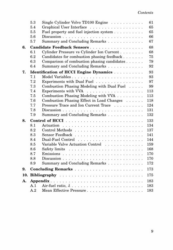
Year
PM All units are in grams per brake horsepower hour
On-Highway Heavy Duty Diesel EngineEmissions standards
NO
x;
NO
x+
HC
;HC
Figure 2.1 U.S. Environmental Protection Agency emissions standards Time-line(http://www.epa.gov/otaq/retrofit/overoh-all.htm).
2.2 Why HCCI?
The first HCCI publication was presented in the late seventies [Onishiet al., 1979; Noguch et al., 1979]. These studies were conducted on two-stroke engines. In the eighties it was shown that HCCI combustion couldalso be achieved on a four-stroke engine [Najt and Foster, 1983]. But it wasnot until the nineties that the area had grown to a large world wide re-search topic [Aoyama et al., 1996; Ryan and Callahan, 1996; Christensenet al., 1997; Hultqvist et al., 1997; Christensen et al., 1999]. One reasonfor the growth of interest is the high demands of the emission levels.In order to meet the upcoming EU and US strict emission legislations,new technology must be used [European Federation for Transport andEnvironment, 2004; U.S. Environmental Protection Agency, 2000]. Bothparticular matter (PM) and NOx need to be significantly decreased (Fig.2.1). In some regards, the HCCI principle incorporates the best featuresof both the SI and the CI engine principles. The mixture is homogenized,which minimizes the particulate emissions and the mixture is compres-sion ignited using high compression ratios, without throttling losses andwith shorter combustion duration, which leads to high efficiency.
The SI principle has low efficiency at part load, where the HCCI hasgood efficiency. The CI engine has similar efficiency as the HCCI engine,but the former generates soot particles and NOx. Especially the NOx emis-sions would be a problem in order to meet the upcoming emission legisla-tion, as it can not be adequately reduced by a three-way catalyst. A NOx
reducing catalyst is today expensive. NOx is mostly dependent on thetemperature during the combustion [Heywood, 1988]. The low emissionsof PM and NOx in HCCI engines are a result of the diluted homogeneousmixture of fuel and air in addition to low combustion temperatures. The
18

2.3 Why Control?
low combustion temperature has two causes. Firstly, since the mixture ishighly diluted the temperature increase due to combustion is moderatesince the fuel must heat a large mass. Secondly, since the mixture is closeto homogeneous there will not be as many hot zones as in a CI engine.
The HCCI engine principle is not limited to a certain fuel, insteadit can be used for a wide range of fuels with different octane numbers[Fiveland et al., 2001].
Does the HCCI principle have any poor features? Currently, there aresome issues to be solved. One issue is that it can produce fairly highconcentrations of unburned hydrocarbon, which needs to be taken care ofby the catalyst. Another is that the promise of fairly high efficiency andlow NOx concentrations is difficult to fulfill when increasing the load. Inorder to run at high load the supercharging needs to be high in order toachieve a diluted charge, which will decrease the overall efficiency dueto increased pumping losses. The pumping losses is the work transferbetween the piston and the cylinder gases during the inlet and exhauststrokes.
Summarizing, HCCI is interesting because it promises low NOx emis-sions and fairly high efficiency.
2.3 Why Control?
In contrast to the SI and CI principle the HCCI principle lacks featuresfor direct control of the combustion phasing. In an SI engine the combus-tion is controlled by the spark plug and in a CI engine the combustionis controlled by direct fuel injection. An HCCI engine have none of theseactuators, hence it is very sensitive to the initial conditions. After theinitial conditions are set, there is no way to affect the combustion phas-ing. Without precise control of temperature, pressure and composition ofthe air/fuel mixture there may be misfire, too high peak pressure or toohigh pressure gradient (dp/dθ ), which could lead to damage of the engineand NOx generation. It is necessary to be able to control the combustionphasing in order to have a large operating range. Even a small variationin the load can change the phasing from too early to too late combustionphasing. The HCCI combustion can also be unstable, resulting in succes-sively earlier (or later) auto-ignition. In this case the wall temperatureacts as a positive feedback and makes the combustion phasing drift away.A higher wall temperature gives an earlier combustion phasing resultingin an even higher wall temperature. Therefore, a fast combustion phasingcontrol is necessary since it sets the performance limitations of the loadcontrol.
19
Chapter 2. Homogeneous Charge Compression Ignition (HCCI)
2.4 Combustion Phasing in HCCI
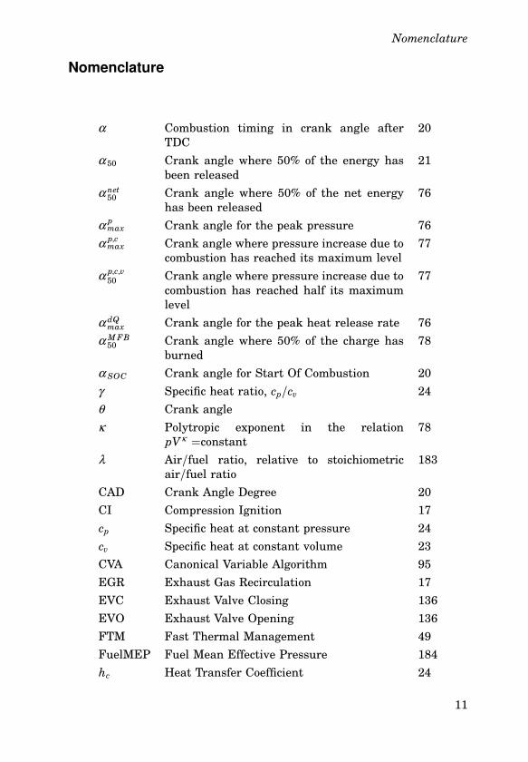
For an HCCI engine it is necessary to control the operating conditions sothat the combustion phasing, α , occurs at a certain crank angle degree(CAD). The combustion phasing can be constant even if the combustionduration varies. As combustion phase expressed in CAD is not enginespeed dependent, the combustion time in seconds is not as important tocontrol as it is to control the combustion phase in CAD. Therefore ,thecombustion phase will be expressed in CAD. Still, the kinetics evolve overtime. The choice of CAD where the combustion should occur, mostly de-pends on the load. When the load increases, the combustion phasing needsto be shifted to a later CAD, since early combustion phasing (close to TopDead Center TDC) gives high peak pressure and high temperature dur-ing the combustion. This will result in faster combustion and at high loadvery rapid combustion causes high mechanical strain on the engine, dueto high peak pressure and high pressure gradients. The high pressure gra-dients cause strain on the engine components, as the pressure wave willreduce the thermal boundary layer at the walls adding positive feedbackon the combustion phasing [Olsson, 2004]. The increased combustion tem-perature increases the heat losses and may lead to NOx emissions. Hence,a short combustion duration at TDC is not always the best solution, evenif it has good theoretical efficiency, as combustion at TDC may generatevery high pressure rates and absolute pressure which could damage theengine.
What is the demand on a sensor used for feedback of combustion phas-ing? To answer that question we need to decide what we mean by combus-tion phasing. The combustion phasing could be defined by several criteria.It could be the crank angle where the maximum pressure during the en-gine cycle occurs. It could be defined as when the start of combustion(α SOC) occurs. Another definition could be the time when a certain per-centage amount of the fuel has been consumed. The CAD of the maximumpressure has the disadvantage that if the combustion occurs very late themaximum pressure can occur at TDC, even if the combustion occurs muchlater. Using α SOC as a definition of the combustion phasing is not a goodchoice since auto-ignition is sensitive to temperature and concentrationsof fuel/air in the mixture and the combustion often start around a similarCAD before we have reached the TDC in cases without misfire. But theduration of the combustion differs a lot. Therefore α SOC does not give agood indication of the combustion phasing. Using the CAD where a certainpercentage amount of the fuel has been burned as indication has benefits,as it is robust measurement at both early and late combustion phasing.But a low percentage such as 10% or 20% has similar problem as α SOC,it does not give the phasing where the combustion rate is highest. How
20

2.5 Modeling of Heat Release
−20 −10 0 10 20−500
0
500
1000
1500
2000
CAD
En
ergy
[J]
Figure 2.2 A heat release curve calculated from cylinder pressure.
much energy that has been released can be found by calculating the heatrelease, see Sec. 2.5 for the calculations. It is found that the heat releaseis fairly symmetric (Fig. 2.2). Hence the crank angle where 50% of theenergy has been released is a good indication of the combustion phasing.It is the median of the combustion, where the combustion rate is highest.This gives a robust indication of the combustion phasing, a small error in50% released energy result in a very small error of the phasing in CAD,since the slope of the energy rate is steep. Hence, for feedback it would besuitable to have a sensor which can be used for estimation of the crankangle where 50% energy has been released. This crank angle has some-times been denoted as CA50 [Olsson et al., 2001b], but in this thesis α 50
will be used as α 50 is better suited notation for mathematical expressions.50% of the energy released is the same as 50% of the fuel burned, and inthe future α 50 is read as the crank angle of 50% burnt. A more detailedstudy of different feedback options is performed in Chapter 6.
2.5 Modeling of Heat Release
The method of monitoring the progression and completeness of the com-bustive reactions, and separating the effect of volume change, heat trans-fer and mass loss based on cylinder pressure is usually referred to as
21

Chapter 2. Homogeneous Charge Compression Ignition (HCCI)
dQhr
dQhr
dQhr
dW
dQcr
dQht
dU
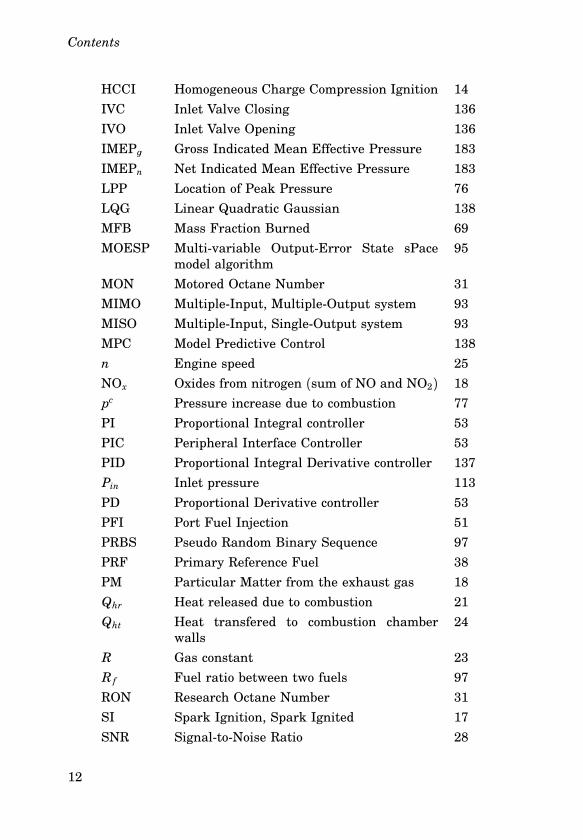
Figure 2.3 Energy balance for an open system with internal chemical heat release.
heat release analysis, and uses the first law of thermodynamics. A per-son familiar to thermodynamics might have objections to the use of theterm heat release, as from a formal thermodynamics point of view, heat istransfered across system boundaries. But in the heat release analysis, itis also included a transformation of fuel energy into thermal energy [Hey-wood, 1988]. In heat release analysis, the time derivative of the enthalpyis calculated relative to some reference state of the cylinder charge.
The purpose of the heat release analysis is to find a method which canbe used for calculation of an scalar combustion phasing variable, α , inreal-time. The model complexity needs to be sufficiently low to allow suf-ficient time in every engine cycle for both calculation of combustion phas-ing and actuation time. Therefore, the model is a trade-off between lowcomplexity and high accuracy. In order to keep the model complexity low,the heat release was modeled using a one-zone model. Hence, we assumethat the temperature and the gas composition are global homogeneous inthe whole cylinder. The model, based on the first law of thermodynamics,has been widely used and model properties have been described earlierin the literature [Gatowski et al., 1984], [Heywood, 1988].
Consider the first law of thermodynamics for an open system:
dU = dQ − dW + hcrdmcr (2.1)
where, dU is the change of internal energy of the mass in the system;Q. is the heat transported into the system; dW is the work performed;hcrdmcr is the energy leakage due to inflow and outflow from crevice re-gions between the piston and the cylinder wall above the piston rings; hcr
is the enthalpy at cylinder condition when dmcr differs from zero; dmcr
22

2.5 Modeling of Heat Release
is the mass flow into and out from the crevice region. The change of heattransported into the system dQ consists of the released energy from thefuel, dQhr and the heat transfered to the chamber walls, dQht. RewritingEq. 2.1 using dQ = dQhr − dQht gives
dQhr = dU + dW + dQht + hcrdmcr (2.2)
We would like to express the heat release in terms of pressure, p,volume, V , and temperature T . The first step is to rewrite the internalenergy term as
dU = mdu + udm = mcvdT + udm (2.3)
where, m is the charge mass; cv is the specific heat at constant volume.By differentiating the ideal gas law, when assuming that the gas constantR is constant, dT can be expressed in p,V , and m
pV = mRT (2.4)
dpV + pdV = mRdT + dmRT (2.5)
with p being pressure, V volume and R gas constant. Hence, dU can bewritten as
dT =1
mR(dpV + pdV) −
T
mdm ; (2.6)
dU =cv
R(dpV + pdV) + udm − cvTdm (2.7)
The second step is to rewrite the work performed as
dW = pdV (2.8)
Using Eq. (2.7) and Eq. (2.8), Eq. (2.2) can be written as
dQhr =cv
R(dpV + pdV) + pdV + dQht + udm − cvTdm + hcrdmcr
= (1 +cv
R)pdV +
cv
RVdp + dQht + udm − cvTdm + hcrdmcr (2.9)
The crevice effect is modeled as a single volume at the cylinder pressureto simulate the piston/ring/cylinder-wall region. A mass balance gives
dm = −dmcr ; (2.10)
dQhr = (1 +cv
R)pdV +
cv
RVdp + dQht + (u − cvT + hcr)dmcr (2.11)
23

Chapter 2. Homogeneous Charge Compression Ignition (HCCI)
For ideal gas the relation between cv, cp and R is
cp = cv + R (2.12)
where cp is the specific heat at constant pressure. Assuming that thechanges are quantified per crank angle degree, we choose crank anglesince our system will be crank angle based. Eq. (2.11) is then written as
dQhr
dθ=
γ
γ − 1p
dV
dθ+
1γ − 1
Vdp
dθ+
dQht
dθ+ (u − cvT + hcr)
dmcr
dθ
=γ
γ − 1p
dV
dθ+
1γ − 1
Vdp
dθ+
dQht
dθ+
dQcr
dθ(2.13)
where γ is the specific heat ratio defined by
γ =cp
cv
(2.14)
The specific heat ratio γ , depends on gas composition and temperature.There is not a linear relationship between γ and temperature, [Heywood,1988], but a simple and fairly accurate model is to assume a relationshipas
γ (T) = a + bT (2.15)
given that the enthalpy is related to the internal energy as
h = u + pv (2.16)
The third term, the heat transfer rate to the combustion chamber walls,Qht, can be calculated from the relation
dQht
dt= hc Aw(T − Tw) (2.17)
where hc is the heat transfer coefficient, Aw is the chamber wall area, Tw
is the mean wall temperature, and hc can be estimated using Nusselt-Reynold numbers. The heat transfer coefficient is estimated by using re-sult from [Woschni, 1967] who assumed a correlation of the form
Nu = 0.0035 ⋅ Re0.8 (2.18)
where Nu is the Nusselt number, Re is the Reynolds number. Then is hc
given by
ω = 2.28(
2Sn + 3.24 ⋅ 10−3C2
(Vd
VIV C
) (p − pm
pIV C
)TIV C
)(2.19)
hc = 131C1 B−0.2p0.8T−0.55ω 0.8 (2.20)
24

2.6 HCCI Combustion
where Vd is the displaced volume, VIV C is the volume at inlet valve clos-ing (IVC), pm is the motored cylinder pressure, pIV C is the pressure atIVC, TIV C is the temperature at IVC, C1 and C2 are motor dependent con-stants, B is the cylinder bore, S is the stroke and n is the engine speedin revolutions per second.
The energy due to the crevice effect, Qcr, can be modeled using the factthat the crevice regions are narrow. Therefore an appropriate assumptionis that the aggregate crevice volume has the same gas temperature as thewalls and the same pressure as the cylinder,
mcr = pVcr/RTw (2.21)
where Tw is the wall temperature. We rewrite the term which is multipliedwith mcr as
hcr − u + cvT = ucr + pcrvcr − u + cvT = ucr − u + R(T cr +T
γ − 1) (2.22)
The difference u − ucr, using γ (T) = a + bT , can then be expressed as
ucr − u =∫ T
T cr cvdT = − Rb
ln(
γ −1γ cr−1
)(2.23)
The heat transfer due to crevice effect, dQcr, can then be written as
dQcr =Vcr
Tw
(T cr +
T
γ − 1−
1b
ln(
γ − 1γ cr − 1
))dp (2.24)
using Eq. (2.21) and Eq. (2.23). The crevice effect on the heat release isvery small, a few percent of the total energy. Hence, crevice effects areoften neglected in heat release calculations and at least in the case whenthe objective is to control the combustion, this simplification is justified.
2.6 HCCI Combustion
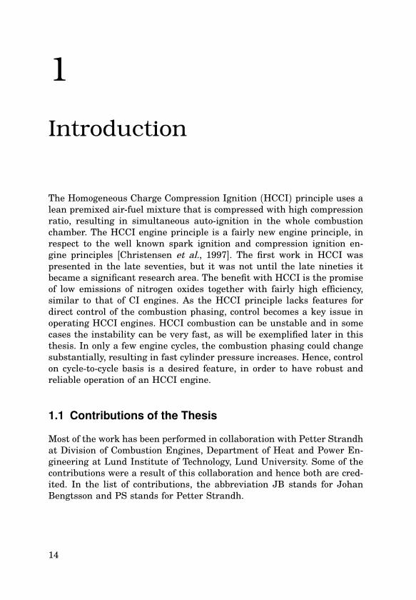
HCCI combustion differs from SI and CI combustion, since the combustionoccurs globally and is very fast. Therefore, the time for the combustionneeds to be controlled to avoid fast pressure rise, pressure oscillations andhigh maximum pressure. In Fig. 2.4, a pressure trace with correspondingheat release is shown. It can be observed that the combustion durationis short, the heat release of 10% to 90% burned is reached approximatelyaround 5 CAD. This can be compared with SI, where the combustionduration is around 30-40 CAD, and CI, where the combustion duration is
25

Chapter 2. Homogeneous Charge Compression Ignition (HCCI)
−20 −10 TDC 10 20 30 400
1.6
3.2
4.8
6.4
8x 10
6
−20 −10 TDC 10 20 30 400
360
720
1080
1440
1800P
ress
ure
[Pa]
En
ergy
[J]
Crank angle [CAD]
Figure 2.4 Cylinder pressure trace of a motored cycle (dash-dotted), burned cycle(solid) and the heat release of the burned cycle (dashed).
around 60-90 CAD [Heywood, 1988]. From the figure, the mixture effect onthe pressure trace can also be observed. In the motored cycle the mixtureconsists of only air and in the burned cycle the mixture consisted of fueland air. The mixtures have different ratio of specific heats, which resultsin that the pressure trace during the compression will differ for the twomixtures. The temperature for these two pressure traces were almost thesame, since there were only three engine cycles between them and theengine was operated at 1200 rpm during the experiment. In Fig. 2.5, ap-V diagram of an engine cycle is shown. It can be observed that thepumping losses are small, this is due to that an HCCI engine is operatedunthrottled. It can also be observed that the combustion phasing of thiscycle occur not at TDC, but a few CAD after TDC. It is desired to maximizethe work performed and therefore having the combustion to occur closeto TDC. But combustion close to TDC will lead to high peak pressure,pressure oscillations and possibly damage to the engine and therefore alater combustion phasing was chosen. During the compression cycle andthe expansion cycle after the combustion is finished, no chemical reactions
26

2.6 HCCI Combustion
0 0.5 1 1.5 2 2.5
x 10−3
0
20
40
60
80
100
120
140
160
180
Volume [m3]
Pre
ssu
re[a
tm]
Figure 2.5 Pressure-volume curve of a full engine cycle.
take place and Eq. (2.9) is simplified to
0 = dQhr =cv
RV dp +
cp
RpdV − dQht (2.25)
dQht can be defined as
dQht = aV dp + bpdV (2.26)
for this certain type of process, where a and b are functions of temperature[Tunestål, 2001]. Eq. (2.25) is then rewritten as
dp
p= −κ
dV
V(2.27)
with
κ =
cv
R− b
cp
R− a
27
Chapter 2. Homogeneous Charge Compression Ignition (HCCI)
10−4
10−3
100
101
102
103
Volume [m3]
Pre
ssu
re[a
tm]
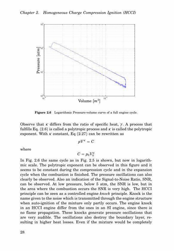
Figure 2.6 Logarithmic Pressure-volume curve of a full engine cycle.
Observe that κ differs from the ratio of specific heat, γ . A process thatfulfills Eq. (2.6) is called a polytropic process and κ is called the polytropicexponent. With κ constant, Eq (2.27) can be rewritten as
pVκ = C
whereC = p0Vκ
0
In Fig. 2.6 the same cycle as in Fig. 2.5 is shown, but now in logarith-mic scale. The polytropic exponent can be observed in this figure and itseems to be constant during the compression cycle and in the expansioncycle when the combustion is finished. The pressure oscillations can alsoclearly be observed. Also an indication of the Signal-to-Noise Ratio, SNR,can be observed. At low pressure, below 5 atm, the SNR is low, but inthe area where the combustion occurs the SNR is very high. The HCCIprinciple can be seen as a controlled engine knock principle. Knock is thename given to the noise which is transmitted through the engine structurewhen auto-ignition of the mixture only partly occurs. The engine knockin an HCCI engine differ from the ones in an SI engine, since there isno flame propagation. These knocks generate pressure oscillations thatare very audible. The oscillations also destroy the boundary layer, re-sulting in higher heat losses. Even if the mixture would be completely
28

2.6 HCCI Combustion
1700 1750 1800 1850 1900 1950 20000.8
0.9
1
1.1
1.2
1.3
1.4
1.5
1.6
1.7
1.8x 10
7
Pre
ssu
re[P
a]
CAD
Figure 2.7 Pressure trace with oscillations
homogeneous, there would be knock since the temperature still would notbe spatially uniform. For example, the cylinder wall has impact on thein-cylinder temperature. As the kinetics start the temperature becomesinitial spatially almost uniform as a result of the temperature inversionof the reactivity, but regions having different chemical composition mayexist [Griffiths and Whitaker, 2002]. This will lead to that the combustionwill not be completely spatially uniform and knock may occur. There arealso studies in order to predict when knock may occur [Yelvington andGreen, 2003; Oakley et al., 2001; Vressner et al., 2003]. Fig. 2.7 showsan example of the pressure oscillations in an HCCI engine. Even if thecycle-to-cycle variations of an HCCI is lesser than for SI and CI principles,there still is a significant variation (Fig. 2.8). The variation depends onoperating condition.
29

Chapter 2. Homogeneous Charge Compression Ignition (HCCI)
−30 −20 −10 0 10 20 302
4
6
8x 10
6
4 4.5 5 5.5 6 6.5 7 7.50
50
100
Occ
urr
ence
sP
ress
ure
[Pa]
CAD
Combustion phasing [CAD]
Figure 2.8 Cycle-to-cycle variations at open-loop control. Upper figure shows thepressure traces and the lower shows a histogram of the combustion phasing.
2.7 Emissions
Nitrogen Oxides
The NO formation is exponentially dependent on the temperature and in-cylinder combustion temperatures above 1800 K results in NO formation[Heywood, 1988; Christensen et al., 1997]. HCCI combustion results in lowcombustion temperature, since the premixed mixture is highly diluted,and no or very low NOx emissions are formed.
Hydrocarbons
The HC emissions are the result of incomplete combustion of the mixture.The emissions are a result of the low combustion temperature. The lowtemperature makes the HCCI combustion sensitive to flame quenching atthe chamber walls and crevice regions. The levels of HC have effect onthe overall engine efficiency [Christensen, 2002].
Carbon Monoxide
The source of CO is fuel that oxidizes late enough for the mixture to freezebefore CO is further oxidized to CO2. The formation of CO is temperature
30
2.8 Efficiency
dependent and a higher temperature will decrease the formation. CO for-mation decrease when the combustion phasing is advanced due to highertemperature and longer time for oxidation, but such conditions will resultin increased NOx formation [Christensen, 2002].
2.8 Efficiency
An HCCI engine is operated unthrottled and can use high compressionratio, which gives good fuel conversion efficiency. The HCCI combustiontemperature is low, but even so there are significant heat losses due tocombustion close to the chamber walls and due to the in-cylinder pres-sure oscillations. At high load the combustion phasing must be retardedin order to keep the in-cylinder temperature and pressure at acceptablelevels. Late combustion phasing also have negative impact on the engineefficiency, since there will be loss in the performed work of the engine.The HCCI engine has an engine efficiency similar to the Diesel engine[Christensen, 2002].
2.9 Fuel Properties
An HCCI engine can be operated on a wide range of fuels, but the fuelshave different properties which have significant effects on the operationrange [Christensen et al., 1997]. The fuel properties should be such thatthe engine can run in HCCI mode both at low and high load. Since thebenefits with HCCI decrease at high load, the fuel could be used for SI op-eration. There are several studies on the characteristics of different fuelsin an HCCI engine, to obtain a fuel which is suitable for HCCI [Tanakaet al., 2003b; Dec and Sjöberg, 2004; Sjöberg and Dec, 2003; Jeuland et al.,2004]. The octane numbers–Research Octane Number (RON) and MotorOctane Number (MON)–are used to characterize fuel for SI engines andcetane number to characterize fuel for CI engines. Whereas RON, MONand cetane may have no relevance to characterize HCCI combustion, itremains important to find effective characterizations of HCCI fuel prop-erties. HCCI engines have requirements on the fuel that differ from otherengines and a fuel specification of HCCI combustion should be developed.Fuels with similar octane number may have s different HCCI combustion,the formation of the fuel has significant effect on the combustion [Sjöbergand Dec, 2003]. In [Tanaka et al., 2003b] a control scheme for controllingignition delay, maximum dp and burn rate was proposed, but practicallyit can only be used to shorten ignition delay and faster burn rate. In HCCI
31

Chapter 2. Homogeneous Charge Compression Ignition (HCCI)
combustion the challenge is mostly to obtain the opposite, longer ignitiondelay and slower burn rate.
2.10 Scientific Challenges
The scientific challenges with HCCI are to control the combustion at awide operation range and simultaneously have fairly high efficiency andlow concentrations of NOx, HC and CO. To fulfill these requirements, sev-eral barriers must be overcome before HCCI engines can reach production.
Deriving Dynamic Models of HCCI Combustion
There is a need of models suitable for control design. The HCCI combus-tion is very complex, even so a model useful for control design purposesneeds to be dynamically accurate, yet preferably simple and not withhundreds of states. Full kinetic models of the HCCI combustion may beneeded to understand the kinetics in the combustion. If accurate and dy-namically precise, these models can be used for evaluation of the controlperformance and simulation of the combustion.
Sensor and actuator study
For commercial success, cheap sensors that can measure the combustionphasing, which are reliable and have long lifespan need to be found. To-day’s cylinder pressure transducers are too expensive and have too shortlife-span for production. At the moment, ion current sensors are not re-liable in the whole operating range for HCCI. There are several possibleactuators for controlling the HCCI dynamics and more studies are neededin order to show the actuators fully potential in controlling the HCCI dy-namics.
Development of Direct Injection System for HCCI
If diesel is going to be used as fuel, there is a need to develop directinjection system, where homogeneous mixture can be obtained and stillstart the injection close to TDC. This is mostly a challenge in developingHCCI engines for heavy trucks in the short run.
Control of the Combustion Phasing
To control the combustion phasing in the whole HCCI mode range (i.e.,for various loads, speeds and temperatures) is a challenge, as the HCCIprinciple lacks features for direct combustion phasing. A precise and fastcontrol of combustion phasing is needed in order to fulfill good efficiency,load control and low emissions.
32

2.10 Scientific Challenges
Control at High Load
A HCCI engine needs to be able to operate at a load range similar to theSI or CI engine principles. At high load the combustion rate is very highresults in very high pressure increases, pressure oscillations and absolutepressure. This limits the efficiency and puts high structural demands onthe engine. Research is needed to further understand how to slow thekinetics and achieve longer combustion duration.
Control of the Noise Level
The engine knock generates an audible manifestation which is commer-cially unacceptable. This issue is related to control at high load.
Control of Emissions
The level of the emissions need to be controlled, still with an acceptableoverall efficiency. The exhaust temperature from HCCI combustion is lowand development of oxidation catalysts for low-temperature exhaust areneeded to meet the future emission standards for HC and CO.
Fuel Characterization for HCCI Combustion
The fuel has strong effects on the HCCI combustion and a classificationof fuel effects on HCCI combustion is needed.
Cold-start
The HCCI engine has cold-start difficulties, the temperature of the mix-ture is not high enough to auto-ignite. Today the most practical approachis to start the engine in another standard operation mode as CI or SI andto switch to HCCI mode after warm-up.
33
3
Physical Modeling of HCCI
Engine Dynamics
In homogeneous charge compression ignition (HCCI) engines the combus-tion phasing is determined by the autoignition properties of the air-fuelmixture in use. Small variations in the cylinder environment may greatlyinfluence the combustion phasing [Hyvönen et al., 2004]. In order to con-trol engine operation it is therefore necessary to have good models andsubstantial understanding of the ignition and combustion process. Thiswork aims at describing the major thermodynamic and chemical interac-tions in the course of an engine stroke and their influence on combustionphasing. The goal is to construct a simulation model that (qualitatively)reproduces HCCI engine operation for the purpose of synthesizing, an-alyzing, and evaluating various combustion phasing control strategies.This chapter is a feasibility study on requirements and choice of com-plexity level for a suitable model, and is to be regarded as a first steptowards a complete model. The proposed model structure consists of azero-dimensional cylinder model, combined with a reduced chemical ki-netic model to describe the ignition process. Experiments on a real enginewith dual fuels and inlet air temperature control have been conductedto collect information on the phenomena to reproduce and to compare tosimulated results.
Experiments
The experimental setup consisted of a heavy duty Volvo diesel engine,Table 3.1, and the set-up will in more detail be described in Sec. 5.1. In theexperiments, the fuel ratio, R f , of the dual fuels ethanol and n-heptane,fuel energy per cycle, Qin, inlet air temperature, Tin, and the engine speed,n, were changed according to Table 3.2. By changing the injected fuelenergy per cycle the load is changed and Qin = 1000 J corresponds to
34

3.1 Model
Table 3.1 Engine specifications.
Operated cylinders 6
Displaced Volume 2000 cm3
Bore 131 mm
Stroke 150 mm
Connecting Rod Length 260 mm
Number of Valves 4
Compression Ratio 18.5:1
Fuel Supply port fuel injection
Table 3.2 Experimental conditions
Tin [C] 100–115 100 100 100
n[rpm] 1200 1000–1500 1200 1200
Qin[J] 1400 1400 1000–1500 1400
R f [vol%] 0.93 0.93 0.93 0.892–1.0
a FuelMEP (Fuel Mean Effective Pressure, see Sec. A.2) of 5 bar andQin = 1500 J corresponds to a FuelMEP of 7.5 bar. As the engine wasnaturally aspirated this corresponds to that λ , air/fuel ratio, varied from6.2 to 4.1. Only low load experiments in open loop were performed, whenthe engine temperature was at steady state. At each operating point,data of 500 cycles were collected. The mean value of these 500 cycles wasthereafter used in comparison with the result from the model.
3.1 Model
HCCI combustion is often achieved without a complete homogeneous mix-ture. But in order to derive a control-relevant model, we might firstlyproceed by assuming that the mixture is homogeneous, thus allowing asingle-zone cylinder model. Such assumption may be justified by laser-diagnostic measurements [Richter et al., 2000]. To reproduce the effectsrelevant for combustion phasing control it is required that the autoignitionmodel captures the effects on ignition delay (induction time) of varying
35

Chapter 3. Physical Modeling of HCCI Engine Dynamics
species concentrations, temperature trace, and fuel quality. Several alter-native approaches are possible for modeling the instant of autoignition forfuels. Large models, e.g. [Sjöberg and Dec, 2003] (PRF fuels, 857 species,3,606 reactions, CHEMKIN/LLNL), have been used to model completecombustion. In addition to ignition prediction, such models are also aimedat describing intermediate species and end product composition. Reducedchemical kinetics models, e.g. [Tanaka et al., 2003a] (PRF fuels, 32 species,55 reactions, CHEMKIN), have also been proposed, where reactions withlittle influence on the combustion have been identified and removed. Forsimulation of multi-cycle scenarios it is necessary to keep the model com-plexity low in order to arrive at reasonable simulation times. An attrac-tive and widespread alternative is to use the Shell model [Halstead et al.,1977], which is a lumped chemical kinetics model using only five represen-tative species in eight generic reactions. This model is aimed at predictionof autoignition rather than describing the complete combustion process.Compression ignition delay may also be described by empirical correla-tions, such as the knock integral condition
∫ ti
t=0
dt
τ= 1 (3.1)
where ti is the instant of ignition and τ is the estimated ignition time(ignition delay) at the instantaneous pressure and temperature condi-tions at time t, often described by Arrhenius type expressions [Heywood,1988]. A drawback is that dependence on species concentrations is nor-mally not regarded. An integral condition with concentration dependencewas used in [Shaver et al., 2003; Shaver et al., 2004] in a similar studyfor propane fuel, where also autoignition models based on very simplereaction mechanisms were evaluated. Alternatives to physical or physicalbased models are to use system identification to obtain models or to useempirical look-up tables. The latter gives very little physical insight, andrequire substantial efforts to calibrate. In this work, the Shell model waschosen to describe the process of autoignition. A static model is then usedto describe the major part of the actual combustion and correspondingheat release. The result from the Shell model is compared with resultfrom an integrated Arrhenius rate threshold model.
Cylinder Model
The cylinder gas dynamics are described by the first law with volume-pressure work
δ QH R = (1 +cv
R)pdV +
cv
RVdp + δ QHT (3.2)
36

3.1 Model
where p is the cylinder pressure, V the volume, Ru the universal gasconstant, cv = cp−Ru the specific heat capacity, and n the molar substanceamount contained in the cylinder. The time derivatives of QH R and QHT
denote rates of heat released by the combustion process and heat flowingfrom the wall.
Gas Properties
The gas is described as a mixture of dry air and fuel, and the combustionproducts are nitrogen, carbondioxide and water. Specific heat for eachspecies i is described by NASA polynomial approximations of JANAF data
cp,i(T) =Ru
Mi
5∑
j=1
ai, j Tj−3 (3.3)
where Mi is the molar mass of species i and T is the cylinder temperature.The mixture specific heat is then
cp(T) =1n
∑
i
niMicp,i(T) (3.4)
where ni is the mole of species i.
Shell Autoignition Model
The Shell autoignition model for hydrocarbon fuels [Halstead et al., 1977],Ca Hb, is based on a general eight-step chain-branching reaction schemewith lumped species: The hydrocarbon fuel RH, radicals R, intermediatespecies Q, and the chain branching agent B.
RH + O2kq
−→ 2R (initiation) (3.5)
Rkp
−→ R + products and heat (propagation cycle) (3.6)
Rf1 kp
−→ R + B (propagation forming B) (3.7)
R + Qf2 kp
−→ R + B (propagation forming B) (3.8)
Rf3 kp
−→ out (linear termination) (3.9)
Rf4 kp
−→ R + Q (propagation forming Q) (3.10)
2Rkt
−→ out (quadratic termination) (3.11)
Bkb
−→ 2R (degenerate branching) (3.12)
37

Chapter 3. Physical Modeling of HCCI Engine Dynamics
Autoignition is described by integrating the time variations of speciesconcentrations from the beginning of the compression stroke.
d[R]
dt= 2
kq[RH][O2] + kb[B] − kt[R]
2
− f3kp[R] (3.13)
d[B]
dt= f1kp[R] + f2kp[Q][R] − kb[B] (3.14)
d[Q]
dt= f4kp[R] − f2kp[Q][R] (3.15)
d[O2]
dt= −nkp[R] (3.16)
The species R, Q, and B are not considered in thermodynamic computa-tions for the gas mixture. The stoichiometry is approximated by assuminga constant CO/CO2 ratio, ν , for the complete combustion process, withoxygen consumption n = 2[a(1 − ν) + b/4]/b mole per cycle. The heatrelease from combustion is given by
dQH R
dt= kpqV [R] (3.17)
where q is the exothermicity per cycle for the regarded fuel. The propa-gation rate coefficient is described as
k−1p =
1kp,1[O2]
+1
kp,2+
1kp,1[RH]
(3.18)
To capture dependence of induction periods on fuel and air concentrationsthe terms f1, f3, and f4 are expressed as
f i = f i [O2]xi [RH]yi (3.19)
Rate coefficients and rate parameters ki and f i are then described by
Arrhenius rate coefficients
ki = Ai exp[
Ei
RuT
], f
i = Ai exp[
Ei
RuT
](3.20)
Calibrated parameters for a number of fuels, including a set of PrimaryReference Fuels (PRF), are found in the literature [Halstead et al., 1977].PRFx is a mixture of n-heptane and iso-octane, where the octane numberx is defined as the volume percentage of iso-octane. Parameters for PRF90were used in the simulations. Autoignition was defined as the crank anglewhere the explosive phase of combustion starts.
38
3.1 Model
Integrated Arrhenius Rate Threshold
The Arrhenius form can be used to determine the rate coefficient de-scribing a single-step reaction between two molecules [Thurns, 1996]. Thesingle-step rate integral condition is based on the knock integral with
Kth =
∫ θ
θ IVC
1/τ dθ/w (3.21)
1/τ = A exp(Ea/(RuT))[Fuel]a[O2]b (3.22)
where θ is the crank angle and θ IVC is the cank angle of the inlet valveclosure. The integral condition describes a generalized reaction of fueland oxygen and this is an extreme simplification of the large number ofreactions that take place during combustion. The empirical parameters A,Ea, a, b and Kth are determined from experiments. Values for n-heptaneand iso-octane from [Thurns, 1996] was used in the comparison below.Autoignition was defined as the crank angle where the integral conditionhas reached the threshold Kth.
Combustion
When autoignition is detected by the Shell model or the Integrated Ar-rhenius Rate Threshold, the completion of combustion is described by aWiebe function [Vibe, 1970].
xb(θ ) = 1 − exp[−a(
θ − θ0
∆θ)m+1
](3.23)
where xb denotes the mass fraction burnt, θ is the crank angle, θ0 start ofcombustion, ∆θ is the total duration, and a and m adjustable parametersthat fix the shape of the curve. The heat release is computed from therate of xb and the higher heating value of the fuel.
Heat Transfer
Heat is transfered by convection and radiation between in-cylinder gasesand cylinder head, valves, cylinder walls, and piston during the enginecycle. In this case the radiation is neglected. This problem is very complex,but a standard solution is to use the Newton law for external heat transfer
dQW
dt= hc AW(T − TW) (3.24)
where QW is the heat transfer by conduction, AW is the wall area, TW isthe wall temperature, and the heat-transfer coefficient, hc, is given by theNusselt-Reynold relation by Woschni [Woschni, 1967].
hc = 3.26B−0.2p0.8T−0.55(2.28Sp)0.8 (3.25)
39
Chapter 3. Physical Modeling of HCCI Engine Dynamics
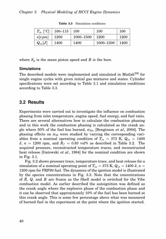
Table 3.3 Simulation conditions
Tin [C] 100–115 100 100 100
n[rpm] 1200 1000–1500 1200 1200
Qin[J] 1400 1400 1000–1500 1400
where Sp is the mean piston speed and B is the bore.
Simulations
The described models were implemented and simulated in MatlabTM forsingle engine cycles with given initial gas mixtures and states. Cylinderspecifications were set according to Table 3.1 and simulation conditionsaccording to Table 3.3.
3.2 Results
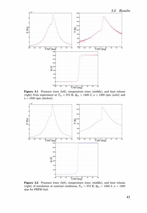
Experiments were carried out to investigate the influence on combustionphasing from inlet temperature, engine speed, fuel energy, and fuel ratio.There are several alternatives how to calculate the combustion phasingand in this work the combustion phasing is calculated as the crank an-gle where 50% of the fuel has burned, α 50, [Bengtsson et al., 2004]. Thephasing effects on α 50 were studied by varying the corresponding vari-ables from a nominal operating condition of Tin = 373 K, Qin = 1400J, n = 1200 rpm, and R f = 0.93 vol% as described in Table 3.2. Theacquired pressure, reconstructed temperature traces, and reconstructedheat release [Gatowski et al., 1984] for the nominal condition are shownin Fig. 3.1.
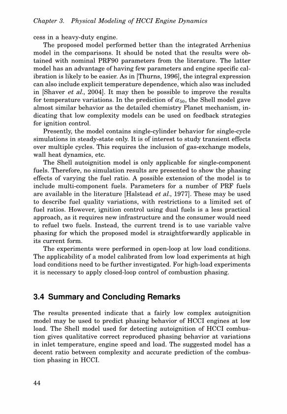
Fig. 3.2 shows pressure trace, temperature trace, and heat release for asimulation of a nominal operating point of Tin = 373 K, Qin = 1400 J, n =1200 rpm for PRF90 fuel. The dynamics of the ignition model is illustratedby the species concentrations in Fig. 3.3. Note that the concentrationsof R, Q, and B are frozen as the Shell model is switched for the Vibecombustion model. As earlier described the autoignition was defined asthe crank angle where the explosive phase of the combustion phase andit can be observed that approximately 10% of the fuel has been burned atthis crank angle. This is some few percentage above what was measuredof burned fuel in the experiment at the point where the ignition started.
40
3.2 Results
−80 −60 −40 −20 0 20 40 60 800
1
2
3
4
5
6
7x 10
6
CAD [deg]
P[P
a]
−80 −60 −40 −20 0 20 40 60 80200
400
600
800
1000
1200
1400
1600
1800
CAD [deg]
T[K
]
−80 −60 −40 −20 0 20 40 60 80−200
0
200
400
600
800
1000
1200
1400
1600
CAD [deg]
Q[J
]
Figure 3.1 Pressure trace (left), temperature trace (middle), and heat release(right) from experiment at Tin = 373 K, Qin = 1400 J, n = 1200 rpm (solid) andn = 1500 rpm (dashed).
−80 −60 −40 −20 0 20 40 60 800
1
2
3
4
5
6
7
x 106
CAD [deg]
P[P
a]
−80 −60 −40 −20 0 20 40 60 80200
400
600
800
1000
1200
1400
1600
CAD [deg]
T[K
]
−80 −60 −40 −20 0 20 40 60 80
0
200
400
600
800
1000
1200
1400
CAD [deg]
Q[J
]
Figure 3.2 Pressure trace (left), temperature trace (middle), and heat release(right) of simulation at nominal conditions, Tin = 373 K, Qin = 1400 J, n = 1200rpm for PRF90 fuel.
41

Chapter 3. Physical Modeling of HCCI Engine Dynamics
−150 −100 −50 0 50 100 15010
−20
10−15
10−10
10−5
100
−150 −100 −50 0 50 100 15010
−20
10−15
10−10
10−5
100
nRH
nR
nB
nQ
nAir
nCO2
nH2O
nN2
n[m
ol]
n[m
ol]
θ [deg]
θ [deg]
Figure 3.3 Concentrations of gas species from Shell model ignition dynamics fornominal conditions, Tin = 373 K, Qin = 1400 J, n = 1200 rpm for PRF90 fuel.
Phasing effects on α 50 from variations of inlet temperature, fuel en-ergy and engine speed according to Tables 3.2 and 3.3 are summarizedin Fig. 3.4. It can be noted that the Shell model gives quite accurate es-timation of the phasing for the temperature and the engine speed sweep.The model is slightly less accurate when changing the load, but still givesthe correct trend.
Results from simulations using the integrated Arrhenius model arealso shown in Figure 3.4. This method gives good results for load varia-tions. The results for speed variations are less accurate at higher speeds.However, the model fails at variations of the inlet temperature.
In order to compare the ignition prediction accuracy of these low com-plexity models with more refined ones, results from homogeneous calcula-tions using detailed chemical kinetics are included in Figure 3.4. Here, de-tailed chemistry for an ethanol/n-heptane mixture was obtained throughthe Planet mechanism for PRF fuels. For more details on the physical andchemical modeling, see references [Amnéus, 2002; Ahmed et al., 2003].From Figure 3.4 it can be observed that the Shell model gives similar re-sults of prediction of α 50 as the Planet mechanism for inlet temperature
42

3.3 Discussion
100 105 110 1150
2
4
6
8
10
1000 1100 1200 1300 1400 15000
5
10
15
20
1000 1100 1200 1300 1400 15004
6
8
10
12
14
16
18
α50
[deg
]
α50
[deg
]
α50
[deg
]
Tin [deg Celsius] n [rpm]
Qin [J]
Figure 3.4 Effects on combustion phasing of variations from nominal conditions,Tin = 373 K, Qin = 1400 J, n = 1200 rpm. The experimental results are markedas ’*’, the Shell model results with ’o’, the Arrhenius Rate Integral results with ’+’,and the Planet mechanism with ’♦’.
variations. This observation is also true for the speed variations. But inthe case of load variation the Planet mechanism gives significantly betterresult.
3.3 Discussion
The results indicate that the proposed model may be used for studieson feedback strategies for ignition control. Qualitative phasing behavioris correctly reproduced at variations in inlet temperature, engine speed,and load.
The simulation model was only crudely calibrated and the quantita-tive results are expected to improve with calibration. The Shell-modelparameters of [Halstead et al., 1977] are from experiments on a rapidcompression machine. Preliminary attempts with manual tuning of theparameters have shown to yield better agreement with the ignition pro-
43
Chapter 3. Physical Modeling of HCCI Engine Dynamics
cess in a heavy-duty engine.The proposed model performed better than the integrated Arrhenius
model in the comparisons. It should be noted that the results were ob-tained with nominal PRF90 parameters from the literature. The lattermodel has an advantage of having few parameters and engine specific cal-ibration is likely to be easier. As in [Thurns, 1996], the integral expressioncan also include explicit temperature dependence, which also was includedin [Shaver et al., 2004]. It may then be possible to improve the resultsfor temperature variations. In the prediction of α 50, the Shell model gavealmost similar behavior as the detailed chemistry Planet mechanism, in-dicating that low complexity models can be used on feedback strategiesfor ignition control.
Presently, the model contains single-cylinder behavior for single-cyclesimulations in steady-state only. It is of interest to study transient effectsover multiple cycles. This requires the inclusion of gas-exchange models,wall heat dynamics, etc.
The Shell autoignition model is only applicable for single-componentfuels. Therefore, no simulation results are presented to show the phasingeffects of varying the fuel ratio. A possible extension of the model is toinclude multi-component fuels. Parameters for a number of PRF fuelsare available in the literature [Halstead et al., 1977]. These may be usedto describe fuel quality variations, with restrictions to a limited set offuel ratios. However, ignition control using dual fuels is a less practicalapproach, as it requires new infrastructure and the consumer would needto refuel two fuels. Instead, the current trend is to use variable valvephasing for which the proposed model is straightforwardly applicable inits current form.
The experiments were performed in open-loop at low load conditions.The applicability of a model calibrated from low load experiments at highload conditions need to be further investigated. For high-load experimentsit is necessary to apply closed-loop control of combustion phasing.
3.4 Summary and Concluding Remarks
The results presented indicate that a fairly low complex autoignitionmodel may be used to predict phasing behavior of HCCI engines at lowload. The Shell model used for detecting autoignition of HCCI combus-tion gives qualitative correct reproduced phasing behavior at variationsin inlet temperature, engine speed and load. The suggested model has adecent ratio between complexity and accurate prediction of the combus-tion phasing in HCCI.
44

4
Sensors and Actuators for
HCCI Control
In this thesis, control was an objective all from the beginning and therewere few limitations of which sensors should be used. The HCCI combus-tion depend on for example temperatures, pressures and engine speed.Therefore, sensors are vital in control of HCCI engines. The combustionphasing signal is the most important measurement, but other sensorsmeasuring the state of the engine are also important. For example, thetemperature of the exhaust gas gives indication of state of the engine.The sensor measuring the combustion phasing need to have high band-width as it measure the ongoing combustion, and the combustion phasingis preferably used for cycle-to-cycle control. The actuator must be capa-ble of cylinder individual control of the engine in a large operating range.This chapter discusses the sensors available today and actuators for HCCIfeedback control.
4.1 Sensors
The sensors may be divided into two classes, the ones which are usedfor measuring the on-going combustion and the ones which measure theresult of the combustion and the engine state, measuring on cycle-to-cycle basis or slower. The sensor demands differs, both from a bandwidthand environmental point of view and hence the division. The purpose formeasuring the on-going combustion is to estimate the combustion phasing,α , which is needed to control the HCCI combustion.
Combustion Phasing Sensors
Combustion phasing sensors provide feedback on the current combustionlapse. The sensor technologies for combustion phasing have not been thor-
45
Chapter 4. Sensors and Actuators for HCCI Control
oughly investigated by the author, as only some of the various technologieshave been used.
Piezo-Electric Pressure Transducer The transducer works by emit-ting an electronic signal proportional to the deflection of a diaphragmwhen exposed to cylinder pressures. The transducer is able to measurechanges in the pressure, but not absolute measurement. Absolute mea-surement can be obtained by estimation of the offset. The transducer hasa wide frequency response and is linear over a large range. The pres-sure transducer could measure the full cylinder pressure trace or onlythe peak pressure. A peak pressure sensor traditionally measures thepressure through the cylinder block, resulting in distortion of the phase.Still, it can approximately estimate the peak pressure. Today there existseveral low-cost piezo transducers [Sellnau et al., 2000; Shimasaki et al.,2004]. The accuracy of these low-cost sensors is probably sufficient forfeedback control of HCCI combustion phasing.
Optical Pressure Transducer Measuring the light intensity reflectedfrom a metal diaphragm. The sensing element of the pressure transduceris essentially a Fabry-Pérot type optical interferometer. The geometry andmaterial of the transducer are selected in order to obtain a linear relation-ship between the deflection of the diaphragm and the applied pressure.Currently, the optical pressure transducers are less accurate than the bestpiezo-electric pressure transducers [Roth et al., 2002].
Ion Current An alternative to the use of the pressure transducers isto use the electronic conductive properties for the reaction zone. The phe-nomenon is called ion current for which no expensive sensor is needed,instead a standard spark plug can be used [Gillbrand et al., 1987; Rein-mann, 1998; Eriksson et al., 1997]. The basic principle of ion currentsensing is that a voltage is applied over an electrode gap inserted into theactual gas volume (combustion chamber). In a non-reacting charge, no ioncurrent through the gap will be present. In a reacting (burning) charge,however, ions that carry an electrical current will be present. This meansthat the ion current reflects the conditions in the gas volume. A standardspark plug can be used as sensor, having the benefits of low cost, longlifetime and a straight forward mounting in comparison with pressuretransducer. The drawbacks with ion current sensing is that it gives onlylocal information, but if the charge is homogeneous a local measurementis sufficient. The ion current signal is dependent on the fuel propertiesand operating conditions. Today, ion current measurement is mostly usedfor misfire and knock detection in SI engines [Reinmann, 1998]. The com-mon belief so far has been that ion current levels are not measurable for
46

4.2 Actuator Alternatives
the highly diluted HCCI combustion. However, recent studies show that itis not the dilution level in itself but the actual fuel/air equivalence ratiowhich is an important factor for the signal level [Franke, 2002; Strandhet al., 2003].
Sound Sensor Sound sensors today used in SI engines for knock de-tection could possibly also be used for detecting the combustion phasing.But today, there exist no sound sensor that fulfill the high demands whichHCCI engine control require from the sensor. It has to be able to give arobust detection of the combustion phasing at different operating condi-tions, for example todays sound sensors have difficulties when operatingat low load.
Engine State Sensors
Sensors measuring the result of the combustion and engine state, has notthe demand of very high bandwidth and tough environment conditionsas the ones measuring the on-going combustion. It is desirable that thebandwidth is sufficient for cycle-to-cycle sampling. But several sensorssuch as temperature and emission sensors can not fulfill this requirement.
Pressure Sensors Pressure transducers measuring the pressure at dif-ferent locations in the engine system, typically pressures in the range of1-3 bar. The standard type is piezo-resistive, which does not need anycharge amplifier and is mounted in a current loop.
Temperature Sensors Temperature is measured using thermocouple.There exists several thermocouples having different operating conditionsand bandwidth. Whereas the bandwidth of todays temperature sensorshas increased, they can still not measure on a cycle-to-cycle basis. Hence,such sensor can not be used for in-cycle measurements.
Engine crank sensor Engine speed is measured using an encoder.The encoder could be optic, magnetic or capacitive.
4.2 Actuator Alternatives
In control of HCCI engine, several means to actuate the combustion phas-ing have been suggested [Olsson et al., 2001b; Agrell et al., 2003; Chris-tensen et al., 1999; Martinez-Frias et al., 2000]:
• Dual fuels
• Variable valve actuation
47
Chapter 4. Sensors and Actuators for HCCI Control
• Variable compression ratio
• Thermal management
They all fulfill the requirement of fast actuation which is needed to controlthe combustion phasing, but all have their benefits and drawbacks.
Dual Fuels
The idea of using dual fuels is to use two fuels with different auto-ignitionproperties. The system will have a main fuel with a high octane numberand a secondary fuel with low octane number [Olsson et al., 2001b]. Thisfeature can then be used to control the combustion phasing in HCCI asblending the two fuels at different fuel ratio changes the auto ignitionproperties. When the combustion phasing needs to be advanced, the fuelratio of the secondary fuel amount is increased resulting in an earliercombustion phasing. When the secondary fuel (low octane number) startsreacting, it will also advance the reacting of the primary fuel with highoctane number, resulting in a simultaneous combustion of the two fuels[Tanaka et al., 2003b]. For cylinder individual control of the combustionphasing, each cylinder must have two injectors. The benefit with dualfuels is that it provides an accurate control without any large enginemodifications. No expensive system or modifications are needed, only twotraditional injectors. One drawback is that it requires carrying and re-fueling two fuel tanks. Whereas the amount of the secondary fuel beingconsumed would be minimal, the tank could be refueled only at the main-tenance intervals. Ideally, the secondary fuel would be produced on board.A second drawback is that the two fuels used might not be the ones whichtoday are supplied at a gasoline station and new infrastructure for thefuels is needed.
Variable Valve Actuation
Variable valve actuation (VVA)—also called variable valve timing (VVT)—can be used to changed the compression ratio of the engine. As the com-pression ratio strongly affects the combustion phasing, control can beachieved over a wide range of operating conditions. An HCCI engine us-ing VVA has typically a high compression ratio and can obtain lower com-pression ratios by delaying the closing of the intake valve during thecompression stroke. A full flexible VVA also has the benefit that it canchange the temperature and composition of the incoming charge by re-breathing the residual gases from the previous cycle into the cylinder.With a full VVA system the timing for the inlet valve opening, IVO, in-let valve closing, IVC, exhaust valve opening, EVO and exhaust valveclosing, EVC can be changed. Today there exists several fully flexible
48
4.2 Actuator Alternatives
VVA systems, which are either electro-mechanic [Pischinger et al., 2000],electro-magnetic [Theobald et al., 1994] or electro-hydralic [Law et al.,2001]. One of the most advanced VVA system in production cars is to-day the BMW valvetronic system [Flierl et al., 2001], which is electro-mechanic. The drawback is that for HCCI combustion phasing control,fully cylinder-individual VVA systems are needed, which today still areexpensive and complex. Use of VVA for control of HCCI is a growing inter-est and there are both modeling and experimental results [Agrell et al.,2003; Babajimopoulos et al., 2003; Milovanovic et al., 2004; Shaver et al.,2004].
Variable Compression Ratio
The variable compression ratio (VCR) can be used to control combustionphasing by increasing the compression ratio and the charge temperatureafter compression. With a higher charge temperature, the charge auto-ignites at lower temperature and earlier in terms of crank angle. VCRcan be achieved by several different methods. One method is to tilt theupper part of the engine block, the monohead. A hydraulic motor, con-trolled by an electronic valve turns the eccentric shaft [Haraldsson et al.,2002]. Another method is to mount a plunger in the cylinder head whoseposition can be varied to change the compression ratio [Christensen et al.,1999]. The two mentioned methods are just two of todays existing meth-ods of obtaining VCR. The drawbacks are that VCR system currently doesnot allow cylinder individual control, which is necessary to obtain goodcombustion phasing control, and that they are expensive and complex.
Thermal Management
Fast Thermal management, FTM, can be used to control the temperatureof the mixture at the beginning of compression stroke [Haraldsson et al.,2004]. The temperature strongly affects the combustion phasing, result-ing in a wide range of operating conditions, and Martinez-Frias et al.demonstrated that thermal management could be used for HCCI control[Martinez-Frias et al., 2000]. A method to achieve fast thermal manage-ment control of the inlet temperature is using a source of cold ambientair and a source of hot recovery-heated air. By controlling the valves ofthe two air flows, cycle-to-cycle control of the inlet temperature can beachieved. The benefit of this method is that it does not require majorengine modifications or use of fuel additives. The drawback is that theengine system has to be fitted with a heater.
49

Chapter 4. Sensors and Actuators for HCCI Control
4.3 Summary and Concluding Remarks
In this chapter available sensors and actuator alternatives for control-ling an HCCI engine were presented. In this thesis, dual fuel and VVAwere used as a means to control the combustion phasing. The dual-fuelapproach has the benefit of not require major engine modification andprovides accurate control, even if there is wall wetting and possible fuelsplash. The engine was also equipped with a VVA system, which is a so-lution more suited for production, as it does not require the consumer torefuel two fuels or any other new infrastructure.
50

5
Experimental Set-up
For this thesis, experiments were performed on two engines: a multi-cylinder Volvo D12C and a single cylinder Volvo TD100. Originally, bothengines were Diesel engines, but they were modified to use port fuel in-jection, PFI, and to run in HCCI operation. The same data acquisitionsystem was used for both engines and the data sampling was crank an-gle based. A sample of the in-cylinder combustion sensor was taken ateach 0.2 crank angle degree. This resulted in a system where the num-ber of samples and crank angle value were independent of the operatingpoint. This is a feature which is valuable both for the control and studyof the HCCI concept. The multi-cylinder Volvo D12C was used for controlstudies and the one-cylinder Volvo TD100 engine was used for in-cylindercombustion sensor evaluation and control studies.
The goal with the experimental set-up was to provide several means tocontrol in a large range of operating conditions and to this purpose appro-priate sensors and actuators are needed. The actuators and sensors usedare described in this chapter. In order to control the inlet temperature, anintercooler and a heater was added to the engine. An intercooler works asa large heat exchanger which removed heat from the intake charge air.One way to change the gas mixture was to use Exhaust Gas Recirculation,(EGR) measured by the percentage of the total intake mixture which isrecycled exhaust. Hence, a long route EGR system including cooler wasadded to the engine.
5.1 Multi Cylinder Volvo D12C Engine
The engine was a modified turbo-charged Volvo D12C engine with a dis-placed volume of 12 liters. Originally, the engine was a Diesel engine, butthe original injection system was removed and replaced by a low-pressure,sequential port fuel injection system.
51

Chapter 5. Experimental Set-up
Figure 5.1 The encoder mounted on the front of the engine.
Table 5.1 Multi cylinder D12C engine specifications.
Operated cylinders 6
Displaced Volume 2000 mm3
Bore 131 mm
Stroke 150 mm
Connecting Rod Length 260 mm
Number of Valves 4
Compression Ratio 18.5:1
Fuel Supply PFI
The engine has four valves per cylinder heads, two inlet ports and twoexhaust ports and the geometric properties for the engine are summarizedin Table 5.1. An encoder was mounted on the crankshaft sending fivepulses per crank-angle degree (Fig. 5.1). These pulses were used by thedual-fuel injection system to know when to start the injection and bythe data acquisition system. Engine speed was governed by an electricalmotor with the capability both for braking and motoring. The electricalmotor had the effect of 355kW and was produced by ABB.
52
5.1 Multi Cylinder Volvo D12C Engine
In the beginning of this project, only the engine existed and duringthis project the control and measurement system were built. The set-upwas developed in close cooperation with Petter Strandh at Division ofCombustion Engines and Petter is the major contributor on the aspectsof design of the set-up and the data acquisition and actuation program.
Air Management System
The engine was equipped with a Variable Geometry Turbo (VGT) whichmade it possible to adjust the boost pressure. The VGT was changed man-ually. It also had an intercooler and an inlet air heater for controlling inletair temperatures. Figure 5.2 shows a schematic outline of the engine andthe air management system. The electrical heater, with capacity of 35kW, was controlled by a PI controller. The intercooler and EGR coolerwere stainless steel water/air heat exchangers. The intercooler and EGRcooler was controlled by PD controllers.
Dual Fuel Injection System
The engine was equipped with a dual-fuel system. Two injectors weremounted just upstream of the inlet port of each cylinder. This configura-tion resulted in: the two fuels and air were mixed and the fuel amountcould be individually adjusted for each cylinder and for each fuel. The dualfuels used were ethanol and a fifty-fifty mixture of n-heptane and ethanol.The use of a mixture instead of pure n-heptane was to improve precisionof the control. The dual fuels give research octane number (RON) ratingsfrom 53 up to 106. The fuel injection system operated according to thesame principles as a commercial port fuel injection system in a passen-ger car. The fuel is held at constant pressure in relation to the intakemanifold pressure to maintain a constant fuel pressure drop across theinjector. The injector opened once per every engine cycle with a differen-tial pressure around 3 bar. Then, the injected fuel amount was dependenton the duration of the fuel injector being activated. The twelve injectors,two for each cylinder, were controlled by one PIC processor each. PICstand for Peripheral Interface Controller and these low cost processorsare used in many applications where small, programmable processing isuseful. The PIC processors controlled the injectors via fiber optic cables.The fuel injection cycle begins at the top dead center gas exchange. Thestart of injection and injection duration must be programmed to the PICbefore this point, in order to achieve cycle-to-cycle control.
Variable Valve Actuation System
During the project the engine also was equipped with a Variable ValveActuation (VVA) system driven by the cam shaft. The system used is
53

Chapter 5. Experimental Set-up
Inter cooler
Heater
Ethanol
N−Heptane
Air
Exhaust
EGRCooler
TurboCharger
Encoder
TN
PN
TE
PE
Pin Em
T
Tem
Pat
Tat
Pac
Tac
TEGRc
TaEGRc
P123
P456
Te1
Te2
Te3
Te4
Te5
Te6
P1
P2
P3
P4
P5
P6
Tic
TbhTah
Taic
Tin
CEGR Toil Poil
li le
Electrical motor
Figure 5.2 The Volvo D12C engine set-up
usually referred as a lost motion system as the maximum valve timingis determined by the cam lobes and earlier valve time closing can beregarded as a lost movement. The system was driven by the cam shaftand works by allowing the inlet valve to be closed ahead of the cam curve.It was, however, not possible to close the inlet valve later than the camcurve. The inlet valves were operated by use of hydraulics. The cam shaftpushed on a hydraulic cylinder which in turn supplied oil to a second
54
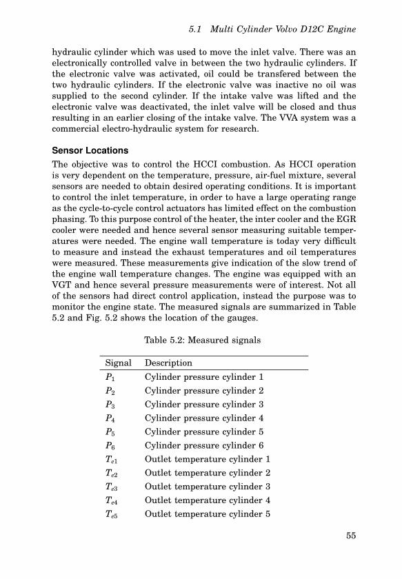
5.1 Multi Cylinder Volvo D12C Engine
hydraulic cylinder which was used to move the inlet valve. There was anelectronically controlled valve in between the two hydraulic cylinders. Ifthe electronic valve was activated, oil could be transfered between thetwo hydraulic cylinders. If the electronic valve was inactive no oil wassupplied to the second cylinder. If the intake valve was lifted and theelectronic valve was deactivated, the inlet valve will be closed and thusresulting in an earlier closing of the intake valve. The VVA system was acommercial electro-hydraulic system for research.
Sensor Locations
The objective was to control the HCCI combustion. As HCCI operationis very dependent on the temperature, pressure, air-fuel mixture, severalsensors are needed to obtain desired operating conditions. It is importantto control the inlet temperature, in order to have a large operating rangeas the cycle-to-cycle control actuators has limited effect on the combustionphasing. To this purpose control of the heater, the inter cooler and the EGRcooler were needed and hence several sensor measuring suitable temper-atures were needed. The engine wall temperature is today very difficultto measure and instead the exhaust temperatures and oil temperatureswere measured. These measurements give indication of the slow trend ofthe engine wall temperature changes. The engine was equipped with anVGT and hence several pressure measurements were of interest. Not allof the sensors had direct control application, instead the purpose was tomonitor the engine state. The measured signals are summarized in Table5.2 and Fig. 5.2 shows the location of the gauges.
Table 5.2: Measured signals
Signal Description
P1 Cylinder pressure cylinder 1
P2 Cylinder pressure cylinder 2
P3 Cylinder pressure cylinder 3
P4 Cylinder pressure cylinder 4
P5 Cylinder pressure cylinder 5
P6 Cylinder pressure cylinder 6
Te1 Outlet temperature cylinder 1
Te2 Outlet temperature cylinder 2
Te3 Outlet temperature cylinder 3
Te4 Outlet temperature cylinder 4
Te5 Outlet temperature cylinder 5
55
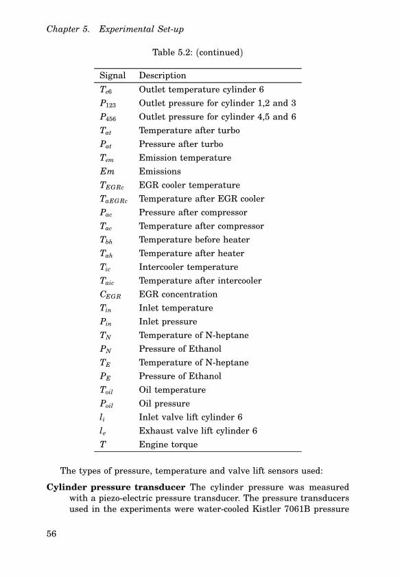
Chapter 5. Experimental Set-up
Table 5.2: (continued)
Signal Description
Te6 Outlet temperature cylinder 6
P123 Outlet pressure for cylinder 1,2 and 3
P456 Outlet pressure for cylinder 4,5 and 6
Tat Temperature after turbo
Pat Pressure after turbo
Tem Emission temperature
Em Emissions
TEGRc EGR cooler temperature
TaEGRc Temperature after EGR cooler
Pac Pressure after compressor
Tac Temperature after compressor
Tbh Temperature before heater
Tah Temperature after heater
Tic Intercooler temperature
Taic Temperature after intercooler
CEGR EGR concentration
Tin Inlet temperature
Pin Inlet pressure
TN Temperature of N-heptane
PN Pressure of Ethanol
TE Temperature of N-heptane
PE Pressure of Ethanol
Toil Oil temperature
Poil Oil pressure
li Inlet valve lift cylinder 6
le Exhaust valve lift cylinder 6
T Engine torque
The types of pressure, temperature and valve lift sensors used:
Cylinder pressure transducer The cylinder pressure was measuredwith a piezo-electric pressure transducer. The pressure transducersused in the experiments were water-cooled Kistler 7061B pressure
56

5.2 Measurement Aspects
transducers. The calibrated pressure range for the transducer was0–250 bar and the natural frequency was 45 kHz [Kistler 7061 B,2004]. The transducers were mounted in a bored pipe, where thetransducers were flush mounted. This is important as otherwise theresonance frequency in the pipe will affect the pressure measure-ments and degrade the resolution of the measurements. An exampleon the pipes length effect on the resolution can be found at p. 480in [Egeland and Gravdahl, 2002].
Pressure transducer The pressure transducers measuring the pressureoutside the cylinders, for placement see Fig. 5.2, were Keller PAA-21S. Two types with different measuring range were used. Rangewas 0-5 bar or 0-10 bar [Keller PAA-21S, 2004]. The pressure trans-ducers measured the absolute pressure.
Temperature sensor Thermocouples of type K from Pentronic were usedin the experiments [Pentronic, 2004]. The Thermocouples measuredthe absolute temperatures.
Engine crank sensor The engine crank encoder was an incrementalencoder from Leine & Lindes [Linde, 2004]. The encoder had theresolution of 1800 pulses per revolution.
Valve lift sensor For measuring the valve lift of the inlet and exhaustvalves, a Hall element was used.
5.2 Measurement Aspects
The signal-to-noise (SNR) ratio gives indication on how much influencesthe noise have on the measurements. The single most important mea-surements are the cylinder pressure which is directly used for estimationof the combustion timing α . In Fig. 2.6, a visual indication on the SNRand its variation for the cylinder pressure is given. The SNR is calculatedusing the energy of the signal, y, and the noise, v.
SN R =eyy
evv
(5.1)
eyy =∑
y(k)y(k) (5.2)
evv =∑
v(k)v(k) (5.3)
In Table 5.3 SNR for cylinder pressure, inlet pressure, and inlet tempera-ture at different operating conditions and crank angles, at IVC, TDC andpeak pressure. Notice that even in the case that the engine is natural
57
Chapter 5. Experimental Set-up
Table 5.3 Signal-to-Noise Ratio
Pcyl (1.0 bar) Pcyl (2.4 bar) Pin Pin Tin Tin
Pos. IVC TDC PP IVC TDC PP 1.0bar 2.4bar 45C 100C
SNR 58.8 1.1e5 3.9e5 305 7.4e5 2.5e6 2.9e4 4.1e5 1.4e5 5.0e5
aspirated (1.0 bar) the SNR is 58.8. The combustion starts around TDCand at that point the SNR is 1.1e5 or more. The operational engine speedvaried from 600 to 2000 rpm. Typical maximum engine speed for an heavyduty engine is around 2000 rpm. A sample of the cylinder pressure sen-sor is taken every 0.2 CAD or 5 times for each CAD. Then the samplingfrequency in the case of 2000 rpm is
Fs = 2000 ⋅36060
⋅ 5 = 60kHz (5.4)
Data Acquisition and Control Cards
The used data acquisition and control cards were:
Microstar DAP 5400a/627 The Microstar DAP 5400a/627 is a fast par-allel sampled data acquisition card for real-time application underLinux or Windows. It had 16 analog inputs and 8 separate 1.25MHz AD-converters with 14 bits resolution. The cylinder pressuredata acquisition was controlled by an encoder connected to the crankshaft of the engine. The resolution of the encoder was 1800 pulsesper revolution, resulting in that a cylinder pressure sample wastaken at every encoder pulse, i.e., every 0.2 crank angle degree. Assoon as one cylinder passed EVO, pressure data were transferredfrom the AD card to the main program. The cylinder pressure onlyused six of the channels. The other channels were also used, butthe signals changed through the experiment. The inlet temperatureoften occupied one of the spare channels, resulting in that the inlettemperature was sampled both with the Microstar card and the HPlogger.
HP 3852A The HP logger sampled the various temperatures and pres-sure and the engine torque. The logged data were sent to the mainprogram. The sampling rate of the logger was 0.4 Hz. The loggeractuated the voltage level to the intercooler and the EGR cooler.
NI 6014 The NI 6014 is a multifunction analog, digital, and timing card.In the experiments, it was used to actuate the voltage level for theheater. This was done once per each engine cycle.
58

5.2 Measurement Aspects
Exhaust gas analysis The exhaust gas analysis system was from Booinstrument providing software and system integration. The systemconsisted of: A flame ionization detector from JUM Engineering formeasuring the HC level in the emissions; A chemoluminescence de-tector for of measuring NOx level in the emissions, the detectionprinciple relying on that fact that mixing NO with ozone produces alight-emitting reaction; Three SICK-MAIHAK analyzers were usedto measure the CO, CO2 and O2 level in the emissions. The exhaustgas analysis system was also used to estimate the air/fuel ratio.
Control Architecture
The engine was controlled by combined data acquisition and engine con-trol system. The engine control system ran on a standard PC (Pentium 42.4 GHz) with GNU/Linux operating system. The distribution used wasRed Hat 8. The main program was written in C++. The combustion timingcontroller was designed in Simulink and converted to stand alone C-codeusing the automatic code generation tool of Real Time Workshop. Then,the C-code was compiled to an executable program communicating withthe main program. FIFO pipes1 were used for the communication betweenthe combustion timing controller and the main program. This feature gavea system where controllers were easily implemented and put into oper-ation. The controllers could also be replaced on-line without restart ofthe system. This property saved a lot of time when new controllers weretested. The heater and the two cooler controllers were implemented di-rectly in C++. In order to assure good real-time performance, the datasaving on disk was run as a separate thread with low priority.
All data coming from various sensors around the engine were collectedin the main program (Fig. 5.3). These data included various temperaturesand pressures collected via a data logger, sampling at low sampling rate,various temperatures and cylinder pressures collected via a MicrostarDAP, sampling at fast sampling rate, and exhaust emissions data fromthe emission system sampling at low sampling rate. The program usedfour threads: Main thread, which collected the cylinder pressure and per-form the control; Logger tread, which collected data from the data logger;Emission treads, which collect data from the emission system; Savingtread, which was active when the data were saved. The firing order forthe cylinders was [1 5 3 6 2 4]. An engine cycle is 720 crank angle degreeswith combustion cycle every 120 crank angle degree.
Even if the main program had several threads, the fuel control wassequential and the steps could be summarized as:
1Pipe is an interprocess communication (IPC) method which you can use to link C pro-grams and C++ programs with each other
59

Chapter 5. Experimental Set-up
GUI
Main
Combustion timing control
(Real−Time Workshopgenerated C−code)
PCLinux
Microstar
Emission
DAP5400a/627
HP Logger Fuel/VVAController
Simulink
Figure 5.3 Schematic view of the data acquisition and control system
1. The cylinder pressure data were sampled by a Microstar 5400A/627data acquisition processor. As soon as one cylinder passed ExhaustValve Opening, pressure data were transferred from the AD card tothe main program. As a result, a pressure segment was sent every120 crank angle degree, the segmentations being shown in Fig. 5.4.The pressure segment consists of pressure data for all six cylinders.When six segments were received, the total pressure trace for theengine cycle was received. The segmentation size was chosen as atrade-off between having sufficient cylinder pressure data in orderto be able to do simple heat release calculations as early as possibleand guaranteeing enough time for sampling of cylinder pressure.
2. When a new pressure segment was available in the main program,a simplified rate of heat release calculation was performed on thecylinder next in fire order, where control inputs such as combustiontiming α , peak pressure and pressure gradient were sent to thecombustion timing controller.
3. The combustion time control signal, i.e., the output from the dualfuel or VVA controller, was then sent back to the main programand the fuel injector was programmed with a new fuel setting. Thefuel injection cycle began at the TDC gas exchange point (TDCG E).In order to have true cycle-to-cycle control, the injection durationhad to be determined and programmed prior to TDCG E which wasachieved.
Conditional upon limits for cylinder peak pressure and pressure gradient,the main program had an engine check feature that could cut the fuelinjection immediately.
To summarize, the input variables which could be controlled in the set-up, were the inlet temperature, inlet pressure, engine speed, injected fuel
60

5.3 Single Cylinder Volvo TD100 Engine
−360 −240 −120 0 120 240 3600
1.6
3.2
4.8
6.4
8x 10
6
−360 −240 −120 0 120 240 3600
360
720
1080
1440
1800P
ress
ure
[Pa]
En
ergy
[J]
Crank angle [CAD]
Figure 5.4 A typical pressure and heat release curve with the segmentation (dash-
dotted), pressure curve (solid) and the heat release curve (dashed).
energy, fuel ratio between dual fuels and the effective compression ratiousing VVA. Some of these variables interact. For example, the VGT can beused to change the inlet pressure, but also the temperature affect the inletpressure. By changing the effective compression ratio with VVA also the λvalue was effected. This kind of interactions complicated the control. Thefuel ratio and the total injected fuel energy also interacted, in the sensethat when the total energy was increased, the transient behavior of theλ depended on the fuel ratio. It could move to earlier or later timing. Itdepended on the heat of vaporization value of the mixture. A schematicview of the control structure is shown in Fig 5.5.
5.3 Single Cylinder Volvo TD100 Engine
The engine was a modified turbo-charged Volvo TD100 engine. Originally,the engine was a Diesel engine, but the original injection system wasremoved and replaced by a low-pressure, sequential port fuel injectionsystem. The engine was an in-line six cylinder engine, modified to operate
61

Chapter 5. Experimental Set-up
Heat release
Controller
Heater
Cooler
Injectors
Electrical motor
PD
PD
Torque
Tin
EthanolN-Heptane
R f
Controller VVA Valve timing
HCCI
Engine
α ref
Trefin
Fuel Energyref
Speedref
Speed
Pressure
α
PIC
Σ
Σ
Σ
Figure 5.5 Block diagram of the control structure
on one cylinder. It is operated on cylinder 6, which is the cylinder closest tothe flywheel. The other five cylinders were motored. The engine had two-valve cylinder heads, one inlet port, one exhaust port and the geometricproperties for the engine being summarized in Table 5.4. An encoder wasmounted on the crankshaft sending five pulses per crank angle degree.These pulses were used by the dual fuel injection system to monitor thestart of injection and by the data acquisition system. Engine speed wasgoverned by an electrical motor with the capacity for both braking andmotoring.
Previously, this engine was used in several projects but, then, with another data acquisition system.
Air Management System
The engine was equipped with an inlet air heater and long route EGR.The engine was operated with natural aspiration. Figure 5.6 shows aschematic outline of the engine and the air management system. Theelectrical heater, with a capacity of 10 kW, was controlled by a PI con-troller.
62

5.3 Single Cylinder Volvo TD100 Engine
Table 5.4 Single cylinder engine specifications.
Displaced Volume 1600 cm3
Bore 120.65 mm
Stroke 140 mm
Connecting Rod Length 260 mm
Number of Valves 2
Compression Ratio 15.5:1
Fuel Supply PFI
EngineIso−Octane
N−Heptane
EGR Cooler
Heater
Inlet air Exhaust
Figure 5.6 The Volvo TD100 engine set-up
63

Chapter 5. Experimental Set-up
Figure 5.7 The spacer and the placement of the 7 modified spark plugs and thepressure transducer. The seventh spark plug is the normal center position of a sparkplug in a SI engine.
Dual Fuel Injection System
The engine had a identical dual fuel injection system as the Volvo D12Cengine. The only difference was that Iso-Octane was used instead of Ethanol.
Sensors
Experiments with a conventional spark plug with and without its sideelectrode removed were performed. The spark plug was used as an ionsensor, and it was mounted in the spacer placed between the cylinder headand engine block. The spacer had 6 evenly spaced radial 14mm fittings,which accommodated modified spark plugs (Fig. 5.7). The idea with aspacer was Andreas Vressner’s, Ph.D. student at Division of CombustionEngines, who at the time also ran ion current experiment on the engine.The only modification of the spark plugs was the removal of the sideelectrode. The experiments without the spacer were performed both withstandard spark plugs and with modified spark plugs. Figure 5.8 showsthe principal layout of the measuring system. A DC voltage (U) of 85 Vwas applied across the electrode gap. The ion current was sampled bymeasuring the voltage over a resistance (R) of 100 kΩ, inserted in theelectrical circuit. Since the signal current level was low, in the order ofone µ A or lower, it was amplified before the A/D conversion was made.The amplifier had a gain of 23 and a bandwidth of 330 kHz.
For measuring the cylinder pressure, a pressure transducer was fittedto the engine for control and monitoring (Fig. 5.7). The pressure trans-ducer was of the same type as in the Volvo D12C engine set-up.
Data Acquisition and Control Cards
The same data acquisition and control cards as in the Volvo D12C set-upwas used.
64
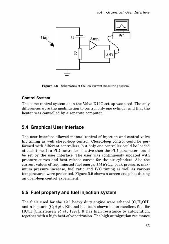
5.4 Graphical User Interface
PC
A/D R
Amp U Gap
Figure 5.8 Schematics of the ion current measuring system.
Control System
The same control system as in the Volvo D12C set-up was used. The onlydifferences were the modification to control only one cylinder and that theheater was controlled by a separate computer.
5.4 Graphical User Interface
The user interface allowed manual control of injection and control valvelift timing as well closed-loop control. Closed-loop control could be per-formed with different controllers, but only one controller could be loadedat each time. If a PID controller is active then the PID-parameters couldbe set by the user interface. The user was continuously updated withpressure curves and heat release curves for the six cylinders. Also thecurrent values of α 50, injected fuel energy, IM EPnet, peak pressure, max-imum pressure increase, fuel ratio and IVC timing as well as varioustemperatures were presented. Figure 5.9 shows a screen snapshot duringan open-loop control experiment.
5.5 Fuel property and fuel injection system
The fuels used for the 12 l heavy duty engine were ethanol (C2H5OH)and n-heptane (C7H16). Ethanol has been shown be an excellent fuel forHCCI [Christensen et al., 1997]. It has high resistance to autoignition,together with a high heat of vaporization. The high autoignition resistance
65
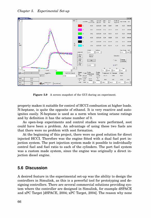
Chapter 5. Experimental Set-up
Figure 5.9 A screen snapshot of the GUI during an experiment.
property makes it suitable for control of HCCI combustion at higher loads.N-heptane, is quite the opposite of ethanol. It is very reactive and auto-ignites easily. N-heptane is used as a norm when testing octane ratingsand by definition it has the octane number of 0.
As open-loop experiments and control studies were performed, sootcould have been a problem. An advantage of using these two fuels arethat there were no problem with soot formation.
At the beginning of this project, there were no good solution for directinjected HCCI. Therefore was the engine fitted with a dual fuel port in-jection system. The port injection system made it possible to individuallycontrol fuel and fuel ratio to each of the cylinders. The port fuel systemwas a custom made system, since the engine was originally a direct in-jection diesel engine.
5.6 Discussion
A desired feature in the experimental set-up was the ability to design thecontrollers in Simulink, as this is a powerful tool for prototyping and de-signing controllers. There are several commercial solutions providing sys-tem where the controller are designed in Simulink, for example dSPACEand xPC Target [dSPACE, 2004; xPC Target, 2004]. The reason why none
66

5.7 Summary and Concluding Remarks
of these solutions were used in the experimental set-up was that none ofthe systems supported data acquisition card with sampling of at least 6channels simultaneous and event-based sampling and possibility to savethe measured data2. Therefore an in-house solution based on Simulinkand Real-Time Workshop for C-code generation of the controllers wereimplemented. The platform used was Linux and it was found that ordi-nary Linux distributions were sufficient to fulfill the time-demands forcycle-to-cycle control, and real-time Linux versions, for example KURT,did not need to be used. The use of standard PC made it possible to havea flexible platform for development of customized control systems, as forexample a wide range of data acquisition cards were accessible. Previ-ously, Windows 95 and Windows XP was used as operating system in allexperiments at the Division of Combustion Engine. The Windows basedsystem had several sample delays in the system and system crashes tookplace.
During a valve lift the valve lift signal saturated in our configurationand only the beginning and ending of the lift could be measured. As theVVA system used was an electro-hydraulic one with a camshaft to lift thevalves, the amplitude of the valve lift will be lower if the timing of IVOor EVO are retarded.
In the experiential set-up the dual-fuel system was more precise inthe actuation that the VVA system. In comparison, the fuel injectors weremore precise in the injected amount of the injected amount of fuel thanthe VVA-system was in achieving a specific IVC crank angle. This wasdue to the mechanic construction of the used VVA system.
The number of sensors used in the experimental set-up are beyondwhat later will be used in production, but for laboratory purpose thesesensors are useful.
5.7 Summary and Concluding Remarks
This chapter has discussed the experimental set-ups used. The set-upshave been designed in order to provide feedbacks for control and to mon-itor the engine system. The proposed control structure using controllersdesigned in Simulink and the possibility to change the controller usedon-line gives an flexible solution suitable for laboratory research.
2This was the situation in the year 2002.
67
6
Candidate Feedback
Sensors
For feedback control of HCCI suitable feedback of the combustion phasingis necessary. As described in Sec. 5.3 the set-up had sensors for both mea-suring cylinder pressure and cylinder ion current. An ion current sensoris less expensive and more environmentally robust, therefore it is inter-esting to compare the combustion phasing information on a HCCI enginefrom the two different sensors. From the pressure measurements thereare several methods to obtain a combustion phasing information. As thefeedback are used on a cycle-to-cycle basis, the method should preferablehave low complexity in order to fulfill the real-time demands. In the sec-ond part of this chapter a comparison of various methods are presented.
6.1 Cylinder Pressure vs Cylinder Ion Current
Currently, cylinder pressure transducers are expensive and have shortlife span. It is therefore interesting to find a cheaper sensor with longdurability. In this section, ion current measurements and pressure mea-surements at HCCI operating points are studied and compared. The ex-periments have been performed on the experimental set-up described inSec. 5.3. All the experiments were performed in open-loop at steady-state.Petter Strandh and Magnus Christensen performed the experiments. Thecontribution of the author, consisted in the analysis of the experiment.In the comparison between α based on cylinder pressure and on ion cur-rent measurements, an experimental set-up with dual fuels and a single-cylinder engine was used, see Sec. 5.3. Pressure-based α calculated viaheat-release is denoted α 50 and α based on ion current is denoted α ion
50 . Wewill show that it is possible to observe a measurement from the ion cur-
68
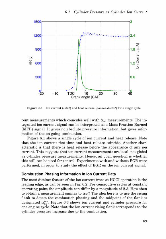
6.1 Cylinder Pressure vs Cylinder Ion Current
−20 −10 TDC 10 20 30 400
300
600
900
1200
1500
HR
[J]
Crank angle [CAD]−20 −10 TDC 10 20 30 40
0
0.6
1.2
1.8
2.4
3
Ion C
urr
ent [µ
A]
Figure 6.1 Ion current (solid) and heat release (dashed-dotted) for a single cycle.
rent measurements which coincides well with α 50 measurements. The in-tegrated ion current signal can be interpreted as a Mass Fraction Burned(MFB) signal. It gives no absolute pressure information, but gives infor-mation of the on-going combustion.
Figure 6.1 shows a single cycle of ion current and heat release. Notethat the ion current rise time and heat release coincide. Another char-acteristic is that there is heat release before the appearance of any ioncurrent. This suggests that ion current measurements are local, not globalas cylinder pressure measurements. Hence, an open question is whetherthis still can be used for control. Experiments with and without EGR wereperformed, in order to study the effect of EGR on the ion current signal.
Combustion Phasing Information in Ion Current Data
The most distinct feature of the ion current trace at HCCI operation is theleading edge, as can be seen in Fig. 6.2. For consecutive cycles at constantoperating point the amplitude can differ by a magnitude of 2-3. How thento obtain a measurement similar to α 50? The idea here is to use the risingflank to detect the combustion phasing and the midpoint of the flank isdesignated α ion
50 . Figure 6.3 shows ion current and cylinder pressure forone engine cycle. Note that the ion current rising flank corresponds to thecylinder pressure increase due to the combustion.
69

Chapter 6. Candidate Feedback Sensors
0 2 4 6 8 10
0
0.5
1
1.5
2
2.5
3
Ion
curr
ent
[µA
]
CAD
Figure 6.2 Ion current from five consecutive cycles. Notice that the cycles has aspread in amplitude. The spread in phasing is correlated to α 50.
0
0.3
0.6
0.9
1.2
1.5
−20 −10 TDC 10 20 30 0
12
24
36
48
60
Ion
curr
ent
Crank angle
Cyl
inde
rpr
essu
re
Pressure and ion current
Figure 6.3 Ion current (solid) and cylinder pressure (dashed).
70

6.1 Cylinder Pressure vs Cylinder Ion Current
0 0.2 0.4 0.6 0.8 110
−3
10−1
0 0.2 0.4 0.6 0.8 110
−5
10−3
10−1
0 0.2 0.4 0.6 0.8 10
0.5
1
−1 0 1 2 3 4 5 6
0
2
4
6
Autospectrum of cylinder pressure
Coherence
Normalized Frequency
Autospectrum of ion current
αio
n50
α p50
Figure 6.4 Autospectrum of α p50 (upper) and α ion
50 (middle). Coherence spectrumbetween α ion
50 and α p50 (middle). Correlation between α ion
50 and α p50. Two cases, ’x’
and ’+’ (lower).
Comparison between Cylinder Pressure and Ion Current
Figure 6.4 shows the correlation between α ion50 and α 50 for two cases, noted
as ’+’ and ’x’. It is well centered along the line representing identity. Bothcases have a correlation coefficient of 0.87. The experiments were carriedout in open loop at constant operating point. The variance of α ion
50 was 0.30for case ’+’ and 0.64 for case ’x’. This can be compared with the varianceof α 50 which was 0.22 for case ’+’ and 0.47 for case ’x’.
71
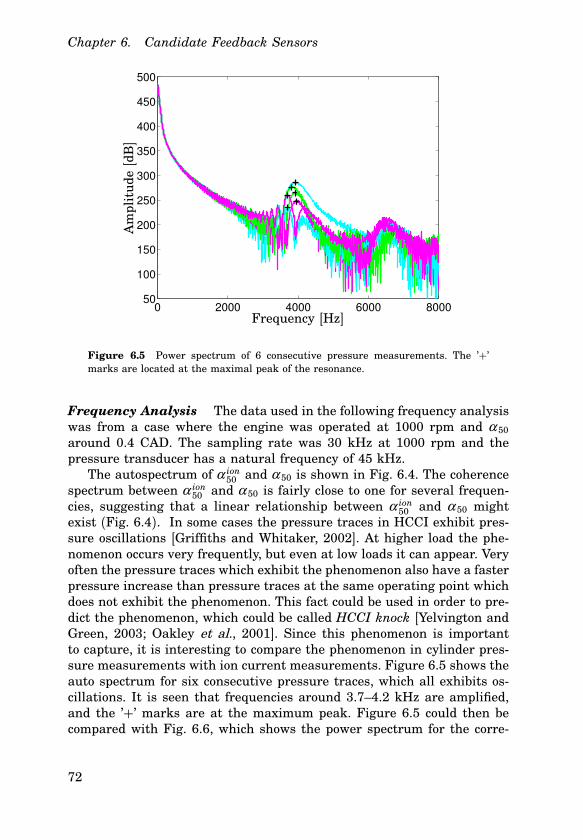
Chapter 6. Candidate Feedback Sensors
0 2000 4000 6000 800050
100
150
200
250
300
350
400
450
500
Frequency [Hz]
Am
plit
ude
[dB
]
Figure 6.5 Power spectrum of 6 consecutive pressure measurements. The ’+’marks are located at the maximal peak of the resonance.
Frequency Analysis The data used in the following frequency analysiswas from a case where the engine was operated at 1000 rpm and α 50
around 0.4 CAD. The sampling rate was 30 kHz at 1000 rpm and thepressure transducer has a natural frequency of 45 kHz.
The autospectrum of α ion50 and α 50 is shown in Fig. 6.4. The coherence
spectrum between α ion50 and α 50 is fairly close to one for several frequen-
cies, suggesting that a linear relationship between α ion50 and α 50 might
exist (Fig. 6.4). In some cases the pressure traces in HCCI exhibit pres-sure oscillations [Griffiths and Whitaker, 2002]. At higher load the phe-nomenon occurs very frequently, but even at low loads it can appear. Veryoften the pressure traces which exhibit the phenomenon also have a fasterpressure increase than pressure traces at the same operating point whichdoes not exhibit the phenomenon. This fact could be used in order to pre-dict the phenomenon, which could be called HCCI knock [Yelvington andGreen, 2003; Oakley et al., 2001]. Since this phenomenon is importantto capture, it is interesting to compare the phenomenon in cylinder pres-sure measurements with ion current measurements. Figure 6.5 shows theauto spectrum for six consecutive pressure traces, which all exhibits os-cillations. It is seen that frequencies around 3.7–4.2 kHz are amplified,and the ’+’ marks are at the maximum peak. Figure 6.5 could then becompared with Fig. 6.6, which shows the power spectrum for the corre-
72
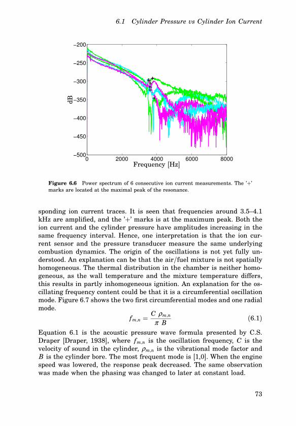
6.1 Cylinder Pressure vs Cylinder Ion Current
0 2000 4000 6000 8000−500
−450
−400
−350
−300
−250
−200
Frequency [Hz]
dB
Figure 6.6 Power spectrum of 6 consecutive ion current measurements. The ’+’marks are located at the maximal peak of the resonance.
sponding ion current traces. It is seen that frequencies around 3.5–4.1kHz are amplified, and the ’+’ marks is at the maximum peak. Both theion current and the cylinder pressure have amplitudes increasing in thesame frequency interval. Hence, one interpretation is that the ion cur-rent sensor and the pressure transducer measure the same underlyingcombustion dynamics. The origin of the oscillations is not yet fully un-derstood. An explanation can be that the air/fuel mixture is not spatiallyhomogeneous. The thermal distribution in the chamber is neither homo-geneous, as the wall temperature and the mixture temperature differs,this results in partly inhomogeneous ignition. An explanation for the os-cillating frequency content could be that it is a circumferential oscillationmode. Figure 6.7 shows the two first circumferential modes and one radialmode.
fm,n =C ρm,n
π B(6.1)
Equation 6.1 is the acoustic pressure wave formula presented by C.S.Draper [Draper, 1938], where fm,n is the oscillation frequency, C is thevelocity of sound in the cylinder, ρm,n is the vibrational mode factor andB is the cylinder bore. The most frequent mode is [1,0]. When the enginespeed was lowered, the response peak decreased. The same observationwas made when the phasing was changed to later at constant load.
73
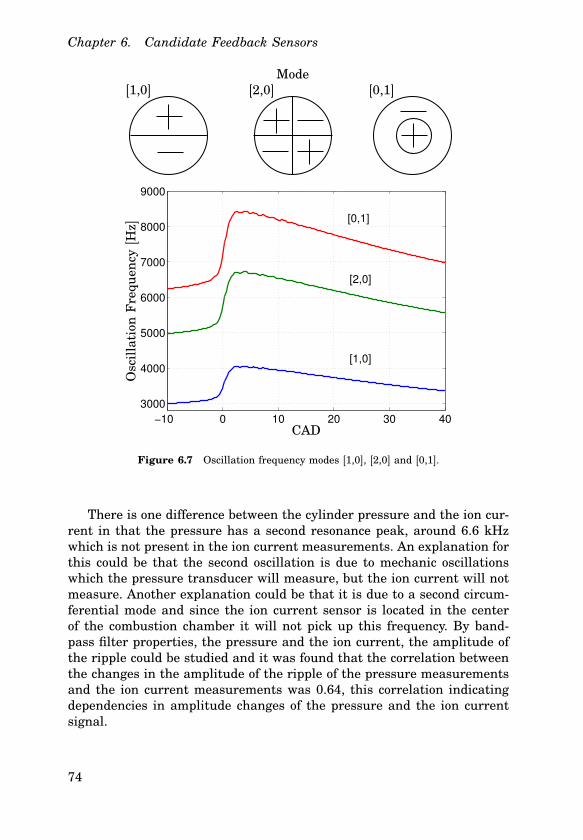
Chapter 6. Candidate Feedback Sensors
CAD [1,0] [2,0] [0,1]Mode
−10 0 10 20 30 40
3000
4000
5000
6000
7000
8000
9000
[0,1]
[2,0]
[1,0]
CAD
Osc
illa
tion
Fre
quen
cy[H
z]
Figure 6.7 Oscillation frequency modes [1,0], [2,0] and [0,1].
There is one difference between the cylinder pressure and the ion cur-rent in that the pressure has a second resonance peak, around 6.6 kHzwhich is not present in the ion current measurements. An explanation forthis could be that the second oscillation is due to mechanic oscillationswhich the pressure transducer will measure, but the ion current will notmeasure. Another explanation could be that it is due to a second circum-ferential mode and since the ion current sensor is located in the centerof the combustion chamber it will not pick up this frequency. By band-pass filter properties, the pressure and the ion current, the amplitude ofthe ripple could be studied and it was found that the correlation betweenthe changes in the amplitude of the ripple of the pressure measurementsand the ion current measurements was 0.64, this correlation indicatingdependencies in amplitude changes of the pressure and the ion currentsignal.
74

6.2 Candidates for combustion phasing feedback
6.2 Candidates for combustion phasing feedback
What signal is best suitable for closed-loop control of an HCCI engine? Thesignal should be accurate, robust and estimated during the combustioncycle, in order to be used for cycle-to-cycle control. As briefly mentioned inSec. 2.4 there are several alternatives. In this section several candidates ofcombustion phasing, α , for feedback control of HCCI engine. The studiedcandidates are
• 50% of heat release, α 50
• 50% of net heat release with fixed κ , α net50
• Maximum heat release rate, α dQmax
• Maximum pressure, α pmax
• Maximum pressure increase by combustion, α p,cmax
• 50% of maximum pressure increase by combustion and compensa-tion of the volume changes, α p,c,v
50
• Rassweiler&Withrow method for 50% mass fraction burned, α M FB50
A common notation for the different α candidates is α method
criterionwhere
superscript defines which signal is used, and subscript defines the criteriafor finding the crank angle. The only discrepancy is α 50, which lacks statedmethod in superscript notation. All candidates are based on the propertythat cylinder pressure is measured. There exists more candidates, forexample α dp
max, but the chosen candidates catch most of the properties ofcylinder pressure based α estimations.
As the combustion is global, the heat release slope is steep and heatrelease is close to symmetric, the crank angle of 50% burned (α 50) repre-senting a robust measure of the phasing of combustion. This also impliesthat other choices of measures like for instance α 20 or α 80 will not have ashigh robustness against noise as α 50, since an error in percentage releasedenergy will correspond to a larger error in crank angle.
In the following study, α 50 from heat release analysis as in Sec. 2.5 isconsidered to be the best measure of the combustion phasing, α , and allthe other alternatives are evaluated in terms of how well they correspondto α 50. The accuracy of α 50 depends on how well the model parameters aretuned and on pressure measurement noise. Hence, tuning was carefullyperformed.
α 50 based on Qhr
The heat release is calculated as described in Sec. 2.5, α 50 then beingestimated by finding the crank angle where half of the energy has been
75

Chapter 6. Candidate Feedback Sensors
released. This is when the bulk of combustion takes place, and the slope ofthe Qhr-curve is steep. This property makes it robust to noise and errorsin the physical constants and is a candidate for the determination of α .
α net50 based on Qnet
hr
α net50 can be found at the crank angle where Qnet
hr reaches half its maximumvalue. Heat release analysis has the drawback that it cannot calculate α 50
until the expansion stroke is finished and it uses several sub-calculations,for example calculation of the heat transfer. Instead of using heat release,net heat release can be used. If κ is well chosen, the maximum value ofQnet
hr is reached before the end of the expansion cycle. The calculationcomplexity is decreased as well, Qnet
hr being given by
dQnethr
dθ=
κ
κ − 1p
dV
dθ+
1κ − 1
Vdp
dθ(6.2)
where a constant κ is used. If we compare this with the complete heatrelease Eq. (2.11), we notice that the difference is that κ is constantand Qht and Qcr is not taken into account. The quantity Qnet
hr gives agood approximation of α 50 since the slope of the Qnet
hr and Qhr-curves arevery steep and coincides. Also Qnet
hr is calculated by integration. In orderto perform a fast α determination, without using the complete cylinderpressure trace, for online cycle-to-cycle feedback control the κ value inthe Qnet
hr calculation was set to a lower value than the expected physicalκ . The lower κ assures an early and robust detection of α , since the Qnet
hr
has an early global maximum, caused by the negative slope in the Qnethr
curve.
α dQmax based on maximum Qhr rate
The crank angle of the maximum heat release rate, dQmaxhr , can also be
used as an estimation of α , but it has the drawback of being more noisesensitive. The benefit is that it provides a fast estimate as it only requirespressure measurements until the maximal slope has been reached.
α pmax based on maximum pressure
The crank angle of the maximum pressure, pmax, during the cycle—alsocalled location of peak pressure (LPP)— can be used as an estimation ofα , based on the assumption that the crank angle where the pressure hasits maximum is in the vicinity of the middle of the combustion since thecombustion rate if fast. This is a rough estimate, but it has the benefit ofnot needing any calculations or calibrations. Using the crank angle of pmax
as an estimation of α fulfills our requirements on fast calculation. How-ever, this approach only works when there is a global maximum pressure
76
6.2 Candidates for combustion phasing feedback
due to combustion. In cases of combustion before TDC or late combustionwhere the peak pressure is at TDC, α p
max therefore fails to give an es-timate of α . Since the HCCI combustion is governed by the state of theengine, it is vital to have a robust feedback signal. α p
max gives the sameα for a cycle which misfired and for one cycle which had very late com-bustion. A misfired cycle resulting in lower engine temperature and inunburned exhaust gases. But a very late combustion will only decreasethe engine temperature slightly and result in none or only a small amountof unburned exhaust gases. The difference between these two cases, havelarge impact on the next cycle. Therefore, α p
max is not a accurate or robustmeasurement of α . Another drawback is that α p
max is closely tied to thecombustion volume and it would, if used as feedback of α , pull the esti-mate towards TDC. This results in a poor estimate in the vicinity of TDCwhere knocking combustion is likely to occur.
α p,cmax based on maximum pressure increase due to combustion
One method of achieving a more robust estimate is to subtract the mo-tored pressure from the measured pressure. Then, the new pressure curverepresents the increased pressure due to combustion, pc. This would givea global maximum even for late combustions and for combustion beforeTDC. Based on the assumption that the maximal pressure for this newpressure curve is in the vicinity of the middle of the combustion for highcombustion rates, α could then be found.
α p,c,v50 based on pressure increase due to combustion
As α pmax and α p,c
max fail to give a good indication of α , the following ap-proach is suggested: Find the crank angle where pressure increase due tocombustion has reached half its maximum level when compensating forthe volume change, α p,c,v
50 . α p,c50 is when not compensating for the volume
change. The volume compensation is achieved by multiplying the pres-sure trace due to combustion with the volume change. This results in anestimation of α with similar properties as α 50. The slope of the pressurecurve is at α p,c,v
50 steep. The benefits with this method are several. Sinceonly pressure trace is used, it is not necessary to have absolute pressure,instead relative pressure is sufficient. The cylinder pressure transducersonly measure relative pressure and for heat release calculation the offsetmust be calculated. Also there is no need in calibration of parameters. Inthe heat release calculations, several parameters are needed to be tuned,such as the parameters in the heat transfer equations. It can be calcu-lated before the engine cycle is finished and can be used for cycle-to-cyclecontrol. Finally, it also has low complexity.
α p,c,v50 is one measurement of the combustion phasing, whereas also
other levels could be interesting. It could be that the pressure increase
77
Chapter 6. Candidate Feedback Sensors
should reach a certain level, absolute or percentage of the maximum. theselevel could also be changed for different operating conditions. Since anHCCI engine has cycle-to-cycle variations, models of the pressure increasecould be used to design model predictive control of this pressure level, inorder to assure that the pressure increase starts at the right CAD.
α M FB50 based on MFB estimation
The Rassweiler and Withrow method is a well established method for es-timating the mass fraction burned, MFB [Rassweiler and Withrow, 1938].The method decomposes the actual change in cylinder pressure, from onepressure sample to the next, into the change in pressure which wouldresult if no combustion were taking place (polytropic process) and an ad-ditional change which is the result of combustion. It is then assumedthat the increase in MFB is proportional to the change in pressure fromcombustion. Thus, for pressure sample i,
(∆pc)i = pi − pi−1
(Vi−1
Vi
)κ
where ∆pc is the increase in cylinder pressure due to combustion and κ(constant) is the polytropic exponent, MFB can now be computed as
mb(i)
mb(total)=
∑ij=0 ∆(pc) j
∑Nj=0 ∆(pc) j
where it is assumed that sample 0 is between inlet valve closing and thestart of combustion, and that sample N is after combustion has finished.The method has limitations, heat transfer effects are included only to theextent that the polytropic exponent κ differs appropriately from γ . In thelimit when the crank angle step ∆θ → 0 , the difference equation for ∆pc
becomes a differential equation. This differential equation can be derivedstarting from the differential form of a polytropic process
d(pvVκ ) = 0
which can be rewritten as
Vκ dpv + κ pvVκ −1dV = 0
Thus, the polytropic pressure differential can be written as
dpv = −κp
VdV
78

6.3 Comparison of combustion phasing candidates
The pressure differential caused by combustion can now be expressed asthe difference between the actual pressure differential and the polytropicpressure differential
dpc = dp −(
−κp
VdV
)= dp + κ
p
VdV .
The expression for dpc can be compared to dQ from a net heat releasecalculation which is
dQnethr =
1γ − 1
V dp +γ
γ − 1pdV =
cv
RV dp +
cp
RpdV
=cv
RV
(dp +
cp
cv
p
VdV
)=
cv
RV
(dp + γ
p
VdV
)=
cv
RV dpc
(6.3)
If κ is assumed to be equal to γ . Thus,
dpc =R
cvVdQnet
hr (6.4)
which is a somewhat distorted version of the net heat release. The fasterthe combustion and the closer to TDC ( dV
dθ small), the smaller the distor-tion, since the volume then becomes closer to constant over the calculationinterval. It does not have the benefit of being fast either since it needsmeasurements for the whole cycle. Thus, it can be improved by using thevalue of mb(total) from the last cycle in the calculation. Then, α M FB
50 canbe estimated the median is reached. This approximation is valid only ifthe operating point changes little from cycle to cycle.
6.3 Comparison of combustion phasing candidates
In the comparison of the different candidates of α , four different cases ofcombustion have been used (Fig. 6.8).
• Case 1 has a global pressure maximum due to combustion (normalcase).
• Case 2 has a local pressure maximum due to combustion.
• Case 3 has increased pressure due to combustion but lacks localmaximum.
• Case 4 has combustion before TDC.
79

Chapter 6. Candidate Feedback Sensors
1
Pre
ssu
re[P
a]
-30 -20 -10 0 10 20 30 40 50
2
3
4
5
6
6
7
8x 10 Cases
-30 -20 -10 10 20 30 40 50
0
0
500
1000
1500
Qh
r[J
]
Qn
eth
r[J
]
-30 -20 -10 10 20 30 40 50
0
0
500
1000
1500
-30
-20
-20 -10
0
0 10
20
20 30
40
40 50
80
60
100
dQ
hr
[J/C
AD
]
Pre
ssu
re[P
a]
CAD []-30 -20 -100 0 10 20 30 40 50
0.5
1
1.5
2
2.5
3
3.56x 10
1
-30 -20 -10
0
0 10 20 30 40 50
0.2
0.4
0.6
0.8
MF
B
CAD []
α α 50 α net50 α dQ
max α pmax α p,c
max α p,c,v50 α M FB
50
Case 1 4.2 4.0 4.0 7.4 9.0 4.2 4.6
Case 2 11.0 10.8 10.0 0.2 16.2 10.4 11.0
Case 3 11.6 11.8 10.6 0.2 18.0 10.8 11.6
Case 4 -2.8 -3.0 -2.4 1.0 3.0 -2.6 -2.6
Figure 6.8 Cylinder pressure traces for different combustion cases(Upper left).Case 1: Global maximum due to combustion (dash-dotted). Case 2: Local maximumdue to combustion (solid). Case 3: No local maximum due to combustion (dashed).Case 4: Combustion before TDC (dotted). The other figures show Qhr , Qnet
hr , dQhr ,pc, MFB for the 4 cases. The ‘*’ marks the CAD for the estimated α -values. Thesquare marks the α p,c,v
50 -value. The table shows the α for the different cases andcandidates.
80

6.3 Comparison of combustion phasing candidates
Table 6.1 Correlation and standard deviation (std) information for the four stud-ied cases expressed in crank angle degree. The residual, e, is the error between α 50and the other α candidates.
α candidates α 50 α net50 α dQ
max α p,cmax α p
max α p,c,v50 α M FB
50
Corr. to α 50 1.000 0.998 0.713 0.801 0.835 0.997 0.943
Std of α (1) 0.396 0.395 0.503 0.641 0.449 0.376 0.382
Std of e (1) 0.000 0.109 0.411 0.505 0.577 0.121 0.118
Std of α (2&3) 0.829 0.809 8.114 1.054 3.594 0.825 0.813
Std of e (2&3) 0.000 0.232 7.892 0.751 4.163 0.262 0.273
Std of α (4) 0.226 0.214 0.370 0.516 0.366 0.237 0.226
Std of e (4) 0.000 0.094 0.330 0.627 0.351 0.098 0.089
In Fig. 6.8, Qhr, Qnethr , dQhr, pc, MFB and their estimates of α are
shown for the four different cases. In case 1, α pmax and α p,c,v
max gives lateestimation of α and α p
max but fails completely to estimate of α in cases 2and 3. What also can be noted is that α p,c,v
50 gives similar indication of α asα 50, but tends to give an earlier indication in the late combustion cases.In Fig. 6.9, the different candidates of α are shown for several cycles. Inorder to better visualize the trends, the figure shows both low-pass filteredα and non-filtered α . From the non-filtered α it can be observed that theyall have similar high frequency properties. From the low-pass filtered α itcan observed that α 50, α net
50 , α p,c,v50 and α M FB
50 give very similar α -value. Butα p
max and α pvmax give late α -values, not near the actual combustion phasing.
α dQmax tends to give too early α -values. Also α p,c
50 has this problem, but α p,c,v50
where the volume changes are taken into account give an estimate thatis close to α 50. It can be noticed that the difference between α 50 andα p,c,v
50 becomes larger when the combustion phasing moves toward latecombustion.
As previously mentioned α 50 is assumed to be the best possible esti-mate of α . Therefore, it is interesting to study coherence between α 50 andthe other candidates (Fig. 6.10). In Table 6.1 the correlation between α 50
and the other α candidates are presented. α net50 , α M FB and α p,c,v
50 gives high-est coherence spectrum, close to one. The table also presents the varianceof α and the residuals, e, where the residuals are the difference betweenα 50 the other α candidates. We note that α dQ
max and α pmax have high vari-
ance in Case 4. In the case of late combustion α dQmax is noise sensitive
since only partial combustion occurs, which makes the variance of the αestimate large.
81
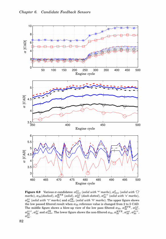
Chapter 6. Candidate Feedback Sensors
50 100 150 200 250 300 350 400 450 5000
2
4
6
8
10
350 400 450 5003.5
4
4.5
5
460 465 470 475 480 485 490 495 500
3
3.5
4
4.5
5
5.5
6
α[C
AD
]α
[CA
D]
α[C
AD
]
Engine cycle
Engine cycle
Engine cycle
Figure 6.9 Various α -candidates: α p,cmax (solid with ‘*’ marks), α p
max (solid with ‘’
marks), α 50(dashed), α M FB50 (solid), α net
50 (dash-dotted), α p,c,v50 (solid with ‘+’ marks),
α p,c50 (solid with ‘O’ marks) and α dQ
max (solid with ‘’ marks). The upper figure showsthe low passed filtered result when α 50 reference value is changed from 2 to 5 CAD.The middle figure shows a blow-up view of the low pass filtered α 50, α M FB
50 , α net50 ,
α p,c,v50 , α p,c
50 and α dQmax. The lower figure shows the non-filtered α 50, α M FB
50 , α net50 , α p,c,v
50 ,α p,c
50 .
82
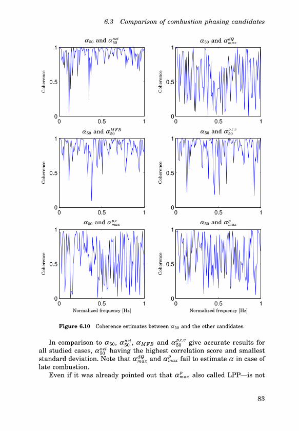
6.3 Comparison of combustion phasing candidates
0 0.5 10
0.5
1
0 0.5 10
0.5
1
0 0.5 10
0.5
1
0 0.5 10
0.5
1
0 0.5 10
0.5
1
0 0.5 10
0.5
1
Normalized frequency [Hz]Normalized frequency [Hz]
α 50 and α net50 α 50 and α dQ
max
α 50 and α p,c,v50
α 50 and α p,cmax α 50 and α p
max
α 50 and α M FB50
Coh
eren
ce
Coh
eren
ceC
oher
ence
Coh
eren
ceC
oher
ence
Coh
eren
ce
Figure 6.10 Coherence estimates between α 50 and the other candidates.
In comparison to α 50, α net50 , α M FB and α p,c,v
50 give accurate results forall studied cases, α net
50 having the highest correlation score and smalleststandard deviation. Note that α dQ
max and α pmax fail to estimate α in case of
late combustion.Even if it was already pointed out that α p
max also called LPP—is not
83

Chapter 6. Candidate Feedback Sensors
−10 −5 0 5 10 15 202
4
6
8x 10
6
−10 −5 0 5 10 15 20−1000
0
1000
2000
P[P
a]
Hea
tre
leas
e[J
]
CAD [degree]
Figure 6.11 Pressure traces and heat release curves at different load conditions:1700 J (4 Bar IMEP) (solid), 1500 J (3.4 Bar IMEP) (dashed) and 1000 J (1.8 BarIMEP) (dash-dotted). In the upper figure, ’+’ marks the location of α p
max and in thelower figure, ’+’ marks the location of α net
50 .
a robust measurement of the combustion phasing, a more detailed studyshows the problem. In Figs. 6.11 and 6.12, the cylinder pressure curvesand the corresponding heat release are shown for three different loadcases; 1000 J, 1500 J and 1700 J. It can be observed that α p
max and α net50
give different indication of α . It can also be observed that the combustionduration differ, but it is strongly dependent on the λ value. Since α p
max
gives an indication when almost all fuel have been burned, the combustionduration have significant effect on α . In the experiments the engine speed,inlet temperature and fuel ratio were kept constant, only the total amountof injected fuel was varied. It was found that the distributions betweenthe two measurements were similar, but there are statistical offsets (Fig.6.13). The bias between α p
max and α net50 are: for the 1000 J load case less
than a half CAD; for the 1500 J load case approximately 2 CAD; for the1700 J load case approximately 2.5 CAD. It can also be noted that theα p
max is not significantly affected by the load change. The 1000 J load casealso includes three cycles where the combustion occurred so late that themaximum pressure was at top dead center, which also can be seen in Fig.6.13. Due to all these properties that α p
max has, it seems to be far fromthe best feedback alternative in order to control HCCI. But thereby itcan not be concluded that it can not successfully be used. In production,cost-effective sensors are essential and α p
max might provide sufficiently
84
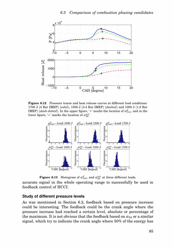
6.3 Comparison of combustion phasing candidates
−10 −5 0 5 10 15 202
4
6
8x 10
6
−10 −5 0 5 10 15 20−1000
0
1000
2000
P[P
a]
Hea
tre
leas
e[J
]
CAD [degree]
Figure 6.12 Pressure traces and heat release curves at different load conditions:1700 J (4 Bar IMEP) (solid), 1500 J (3.4 Bar IMEP) (dashed) and 1000 J (1.8 BarIMEP) (dash-dotted). In the upper figure, ’+’ marks the location of α p
max and in thelower figure, ’+’ marks the location of α net
50 .
2 4 6 8 10 120
10
20
30
2 4 6 8 10 120
10
20
30
2 4 6 8 10 120
10
20
30
2 4 6 8 10 120
10
20
30
2 4 6 8 10 120
10
20
30
2 4 6 8 10 120
10
20
30
α pmax—Load 1000 J α p
max—Load 1500 J α pmax—Load 1700 J
α net50 —Load 1000 J α net
50 —Load 1500 J α net50 —Load 1700 J
Occ
urr
ence
sO
ccu
rren
ces
Occ
urr
ence
sO
ccu
rren
ces
Occ
urr
ence
sO
ccu
rren
ces
CAD [degree] CAD [degree] CAD [degree]
Figure 6.13 Histogram of α pmax and α net
50 at three different loads.
accurate signal in the whole operating range to successfully be used infeedback control of HCCI.
Study of different pressure levels
As was mentioned in Section 6.2, feedback based on pressure increasecould be interesting. The feedback could be the crank angle where thepressure increase had reached a certain level, absolute or percentage ofthe maximum. It is not obvious that the feedback based on α 50 or a similarsignal, which try to indicate the crank angle where 50% of the energy has
85
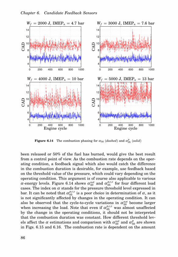
Chapter 6. Candidate Feedback Sensors
0 200 400 600 800 1000
4
6
8
10
12
14
0 200 400 600 800 1000
4
6
8
10
12
14
0 200 400 600 800 1000
4
6
8
10
12
14
0 200 400 600 800 1000
4
6
8
10
12
14
CA
D
CA
D
CA
D
CA
DWf = 2000 J, IMEPn = 4.7 bar Wf = 3000 J, IMEPn = 7.6 bar
Wf = 4000 J, IMEPn = 10 bar Wf = 5000 J, IMEPn = 13 bar
Engine cycle Engine cycle
Figure 6.14 The combustion phasing for α 50 (dashed) and α p05 (solid)
been released or 50% of the fuel has burned, would give the best resultfrom a control point of view. As the combustion rate depends on the oper-ating condition, a feedback signal which also would catch the differencein the combustion duration is desirable, for example, use feedback basedon the threshold value of the pressure, which could vary depending on theoperating condition. This argument is of course also applicable to variousα -energy levels. Figure 6.14 shows α net
50 and α p,c,v05 for four different load
cases. The index on α stands for the pressure threshold level expressed inbar. It can be noted that α p,c,v
05 is a poor choice in determination of α , as itis not significantly affected by changes in the operating condition. It canalso be observed that the cycle-to-cycle variations in α net
50 become largerwhen increasing the load. Note that even if α p,c,v
05 was almost unaffectedby the change in the operating conditions, it should not be interpretedthat the combustion duration was constant. How different threshold lev-els affect the α estimations and comparison with α net
50 and α p50 are shown
in Figs. 6.15 and 6.16. The combustion rate is dependent on the amount
86
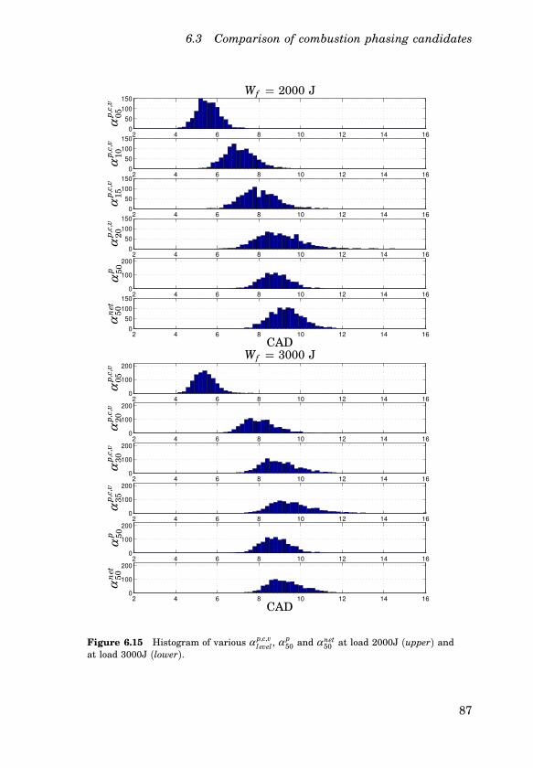
6.3 Comparison of combustion phasing candidates
2 4 6 8 10 12 14 160
50
100
150
2 4 6 8 10 12 14 160
50
100
150
2 4 6 8 10 12 14 160
50
100
150
2 4 6 8 10 12 14 160
50
100
150
2 4 6 8 10 12 14 160
100
200
2 4 6 8 10 12 14 160
50
100
150
CAD
αp
,c,v
05α
p,c
,v10
αp
,c,v
15α
p,c
,v20
αp 50
αn
et50
Wf = 2000 J
2 4 6 8 10 12 14 160
100
200
2 4 6 8 10 12 14 160
100
200
2 4 6 8 10 12 14 160
100
200
2 4 6 8 10 12 14 160
100
200
2 4 6 8 10 12 14 160
100
200
2 4 6 8 10 12 14 160
100
200
CAD
αp
,c,v
05α
p,c
,v20
αp
,c,v
30α
p,c
,v35
αp 50
αn
et50
Wf = 3000 J
Figure 6.15 Histogram of various α p,c,vlevel
, α p50 and α net
50 at load 2000J (upper) andat load 3000J (lower).
87

Chapter 6. Candidate Feedback Sensors
2 4 6 8 10 12 14 160
100
200
2 4 6 8 10 12 14 160
100
200
2 4 6 8 10 12 14 160
100
200
2 4 6 8 10 12 14 160
100
200
2 4 6 8 10 12 14 160
100
200
2 4 6 8 10 12 14 160
100
200
αp
,c,v
05α
p,c
,v20
αp
,c,v
40α
p,c
,v50
αp 50
α50
Wf = 4000 J
CAD
2 4 6 8 10 12 14 16 180
100
200
2 4 6 8 10 12 14 16 180
100
200
2 4 6 8 10 12 14 16 180
100
200
2 4 6 8 10 12 14 16 180
100
200
2 4 6 8 10 12 14 160
100
200
2 4 6 8 10 12 14 16 180
100
200
αp
,c,v
05α
p,c
,v20
αp
,c,v
30α
p,c
,v40
αp 50
α50
Wf = 5000 J
CAD
Figure 6.16 Histogram of various α p,c,vlevel
, α p50 and α net
50 at load 4000J (upper) andat load 5000J (lower).
88

6.3 Comparison of combustion phasing candidates
0 2 4 6 8 10 12 140
1
2
3
4
5
6
7
8
9
10x 10
6
CAD
α 4k05
α 3k05
α 2k05
α 50
α p,c,v20
α p50
α p,c,v30
α 50
α p50
α p,c,v20
α 50
α p,c,v40
α p50
Pre
ssu
re[P
a]
Figure 6.17 Combustion rates at various loads, when the inlet pressure and inlettemperature are constant. The thick lines correspond to the pressure due to com-bustion, when the load is 2000J (dashed), 3000J (dash-dotted) and 5000J (solid).The thick lines are mean value curves of 500 cycles. The thin lines are tangentstaken at the point stated in the figure. The indices 2k, 3k and 4k correspond to thethree load cases.
of fuel. The combustion rate at various loads, when the inlet pressure isconstant, can be seen in Fig. 6.17. Note that as the load increases, thecombustion rate increases.
Effects of low resolution and low engine sampling rate
As resolution of the pressure transducers and sampling rates in produc-tion systems is not as high as in our experimental set-up, it is interestingto study how well the best candidates for α perform when the resolution ofthe cylinder pressure transducer is low and the sample rate is low. In Fig.6.18, the result of α 50, α net
50 and α M FB50 where the cylinder pressure has 6
bits resolution and a full engine cycle consists of 240 samples for Case 1,resulting in a sampling interval of 3 CAD. This is to be compared withthe normal 14 bits resolution and 3600 samples for a full engine cycle. Inorder to increase the accuracy of the estimation of α linear interpolationof the cylinder pressure trace was used. In the experiments, the α 50 waschanged from 4 to 6 CAD. The correlation and standard deviation of α for
89

Chapter 6. Candidate Feedback Sensors
50 100 150 200 250 300 350 400 450 5001
2
3
4
5
6
350 400 450 5004
4.5
5
α[C
AD
]α
[CA
D]
Engine cycle
Figure 6.18 Different α -candidates when using low resolution and low samplingrate: α 50 (dash-dotted), α net
50 (solid with ‘’ marks), α p,c,v50 (solid with ‘O’ marks,
α M FB50 (dashed). These could be compared with α 50 when using the resolution and
sampling rate that normally was used in the experimental setup (solid). The signalsare filtered in order to better visual the differences. The lower figure is a closer viewof the engine cycles 350 to 450.
Table 6.2 α candidates when the pressure trace has low resolution and sampledwith low sampling rate. Correlation between α 50 with high resolution and highsampling rate. Standard deviation (std) information for the various α estimate,expressed in CAD. The residual is the error between α 50 with high resolution andhigh sampling rate and the other candidates.
α candidates α 50 α net50 α p,c,v
50 α M FB50
Correlation 0.9921 0.8818 0.9967 0.9879
Std of α (Case 1) 1.563 1.611 1.589 1.562
Std of residual (Case 1) 0.189 0.186 0.173 0.157
in this low resolution and low sampling rate case are presented in Table6.2. Even this low resolution and low samples rate case, α based on α 50,α net
50 , α p,v,c50 and α M FB
50 are fairly accurate. The standard deviation has in-creased in comparison to our normal experimental set-up conditions, butit still suggests that α based on low resolution sensors and low samplingrate can be used for feedback control.
90

6.3 Comparison of combustion phasing candidates
Discussion
In Sec. 6.1 it was observed that when the engine speed was lowered, theresponse peak decreased. The same observation was also made when laterphasing was chosen at constant load. The observation, that the resonancepeak becomes less significant when later phasing at constant load couldbe due to that the effective volume is larger. The larger volume resultingin that the pressure rise will not become as large as in cases of earlyphasing.
The clearcut relationship between cylinder pressure and ion currentmeasurement suggests that one measurement may be reconstructed fromthe other for instance by means of a Kalman filter or some other full-orderobserver.
Apparently, cylinder pressure measurements provide a more robustα estimation than ion current measurements and in this experimentalset-up, the upper limit of λ-value (relative air/fuel ratio) seems to be2.7 for a reliable ion current signal. At higher λ-values, the noise levelcorrupts the measurements. The rich limit for HCCI operation withoutEGR is λ=2. Questions not yet fully addressed are what is the limit ofoperating conditions, and whether the ion current measurements couldreplace pressure sensors in a production-like environment. It was foundthat the placement of the ion current sensor has influence on the ioncurrent signal and a more detailed study was performed in [Vressneret al., 2004].
An ion current signal is local, therefore was measurements with amodified spark plug without a side electrode performed in order to studyif a more global measurement could be achieved [Strandh et al., 2003]Both the ‘standard’ and the ‘modified’ spark plug cases were found togive reliable combustion information. However, the ion current signal wasfound to be higher in the ‘modified’ spark plug case. It seems likely thatthe modified spark plug provides a somewhat less local measurement dueto less shielding by the side electrode.
Estimations of α based on maximum pressure α pmax and α p,c,v
max give alater combustion phasing, which can be explained by the fact that even ifthe combustion duration is short, it still has a duration of few to severalCAD and the maximum pressure is reached near the end of the combus-tion. The fact that the combustion is not symmetric could be because thatthe combustion having a tail due to after-oxidation which might also influ-ence the maximum pressure phasing. Another drawback is that the max-imum pressure estimate is sensitive to noise and fails to indicate whenthe combustion occurs, particularly in the most important cases of latecombustion or early. The estimates α 50, α net
50 , α p,c,v50 and α M FB
50 give sim-ilar results, whereas α dQ
max gives different results. The reason that α dQmax
91
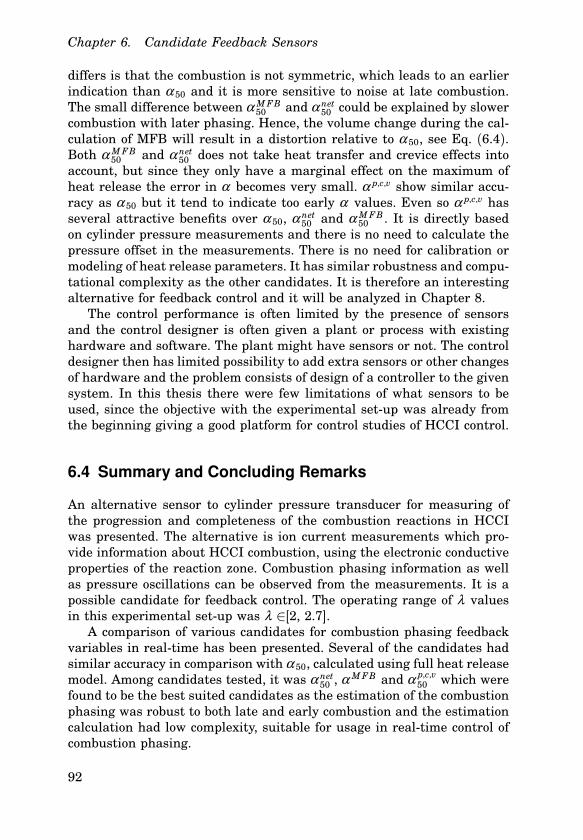
Chapter 6. Candidate Feedback Sensors
differs is that the combustion is not symmetric, which leads to an earlierindication than α 50 and it is more sensitive to noise at late combustion.The small difference between α M FB
50 and α net50 could be explained by slower
combustion with later phasing. Hence, the volume change during the cal-culation of MFB will result in a distortion relative to α 50, see Eq. (6.4).Both α M FB
50 and α net50 does not take heat transfer and crevice effects into
account, but since they only have a marginal effect on the maximum ofheat release the error in α becomes very small. α p,c,v show similar accu-racy as α 50 but it tend to indicate too early α values. Even so α p,c,v hasseveral attractive benefits over α 50, α net
50 and α M FB50 . It is directly based
on cylinder pressure measurements and there is no need to calculate thepressure offset in the measurements. There is no need for calibration ormodeling of heat release parameters. It has similar robustness and compu-tational complexity as the other candidates. It is therefore an interestingalternative for feedback control and it will be analyzed in Chapter 8.
The control performance is often limited by the presence of sensorsand the control designer is often given a plant or process with existinghardware and software. The plant might have sensors or not. The controldesigner then has limited possibility to add extra sensors or other changesof hardware and the problem consists of design of a controller to the givensystem. In this thesis there were few limitations of what sensors to beused, since the objective with the experimental set-up was already fromthe beginning giving a good platform for control studies of HCCI control.
6.4 Summary and Concluding Remarks
An alternative sensor to cylinder pressure transducer for measuring ofthe progression and completeness of the combustion reactions in HCCIwas presented. The alternative is ion current measurements which pro-vide information about HCCI combustion, using the electronic conductiveproperties of the reaction zone. Combustion phasing information as wellas pressure oscillations can be observed from the measurements. It is apossible candidate for feedback control. The operating range of λ valuesin this experimental set-up was λ ∈[2, 2.7].
A comparison of various candidates for combustion phasing feedbackvariables in real-time has been presented. Several of the candidates hadsimilar accuracy in comparison with α 50, calculated using full heat releasemodel. Among candidates tested, it was α net
50 , α M FB and α p,c,v50 which were
found to be the best suited candidates as the estimation of the combustionphasing was robust to both late and early combustion and the estimationcalculation had low complexity, suitable for usage in real-time control ofcombustion phasing.
92

7
Identification of HCCI
Engine Dynamics
In order to understand HCCI engine dynamics and to design controllers,system identification is a key tool. Moreover, the combustion phasing con-trol design requires appropriate models and system output variables forfeedback design. As the engine set-up had two different actuators for thecycle-to-cycle control of the combustion phasing, dual-fuel and VVA, sys-tem dynamic models for each of them will be estimated in the first partof this chapter. In the second part of this chapter, dynamic models of thecylinder pressure trace and the ion current trace, and combustion phasingbased on ion current trace will be estimated.
7.1 Model Variables
An HCCI engine is a complex multiple-input, multiple-output, MIMO,system with interacting inputs and output. The most important problemto solve is the control of the combustion phasing, as this stabilizes thecombustion, effects the performance in load changes and affects the ex-haust emissions. Fast response in load changes is necessary for car andtruck end-users, but perhaps less important if the engine is to be used asa power generator. As the combustion phasing is the most critical and dif-ficult to control, the engine models can be simplified to a multiple-input,single-output, MISO, system, where the combustion phasing α is the out-put. There are many variables which affect α and only some of themare directly controllable, for example the inlet temperature is controllablewhile the wall temperature is a result of previous combustions. Since thecontrol objective is the purpose of the modeling, it is natural to use allthe available control signals, specified in Sec. 5.2 for our experimentalset-up, and model their influence on the combustion phasing. Also other
93

Chapter 7. Identification of HCCI Engine Dynamics
signals could be interesting to use in the identification, such as exhausttemperature and oil temperature. Currently, the cylinder wall tempera-ture is difficult to measure and our experimental set-up lacks a cylinderwall temperature sensor. Instead, the exhaust temperature and the oiltemperature could be used to obtain information about the wall temper-ature. The available inputs in our experimental set-up were described inSec. 5.1.
The main objective of the identification was to obtain models suitablefor control design, in this case combustion phasing control. Hence, themodels should be able to describe the behavior of the combustion phas-ing. For this objective there are two approaches: to estimate models wherecombustion phasing is the output or to estimate models where the pres-sure trace is the output, and then calculate the combustion phasing fromthe trace using some of the methods suggested in Sec. 6.2. The secondmethod is an indirect method for obtaining the combustion phasing. Theadvantage with this method is that more than α can be estimated, forexample the temperature. This makes the model suitable for simulations.
Among the good candidates for α presented in section 6.2, α 50 basedon pressure trace was chosen as the time where the combustion occurred.
Methods and Model Structures
Several methods for estimating dynamic models and model representa-tions exist, each having their benefits and drawbacks [Johansson, 1993].The methods and linear model structures used in this thesis were
Difference Equation Models
ARMAX The ARMAX models (AutoRegressive Moving Average witheXogeneous input) have the following structure
A(z−1)y(k) = z−d B(z−1)u(k) + C(z−1)e(k) (7.1)
where d is a time delay and A, B, C are polynomials.
PEM The PEM models (Prediction Error Method) have the followingmodel structure
A(z−1)y(k) = z−d B(z−1)
F(z−1)u(k) +
C(z−1)
D(z−1)e(k) (7.2)
where d is a time delay and A, B, C, D, F are polynomials. The modelis written as a difference equation. It is the prediction error estimate ofa general linear model, where also a different denominator for the inputand noise can be chosen.
94
7.1 Model Variables
State-Space Models
The estimated models are on state-space form
x(k + 1) = Ax(k) + Bu(k) (7.3)
y(k) = Cx(k) + Du(k) (7.4)
Subspace-based Identification There are several subspace-based meth-ods for identification of state-space models. Among the most well knownare the the multi-variable output-error state-space model algorithm, MOESP[Verhaegen, 1994], and the canonical variable algorithm, CVA [Larimore,1990].
Realization based Impulse Response Analysis A realization basedapproach is to identify a state-space realization of this linear system byusing realization based algorithms [Ho and Kalman, 1966], [Juang andPappa, 1985].
Realization based Step Response Analysis The following step re-sponse analysis (proposed by Rolf Johansson) is a further extension of theimpulse response algorithm. The method is based on the use of Markovparameters Hk, the coefficient matrices of the step response data yk
Nk=1.
The method works by, for suitable r, s such that k+ r + s ≤ N where N isthe number of data points, arranging the Markov parameters in a Hankelmatrix structure
H(k)r,s =
yk+1 yk+2 . . . yk+s
yk+2 yk+3 . . . yk+s+1...
......
. . .
yk+r yk+r+1... yk+r+s−1
(7.5)
and then computing the singular value decomposition (SVD) of
H(0)r,s − H(1)
r,s = UΣV T (7.6)
The impulse response algorithm proposed in [Ho and Kalman, 1966] isused to determine a balanced realization with one input, p outputs, anda system of order n modified to be
xk+1 = Anxn + Bnuk (7.7)
yk = Cnxk + Duk (7.8)
95

Chapter 7. Identification of HCCI Engine Dynamics
where
An = Σ−1/2n UT
n (H(1)r,s − H(2)
r,s )VnΣ−1/2n (7.9)
Bn = Σ−1/2n V T
n Eu (7.10)
Cn = ETy UnΣ−1/2
n (7.11)
D = 0 (7.12)
ETy = [Ipp 0p(r−1)p] (7.13)
ETu = [1 01(s−1)] (7.14)
Σn = diagσ 1,σ 2, ...,σ n (7.15)
Un = matrix of first n columns of U (7.16)
Vn = matrix of first n columns of V (7.17)
Two different implementations of the MOESP algorithm were used,the N4SID-script in the System Identification (SI) Toolbox version 5.0 forMATLAB and the SMI Toolbox for MATLAB [Haverkamp and Verhaegen,1997]. One observation regarding the cylinder pressure or the cylinder ioncurrent is that it has features of an impulse response of a linear system.The idea to interpret the pressure trace as a result of an impulse wassuggested in [Tunestål, 2001], but not exploited. What is most interestingto model in the traces is the ignition delay and the pressure increase dueto combustion, since from this α can be estimated. The duration of thecombustion is significant and a new approach is to interpret the trace asa result of a step response. Even if there would be simultaneous ignition,the duration of combustion is several crank angle degrees as the kineticsare time dependent.
In the model selection procedure and the validation of the models stan-dard methods from system identification has been used. In the first selec-tion of model order, the singular values of the Hankel matrix, the valueof Akaike Final Prediction Error (FPE), the loss function (V ), Variance-Accounted-For (VAF)
VAF = 100 (1 −var(y − y)
var(y))
and the percentage of the output variation that is explained by the model(FIT)
FIT = 100 (1 −hh y − yhh
hhy − yhh)
were used. The loss function is equal to the determinant of the estimatedcovariance matrix of the noise source. In the validation stage, residual
96

7.2 Experiments with Dual Fuel
analysis, autocorrelation and cross validation were performed for all theestimated models. Data trends were eliminated before the identificationprocedure started if not otherwise stated.
7.2 Experiments with Dual Fuel
One of the goals of HCCI engine design, is that an HCCI engine shouldhave similar operation range as a Diesel engine. Hence, models describingthe dynamic behavior of the whole operation range are needed. The objec-tive was to find models where the cycle-to-cycle control signal of the HCCIengine dynamics was the fuel ratio between two fuels, R f . Experiments ina wide range of operating conditions were performed in order to study theeffect of R f , injected fuel energy Wf , inlet temperature Tin, inlet pressurePin, and engine speed n, on α . Also, to some extent the effect of EGR andthe change of VGT on α have been studied. Since the engine is not stableand since too fast combustion at high load could damage the pressuretransducers or the engine, only low-load experiment were carried out inopen loop. Higher load experiments were performed in closed loop.
In the open loop experiments, R f , Wf , Tin and n were excited. TheR f , Wf , Tin were excited by a pseudo-random binary sequence (PRBS)signal and n was excited manually. In the close loop experiments alsoa PRBS signal was added on the reference value of the α . During theclosed loop experiment, the controller was tuned in a conservative setting.Each of the experiments consisted of 2500 or more engine cycles, whichseemed to be sufficient for the identification methods. All the experimentswere run several times in order to supply data for both identification andvalidation. When the experiments started, the engine temperature was atthe operating point.
Naturally Aspirated Experiments
In these experiment the VGT was tuned to low boost pressure.
Experiment 1 This experiment was performed in open-loop at low loadand the VGT was tuned to low boost pressure. The pressure Pin variedbetween 1.05 − 1.3 bar. R f varied between 0.43 − 0.63 (RON 76 − 86), Wf
varied between 1000 − 1500 J/cycle (FuelMEP 5 − 7.5 bar), Tinlet variedbetween 89 − 101C and n varied between 750 − 1500 rpm. A Wf around1000 J/cycle corresponds to running the engine at idle speed, withouttransmitting power, and Wf around 1500 J/cycle corresponds to runningthe engine on a load just above idle. IMEPn varied between 1.5 − 3.5 bar.
97
Chapter 7. Identification of HCCI Engine Dynamics
Experiment 2 This experiment was performed in closed-loop and theVGT was tuned to low boost pressure. The pressure Pin varied between1.1−1.35 bar. Wf varied between 2000−2300 J/cycle (FuelMep 10−11.5bar). In this experiment air/fuel ratio, λ , was close to 2.6, which is nearthe limit of possible operation point for HCCI. The reference value for αwas kept constant at 11 CAD. A PRBS signal was added on the referencesignal with an amplitude of 2 CAD. On the resulting control signal, R f , aPRBS signal was added with an amplitude of 0.4. The Tin varied between68 − 77C and n varied between n = 750 − 1500 rpm. IMEPn variedbetween 5 − 6 bar.
Boost Experiments
In these experiments the VGT was tuned to boost pressure.
Experiment 3 This experiment was performed in open-loop and theVGT was tuned to boost pressure. The pressure Pin was at 1.3 bar. R f
varied between 0.5 − 0.9, Wf was constant at 2000 J/cycle (FuelMEP 10bar), Tinlet was constant at 70C and n was constant at 1000 rpm. IMEPn
was around 4.5 bar.
Experiment 4 This experiment was performed in open-loop and theVGT was tuned to boost pressure. The pressure Pin varied between 1.25−1.55 bar. R f varied between 0.5 − 0.9, Wf varied between 1600 − 2000J/cycle (FuelMEP 8 − 10 bar), Tinlet varied between 70 − 80C and n
varied between 900 − 1200 rpm. IMEPn varied between 3 − 4.5 bar.
Experiment 5 This experiment was performed in closed-loop and theVGT was tuned to generate boost pressure. The pressure Pin was 1.5bar. Wf varied between 2000 − 2200 J/cycle (FuelMEP 10 − 11 bar). Thereference value for α was kept constant at 9 CAD. A PRBS signal wasadded on the references signal with an amplitude of 0.6 CAD. On theresulting control signal, R f , a PRBS signal was added with an amplitudeof 0.1. The Tin varied between 63−65C and n varied between n = 1200−1400 rpm. The resulting IMEPn varied between 4 − 4.7 bar.
Experiment 6 This experiment was performed in closed-loop and theVGT was tuned to generate boost pressure. The pressure Pin was 1.8bar. Wf varied between 3000 − 3200 J/cycle (FuelMEP 15 − 16 bar). Thereference value for α was kept constant at 9 CAD. A PRBS signal wasadded on the reference signal with an amplitude of 0.6 CAD. On theresulting control signal, R f , a PRBS signal was added with an amplitudeof 0.1. The Tin varied between 57−59C and n varied between n = 1200−1400 rpm. The resulting IMEPn was between 7 − 7.5 bar.
98

7.3 Combustion Phasing Modeling with Dual Fuel
Experiment 7 This experiment was performed in closed-loop and theVGT was tuned to generate boost pressure. The pressure Pin was 2.1bar. Wf varied between 4000 − 4200 J/cycle (FuelMEP 20 − 21 bar). Thereference value for α was kept constant at 9 CAD. A PRBS signal wasadded on the reference signal with an amplitude of 0.6 CAD. On theresulting control signal, R f , a PRBS signal was added with an amplitudeof 0.1. The Tin varied between 44−46C and n varied between n = 1200−1400 rpm. The resulting IMEPn was between 9.5 − 10 bar.
Experiment 8 This experiment was performed in closed-loop and theVGT was tuned to generate boost pressure. The pressure Pin was 2.4bar. Wf varied between 5000 − 5200 J/cycle (FuelMEP 25 − 26 bar). Thereference value for α was kept constant at 9 CAD. A PRBS signal wasadded on the reference signal with an amplitude of 0.6 CAD. On theresulting control signal, R f , a PRBS signal was added with an amplitudeof 0.1. The Tin varied between 40−42C and n varied between n = 1200−1400 rpm. The resulting IMEPn varied between 11-13 bar.
Experiment 9 This experiment was performed in closed-loop and theVGT was tuned to generate boost pressure. The pressure Pin varied be-tween 1.4 − 2.4 bar. Wf varied between 2000 − 5000 J/cycle (FuelMEP10 − 25 bar). The reference value for α varied between 9 − 11 CAD. APRBS signal was added on the reference signal with an amplitude of 0.6CAD. On the resulting control signal, R f , a PRBS signal was added withan amplitude of 0.1. The Tin varied between 40 − 43C and n varied be-tween n = 1200 − 1400 rpm. The resulting IMEPn varied between 4-12bar.
7.3 Combustion Phasing Modeling with Dual Fuel
Naturally Aspirated Experiment
Experiment 1 In Table 7.1 the FPE, V, VAF, and FIT scores are shownfor the estimated models of second and third order for cylinder one. TheSMI Toolbox does not calculate the FPE or V, instead only the singularvalues of the Hankel matrix were used in the preliminary model order se-lection. M1 is the model using the MOESP algorithm in the N4SID script,M OESPN4SI D and M2 is the model using the SMI Toolbox, M OESPSM I .The PEM model has the lowest FPE and V values, but the difference tothe other methods is not large. M OESPN4SI D and CVAN4SI D gave al-most identical results. M OESPSM I gave the highest VAF and FIT scores,
99
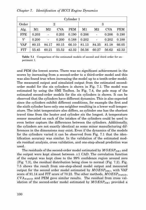
Chapter 7. Identification of HCCI Engine Dynamics
Cylinder 1
Order 2 3
Alg. M1 M2 CVA PEM M1 M2 CVA PEM
FPE 0.203 - 0.203 0.190 0.206 - 0.206 0.190
V 0.200 - 0.200 0.188 0.202 - 0.202 0.188
VAF 80.15 84.17 80.15 66.10 81.13 84.35 81.18 66.05
FIT 55.45 60.21 55.52 42.32 56.56 60.27 56.62 42.32
Table 7.1 Comparison of the estimated models of second and third order for ex-periment 1.
and PEM the lowest scores. There was no significant achievement in thescores by increasing from a second-order to a third-order model and thiswas also found true when increasing the model up to a tenth-order model.The measured output and simulated output from the estimated second-order model for the six cylinders is shown in Fig. 7.1. The model wasestimated by using the SMI Toolbox. In Fig. 7.4, the pole map of theestimated second-order models for the six cylinders is shown. It can beobserved that the cylinders have different dynamics. This is also expectedsince the cylinders exhibit different conditions, for example the first andthe sixth cylinder have only one neighbor resulting in a lower wall temper-ature. The inlet temperature also differs, as cylinder one has the shortesttravel time from the heater and cylinder six the longest. A temperaturesensor mounted on each of the intakes of the cylinders could be used toeven better capture the differences between the cylinders. Additionally,the cylinders are not exactly identical as some minor manufacturing dif-ferences in the dimensions may exist. Even if the dynamics of the modelsfor the cylinders varied it can be observed from Fig. 7.1 that the iden-tification accuracy was similar. In the validation of the estimated mod-els residual analysis, cross validation, and one-step-ahead prediction wasused.
The residuals of the second-order model estimated by M OESPSM I andthe output were kept almost between ±1 CAD. The correlation functionof the output was kept close to the 99% confidence region around zero(Fig. 7.3), the residual distribution being close to normal (Fig. 7.2). Fig.7.5 shows the result from one-step-ahead model output and measuredoutput for the second order model estimated by M OESPSM I , with VAFscore of 91.14 and FIT score of 70.23. The other methods, M OESPN4SI D ,CVAN4SI D and PEM gave similar results. The residual from cross val-idation of the second-order model estimated by M OESPSM I provided a
100
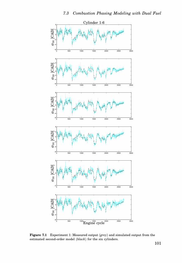
7.3 Combustion Phasing Modeling with Dual Fuel
0 500 1000 1500 2000 2500 3000−6
−4
−2
0
2
4
0 500 1000 1500 2000 2500 3000−6
−4
−2
0
2
4
6
α50
[CA
D]
α50
[CA
D]
Cylinder 1-6
0 500 1000 1500 2000 2500 3000−6
−4
−2
0
2
4
6
0 500 1000 1500 2000 2500 3000−6
−4
−2
0
2
4
α50
[CA
D]
α50
[CA
D]
0 500 1000 1500 2000 2500 3000−5
0
5
0 500 1000 1500 2000 2500 3000−6
−4
−2
0
2
4
α50
[CA
D]
α50
[CA
D]
Engine cycle
Figure 7.1 Experiment 1: Measured output (grey) and simulated output from theestimated second-order model (black) for the six cylinders.
101

Chapter 7. Identification of HCCI Engine Dynamics
−2 −1.5 −1 −0.5 0 0.5 1 1.5 2 2.50
100
200
300
400
Occ
urr
ence
s
Residuals
Figure 7.2 Histogram of the resid-uals of the estimated second-ordermodel.
0 5 10 15 20 25−0.2
0
0.2
0.4
0.6
0.8
1
1.2
0 500 1000 1500 2000 2500−2
−1
0
1
2
3
Correlation function of residual of output α 50
Lag
Res
idu
als
[CA
D]
Engine cycle
Figure 7.3 Residual analysis ofthe estimated second-order model.
−1 −0.5 0 0.5 1−1
−0.8
−0.6
−0.4
−0.2
0
0.2
0.4
0.6
0.8
1
1 2 3 4 5 6
Figure 7.4 Experiment 1: Pole-map of the model for the six cylin-ders. The numbers represent the cor-responding cylinder.
0 50 100 150−1.5
−1
−0.5
0
0.5
1
1.5
2
2.5
α50
[CA
D]
Engine cycle
Figure 7.5 Experiment 1: One-step-ahead prediction model outputof the estimated second-order modelby M OESPSM I (dashed) and mea-sured output (solid).
VAF score of 82.64 and a FIT score of 58.54. Fig 7.6 shows the simula-tion result of the cross validation. The other methods, M OESPN4SI D andCVAN4SI D were close to these values. PEM was significant worse, thedifference being around 10%, in both the VAF and the FIT scores.
Experiment 2
In Table 7.2 FPE, V , VAF, and FIT values are shown of the estimatedmodels of second and third order for cylinder one. Of the estimated mod-
102

7.3 Combustion Phasing Modeling with Dual Fuel
0 500 1000 1500 2000 2500−5
0
5
1500 1600 1700 1800 1900 2000−4
−2
0
2
4
α50
[CA
D]
α50
[CA
D]
Engine cycle
Figure 7.6 Experiment 1: Cross validation of the estimated second-orderM OESPSM I model of cylinder one. Measured α 50 (black) and modeled α 50 (grey).The lower figure shows a closer view of the engine cycle 1500 to 2000.
els, PEM models had the lowest FPE and V values. M OESPN4SI D andCVAN4SI D gave similar results, but has significantly lower VAF and FITscores than M OESPSM I . PEM even failed to give positive values. As forExperiment 1, there was no significant improvements in the scores byincreasing the model order above second order. In Fig. 7.7 the result fromthe estimated second order for cylinder one is shown. The residuals ofthe second-order model estimated by M OESPSM I were less than ±2 CAD.The correlation function of the output was kept inside the 99% confidenceregion around zero. Also in this case, the residuals were found to be nearlynormally distributed. Fig. 7.8 shows the result sequence from one-step-ahead model output for the second-order model estimated by M OESPSM I
and the measured output. The residuals from the cross validation of thesecond-order model estimated by M OESPSM I provided a VAF score of55.6 and a FIT score of 34.3.
Experiment 3 In experiment 3 only the fuel ratio was excited. In thiscase a second-order model gave good a fit. The simulation result of the
103
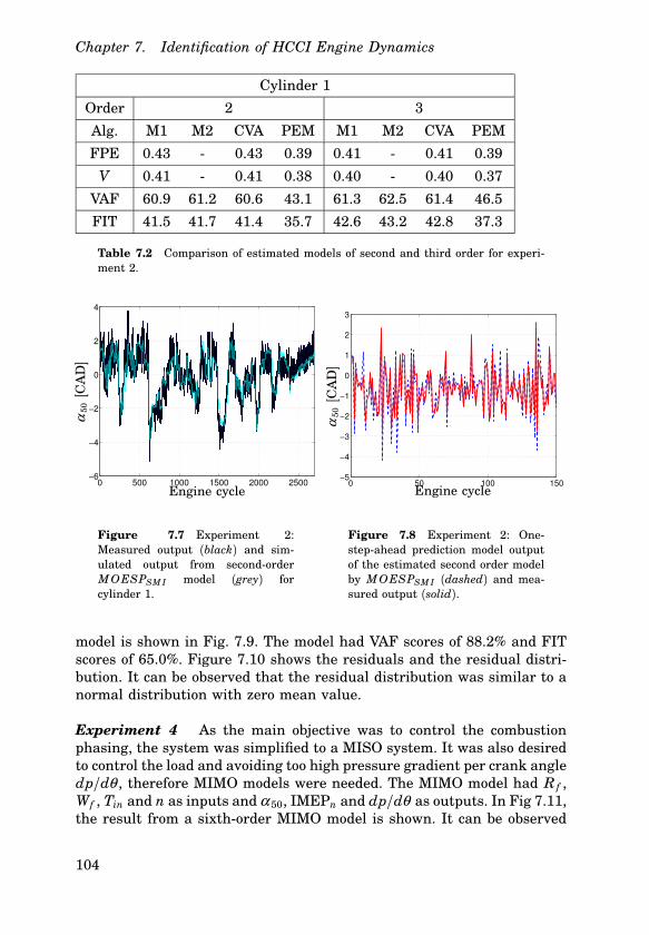
Chapter 7. Identification of HCCI Engine Dynamics
Cylinder 1
Order 2 3
Alg. M1 M2 CVA PEM M1 M2 CVA PEM
FPE 0.43 - 0.43 0.39 0.41 - 0.41 0.39
V 0.41 - 0.41 0.38 0.40 - 0.40 0.37
VAF 60.9 61.2 60.6 43.1 61.3 62.5 61.4 46.5
FIT 41.5 41.7 41.4 35.7 42.6 43.2 42.8 37.3
Table 7.2 Comparison of estimated models of second and third order for experi-ment 2.
0 500 1000 1500 2000 2500−6
−4
−2
0
2
4
α50
[CA
D]
Engine cycle
Figure 7.7 Experiment 2:Measured output (black) and sim-ulated output from second-orderM OESPSM I model (grey) forcylinder 1.
0 50 100 150−5
−4
−3
−2
−1
0
1
2
3
α50
[CA
D]
Engine cycle
Figure 7.8 Experiment 2: One-step-ahead prediction model outputof the estimated second order modelby M OESPSM I (dashed) and mea-sured output (solid).
model is shown in Fig. 7.9. The model had VAF scores of 88.2% and FITscores of 65.0%. Figure 7.10 shows the residuals and the residual distri-bution. It can be observed that the residual distribution was similar to anormal distribution with zero mean value.
Experiment 4 As the main objective was to control the combustionphasing, the system was simplified to a MISO system. It was also desiredto control the load and avoiding too high pressure gradient per crank angledp/dθ , therefore MIMO models were needed. The MIMO model had R f ,Wf , Tin and n as inputs and α 50, IMEPn and dp/dθ as outputs. In Fig 7.11,the result from a sixth-order MIMO model is shown. It can be observed
104

7.3 Combustion Phasing Modeling with Dual Fuel
0 500 1000 1500 2000 2500−3
−2
−1
0
1
2
3
4
0 500 1000 1500 2000 2500
−0.2
−0.1
0
0.1
0.2
Engine cycle
Engine cycle
α50
Rf
Figure 7.9 Upper figure shows measured output (gray) and model output from asecond-order model (black). Lower figure shows the input PRBS signal.
0 500 1000 1500 2000 2500−1.5
−1
−0.5
0
0.5
1
1.5
2
−2 −1.5 −1 −0.5 0 0.5 1 1.5 20
50
100
150
200
250
300
Res
idu
als
Occ
urr
ence
s
Residuals [CAD]
Engine cycle
Figure 7.10 Residuals from the second-order model and the residual distribution.
that the model succeeds in capturing the significant dynamics. The modelhad VAF scores of [86.5% 93.8% 79.2%] and FIT scores of [63.3% 75.1%54.7%]. Figure 7.12 shows the residuals and the residual distribution. Itcan be observed that the residual distribution was similar to the normaldistribution with zero mean value. Figure 7.13 shows cross-validation ofthe estimated sixth-order model. For the cross-validation case, the modelhad VAF scores of [79.8% 87.3% 78.5%] and FIT scores of [55.1% 72.2%52.4%].
105

Chapter 7. Identification of HCCI Engine Dynamics
0 500 1000 1500 2000 2500
−2
0
2
4
0 500 1000 1500 2000 2500
−1
−0.5
0
0.5
1
1.5x 10
5
0 500 1000 1500 2000 2500
−5
0
5
10
15x 10
5
Engine cycle
Engine cycle
Engine cycle
dP
dθ
[Pa/
CA
D]
IME
Pn
[Pa]
α50
[CA
D]
Figure 7.11 Model outputs (thick line black) from the sixth-order MIMO modeland measured outputs (thin grey line).
0 500 1000 1500 2000 2500−2
0
2
4
−2 0 20
200
400
0 500 1000 1500 2000 2500−1
0
1x 10
5
−5 0 5
x 104
0
500
0 500 1000 1500 2000 2500−5
0
5
10x 10
5
−5 0 5
x 105
0
200
400
600
α50
[CA
D]
IME
Pn
[Pa]
dP
dθ
[Pa/
CA
D]
Engine cycle
Engine cycle
Engine cycle α 50 [CAD]
IMEPn [Pa]
dPdθ [Pa/CAD]
Occ
urr
ence
sO
ccu
rren
ces
Occ
urr
ence
s
Figure 7.12 Residuals from the sixth-order MIMO model and the residual distri-bution
106

7.3 Combustion Phasing Modeling with Dual Fuel
0 200 400 600 800 1000 1200 1400 1600 1800 2000 2200−5
0
5
0 200 400 600 800 1000 1200 1400 1600 1800 2000 2200
−1
0
1
x 105
0 200 400 600 800 1000 1200 1400 1600 1800 2000 2200−1
0
1
2x 10
6
α50
[CA
D]
IME
Pn
[Pa]
dp/d
θ[P
a/C
AD
]Engine cycle
Engine cycle
Engine cycle
Figure 7.13 Cross-validation of the sixth-order MIMO model. Model outputs(thick black line) and measured outputs (thin grey line).
Cylinder 1
Order 1 2 3 4 5
FIT 32.9 35.8 35.7 35.7 35.8
VAF 55.4 59.7 59.1 59.3 60.1
Table 7.3 Comparison of estimated models for experiment 5.
Boost Experiment
As it was found that the various subspace algorithms gave similar per-formance, only results using the M OESPN4SI D algorithm are presented.
Experiment 5 In Table 7.3, VAF and FIT values are shown of theestimated models of second- to fifth-order for cylinder one. As for thenaturally aspirated experiments, there were no significant improvementsin the scores by increasing above second order. In Fig. 7.14 the result fromthe estimated second-order model for cylinder one is shown. The singularvalues of the Hankel matrix are shown in Fig. 7.15 and indicating thathigher-order models will probably not increase the model accuracy andthat the noise level is significant. Cross validation gives good results,
107

Chapter 7. Identification of HCCI Engine Dynamics
0 100 200 300 400 500
−2
0
2
0 100 200 300 400 500
−2
0
2
α50
[CA
D]
α50
[CA
D]
Engine cycle
Figure 7.14 Experiment 5: Upper figure shows measured output (solid) and simu-lated output from second-order M OESPSM I model (dashed) for Cylinder 1. Lowerfigure shows cross validation of the second-order M OESPSM I model. Measuredoutput (solid) and model output (dashed).
Cylinder 1
Order 1 2 3 4 5
FIT 29.5 31.8 31.9 32.3 32.5
VAF 50.2 53.1 51.3 51.9 52.2
Table 7.4 Comparison of estimated models of experiment 6.
almost the same VAF and FIT scores as for the identification data set,the VAF score being 52.4 and the FIT score being 30.7.
Experiment 6 In Table 7.4, VAF and FIT values are shown of theestimated models of second to fifth order for cylinder one. As for the nat-urally aspirated experiments, there were no significant improvements inthe scores by increasing above second order. In Fig. 7.16 the result fromthe estimated second order for cylinder one is shown. The singular valuesof the Hankel matrix are shown in Fig. 7.15 indicates that higher-ordermodels will probably not increase the model accuracy and that the noiselevel is significant. It can also be noted that it suggests a third-ordermodel. Cross validation gives good results, with almost the same VAFand FIT scores as for the identification data set, the VAF score being 47.7and the FIT score being 27.5.
108

7.3 Combustion Phasing Modeling with Dual Fuel
0 5 10 152
2.5
3
3.5
0 5 10 152
2.5
3
3.5
0 5 10 152
2.5
3
3.5
0 5 10 152
2.5
3
3.5
log
ofsi
ngu
lar
valu
es
log
ofsi
ngu
lar
valu
es
log
ofsi
ngu
lar
valu
es
log
ofsi
ngu
lar
valu
es
Model orderModel order
Model orderModel order
Experiment 5 Experiment 6
Experiment 7 Experiment 8
Figure 7.15 Singular values of the Hankel matrix used in the model order choicefor experiment 5–8.
0 100 200 300 400 500
−2
0
2
0 100 200 300 400 500
−2
0
2
α50
[CA
D]
α50
[CA
D]
Engine cycle
Figure 7.16 Experiment 6: Upper figure shows measured output (solid) and sim-ulated output from second-order M OESPSM I model (dashed) for cylinder 1. Lowerfigure shows cross validation of the second-order M OESPSM I model. Measuredoutput (solid) and model output (dashed).
Experiment 7 In Table 7.5, VAF and FIT values are shown of theestimated models of second to fifth order for cylinder one. As for the nat-urally aspirated experiments, there were no significant improvements inthe scores of model orders higher than two. In Fig. 7.17 the result from
109
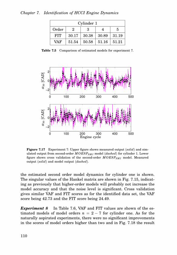
Chapter 7. Identification of HCCI Engine Dynamics
Cylinder 1
Order 2 3 4 5
FIT 30.17 30.38 30.89 31.19
VAF 51.54 50.58 51.16 51.21
Table 7.5 Comparison of estimated models for experiment 7.
0 100 200 300 400 500
−2
0
2
0 100 200 300 400 500
−2
0
2
α50
[CA
D]
α50
[CA
D]
Engine cycle
Figure 7.17 Experiment 7: Upper figure shows measured output (solid) and sim-ulated output from second-order M OESPSM I model (dashed) for cylinder 1. Lowerfigure shows cross validation of the second-order M OESPSM I model. Measuredoutput (solid) and model output (dashed).
the estimated second order model dynamics for cylinder one is shown.The singular values of the Hankel matrix are shown in Fig. 7.15, indicat-ing as previously that higher-order models will probably not increase themodel accuracy and that the noise level is significant. Cross validationgives similar VAF and FIT scores as for the identified data set, the VAFscore being 42.73 and the FIT score being 24.49.
Experiment 8 In Table 7.6, VAF and FIT values are shown of the es-timated models of model orders n = 2 − 7 for cylinder one. As for thenaturally aspirated experiments, there were no significant improvementsin the scores of model orders higher than two and in Fig. 7.18 the result
110

7.3 Combustion Phasing Modeling with Dual Fuel
Cylinder 1
Order 2 3 4 5 6 7
FIT 17.52 19.85 19.97 20.27 20.45 20.46
VAF 28.03 31.19 31.38 31.89 32.19 32.40
Table 7.6 Comparison of estimated models for experiment 8.
0 100 200 300 400 500
−2
0
2
0 100 200 300 400 500
−2
0
2
α50
[CA
D]
α50
[CA
D]
Engine cycle
Figure 7.18 Experiment 8: Upper figure shows measured output (solid) and sim-ulated output from second-order M OESPSM I model (dashed) for cylinder 1. Lowerfigure shows cross validation of the second-order M OESPSM I model. Measuredoutput (solid) and model output (dashed).
from the estimated second order for cylinder one is shown. The singularvalues of the Hankel matrix are shown in Fig. 7.15 indicating as previ-ously that higher-order models will probably not increase the model ac-curacy and that the noise level is significant. Cross validation gave goodresults, as the residual distribution being close to normal with zero meanand similar VAF and FIT scores as for the identified data set, the VAFscore being 25.8 and the FIT score being 16.1.
Experiment 9 In Table 7.7, VAF and FIT values are shown of the es-timated models of model orders n = 2 − 7 for cylinder one. As for thenaturally aspirated experiments, there were no significant improvementsin the scores of model orders higher than three and in Fig. 7.19 the resultfrom the estimated third-order model for cylinder one is shown. Cross
111

Chapter 7. Identification of HCCI Engine Dynamics
Cylinder 1
Order 2 3 4 5 6 7
FIT 17.2 22.0 24.5 24.8 25.9 25.5
VAF 31.9 39.1 42.9 44.3 45.6 45.3
Table 7.7 Comparison of estimated models for experiment 9.
0 100 200 300 400 500 600 700
−4
−2
0
2
4
6
8
0 100 200 300 400 500 600 700
−4
−2
0
2
4
6
8
α50
[CA
D]
α50
[CA
D]
Engine cycle
Figure 7.19 Experiment 9: Upper figure shows measured output (solid) and sim-ulated output from third-order M OESPSM I model (dashed) for cylinder 1. Lowerfigure shows cross validation of the third-order M OESPSM I model. Measured out-put (solid) and model output (dashed).
validation gave good results, as the residual distribution being close tonormal with zero mean and similar VAF and FIT scores as for the iden-tified data set, the VAF score being 37.5 and the FIT score being 20.7.In this experiment the amplitude of the cycle-to-cycle variations were
changed. The variance increased when the load increased, and the modelfail to well describe the changed cycle-to-cycle variance.
112

7.4 Experiments with VVA
7.4 Experiments with VVA
The objective was to find models of the HCCI engine dynamics when theIVC phasing was used as the cycle-to-cycle control signal. Experimentsin a wide range of operating conditions were performed in order to studythe effect of IVC phasing, injected fuel energy Wf , inlet temperature Tin,inlet pressure Pin, and engine speed n, on α .
Experiment 10
This experiment was performed in open-loop at low load and the VGT wastuned to low boost pressure, Pin varied between 1.04-1.07 bar. IVC variedbetween 525-565 CAD, R f was constant at 0.87 (RON 95), Wf variedbetween 1000 − 1400 J/cycle (FuelMEP 5 − 7 bar), Tinlet varied between102 − 114C and n was constant at 1200 rpm. IMEPn varied between1.5 − 3.5 bar.
Experiment 11
This experiment was performed in open-loop at low load and the VGTwas tuned to low boost pressure, Pin varied between 1.04-1.07 bar. IVCvaried between 555-595 CAD, R f was constant at 0.87 (RON 95), Wf wasconstant at 1200 J/cycle (FuelMEP 6 bar), Tinlet was constant at 110C
and n was constant at 1100 rpm. IMEPn was around 3 bar.
7.5 Combustion Phasing Modeling with VVA
Experiment 10
In Fig. 7.20 the results from a fourth-order model are shown, the FITscore being 53.87%. The model was estimated using the N4SIDM OESP
algorithm in Matlab. This fourth-order models are able to capture most ofthe dynamics, but it can be observed that it has some problem to capturethe low frequency behavior correctly. At some operating conditions thegain of the model is too low, for example at cycle 300-400 in Fig. 7.20 andfor other operating conditions the models gain is too high, see for exampleat cycle 1200-1400 in Fig. 7.20. In the experiment the IVC was varied ina wide range and the results indicate that the relationship between IVCand α 50 is nonlinear. In order to capture the behavior, several piecewiselinear or nonlinear models are needed.
Experiment 11
By changing the IVC crank angle the effective compression ratio is changed,resulting in a cylinder temperature change and a change in α 50. Due to
113

Chapter 7. Identification of HCCI Engine Dynamics
0 200 400 600 800 1000 1200 1400 1600 1800 2000−3
−2
−1
0
1
2
3
4
5
6
7
8
α50
[CA
D]
Engine cycle
Figure 7.20 Experiment 10: Measured output (solid) and simulated output fromfourth-order M OESPSM I model (dashed) for cylinder 1.
the movement of the piston, a change of θ IV C has a nonlinear effect onα 50, Figure 7.21. It can be noted that there are two possibilities to obtainthe same α 50, either by closing the inlet valve during the expansion beforeBDC or during the compression after BDC. This experiment included onlyIVC phasing at or after the BDC.
The static nonlinearity can be estimated as a polynomial of fourthorder. A method to linearize the system was to estimate the inverse of thenonlinearity and add this to the system, see Figure 7.22. The system wasthen approximately linear from u
′to u.
Figure 7.23 shows the result of the compensation of the static nonlin-earity. As the compensation was successful u can be approximated by u
′.
The inverse was obtained using a look-up table.As the nonlinearity could be described by a polynomial of power four, a
method to identify the dynamics is to use inputs up to power four. Figure7.24 shows the inputs and output used in the identification.
114

7.5 Combustion Phasing Modeling with VVA
500 520 540 560 580 600 6200
2
4
6
8
10
12
14
16
18
α50
[CA
D]
θ IV C [CAD]
Figure 7.21 The effect of IVC changes on α 50 at steady-state.
u′
u u α 50
HCCI Engine
Dynamics
Figure 7.22 Compensating for the nonlinear characteristics of IVC control, whereu is θ IV C .
The identified models were obtained in state space representation:
x(k + 1) = Ax(k) + B
u(k)
u2(k)
u3(k)
u4(k)
y(k) = C(x(k) + Du(k)
The experiment were performed in open-loop and at low load. In orderto have persistent excitation, θ IV C was excited by a PRBS signal. In this
115
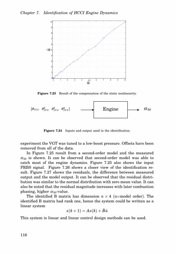
Chapter 7. Identification of HCCI Engine Dynamics
0 1 2 3 4 5 6 7 8 9 100
1
2
3
4
5
6
7
8
9
10
u
u′
Figure 7.23 Result of the compensation of the static nonlinearity.
α 50Engine[θ IV C θ 2IV C θ 3
IV C θ 4IV C]
Figure 7.24 Inputs and output used in the identification.
experiment the VGT was tuned to a low-boost pressure. Offsets have beenremoved from all of the data.
In Figure 7.25 result from a second-order model and the measuredα 50 is shown. It can be observed that second-order model was able tocatch most of the engine dynamics. Figure 7.25 also shows the inputPRBS signal. Figure 7.26 shows a closer view of the identification re-sult. Figure 7.27 shows the residuals, the difference between measuredoutput and the model output. It can be observed that the residual distri-bution was similar to the normal distribution with zero mean value. It canalso be noted that the residual magnitude increases with later combustionphasing, higher α 50-value.
The identified B matrix has dimension n 4 (n=model order). Theidentified B matrix had rank one, hence the system could be written as alinear system
x(k + 1) = Ax(k) + Bu
This system is linear and linear control design methods can be used.
116
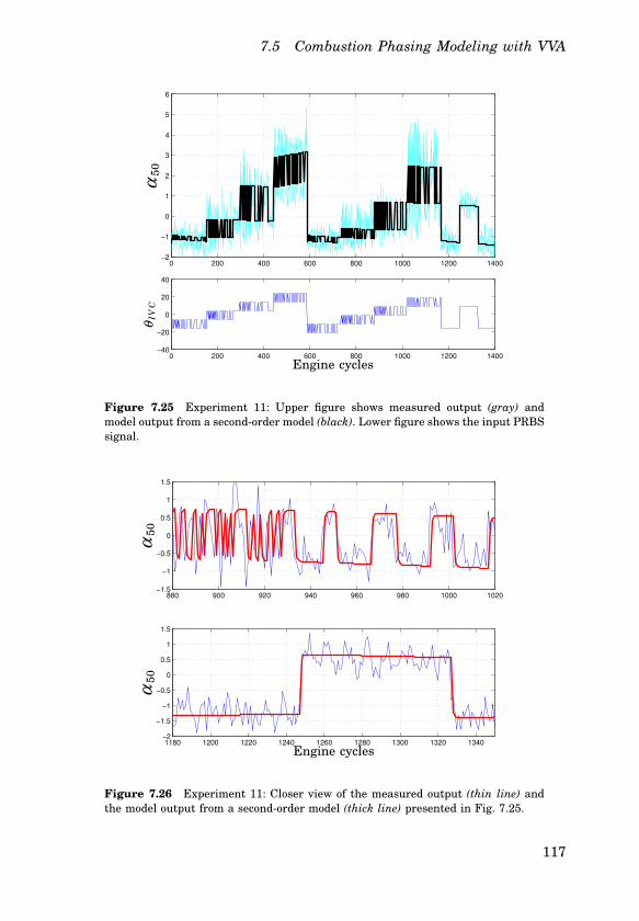
7.5 Combustion Phasing Modeling with VVA
0 200 400 600 800 1000 1200 1400−2
−1
0
1
2
3
4
5
6
0 200 400 600 800 1000 1200 1400−40
−20
0
20
40
α50
θIV
C
Engine cycles
Figure 7.25 Experiment 11: Upper figure shows measured output (gray) andmodel output from a second-order model (black). Lower figure shows the input PRBSsignal.
880 900 920 940 960 980 1000 1020−1.5
−1
−0.5
0
0.5
1
1.5
1180 1200 1220 1240 1260 1280 1300 1320 1340−2
−1.5
−1
−0.5
0
0.5
1
1.5
α50
α50
Engine cycles
Figure 7.26 Experiment 11: Closer view of the measured output (thin line) andthe model output from a second-order model (thick line) presented in Fig. 7.25.
117

Chapter 7. Identification of HCCI Engine Dynamics
0 200 400 600 800 1000 1200 1400−3
−2
−1
0
1
2
3
−3 −2 −1 0 1 2 30
50
100
150
200
250
Residuals
Occ
urr
ence
sO
ccu
rren
ces
Engine cycles
Figure 7.27 Identification residual and its distribution
7.6 Combustion Phasing Effect in Load Changes
Fast changes of the load is a vital property for successful automotiveapplication. A driver wants to have a fast response when pressing theaccelerator. Whereas the load is very dependent on the injected fuel en-ergy, the load can be changed almost instantaneously in our experimentalset-up, at higher loads there is a one cycle delay because the fuel injectorsare not capable of injecting all the fuel before IVC. This problem could besolved by using higher pressure in the injector and hence increasing theinjected volume. What actually limits the change of load is the control ofthe combustion phasing. The combustion phasing needs to be stable, evenat fast load changes. In Fig. 7.28, the injected fuel energy was changedfrom 1000J to 1500J (FuelMEP 5−7.5 bar) resulting in a change of IMEPfrom 2.2 to 4.0 bar. The fuel ratio was kept constant at 0.2 and the inlettemperature was kept constant at 87 C. It can be observed that α isadvanced from approximately 7 to 3.5 CAD. The explanation is that thewall temperature increases and the concentration of fuel increases. The
118
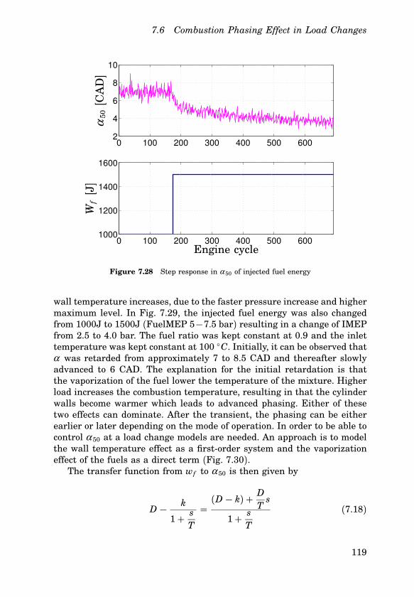
7.6 Combustion Phasing Effect in Load Changes
0 100 200 300 400 500 6002
4
6
8
10
0 100 200 300 400 500 6001000
1200
1400
1600
α50
[CA
D]
Wf
[J]
Engine cycle
Figure 7.28 Step response in α 50 of injected fuel energy
wall temperature increases, due to the faster pressure increase and highermaximum level. In Fig. 7.29, the injected fuel energy was also changedfrom 1000J to 1500J (FuelMEP 5−7.5 bar) resulting in a change of IMEPfrom 2.5 to 4.0 bar. The fuel ratio was kept constant at 0.9 and the inlettemperature was kept constant at 100 C. Initially, it can be observed thatα was retarded from approximately 7 to 8.5 CAD and thereafter slowlyadvanced to 6 CAD. The explanation for the initial retardation is thatthe vaporization of the fuel lower the temperature of the mixture. Higherload increases the combustion temperature, resulting in that the cylinderwalls become warmer which leads to advanced phasing. Either of thesetwo effects can dominate. After the transient, the phasing can be eitherearlier or later depending on the mode of operation. In order to be able tocontrol α 50 at a load change models are needed. An approach is to modelthe wall temperature effect as a first-order system and the vaporizationeffect of the fuels as a direct term (Fig. 7.30).
The transfer function from wf to α 50 is then given by
D −k
1 +s
T
=(D − k) +
D
Ts
1 +s
T
(7.18)
119

Chapter 7. Identification of HCCI Engine Dynamics
0 100 200 300 400 500 6004
6
8
10
0 100 200 300 400 500 6001000
1200
1400
1600
α50
Wf
J
Engine cycle
Figure 7.29 Step response in α 50 of injected fuel energy
wf α 50
D
k
1 +s
T
∑
Figure 7.30 Model of load changes effect on α 50.
The parameters D, k and T vary and depend on the operating conditions.An approach to obtain the parameters are to fit first-order system modelsto the experiments and then use linear regression to obtain the parameterdependency of the operating condition. The idea is that the parametersare a function of wf , ∆wf , R f and α 50. An approach is to use the followingparameterization of D, k and T
D =a1wif + a2∆wf + a3α i
50Rif + a4 (7.19)
k =b1wif + b2∆wf + b3Ri
f + b4α i50 (7.20)
T =c1wif + c2∆wf + c3Ri
f + c4α i50 + c5α i
50Rif (7.21)
where index i indicates the condition when the change of load occur. In
120

7.7 Pressure Trace and Ion Current Trace
0 50 100 150 200 250 300 350 4000
2
4
10−4
10−3
10−2
10−1
100
101
102
10−6
10−4
10−2
10−4
10−3
10−2
10−1
100
101
102
50
100
150
200
α50
[CA
D]
Engine cycle
Normalized frequency
Am
plit
ude
Ph
ase
Figure 7.31 Experiment where the injected fuel energy changes from 1000J to1500J (FuelMEP 5 − 7.5 bar) and where the fuel ratio is 0.5. The upper figureshows experimental data (thin grey), model output from fitted first-order model(thick solid) and model output using the parameters obtained by linear regression(thick dashed). The lower figures show the Bode diagram of the model with theparameters obtained by linear regression.
Figs. 7.31, 7.32 and 7.33 the fitted first-order models and the models withD, k and T parameters obtained from linear regression are shown.
It can be noted that the estimated models capture most of the dynam-ics, and that the dynamic behavior varies significantly depending on thestep size and the operating conditions.
In order to be able to design a feedforward controller it is most vital tocapture the variations of the D-parameter, as the slow change in α 50 dueto changed wall temperature can be stabilized by a feedback controller.The signals wf , ∆wf , R f and α 50 together give an estimation of the enginestate and in Fig. 7.34 the estimation results of D, k and T are shown. Itcan be noted that in all cases the signals wf , ∆wf , R f and α 50 can be usedto give accurate estimations of the parameters. The first-order model andparameter function approach have been validated with cases which werenot used in the estimation of the function parameters, a, b and c (Fig.7.35).
121
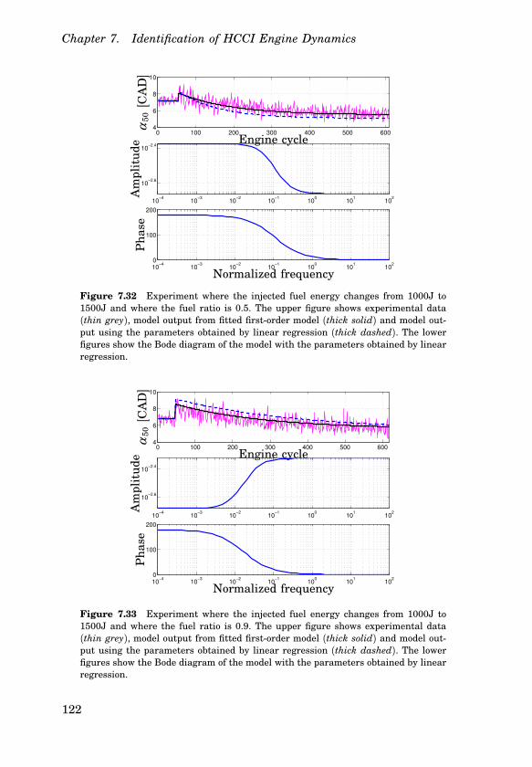
Chapter 7. Identification of HCCI Engine Dynamics
0 100 200 300 400 500 6004
6
8
10
10−4
10−3
10−2
10−1
100
101
102
10−2.6
10−2.4
10−4
10−3
10−2
10−1
100
101
102
0
100
200
α50
[CA
D]
Engine cycle
Normalized frequency
Am
plit
ude
Ph
ase
Figure 7.32 Experiment where the injected fuel energy changes from 1000J to1500J and where the fuel ratio is 0.5. The upper figure shows experimental data(thin grey), model output from fitted first-order model (thick solid) and model out-put using the parameters obtained by linear regression (thick dashed). The lowerfigures show the Bode diagram of the model with the parameters obtained by linearregression.
0 100 200 300 400 500 6004
6
8
10
10−4
10−3
10−2
10−1
100
101
102
10−2.6
10−2.4
10−4
10−3
10−2
10−1
100
101
102
0
100
200
α50
[CA
D]
Engine cycle
Normalized frequency
Ph
ase
Am
plit
ude
Figure 7.33 Experiment where the injected fuel energy changes from 1000J to1500J and where the fuel ratio is 0.9. The upper figure shows experimental data(thin grey), model output from fitted first-order model (thick solid) and model out-put using the parameters obtained by linear regression (thick dashed). The lowerfigures show the Bode diagram of the model with the parameters obtained by linearregression.
122

7.7 Pressure Trace and Ion Current Trace
1 2 3 4 5 6 7 8 9 10 110
0.005
0.01
1 2 3 4 5 6 7 8 9 10 110
0.1
0.2
1 2 3 4 5 6 7 8 9 10 11
0
5
10x 10
−3
Experiment
kD
T
Figure 7.34 Parameter variation of D, k and T . The ’+’ marks is the parame-ters from the fitted first-order model and the ’*’ marks are result from the linearregression.
0 50 100 150 200 250 300 350 400 450 5004
6
8
10
10−4
10−3
10−2
10−1
100
101
102
10−2.56
10−2.47
10−4
10−3
10−2
10−1
100
101
102
0
100
200
α50
[CA
D]
Engine cycle
Normalized frequency
Am
plit
ude
Ph
ase
Figure 7.35 Experiment where the injected fuel energy changes from 1500J to1800J and where the fuel ratio is 0.5. The upper figure shows experimental data(thin grey), model output from fitted first-order model (thick solid) and model out-put using the parameters obtained by linear regression (thick dashed). The lowerfigures show the Bode diagram of the model with the parameters obtained by linearregression.
123

Chapter 7. Identification of HCCI Engine Dynamics
0 20 40 60 80 100
0
2
4
6
x 106
0 5 10 15 20 25 30−0.5
0
0.5
1
1.5
2
2.5Data
Data
Model output
Model output
Error
ErrorIo
ncu
rren
t[µ
A]
Pre
ssu
re[P
a]
CAD
Figure 7.36 Upper figure: Measured pressure (solid) and output a 4th-order statespace model (dashed). Lower figure: Measured ion current (solid) and output a 7thorder state space model (dashed)
7.7 Pressure Trace and Ion Current Trace
In the previous sections, dynamic models of α 50 have been estimated,but it is also possibly to estimate dynamic models of the cylinder pres-sure and ion current trace. One observation regarding the combustion isthat it has features of an impulse response of a linear system. Hence,an approach to identify dynamic models of the increased pressure andion current due to the combustion is to use impulse response analysis. Arealization based-approach is to find a state space realization of this lin-ear system that reproduces the given impulse response [Ho and Kalman,1966]. Figure 7.36 shows a cylinder pressure trace and the impulse re-sponse from an identified fourth-order model starting from TDC. Eventhis low-order model reproduces the pressure trace fairly well. It repro-duces the oscillation and the rise time constant, but it has problems inthe relaxation time constant. Even so the model parameter should con-tain relevant thermodynamical and combustion information. In order toobtain models with similar accuracy of the ion current trace the modelorder needed to be increased. Figure 7.36 shows an ion current trace andthe impulse response from an identified 7:th order model starting from
124

7.7 Pressure Trace and Ion Current Trace
TDC. It is seen that the ion current trace is reproduced quite accuratelyby the identified model, both the oscillation and the time constants.
One way to parameterize the identified model could be to present themas a continuous-time impulse response describing linear system dynamics
y(t) =
∫ t
−∞
h(t − s) u(s)︸︷︷︸=δ (s)
ds = h(t). (7.22)
The identified 4th-order state-space model for the cycle pressure can thebe written as a impulse response:
h(t) = 8.10 ⋅ 106 ⋅ e−0.99t − 3.81 ⋅ 106 ⋅ e−0.85t (7.23)
+ 2.92 ⋅ 1010 ⋅ e−0.73t ⋅ sin(0.67t) + 4.44 ⋅ 106δ (t)
This fourth-order model is one estimation of the pressure, but we have noclaim that it is the best possible model. In this parameterization, the riseand fall time constants and oscillation frequency can easily be found.
Whereas the signals representing ion current and pressure signal areintimately related, they are not identical. A Bode diagram representingthe transfer function from ion current to pressure is given in Fig. 7.37,and in Fig. 7.38 the simulated model output together with measured out-put are presented. The transfer functions were identified by estimatingARMAX models [Johansson, 1993]. It can be observed from Fig. 7.38 thatthe pressure trace can be reconstructed from the ion current signal, evenif the signals differ. The Bode diagrams (Fig. 7.37) of the transfer functionbetween ion current and pressure indicate has a resonant peak at 23 krad/s. In Sec. 6.1 frequency content of cylinder pressure and ion currentshowed that the both measurements had resonant peak at 3.5 − 4.2 kHz.23 k rad/s expressed in Hz is approximately 3.7 kHz which fits well inthe interval of 3.5 − 4.2 kHz. Transforming the estimated discrete modelto continuous-time and written in transfer function form gives
G(s)=B(s)
A(s)
A(s)= s4+1880s3+7.03⋅108s2+5.45⋅1011s +1.06⋅1014
B(s)= 6630s4+1.36⋅109s3+9.23⋅1013s2 +2.07⋅1018s−1.16⋅1021
Modeling of α ion50
Also models which had α ion50 and α net
50 as output were estimated, whichcould directly be used in the control synthesis. The input to the processwas the fuel ratio, R f , and IM EPnet. Removal of offsets and/or trends
125

Chapter 7. Identification of HCCI Engine Dynamics
60
80
100
120
140
160
101
102
103
104
105
−270
−180
−90
0
Mag
nit
ude
[dB
]P
has
e[d
eg]
Frequency [rad/s]
Figure 7.37 Bode diagram of the transfer function between ion current measure-ment without side electrode and pressure. Ion current is input and pressure is theoutput of the 6th-order ARMAX model.
0 5 10 15 20 25 302
4
6
8x 10
6
MeasuredSimulated FIT:92.16%
0 5 10 15 20 25 302
4
6
8x 10
6
MeasuredSimulated FIT:91.73%
0 5 10 15 20 25 302
4
6
8x 10
6
MeasuredSimulated FIT:92.55%
Pre
ssu
re[P
a]P
ress
ure
[Pa]
Pre
ssu
re[P
a]
CAD
Figure 7.38 The simulated model pressure output (dashed) together with mea-sured pressure (solid). The upper figure shows result when using the data used inthe identification, the middle and lower figures show cross-validation results, themodel used being the same as in Fig. 7.37.
126

7.7 Pressure Trace and Ion Current Trace
0 100 200 300 400−4
−3
−2
−1
0
1
2
3
4
0 100 200 300 400−4
−3
−2
−1
0
1
2
3
4
Engine cycleEngine cycle
αio
n50
[CA
D]
αn
et50
[CA
D]
Figure 7.39 Responce in α net50 and α ion
50 to step changes in CA50 reference. Leftfigure: model output from a second order model(grey) and α net
50 (black). Right figure:model output from a second order model (grey) and α ion
50 (black)
were performed before the identification procedure started. Linear modelswere identified by using subspace-based methods [Verhaegen, 1994]. Theidentification results, where VAF and FIT scores, residual analysis andcross validation were performed indicated that lower order models weresufficient. Figure 7.39 shows the simulation results from two identifiedmodels, α net
50 output model and α ion50 output model. Both models were of
second order. Figure 7.40 shows the Bode diagram and Fig. 7.41 shows theNyquist diagram of the second-order models from fuel ratio and IM EPnet
to α ion50 and α net
50 . Both the Bode and the Nyquist diagram indicate asexpected that there are substantial similarities between the models ofα ion
50 and α net50 . The differences are essentially the gain, but also the phase
differs at higher frequency. The phase graph of the model of α ion50 is higher
than Bode diagram phase of the model of α net50 at higher frequencies.
Step Response Analysis
In Fig. 7.42 results from models estimated using step response analysisare shown. The models are of third order and the results indicate thatfor the load cases 1000J to 1500J (FuelMEP 5 − 7.5 bar) a third-ordermodel is sufficient. The most interesting part of the pressure trace tocapture is the part from TDC to the maximum pressure and the modelscapture both the ignition delay and the pressure increase. When the loadincreases, the modeling of the pressure tail becomes poor, and higher-order models are needed in order to capture the pressure tail. The poles
127

Chapter 7. Identification of HCCI Engine Dynamics
102
103
104
50
100
150
200
250
102
103
104
−150
−100
−50
0
50
102
103
104
0
0.2
0.4
0.6
0.8
1
1.2
1.4x 10
−4
102
103
104
−350
−300
−250
−200
−150
−100
−50
0
Input Fuel Ratio Input IMEP
Am
plit
ude
Am
plit
ude
Ph
ase
Ph
ase
Frequency [Hz]Frequency [Hz]
Figure 7.40 Bode diagram (left) showing the transfer function from fuel ratio toα ion
50 (solid) and α net50 (dashed). Bode diagram (right) showing the transfer function
from IMEP to α ion50 (solid) and α net
50 (dashed).
−200 −100 0 100 200 300−200
−150
−100
−50
0
50
100
150
200
−5 0 5 10 15
x 10−5
−8
−6
−4
−2
0
2
4
6
8x 10
−5Input Fuel Ratio Input IMEP
Imag
inar
y
Imag
inar
y
RealReal
Figure 7.41 Nyquist diagram (left) from fuel ratio to α ion50 (solid) and α net
50(dashed). Nyquist diagram (right) showing from IMEP to α ion
50 (solid) and α net50
(dashed).
128

7.7 Pressure Trace and Ion Current Trace
−40 −30 −20 −10 0 10 20 300.5
1
1.5
2
2.5
3
3.5
4
4.5
5x 10
6 Fuel energy = 1000 [J]
CAD
Pre
ssu
re[P
a]
−40 −30 −20 −10 0 10 20 300
1
2
3
4
5
6x 10
6 Fuel energy = 1100 [J]
CAD
Pre
ssu
re[P
a]
−40 −30 −20 −10 0 10 20 300
1
2
3
4
5
6x 10
6 Fuel energy = 1200 [J]
CAD
Pre
ssu
re[P
a]
−40 −30 −20 −10 0 10 20 300
1
2
3
4
5
6
7x 10
6 Fuel energy = 1300 [J]
CAD
Pre
ssu
re[P
a]
−40 −30 −20 −10 0 10 20 300
1
2
3
4
5
6
7x 10
6 Fuel energy = 1400 [J]
CAD
Pre
ssu
re[P
a]
−40 −30 −20 −10 0 10 20 300
1
2
3
4
5
6
7
8x 10
6 Fuel energy = 1500 [J]
CAD
Pre
ssu
re[P
a]
Figure 7.42 Mean pressure traces for different load cases (solid) and model output(dashed).
129
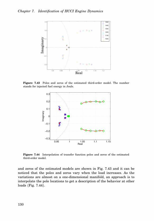
Chapter 7. Identification of HCCI Engine Dynamics
0.9 0.95 1 1.05 1.1 1.15 1.2
−0.2
−0.1
0
0.1
0.2
0.3 1500 1400 1300 1200 1100 1000
Imag
inar
y
Real
Figure 7.43 Poles and zeros of the estimated third-order model. The numberstands for injected fuel energy in Joule.
0.95 1 1.05 1.1 1.15
−0.3
−0.2
−0.1
0
0.1
0.2
0.3
Real
Ima
gin
ary
Figure 7.44 Interpolation of transfer function poles and zeros of the estimatedthird-order model.
and zeros of the estimated models are shown in Fig. 7.43 and it can benoticed that the poles and zeros vary when the load increases. As thevariations are almost on a one-dimensional manifold, an approach is tointerpolate the pole locations to get a description of the behavior at otherloads (Fig. 7.44).
130
7.8 Discussion
7.8 Discussion
Other variables than α 50 were found to describe α also well. These vari-ables may also give the same identification result as the ones with α 50. Allexperiments were carried out when the engine initially was at a steadystate. What yet remains to be done is to model the transient behaviorwhen the engine starts.
The autoignition depends of the cylinder temperature, but in the exper-imental set-up used, neither cylinder temperature or cylinder wall tem-perature were measured. The temperature of the exhaust gas, coolingwater, and the engine oil gave a measurement of the slow trend in thecylinder temperature. Identification results, where these three tempera-tures were added to the already existing inputs and the output was α 50
showed not better result in comparison with the models without thesethree temperatures. These measurements are slow and fails to capturethe transient behavior. In order to have a better estimation of the cylin-der temperature, a cylinder wall temperature sensor may be used. Evenif such measurement is local and do not describe the cylinder head tem-perature, it still may give a better and faster indication of a change inthe cylinder temperature. Hence, may such measurement result in bettermodels of α 50.
Linear models were estimated, but as an HCCI has nonlinear char-acteristics, nonlinear models may improve the result. The VAF and FITscores were used as one among with residual analysis, autocorrelationand cross validation in the evaluation of the models, but only betweenmodels based on the same data set. Both VAF and FIT decreases whenthe cycle-to-cycle variations increases, hence can VAF and FIT not be usedas a measure to qualitatively compare models at which have used datafrom different operation points.
Results from subspace-based methods were presented, but also polyno-mial structures such as NARMAX models were estimated. The identifiedNARMAX models also suggested that lower order models were sufficient.This could be explained by the fact that after estimation of the static non-linearity, the dynamics left are related to temperature, wall and residualgas, which could all be modeled by lower order models.
The reaction kinetics in HCCI combustion are very complex to fullydescribe, even so the identification results indicate that accurate estima-tions models with fuel ratio as input and combustion phasing as outputcan be obtained with lower-order linear models.
131

Chapter 7. Identification of HCCI Engine Dynamics
7.9 Summary and Concluding Remarks
Dynamic models suitable for control design are needed. In this chapter itis shown that system identification methods can successfully be used as atool of obtaining dynamic models of HCCI. Among the methods used therewas found that the state space models gave better result than the differ-ence equation models in modeling of HCCI. In the case of MIMO modelingthe MOESP algorithm in the SMI-toolbox gave significantly better result.The VAF and FIT scores were 40% lower for the two subspace-based al-gorithm in the System Identification Toolbox.
An HCCI engine is not a linear process, but in the range of the ex-periments it was found that lower-order linear dynamic models gave goodaccuracy in modeling of the combustion timing. Identification of modelswere performed in an IMEPn load range of [2, 14] bar. Models of thepressure trace and the ion current trace during combustion have beenestimated and the models of the two feedback options were similar.
132

8
Control of HCCI
Today there exists almost no feedback control of the internal combustionengines in production. The two common types, SI and CI, both have di-rect actuation. The SI engine has some feedback control, since most newengines has knock control and λ control. The motivation for the feedbackcontrol is firstly to avoid damaging the engine and secondly to keep theemissions low. Today, most of the control of the combustion is dependent onhuge engine maps, where all the engine operating points are covered andused for feedforward control. This strategy is not applicable to control ofan HCCI engine, since it is very sensitive to the operating conditions andlacks direct control of the combustion phasing. Additionally, the enginedynamics change and are unstable at some operating points. Therefore,feedback control of the combustion is necessary and pure feedforward can-not solve the problem itself, due to the sensitivity and dynamic propertiesof the HCCI engine.
It has been demonstrated that an HCCI engine can be unstable [Olssonet al., 2002a], and at some operating point the engine was found to bevery sensitive to disturbances. Fig. 8.1 shows an experiment when thepressure gradient reaches the safety limit. At cycle No. 382, the pressuregradient started to grow quickly and at cycle No. 385 the engine was shutdown. The engine was operated in open-loop, and the sudden increase ofthe pressure gradient was probably triggered by excitation. For enginesafety reasons, the maximum allowed pressure gradient per CAD was 40bar/CAD. The experiment shows that feedback control is necessary inorder to control the combustion phasing in an HCCI engine.
The combustion phasing estimates α net50 and α ion
50 were used as feedbackmeasurements for the control. The combustion estimate α net
50 will fromhere on be referred to as α 50 in the text.
133
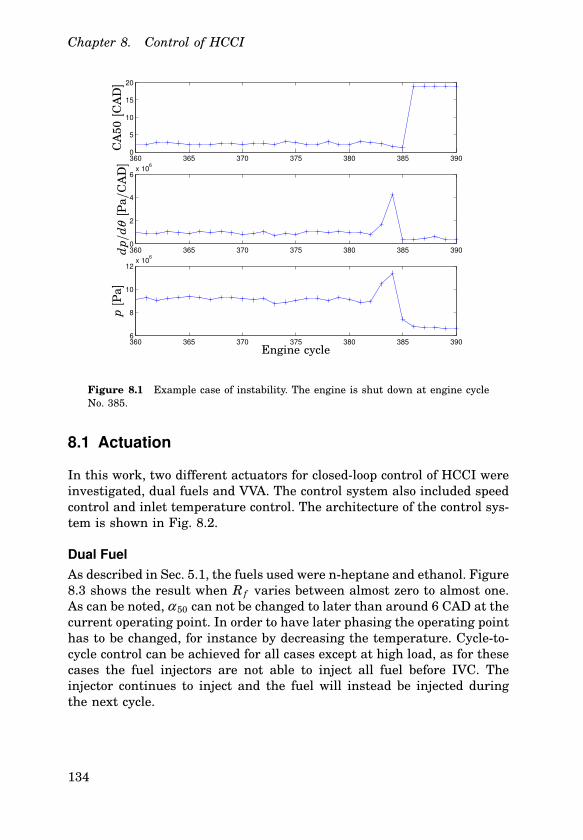
Chapter 8. Control of HCCI
360 365 370 375 380 385 3900
5
10
15
20
360 365 370 375 380 385 3900
2
4
6x 10
6
360 365 370 375 380 385 3906
8
10
12x 10
6
CA
50[C
AD
]d
p/d
θ[P
a/C
AD
]p
[Pa]
Engine cycle
Figure 8.1 Example case of instability. The engine is shut down at engine cycleNo. 385.
8.1 Actuation
In this work, two different actuators for closed-loop control of HCCI wereinvestigated, dual fuels and VVA. The control system also included speedcontrol and inlet temperature control. The architecture of the control sys-tem is shown in Fig. 8.2.
Dual Fuel
As described in Sec. 5.1, the fuels used were n-heptane and ethanol. Figure8.3 shows the result when R f varies between almost zero to almost one.As can be noted, α 50 can not be changed to later than around 6 CAD at thecurrent operating point. In order to have later phasing the operating pointhas to be changed, for instance by decreasing the temperature. Cycle-to-cycle control can be achieved for all cases except at high load, as for thesecases the fuel injectors are not able to inject all fuel before IVC. Theinjector continues to inject and the fuel will instead be injected duringthe next cycle.
134

8.1 Actuation
α 50
Controller
Heater
Cooler
Injectors
Electrical motor
PD
PD
Torque
Tin
Iso-OctaneN-Heptane
R f
Controller VVA Valve timing
HCCI
Engine
α ref
Trefin
Fuel Energyref
Speedref
Speed
p
α ion50
Ion currentPIC
Σ
Σ
Σ
Figure 8.2 The control system.
0 50 100 150 200 250 300 350
2
4
6
8
0 50 100 150 200 250 300 3500
0.2
0.4
0.6
0.8
1
α50
Rf
Engine cycle
Figure 8.3 Combustion phasing when fuel ratio changes. Experiment conditions:Wf = 1400 J (FuelMEP 7 bar), Tin = 95C and Pin = 1.6 bar.
135
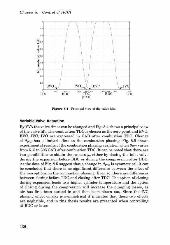
Chapter 8. Control of HCCI
0 100 180 300 360 400 500 540 600 7200
0.1
0.2
0.3
0.4
0.5
0.6
0.7
0.8
0.9
1
TDCTDC BDCBDC TDC[CAD]
EVCEVO IVCIVO
Nor
mal
ized
valv
eL
ift
Figure 8.4 Principal view of the valve lifts.
Variable Valve Actuation
By VVA the valve times can be changed and Fig. 8.4 shows a principal viewof the valve lift. The combustion TDC is chosen as the zero point and EVO,EVC, IVC, IVO are expressed in CAD after combustion TDC. Changeof θ IVC has a limited effect on the combustion phasing. Fig. 8.5 showsexperimental results of the combustion phasing variation when θ IVC variesfrom 515 to 605 CAD after combustion TDC. It can be noted that there aretwo possibilities to obtain the same α 50, either by closing the inlet valveduring the expansion before BDC or during the compression after BDC.As the data of Fig. 8.5 suggest that a change in θ IVC is symmetrical, it canbe concluded that there is no significant difference between the effect ofthe two options on the combustion phasing. Even so, there are differencesbetween closing before TDC and closing after TDC. The option of closingduring expansion leads to a higher cylinder temperature and the optionof closing during the compression will increase the pumping losses, asair has first been sucked in and then been blown out. Since the IVCphasing effect on α 50 is symmetrical it indicates that these two effectsare negligible, and in this thesis results are presented when controllingat BDC or later.
136

8.2 Control Methods
500 520 540 560 580 600 6200
2
4
6
8
10
12
14
16
18
θ IVC [CAD]
α50
[CA
D]
Figure 8.5 Experimental result of the inlet valve lifts effects on the combustionphasing.
8.2 Control Methods
PID Control
Proportional Integral Derivative (PID) control is a well known controlalgorithm. In continuous time it can be written as
u(t) =K (e(t) +1Ti
∫ t
0e(τ )dτ − Td
dy
dt)
where e = yr − y is the error, Ti is the controller’s integral time andTd is the PID controller derivation time. By standard practice, a purederivative was not implemented since it would give a very large amplifi-cation of measurement noise. Instead the derivation was implemented byapproximating the transfer function sTd as follows
sTd sTd
1 + sTd/N(8.1)
The transfer function on the right approximates the derivative well at lowfrequencies, but the gain is limited to N at high frequencies.
137

Chapter 8. Control of HCCI
LQG Control
Linear Quadratic Gaussian control is a state-space technique for design-ing optimal dynamic controllers [Anderson and Moore, 1990; Åström andWittenmark, 1997]. The synthesis problem is formulated as minimizationof a criterion, which is a quadratic function of the states and the controlsignal. The optimal control problem is the problem of finding the admis-sible control function minimizing the loss function
J(u) =E
∫ ∞
0xT (t)Q1x(t) + 2xT (t)Q12u(t) + uT (t)Q2u(t)dt (8.2)
where x is the vector of system states, u is the control signal and Q1,Q12 and Q2 are design parameters. As the states were not measurable,they were estimated using Kalman filter. The estimation of the statesis optimal in the sense that the variance of the estimation errors areminimized. The subspace-based methods used in Ch. 7 give an estimateof the Kalman filter, which was used in the LQG design. Another approachis to view the covariance of process disturbance and measurement noiseas design parameters of the Kalman filter. The LQG controller is a model-based controller and the performance relies on the existence of an accuratemodel.
Model Predictive Control (MPC)
In the last decades, there has been a significant development in the field ofdynamic optimization. In this area, Model Predictive Control (MPC) hasbeen an increasingly attractive topic. It is also a control method which haswon widespread use in industry. For the linear case there is theory bothfor optimization on-line [Maciejowski, 2002] and off-line [Bemporad et al.,2002]. In the linear case there also exist several strong results ensuringrobust stability, see [Maciejowski, 2002] for an overview. In many real ap-plications the control signals are restricted due to saturations, which, inturn, limit the performance of the controller. Also, the process outputs orstates might need to be limited, for instance due to safety reasons in orderto avoid damage of equipment or environment. One of the major motiva-tions for using MPC is that it explicitly takes the constraints into account.Another motivation is that it is well suited for controlling MIMO as wellas SISO plants, and can be used to control a great variety of processes,including those with non-minimum phase, long time delays,or open-loopunstable processes. There are many variants of the standard MPC con-troller, but they all usually share some properties such as [Maciejowski,2002]:
• Explicit use of a model to predict the future process output.
138

8.2 Control Methods
k k + Huk + Hp
u(k)
z(k)
r(k)
t
Figure 8.6 The MPC strategy, where r(k) is the reference value, z(k) is the con-trolled output and u(k) the control signal.
• Calculation of a control sequence by optimizing, usually on-line, aperformance index.
• A receding horizon strategy, meaning that at each instant the hori-zon is moved towards the future and only the current control signalis applied at each step, illustrated in Fig. 8.6.
The MPC strategy used in this thesis can be described as follows:We assume a state-space model of the plant, in the form
x(k + 1) = Ax(k) + Bu(k) (8.3)
y(k) = Cyx(k) (8.4)
z(k) = Czx(k) (8.5)
where u(k) is the input, y(k) is the measured output and z(k) is thecontrolled output.
• At each sample, the predicted future controlled outputs z(t + kht)over the prediction horizon Hp are calculated. The control signal isassumed to be constant after Hu samples. By making the distinctionbetween Hu and Hp the complexity of the optimization problem canbe decreased, if the horizons are chosen as Hu < Hp. The numberof decision variables in the optimization problem increases with Hu
and is independent of Hp.
• The sequence of future control signals is computed by optimizing aperformance criterion, penalizing deviations of the controlled vari-ables as well as variations in the control signal. The cost function isquadratic, which in combination with a linear system correspond to
139

Chapter 8. Control of HCCI
a finite horizon LQ problem:
min∆u(khk),...,∆u(k+Hu−1hk)
J(∆u, x(t)) =
Hp−1∑
i=0
hhz(k + i) − r(k + ihk)hh2Q
+
Hu−1∑
i=0
hh∆(u(k + ihk)hh2R (8.6)
subject to umin ≤ uk+i ≤ umax
ymin ≤ yk+i ≤ ymax
∆u(k + hhk) = 0, h = Hu, ..., Hp − 1
where z(k + i) is the predicted controlled outputs at time k + i,∆u(k + ihk) are the predicted control increments, and r(k + ihk) isthe reference value. The matrices Q ≥ 0 and R > 0 are weight-ing matrices, which are assumed to be constant over the predictionhorizon. Notice the difference to the cost function for the LQ controlof Eq. (8.2), where u is penalized instead of ∆u. This is to avoidthe conflict that for a non-zero reference point r(k), the correspond-ing steady state control signal is usually also non-zero. If there areno constraints, there is no need for on-line solution. Finding theminimum is a convex optimization problem and for this purpose aquadratic programming (QP) solver is used to find the minimum.The output constraints are defined to be soft in order to give feasi-ble solutions.
• Only the current control signal u(k) computed by ∆u(khk) is appliedto the process. The remaining samples ∆u(k+ihk) are discarded, anda new optimization problem based on z(k + 1) is solved at the nextsampling step. Thus u(k + 1) is then calculated using the recedinghorizon concept.
A drawback of MPC is the potentially large on-line computational ef-fort, which has limited its application to relative slow and/or small prob-lems. Today, MPC can be applied in relative fast systems, and we willdemonstrate that it can be used for control of HCCI engine dynamics ona cycle-to-cycle basis. The MPC software used in this thesis was the MPCToolbox 2.0 for Matlab 7. By using Simulink and Real-Time Workshop asdescribed in Sec. 5.2, C-code was generated and used for control of theHCCI engine.
140
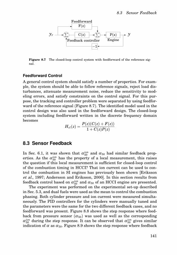
8.3 Sensor Feedback
yr∑∑
C(z) P(z)
F(z)
Feedback controller Engine
Feedforward
y
−1
Figure 8.7 The closed-loop control system with feedforward of the reference sig-nal.
Feedforward Control
A general control system should satisfy a number of properties. For exam-ple, the system should be able to follow reference signals, reject load dis-turbances, attenuate measurement noise, reduce the sensitivity to mod-eling errors, and satisfy constraints on the control signal. For this pur-pose, the tracking and controller problem were separated by using feedfor-ward of the reference signal (Figure 8.7). The identified model used in thecontrol design was also used in the feedforward design. The closed-loopsystem including feedforward written in the discrete frequency domainbecomes
Hcl(z) =P(z)(C(z) + F(z))
1 + C(z)P(z)
8.3 Sensor Feedback
In Sec. 6.1, it was shown that α ion50 and α 50 had similar feedback prop-
erties. As the α ion50 has the property of a local measurement, this raises
the question if this local measurement is sufficient for closed-loop controlof the combustion timing in HCCI? That ion current can be used to con-trol the combustion in SI engines has previously been shown [Erikssonet al., 1997; Andersson and Eriksson, 2000]. In this section results fromfeedback control based on α ion
50 and α 50 of an HCCI engine are presented.The experiment was performed on the experimental set-up described
in Sec. 5.3, and dual fuels were used as the mean to control the combustionphasing. Both cylinder pressure and ion current were measured simulta-neously. The PID controllers for the cylinders were manually tuned andthe parameters were the same for the two different feedback cases, and nofeedforward was present. Figure 8.8 shows the step response where feed-back from pressure sensor (α 50) was used as well as the correspondingα ion
50 during the step response. It can be observed that α ion50 gives similar
indication of α as α 50. Figure 8.9 shows the step response where feedback
141

Chapter 8. Control of HCCI
0 50 100 150 200 250 300 350 400
4
6
8
10
0 50 100 150 200 250 300 350 400
4
6
8
10
Control using α 50 as feedback
α50
αio
n50
Engine cycle
Figure 8.8 Step response of α when using α 50 as feedback. The thick line is thereference value of α and the figures shows α 50 (upper) and α ion
50 (lower).
0 50 100 150 200 250 300 350 400
4
6
8
10
0 50 100 150 200 250 300 350 400
4
6
8
10
Control using α ion50 as feedback
αio
n50
α50
Engine cycle
Figure 8.9 Step response of α when using α ion50 as feedback. The thick line is the
reference value of α and the figures shows α ion50 (upper) and α 50 (lower).
from the ion current sensor (α ion50 ) was used as well as the corresponding
α 50 during the step response. From Fig. 8.9, it can be noticed that the α ion50
is sufficiently robust and accurate to be used for feedback control, withsimilar performance as α 50. The step responses were both performed atan operating point of 3 bar IMEPnet, an inlet temperature of 150C, and
142
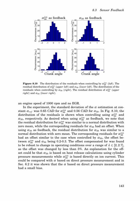
8.3 Sensor Feedback
−2 −1 0 1 20
10
20
30
40
−2 −1 0 1 20
10
20
30
40
50
−2 −1 0 1 20
10
20
30
40
−2 −1 0 1 20
10
20
30
40
50
Occ
urr
ence
s(α
ion
50)
Occ
urr
ence
s(α
50)
Occ
urr
ence
s(α
ion
50)
Occ
urr
ence
s(α
50)
Crank angleCrank angle
α ion50 as feedback α 50 as feedback
Figure 8.10 The distribution of the residuals when controlling by α ion50 (left). The
residual distribution of α ion50 (upper left) and α 50 (lower left). The distribution of the
residuals when controlling by α 50 (right). The residual distribution of α ion50 (upper
right) and α 50 (lower right).
an engine speed of 1000 rpm and no EGR.In the experiment, the standard deviation of the α estimation at con-
stant α ref was 0.65 CAD for α ion50 and 0.56 CAD for α 50. In Fig. 8.10, the
distribution of the residuals is shown when controlling using α ion50 and
α 50, respectively. As desired when using α ion50 as feedback, we note that
the residual distribution for α ion50 was similar to a normal distribution with
zero mean, while the corresponding residuals for α 50 had an offset. Whenusing α 50 as feedback, the residual distribution for α 50 was similar to anormal distribution with zero mean. The corresponding residuals for α ion
50had an offset similar to the case when controlled by α 50, the offset be-tween α ion
50 and α 50 being 0.2-0.3. The offset compensated for was foundto be robust to change in operating conditions over a range of λ ∈ [2, 2.7],as the offset was changed by less than 5%. An explanation for the off-set could be that α 50 is based on heat release calculations using cylinderpressure measurements while α ion
50 is based directly on ion current. Thiscould be compared with α based on direct pressure measurement and inSec. 6.2 it was shown that the α based on direct pressure measurementhad a small bias.
143
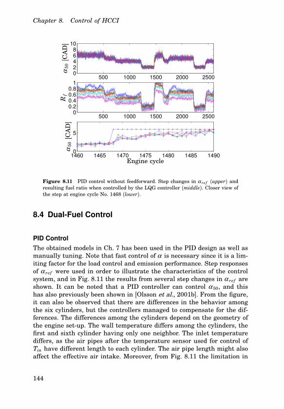
Chapter 8. Control of HCCI
500 1000 1500 2000 250002468
10
500 1000 1500 2000 25000
0.20.40.60.8
1
1460 1465 1470 1475 1480 1485 14900
5
Rf
α50
[CA
D]
Engine cycle
α50
[CA
D]
Figure 8.11 PID control without feedforward. Step changes in α ref (upper) andresulting fuel ratio when controlled by the LQG controller (middle). Closer view ofthe step at engine cycle No. 1468 (lower).
8.4 Dual-Fuel Control
PID Control
The obtained models in Ch. 7 has been used in the PID design as well asmanually tuning. Note that fast control of α is necessary since it is a lim-iting factor for the load control and emission performance. Step responsesof α ref were used in order to illustrate the characteristics of the controlsystem, and in Fig. 8.11 the results from several step changes in α ref areshown. It can be noted that a PID controller can control α 50, and thishas also previously been shown in [Olsson et al., 2001b]. From the figure,it can also be observed that there are differences in the behavior amongthe six cylinders, but the controllers managed to compensate for the dif-ferences. The differences among the cylinders depend on the geometry ofthe engine set-up. The wall temperature differs among the cylinders, thefirst and sixth cylinder having only one neighbor. The inlet temperaturediffers, as the air pipes after the temperature sensor used for control ofTin have different length to each cylinder. The air pipe length might alsoaffect the effective air intake. Moreover, from Fig. 8.11 the limitation in
144
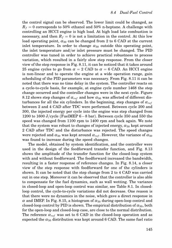
8.4 Dual-Fuel Control
the control signal can be observed. The lower limit could be changed, asR f = 0 corresponds to 50% ethanol and 50% n-heptane. A challenge withcontrolling an HCCI engine is high load. At high load late combustion isnecessary, and then R f = 0 is not a limitation in the control. At this lowload operating point, α 50 can be changed from 2 to 6 CAD at the currentinlet temperature. In order to change α 50 outside this operating point,the inlet temperature and/or inlet pressure must be changed. The PIDcontroller was tuned in order to achieve practical robustness to processvariation, which resulted in a fairly slow step response. From the closerview of the step response in Fig. 8.11, it can be noticed that it takes around25 engine cycles to go from α = 2 CAD to α = 6 CAD. An HCCI engineis non-linear and to operate the engine at a wide operation range, gainscheduling of the PID parameters was necessary. From Fig. 8.11 it can benoted that there was no time delay in the system. The controller reacts ona cycle-to-cycle basis, for example, at engine cycle number 1468 the stepchange occurred and the controller changes were in the next cycle. Figure8.12 shows step changes of α ref and how α 50 was affected of different dis-turbances for all the six cylinders. In the beginning, step changes of α ref
between 2 and 4 CAD after TDC were performed. Between cycle 200 and300, the injected energy per cycle into the engine was step changed from1200 to 1600 J/cycle (FuelMEP 6−8 bar). Between cycle 350 and 550 thespeed was changed from 1100 rpm to 1400 rpm and back again. We notethat the system was robust to changes of injected energy, α 50 kept around2 CAD after TDC and the disturbance was rejected. The speed changeswere rejected and α 50 was kept around α ref . However, the variance of α 50
was found to increase during the speed changes.The model, obtained by system identification, and the controller were
used in the design of the feedforward transfer function, and Fig. 8.13shows the amplitude of the transfer function for the closed-loop systemwith and without feedforward. The feedforward increased the bandwidth,resulting in a faster response of reference changes. In Fig. 8.14, a closerview of the step response with feedforward for one of the cylinders isshown. It can be noted that the step change from 2 to 4 CAD was carriedout in one step. Moreover it can be observed that the controller is also ableto compensate for the fuel dynamics, such as wall wetting. The variancein closed-loop and open-loop control was similar, see Table 8.1. In closed-loop control, the cycle-to-cycle variations did not decrease. One reason isthat there were no dynamics in the noise, which gave a direct response inα and IMEP. In Fig. 8.15, a histogram of α 50 during open-loop control andclosed-loop control by PID is shown. The empirical distribution of α 50, bothfor the open-loop and closed-loop case, are close to the normal distribution.The reference α ref was set to 6 CAD in the closed-loop operation and asexpected the α 50 distribution was kept around 6 CAD. The same fuel ratio
145
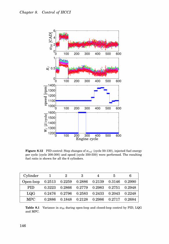
Chapter 8. Control of HCCI
0 100 200 300 400 500 6000
2
4
6
0 100 200 300 400 500 6000
0.5
1
0 100 200 300 400 500 6001000
1100
1200
1300
1400
0 100 200 300 400 500 6001200
1300
1400
1500
1600
Rf
Wf
[J/cy
cle]
α50
[CA
D]
spee
d[r
pm]
Engine cycle
Figure 8.12 PID control: Step changes of α ref (cycle 50-130), injected fuel energyper cycle (cycle 200-300) and speed (cycle 350-550) were performed. The resultingfuel ratio is shown for all the 6 cylinders.
Cylinder 1 2 3 4 5 6
Open-loop 0.2513 0.2259 0.2886 0.2139 0.3146 0.2990
PID 0.3223 0.2866 0.2779 0.2983 0.2751 0.2948
LQG 0.2476 0.2796 0.2583 0.2433 0.2043 0.2248
MPC 0.2886 0.1848 0.2128 0.2986 0.2717 0.2684
Table 8.1 Variance in α 50 during open-loop and closed-loop control by PID, LQGand MPC.
146

8.4 Dual-Fuel Control
10−2
10−1
100
101
−20
−10
0
Frequency (rad/sec)
Am
plit
ude (
dB
)
Figure 8.13 Closed-loop control without feedforward (solid). Closed-loop controlwith feedforward (dashed).
5 10 15 20
2
3
4
5
5 10 15 200.4
0.5
0.6
0.7
0.8
0.9
1
Rf
α50
[CA
D]
Engine cycle
Figure 8.14 PID control: Step change of α ref with resulting fuel ratio.
was applied to all the cylinders in the open-loop case. It can be observedthat the variance in open-loop was similar to the variance in closed-loopoperation.
LQG Control
Integral action is not inherent in LQG controller design. As integral actionwas a desired property, an error integral state was included in the process
147

Chapter 8. Control of HCCI
4 6 80
20
40
60
80
4 6 80
20
40
60
80
4 6 80
50
100
4 6 80
20
40
60
80
4 6 80
20
40
60
80
4 6 80
20
40
60
80
Occ
urr
ence
s(α
50)
Occ
urr
ence
s( α
50)
Occ
urr
ence
s(α
50)
Occ
urr
ence
s(α
50)
Occ
urr
ence
s(α
50)
Occ
urr
ence
s( α
50) Cylinder 1 Cylinder 2
Cylinder 3 Cylinder 4
Cylinder 5 Cylinder 6
Figure 8.15 Histogram of α 50 in closed-loop (dark) and in open-loop (light).
model. The estimated Kalman filter obtained from the identification wasused in the control design.
In Figure 8.16 the result from several step changes in α ref is shown.The controller was designed using the identified model in experiment 1 inSec. 7.3. The experimental conditions were the same as for the PID con-trol experiment showed in Fig. 8.11. Also the LQG controller was tuned ina robust setting. The step response performance is similar to the perfor-mance of the PID controller. As it was found in Chapter 7 that lower-ordermodels were sufficient to capture the dynamics of α 50, it is no surprisethat LQG might not give a significant improvement in comparison to PID.
Figure 8.17 shows the result of step changes of α ref and how α 50 wasaffected by different disturbances for all the six cylinders, see also Fig-ure 8.12. A feedforward was designed in order to increase the referenceresponse. Fig. 8.18 shows a closer view of the step response when feed-forward was applied for one of the cylinders. The step change from 2 to4 CAD was performed in one sample. Fig. 8.18 could be compared to Fig.8.14 as the experimental conditions were the same. The LQG controllerwas tested outside the area of the excitation data, still the controller wasable to stabilize the combustion phasing, see Fig. 8.19. As α 50 had more
148

8.4 Dual-Fuel Control
500 1000 1500 2000 250002468
10
500 1000 1500 2000 25000
0.20.40.60.8
1
1330 1335 1340 1345 1350 1355 13600
2
4
6
8
Rf
α50
[CA
D]
α50
[CA
D]
Engine cycle
Figure 8.16 LQG control without feedforward. Step changes in α ref (upper) andresulting fuel ratio when controlled by the LQG controller (middle). Closer view ofthe step at engine cycle No. 1345 (lower).
0 100 200 300 400 500 6000
2
4
6
0 100 200 300 400 500 6000
0.5
1
0 100 200 300 400 500 6001000
1100
1200
1300
1400
0 100 200 300 400 500 6001200
1300
1400
1500
1600
Rf
Wf
[J/c
ycle
]α
50[C
AD
]sp
eed
[rpm
]
Engine cycle
Figure 8.17 LQG control: Step changes of α ref (cycle 50-130), injected fuel energyper cycle (cycle 200-300) and speed (cycle 350-550) were performed. The resultingfuel ratio is shown for all the 6 cylinders.
149
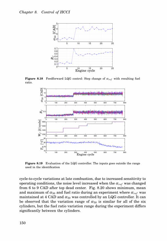
Chapter 8. Control of HCCI
5 10 15 20 25
2
3
4
5
5 10 15 20 250
0.10.20.30.40.50.60.7
Rf
α50
[CA
D]
Engine cycle
Figure 8.18 Feedforward LQG control: Step change of α ref with resulting fuelratio.
0 100 200 300 400 500 600 700 8000
5
10
15
0 100 200 300 400 500 600 700 8000
0.5
1
0 100 200 300 400 500 600 700 8001200
1400
1600
1800
0 100 200 300 400 500 600 700 80076
78
80
82
α50
[CA
D]
Rf
Wf
[J/c
ycle
]T
in[
C]
Engine cycle
Figure 8.19 Evaluation of the LQG controller. The inputs goes outside the rangeused in the identification
cycle-to-cycle variations at late combustion, due to increased sensitivity tooperating conditions, the noise level increased when the α ref was changedfrom 6 to 9 CAD after top dead center. Fig. 8.20 shows minimum, meanand maximum of α 50 and fuel ratio during an experiment where α ref wasmaintained at 4 CAD and α 50 was controlled by an LQG controller. It canbe observed that the variation range of α 50 is similar for all of the sixcylinders, but the fuel ratio variation range during the experiment differssignificantly between the cylinders.
150

8.4 Dual-Fuel Control
0 1 2 3 4 5 6 72
3
4
5
6
0 1 2 3 4 5 6 70.2
0.3
0.4
0.5
Rf
α50
[CA
D]
Cylinder
Figure 8.20 α 50 and fuel ratio for the six cylinders when the α ref was maintainedat 4 CAD. The bar for each cylinder shows the minimum, mean and maximum value.
Model Predictive Control
The identified models in Ch. 7, were used in the MPC controllers design.The tuning parameters of the MPC controllers were:
• Constraints: The control constraints were 0 ≤ R f ≤ 1 and Wf ≥ 0,and the output constraint was dp/dθ ≤ dplimit. The input con-straints were hard and the output constraint soft, and a toleranceband was specified to each constraint.
• Weights: Manipulated variable, manipulated variable rate and out-put variables. The weights also included a slack variable, ρε , usedfor relaxing the constraints.
• Horizons: The control horizons used were 1 ≤ Hu ≤ 15 and theprediction horizons used were 1 ≤ Hp ≤ 25.
• State estimation: Input noise, output noise and measurement noisewas defined and used in the calculation of the Kalman filter. Anotherapproach used, was to using the estimated Kalman filter obtainedby the identification methods used in Ch. 7.
The control of α 50 may be written as a SISO problem and Fig. 8.21 showssimulation result from step changes in the reference value of α 50 where aSISO MPC controller was used. From the figure it can be noted that thereference value was followed. At cycle 40 a disturbance in α 50 was addedand suppressed after two samples.
151
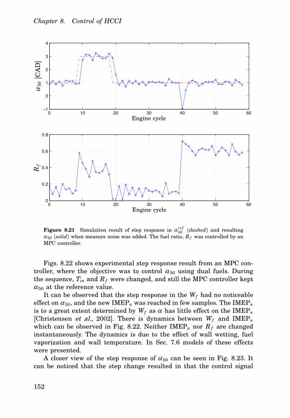
Chapter 8. Control of HCCI
0 10 20 30 40 50 60−1
0
1
2
3
4
0 10 20 30 40 50 600
0.2
0.4
0.6
0.8
α50
[CA
D]
Engine cycle
Rf
Engine cycle
Figure 8.21 Simulation result of step response in α ref50 (dashed) and resulting
α 50 (solid) when measure noise was added. The fuel ratio, R f was controlled by anMPC controller.
Figs. 8.22 shows experimental step response result from an MPC con-troller, where the objective was to control α 50 using dual fuels. Duringthe sequence, Tin and R f were changed, and still the MPC controller keptα 50 at the reference value.
It can be observed that the step response in the Wf had no noticeableeffect on α 50, and the new IMEPn was reached in few samples. The IMEPn
is to a great extent determined by Wf as α has little effect on the IMEPn
[Christensen et al., 2002]. There is dynamics between Wf and IMEPn
which can be observed in Fig. 8.22. Neither IMEPn nor R f are changedinstantaneously. The dynamics is due to the effect of wall wetting, fuelvaporization and wall temperature. In Sec. 7.6 models of these effectswere presented.
A closer view of the step response of α 50 can be seen in Fig. 8.23. Itcan be noticed that the step change resulted in that the control signal
152

8.4 Dual-Fuel Control
0 50 100 150 200 250 300 350 400 450 5000
5
10
0 50 100 150 200 250 300 350 400 450 5000
0.5
1
0 50 100 150 200 250 300 350 400 450 5002
3
4
0 50 100 150 200 250 300 350 400 450 500
1200
1400
1600
Rf
α50
[CA
D]
Engine cycle [sample]
IME
Pn
[bar
]W
f[J
]
Figure 8.22 MPC control of α 50 using fuel ratio.
60 70 80 90 100 110 120 130 140 150 160 170 1800
1
2
3
4
5
6
60 70 80 90 100 110 120 130 140 150 160 170 1800
0.2
0.4
0.6
0.8
1
Rf
α50
[CA
D]
Engine cycle [sample]
Figure 8.23 A closer view of the step response in Fig. 8.22 for cylinder 3.
was saturated at fuel ratio 1. Fuel ratio equal to one was not sufficientin order to change α 50 from 1 CAD to 4 CAD in one sample, but in thenext cycle α ref
50 was reached. At cycle 168 a negative step is applied andalso in this case the control signal was saturated. Around 4 cycles wereneeded before the desired α ref
50 was reached in this case.A fast and robust control of α is necessary in order to stabilize control
153

Chapter 8. Control of HCCI
R f α 50
Tin
n
Wf HCCI engine IMEPn
dp
dθ
Figure 8.24 The inputs and outputs of the MIMO model used in the MPC design.
an HCCI engine. It is also desired that the load, cylinder peak pressure,and emissions are controlled simultaneous. This is a MIMO control prob-lem where the controller has to be able handle constraints on several vari-ables. We will demonstrate that an MPC controller can be used to controla simplification of this MIMO problem, where the simplification consistedof not directly controlling the emissions. The HC and CO emissions werekept low by aiming at complete combustion. This was achieved by havinga early combustion phasing. The NOx emissions were no problem as thecombustion temperature was kept low in the experiments, which can beachieved by not allowing high cylinder pressure. The pressure gradientoften reaches dangerous levels for the engine and the sensors, before dan-gerous levels due to peak pressure are reached. Therefore, the magnitudeof cylinder pressure gradient was used as a safety limit instead of cylin-der peak pressure. The MIMO control problem can then be formulatedas controlling the load, without exceeding limits on the cylinder pressuregradient. The load should be reached by using the minimum amount offuel and the combustion should be complete. IMEPn is used as a measure-ment of the load.
For the MPC design, the identified MIMO model in Sec. 7.3 was used(Fig. 8.24). In order to avoid too high dp/dθ a maximum constraint wasspecified. Other constraints were the maximum and minimum constraintsof R f . Control of the load was achieved by using a weight-factor for theload. The objectives to minimize fuel consumption and having completecombustion for the desired load were achieved by weight-factors for α 50
and Wf , and by setting the reference value for α 50 to zero. This resultsin that the earliest possible combustion phasing, while still satisfying theconstraint on dp/dθ . The combustion is more complete in early combus-tion phasing than in late combustion phasing, where the cylinder volumehas increased. The increased cylinder volume will decrease the cylindertemperature, and the combustion may stop before all fuel is burned up.The manipulated variables were R f , Wf , the measured disturbances wereTin and n, and the manipulated outputs were α 50 and IMEPn. The cylinderpressure gradient was not controlled, only measured.
154

8.4 Dual-Fuel Control
0 100 200 300 400 500 600 7001.5
2
2.5
3
3.5
4
4.5
0 100 200 300 400 500 600 7005
10
15
20
25
30
IME
Pn
[bar
]d
pd
θ[b
ar/C
AD
]Engine cycles
Engine cycles
Figure 8.25 Experimental result of a step response in IMEPn, when an MIMOMPC controller was used.
As there are differences between the cylinders, cylinder individualMPC controllers were designed, and in Fig. 8.25 the result of step changesin IMEPn are shown. In this example, the constraint on dp/dθ was 20bar/CAD. It can be observed that the controller are able to control IMEPn.In Fig. 8.26, the results from one cylinder is shown. In the experiment,the reference value of IMEPn was changed from 2 bar to 4 bar in incre-ments of 0.5 bar, and the constraint on dp/dθ was 15 bar/CAD. It can beobserved that the IMEPn reference was quickly reached. A closer exami-nation of the IMEPn reference step, shown that a step response was oftenreached in 1-2 samples. It can be observed that the constraint on dp/dθwas exceeded. The constraint on dp/dθ was set to soft and the cycle-to-cycle variations were significant. Therefore, there is no guarantee that thedp/dθ constraint is not exceeded. However, dp/dθ was kept around thelimit of 15 bar/CAD, and this was mainly achieved by retarding of α 50.When R f saturate at 1, Wf was used to fulfilling the dp/dθ constraint. Asthe result the IMEPn reference of 4.5 bar was not achieved, as this wasnot possible when simultaneous satisfying the dp/dθ constraint. In orderto show some practical robustness to various disturbances, results wherethe engine speed and the θ IVC were changed are shown in Figs. 8.27 and8.28. From Fig. 8.27 it can be concluded that the MPC controller is ableto reject disturbances induced by the engine speed changes in the exper-iment. In the experiment Wf was increased from 1600 J/cycle to 1800J/cycle in order to maintain the desired IMEPn of 4 bar. This was dueto the pumping losses which increased with increasing engine speed. The
155

Chapter 8. Control of HCCI
0 100 200 300 400 500 600 700500
1000
1500
2000
0 100 200 300 400 500 600 7000
0.5
1
0 100 200 300 400 500 600 7000
2
4
0 100 200 300 400 500 600 7001
2
3
4
5
0 100 200 300 400 500 600 700
5
10
15
20
Wf
[J]
Rf
α50
[CA
D]
IME
Pn
[bar
]d
pd
θ[b
ar/C
AD
]
Engine cycles
Engine cycles
Engine cycles
Engine cycles
Engine cycles
Figure 8.26 Experimental result of a step response in IMEPn for cylinder 3, whena MIMO MPC controller was used.
156

8.4 Dual-Fuel Control
0 100 200 300 400 5001500
2000
0 100 200 300 400 5000
0.5
1
0 100 200 300 400 500
0
1
2
0 100 200 300 400 5003
4
5
0 100 200 300 400 50010
15
20
250 100 200 300 400 500
4
5
0 100 200 300 400 500
800
1000
1200
Wf
[J]
Rf
α50
[CA
D]
IME
Pn
[bar
]IM
EP
n[b
ar]
n[r
pm]
dp
dθ
[bar
]
Engine cycles
Figure 8.27 Experimental result of a speed ramp response for cylinder 3, whenan MIMO MPC controller was used.
pumping losses are significant for a turbo charged HCCI engine at highload, since a HCCI engine has low exhaust temperature [Olsson et al.,2001a].
Recall that the engine speed was included in the model. θ IVC was onthe other hand not included in the model, and the experiment shown inFig. 8.28 demonstrate practical robustness to changes in the θ IVC. The
157

Chapter 8. Control of HCCI
0 50 100 150 200 250 300 350 400 4501100
1200
1300
0 50 100 150 200 250 300 350 400 4500
0.2
0.4
0 50 100 150 200 250 300 350 400 4500
2
4
6
0 50 100 150 200 250 300 350 400 4502.5
3
3.5
0 50 100 150 200 250 300 350 400 4505
10
15
0 50 100 150 200 250 300 350 400 450
560
580
Wf
[J]
Rf
θIV
Cα
50[C
AD
]IM
EP
n[b
ar]
dp
dθ
[bar
]
Figure 8.28 Experimental result of θ IVC step responses for cylinder 3, when anMIMO MPC controller was used.
IMEPn was kept at the reference value of 3 bar.During the experiments, no problem with computational delay due to
solving the optimization problem in the MPC controller was experienced.A feature in the developed control system was that if a control signal wasnot calculated before the start of injection, a icon was lit in the GUI. Theicon was not lit more often when an MPC controller with Hu ≤ 15 wasused than for a PID controller. In practice the icon was never lit duringthe experiments in the case of Hu ≤ 15.
158
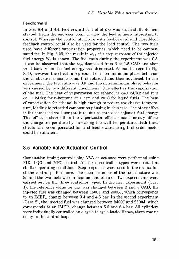
8.5 Variable Valve Actuation Control
Feedforward
In Sec. 8.4 and 8.4, feedforward control of α 50 was successfully demon-strated. From the end-user point of view the load is more interesting tocontrol. Whereas the control structure with feedforward and closed-loopfeedback control could also be used for the load control. The two fuelsused have different vaporization properties, which need to be compen-sated for. In Fig. 8.29, the result in α 50 of a step response of the injectedfuel energy Wf is shown. The fuel ratio during the experiment was 0.5.It can be observed that the α 50 decreased from 3 to 1.5 CAD and thenwent back when the fuel energy was decreased. As can be seen in Fig.8.30, however, the effect in α 50 could be a non-minimum phase behavior,the combustion phasing being first retarded and then advanced. In thisexperiment, the fuel ratio was 0.9 and the non-minimum phase behaviorwas caused by two different phenomena. One effect is the vaporizationof the fuel. The heat of vaporization for ethanol is 840 kJ/kg and it is351.1 kJ/kg for n-heptane at 1 atm and 25C for liquid fuels. The heatof vaporization for ethanol is high enough to reduce the charge tempera-ture, leading to retarded combustion phasing in this case. The other effectis the increased wall temperature, due to increased injected fuel energy.This effect is slower than the vaporization effect, since it mostly affectsthe charge temperature by increasing the wall temperature. Both theseeffects can be compensated for, and feedforward using first order modelcould be sufficient.
8.5 Variable Valve Actuation Control
Combustion timing control using VVA as actuator were performed usingPID, LQG and MPC control. All three controller types were tested atsimilar operating conditions. Step responses were used in the evaluationof the control performance. The octane number of the fuel mixture was95 and the two fuels were n-heptane and ethanol. Two experiments werecarried out on the three controller types. In the first experiment (Case1), the reference value for α 50 was changed between 2 and 5 CAD, theinjected fuel was changed between 1500J and 2000J, which correspondsto an IMEPn change between 3.4 and 4.6 bar. In the second experiment(Case 2), the injected fuel was changed between 2400J and 2600J, whichcorresponds to an IMEPn change between 5.6 and 6.4 bar. All cylinderswere individually controlled on a cycle-to-cycle basis. Hence, there was nodelay in the control loop.
159
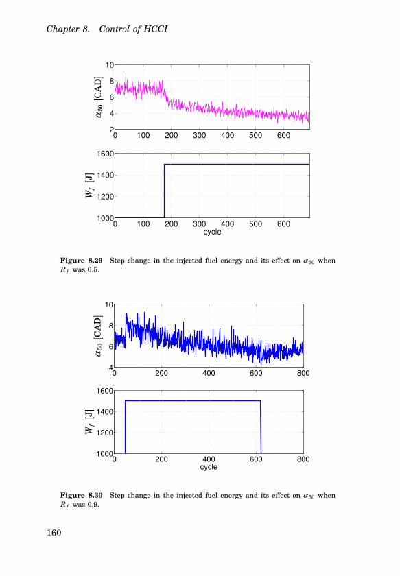
Chapter 8. Control of HCCI
0 100 200 300 400 500 6002
4
6
8
10
0 100 200 300 400 500 6001000
1200
1400
1600
cycle
α50
[CA
D]
Wf
[J]
Figure 8.29 Step change in the injected fuel energy and its effect on α 50 whenR f was 0.5.
0 200 400 600 8004
6
8
10
0 200 400 600 8001000
1200
1400
1600
cycle
α50
[CA
D]
Wf
[J]
Figure 8.30 Step change in the injected fuel energy and its effect on α 50 whenR f was 0.9.
160

8.5 Variable Valve Actuation Control
0 50 100 150 200 250 300 350 400 4500
2
4
6
8
0 50 100 150 200 250 300 350 400 450540
560
580
600
0 50 100 150 200 250 300 350 400 4501400
1600
1800
2000
α50
[CA
D]
θIV
C[C
AD
]W
f[J
]
Engine cycles
Figure 8.31 PID control of α 50 using θ IV C for Case 1.
PID
The obtained models in Ch. 7 has been used in the PID design as wellas manually tuning. The identified static nonlinearity was used for feed-forward and gain scheduling. Results from the Case 1 experiment, whenusing a PID controller is shown in Figure 8.31. The PID controller wasable to follow the reference value and compensate for the load disturbance.Note the differences between the cylinders.
In Figure 8.32, results from one of the cylinders are shown in order tobetter illustrate the step response for Case 1. Notice that the amplitudeon the control signal was decreased when the combustion phasing wasretarded. This effect was due to the nonlinearity between θ IV C and α 50.The step response was not symmetric, which is due to the dynamics ofthe cylinder wall temperature.
Results from the Case 2 experiment, when using a PID controller isshown in Figure 8.33. The PID controller was able to follow the referencevalue and compensate for the load disturbance, but the bandwidth of thecontroller was decreased. The PID controller used for Case 2 could not beused for Case 2, as it resulted in large oscillations.
In Figure 8.34, results from one of the cylinders are shown in orderto better illustrate the step response for Case 2. Note that the amplitudeon the control signal increased in comparison to the amplitude used in
161

Chapter 8. Control of HCCI
0 50 100 150 200 250 300 350 400 4501
2
3
4
5
6
7
0 50 100 150 200 250 300 350 400 450550
560
570
580
590
600
α50
[CA
D]
θIV
C[C
AD
]
Engine cycles
Figure 8.32 PID control of α 50 using θ IV C for Case 1. Result from cylinder 3.
0 50 100 150 200 250 300 350 400 450
6
8
10
12
0 50 100 150 200 250 300 350 400 450580
585
590
595
600
0 50 100 150 200 250 300 350 400 4502300
2400
2500
2600
2700
α50
[CA
D]
θIV
C[C
AD
]W
f[J
]
Engine cycles
Figure 8.33 PID control of α 50 using θ IV C for Case 2.
162

8.5 Variable Valve Actuation Control
0 50 100 150 200 250 300 350 400 4505
6
7
8
9
10
11
0 50 100 150 200 250 300 350 400 450585
590
595
α50
[CA
D]
θIV
C[C
AD
]
Engine cycles
Figure 8.34 PID control of α 50 using θ IV C for Case 2. Result from cylinder 3.
Case 1. A possible explanation is that the cycle-to-cycle variations wereincreased as the combustion phasing was retarded. The variance of α 50
became larger at later phasing.The identified static nonlinearity could also be used in the PID control
in order to linearize the system, and to make a feedforward design andgain scheduling of the controller. In Figure 8.35, step responses in α 50
are shown. From the figure it can be noted that the reference value wasfollowed and the feedforward worked well.
LQG
In the control design, the identified linear model was used. The same LQGcontroller was used for both experiment cases. Results from the Case 1experiment, when using an LQG controller is shown in Figure 8.36. TheLQG controller was able to follow the reference value and compensate forthe load disturbance. In Figure 8.37, results from one of the cylinders areshown in order to better illustrate the step response for Case 1.
The cycle-to-cycle variations is larger at later timing and this couldgive rise to oscillations. Results from the Case 2 experiment, when usingan LQG controller, where the static nonlinearity was not included in themodel and a poor linear model was used in the LQG design, is shownin Figure 8.38. In this experiment, cylinder 3 was initially stable after
163

Chapter 8. Control of HCCI
0 50 100 150 200 250 3000
5
10
0 50 100 150 200 250 300560
570
580
45 50 55 60 65 700
2
4
6
45 50 55 60 65 70565
570
575
α50
α50
θIV
Cθ
IV
C
Engine cycles
Figure 8.35 PID control of α 50 using θ IV C . The lower figures shows a closer viewof the step change.
0 50 100 150 200 250 300 350 400 4500
2
4
6
8
0 50 100 150 200 250 300 350 400 450540
560
580
600
0 50 100 150 200 250 300 350 400 4501400
1600
1800
2000
α50
[CA
D]
θIV
C[C
AD
]W
f[J
]
Engine cycles
Figure 8.36 LQG control of α 50 using θ IV C for Case 1.
164

8.5 Variable Valve Actuation Control
0 50 100 150 200 250 300 350 400 4500
1
2
3
4
5
6
7
0 50 100 150 200 250 300 350 400 450570
575
580
585
590
595
600
α50
[CA
D]
θIV
C[C
AD
]
Engine cycles
Figure 8.37 LQG control of α 50 using θ IV C for Case 1. Result from cylinder 3.
0 5 10 15 20 25 30 35 40 45 50 550
5
10
15
20
0 5 10 15 20 25 30 35 40 45 50 55550
560
570
580
590
600
α50
[CA
D]
θIV
C[C
AD
]
Engine cycles
Figure 8.38 LQG control of α 50 using θ IV C in Case 2. Result from cylinder 3.
the step change. But 20 cycles after the step change the instability wastriggered, this without any change of the controllable operation condition.Notice that the amplitude of the control signal increased very quickly andin a few cycles the process becomes unstable. The engine was automati-cally shut down, as the engine safety limit was exceeded. This exampleshows the need of accurate models.
165

Chapter 8. Control of HCCI
0 50 100 150 200 250 300 350 400 4500
2
4
6
8
0 50 100 150 200 250 300 350 400 450540
560
580
600
0 50 100 150 200 250 300 350 400 4501400
1600
1800
2000
α50
[CA
D]
θIV
C[C
AD
]W
f[J
]
Engine cycles
Figure 8.39 MPC control of α 50 using θ IV C in Case 1.
0 50 100 150 200 250 300 350 400 4500
1
2
3
4
5
6
7
0 50 100 150 200 250 300 350 400 450550
560
570
580
590
600
α50
[CA
D]
θIV
C[C
AD
]
Engine cycles
Figure 8.40 MPC control of α 50 using θ IV C in Case 1. Result from cylinder 3.
MPC
In the control design, the identified linear model was used. The sameMPC controller was use in both experiment cases. Results from the Case1 experiment, when using a MPC controller i shown in Figure 8.39. TheMPC controller was able to follow the reference value and compensate forthe load disturbance.
In Figure 8.40, results from one of the cylinders are shown in orderto better illustrate the step response for Case 1. The step response isachieved in 5-6 cycles.
Results from the Case 2 experiment, when using a MPC controller is
166
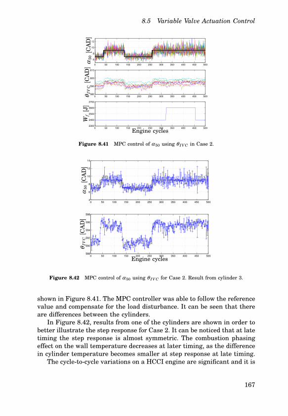
8.5 Variable Valve Actuation Control
0 50 100 150 200 250 300 350 400 450 500
6
8
10
12
0 50 100 150 200 250 300 350 400 450 500580
590
600
610
0 50 100 150 200 250 300 350 400 450 5002300
2400
2500
2600
2700
α50
[CA
D]
θIV
C[C
AD
]W
f[J
]
Engine cycles
Figure 8.41 MPC control of α 50 using θ IV C in Case 2.
0 50 100 150 200 250 300 350 400 450 5004
6
8
10
12
14
0 50 100 150 200 250 300 350 400 450 500588
590
592
594
596
598
α50
[CA
D]
θIV
C[C
AD
]
Engine cycles
Figure 8.42 MPC control of α 50 using θ IV C for Case 2. Result from cylinder 3.
shown in Figure 8.41. The MPC controller was able to follow the referencevalue and compensate for the load disturbance. It can be seen that thereare differences between the cylinders.
In Figure 8.42, results from one of the cylinders are shown in order tobetter illustrate the step response for Case 2. It can be noticed that at latetiming the step response is almost symmetric. The combustion phasingeffect on the wall temperature decreases at later timing, as the differencein cylinder temperature becomes smaller at step response at late timing.
The cycle-to-cycle variations on a HCCI engine are significant and it is
167
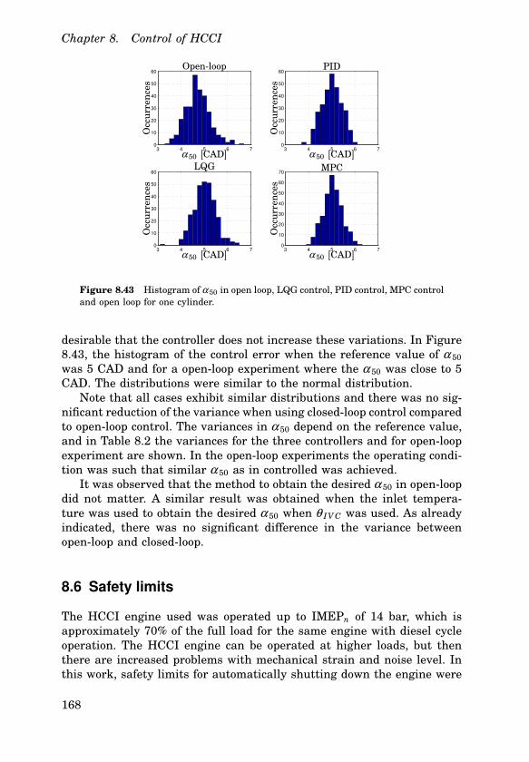
Chapter 8. Control of HCCI
3 4 5 6 70
10
20
30
40
50
60
3 4 5 6 70
10
20
30
40
50
60
3 4 5 6 70
10
20
30
40
50
60
3 4 5 6 70
10
20
30
40
50
60
70
Occ
urr
ence
s
Occ
urr
ence
s
Occ
urr
ence
s
Occ
urr
ence
s
α 50 [CAD]α 50 [CAD]
α 50 [CAD]α 50 [CAD]
Open-loop
MPCLQG
PID
Figure 8.43 Histogram of α 50 in open loop, LQG control, PID control, MPC controland open loop for one cylinder.
desirable that the controller does not increase these variations. In Figure8.43, the histogram of the control error when the reference value of α 50
was 5 CAD and for a open-loop experiment where the α 50 was close to 5CAD. The distributions were similar to the normal distribution.
Note that all cases exhibit similar distributions and there was no sig-nificant reduction of the variance when using closed-loop control comparedto open-loop control. The variances in α 50 depend on the reference value,and in Table 8.2 the variances for the three controllers and for open-loopexperiment are shown. In the open-loop experiments the operating condi-tion was such that similar α 50 as in controlled was achieved.
It was observed that the method to obtain the desired α 50 in open-loopdid not matter. A similar result was obtained when the inlet tempera-ture was used to obtain the desired α 50 when θ IV C was used. As alreadyindicated, there was no significant difference in the variance betweenopen-loop and closed-loop.
8.6 Safety limits
The HCCI engine used was operated up to IMEPn of 14 bar, which isapproximately 70% of the full load for the same engine with diesel cycleoperation. The HCCI engine can be operated at higher loads, but thenthere are increased problems with mechanical strain and noise level. Inthis work, safety limits for automatically shutting down the engine were
168

8.6 Safety limits
Table 8.2 Variances in α 50 at different reference value for the three controllers.
α 50 2 CAD 5 CAD
# Open PID LQG MPC Open PID LQG MPC
1 0.145 0.133 0.132 0.138 0.216 0.276 0.244 0.209
2 0.127 0.132 0.118 0.137 0.216 0.281 0.249 0.225
3 0.116 0.114 0.098 0.098 0.239 0.172 0.236 0.159
4 0.114 0.109 0.076 0.100 0.168 0.154 0.175 0.177
5 0.101 0.128 0.079 0.108 0.179 0.226 0.181 0.228
6 0.142 0.136 0.109 0.115 0.206 0.250 0.261 0.216
0 100 200 300 400 500 600 700 800 900 10000
50
100
150
200
0 100 200 300 400 500 600 700 800 900 100050
100
150
200
250
peak
p[b
ar]
peak
dp/d
θ[b
ar/C
AD
]
Engine cycle
Figure 8.44 Experiment where the engine safety limit was exceeded, resulting inautomatic engine shut down.
applied both on the peak pressure and on the peak pressure gradient.The medium of the last three samples was used in the safety limit check.Fig. 8.44 shows results from an experiment where the engine was auto-matically shut down. An engine needs to have a long lifespan, hence thesafety limits. The safety limits could probably be increased without imme-diate problems, but in the long run the engine and the cylinder pressuretransducer could be damaged.
169

Chapter 8. Control of HCCI
0 500 1000 1500 2000 2500
0
5
10
15
0 500 1000 1500 2000 25000
0.5
1
1.5
2
0 500 1000 1500 2000 25002
2.5
3
IME
Pn
[bar
]N
Ox
[ppm
]λ
Engine cycle
Figure 8.45 NOx emissions when the HCCI engine operates at high load IMEPn 13 bar. The engine was shut down around engine cycle 2400.
8.7 Emissions
As previously stated, the main purpose for HCCI is the promise of lowNOx emissions. Fig. 8.45 shows the resulting NOx emissions when theengine was operated at high load. It can be observed that the concentra-tions of NOx emissions are kept below 2 ppm (parts per million) and thatthe NOx emissions increased when the load increased. These values canbe considered to very low. In experiments where NOx was measured, theconcentrations of NOx never exceeded 3 ppm. These concentrations couldbe compared with the concentration of NOx in SI engines where they of-ten are few thousands ppm before aftertreatment of the emissions, andthe concentration of NOx in CI engines where the concentrations are fewhundreds of ppm before aftertreatment of the emissions. For the experi-ment shown in Fig. 8.45, the HC emissions were around 2500 ppm andthe CO emissions were around 1200 ppm. These are not low levels butmay be reduced to acceptable levels by a oxidation catalyst.
8.8 Discussion
The models used by the MPC controller were of low order, the MIMOmodel was of sixth order. There were only four constraints, three on thecontrol variables and one on the output variable dp/dθ . Therefore, the
170
8.8 Discussion
QP problem has low complexity when the control horizon is short. As theengine had fast dynamics, there was no significant improvement whenthe prediction horizon was chosen larger than ten samples, and whenthe control horizon was larger than five samples. As the computationaleffort of solving the optimization problem was small, longer horizons mayhowever be applied as it would generally increases the robustness.
At the load increased it was noticed that the NOx emissions increased,and even if the level of the NOx emissions were very low, it would beinteresting to model and control the NOx emissions. Modeling of the NOx
emissions is difficult and the measurements have long time delays.There are several commercial and research VVA systems available and
they have various degrees of freedom. The VVA system used is a researchsystem aiming for production and only the inlet port could be varied. Ifthe outlet port could also be controlled, the residual gas in the cylindercould be controlled using negative overlap. This will result in that cycle-to-cycle control of the temperature gas mixture could be controlled. Anadditional benefit is that there is no need for a heater (with the drawbackof being a more complex and expensive system). The benefit by only usingcontrol by θ IVC is that it requires a less expensive and complex system.In this comparison, a heater has low complexity and cost. The drawbackwith only using IVC is that at high load, when the combustion phasingmust be retarded in order to not damage the engine, late IVC closing maybe needed. This results in decreased volumetric efficiency, which is theopposite to what is desired when aiming towards high loads. The dualfuel approach has not this drawback. A benefit with VVA is that there isless dynamics between θ IVC and α 50 than between R f and α 50, as wallwetting and heat of vaporization does not change with θ IVC.
The PID controller is intuitive and simple controller, if comparison oftuning time needed in the design of the three different control methodswere similar.
It was found that dynamic behavior of the cylinder differs significantlyand cylinder individual-control design was necessary.
The cancellation of the nonlinearity can give rise to singularities andadd sensitivity to the noise. In practice, no such problem were experienced.
In order to have a fast and robust control of the HCCI combustionphasing in the whole operation range, it is probably necessary either toswitch or to change the controller, if linear control design methods are tobe used. Methods for this is are for example Linear Parameter Varyingsystems, Hidden Markov Models, gain scheduling or hybrid control. Otherapproaches are for instance to use nonlinear control based on nonlinearmodels, or to use adaptive control. Mean Value Engine Model can be usedin the control design for internal combustion engines [Hendricks, 1989],and in [Rausen et al., 2004] a Mean Value Model of HCCI was presented.
171
Chapter 8. Control of HCCI
8.9 Summary and Concluding Remarks
In this chapter, different control strategies, actuators and feedback alter-natives for HCCI closed-loop control were demonstrated. Previously, it wasreported that VVA can be used to control HCCI combustion. These resultswere obtained on a one-cylinder engine. The presented VVA results in thischapter, were obtained from a six-cylinder heavy duty engine. Control of asix-cylinder engine is a more difficult control problem compared to controla on-cylinder engine, as the cylinders interacts and more dynamics areadded to the system. The interactions are mainly temperature interac-tions, such as wall temperature and inlet air temperature. VVA systemscan have various degrees of freedom, and it was demonstrated that con-trol of IVC was sufficient to cycle-to-cycle control the combustion phasingin a six-cylinder heavy-duty HCCI engine.
The engine was controlled in load ranges up to 14 bar IMEPn, whichcorresponds to approximately 70% of max load, and at engine speed upto 1800 rpm. Both dual fuel and VVA can be used to cycle-to-cycle controlHCCI combustion and it was found that the HCCI engine could operate ata wider range of operation conditions by IVC, without changing the inlettemperature, than by dual fuel. Model based control, such as LQG andMPC, and PID control was successfully demonstrated to be able to controlthe HCCI dynamic, both when using VVA or dual fuel as actuator. Of thesecontrollers, MPC was found to give practically robustness in a wider rangeof operating conditions than LQG and PID controllers. When the LQG,MPC or PID controller was operated at operation condition, which wasexcited in the data from which the model used in the control design wasused, there was no significant difference in the control performance.
Cycle-to-cycle control of α 50 increased the load control performance. Inthe performed closed-loop control experiments, a step change in the loaddid not affect α 50, as the cycle-to-cycle controllers were sufficiently fast toreject the effect on α 50.
A MPC controller was proposed to solved the problem of control of theload and simultaneous minimization of the fuel consumption and emis-sions, and satisfying the constraint on dp/dθ and successful experimentwas presented.
At the operating condition of λ ∈ [2, 2.7] it was demonstrated thatfeedback based on cylinder ion current gave similar control performanceas feedback based on cylinder pressure.
172
9
Concluding Remarks
In this thesis, modeling and control of six-cylinder heavy-duty HCCI en-gine has been presented. Control of the combustion phasing is necessary inorder to generate low emissions and obtain high efficiency. The bandwidthof the controller is a limiting factor in the load and emission control. Thisthesis presents results where a reference change in combustion phasingwas achieved within a few engine cycles.
To practically use an HCCI engine it is desired that the load of theengine can be controlled and the fuel consumption should be minimized.Simultaneously, the emissions must be kept low, and the cylinder peakpressure and peak pressure gradient must be limited. One suggested so-lution to this problem is to use Model Predictive Control. Successful ex-periments demonstrating that an MPC controller could solve the problemwere performed.
Among the scientific HCCI challenges listed in Sec. 2.10, this thesishas contributed in the following areas:
Deriving dynamic models of HCCI combustion
Results that lower-order dynamic models are sufficient to describe theHCCI dynamics in the load range 2-14 bar IMEPn were presented. Itwas shown that system identification can be used as a tool for obtainingdynamic models of the combustion phasing in HCCI. It was also shownthat low-order physical models can be used to model the HCCI combustion.
Sensor and actuator studies
It was demonstrated that ion current can be used for feedback controlof the combustion phasing in an HCCI engine, for λ ∈ [2, 2.7]. An ioncurrent sensor has the benefit of being very cheap and having long life-span. Comparison of feedback alternatives of HCCI combustion phasingshowed that heat release based feedback or mass fraction burned basedfeedback were most robust in detecting the combustion phasing. Results
173

Chapter 9. Concluding Remarks
where the combustion phasing in a six-cylinder heavy-duty engine wascontrolled by either a VVA system using the inlet valve or a dual-fuelsystem was presented.
Control of combustion phasing
Control of HCCI on a cycle-to-cycle basis, where each cylinder was indi-vidually controlled, was performed on a six-cylinder heavy duty engine.The engine has been controlled in load ranges up to 14 bar IMEPn andat engine speed up to 1800 rpm. Model based control, such as LQG andMPC, and PID control was successful demonstrated.
174

10
Bibliography
Agrell, F., H.-E. Angstrom, B. Eriksson, and J. Wikander (2003): “Tran-sient control of HCCI through combined intake and exhaust valve ac-tuation.” SAE Technical Paper 2003-01-3172.
Ahmed, S., T. Tzeuch, P. Amnéus, E. Blurock, H. Soyhan, and F. Mauss(2003): PLANET D4 report, The European Community.
Amnéus, P. (2002): Homogeneous Ignition – Chemical Kinetic Studies forIC-Engine Applications. PhD thesis, Division of Combustion Physics,Lund Institute of Technology, Lund University, Lund, Sweden.
Anderson, B. D. and J. B. Moore (1990): Linear Optimal Control. PrenticeHall, Englewood Cliffs, New Jersey.
Andersson, I. and L. Eriksson (2000): “Ion sensing for combustion stabilitycontrol of a spark-ignited, direct- injected engine.” SAE TechnicalPaper 2000-01-0552.
Aoyama, T., Y. Hattori, J. Mizuta, and Y. Sato (1996): “An experimentalstudy on premixed-charge compression ignition gasoline engine.” SAETechnical Paper 960081.
Åström, K. J. and B. Wittenmark (1997): Computer Controlled Systems—
Theory and Design, Third edition. Prentice Hall, Englewood Cliffs,New Jersey.
Babajimopoulos, A., G. A. Lavoie, and D. N. Assanis (2003): “ModellingHCCI combustion with high levels of residual gas fraction - a compar-ison of two VVA strategies.” SAE Technical Paper 2003-01-3220.
Bemporad, A., F. Borelli, and M. Morari (2002): “Model predictive controlbased on linear programming-the explicit solution.” IEEE Transactionson Automatic Control, 47, pp. 1974–1985.
175

Chapter 10. Bibliography
Bengtsson, J. (2001): “Adaptive cruise control and driver modeling.”Licentiate thesis ISRN LUTFD2/TFRT--3227--SE. Department ofAutomatic Control, Lund Institute of Technology, Sweden.
Bengtsson, J., A. Ahlstrand, K. Nilsson, A. Robertsson, M. Olsson,A. Heyden, and R. Johansson (2000): “A robot playing scrabble usingvisual feedback.” In 6th Int. IFAC Symposium on Robot Control(SYROCO 2000). Vienna, Austria.
Bengtsson, J., M. Gäfvert, and P. Strandh (2004): “Modeling of hcci enginecombustion for control analysis.” In Conference in Decision and Control(CDC 2004). Bahamas.
Bengtsson, J., M. Haage, and R. Johansson (2002): “Variable time delaysin visual servoing and task execution control.” In 2nd IFAC Conferenceon Mechatronic Systems. Berkeley.
Bengtsson, J., R. Johansson, and A. Sjögren (2001): “Modeling of driverslongitudinal behavior.” In 2001 IEEE/ASME International Conferenceon Advanced Intelligent Mechatronics (AIM’01). Como,Italy.
Bengtsson, J., R. Johansson, and A. Sjögren (2002): “Modeling of driver’slongitudinal behavior.” In Johansson and Rantzer, Eds., Nonlinearand Hybrid Systems in Automotive Control, pp. 41–58. London.
Bengtsson, J. and S. Solyom (2004): “ABS and anti-skid on a LEGOcar.” Technical Report LUTFD2/TFRT --7609-- SE. Automatic Control,Lund Institute of Technology, Sweden.
Bengtsson, J., P. Strandh, R. Johansson, P. Tunestål, and B. Johansson(2004a): “Control of homogeneous charge compression ignition (HCCI)engine dynamics.” In Proceedings of the American Control Conference,pp. 4048–4053. Boston, Massachusetts.
Bengtsson, J., P. Strandh, R. Johansson, P. Tunestål, and B. Johansson(2004b): “System identification of homogenous charge compressionignition (HCCI) engine dynamics.” In IFAC Symp. Advances inAutomotive Control (AAC04), Salerno, Italy, April 19-23, 2004.
Bengtsson, J., P. Strandh, R. Johansson, P. Tunestål., and B. Johansson(2005): “Variable valve actuation for timing control of a homogeneouscharge compression ignition engine.” draft submitted to SAE WorldCongress 2005, Detroit, USA.
Bengtsson, J., P. Strandh, R. Johansson, P. Tunestål, and B. Johansson(2004): “Closed-loop combustion control of homogeneous charge com-pression ignition (HCCI) engines dynamics.” International Journal ofAdaptive Control and Signal Processing, 18, pp. 167–179.
176

Christensen, M. (2002): HCCI Combustion — Engine Operation andEmission Characteristics. PhD thesis, ISRN LUTMDN/TMHP–02/1006-SE, Department of Heat and Power Engineering, Lund Insti-tute of Technology, Lund University, Lund, Sweden.
Christensen, M., P. Einewall, and B. Johansson (1997): “Homogeneouscharge compression ignition (HCCI) using isooctane, ethanol and nat-ural gas–a comparison with spark-ignition operation.” SAE TechnicalPaper 972874.
Christensen, M., A. Hultqvis, and B. Johansson (2002): “The effect ofcombustion chamber geometry on hcci operation.” SAE Technical Paper2002-01-0425.
Christensen, M., A. Hultqvist, and B. Johansson (1999): “Demonstratingthe multi fuel capability of a homogeneous charge compression ignitionengine with variable compression ratio.” SAE Technical Paper 1999-01-3679.
Dec, J. E. and M. Sjöberg (2004): “Isolating the effects of fuel chemistryon combustion phasing in an HCCI engine and the potential of fuelstratification for ignition control.” SAE Technical Paper 2004-01-0557.
Draper, C. S. (1938): “Pressure waves accompanying detenotion in theinternal combustion engine.” J. Aeronautical Sciences, 5:6, pp. 219–226.
dSPACE (2004):. http://www.dspace.com.
Egeland, O. and J. T. Gravdahl (2002): Modeling and Simulation ForAutomatic Control. Marine Cybernetics, Trondheim, Norway.
Eriksson, L., L. Nielsen, and M. Glavenius (1997): “Closed loop ignitioncontrol by ionization current interpretation.” SAE Technical Paper970854.
European Federation for Transport and Environment (2004): Waiting forEuro 5 and Euro 6 New Emission Standards for Passenger Cars, Vansand Lorries. http://www.t-e.nu.
Fiveland, S., R. Agama, M. Christensen, B. Johansson, J. Hiltner,F. Mauss, and D. Assanis (2001): “Experimental and simulatedresults detailing the sensitivity of natural gas HCCI engines to fuelcomposition.” SAE Technical Paper 2001-01-3609.
Flierl, R., R. Hofmann, C. Landerl, T. Melcher, and H. Steyer (2001): “Derneue BMW viercylinder-Ottomotor mit valvetronic Teil 1: Konzept undkonstruktiver Aufbau.” Motortechnische Zeitschrift, No 6.
177
Chapter 10. Bibliography
Franke, A. (2002): Characterization of an Electrical Sensor for Combus-
tion Diagnostics. PhD thesis, ISRN LUTFD/TFCP–80–SE, Depart-ment of Physics, Lund Institute of Technology, Lund University, Lund,Sweden.
Gatowski, J. A., E. N. Balles, K. M. Chun, F. E. Nelson, J. A. Ekchian,and J. B. Heywood (1984): “Heat release analysis of engine pressuredata.” SAE Technical Paper 84135.
Gillbrand, P., H. Johansson, and J. Nytomt (1987): “Method and appara-tus for detecting ion current in an internal combustion engine ignitionsystem.” Technical Report. U.S. Patent No. 4,648,367.
Griffiths, J. and B. Whitaker (2002): “Thermokinetic interactions leadingto knock during homogeneous charge compression ignition.” Combus-
tion and Flame, 131:4, pp. 386–399.
Halstead, M., L. Kirsch, and C. Quinn (1977): “The autoignition ofhydrocarbon fuels at high temperatures and pressures — fitting ofa mathematical model.” Combustion and Flame, 30, pp. 45–60.
Haraldsson, G., J. Hyvonen, and P. Tunestål (2004): “HCCI closed-loopcombustion control using fast thermal management.” SAE TechnicalPaper 2004-01-0943.
Haraldsson, G., J. Hyvonen, P. Tunestål, and B. Johansson (2002):“Hcci combustion phasing in a multi-cylinder engine using variablecompression ratio.” SAE Technical Paper 2002-01-2858.
Haverkamp, B. and M. Verhaegen (1997): SMI Toolbox—State SpaceModel Identification Software for Multivariable Dynamical Systems.Dept. Electrical Engineering, Systems- and Control EngineeringGroup, TU Delft, Delft, Netherlands.
Hendricks, E. (1989): “Mean value modelling of large turbocharged two-stroke diesel engines.” SAE Technical Paper 890564.
Heywood, J. B. (1988): Internal Combustion Engine Fundamentals.McGraw-Hill, New York.
Ho, B. and R. Kalman (1966): “Effective construction of linear state-variable models from input/output pressure.” Regelungstechnik, No
14, pp. 545–548.
Hultqvist, A., M. Christensen, B. Johansson, A. Franke, M. Richter, andM. Alden (1997): “A study of the homogeneous charge compressionignition combustion process by chemoluminescence imaging.” SAETechnical Paper 1999-01-3680.
178
Hyvönen, J., G. Haraldsson, and J. Bengt (2004): “Balancing cylinder-to-cylinder variations in a multi-cylinder VCR-HCCI engine.” SAETechnical Paper 2004-01-1897.
Jeuland, N., X. Montagne, and P. Duret (2004): “New HCCI/CAI combus-tion process development: Methodolgy for determination of relevantfuel parameters.” In Which Fuels for Low CO2 Engines? IFP Interna-tional Conference.
Johansson, R. (1993): System Modeling and Identification. Prentice Hall,Englewood Cliffs, New Jersey.
Juang, J. N. and R. S. Pappa (1985): “An eigensystem realizationalgorithm for modal parameter identification and model reduction.”Journal of Guidance, Control and Dynamics, 8, pp. 620–627.
Keller PAA-21S (2004):. http://www.keller-druck.ch.
Kistler 7061 B (2004):. http://www.kistler.com.
Larimore, W. E. (1990): “Canonical variate analysis in identification,filtering and adaptive control.” In Proc. 29th IEEE Conference onDecision and Control, pp. 596–604. Honolulu.
Law, D., J. Allen, D. Kemp, G. Kirkpatrick, and T. Copland (2001):“Controlled combustion in an IC-engine with a fully variable valvetrain.” SAE Technical Paper 2001-01-0251.
Linde, L. . (2004):. http://www.leinelinde.se.
Maciejowski, J. (2002): Predictive Control with Constraints. Prentice Hall,Pearson Education, England.
Martinez-Frias, J., S. M. Aceves, D. L. Flowers, J. R. Smith, and R. W.Dibble (2000): “HCCI engine control by thermal management.” SAETechnical Paper 2000-01-2869.
Milovanovic, N., R. Dowden, R. Chen, and J. W. G. Turner (2004):“Influence of the variable valve timing strategy on the control ofa homogeneous charge compression (HCCI) engine.” SAE TechnicalPaper 2004-01-1899.
Najt, P. and D. Foster (1983): “Compression-ignited homogeneous chargecombustion.” SAE Technical Paper 830264.
Noguch, M., Y. Tanaka, T. Tanaka, and Y. Takeuchi (1979): “A study ingasoline engine combustion by observation of intermediate reactiveproducts during combustion.” SAE Technical Paper 790840.
179

Chapter 10. Bibliography
Oakley, A., H. Zhao, and N. Ladommatos (2001): “Experimental studieson controlled auto-ignition (CAI) combustion of gasoline in a 4-strokeengine.” SAE Technical Paper 2001-01-1030.
Olsson, J.-O. (2004): The HCCI Engine - High Load Performance and Con-
trol Aspects. PhD thesis, ISRN LUTMDN/TMPH–04/1019-SE, De-partment of Heat and Power Engineering, Lund Institute of Technol-ogy, Lund University, Lund, Sweden.
Olsson, J.-O., P. Tunestål, G. Haraldsson, and B. Johansson (2001a): “Aturbo charged dual fuel HCCI engine.” SAE Technical Paper 2001-01-189.
Olsson, J.-O., P. Tunestål, and B. Johansson (2001b): “Closed-loop controlof an HCCI engine.” SAE Technical Paper 2001-01-1031.
Olsson, J.-O., P. Tunestål, B. Johansson, S. Fiveland, J. R. Agama, andD. N. Assanis (2002a): “Compression ratio influence on maximum loadof a natural gas HCCI engine.” SAE Technical Paper 2002-01-0111.
Olsson, T., J. Bengtsson, R. Johansson, and H. Malm (2002b): “Forcecontrol and visual servoing using planar surface identification.” InIEEE Int. Conference on Robotics and Automation, pp. 4211–4216.Washington D.C., USA.
Olsson, T., J. Bengtsson, A. Robertsson, and R. Johansson (2003):“Visual position tracking using dual quaternions with hand-eye motionconstraints.” In IEEE Int. Conference on Robotics and Automation,pp. 3491–3496. Taipei, Taiwan.
Onishi, S., S. H. Jo, K. Shoda, P. D. Jo, and S. Kato (1979): “Activethermo—atmosphere combustion (ATAC)–a new combustion processfor internal combustion engines.” SAE Technical Paper 790501.
Pentronic (2004):. www.pentronic.com/.
Pischinger, M., W. Salber, F. V. D. Staay, H. Baumgarten, and H. Kemper(2000): “Benefits of the electromechanical valve train in vehicleoperation.” SAE Technical Paper 2000-01-1223.
Rassweiler, G. and L. Withrow (1938): “Motion pictures of engine flamescorrelated with pressure cars.” SAE Transactions, 42:5, pp. 185–204.
Rausen, D. J., A. G. Stefanopoulou, J.-M. Kang, J. A. Eng, and T.-W.Kuo (2004): “A mean-value model for control of homogeneous chargecompression ignition (HCCI) engines.” In Proceedings of the AmericanControl Conference, pp. 125–131.
180

Reinmann, R. (1998): Theoretical and Experimental Studies of theFormation of Ionized Gases in Spark Ignition Engines. PhD thesis,ISRN LUTFD2/TFCP –37–SE, Department of Physics, Lund Instituteof Technology, Lund University, Lund, Sweden.
Richter, M., A. Franke, J. Engström, A. Hultqvist, B. Johansson, andM. Alden (2000): “The influence of charge inhomogeneity on the HCCIcombustion process.” SAE Technical Papers 2000-01-2868.
Roth, K., A. Sobiesiak, L. Robertson, and S. Yates (2002): “In-cylinderpressure measurements with optical fiber and piezoelectric pressuretransducers.” SAE Technical Paper 2002-01-0745.
Ryan, T. and T. Callahan (1996): “Homogeneous charge compressionignition of diesel fuel.” SAE Technical Paper 961160.
Sellnau, M., F. Matekunas, P. Battiston, C.-F. Chang, and D. Lancaster(2000): “Cylinder-pressure-based engine control using pressure- ratio-management and low-cost non-intrusive cylinder pressure sensors.”SAE Technical Paper 2000-01-0932.
Shaver, G. M., J. C. Gerdes, P. Jain, P. Caton, and C. Edwards (2003):“Modeling for control of HCCI engines.” In Proceedings of the AmericanControl Conference, pp. 749–754. Denver, Colorado.
Shaver, G. M., J. C. Gerdes, and M. Roelle (2004): “Physics-based closed-loop control of phasing, peak pressure and work output in HCCIeninges utilizing variable valve actuation.” In Proceedings of theAmerican Control Conference, pp. 150–155. Boston, Massachusetts.
Shimasaki, Y., M. Kobayashi, H. Sakamoto, M. Ueno, M. Hasegawa,H. Yamaguchi, and T. Suzuki (2004): “Study on engine managementsystem using in-cylinder pressure sensor integrated with spark plug.”SAE Technical Paper 2004-01-0519.
Sjöberg, M. and J. Dec (2003): “Combined effects of fuel-type and enginespeed on intake temperature requirements and completeness of bulg-gas reactions for HCCI combustion.” SAE Technical Paper 2003-01-3173.
Strandh, P., J. Bengtsson, M. Christensen, R. Johansson, A. Vressner,P. Tunestål, and B. Johansson (2003): “Ion current sensing for HCCIcombustion feedback.” SAE Technical Paper 2003-01-3216.
Strandh, P., J. Bengtsson, R. Johansson, P. Tunestål., and B. Johansson(2004): “Cycle-to-cycle control of a dual-fuel HCCI engine.” SAETechnical Paper 2004-01-0941.
181

Chapter 10. Bibliography
Tanaka, S., F. Ayala, and J. Keck (2003a): “A reduced chemical kineticmodel for HCCI combustion of primary reference fuels in a rapidcompression machine.” Combustion and Flame, 133, pp. 467–481.
Tanaka, S., F. Ayala, J. Keck, and J. Heywood (2003b): “Two-stageignition in HCCI combustion and HCCI control by fuels and additives.”Combustion and Flame, 132, pp. 219–239.
Theobald, M., B. Lequesne, and R. Henry (1994): “Control of engine loadvia electromagnetic valve actuators.” SAE Technical Paper 940816.
Thurns, S. R. (1996): An introduction to combustion. McGraw-Hill,Singapore.
Tunestål, P. (2001): Estimation of the In-Cylinder Air/Fuel Ratio of anInternal Combustion Engine by the Use of Pressure Sensors. PhDthesis, ISRN LUTMDN/TMVK–1025-SE, Department of Heat andPower Engineering, Lund Institute of Technology, Lund University,Lund, Sweden.
U.S. Environmental Protection Agency (2000): 2007 emission standardfor Heavy-Duty Truck and Bus Engines. http://www.epa.gov.
Verhaegen, M. (1994): “Identification of the deterministic part of MIMOstate space models.” Automatica, 30, pp. 61–74.
Vibe, I. I. (1970): Brennverlauf und Kreisprozessrechnung. VEB VerlagTechnik Berlin.
Vressner, A., A. Lundin, P. Tunestål, and J. B. (2003): “Pressure oscilla-tions during rapid HCCI combustion.” SAE Technical Paper 2003-01-3217.
Vressner, A., P. Strandh, A. Hultqvist, P. Tunestål, and B. Johansson(2004): “Multiple point ion current diagnostics in an HCCI engine.”SAE Technical Paper 2004-01-0934.
Woschni, G. (1967): “A universally applicable equation for instantaneousheat transfer coefficient in the internal combustion engine.” SAETechnical Paper 670931.
xPC Target (2004):. http://www.mathworks.com/products/xpctarget/.
Yelvington, P. and W. Green (2003): “Prediction of the knock limitand viable operating range for a homogeneous-charge, compression-ignition (HCCI) engine.” SAE Technical Paper 2003-01-1092.
182

A
Appendix
A.1 Air-fuel ratio, λ
The Air-fuel ratio value is relative to the actual measured condition andthe stoichiometric condition.
λ =
(mair
m f uel
)actual(
mair
m f uel
)stoich
where mair is the mass flow to the engine and m f uel is the injected fuelto the engine.
A.2 Mean Effective Pressure
The indicated work per cycle is obtained by integrating around the curvein a p-V diagram. There are two different definitions of indicated output:
Gross indicated work per cycle, IM EPn. Work delivered to the pistonover the compression and expansion strokes only.
IM EPn =1
VD
∮ expan
comp
pdV (A.1)
where VD is the displacement volume.Net indicated work per cycle, IM EPn. Work delivered to the piston
over the entire four-stroke cycle, intake, compression, expansion and blow-down stroke.
IM EPnet =1
VD
∮ Blow
Intake
pdV (A.2)
183

Appendix A. Appendix
The Fuel Mean Effective Pressure, FuelMEP, is defined as
FuelMEP =m f QLVH
Vd
(A.3)
where m f is the mass of fuel supplied per cycle, QLVH is the lower heatingvalue for the fuel, and Vd is the displacement volume of the engine.
184