Climate Change Impact Phase II - NYISO
98
Climate Change Impact Phase II An Assessment of Climate Change Impacts on Power System Reliability in New York State FINAL REPORT Authors: Paul J. Hibbard Charles Wu Hannah Krovetz Tyler Farrell Jessica Landry September 2020 Draft September 2, 2020
Transcript of Climate Change Impact Phase II - NYISO

Climate Change Impact Phase II
An Assessment of Climate Change Impacts on Power System Reliability in New York State FINAL REPORT
Authors:
Paul J. Hibbard
Charles Wu
Hannah Krovetz
Tyler Farrell
Jessica Landry
September 2020
Draft August 18, 2020
Climate Change Impact Phase II
An Assessment of Climate Change Impacts on Power System Reliability in New York State FINAL REPORT
Authors:
Paul J. Hibbard
Charles Wu
Hannah Krovetz
Tyler Farrell
Jessica Landry
September 2020
Draft August 18, 2020
Climate Change Impact Phase II
An Assessment of Climate Change Impacts on Power System Reliability in New York State FINAL REPORT
Authors:
Paul J. Hibbard
Charles Wu
Hannah Krovetz
Tyler Farrell
Jessica Landry
September 2020
Draft September 2, 2020

Climate Change Phase II September 2020
Analysis Group, Inc.
Acknowledgments
This report has been prepared at the request of the New York Independent System Operator (NYISO), and presents an
assessment of the potential impacts on power system reliability in 2040 associated with system changes due to climate change
and policies to mitigate its effects. Our work benefitted significantly from input and comment from the NYISO and its market
participants and stakeholders.
About the Authors
Paul Hibbard is a former Chairman of the Massachusetts Public Utilities Commission, and has held positions in both energy and
environmental agencies in Massachusetts. During his tenure on the Commission, Mr. Hibbard served as a member of the
Massachusetts Energy Facilities Siting Board, and has testified before Congress, state legislatures, and federal and state
regulatory agencies. Mr. Hibbard is now a Principal in Analysis Group’s Boston office, and has public and private sector
experience in energy and environmental technologies, economics, market structures, and policy.
Charles Wu, a Manager in Analysis Group’s Boston office, is an expert in the assessment and design of wholesale electricity
markets in Northeastern U.S. power market regions. Mr. Wu’s work has included review and analysis of generating unit
performance in and design parameters affecting capacity and energy markets in New England and New York; the development
of power market models to evaluate unit performance and profitability; and the assessment of changing infrastructure and
public policy on economic, consumer and environmental impacts through economic and production cost modeling.
Hannah Krovetz is a Senior Analyst in Analysis Group’s San Francisco office, with experience in the application of economic
analyses to challenges in energy and environmental markets and policy. Ms. Krovetz has focused in recent years on technical
analysis and systems modeling related to power sector market design, power system reliability, and energy/climate policy
matters.
Tyler Farrell is an Analyst in Analysis Group’s Boston office, with background in evaluating the economic and financial aspects of
electricity generation from both individual business and system operator perspectives. Mr. Farrell has focused in recent years
on the design and implementation of models to evaluate wholesale market and reliability outcomes in the electric sector.
Jessica Landry is an Analyst in Analysis Group’s Boston office, with background in the application of econometrics to the
evaluation of international monetary issues, higher education, and antitrust/competition matters. Ms. Landry has recently
focused on the emergence of the offshore wind sector in the Eastern U.S., and the refinement of power system modeling data
and logic.
About Analysis Group
Analysis Group is one of the largest international economic consulting firms, with more than 1,000 professionals across 14
offices in North America, Europe, and Asia. Since 1981, Analysis Group has provided expertise in economics, finance, health
care analytics, and strategy to top law firms, Fortune Global 500 companies, government agencies, and other clients worldwide.
Analysis Group’s energy and environment practice area is distinguished by expertise in economics, finance, market modeling
and analysis, regulatory issues, and public policy, as well as deep experience in environmental economics and energy
infrastructure development. Analysis Group has worked for a wide variety of clients including (among others) energy
producers, suppliers and consumers, utilities, regulatory commissions and other federal and state agencies, tribal governments,
power‐system operators, foundations, financial institutions, and start‐up companies.

Climate Change Phase II September 2020
Analysis Group, Inc. Page 1
Table of Contents
I. Executive Summary 6 Background and Approach ........................................................................................................................... 6 Results and Observations ............................................................................................................................. 8
II. Analytic Method 16 Overview of Analytic Method .................................................................................................................... 16 Framework for Energy Balance Analysis .................................................................................................... 18 Construction of Seasonal Modeling Periods and Load Scenarios .............................................................. 19 1. Load Scenarios ........................................................................................................................................... 19 2. Seasonal Modeling Periods ........................................................................................................................ 20 Construction of Resource Sets by Load Case ............................................................................................. 21 1. Retention of Baseload Resources .............................................................................................................. 22 2. Renewable Resources (CARIS Starting Point) ............................................................................................ 23 3. Renewable Resource: Additions to 2040 ................................................................................................... 24 4. Imports from Neighboring Areas ............................................................................................................... 25 5. Modulation of EV Load Shape.................................................................................................................... 26 6. Increase in Inter‐zonal Transfer Capability ................................................................................................ 28 7. Energy Storage Resources ......................................................................................................................... 29 8. Price Responsive Demand ......................................................................................................................... 32 9. Dispatchable and Emissions‐Free Resource .............................................................................................. 32 10. Resource Set Summaries ........................................................................................................................... 34
Representation of Electric System Operations .......................................................................................... 36 1. Transfer and Dispatch Logic ....................................................................................................................... 36 2. Use of Dispatchable and Emissions‐Free Resources .................................................................................. 36
Comparisons with Grid in Transition Resource Sets .................................................................................. 36
IV. Cases Analyzed: Combinations of Load Scenarios and Physical Disruptions 38 Physical Disruptions: Interruptions of Resources and Transmission ......................................................... 38 1. Temperature Waves .................................................................................................................................. 38 2. Wind Lulls .................................................................................................................................................. 42 3. Storm Scenarios ......................................................................................................................................... 45 4. Other Climate Impacts ............................................................................................................................... 49
Construction of Combination Cases ........................................................................................................... 49
V. Output Metrics 51 Model Output ............................................................................................................................................. 51 Analysis of Outcomes ................................................................................................................................. 56
VI. Results and Observations 57 Overview .................................................................................................................................................... 57 Baseline Scenario Results ........................................................................................................................... 57 1. A Note About Starting Point Resource Sets ............................................................................................... 57 2. Aggregate Load/Generation Balance ......................................................................................................... 59 3. Peak Hour Patterns .................................................................................................................................... 63 4. Ramping Patterns ...................................................................................................................................... 64 5. Aggregate Use of Dispatchable and Emissions‐free Resources ................................................................. 66
Key Observations by Physical Disruption ................................................................................................... 67 1. Temperature Waves .................................................................................................................................. 68 2. Wind Lulls .................................................................................................................................................. 69

Climate Change Phase II September 2020
Analysis Group, Inc. Page 2
3. Storm Scenarios ......................................................................................................................................... 71 4. Other Climate Impacts ............................................................................................................................... 71 5. Case Result Summaries: ............................................................................................................................. 72 Cross‐Seasonal Effects ................................................................................................................................ 73 Comparisons of Results with Grid in Transition Resource Set ................................................................... 75 Pace of Resource Change ........................................................................................................................... 79 Observations .............................................................................................................................................. 82
VII. References 86
VIII. Glossary 88
IX. Technical Appendices 89 Input Data to Electric System Model.......................................................................................................... 89 1. Phase I Load Data ....................................................................................................................................... 89 2. NREL wind and solar profiles ..................................................................................................................... 91 3. NREL data for wind lulls ............................................................................................................................. 94
Loss of Load Duration Curves for all Scenarios and Physical Disruptions ................................................ 114 Diagnostic Charts for All Cases ................................................................................................................. 113

Climate Change Phase II September 2020
Analysis Group, Inc. Page 3
Figures
Figure ES‐1: Energy Balance Model (EBM) Inputs and Outputs .................................................................................... 7
Figure ES‐2: Hourly Load/Generation Balance, CCP2‐CLCPA Winter Wind Lull Case .................................................. 11
Figure ES‐3: Maximum Hourly Ramping Requirement, CCP2‐CLCPA Winter Case ...................................................... 12
Figure 4: Structure of Analysis ..................................................................................................................................... 16
Figure 5: Energy Balance Model Steps and Data Sources ............................................................................................ 17
Figure 6: Imports During Modeling Period .................................................................................................................. 26
Figure 7: Electric Vehicle Daily Load Shape from Phase I Study .................................................................................. 27
Figure 8: Electric Vehicle Daily Load Shape Adjusted for Off‐peak Charging .............................................................. 27
Figure 9: Simplified Transmission Map and Limits (Starting Point) ............................................................................. 29
Figure 10: Battery and Renewables Location (CCP2 ‐ CLCPA) ..................................................................................... 31
Figure 11: Battery and Renewables Location (CCP2 ‐ Reference) ............................................................................... 31
Figure 12: Simplified Transmission Map and Limits, CCP2‐CLCPA ............................................................................... 34
Figure 13: Simplified Transmission Map and Limits, CCP2‐Reference ........................................................................ 35
Figure 14: Example of Heat Wave Increased Load: CLCPA Summer Load Scenario .................................................... 39
Figure 15: Example of Heat Wave Decreased Wind Production: CLCPA Summer Load Scenario ............................... 40
Figure 16: Heat Wave Solar Production: CLCPA Summer Load Scenario .................................................................... 41
Figure 17: Wind Farm Locations used in Wind Lull Analysis ........................................................................................ 42
Figure 18: Summer Wind Lull Example ‐ Summer 2007 Average Daily Wind Shape .................................................. 44
Figure 19: Example of Wind Lull Decreased Wind Production: CLCPA Summer Load Scenario .................................. 45
Figure 20: NYISO‐Metered Load during Hurricane Sandy and Recovery Period ......................................................... 46
Figure 21: Cumulative Generating Capacity Recovery during Hurricane Sandy Recovery Period ............................... 47
Figure 22: Cumulative Transmission Recovery during Hurricane Sandy Recovery Period .......................................... 47
Figure 23: Example of Hourly Results Summary .......................................................................................................... 52
Figure 24: Example of Full Period Results Summary ................................................................................................... 53
Figure 25: Example of NYCA Hourly Generation by Fuel Group .................................................................................. 54
Figure 26: Example of Generation by Resource Type Over Modeling Period ............................................................. 54
Figure 27: Example of NYCA DE Resources Generation Duration ............................................................................... 55
Figure 28: Example of NYCA Loss of Load Occurrences Duration ................................................................................ 55
Figure 29: Battery and Pumped Storage Energy Level, CCP2‐CLCPA Winter ............................................................... 60
Figure 30: Hourly Load/Generation Balance, CCP2‐CLCPA Winter .............................................................................. 60
Figure 31: Generation by Resource Type, CCP2‐CLCPA Winter ................................................................................... 61
Figure 32: Hourly Load/Generation Balance, CCP2‐CLCPA Summer ........................................................................... 61
Figure 33: Generation by Resource Type, CCP2‐CLCPA Summer ................................................................................ 62
Figure 34: Hourly Load/Generation Balance, CCP2‐CLCPA Shoulder .......................................................................... 62
Figure 35: Generation by Resource Type, CCP2‐CLCPA Shoulder ................................................................................ 63
Figure 36: Resource Mix during Seasonal Peak Load Hours (CCP2‐CLCPA Case)......................................................... 64
Figure 37: Average Load and Generation Requirements, CCP2‐CLCPA Winter ........................................................... 65
Figure 38: Maximum Hourly Ramping Requirement, CCP2‐CLCPA Winter ................................................................. 66
Figure 39: Duration Curve of DE Resource Generation by Modeling Period ............................................................... 67
Figure 40: Hourly Load/Generation Balance, CCP2‐CLCPA Summer Heat Wave Case ................................................ 68
Figure 41: Hourly Load/Generation Balance, CCP2‐CLCPA Winter Cold Wave Case ................................................... 69
Figure 42: Hourly Load/Generation Balance, CCP2‐CLCPA Winter Wind Lull Case ..................................................... 70
Figure 43: Hourly Load/Generation Balance, CCP2‐CLCPA Summer Wind Lull Case ................................................... 70
Figure 44: Hourly Load/Generation Balance, CCP2‐CLCPA Summer Hurricane Case .................................................. 71

Climate Change Phase II September 2020
Analysis Group, Inc. Page 4
Figure 45: Resource Mix during Seasonal Peak Load Hours (CLCPA Case), CCP2‐CLCPA Resource Set ....................... 74
Figure 46: Winter Generation by Resource Type – CCP2‐CLCPA ................................................................................. 76
Figure 47: Winter Generation by Resource Type – GIT‐CLCPA .................................................................................... 76
Figure 48: Summer Generation by Resource Type ‐ CLCPA Case with CCP2 Resource Set ......................................... 78
Figure 49: Summer Generation by Resource Type ‐ CLCPA Case with Grid in Transition Resource Set ...................... 78
Figure 50: Historical Resource Mix in New York, 2011‐2020 ....................................................................................... 80
Climate Change Phase II September 2020
Analysis Group, Inc. Page 5
Tables
Table ES‐1: Generation Capacity, CLCPA Resource Set.................................................................................................. 9
Table ES‐2: Case Result Summaries ............................................................................................................................. 10
Table ES‐3: Excess Renewable Generation .................................................................................................................. 13
Table ES‐4: Required Rate of New Resource Development ........................................................................................ 14
Table 5: Summary of Load by Seasonal Modeling Period ............................................................................................ 20
Table 6: Renewable Capacity Factor by Season ......................................................................................................... 24
Table 7: Renewable Capacity by Resource Set .......................................................................................................... 25
Table 8: Transmission Limits by Resource Set ............................................................................................................. 28
Table 9: Generation Capacity, CCP2‐CLCPA ................................................................................................................. 34
Table 10: Generation Capacity, CCP2‐Reference ......................................................................................................... 35
Table 11: Resource Sets from Grid in Transition Study ............................................................................................... 37
Table 12: Description of Physical Disruption Modeling .............................................................................................. 38
Table 13: Historical Summer Wind Lulls from NREL data, 2007‐2012, ≤15 percent Implied Capacity Factor ............ 43
Table 14: Historical Winter Wind Lulls from NREL data, 2007‐2012, ≤25 percent Implied Capacity Factor .............. 43
Table 15: List of Modeled Combination Cases............................................................................................................. 50
Table 16: DE Resource Capacity Factor by Season ...................................................................................................... 67
Table 17: Curtailed “Excess” Renewable Generation by Seasonal Modeling Period, CLCPA Load Scenario, CCP2‐
CLCPA Resource Set ..................................................................................................................................................... 73
Table 18: Curtailed “Excess” Shoulder Month Renewable Generation by Load Scenario and Resource Set .............. 73
Table 19: Shoulder Month Energy Potential as Compared to DE Resource Use, CCP2 Resource Set ......................... 75
Table 20: Transmission Constrained Hours, CCP2‐CLCPA Winter Baseline Case ......................................................... 77
Table 21: Comparison of Case Results by Resource Set , Winter CLCPA ..................................................................... 77
Table 22: Transmission Constrained Hours ‐ Summer CLCPA Baseline Case ............................................................... 79
Table 23: Comparison of Case Results by Resource Set ‐ Summer CLCPA .................................................................. 79
Table 24: Required Pace of Development to Meet 2040 Resource Set Quantities ..................................................... 81

Climate Change Phase II September 2020
Analysis Group, Inc. Page 6
I.Executive Summary
Background and Approach
In 2020, NYISO contracted with Analysis Group (AG) to complete this Climate Change Phase II Study (“Phase II
Study”). The Phase II Study is designed to review the potential impacts on power system reliability of the (1) the
electricity demand projections for 2040 developed in the preceding Climate Change Phase I Study,1 and (2) potential impacts on system load and resource availability associated with the impact of climate change on the
power system in New York (“climate disruptions”).The climate disruptions considered include items that could
potentially occur or intensify with a changing climate and that affect power system reliability, such as more
frequent and severe storms, extended extreme temperature events (e.g., heat waves and cold snaps), and other
meteorological events (e.g., wind lulls, droughts, and ice storms).
Notably, the 2019 New York State Climate Leadership and Community Protection Act (CLCPA) requires “…reducing
100% of the electricity sector’s greenhouse gas emissions by 2040.”2 This means that step one in our analysis was
the development of a “starting point” Climate Change Phase II resource set (the “CCP2 resource set”) for the year
2040, one that starts with the Congestion Assessment and Resource Integration Study (CARIS) 70x30 resources,
but by 2040 meets the requirements of the CLCPA. Given the extensive reliance today on generators that burn
fossil fuels (primarily natural gas), a key input to the analysis was the establishment of a resource set that does not
include the operation of existing fossil‐fueled thermal power plants, yet has sufficient resources available to meet
electricity demand in the year 2040 without emissions of greenhouse gases (GHG).
With these key parameters in mind, over the past nine months Analysis Group has carried out its analysis of
climate change‐related impacts to system reliability. This report summarizes the results of our analysis, and
presents the purpose, analytic method, and observations drawn from AG’s review. The project was completed
with assistance from NYISO with respect to system data and analyses, and with input from stakeholders at the
NYISO Electric System Planning Working Group (ESPWG) and the Transmission Planning Advisory Subcommittee
(TPAS).
Ultimately, the purpose of this Phase 2 study is to simulate the potential impacts of climate change and climate
policy on the reliable operation of the New York power system, and to present observations to enable the NYISO,
market participants, policy makers and other stakeholders an opportunity to consider whether the potential
impacts warrant changes to planning, operational practices, and/or market designs. Analysis Group’s approach to
the analysis is presented in detail in Section II. In summary, it consists of the following steps (depicted in Figure ES‐
1):
1 In 2019, the New York Independent System Operator (NYISO) contracted with Itron to complete long‐term energy, peak, and hourly load projections for
the New York Control Area through the year 2050. The projections capture the impact of climate change on average temperatures and electricity
demand, as well as the potential impact on demand of increased energy efficiency and electrification of the building and transportation sectors. That
project ‐ termed the Climate Change Phase I Study (“Phase I Study”) ‐ was completed in 2019, and included long‐term energy, peak, and hourly load
projections (for the NYISO system as a whole and each of the eleven NYISO load zones) that reflect the potential demand impacts of climate change and
climate policy in New York. Itron, New York ISO Climate Change Impact Study; Phase 1: Long‐Term Load Impact, December 2019. 2 New York Climate Leadership and Community Protection Act (CLCPA), NY State Senate Bill S6599, 2019‐06‐18. The New York Department of
Environmental Conservation (DEC) proposes to define GHGs as the following: GHGs are “[g]aseous constituents of the atmosphere that absorb and emit
radiation at specific wavelengths within the spectrum of terrestrial radiation emitted by the Earth's surface, the atmosphere itself, and by clouds. For the
purposes of the Part, this includes carbon dioxide, methane, nitrous oxide, perfluorocarbons, hydrofluorocarbons, and sulfur hexafluoride.”
https://www.dec.ny.gov/regulations/121059.html.

Climate Change Phase II September 2020
Analysis Group, Inc. Page 7
‐ Configure Analysis Group’s Energy Balance Model
(EBM) to simulate power system operations in
2040, with separate balancing across and within
11 NYISO load zones;
‐ Review and input the ITRON Phase I hourly load
forecasts for 2040, and extract data from the
Phase I analysis to enable the modeling of changes
in electricity demand with changes in
meteorological conditions (e.g., temperature);
From each Phase I forecast we evaluate the peak‐
demand month in the winter (January) and
summer (July), and the low‐demand month in the
shoulder season (April);
‐ Review state requirements encoded in the CLCPA,
and consider potential scenarios for resource
development consistent with state requirements
and current technology trends;
‐ Based on this review, identify principles for
constructing resource sets with sufficient
resources to reliably meet NYISO seasonal peak
demand, building on the 2019 CARIS Phase I 70X30
Case;
‐ Develop four cases to analyze, incorporating two
Phase I Itron 2040 load forecasts (the “Reference
Case” and the “CLCPA Case”) and 2040 resource sets that reliably meet demand for each forecast: two
that were developed for this Phase II Study, and two that were developed as part of the Grid in Transition
(GIT) study.3 Thus, the four cases analyzed are:
o CCP2‐Reference
o CCP2‐CLCPA
o GIT‐Reference
o GIT‐CLCPA
‐ Include in the resource sets a generic resource, the role of which is to identify the attributes of any
additional resources that may be needed to avoid or reduce Loss of Load Occurrences (LOLO).4 These
resources ‐ identified as dispatchable and emissions‐free resources (“DE Resources”) ‐ are described in
more detail below;
3 The review of resource sets from both studies is intended to highlight differences in potential resource development pathways. The CCP2 resource sets
are focused on achieving the CLCPA 2040 requirements with a primary focus on expansion of renewable resources and associated transmission. The GIT
resource sets reflect less infrastructure development, and a stronger focus on resources like existing thermal generating resources operating on zero
carbon fuels. See Section II for a more detailed description of the resource sets. 4 Loss of Load Occurrences are not meant to be equivalent to Loss of Load Equivalent in a resource adequacy context.
Figure ES‐1: Energy Balance Model (EBM) Inputs and Outputs

Climate Change Phase II September 2020
Analysis Group, Inc. Page 8
‐ Identify the potential impacts of a changing climate on the power system, including conditions or events
that alter electricity demand, generating resource availability and operations, and inter‐zonal
transmission transfer capability. This research is used to construct “climate disruption scenarios”;
‐ Run the climate disruption scenarios through Analysis Group’s EBM for each of the four cases analyzed
(the CCP2‐Reference, CCP2‐CLCPA, GIT‐Reference, and GIT‐CLCPA), for each seasonal month (where
relevant);5 and
‐ Generate results with respect to potential loss of load occurrences (LOLO) and reliance on DE resources,
and draw observations related to power system operations based on the comparison of results across
cases.
Section II contains a detailed summary of our analytic method, and of the structure and mechanics of the Analysis
Group Energy Balance Model. Section III describes the cases we analyze, which include the climate change‐
induced physical disruptions layered on the four different cases. In Section IV we provide an overview of the
metrics we evaluate through the EBM, and the form of model outputs for each case. Finally, in Section V we
present the results of the analysis and our observations based on the results. The Appendices contain additional
modeling details and a comprehensive set of results across all relevant cases and climate disruption scenarios.
Results and Observations
The context for our analysis includes both the impact of a changing climate on power system operations, and the
energy and environmental policy response to the threat of climate change. In recent years, many states have
moved towards establishing significant and progressive GHG emission reduction requirements that are
directionally consistent with dramatically reducing GHGs from energy supply and use by the middle of the century,
across all sectors of the economy. With the passage of the CLCPA, New York positioned itself at the forefront of
these efforts to address climate change and initiated a fundamental transition in energy supply and use in general,
and in the electric system in particular.
It is difficult to envision the specific pathway New York will take to achieve the required GHG emission reductions
from the economy over just the next three decades, and from the electric sector over the next two decades. The
scope of changes that will be needed to the state’s building, transportation and electric sectors is unprecedented.
Meeting this level of emission reductions will not only require rapid advancement of existing advanced energy
technologies, but will also likely require technologies, policies, and programs that have not yet been conceived of
or developed. This introduces significant uncertainty in modeling what the economy and power system look like in
2040, when the power system will operate under a very different set of resources, infrastructure, and end‐use
consumption patterns.
With these uncertainties in mind, we develop a model of the New York power system in 2040 that starts from the
present, and is focused on the resources and policies that are taking shape at this time. We begin with the load
forecasts developed in the Phase I Study, and the resources assumed in the most recent CARIS report for the
70X30 scenario. However, the load forecasts for 2040 result in electricity demand levels well in excess of the CARIS
starting point resources, particularly in the CLCPA case, due to the assumed level of electrification of other sectors
5 Some combinations of cases, climate disruption scenarios, and months are not relevant. For example, severe heat wave cases are only modeled for the
summer month.

Climate Change Phase II September 2020
Analysis Group, Inc. Page 9
in the economy. Moreover, all of the existing fossil‐fueled generating resources are removed from the resource
set to be consistent with the requirements of the CLCPA. As a result, we must construct starting point resource
sets by assuming a vast buildout of carbon‐free resources sufficient to meet electricity demand in the peak hour of
the year.
To develop the 2040 starting point CCP2 resource sets,6 we prioritize the addition of demand response, wind, solar
and storage technologies alongside substantial build out of the state’s transmission system. The reliance in the
CCP2 resource sets on renewable resources7 ‐‐ the potential of which is largely located in the upstate region ‐‐
requires significant increases in inter‐zonal transfer capability across all NYISO zones.
Finally, both the CCP2 and GIT resource sets include undefined “backstop resources” to cover any circumstances
where the resource sets are insufficient to meet identified demand, and to evaluate what attributes such a
resource must have to help meet reliability needs. Since the resource generally needs to be dispatchable and
compliant with emission requirements, we designate this the “DE Resource.” As described in more detail below,
the DE Resource is not tied to any particular technology. Table ES‐1 summarizes the generation resources
assumed in the CCP2‐CLCPA resource set.
Table ES‐1: Generation Capacity, CLCPA Resource Set
With this model arrangement, we evaluate a range of climate disruption scenarios. These represent episodic
circumstance and events driven by meteorological conditions that could become more frequent and/or more
severe in a changing climate. The disruption scenarios are focused on those weather conditions known to disrupt
power system operations, specifically coastal and inland storms, heat and cold spells, drought and icing events.
And their effects on power system infrastructure and operations are modeled based on historical experience with
similar events.
Based on our review of modeling results and the context for our analysis, we come to the following observations:
Climate disruption scenarios involving storms and/or reductions in renewable resource output (e.g., due to wind
lulls) can lead to loss of load occurrences. Electrification, particularly in the building sector, transforms New York
into a winter‐peaking system. Thus loss of load occurrences due to climate disruptions in the winter are deeper
and occur across more scenarios than in the summer. See Table ES‐2. Specifically, in the winter severe wind
storms, lulls in wind resource output (upstate or downstate), and icing events all lead to loss of load, as well as
6 The GIT resource sets were developed as part of a separate NYISO Study. 7 In this report we use the term “renewable resource” to refer to on‐shore and off‐shore wind, and grid‐connected and behind‐the‐meter solar resources.
In the EBM, renewable resource hourly output is modeled based on state‐specific and resource‐specific generation profiles from the National Renewable
Energy Lab (“NREL”). For more detail on the modeling of renewable resources, see Section II.D below.
Nameplate Capacity by Zone, MW A B C D E F G H I J K Total
Land-based Wind 10,815.9 1,566.9 7,726.2 7,774.5 7,316.4 - - - - - - 35,200.0 Offshore Wind - - - - - - - - - 14,957.8 6,105.2 21,063.0 Solar (Behind-the-meter) 1,408.5 436.4 1,192.8 138.2 1,345.5 1,653.4 1,367.3 121.2 179.4 1,343.1 1,692.2 10,877.8 Solar (Grid Connected) 11,496.0 1,312.0 7,170.0 - 4,536.0 9,322.0 5,272.0 - - - 154.0 39,262.0 Hydro Pondage 2,675.0 - - 856.0 - - 41.6 - - - - 3,572.6 Hydro Pumped Storage - - - - - 1,170.0 - - - - - 1,170.0 Hydro Run-of-River 4.7 63.7 70.4 58.8 376.2 282.5 57.1 - - - - 913.4 Nuclear - 581.7 2,782.5 - - - - - - - - 3,364.2 Imports - - - 1,500.0 - - - - - 1,310.0 - 2,810.0 Storage 4,232.0 20.0 3,160.0 4,168.0 2,296.0 292.0 84.0 - - 1,096.0 252.0 15,600.0 Price Responsive Demand (Summer) 949.9 205.2 510.1 357.7 211.1 433.9 246.3 58.6 134.9 1,940.8 187.6 5,236.0 Price Responsive Demand (Winter) 619.0 133.7 332.4 233.1 137.5 282.7 160.5 38.2 87.9 1,264.7 122.3 3,412.0 DE Resources 465.4 674.2 1,513.4 370.0 312.7 3,390.4 6,887.2 79.8 - 11,848.1 6,595.4 32,136.6

Climate Change Phase II September 2020
Analysis Group, Inc. Page 10
elevated reliance on the DE resource. In the summer, these events increase the system’s reliance on the DE
resource, but LOLOs are only triggered in the severe coastal (hurricane) and upstate wind storm events.
The variability of meteorological conditions that govern the output from wind and solar resources presents a
fundamental challenge to relying on those resources to meet electricity demand. In scenarios involving LOLOs, or
requiring substantial contributions from DE resources, periods of reduced output from wind and solar resources
are the primary driver of challenging system reliability conditions, particularly during extended wind lull events.
See Figure ES‐2, showing results for the CCP2‐CLCPA Case in the winter, including an extended wind lull. During
the wind lull,8 the state realizes losses of load in at least one zone for thirteen hours, with a total loss of over 14
gigawatt‐hours (GWh). Moreover, during the wind lull the system relies primarily on the DE generating resource to
avoid more severe LOLOs. Even outside the specific seven‐day climate disruption wind lull period, one can see that
base case reductions in wind output create periods of significant reliance on the DE resource to avoid losses of
load.9 Importantly, further increasing the nameplate capacity of such resources is of limited value, since when
output is low, it is low for all similar resources across regions or the whole state.10 As can also be seen across the full winter month, periods of solar output are not able to contribute during the early evening winter peak hours.
Table ES‐2: Case Result Summaries
8 The wind lull is a seven‐day period from hours 192‐360 in Figure ES‐2. 9 See hours 72‐144, and hours 408‐480. 10 As noted, the generation profiles used for the wind and solar resources are taken from NREL state‐specific generation profiles, based on historical
meteorological data. The resulting renewable resource output profile across each season’s month affects both the amount of renewable capacity
needed to meet 2040 peak demand, and the reliance on the DE Resource and occurrence of LOLOs across all hours of the month. Renewable generation
technology development and/or the realization of meteorological conditions that are different than the underlying historical NREL profiles could result in
fundamentally different contributions from such resources in 2040, and different levels and types of system impacts than those reported here. The
significance of the modeled renewable generation technologies and profiles thus represents a key uncertainty in the analysis, and this should be
considered in interpreting results.
Loss of Load DE Resource Generation
Total Hours with
LOLO in at least
one Load Zone
Aggregate LOLO
(MWh)
Max Consecutive
Hours with DE
Resource Gen.
Total Hours with
DE Resource
Gen.
Aggregate DE
Resource Gen.
(MWh)
Max DE Resource
Gen. (MW)
Max 1‐hr. DE
Resource Gen.
Ramp (MW)
CLCPA Summer Scenario ‐ Grid in Transition Resource Set
Baseline Summer 0 0 98 512 4,181,951 27,075 6,382
Heat Wave 0 0 98 523 4,404,209 27,075 6,382
Wind Lull ‐ Upstate 0 0 98 516 4,501,251 28,807 7,643
Wind Lull ‐ Off‐Shore 0 0 226 543 4,983,818 28,360 6,450
Wind Lull ‐ State‐Wide 0 0 226 543 5,322,997 30,794 7,172
Hurricane/Coastal Wind Storm 25 20,488 240 559 4,832,633 27,075 6,380
Severe Wind Storm – Upstate 24 18,963 172 549 4,998,149 27,075 6,382
Severe Wind Storm – Offshore 0 0 171 556 5,126,163 27,460 6,380
Drought 0 0 102 520 4,616,646 28,720 8,162
Loss of Load DE Resource Generation
Total Hours with
LOLO in at least
one Load Zone
Aggregate LOLO
(MWh)
Max Consecutive
Hours with DE
Resource Gen.
Total Hours with
DE Resource
Gen.
Aggregate DE
Resource Gen.
(MWh)
Max DE Resource
Gen. (MW)
Max 1‐hr. DE
Resource Gen.
Ramp (MW)
CLCPA Winter Scenario ‐ Grid in Transition Resource Set
Baseline Winter 0 0 104 460 6,155,321 39,539 11,992
Cold Wave 0 0 104 466 6,272,961 39,539 11,992
Wind Lull ‐ Upstate 8 7,090 110 469 6,309,711 39,539 12,408
Wind Lull ‐ Off‐Shore 6 1,378 168 487 6,836,558 39,539 11,627
Wind Lull ‐ State‐Wide 9 10,757 124 486 6,988,838 39,539 12,041
Severe Wind Storm – Upstate 51 57,457 110 551 6,707,765 38,284 11,461
Severe Wind Storm – Offshore 2 327 120 561 7,916,575 39,539 11,763
Icing Event 24 11,242 104 480 6,145,568 39,539 11,992

Climate Change Phase II September 2020
Analysis Group, Inc. Page 11
Figure ES‐2: Hourly Load/Generation Balance, CCP2‐CLCPA Winter Wind Lull Case
Battery storage resources help to fill in voids created by reduced output from renewable resources, but periods
of reduced renewable generation rapidly deplete battery storage resource capabilities. As described in Section II,
below, the CCP2‐CLCPA resource set includes the development and operation of over 15,600 MW (124.8 GWh) of
new storage resources, configured as eight‐hour batteries, and distributed throughout the state to maximize their
ability to time shift excess generation from renewable resources.11 At this level of development, battery storage
makes significant contributions to avoiding loss of load and reliance on backstop generation for the immediate
period following sharp declines in renewable resource output due to climate disruptions (and also due to normal
wind/solar resource variability).12 While this represents a substantial level of assumed growth in battery storage
within New York, the contribution of storage is quickly overwhelmed by the depth of the gap left during periods of
time with a drop off in renewable generating output over periods of a day or more. This is revealed by the fill in of
the DE Resource (in grey) following depletion of the storage resources (in red) during various periods in Figure
ES‐2.
The DE resources needed to balance the system in many months must be significant in capacity, be able to come
on line quickly, and be flexible enough to meet rapid, steep ramping needs. Our generic DE resource generates
energy as needed to meet demand and avoid loss of load occurrences. This study does not make any assumptions
11 As noted earlier, the development of the CCP2 resource sets requires a vast buildout of carbon‐free resources to meet elevated electricity demand and
the absence of existing fossil‐fueled generating resources. This need drives the assumed amount of battery storage resources included in the resource
sets; that is, the amount of battery storage assumed reflects an assumption of continuous and significant growth in storage technology over the next
twenty years, and is well in excess of any existing mandates or near‐term development expectations. 12 See, e.g., Figure ES‐3, hours 72‐96, 192‐216, and 410‐440.
0
10,000
20,000
30,000
40,000
50,000
60,000
70,000
80,000
Generation and Load
(MW)
Hour
Nuclear Imports Hydro incl. Storage Offshore Wind
Land‐Based Wind Grid‐Connected Solar BTM Solar Battery Storage
Price Responsive Demand DE Resources Load + Charging Load
Aggregate Load in Period (MWh) 27,322,037
Aggregate Gen in Period (MWh) 32,527,026
Gen Surplus/Deficit (MWh) 5,204,989
Hours with Aggregate Gen Deficit 13
Hours with Load Loss in any Zone 13
Aggregate Zonal Load Loss (MWh) 14,404
7‐Day Wind Lull
25% Avg. Wind Cap. Factor
Climate Change Phase II September 2020
Analysis Group, Inc. Page 12
about what technology or fuel source can fill this role twenty years hence. Instead, the model includes the DE
Resource to identify the attributes required of whatever resource (or resources) emerges to fill this role. Based on
a review of the frequency and circumstances of reliance on the DE Resource to maintain reliability in the model,
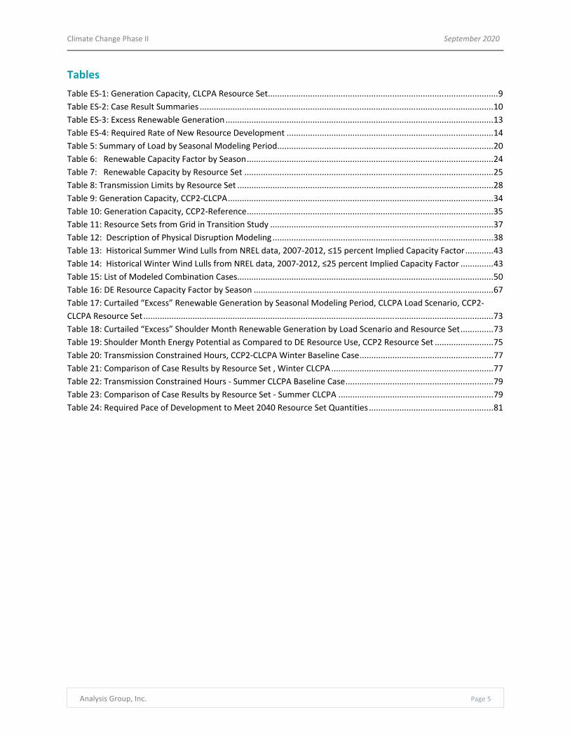
we can identify the characteristics required of the resource. In this, certain observations stand out. First, even in
the baseline cases (i.e., before layering in climate disruption events), there are periods of very low output from the
renewable resources during periods of demand when resources need to be available to meet the bulk of the
system’s annual energy requirements. During such periods, the need for the DE Resource climbs very high ‐ at
times more than 30,000 MW. This is true even though the DE Resource is not significantly utilized on an annual
energy basis, and has a very low capacity factor, at or less than ten percent. Second, the DE Resource needs to be
highly flexible ‐ it needs to be able to come on quickly, and be able to meet rapid and sustained ramps in demand.
The results in Table ES‐2 show that the minimum one‐hour ramp requirement, even in the baseline CCP2‐CLCPA
case, approaches 12 GW, and climbs to nearly 13 GW in multiple CLCPA climate disruption cases. Moreover, as can
be seen in Figure ES‐3, the ramping capability of the DE Resource is even larger when viewed across multiple
hours. For example, the four‐hour period of greatest ramp in the CCP2‐CLCPA case in the winter exceeds 20,000
MW.
Figure ES‐3: Maximum Hourly Ramping Requirement, CCP2‐CLCPA Winter Case
The assumed increase in inter‐zonal transfer capability in the CCP2 resource sets enables a renewables‐heavy
resource mix and improves reliability, but also increases vulnerability to certain climate disruption scenarios.
The CCP2 resource sets are designed to maximize the contribution of renewable resources which, due to available
land area and ease of siting, are heavily weighted towards the upstate region. As a result, it is necessary to assume
a major build out of the transmission system in New York, to enable the upstate renewable resources to contribute
‐5,000
0
5,000
10,000
15,000
20,000
25,000
30,000
35,000
40,000
Load
(MW)
Hour of the Day
Load (Average Day) Minus Renewables and Baseload (incl. Hydro, Nuclear, Imports)
Load (Max Ramp Day) Minus Renewables and Baseload (incl. Hydro, Nuclear, Imports)
Climate Change Phase II September 2020
Analysis Group, Inc. Page 13
to meeting load in the downstate region. Across the climate disruption cases, the increased transfer capability
improves the resilience of the power system to all events that are localized, such as offshore storms or wind lulls
that only affect the upstate or downstate regions, as well as to some disruptions that affect load and generation
across the state, such as heat waves and cold snaps. Conversely, the increased reliance on transmission increases
the vulnerability of the system to climate disruption events that specifically impact transmission capability,
including icing events or major storms that disable transmission capacity.
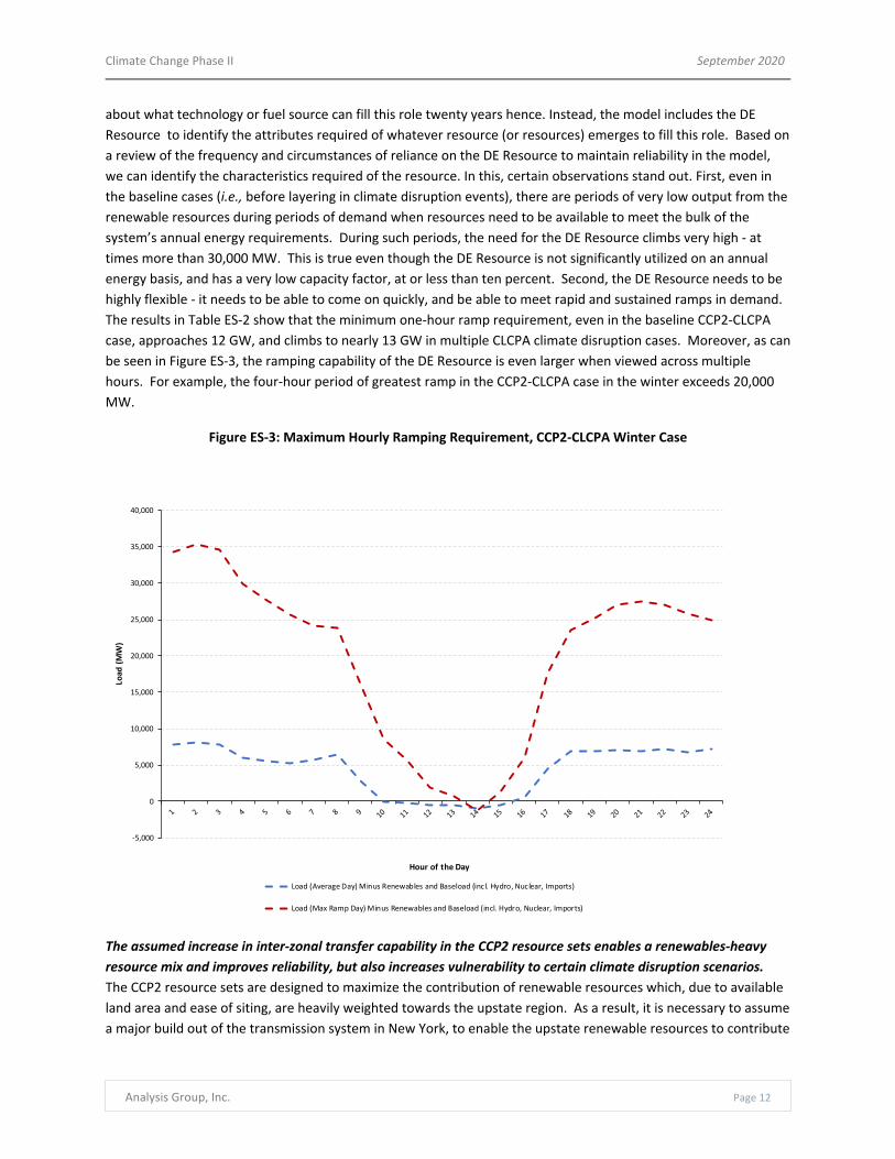
Cross‐seasonal differences in load and renewable generation could provide opportunities for renewable fuel
production. The CCP2 resource sets are constructed to be able to meet peak demand in the winter and summer
seasons based primarily on production from renewable resources. However, this means that there is a substantial
amount of renewable generation that is excess, or “spilled,” in off‐peak seasons and hours. This introduces the
potential for a seasonal storage technology to help meet the needs represented in the analysis by DE Resource
generation during the summer and winter. Such potential assumes the emergence of economic technologies
capable of converting excess renewable energy to a fuel and storing it for later use, or the development of other
long term storage technologies. For example, as seen in Table ES‐3, the excess renewable generation in the
shoulder season modeling period under the CCP2‐CLCPA case totaled roughly 23,204 GWh, while the DE Resource
use in the winter modeling period was just 4,401 GWh. This raises the possibility that, should such technologies or
capabilities emerge, excess off‐peak renewable generation could help meet the peak‐month energy requirements
represented in the model by generation from the DE Resource.
Table ES‐3: Excess Renewable Generation
The current system is heavily dependent on existing fossil‐fueled resources to maintain reliability, and
eliminating these resources from the mix will require an unprecedented level of investment in new and
replacement infrastructure, and/or the emergence of a zero‐carbon fuel source for thermal generating
resources. A power system that is effectively free of GHG emissions in 2040 cannot include the continued
operation of thermal units fueled by well‐based natural gas. However, these are the very units that are currently
vital to maintain power system reliability throughout the year. This is the fundamental challenge of the power
system transition that will take place over the next two decades. Indeed, this transition must take place at the
same time that electricity demand in the state will grow significantly if electrification of other economic sectors,
such as transportation and heating, is needed to meet the economy‐wide GHG emission reduction requirements.
In all four cases studied, the required investment in and development of renewable resources is substantial, and
far greater than anything previously experienced in New York. Table ES‐4 shows the pace of development required
for each case and resource set, compared to the historical capacity growth rate in New York.
Season
Aggregate Excess
Renewable
Generation (GWh)
Average Hourly
Excess Renewable
Generation (MW)
Average Hourly Percentage
of Excess Renewable
Generation (%)
Winter 4,401 6,112 13.66%
Summer 3,926 5,453 13.95%
Shoulder 23,204 32,227 75.80%

Climate Change Phase II September 2020
Analysis Group, Inc. Page 14
Table ES‐4: Required Rate of New Resource Development
Overall, the key reliability challenges identified in this study are associated with both how the resource mix
evolves between now and 2040 in compliance with the CLCPA, and the impact of climate change on
meteorological conditions and events that introduce additional reliability risks. The climate disruption events
modeled in the EBM may be more frequent and/or more severe than in the past, and this increases NYISO’s
challenges in managing reliability risks over time. Nevertheless, such events do not appear to be qualitatively
different than similar events experienced in the past, and present reliability challenges that may be considered
similar to those faced today. With sufficient planning and preparation such events could be managed to maintain
reliability in much the same way current weather‐based disruptions are managed. However, on top of this the
analysis demonstrates that, based on current information and technologies, the evolution of the system to one
focused on low/zero‐carbon resources and the infrastructure needed to support such a resource mix could
introduce a number of key vulnerabilities to system reliability. These challenges include the variability of the
meteorological conditions affecting renewable generation, the temporal limitations of existing battery storage
technologies, and the increased dependence on resources distant from load centers. Based on our analysis,
managing this transition seems to introduce reliability challenges that may be more difficult than those arising
from the conditions of a changing climate. Most importantly, this analysis suggests that establishing electricity
market designs and energy policies to encourage innovation and accelerate advanced energy resource
development will be key to reliably and economically managing the transition in the electric sector in New York.
Comparing the CCP2 resource sets to the GIT resource sets reveals key differences in how the system makeup in
2040 can affect reliability outcomes. There are key differences between the Climate Change Phase II resource sets
and those developed for the Grid in Transition study. First, given the different mixes of resources, the proportion
of load met by DE Resources in the CLCPA winter load scenario is roughly nine percent for the CCP2‐CLCPA
resource set, but about 20 percent for the GIT‐CLCPA resource set. In addition, given differences in the assumed
level of transmission on the system (the GIT resource set does not include any expansion of the current
transmission system), constraints on the Total East and Total South interfaces are binding in a larger percentage of
hours under the GIT resource set, which means that DE Resources downstate are dispatched to provide electricity
in more hours. The differences also lead to changes in vulnerability to climate disruptions. There are more hours
with loss of load occurrences in the state‐wide and offshore wind lull cases under the CCP2 resource sets, given the
smaller overall quantity of DE Resources and greater reliance on wind resources. Conversely, the lower level of
Nameplate Capacity (MW)
Required 2020‐2040 Capacity
Growth Rate (MW/yr)
Wind (Land‐
based and
Offshore)
Grid‐Connected
Solar
Wind (Land‐
based and
Offshore)
Grid‐Connected
Solar
Existing Resources (2020) 1,739 32
Climate Phase II Reference Case
Resource Set (2040)39,962 34,354 1,911 1,716
Climate Phase II CLCPA Scenario
Resource Set (2040)56,263 39,262 2,726 1,962
Grid in Transition Reference Case
Resource Set (2040)23,522 30,043 1,089 1,501
Grid in Transition CLCPA Scenario
Resource Set (2040)48,357 31,669 2,331 1,582
Historical Capacity Growth Rate (2011‐2020, MW/yr) 48 0

Climate Change Phase II September 2020
Analysis Group, Inc. Page 15
interzonal transfer capability in the Grid‐in‐Transition study resource set leads to more severe load losses during
scenarios that affect upstate resources, such as severe windstorm and icing events.
In this study, we provide results for two very different visions for the evolution of the power system ‐ one that
relies on renewables and transmission (the CCP2 resource sets), and one that places greater emphasis on the
backstop resource ‐ that is, the potential emergence of a zero‐carbon generation or fuel source (the GIT resource
sets). These are only two of a wide range of potential outcomes as the system and technologies change over the
next two decades, but they represent in some sense two bookends to potential system changes ‐ one focused on
aggressive system infrastructure development, and one that looks more like the current system, but is dependent
on the development of low or zero‐GHG fuel sources. The key differences between them are the relative levels of
investment in system infrastructure, and the degree of reliance on the DE Resource.
For example, if there is skepticism that an economic fuel or technology will emerge and be widely available, and
that can deliver reliable capacity, energy, reserves, and flexible operating attributes with little or no emissions of
GHGs, then the pathway may be more heavily tilted towards aggressive investment in and development of
renewable and transmission infrastructure, such as in the CCP2 resource sets. This approach would allow the
system to operate with relatively low annual generation from the DE Resource. Conversely, if such a fuel or
technology were to emerge, be technologically and economically viable, and be widely available, then there is less
need to invest the significant capital needed to build out renewable and transmission infrastructure to meet the
CLCPA requirements. These differences provide useful insight into the challenges New York State will face in
guiding and managing what will likely be a rapid transition over the next two decades.

Climate Change Phase II September 2020
Analysis Group, Inc. Page 16
II.Analytic Method
Overview of Analytic Method
Analysis Group developed and applied a multi‐step energy balance analysis to assess the risks to the reliability of
the NYISO power system posed by changes in system conditions and infrastructure due to climate change in New
York State. The analysis is completed for 2040 based upon the state’s CLCPA requirements for that year. It reflects
both the Climate Change Phase I results with respect to climate‐induced changes to system demand, and
assumptions described further in this report with respect to system infrastructure available in 2040. Figure 4
presents the structure of the analysis used to generate results for all cases, and Figure 5 summarizes the inputs
and logic of the energy balance model. Section B provides a more detailed description of the analytic method,
model components, and data and information sources used in the analysis.
Figure 4: Structure of Analysis

Climate Change Phase II September 2020
Analysis Group, Inc. Page 17
Figure 5: Energy Balance Model Steps and Data Sources

Climate Change Phase II September 2020
Analysis Group, Inc. Page 18
Framework for Energy Balance Analysis
Analysis Group’s energy balance model is a deterministic, scenario‐based assessment of system operations in a
future year ‐ 2040. The model evaluates system reliability under different combinations of load including
assumptions regarding future loads and hourly shapes based on weather. It analyzes different resource sets and
variations in future system resource mix and transmission topology. The model examines various climate
disruptions under which altered climate conditions affect load, resource availability/generation, and transmission
availability. Given that the load levels and the output of renewable generating capacity vary widely over the
course of the year, we evaluate three representative seasonal modeling periods: summer, winter, and shoulder
season. For each season we model a single month.
There are three core elements to the modeling framework ‐ (1) Load, (2) Resources, and (3) Climate Disruptions:
(1) Load: The starting point for the analysis is expected system conditions for the future year of 2040, based on
load scenarios developed by Itron in the NYISO Climate Impact Phase I study (“Phase I Study”).13 The Phase I load
scenarios reflect the impact of climate change and state policy on electricity demand in New York state. We focus
on two of the Phase I scenarios: 1) the Reference Case, which assumes average New York State temperatures will
increase at 0.7 degrees F per decade without significant load impact from state policy; and 2) the CLCPA Scenario,
which assumes the same temperature trend, but reflects load impacts from electrification of the transportation
and building sectors in the state, and enhanced implementation of energy efficiency. These factors are described
in more detail in Section II.B.1 below.
(2) Resources: The next step involves development of resource sets for each of the two load scenarios, based on
the Analysis Group Climate Change Phase II (CCP2) set and the NYISO Grid in Transition (GIT) Study set. This leads
to four resource sets: CCP2‐reference, CCP2‐CLCPA, GIT‐reference, and GIT‐CLCPA. The purpose of this step is to
position the power system to reliably meet the Phase I 2040 demand levels. The resource sets are developed to
maintain reliable system operations in the season with the highest peak load, which is summer for the Reference
Case and winter for the CLCPA scenario. For the CCP2 resource sets, the starting point for each resource set is the
2019 CARIS Phase I “70x30” case, which assumes specific quantities of renewable and nonrenewable resources by
load zone. This resource set alone is insufficient to meet demand; thus, the analysis adds renewable generating
capacity, storage capacity, transmission capability, and DE resource capacity in quantities sufficient to meet the
seasonal peak demand.14 The resource sets are described in more detail in Section III.E below.
(3) Climate Disruption Scenarios: With the Phase I load scenarios and reliable starting point resource sets in hand,
we then identify a range of impacts on loads and resources associated with the impacts of a changing climate.
These climate disruptions are used to define seasonal “cases,” which are run through the energy balance model to
identify any reliability risks associated with operations under those conditions. The results of the model identify
the magnitude, frequency and duration of any periods where available generation was potentially insufficient to
13 Itron, “New York ISO Climate Impact Study; Phase 1: Long‐Term Load Impact,” (hereafter “Phase I Study”), December 2019. 14 Analysis Group developed the reliable resource sets for use in this study. As described in Section II.F below, we also evaluate system outcomes using
the resource set assumed in the Grid in Transition study, which varies in the location and quantities of both renewable and DE resources across zones.

Climate Change Phase II September 2020
Analysis Group, Inc. Page 19
meet load over the duration of the seasonal modeling period, or where significant storage or DE resource output is
needed to supplement renewable generation.15
The sections that follow describe the methods and data used in the model and analyses. Section B addresses the
development of the load scenarios and seasonal modeling periods. Section C describes the baseline resource
assumptions that apply across all cases with respect to generation and storage resources and transmission.
Section D reviews the “dispatch” and intrastate power transfer logic that is applied in across cases. Section E
details the construction of resource sets by load scenario, and finally Section F compares the resource sets
developed for this study with those used in the Grid in Transition study.
Construction of Seasonal Modeling Periods and Load Scenarios
The model represents three 30‐day seasonal modeling periods during 2040, under two load scenarios. The
selection of these modeling periods was designed to represent normal winter peak, summer peak, and shoulder
season weather conditions, and to reflect the associated electricity demand and load shapes, and the seasonal
generation profiles of renewable resources. The analysis is a review of reliability under normal conditions; it is not
meant to represent a severe or worst case scenario. This section describes (1) the load scenarios used to represent
electrical demand and (2) the selection of the modeling periods.
1. Load Scenarios
The load profiles used in the energy balance model are derived from the NYISO Climate Impact Phase I study
conducted by Itron in 2019.16 For each day of the years from 2020 to 2050, the Phase I Study estimated daily peak
loads and total energy based on historical average daily temperatures after adjustments for the temperature
impacts of climate change, using a nonlinear model of load‐temperature response.17 In each scenario, hourly loads
were further modified with adjustments to account for predicted energy efficiency, and electrification of the
transportation and building sectors. The daily peak and energy forecasts were then combined with a forecasted
system hourly load shape to create an 8,760 hour baseline load forecast for each year.18 The Phase I Study
modeled four load scenarios: the Reference Case, the Reference Case with accelerated weather trend, the Policy
Case, and the CLCPA case.
This study focuses on two of the Phase I load scenarios, with the following underlying assumptions:
1) Reference Case
a) 0.7 degrees F per decade increase in average New York state temperatures19
b) Increases in energy efficiency
c) Increases in electric vehicle charging load
15 We do not explicitly model operating reserves in this framework. In nearly all hours, there are sufficient DE resources available in the model to cover
reserve needs in all zones across the state, and we do not model the degree of reserve drawdown as a metric in this analysis. This means that during the
limited number of hours when the energy balance model predicts loss of load in one of the combination cases modeled, additional DE resources above
those assumed would be needed to meet load and/or maintain reserves. 16 Itron, “New York ISO Climate Impact Study; Phase 1: Long‐Term Load Impact,” December 2019. 17 Phase I Study, pp. 29‐41. 18 Phase I Study, pp. 38‐41. 19 0.7 degrees F per decade is the historical trend based on weather station data from 1950 through 2018. Phase I Study, pp. 9, 16.

Climate Change Phase II September 2020
Analysis Group, Inc. Page 20
2) CLCPA Case
a) 0.7 degrees F per decade increase in average New York state temperatures
b) Increases in energy efficiency
c) Increases in electric vehicle charging load
d) Increases in residential and commercial building electrification
The CLCPA Case in the Phase I study assumed significant electrification of both the residential and commercial
building sectors.20 This electrification load comprises three components: 1) base‐use electrification, which includes
replacement of existing gas‐powered household appliances with electric‐powered models; 2) cooling
electrification, with additional summer load from cooling heat pumps and A/C units; and 3) heating electrification,
with additional winter load from electric heat pumps. Cooling and heating electrification are based on historical
hourly profiles of loads, and vary with daily temperature. The additional heating electrification load is sufficient in
the CLCPA scenario to move the system as a whole from summer‐peaking to winter‐peaking, with highest loads in
January.
The Phase I study load scenarios also account for expected growth in behind‐the‐meter solar generation, but this
study removes that impact from loads and instead treats behind‐the meter solar as a generating resource.
2. Seasonal Modeling Periods
Both loads and renewable generation vary considerably across the course of the year, and present different types
of challenges for reliability during different seasons. For example, wind capacity factors are on average highest in
winter, when solar capacity factors are lowest, and vice versa. In addition, the modeling periods needed to be long
enough to capture multi‐day or multi‐week trends in generation resource availability and output, which are
affected by natural variance in meteorological conditions over the course of a day, week, month, and season.
As a result, this study analyzes three 30‐day representative modeling periods in 2040, one for the summer season,
one for the winter season, and one for the shoulder season. The Phase I Study provided 8,760 hourly loads for all
of 2040. The Phase II Study uses the first 30 days of the months of July, January, and April for the summer, winter
and shoulder seasons. These months were selected because for each load scenario, July 2040 included the day
with the forecasted summer peak load, January 2040 included the day with the forecasted winter peak load, and
April 2040 had the lowest total energy consumed. Table 5 summarizes the load scenarios by peak and total
energy.
Table 5: Summary of Load by Seasonal Modeling Period
20 Phase I Study, pp. 46‐50.
Summer Winter Shoulder
Dates7/1/2040 ‐
7/30/2040
1/1/2040 ‐
1/30/2040
4/1/2040 ‐
4/30/2040
Peak Load (MW) 38,666 28,010 23,507
Total Energy (GWh) 19,013 14,111 11,385
Peak Load (MW) 48,589 57,144 27,060
Total Energy (GWh) 22,476 27,322 12,497
Reference
Case
CLCPA
Case

Climate Change Phase II September 2020
Analysis Group, Inc. Page 21
Construction of Resource Sets by Load Case
This section describes the construction of the CCP2 resource sets underlying the analytic model, which are the
generation and transmission inputs making up the supply side of the electrical system. Each resource set is
specifically designed to establish a reliable starting point for the analysis, given the load forecasts from the Phase I
report. With a reliable starting point, we then run scenarios that incorporate the physical disruptions associated
with climate change impacts on load and system resources.
As a starting point, the CCP2 resource set is based on the 2019 CARIS 1 Phase 1 “70X30” Case for generation
inputs, and assumes a transmission topology provided by NYISO that reflects current inter‐zonal transfer limits.
Intra‐zonal and/or local transmission limitations were not assessed in this study. The CARIS generation inputs are
designed to meet the CLCPA mandate that New York consumers be served by 70 percent renewable energy by
2030, and include significant additional development of renewable resources above current levels.
Two factors influence the resources added to get to a reliable system starting point. First, the Phase I CLCPA case
requires additional resources to meet incremental load due to both temperature‐induced demand increases, and
the assumed electrification of the transportation and building sectors. Second, the CLCPA establishes certain
requirements that may affect the resources available to meet demand in 2040. Specifically, the Act requires 100
percent of the state’s electricity supply to be emissions free by 2040,21 and the state must reach at least 85%
reduction on the way to net zero greenhouse gas emissions by 2050 across all economic sectors. This will require a
significant transformation of the existing system in ways that are not easy to anticipate at this time.
In consideration of these factors, we constructed a set of additional resources to reliably meet system demand in
2040. In doing so, we recognize that there is a vast array of different resource types and pathways to meeting the
CLCPA requirements, and potentially resources, technologies, and fuels that are currently not commercially
available. Further, even the resource options that we consider based on current information will evolve
significantly in the coming decades, and each has different properties in terms of availability and generation
profiles, maximum capacity potential, total energy potential, and cost. Thus our starting point resource set should
be viewed as but one among a vast number of potential resource combinations, technologies or pathways that
could reliably meet electricity demand in 2040.
Given the unique circumstances and focus of state law and policy in New York, the analysis developed a resource
set prioritizing the development and operation of zero‐carbon renewable resources and the expansion of high‐
voltage transmission capacity as needed to move generation to load within the state. Specifically, in order to
identify a combination that fully met load in all hours of the modeling periods, the resource set was built from the
following resources, in the following order:
1) Assume the retention of existing low‐ and zero‐carbon resources
Maintain in 2040 the availability and operation of existing hydroelectric and nuclear capacity as baseload
system resources.
2) Maximize the development of renewable generating resources in New York state
Build out solar and land‐ and offshore wind generating capability to the maximum feasible extent, based
on an evaluation of need and a review of technical potential. Steps one and two are key to addressing
aggregate incremental energy demand.
3) Increase low/zero carbon resources imported from neighboring regions
21 NY Senate Bill S6599, pp. 4, June 18, 2019.

Climate Change Phase II September 2020
Analysis Group, Inc. Page 22
The analysis assumes that it is possible to increase the transfer of low‐emission capacity and generation
from Canada through the addition of new transmission lines to the north. This resource provides
assistance with both incremental energy needs and the ability to instantaneously balance system load.
4) Mitigate the impact of electrification through demand modulation by the “shaping” of EV load
The analysis assumes that with electrification of the transportation sector, electricity markets and pricing
in New York will provide incentives for the management of demand associated with electric vehicle
charging. Such incentives will assist with managing peak demand and instantaneous power needs, but
they will not address aggregate energy deficits.
5) Enable the efficient movement of diverse generation sources across the state through additional
transmission
The vast majority of land‐based renewable resource potential is in upstate New York. A renewables‐
focused resource set will need significant increases in inter‐zonal transfer capability, helping to reduce
zonal bottlenecks.
6) Maximize the participation in markets of price responsive demand
The combination of wholesale market designs and new distributed resource initiatives and technologies
will provide incentives for significant expansion of price responsive demand, helping meet instantaneous
power needs.
7) Continue the aggressive development of energy storage technologies
The analysis assumes that current initiatives and changing economics will continue growth in the
development of storage within the state, helping address instantaneous power needs
8) Dispatchable and emissions‐free resource
Even with the substantial infrastructure and resource growth in steps 1‐7, there will likely need to be a
dispatchable resource with attributes needed to help balance the system under certain conditions, such as
high loads, loss of resources, inter‐zonal transfer limits, and limited output from variable resources. This
report focuses on the attributes needed from such resources, without assuming we can anticipate what
form they will take in 2040 as technologies continue to evolve.
As noted, the starting point CCP2 resource set represents only one possible pathway or outcome. The Grid in
Transition resource set, reviewed in Section III.E., presents another, and very different, potential pathway for the
development of resources to reliably meet 2040 system needs, one focused more on a DE resource, and less on
renewables and transmission. In reality, it is likely that the manner in which the system evolves to meet the
changing nature of electricity demand and resource requirements will involve some elements of both resource
sets, but will not look exactly like either. Nonetheless, the results, and how they differ across these two resource
sets, offer interesting insights into the challenges that will need to be addressed through market design,
resource/technological development, and policy in the coming decades.
In the following sections, we describe in more detail our assumptions with respect to each of the categories of
resources described above for the CCP2 resource sets.
1. Retention of Baseload Resources
The generation fleet used in the energy balance model assumes the continued operation of a number of baseload
hydroelectric and nuclear units. Resource retirements are guided by 2019 CARIS Phase 1 “70X30” Case. CARIS
performs a sensitivity to examine the impact of upstate nuclear operations beyond the currently regulated Zero
Emission Credits (“ZECs”) eligibility criteria.22 This resource set assumption affects the operation of Nine Mile Point
22 NYISO, “2019 CARIS 1 70X30 Scenario Development”, pp. 12, September 6, 2019.

Climate Change Phase II September 2020
Analysis Group, Inc. Page 23
1 & 2, James A. Fitzpatrick 1 and R.E. Ginna 1 in operation. We assume the plants will operate at a 100 percent
capacity factor for all hours of the thirty day modeling period. Actual resource operations across the full year will
be lower, based upon the dependable maximum net capability and forced outage rates of the nuclear resources in
the future.
CARIS assumes that the majority of the existing hydro resources will continue in operation. Each resource set
maintain 913 MW of run of river hydro and 3,573 MW of pondage hydro. The hourly capacity factor of run‐of‐river
hydro units is based on historical 2018 generation data.23 The Niagara pondage units (Robert Moses and Lewiston)
operate on a daily cycle that depends on season and load case. Niagara operations obey water levels set by an
international water treaty and are synchronized with solar generation to generate in hours when need is greatest.
The other hydro pondage units, including the St. Lawrence‐Franklin D. Roosevelt unit, are assumed to operate at a
100 percent capacity factor for all hours of the modeling period. The Gilboa pumped storage unit behaves as a
storage resource and is described in Section II.C.7. Additional baseload nuclear and hydroelectric resources are not
included in the resource set.
2. Renewable Resources (CARIS Starting Point)
The model includes four types of renewable resources: land‐based wind, offshore wind, utility‐scale solar, and
behind‐the‐meter solar. The starting point for the amount of wind and solar resources modeled is the nameplate
capacity of these resources assumed in the 2019 CARIS Phase I study as of February 2020.24 The 2019 CARIS Phase I
CLCPA case starting point assumes an additional 17,761 MW of wind and 25,070 MW of solar, and aligns with
renewable targets established in state policies, including 9,000 MW of offshore wind by 2035 and 6,000 MW of
behind the meter solar capacity by 2025.25 Solar and wind resources are distributed according to capacity shares
by zone from the 2017 and 2018 CES REC solicitation awards and the interconnection queue.26 The study does not
assume any utility solar in Zones G, H, I, and J, in consideration of potential siting challenges and land costs.
Similarly, no land‐based wind is assumed in Zones F through K.
The generation profile, in terms of hourly capacity factors, assumed for the solar units are based on 2006 data
from the NREL Solar Power database using 62 simulated solar farm sites across New York State.27 Two Zones did
not have solar farm data. For Zone D BTM solar, a simple average of bordering Zones F and E was used. For Zone K
utility solar, the BTM solar data from Zone K was uprated by the average ratio of utility to BTM solar NYCA‐wide.
The hourly capacity factors assumed for the wind units are based on 2009 data at simulated 100 meter turbine
height from the NREL's Wind Toolkit Database, using 721 weather sites in NY.28 A summary of renewable resource
capacity factors by season is listed in Table 6. As shown, solar capacity factors are higher on average in the
summer modeling period than in the winter, and wind capacity factors are higher on average in the winter than in
the summer.
23 Aggregated Run of River Hydro Production Data collected from NYISO’s Decision Support System. 24 The 2019 CARIS Phase I study was ongoing at the time this study was conducted, and certain assumptions in the CARIS Phase I Study have been altered
since February 2020. 25 The CARIS starting point assumes 6,750 DC MW in behind‐the‐meter solar capacity in 2040 in the CLCPA case, which translates to 5,439 AC MW. For
the purposes of this study, we use the AC MW as the basis for nameplate capacity of solar resources. This is a larger nameplate capacity for behind‐the‐
meter solar in the CLCPA case as compared to the Reference case (3,629 AC MW). 26 NYISO, “2019 CARIS 1 70X30 Scenario Development,” pp. 15, September 6, 2019. 27 NREL Solar Power Database, https://www.nrel.gov/grid/solar‐power‐data.html. 28 NREL Wind Toolkit Database, https://www.nrel.gov/grid/wind‐toolkit.html.

Climate Change Phase II September 2020
Analysis Group, Inc. Page 24
Table 6: Renewable Capacity Factor by Season
Notes: [1] Wind capacity factors are based on 2009 historical data; solar capacity factors are based on 2006 historical data Sources: [1] NREL Solar Power Database, https://www.nrel.gov/grid/solar‐power‐data.html. [2] NREL Wind Toolkit Database, https://www.nrel.gov/grid/wind‐toolkit.html.
3. Renewable Resource: Additions to 2040
As noted, the approach used in developing the resource set assumes that renewable resources will be prioritized
for development to help meet the CLCPA 100 percent renewable resources requirement for 2040. This means that
a significant quantity of new renewable resources needs to be added in the model, above and beyond the 2019
CARIS starting point resources, in order to meet electrical loads in that year. Due to seasonal differences in
capacity factors among renewable resource types, the optimal mix of renewable resources depends in part on
characteristics of the load scenarios. For example, wind resources are more productive in winter months and
therefore can generate more than solar resources of the same nameplate capacity, to ensure reliability in a winter‐
load‐peaking scenario. On the other hand, in a summer‐load‐peaking scenario, additional solar resources may be
more useful in meeting energy needs.
To capture these seasonal effects, additional renewable resources were added to the resource sets using an
iterative marginal benefit analysis targeted at the seasonal modeling period with the greatest load for each
scenario. These are the summer period for the reference scenario, and the winter period for the CLCPA scenario.
Starting from the CARIS starting point resource set, the nameplate capacity of wind and solar resources were each
increased in specific increments of 25 percent of the CARIS starting point quantities. In each iteration, we added
whichever technology type (either wind or solar) reduced the aggregate energy deficit the most. This process
continued iteratively until the total energy deficit for the peak month was met. In addition, the total nameplate
capacity for each resource type was not allowed to exceed an estimate of its technical potential in New York State
(see Appendix A.3 for more details). This technical potential upper limit was reached in the CLCPA case for both
land‐based and offshore wind. The results of the marginal benefit analysis for each resource set can be found in
Table 7.
Average Capacity Factor by Season
Resource Type Summer Winter Shoulder
Wind (Land‐based) 27.31% 46.22% 51.72%
Wind (Offshore) 30.14% 47.81% 58.42%
Solar (Behind‐the‐meter) 17.98% 8.02% 18.20%
Solar (Grid‐Connected) 20.23% 8.61% 20.25%

Climate Change Phase II September 2020
Analysis Group, Inc. Page 25
Table 7: Renewable Capacity by Resource Set
Notes: [1] Technical Potential for land‐based wind in New York is estimated by NREL to be 35,200 MW. [2] Technical Potential for offshore wind is 21,063 MW calculated from BOEM and DOE data assumes maximum 3 MW/km2 wind capacity installed in the 7,021 km2 New York Bight Lease Areas. Sources: [1] NREL, Estimating Renewable Energy Economic Potential in the United States: Methodology and Initial Results, August 2016, Appendices A and F. [2] Bureau of Ocean Energy Management, New York Bight, available at https://www.boem.gov/renewable‐energy/state‐activities/new‐york‐bight. [3] Department of Energy, Computing America’s Offshore Wind Energy Potential, September 9, 2016.
4. Imports from Neighboring Areas
Our analysis assumes fixed quantities of zero‐carbon imports during the modeling period, but no other imports or
exports into or out of New York.29 Based on NYISO data on current import flows, a baseline level of 1,500 MW of
imports into Zone D were assumed in each hour, and an additional 1,310 MW of imports in 2040 associated with a
potential increase in imports through the development of additional transmission infrastructure. The assumed
flows for imports are represented in Figure 6.
29 The analysis assumes that New York’s requirement for a GHG‐emission free electric system in 2040 extends to imported power, and does not assume
that neighboring U.S. regions will meet these requirements. Thus, for the purpose of this modeling exercise, the study does not assume any
imports/exports between New York and neighboring U.S. regions. However, there are low/zero‐emission resources available and potentially available in
neighboring Canada, and there is interest in importing certifiable zero‐carbon hydro resources if or as available. Thus, for the model assumes the
availability in 2040 of energy and capacity imports from Canada.
Technology Type A B C D E F G H I J K Total % Increase
CARIS Starting Point
Land‐Based Wind 2,692 390 1,923 1,935 1,821 ‐ ‐ ‐ ‐ ‐ ‐ 8,761 ‐
Offshore Wind ‐ ‐ ‐ ‐ ‐ ‐ ‐ ‐ ‐ 6,391 2,609 9,000 ‐
BTM Solar (CLCPA) 704 218 596 69 673 827 684 61 90 672 846 5,439 ‐
BTM Solar (Reference) 470 146 398 46 449 552 456 40 60 448 565 3,629 ‐
Grid‐Connected Solar 5,748 656 3,585 ‐ 2,268 4,661 2,636 ‐ ‐ ‐ 77 19,631 ‐
CCP2 ‐ Reference Case
Land‐Based Wind 6,057 878 4,327 4,354 4,097 ‐ ‐ ‐ ‐ ‐ ‐ 19,712 125%
Offshore Wind ‐ ‐ ‐ ‐ ‐ ‐ ‐ ‐ ‐ 14,380 5,870 20,250 125%
BTM Solar 822 255 696 81 786 965 798 71 105 784 988 6,351 75%
Grid‐Connected Solar 10,059 1,148 6,274 ‐ 3,969 8,157 4,613 ‐ ‐ ‐ 135 34,354 75%
CCP2 ‐ CLCPA Case
Land‐Based Wind 10,816 1,567 7,726 7,774 7,316 ‐ ‐ ‐ ‐ ‐ ‐ 35,200 302%
Offshore Wind ‐ ‐ ‐ ‐ ‐ ‐ ‐ ‐ ‐ 14,958 6,105 21,063 134%
BTM Solar 1,409 436 1,193 138 1,345 1,653 1,367 121 179 1,343 1,692 10,878 100%
Grid‐Connected Solar 11,496 1,312 7,170 ‐ 4,536 9,322 5,272 ‐ ‐ ‐ 154 39,262 100%
Zone

Climate Change Phase II September 2020
Analysis Group, Inc. Page 26
Figure 6: Imports During Modeling Period
5. Modulation of EV Load Shape
The potential increase in electric vehicles and the transition of the electric generation sector to heavy reliance on
renewable resources provides incentives and opportunities for efficient shifts in load over the course of a day. In
particular, the daily load shape for electric vehicle charging demand set in the Phase I Study assumes a charging
peak in the evening, around hour 20 (see Figure 7 below). However, a shift to a “flatter” load shape that is more
equal across evening hours and/or all hours of the day could help reduce peak demand and better tailor the timing
of demand to the pattern of generation from renewable resources.
The study models load management based on the NYSERDA report, Electricity Pricing Strategies to Reduce Grid
Impacts from Plug‐in Electric Vehicle Charging in New York State. That report shows that use of a time of use (TOU)
rate could significantly shift the timing of daily peak EV load from evening hours to early morning hours.30 A TOU
rate varies the cost of electricity depending on the time of day, with higher rates during peak load hours and lower
rates during off‐peak hours. A TOU rate acts as an incentive for an EV owner to delay the start of charging to
30 NYSERDA, “Electricity Pricing Strategies to Reduce Grid Impacts from Plug‐in Electric Vehicle Charging in New York State”, June 2015
https://www.nyserda.ny.gov/‐/media/Files/Publications/Research/Transportation/EV‐Pricing.pdf
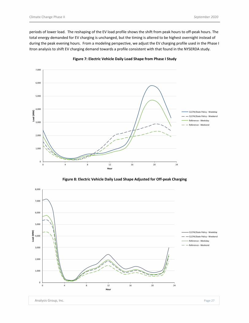
Climate Change Phase II September 2020
Analysis Group, Inc. Page 27
periods of lower load. The reshaping of the EV load profile shows the shift from peak hours to off‐peak hours. The
total energy demanded for EV charging is unchanged, but the timing is altered to be highest overnight instead of
during the peak evening hours. From a modeling perspective, we adjust the EV charging profile used in the Phase I
Itron analysis to shift EV charging demand towards a profile consistent with that found in the NYSERDA study.
Figure 7: Electric Vehicle Daily Load Shape from Phase I Study
Figure 8: Electric Vehicle Daily Load Shape Adjusted for Off‐peak Charging
0
1,000
2,000
3,000
4,000
5,000
6,000
7,000
0 4 8 12 16 20 24
Load
(MW)
Hour
CLCPA/State Policy ‐ Weekday
CLCPA/State Policy ‐ Weekend
Reference ‐ Weekday
Reference ‐ Weekend
0
1,000
2,000
3,000
4,000
5,000
6,000
7,000
8,000
0 4 8 12 16 20 24
Load
(MW)
Hour
CLCPA/State Policy ‐ Weekday
CLCPA/State Policy ‐ Weekend
Reference ‐ Weekday
Reference ‐ Weekend

Climate Change Phase II September 2020
Analysis Group, Inc. Page 28
6. Increase in Inter‐zonal Transfer Capability
In order to capture geographic constraints on electrical generation and transmission, the model applies a simplified version of the NYISO transmission network. NYISO divides the state into 11 geographic load zones, A through K, which are individually modeled in this study. The energy balance model uses a set of transmission transfer limits for each interface between load zones. The starting point for these limits is based on an N‐1
contingency analysis, as provided by NYISO (see
Figure 9). The Western New York and AC Public Policy Transmission upgrades are assumed to be in‐service.
Importantly, the distribution of renewable resources across New York is heavily weighted to the upstate region,
given the constraints on land availability and cost discussed previously. As a result, the addition of renewable
resources across New York in the amounts we assume requires substantial increases in inter‐zonal transfer
capability to allow for sufficient flows to meet zonal demand. The starting point transfer limits restrict renewable
resources’ ability to help address zonal hourly load deficits due to congestion. In the CLCPA Winter modeling
period, current transfer limits would result in an average of 3,565 MW of renewable power in each hour unable to
help meet load requirements (this is equivalent to 9.4 percent of total NYCA load).
For each transmission interface between Zones, the model assumes an increase in transfer capability by calculating
the transmission limits required to alleviate load losses in 90 percent of transmission‐constrained hours. The
results of the transmission analysis for each resource set can be found in Table 8.
Table 8: Transmission Limits by Resource Set
Interface
NYISO Limits
(Starting Point)
90% Limits
(CCP2 ‐ Reference)
90% Limits
(CCP2 ‐ CLCPA)
A to B 1,800 MW 5,133 MW 7,149 MW
C to B 1,600 MW 1,600 MW 3,319 MW
C to E 4,925 MW 8,432 MW 11,357 MW
D to E 2,550 MW 4,161 MW 6,448 MW
E to G 1,900 MW 9,279 MW 13,932 MW
G to H 7,250 MW 14,713 MW 15,791 MW
I to J 3,900 MW 8,675 MW 10,585 MW
I to K 1,200 MW 4,520 MW 5,137 MW

Climate Change Phase II September 2020
Analysis Group, Inc. Page 29
Figure 9: Simplified Transmission Map and Limits (Starting Point)
7. Energy Storage Resources
Renewable resources are dependent on variable meteorological conditions, and thus their generating output does
not always coincide with load. Energy storage allows for time shifting of generation to meet the timing of demand.
The starting point for storage resources used in our model is based on the 2019 CARIS Phase I “70x30” case. The
starting point assumes 3,900 MW of battery energy storage and aligns with the specific CLCPA target of 3,000 MW

Climate Change Phase II September 2020
Analysis Group, Inc. Page 30
by 2030.31 The battery energy storage units are assumed to have eight hours of storage duration and operate with
a 85 percent round trip efficiency.32 It also assumes that the Gilboa hydro pumped storage unit is operating
effectively as a single large battery contributing an additional 1,170 MW of storage capacity. The Gilboa unit
assumes 12 hours of storage duration and operates with a 75 percent round trip efficiency.33 The storage units
only charge when there is excess renewable generation.34
For the Reference and CLCPA cases, additional battery energy storage resources above the amounts modeled in
CARIS were added to meet instantaneous power needs. The analysis assumes a doubling of the 2019 CARIS
capacity for the Reference case (adding 3,900 MW), and quadrupling of the CARIS capacity for the CLCPA case
(adding 11,700 MW). The additional capacity is distributed geographically proportional to the total quantity of
“excess” renewable generation in the peak month. That is, batteries were distributed across zones based on the
potential to reduce the curtailment or “spilling” of renewable generation in each zone.
From a practical standpoint, the location of energy storage based on the available level of renewable generation
improves the use of transmission over the course of a day. On days with high renewable generation upstate, solar
and wind power is transmitted over lines from upstate to downstate during the daytime, while simultaneously
charging energy storage devices upstate with “excess” energy ‐ that is, energy produced in excess of available
transfer capability. In the evening and night, once solar power has dropped to zero, the storage discharges and
moves power from upstate to downstate over the same transmission lines. The location of the battery resources
for each case is shown in Figure 10 and Figure 11.
31 NY Senate Bill S6599S, pp. 9, June 18, 2019. 32 Roundtrip efficiency of less than 100 percent implies that the units do not receive their full capacity of energy inflow when charging; therefore a
battery with 8 hours of stored energy takes longer than 8 hours to charge. 33 Dames and Moore, “An Assessment of Hydroelectric Pumped Storage”, November 1981, pp.99. 34 In effect, this means that the model does not allow the DE generating technology to charge energy storage devices. As described below, we position
the DE resource to operate if and only if it is needed to avoid loss of load.
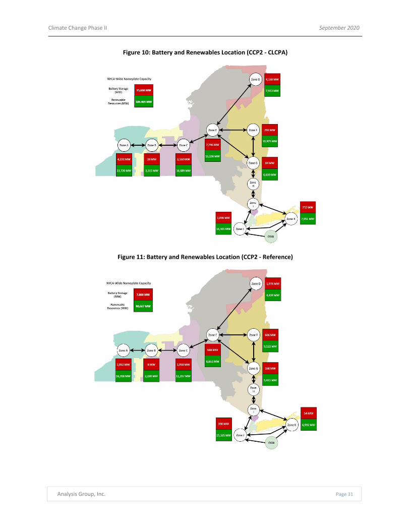
Climate Change Phase II September 2020
Analysis Group, Inc. Page 31
Figure 10: Battery and Renewables Location (CCP2 ‐ CLCPA)
Figure 11: Battery and Renewables Location (CCP2 ‐ Reference)

Climate Change Phase II September 2020
Analysis Group, Inc. Page 32
8. Price Responsive Demand
Given the nature of the transition in energy supply and use in New York over the coming decades, the study
assumes a significant expansion of price responsive demand (PRD) resources by the modeling year, 2040. The PRD
resources used in the energy balance model are based on NYISO’s Special Case Resource (SCR) Program and are
assumed to be dispatchable by NYISO.35 The starting point aligns with the 2019 summer and winter capacities from
the 2019 NYISO Gold Book, 1,309 MW in the summer capability period and 853 in the winter for NYCA.36
Specifically, the study projects a quadrupling of the current levels by 2040 for the CLCPA case, and doubling the
current levels by 2040 for the Reference Case. This results in 5,236 MW in the summer for the CLCPA case and
2,618 MW for the Reference Case, and, for the winter, 1,706 MW for the CLCPA case and 3,412 MW for the
Reference Case.
9. Dispatchable and Emissions‐Free Resource
The primary focus of our analysis is an evaluation of the potential impacts of a changing climate on power system
operations, through (1) broad‐based changes in load and supply/delivery infrastructure operations from changes in
average temperature; and (2) episodic severe weather events that are expected to increase in probability or
severity with the changing climate. Thus, our starting point in 2040 incorporates the Phase I impacts to electricity
demand of average annual changes in temperature. The study further starts with a system load and resource mix
that is consistent with current technology and policy trends. In this respect, the CLPCA has two major influences:
First, the economy‐wide focus of the Act means that the starting point should include load adjustments for
electrification of the building and transportation sectors. In the CLCPA case, this adjustment is built into the 2040
load forecast Second, to comply with the CLCPA, the study assumes that little or no fossil fuels that have positive
net GHG emissions in operation may be included in the resource set.
This latter point raises a number of challenges for the development of a “starting point” resource set. As
highlighted in Analysis Group’s Fuel Security Study, New York is highly dependent on the availability and operation
of thermal, dual‐fuel (e.g., natural gas and oil) generating resources in the downstate region to maintain reliability
generally, and in particular in cold weather conditions.37 In order to reduce or eliminate the need for generation
from these carbon‐emitting generators, the study removes them from the resource mix and supplant them with
renewables, storage, demand response, and transmission, as described above. In particular, there is substantial
“overbuild” of renewable resource capacity and increases in transfer capability in order to start with a system
where peak annual demand in the Reference and CLCPA cases is met with zero‐carbon resources. However, even
with all these additions, the variability of renewable resource output leads to circumstances where, for both the
Reference and CLCPA cases, there are periods of time that our resource mix is insufficient to meet load in all
Zones. For these reasons, a DE resource is included to fill in the gap.
The analysis does not identify exactly what the resource is. It could be thermal generating resources that looks like
the combustion turbines in operation today, but operating on a fuel that is at least net zero from a GHG emission
perspective, such as turbines running on renewable natural gas or hydrogen. It could be some form of demand
response. It could represent the emergence of a long‐term economic storage technology. Or, of course, some
35 SCRs are interruptible load customers whose load curtailments are activated by NYISO, and are part of NYISO’s Reliability‐Based Programs. NYISO,
“Demand Response,” https://www.nyiso.com/demand‐response 36 NYISO, “2019 Load & Capacity Data Gold Book,” https://www.nyiso.com/documents/20142/2226333/2019‐Gold‐Book‐Final‐Public.pdf/ 37 Paul J. Hibbard and Charles Wu, Fuel and Energy Security in New York State, November 2019.

Climate Change Phase II September 2020
Analysis Group, Inc. Page 33
combination of all of the above. There is no way to know how advances in power system technologies, costs,
policies, and consumer behavior can change the way the system meets demand twenty years hence.
Thus, the purpose of the DE resource is twofold. First, by seeing when the DE resource is relied on, it helps identify
the magnitude of the resource gap created by relying primarily on variable renewable generating resources to
meet annual, state‐wide energy needs. Second, the “operation” of the DE resource in the model defines the
attributes needed from resources that meet this gap, in terms of when it is needed, in what zones, under what
conditions, and with which system reliability attributes, such as cycling and ramping capabilities.
The DE resources are assumed to meet any remaining instantaneous power needs in the modeling period. They
are modeled as able to dispatch on demand without any operational or duration restrictions. The quantity of
capacity assumed in each resource set is calibrated to meet all remaining zonal load losses in the peak seasonal
modeling period after all other resources have been exhausted. In the Reference Case, 17,059 MW is assumed to
be available and operational in order to meet zonal load need in every hour of the summer modeling period. From
a modeling perspective, the DE resource is zonally distributed proportional to the 2017 existing thermal capacity
that fills a similar need. In the CLCPA case, 32,137 MW of DE resource availability is required to meet load in every
hour of the winter modeling period. Of this quantity, 22,471 MW is placed in the same Zones as existing thermal
capacity. The remaining DE capability is located strategically based on observed transmission bottlenecks and zonal
load loss outcomes: 539 MW is located in Zone B, 3,409 MW in Zone G, 29 MW in Zone H, 4,258 MW in Zone J, and
1,431 MW in Zone K.
The climate disruption cases, described in Section IV, involve circumstances and events that increase demand
and/or reduce or eliminate the availability of renewable resources and transmission infrastructure. These cases, in
some instances, did result is loss of load occurrences.

Climate Change Phase II September 2020
Analysis Group, Inc. Page 34
10. Resource Set Summaries
Table 9: Generation Capacity, CCP2‐CLCPA
Figure 12: Simplified Transmission Map and Limits, CCP2‐CLCPA
Nameplate Capacity by Zone, MW A B C D E F G H I J K Total
Land-based Wind 10,815.9 1,566.9 7,726.2 7,774.5 7,316.4 - - - - - - 35,200.0 Offshore Wind - - - - - - - - - 14,957.8 6,105.2 21,063.0 Solar (Behind-the-meter) 1,408.5 436.4 1,192.8 138.2 1,345.5 1,653.4 1,367.3 121.2 179.4 1,343.1 1,692.2 10,877.8 Solar (Grid Connected) 11,496.0 1,312.0 7,170.0 - 4,536.0 9,322.0 5,272.0 - - - 154.0 39,262.0 Hydro Pondage 2,675.0 - - 856.0 - - 41.6 - - - - 3,572.6 Hydro Pumped Storage - - - - - 1,170.0 - - - - - 1,170.0 Hydro Run-of-River 4.7 63.7 70.4 58.8 376.2 282.5 57.1 - - - - 913.4 Nuclear - 581.7 2,782.5 - - - - - - - - 3,364.2 Imports - - - 1,500.0 - - - - - 1,310.0 - 2,810.0 Storage 4,232.0 20.0 3,160.0 4,168.0 2,296.0 292.0 84.0 - - 1,096.0 252.0 15,600.0 Price Responsive Demand (Summer) 949.9 205.2 510.1 357.7 211.1 433.9 246.3 58.6 134.9 1,940.8 187.6 5,236.0 Price Responsive Demand (Winter) 619.0 133.7 332.4 233.1 137.5 282.7 160.5 38.2 87.9 1,264.7 122.3 3,412.0 DE Resources 465.4 674.2 1,513.4 370.0 312.7 3,390.4 6,887.2 79.8 - 11,848.1 6,595.4 32,136.6

Climate Change Phase II September 2020
Analysis Group, Inc. Page 35
Table 10: Generation Capacity, CCP2‐Reference
Figure 13: Simplified Transmission Map and Limits, CCP2‐Reference
Nameplate Capacity by Zone, MW A B C D E F G H I J K Total
Land-based Wind 6,057.0 877.5 4,326.8 4,353.8 4,097.3 - - - - - - 19,712.3 Offshore Wind - - - - - - - - - 14,380.4 5,869.6 20,250.0 Solar (Behind-the-meter) 822.3 254.8 696.4 80.7 785.5 965.3 798.3 70.8 104.7 784.1 987.9 6,350.7 Solar (Grid Connected) 10,059.0 1,148.0 6,273.8 - 3,969.0 8,156.8 4,613.0 - - - 134.8 34,354.3 Hydro Pondage 2,675.0 - - 856.0 - - 41.6 - - - - 3,572.6 Hydro Pumped Storage - - - - - 1,170.0 - - - - - 1,170.0 Hydro Run-of-River 4.7 63.7 70.4 58.8 376.2 282.5 57.1 - - - - 913.4 Nuclear - 581.7 2,782.5 - - - - - - - - 3,364.2 Imports - - - 1,500.0 - - - - - 1,310.0 - 2,810.0 Storage 1,952.0 8.0 1,958.0 1,976.0 688.0 606.0 168.0 - - 390.0 54.0 7,800.0 Price Responsive Demand (Summer) 474.9 102.6 255.1 178.8 105.5 216.9 123.1 29.3 67.4 970.4 93.8 2,618.0 Price Responsive Demand (Winter) 309.5 66.9 166.2 116.5 68.8 141.4 80.2 19.1 43.9 632.3 61.1 1,706.0 DE Resources 353.3 102.6 1,148.9 280.9 237.4 2,573.9 2,640.7 38.8 - 5,761.7 3,920.7 17,059.0

Climate Change Phase II September 2020
Analysis Group, Inc. Page 36
Representation of Electric System Operations
1. Transfer and Dispatch Logic
Electrical transfers and generation across New York were modeled using the 11‐region transmission framework
discussed in Section III.C.6. The electric system model is designed to meet load needs using available resources
subject to transmission and operational constraints.38 The model operates pursuant to a sequence of resource
loading steps, subject to the transfer constraints.
First, hydroelectric and nuclear units are assumed to generate at fixed capacity factors based on historical averages
and do not respond to load (see Section III.C.1). Next, renewable generation is dispatched in each region and then
transferred throughout the state to maximize load served through the operation of system renewable resources.
Solar and land‐based wind units are assumed to generate based on hourly profiles used in the 2019 CARIS Phase 1
70x30 Scenario (see Section III.C.2). Load within each region is served by renewable generation in that region first,
followed by inter‐region transfers to distribute regional generation surpluses across the state. Any excess
renewable generation in a given hour is used to charge storage units if there is sufficient storage headroom. The
backup resource is not used to charge storage.
In the next step of the model, if any zonal generation deficits remain, batteries and PRD are dispatched, and power
flows between Zones as needed based on load deficit severity, transmission headroom, and available stored
energy.39 If a zonal deficit is not filled by running PRD and batteries within that zone, PRD and batteries in other
Zones are transferred to the zone with a deficit, until all deficits are filled.
2. Use of Dispatchable and Emissions‐Free Resources
The final mechanism relied upon to meet load is the DE resource, which is dispatched in hours when the
combination of baseload resources, renewable generation, inter‐zonal transfers, batteries, and PRD is insufficient
to meet demand. If there is sufficient headroom on transmission lines, power generated by DE resources are
transferred to Zones with generation deficits.
Comparisons with Grid in Transition Resource Sets
In addition to the resource sets developed as described in Section III.C, this study also modeled two resource sets
developed for the NYISO Grid in Transition (GIT) study,40 which seeks to understand the reliability and market
implications of the State’s plans to transition to clean energy sources.41 The GIT resource set is based on an
economic simulation of the NYISO markets through 2040, in consideration of NYISO market operations and
economic retirement/additions of capacity. The simulation was run with the GIT resource set for both the
Reference Case and CLCPA load scenarios, without any increase in transmission transfer capability in the base
38 Note, however, that the analysis is not a production cost model which takes prices into account for unit dispatch. 39 When PRD is dispatched, the entire PRD capacity is used in each zone where there is a deficit, mimicking how the current SCR program currently
functions. 40 New York’s Evolution to a Zero Emission Power System, June 22, 2020,
https://www.nyiso.com/documents/20142/13245925/Brattle%20New%20York%20Electric%20Grid%20Evolution%20Study%20‐
%20June%202020.pdf/69397029‐ffed‐6fa9‐cff8‐c49240eb6f9d. 41 The Brattle Group, “NYISO Grid in Transition Study: Detailed Assumptions and Modeling Description,” March 30, 2020.

Climate Change Phase II September 2020
Analysis Group, Inc. Page 37
case.42 This provides a good bookend between the two resource sets where the CCP2 resource set developed
under this study looks at significant increases in transmission, while the Grid‐in‐Transition resource set has no
increase in transmission. This difference is transmission capability has a significant impact on where future
renewable resources would be located.
For comparison purposes, relative to the renewables‐focused resource set, the study tests the GIT resource set
under both the reference and CLCPA load scenarios as alternative inputs into the energy balance model. As seen
in Table 11, the Grid in Transition resource sets includes a much larger quantity of the backup resource, and lower
quantity of renewable resources, to meet total energy needs.43 In addition, the renewable resources in the GIT
resource set are located primarily in the eastern half of the state, whereas the renewables included in the resource
sets used in this study are more evenly spread across the state (For example, a large amount of solar generation is
assumed in Zone F in the GIT resource set). Finally, to provide a reliable starting point for the physical disruption
analyses, AG added additional DE resources to the resource sets to meet load in all hours of the modeling periods.
Table 11: Resource Sets from Grid in Transition Study
42 Additional alternative scenarios were included in the NYISO Grid in Transition study but were not included in this analysis. 43 The backup resource is described in the GIT study as renewable natural gas dispatchable capacity, which is used as a proxy for potential future zero
emission technology development. The Brattle Group, “NYISO Grid in Transition Study: Detailed Assumptions and Modeling Description,” March 30,
2020, slide 36.
Grid in Transition Reference CaseNameplate Capacity by Zone, MW A-E F G-I J K Total
Land-based Wind 9,754.8 0.0 0.0 - - 9,754.8 Offshore Wind - - - 9,173.5 4,593.8 13,767.3 Solar (Behind-the-meter) 452.1 2,606.7 265.0 779.9 2,009.4 6,113.1 Solar (Grid Connected) 4,771.7 20,838.5 4,376.0 - 56.4 30,042.6 Hydro Pondage + Run-of-River 4,431.7 485.6 100.7 - - 5,018.0 Hydro Pumped Storage - 1,171.3 - - - 1,171.3 Nuclear 2,095.9 - - - - 2,095.9 Imports 1,100.0 - - - - 1,100.0 Storage 1,973.5 3,276.9 895.4 2,645.5 1,945.0 10,736.3 Price Responsive Demand (SCR/EDRP) 1,054.9 216.3 318.5 938.0 634.9 3,162.6 Renewable Natural Gas Dispatchable 2,333.7 3,040.7 3,847.2 6,388.1 5,008.7 20,618.4 DE Resources (added by AG) - - - 1,283.0 797 2,080.0
Grid in Transition CLCPA CaseNameplate Capacity by Zone, MW A-E F G-I J K Total
Land-based Wind 23,254.8 0.0 0.0 - - 23,254.9 Offshore Wind - - - 17,938.0 7,164.1 25,102.2 Solar (Behind-the-meter) 537.5 2,843.1 265.0 779.9 2,009.4 6,434.9 Solar (Grid Connected) 4,907.1 21,378.9 5,326.8 - 56.4 31,669.3 Hydro Pondage + Run-of-River 4,431.7 485.6 100.7 - - 5,018.0 Hydro Pumped Storage - 1,171.3 - - - 1,171.3 Nuclear 2,156.4 - - - - 2,156.4 Imports 1,100.0 - - - - 1,100.0 Storage 5,894.2 3,014.9 260.1 2,620.7 2,317.0 14,106.9 Price Responsive Demand (SCR/EDRP) 1,462.9 306.2 472.5 1,348.9 909.1 4,499.5 Renewable Natural Gas Dispatchable 2,483.6 9,048.6 5,596.7 10,187.0 6,386.5 33,702.3 DE Resources (added by AG) 219.0 - - 3,629.0 1,988.0 5,836.0

Climate Change Phase II September 2020
Analysis Group, Inc. Page 38
IV. Cases Analyzed: Combinations of Load Scenarios and Physical
Disruptions
In order to test the resilience of the electrical system to different possible system conditions during future events,
a number of potential “physical disruptions” were modeled, representing possible future effects of climate change
on electricity demand and system infrastructure operations. The physical disruptions listed in Table 12 are
primarily intended to simulate possible short‐term adverse events with load, generation, and transmission impacts
that coincide within the modeling period. The load scenarios, resource sets, and physical disruptions are combined
into a series of cases, the results of which are evaluated through the AG system model. The sections that follow
explain the modeled impacts for each physical disruption.
Table 12: Description of Physical Disruption Modeling
Physical Disruptions: Interruptions of Resources and Transmission
1. Temperature Waves
Periods of extreme heat or cold can have contemporaneous impacts on the bulk electric system due to increased
load, changes in wind and solar generation, and impacts on transmission capacity. The temperature wave
scenarios stress the power system would be under with several days of severe temperatures across New York
State.
ID Event
Baseline None
A Heat Wave
B Cold Wave
Summer Winter
C Wind Lull ‐ Upstate Wind Generation ‐ 15% Average Capacity Factor in
Zones A‐E for 12 days
Wind Generation ‐ 25% Average Capacity Factor in
Zones A‐E for 7 days
D Wind Lull ‐ Off‐Shore Wind Generation ‐ 15% Average Capacity Factor in
Zones J‐K for 12 days
Wind Generation ‐ 25% Average Capacity Factor in
Zones J‐K for 7 days
E Wind Lull ‐ State‐wide Wind Generation ‐ 15% Average Capacity Factor in
Zones A‐K for 12 days
Wind Generation ‐ 25% Average Capacity Factor in
Zones A‐K for 7 days
F Hurricane/Coastal Wind Storm
G Severe Wind Storm – Upstate
H Severe Wind Storm – Offshore
I Drought
J Icing Event
Wind Generation ‐ Off in Zones J‐K for 1 day with 14 day recovery
Hydro Generation ‐ 50% decrease for 30 days
Transmission ‐ Off in Zones A‐C for 1 day with 7 day recovery
Load ‐ 25% decrease in Zones A‐C for 1 day with 7 day recovery
Wind Generation ‐ 50% decrease in Zones A‐C for 1 day with 7 day recovery
Model Toggles Adjusted
Wind Generation ‐ 20% decrease for 7 days
Solar Generation ‐ Use solar profile from hottest day in Y2006 for 7 days
Load ‐ High temp 90° F or above for days 1‐7, with daily zonal load increase of between 0% to 18.7%
Transmission ‐ 5% decrease for 7 days
Solar Generation ‐ Use solar profile from coldest day in Y2006 for 7 days
Load ‐ Low temp of 0° F or below for days 1‐7, with daily zonal load increase of between 2.3% to 25.6%
Calibrated using Hurricane Sandy data
Load ‐ 30% decrease in Zones G‐K for 1 day with 11 day recovery
Transmission ‐ Off in Zones G‐K for 1 day with 14 day recovery
Wind Generation ‐ Off in Zones J‐K for 1 day with 14 day recovery
Solar Generation ‐ 50% decrease in Zones G‐K for 1 day with next day recovery
DE Capacity ‐ 40% decrease in Zones G‐K for 1 day with 14 day recovery
Calibrated using Hurricane Sandy data
Load ‐ 30% decrease in Zones A‐F for 1 day with 11 day recovery
Transmission ‐ Off in Zones A‐F for 1 day with 14 day recovery
Wind Generation ‐ Off in Zones A‐F for 1 day with 14 day recovery
Solar Generation ‐ 50% decrease in Zones A‐F for 1 day with next day recovery
DE Capacity ‐ 40% decrease in Zones A‐F for 1 day with 14 day recovery

Climate Change Phase II September 2020
Analysis Group, Inc. Page 39
The NYSERDA ClimAID report defines extreme temperatures for both hot and cold periods: heat waves are defined
as periods of three or more consecutive days where daily high temperatures are at or above 90° Fahrenheit (F),
and extreme cold days are defined as days with a minimum temperature at or below 0° F.44 The model evaluates as
a climate‐change induced disruption an extended heat wave of seven days and an extended cold snap of seven
days. These extreme hot/cold events are calibrated to historical heat and cold waves, and adjusted for average
temperature increases due to climate change, from the Phase I Study modeling.
The load impacts from heat and cold temperature waves are based on zonal load‐temperature sensitivities from
the Phase I Study modeling. In the Phase I model, the impact of trending weather conditions are translated
through the peak model heating and cooling loads to get a peak energy forecast. By adjusting the mean daily
temperature across all Zones during the study period to meet the NYSERDA criteria for a period of extreme heat or
cold, the analysis calculates an average load impact. The cold wave peak load impact average is about 110 percent
across zones and the summer heat wave averages to about a 107 percent increase in peak load. Figure 14 shows
loads in the CLCPA summer heat wave case.
Figure 14: Example of Heat Wave Increased Load: CLCPA Summer Load Scenario
Evidence from the European heat wave of 2018 showed wind resources can decrease by as much as 20 percent
below long‐term averages during a heat wave.45 In order to model a similar impact, a 20 percent wind capacity
44 NYSERDA, “Responding to Climate Change in New York State (ClimAID),” (hereafter “NYSERDA ClimAID “), pp. 2‐3, 2014, https://www.nyserda.ny.gov/‐
/media/Files/Publications/Research/Environmental/ClimAID/2014‐ClimAid‐Report.pdf 45 Renewable Energy Magazine, “Heatwave hits European wind energy but boosts solar energy generation,” , August 2018,
https://www.renewableenergymagazine.com/wind/heatwave‐hits‐european‐wind‐energy‐but‐boosts‐20180814

Climate Change Phase II September 2020
Analysis Group, Inc. Page 40
factor decrease is modeled during the heat wave climate scenario. Figure 15 shows a wind decrease in the CLCPA
summer heat wave case. The study does not model any impact on wind output during the cold snap.
Figure 15: Example of Heat Wave Decreased Wind Production: CLCPA Summer Load Scenario
In heat waves solar irradiance is higher than long‐term average irradiance, but PV efficiency decreases due to
temperature effects.46 During cold waves, solar irradiance can be variable but there is no impact on PV efficiency.
To model the dual effect during temperature wave periods, this study uses zonal‐aggregated National Renewable
Energy Laboratory (NREL) PV output data from the hottest and coldest days during the summer and winter periods
in 2006 as the load profiles for the model. As seen in Figure 16, using the solar generation profile from July 18,
2006 reveals that the majority of days in the seven days of the modeled heat wave experience an increase in solar
generation.
46 EnergySage, “How hot do solar panels get? Effect of temperature on solar performance,“ Updated July 21, 2020, https://news.energysage.com/solar‐
panel‐temperature‐overheating/

Climate Change Phase II September 2020
Analysis Group, Inc. Page 41
Figure 16: Heat Wave Solar Production: CLCPA Summer Load Scenario
There is more variability in the winter due to the impact of cloud cover on solar irradiance. Using the solar
generation profile from the coldest day in January 2006, which occurred on the 16th, results in an increase in solar
generation for the seven days of the modeled cold wave.
Finally, heat waves decrease transmission capacity due to conductor sag.47 Accordingly, a five percent transmission
MW transfer capability decrease is modeled during the heat wave. There is no impact to transmission modeled
during the cold wave scenario.
As a result of the above findings, heat waves are modeled using the following model adjustments:
Load ‐ High temp 90° F or above for seven days, with daily zonal load increase of between 0 percent and
percent 18.7 percent
Wind Generation ‐ 20 percent decrease for seven days
Solar Generation ‐ use solar profile from hottest day in Y2006 for seven days
Transmission ‐ five percent decrease for seven days
Cold waves are modeled using the following model adjustments:
47 Bartos, Matthew, et. al., “Impacts of rising air temperatures on electric transmission ampacity and peak electricity load in the United States,”
Environmental Research Letters, Volume 11, 2016, https://iopscience.iop.org/article/10.1088/1748‐9326/11/11/114008/pdf

Climate Change Phase II September 2020
Analysis Group, Inc. Page 42
Load ‐ Low temp of 0° F or below for seven days, with daily zonal load increase of between 2.3 percent
and percent 25.6 percent.
Solar Generation ‐ Use solar profile from coldest day in Y2006 for seven days
2. Wind Lulls
Although wind power provides a significant amount of aggregate generation, wind power production follows
seasonal weather patterns and is variable in real time, which could include multi‐day periods with relatively low
capacity factors, or “wind lulls.” A state‐wide wind lull that affects both upstate and offshore wind generating
plants could create a large instantaneous shortfall in power that would significantly stress the electrical system. In
that case, the generation deficit would need to be filled in by other forms of generation.
To evaluate this potential variability, we include analysis of wind lulls based on historical NREL daily wind data,
with capacity factor at simulated 100 meter turbine height, from the WIND Toolkit covering the period from 2007
through 2012. These data were used as a guide to establish the appropriate length and severity of a state‐wide
wind lull. Three sites representing upstate and offshore production were used: Niagara, Plattsburgh, and Empire
Wind Zones, as shown in Figure 17. The locations of these representative sites roughly correspond with the share
of wind nameplate capacity assumed in the modeled resource sets.
Figure 17: Wind Farm Locations used in Wind Lull Analysis
Due to the differences in seasonal wind patterns, wind lulls in the summer and winter were defined and assessed
separately. A summer wind lull is defined as four or more consecutive days of a rolling average capacity factor of
less than or equal to 15 percent. Because winter is a windier season on average, the threshold was raised to a
capacity factor of less than or equal to 25 percent. Table 13 and Table 14 summarizes the historic statewide wind
lulls by season in the years 2007 ‐ 2012. Summer wind lulls were both more frequent and more severe; there were
19 wind lulls during summer months but only three wind lulls in the winter, even using a higher capacity factor

Climate Change Phase II September 2020
Analysis Group, Inc. Page 43
threshold. The observed wind lulls occur during periods with both seasonally high and low temperatures, so are
not limited to “heat wave” periods.
Table 13: Historical Summer Wind Lulls from NREL data, 2007‐2012, ≤15 percent Implied Capacity Factor
Notes: [1] Based on NREL Wind Toolkit wind data at 100 meter height for points in Plattsburgh (North), Niagara Falls (West), and Empire Wind Zone. [2] A wind lull is defined as four or more consecutive days where the average daily implied capacity factor is less than or equal to 15 percent. [3] In addition to the listed wind lulls, there were 10 wind lulls of 4 days between 2007 ‐ 2012. Sources: [1] NREL Wind Toolkit Database, https://www.nrel.gov/grid/wind‐toolkit.html.
Table 14: Historical Winter Wind Lulls from NREL data, 2007‐2012, ≤25 percent Implied Capacity Factor
Notes: [1] Based on NREL Wind Toolkit wind data at 100 meter height for points in Plattsburgh (North), Niagara Falls (West), and Empire Wind Zone. [2] A wind lull is defined as four or more consecutive days where the average daily implied capacity factor is less than or equal to 25 percent. Sources: [1] NREL Wind Toolkit Database, https://www.nrel.gov/grid/wind‐toolkit.html.
Figure 18 shows the daily capacity factor over the entire summer period in 2007, highlighting the capacity factor
during the 12‐day wind lull in July of 2007.
Number of Days
Average Wind Capacity Factor Across Regions
Statewide Average
TemperatureStatewide
Average High7/21/2007 - 8/1/2007 12 14.2% 72° 80.9°8/10/2009 - 8/16/2009 7 14.1% 74.7° 82.5°6/10/2009 - 6/16/2009 7 13.7% 64.5° 72.4°8/31/2009 - 9/5/2009 6 13.3% 65° 75.2°7/27/2012 - 8/1/2012 6 14.4% 73.9° 81.6°8/12/2008 - 8/16/2008 5 14.9% 67.4° 75.9°7/6/2009 - 7/10/2009 5 14.3% 66° 74.6°7/9/2012 - 7/13/2012 5 14.4% 73.8° 84.8°
8/18/2012 - 8/22/2012 5 14.7% 67.6° 77.3°
Wind Lull Period
Number of Days
Average Wind Capacity Factor Across Regions
Statewide Average
Temperature
Statewide Average
High2/25/2007 - 3/1/2007 5 21.7% 25.6° 33.6°1/28/2011 - 2/1/2011 5 22.5% 22.2° 28.4°2/2/2012 - 2/5/2012 4 24.3% 33.1° 40.2°
Wind Lull Period

Climate Change Phase II September 2020
Analysis Group, Inc. Page 44
Figure 18: Summer Wind Lull Example ‐ Summer 2007 Average Daily Wind Shape
The NREL data is a snapshot of six years of wind speeds. We recognize that while the trends are consistent over
this six‐year period, it is possible that there have been more severe wind lulls than in the time span we analyzed,
and that there could be more severe wind lulls going forward, particularly if such outcomes are made more likely
by climate change. Thus, in order to evaluate impacts associated with extended wind lulls, we set the winter wind
lull used in the model to 7 days and set the summer wind lull in the model to the longest lull observed in the NREL
data, 12 days. In order to evaluate potential impacts at times of high electricity demand, the wind lulls are timed to
overlap with the 12‐ and 7‐day periods of highest load for each month, (including the peak load day. Based on the
historical wind lull data, we set the average capacity factors in a wind lull at 15 percent for 12 days in the summer,
and 25 percent for seven days in the winter. In both seasons, the capacity for each day in the wind lull period was
reduced by the same scaling factor so that the average capacity factor over the entire period was equal to 15 or 25
percent.
0%
10%
20%
30%
40%
50%
60%
70%
80%
90%
100%
Implie
d Cap
acity Factor
Lull ≤ 15% Implied Capacity Factor Implied Capacity Factor (%)
12‐day Wind Lull across New York:Jul. 21 ‐ Aug 1, 2007,
14.2% Avg. cap. factor

Climate Change Phase II September 2020
Analysis Group, Inc. Page 45
Figure 19: Example of Wind Lull Decreased Wind Production: CLCPA Summer Load Scenario
As a result of the above findings, summer wind lulls are modeled using the following model adjustments:
Wind Generation ‐ 15 percent Average Capacity Factor in all Zones for 12 days
Wind Lull overlaps the 12‐day period with highest load
Winter wind lulls are modeled using the following model adjustments:
Wind Generation ‐ 25 percent Average Capacity Factor in all Zones for seven days
Wind Lull overlaps the seven‐day period with highest load
3. Storm Scenarios
Severe storms stress the electrical system due to contemporaneous impacts on transmission, generation,
transmission, and load. This analysis modeled scenarios cover severe storm impacts with sustained recovery
periods of multiple days and weeks, and evaluated the potential for reliability impacts across the entire state, not
just the area most directly affected by the storm event.
Hurricane Sandy, which made landfall in New York on October 29, 2012, affected load, fossil generation, and
transmission assets. The storm scenarios in this study were developed based on historical observations from the
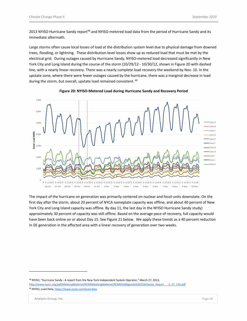
Climate Change Phase II September 2020
Analysis Group, Inc. Page 46
2013 NYISO Hurricane Sandy report48 and NYISO‐metered load data from the period of Hurricane Sandy and its
immediate aftermath.
Large storms often cause local losses of load at the distribution system level due to physical damage from downed
trees, flooding, or lightning. These distribution‐level losses show up as reduced load that must be met by the
electrical grid. During outages caused by Hurricane Sandy, NYISO‐metered load decreased significantly in New
York City and Long Island during the course of the storm (10/29/12 ‐ 10/30/12, shown in Figure 20 with dashed
line, with a nearly linear recovery. There was a nearly complete load recovery the weekend by Nov. 10. In the
upstate zone, where there were fewer outages caused by the hurricane, there was a marginal decrease in load
during the storm, but overall, upstate load remained consistent. 49
Figure 20: NYISO‐Metered Load during Hurricane Sandy and Recovery Period
The impact of the hurricane on generation was primarily centered on nuclear and fossil units downstate. On the
first day after the storm, about 20 percent of NYCA nameplate capacity was offline, and about 40 percent of New
York City and Long Island capacity was offline. By day 11, the last day in the NYISO Hurricane Sandy study)
approximately 30 percent of capacity was still offline. Based on the average pace of recovery, full capacity would
have been back online on or about Day 15. See Figure 21 below. We apply these trends as a 40 percent reduction
in DE generation in the affected area with a linear recovery of generation over two weeks.
48 NYISO, “Hurricane Sandy ‐ A report from the New York Independent System Operator,” March 27, 2013,
http://www.nysrc.org/pdf/MeetingMaterial/RCMSMeetingMaterial/RCMS%20Agenda%20159/Sandy_Report___3_27_133.pdf 49 NYISO, Load Data, https://www.nyiso.com/load‐data
0
1,000
2,000
3,000
4,000
5,000
6,000
7,000
0 6 1218 0 6 1218 0 6 1218 0 6 1218 0 6 1218 0 6 1218 0 6 1218 0 6 1218 0 6 1218 0 6 1218 0 6 1218 0 6 1218 0 6 1218 0 6 1218 0 6 1218 0 6 1218
26‐Oct 27‐Oct 28‐Oct 29‐Oct 30‐Oct 31‐Oct 1‐Nov 2‐Nov 3‐Nov 4‐Nov 5‐Nov 6‐Nov 7‐Nov 8‐Nov 9‐Nov 10‐Nov
Zonal Load
(MW)
Zone A
Zone B
Zone C
Zone D
Zone E
Zone F
Zone G
Zone H
Zone I
Zone J
Zone K

Climate Change Phase II September 2020
Analysis Group, Inc. Page 47
Figure 21: Cumulative Generating Capacity Recovery during Hurricane Sandy Recovery Period
The transmission impact was severe downstate and affected both interstate and intrastate transmission lines.
According to the NYISO report: “Essentially, the seven southernmost interconnections to southeastern New York
were disconnected, leaving Long Island and New York City only connected to the Eastern Interconnection via the
Lower Hudson Valley 345 kV transmission lines.” 50 By Day 11, approximately 15 percent of transmission assets
were still offline. Based on the average pace of recovery, full capacity would have been back online on or about
Day 13. See Figure 22 below. Thus, the study models transmission as being completely off line in the area affected
by the storm, with a two week linear recovery period.
Figure 22: Cumulative Transmission Recovery during Hurricane Sandy Recovery Period
There is limited evidence of effects on renewable generation, in part because there were so few installations in
Zones J and K in 2012. Sandy hit New York as a Category 1 hurricane, with max wind gusts under 100 mph during
the storm.51 Some wind generation damage would be expected given current turbine storm ratings, but future
installations may be hardened to withstand Sandy‐level wind speeds.52 Solar panels are generally rated for 110‐145
50 Hurricane Sandy A report from the New York Independent System Operator,
http://www.nysrc.org/pdf/MeetingMaterial/RCMSMeetingMaterial/RCMS percent20Agenda percent20159/Sandy_Report___3_27_133.pdf 51 National Weather Service, “Hurricane Sandy,” https://www.weather.gov/okx/HurricaneSandy 52 General Electric, “Riders On The Storm: GE Is Building A Wind Turbine That Can Weather Violent Typhoons, Hurricanes,” June 17, 2018,
https://www.ge.com/news/reports/riders‐storm‐ge‐building‐wind‐turbine‐can‐weather‐violent‐typhoons‐

Climate Change Phase II September 2020
Analysis Group, Inc. Page 48
mph winds, and damage to both rooftop solar and grid‐connected solar during Hurricane Sandy was limited.53
Based on this information, wind generation is modeled as being off during the storm and then as having a two
week linear recovery period for repairs. Solar generation is modeled at a 50 percent reduction due to cloud cover
impacts during Day 1 of the storm, with a full next‐day recovery after the storm ends.
The most recent historical experience is from Hurricane Sandy, but future storms may not necessarily be
geographically centered on downstate zones. As a result, the study models upstate and offshore storm scenarios
using the same level of impact as the downstate scenario, but with shifts in the geographic center of storm
damage. For the upstate storm scenarios, the analysis models the same magnitude of effects, but focused on
Zones A‐F instead of G‐K. For the offshore storm scenario, we similarly apply the same magnitude of effects, but
only to impact offshore wind generation in Zones J and K.
As a result of the findings described above, the model setup for Hurricane/Coastal wind storm scenario is
calibrated using the Hurricane Sandy data, as follows:
Load: 30 percent reduction in load in Zones G‐K; 11 day linear recovery period.
Transmission: cut off transmission lines to downstate Zones G‐K; 14 day linear recovery period.
Generation:
o Wind Generation ‐ Off in Zones J‐K during one‐day storm; 14 day linear recovery period.
o Solar Generation ‐ 50 percent decrease in Zones G‐K during one day storm; next day recovery.
o DE Generation ‐ 40 percent decrease in Zones G‐K; 14 day linear recovery period.
Severe Wind Storm – Upstate is calibrated using the downstate Hurricane Sandy effects:
Load: 30 percent reduction in load in Zones A‐F; 11 day linear recovery period.
Transmission: cut off transmission lines to upstate Zones A‐F; 14 day linear recovery period.
Generation:
o Wind Generation ‐ Off in Zones A‐F during 1‐day storm; 14 day linear recovery period.
o Solar Generation ‐ 50 percent Decrease in Zones A‐F during one day storm; next day recovery.
o DE Generation ‐ 40 percent Decrease in Zones A‐F; 14 day linear recovery period.
Severe Wind Storm ‐ Offshore
Wind Generation ‐ Off in Zones J‐K during one‐day storm; 14 day linear recovery period.
hurricanes?utm_source=feedburner&utm_medium=feed&utm_campaign=Feed percent3A percent20gereports percent2Ffeed percent20 percent28GE
percent20Reports percent29#:~:text=wind percent20energy‐,Riders percent20On percent20The percent20Storm percent3A percent20GE percent20Is
percent20Building percent20A percent20Wind percent20Turbine,Can percent20Weather percent20Violent percent20Typhoons percent2C
percent20Hurricanes&text=So percent20GE percent20Renewable percent20Energy percent20is,per percent20second percent2C percent20or
percent20128 percent20mph 53 IEEE Spectrum, “Rooftop Solar Stood Up to Sandy,” November 16, 2012, https://spectrum.ieee.org/green‐tech/solar/rooftop‐solar‐stood‐up‐to‐sandy
and Christian Science Monitor, “Are renewables stormproof? Hurricane Sandy tests solar, wind,” November 19, 2012,
https://www.csmonitor.com/Environment/Energy‐Voices/2012/1119/Are‐renewables‐stormproof‐Hurricane‐Sandy‐tests‐solar‐wind

Climate Change Phase II September 2020
Analysis Group, Inc. Page 49
4. Other Climate Impacts
In addition to the disruptions discussed above, we modeled two season‐specific climate impacts: summer droughts
and winter icing events.
A potential impact of climate change and rising average temperatures is the increased probability of a drought in
New York, which would affect hydroelectric production during summer months. According to the NYSERDA
ClimAID report, “[s]hort‐duration warm season droughts will more likely than not become more common.”54
Based on NYISO operations information on historical low water periods, we assume a 50 percent reduction in
hydroelectric production during the entire 30 day modeling period in the drought disruption.
Summer drought
Hydroelectric Generation ‐ 50 percent of baseline production across all of New York State
Finally, NYISO historical experience with severe winter conditions has shown the potential for short‐term icing
events that would damage upstate transmission lines and would reduce wind production. Historical evidence is
not fully available for the effect of icing in upstate New York on wind production, but one engineering study has
shown the potential for up to 50 percent reduction in wind production at wind farms due to ice accretion on
turbine blades.55
Icing Event (Winter only)
Load: 25 percent reduction in load in Zones A‐C; seven day linear recovery period.
Transmission: cut off transmission lines to upstate Zones A‐C; seven day linear recovery period.
Wind Generation ‐ 50 percent reduction in Zones A‐C during one‐day event; seven day linear recovery
period.
Construction of Combination Cases
Finally, to test the joint impact of differences in season, load scenarios, resource sets, and short‐term physical
disruptions, combination “cases” of each were modeled. All combination cases are presented in Table 15. The
results from these cases are presented in Section VI.
54 NYSERDA ClimAID, p.16 55 Iowa State University News Service, “Engineers study icing/de‐icing of wind turbine blades to improve winter power production,” September 23, 2019.

Climate Change Phase II September 2020
Analysis Group, Inc. Page 50
Table 15: List of Modeled Combination Cases
Climate Change Phase II Resource Set Grid in Transition Resource Set
CLCPA Reference CLCPA Reference
ID Event Summer Winter Shoulder Summer Winter Shoulder Summer Winter Summer Winter
Baseline None X X X X X X X X X X
A Heat Wave X X X
B Cold Wave X X X
C Wind Lull - Upstate X X X X X X
D Wind Lull - Off-Shore X X X X X X
E Wind Lull - State-Wide X X X X X X
F Hurricane/Coastal Wind Storm X X X
G Severe Wind Storm – Upstate X X X X X X
H Severe Wind Storm – Offshore X X X X X X X
I Drought X X X
J Icing Event X X X

Climate Change Phase II September 2020
Analysis Group, Inc. Page 51
V. Output Metrics
Model Output
The energy balance model is run for each case identified for analysis. As described in Section IV, each case is a
combination of a load scenario, resource set, and physical disruption. The model proceeds through an electricity
transfer and dispatch sequence based on the data inputs described above, including physical constraints on unit
operations and the flow of power between locations within New York. Results are presented along several metrics
indicating system reliability performance, including the identification of potential loss of load occurrences. The
results are assessed both individually for each case, and across all combination cases. This section describes the
model output metrics and graphics, followed by the process used to distill case results into a set of key
observations.
For each model run, the energy balance model estimates or tracks:
a. Hourly demand for electricity;
b. Hourly generation from renewable resources;
c. Hourly dispatch and stored energy for battery and pumped storage units;
d. Total hourly zonal generation relative to electrical demand;
e. Hourly capacity imports and transfers of power between Zones;
f. Hourly activation of price‐responsive demand resources, when needed to avoid loss of load;
g. Hourly dispatch of DE resources, when needed to avoid loss of load;
h. Magnitude of potential loss of load on an hourly basis, in each zone, over the thirty‐day modeling
period.
The central focus of the model outputs are the magnitudes, duration and frequency of use of DE resources, and
potential loss of load occurrences. In order to assist in the detailed analysis of each case, and for comparison of
potential LOLO drivers across cases, the model generates a consistent set of tables and graphics for each case. For
illustration of the reporting outputs on case outcomes, Figure 23 through Figure 28Error! Reference source not
found. present an example of the full set of metrics generated in graphical and tabular form for one case ‐ namely
the case run with the most observed loss of load occurrences (CLCPA Winter Severe Wind Storm ‐ Upstate).

Climate Change Phase II September 2020
Analysis Group, Inc. Page 52
Figure 23: Example of Hourly Results Summary
Hourly Results SummaryCase Name: CLCPA Case ‐ Winter ‐ Climate Change Phase II Resource Set ‐ Severe Wind Storm ‐ Upstate
Realistic Case w/ High Renewables (HR)
Load
Total Hrs. 720
Total MWh 26,633,154
Avg. MW 36,990.5
PRD Deployment
Total Hrs. 325
Total MWh 623,946
Avg. MW 1,919.8
Battery Deployment
Total Hrs. 262
Total MWh 856,262
Avg. MW 3,268.2
DE Resource Deployment
Total Hrs. 369
Total MWh 3,822,059
Avg. MW 10,357.9
Loss of Load Occurrences
Total Hrs. 45
Total MWh 22,150
Avg. MW 492.2
0
20,000
40,000
60,000
0 24 48 72 96 120 144 168 192 216 240 264 288 312 336 360 384 408 432 456 480 504 528 552 576 600 624 648 672 696
MW
Load During Modeling Period
0
1,500
3,000
4,500
6,000
0 24 48 72 96 120 144 168 192 216 240 264 288 312 336 360 384 408 432 456 480 504 528 552 576 600 624 648 672 696
MW
Price Responsive Demand Deployed During Modeling Period
0
4,000
8,000
12,000
16,000
0 24 48 72 96 120 144 168 192 216 240 264 288 312 336 360 384 408 432 456 480 504 528 552 576 600 624 648 672 696
MW
Battery Energy Storage Deployed During Modeling Period
0
10,000
20,000
30,000
40,000
0 24 48 72 96 120 144 168 192 216 240 264 288 312 336 360 384 408 432 456 480 504 528 552 576 600 624 648 672 696
MW
DE Resource Deployed During Modeling Period
0
1,000
2,000
3,000
4,000
0 24 48 72 96 120 144 168 192 216 240 264 288 312 336 360 384 408 432 456 480 504 528 552 576 600 624 648 672 696
MW
Loss of Load Occurrences During Modeling Period
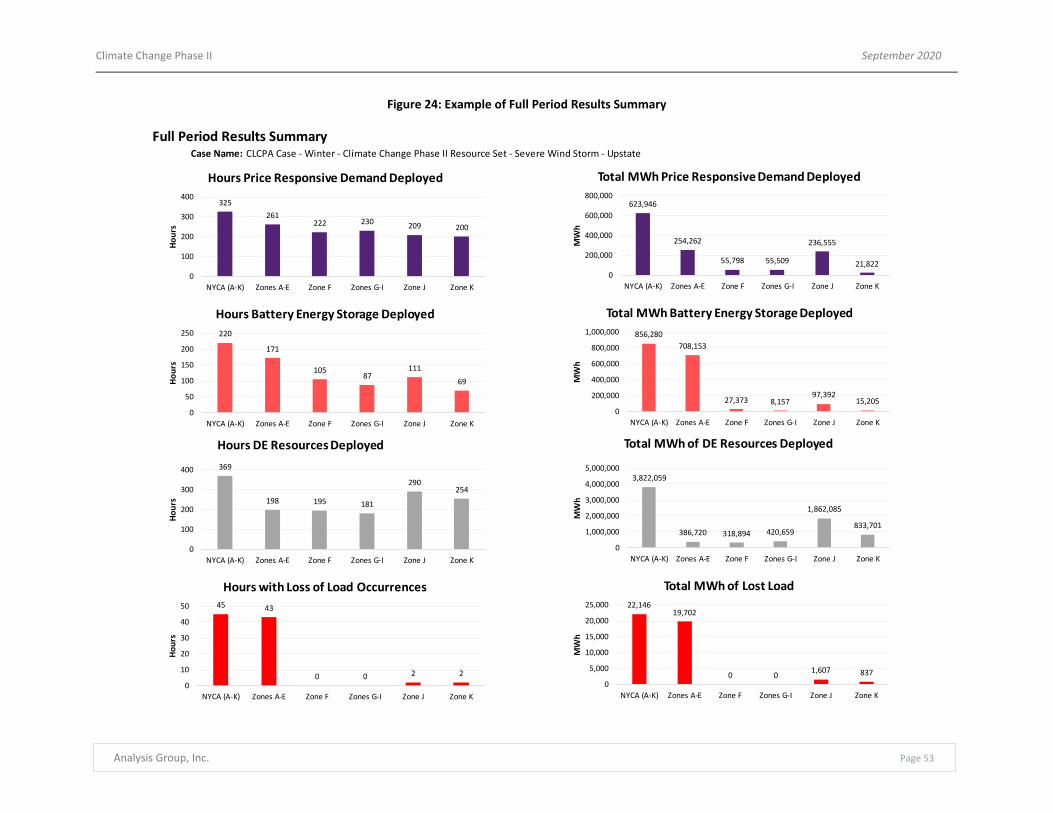
Climate Change Phase II September 2020
Analysis Group, Inc. Page 53
Figure 24: Example of Full Period Results Summary
Full Period Results SummaryCase Name: CLCPA Case ‐ Winter ‐ Climate Change Phase II Resource Set ‐ Severe Wind Storm ‐ Upstate
325
261222 230 209 200
0
100
200
300
400
NYCA (A‐K) Zones A‐E Zone F Zones G‐I Zone J Zone K
Hours
Hours Price Responsive Demand Deployed
623,946
254,262
55,798 55,509
236,555
21,822
0
200,000
400,000
600,000
800,000
NYCA (A‐K) Zones A‐E Zone F Zones G‐I Zone J Zone K
MWh
Total MWh Price Responsive Demand Deployed
45 43
0 0 2 2
0
10
20
30
40
50
NYCA (A‐K) Zones A‐E Zone F Zones G‐I Zone J Zone K
Hours
Hours with Loss of Load Occurrences22,146
19,702
0 01,607 837
0
5,000
10,000
15,000
20,000
25,000
NYCA (A‐K) Zones A‐E Zone F Zones G‐I Zone J Zone K
MWh
Total MWh of Lost Load
369
198 195 181
290254
0
100
200
300
400
NYCA (A‐K) Zones A‐E Zone F Zones G‐I Zone J Zone K
Hours
Hours DE Resources Deployed
3,822,059
386,720 318,894 420,659
1,862,085
833,701
0
1,000,000
2,000,000
3,000,000
4,000,000
5,000,000
NYCA (A‐K) Zones A‐E Zone F Zones G‐I Zone J Zone K
MWh
Total MWh of DE Resources Deployed
220
171
10587
111
69
0
50
100
150
200
250
NYCA (A‐K) Zones A‐E Zone F Zones G‐I Zone J Zone K
Hours
Hours Battery Energy Storage Deployed
856,280
708,153
27,373 8,15797,392
15,2050
200,000
400,000
600,000
800,000
1,000,000
NYCA (A‐K) Zones A‐E Zone F Zones G‐I Zone J Zone K
MWh
Total MWh Battery Energy Storage Deployed

Climate Change Phase II September 2020
Analysis Group, Inc. Page 54
Figure 25: Example of NYCA Hourly Generation by Fuel Group
Figure 26: Example of Generation by Resource Type Over Modeling Period
0
10,000
20,000
30,000
40,000
50,000
60,000
70,000
80,000Generation and Load
(MW)
Hour
Nuclear Imports Hydro incl. Storage Offshore Wind
Land‐Based Wind Grid‐Connected Solar BTM Solar Battery Storage
Price Responsive Demand DE Resources Load + Charging Load
Aggregate Load in Period (MWh) 26,633,154
Aggregate Gen in Period (MWh) 30,709,581
Gen Surplus/Deficit (MWh) 4,076,427
Hours with Aggregate Gen Deficit 27
Hours with Load Loss in any Zone 45
Aggregate Zonal Load Loss (MWh) 22,146
26%
22%
2%8%
7%
9%
7%
0%
3%
2%
14%
Intermittent Renewables, 57%
Baseload Resources, 23%
Storage/PRD, 6%
DE Resources, 14%
Land‐based Wind
Offshore Wind
Solar (Behind‐the‐meter)
Solar (Grid Connected)
Hydro Pondage + Run‐of‐River
Nuclear
Imports
Hydro Pumped Storage
Storage
Price Responsive Demand
DE Resources
TOTAL
Total Generation MWh7,193,547
6,111,804
528,251
2,041,991
2,027,789
2,422,224
2,023,200
98,702
856,280
623,946
3,822,059
27,749,794

Climate Change Phase II September 2020
Analysis Group, Inc. Page 55
Figure 27: Example of NYCA DE Resources Generation Duration
Figure 28: Example of NYCA Loss of Load Occurrences Duration
0
5,000
10,000
15,000
20,000
25,000
30,000
35,000
40,000DE Resource Generation (MW)
Hour
Hourly Generation Generation Duration Curve
0
500
1,000
1,500
2,000
2,500
3,000
3,500
Load
Loss (MW)
Hour
Load Loss Load Loss Duration Curve

Climate Change Phase II September 2020
Analysis Group, Inc. Page 56
Analysis of Outcomes
The key focus of the analysis is on cases where there is a potential loss of load occurrence, or where leading
indicators (PRD activations and/or use of DE resources) point to tight conditions and heighted reliability risks. Each
combination case based on an initial load scenario and resource set is first reviewed and analyzed as a “baseline”
case without additional physical disruptions factors that might influence system operations. Cases are analyzed
based on usage of price responsive demand and DE resource activation, and potential load deficits. The severity of
impact, meaning the magnitude, duration, and frequency of DE resource usage or loss of load, is informative to the
properties of the DE resource needed to maintain system reliability. Aggregate energy balance patterns, peak
hour patterns, and resource ramping requirements are all reviewed. Following the “baseline” cases, the physical
disruption cases are analyzed using the same metrics to measure level of impact.
The model does not take into account other emergency actions such as voltage reduction, public appeals, or
targeted load shedding, nor does it automatically consider that there may be other steps that could be taken to
resolve any transient or minor potential outage (e.g., allowing assets to move to emergency operation ratings). In
addition, the model does not take into account the probability that the combination of scenario definition and the
physical disruptions identified in a particular case will come to fruition. The model output metrics quantify the
potential reliability consequences of each case ‐ that is, the magnitude and duration of potential LOLO (or for
leading indicators) under the modeled combinations of system scenarios and physical disruptions, but it is not
intended to replicate a probabilistic assessment of whether the conditions in question will or will not meet a
standard such as loss of load no more frequent than once in ten years.56 That type of assessment is not within the
scope of this report.
The analysis of cases is summarized in Section VI below, and Appendix C provides detailed exhibits that show
detailed diagnostic results across combination cases run.
56 NYISO is obligated to plan for a system that has the “probability (or risk) of disconnecting any firm load due to resource deficiencies, on average, not
more than once in ten years.” New York State Reliability Council, “Reliability Rules and Compliance Manual,” February 9, 2018, page. 13, available at
http://www.nysrc.org/pdf/Reliability%20Rules%20Manuals/RRC%20Manual%20V42_Final.pdf.

Climate Change Phase II September 2020
Analysis Group, Inc. Page 57
VI.Results and Observations
Overview
The purpose of this report is to evaluate whether and how a changing climate and policies to mitigate its effects
may place additional stresses on reliable power system operations in New York state. These stresses may range
from changes to load due to increasing average temperatures to more frequent and/or severe storms and other
weather events. The Phase I climate study identified the impact of increasing temperature on load. This analysis
carries that review one step further, and postulates how the changing climate depicted in the Phase I study may
affect power system operations and reliability.
Our analysis is complicated by the fact that in response to the realities and risks of climate change, New York State
is embarking, through the CLCPA, on an ambitious and challenging period of transition ‐‐ one that will require an
unprecedented level and pace of change in energy supply and use to achieve steep reductions in GHG emissions
across all sectors of the economy. The electricity sector is expected to play an outsized role in this transition ‐ both
to enable reductions in other sectors through electrification, and through a rapid decarbonization of the power
infrastructure relied on to reliably meet electricity demand. As a result, the electric system of 2040, which is the
required year for no GHG emissions from the electric sector, will look fundamentally different from the current
system. That system will need to meet growing electricity demand without any of the fossil‐fueled resources
relied upon to maintain reliability today.
Thus the context for our analysis is both an altered climate, with new and different challenges to system
operations, and a completely altered set of demand, generating, fuel and transmission resources to reliably meet
the system demand 8,760 hours each year.
In this section we review the results of our modeling of potential climate disruption scenarios in the year 2040.
We discuss the results of our model in the context of the transition to a decarbonized economy and power system
that meets the requirements of the CLCPA.
Baseline Scenario Results
1. A Note About Starting Point Resource Sets
As noted earlier, before evaluating the climate disruption scenarios we must establish a system that; (a) has
demand consistent with the Climate Change Phase I Study, (2) has a set of resources that comply with the
requirements of the CLCPA, and (3) that meets electricity demand in every hour all year.
Constructing a set of “starting point” resources is highly uncertain at this point, for a variety of reasons:
The New York power system is currently heavily dependent on natural gas fired generating units to
provide energy, to be available during high load hours, to provide critical reserves on the system, and to

Climate Change Phase II September 2020
Analysis Group, Inc. Page 58
be able to ramp up and downs on timescales of seconds, minutes, hours, and days to manage net load57
variability. At least as currently configured and fueled, these resources cannot operate in 2040;
Even retaining existing low‐carbon (nuclear, hydro) resources, there is an enormous amount of energy
and capacity needed to meet projected demand in 2040;
Currently‐available and reasonably economic resources available to make up the zonal and system‐wide
energy deficits include solar and wind resources, yet their availability is uncertain and somewhat
unpredictable. In fact, data reviewed for this report reveal that there would be long (multi‐day) “lulls” in
production from these resources. This means that almost no quantity of nameplate capacity from these
resources is sufficient to meet demand in all hours of the year;
Energy storage resources that are currently and expected to be available can fill part, but not all of the
gap needed to maintain system reliability;
There is a void that will need to be filled with technologies and/or fuels that ‐ at the scales that would be
required ‐ are currently neither proven nor economic; and
There is no doubt a major amount of technological change that will happen over the next twenty years,
rendering it very difficult to forecast a future resource set with reasonable confidence.
Thus constructing a “starting point” resource set on which to model system reliability in 2040 is highly subjective.
There are innumerable potential combinations of generating resources (current and future), storage resources,
transmission expansions, distributed resources, and demand management practices that could evolve to meet
future demand. Therefore, we construct a starting point recess with a few core principles in mind:
(1) The state of New York has embarked on an aggressive path to facilitate the rapid development and siting of
zero‐carbon renewable energy resources to ensure reasonable progress towards the ultimate CLCPA requirements.
Based on this, we focus as a first step on constructing a resource set that relies on the build out of solar and wind
resources in all zones.
(2) The potential for development of substantial renewable resources exists somewhat distant ‐ upstate and
offshore ‐ from the downstate region where load is concentrated in the state. Thus, relying on renewable
resources to facilitate the transition of energy supply and demand in New York will require substantial increases in
inter‐zonal transfer capability through the development and construction of new high‐voltage transmission
capacity.
(3) Based on current technologies and the Phase I study assumptions about the shape of electricity demand in
2040, there could be periods of time when all of the retained resources and renewable generating output are not
sufficient on their own to meet demand. While we cannot know what or which technologies may emerge to fill
any gaps, we do include the DE resource to identify the nature and magnitude of residual need.
One point is worth repeating ‐ this is but one approach to constructing a starting point resource set. The GIT
resource set ‐ which we also evaluate in the model ‐ may be viewed as a bookend approach to the CCP2 resource
set. The GIT resource set does not have increases to the transmission system and therefore results in a smaller set
of renewable generation which is located closer to the downstate load and also results in relying more on the DE
resource. Thus while there are many other ways in which the grid will evolve in the coming decades, the two
resource sets we evaluate in this study may be viewed to some extent as bookends on potential outcomes.
57 “Net load” is used to represent the varying second‐by‐second level of demand on the bulk power system, net of the impact of energy efficiency,
demand response, and behind‐the‐meter generating resources (primarily solar photovoltaic).

Climate Change Phase II September 2020
Analysis Group, Inc. Page 59
Since the CCP2 resource set was designed to have sufficient capacity and transfer capability to meet peak demand
in each case (reference and CLCPA), it is worth reviewing results of running the system for all hours in the modeling
periods with this resource set in place. Primarily, this gives us a view into how much and how often the system
requires the operation of the DE resource, but it also demonstrates quantitatively the challenges of reliable system
operations with a system configured with existing zero‐carbon resource and storage technologies.
While from an annual energy standpoint the DE resources provide only minor contributions, in both the summer
and winter modeling periods, the DE resources are critical to maintaining system reliability during hours when the
system is stressed, either from high loads, low renewable capacity factors, or both. This section will summarize the
aggregate load/generation balance across the seasonal modeling periods, then discuss specific observations about
DE resource generation in various cases.
2. Aggregate Load/Generation Balance
By construction, the total amount of baseload and renewable generation in each modeling period is sufficient to
meet all load in that period if there were no deliverability or storage constraints. For example, in the CLCPA winter
load scenario (as shown in Figure 30), in the peak load month, aggregate baseload and renewable generation is
28,493 GWh, more than the total load of 27,322 GWh. However, due to the existence of limits on inter‐zonal
transfer capability in certain hours (even with some expansion of the transmission system) and finite storage
quantities, the realized resource mix used to meet load includes 12 percent DE resources and price responsive
demand, meaning that renewables, either in terms of concurrent generation or stored energy), are not able to be
used to provide 12 percent of load (see Figure 31).
Even assuming large increases in both transmission and storage capacity (as defined in Section III.C), sizable
variance in renewable output and load means that there will not always be enough storage capacity to meet short‐
term load/generation deficits. For example, as seen in Figure 29, in the winter CLCPA scenario, the wind capacity
factor from hours 150‐200 is 74.1 percent, which allows all storage units across the state to be charged to full
capacity (138,840 MWh) by hour 173. During hours 174‐200, an average of 18,121 MW per hour of excess
renewable capacity is effectively curtailed due to lack of storage. This period is immediately followed by the hours
of 200‐288, where the wind capacity factor is 28.5 percent and load simultaneously increases. As a result, storage
capability is completely used up by hour 226, and DE resource generation is needed to run. In other words, even
though there is enough renewable generation to meet loads in winter, due to its intermittent nature, the energy is
not always deliverable during the times and to the locations it is needed.
The CLCPA load scenario is winter‐peaking, so the summer and shoulder modeling periods require less DE
resource generation and PRD to fulfill demand. The summer modeling period has more than enough aggregate
baseload and renewables generation of 27,760 GWh to meet load of 22,475 GWh (see Figure 32). Again, due to
transmission and storage restrictions, the analysis finds that DE resource and PRD resources are needed to provide
six percent of load (see Figure 33). The shoulder modeling period has even more surplus generation compared to
load, with aggregate baseload and renewables generation of 35,688 GWh and load of only 12,496 GWh (see Figure
34). In this modeling period, no DE resource generation is needed at all to supply load (see Figure 35).

Climate Change Phase II September 2020
Analysis Group, Inc. Page 60
Figure 29: Battery and Pumped Storage Energy Level, CCP2‐CLCPA Winter
Figure 30: Hourly Load/Generation Balance, CCP2‐CLCPA Winter
0%
10%
20%
30%
40%
50%
60%
70%
80%
90%
100%
0%
10%
20%
30%
40%
50%
60%
70%
80%
90%
100%
Renewab
le Cap
acity Factor (%
)
Energy Storage
Leve
l (% of Max)
Hour
Hourly Energy Level Renewable Generation
0
10,000
20,000
30,000
40,000
50,000
60,000
70,000
80,000
Generation and Load
(MW)
Hour
Nuclear Imports Hydro incl. Storage Offshore Wind
Land‐Based Wind Grid‐Connected Solar BTM Solar Battery Storage
Price Responsive Demand DE Resources Load + Charging Load
Aggregate Load in Period (MWh) 27,322,037
Aggregate Gen in Period (MWh) 32,894,710
Gen Surplus/Deficit (MWh) 5,572,673
Hours with Aggregate Gen Deficit 0
Hours with Load Loss in any Zone 0
Aggregate Zonal Load Loss (MWh) 0

Climate Change Phase II September 2020
Analysis Group, Inc. Page 61
Figure 31: Generation by Resource Type, CCP2‐CLCPA Winter
Figure 32: Hourly Load/Generation Balance, CCP2‐CLCPA Summer
33%
20%2%
7%
7%
9%
7%
0%
3%
2%
10%
Renewables, 62%
Baseload Resources, 23%
Storage/PRD, 5%
DE Resources, 10%
Land‐based Wind
Offshore Wind
Solar (Behind‐the‐meter)
Solar (Grid Connected)
Hydro Pondage + Run‐of‐River
Nuclear
Imports
Hydro Pumped Storage
Storage
Price Responsive Demand
DE Resources
TOTAL
Total Generation MWh9,374,434
5,802,535
502,770
1,947,522
2,027,789
2,422,224
2,023,200
104,056
878,087
544,857
2,866,203
28,493,677
0
10,000
20,000
30,000
40,000
50,000
60,000
70,000
80,000
Generation and Load
(MW)
Hour
Nuclear Imports Hydro incl. Storage Offshore Wind
Land‐Based Wind Grid‐Connected Solar BTM Solar Battery Storage
Price Responsive Demand DE Resources Load + Charging Load
Aggregate Load in Period (MWh) 22,475,955
Aggregate Gen in Period (MWh) 27,760,491
Gen Surplus/Deficit (MWh) 5,284,536
Hours with Aggregate Gen Deficit 0
Hours with Load Loss in any Zone 0
Aggregate Zonal Load Loss (MWh) 0
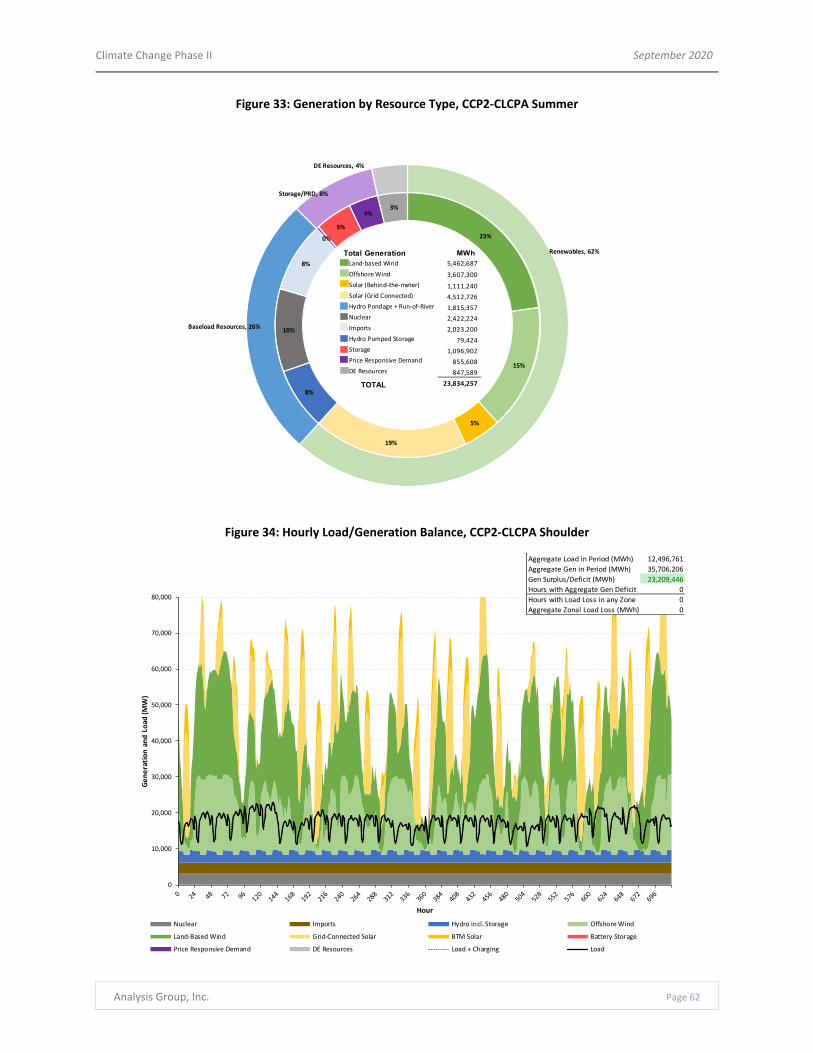
Climate Change Phase II September 2020
Analysis Group, Inc. Page 62
Figure 33: Generation by Resource Type, CCP2‐CLCPA Summer
Figure 34: Hourly Load/Generation Balance, CCP2‐CLCPA Shoulder
23%
15%
5%
19%
8%
10%
8%
0%
5%
4%3%
Renewables, 62%
Baseload Resources, 26%
Storage/PRD, 8%
DE Resources, 4%
Land‐based Wind
Offshore Wind
Solar (Behind‐the‐meter)
Solar (Grid Connected)
Hydro Pondage + Run‐of‐River
Nuclear
Imports
Hydro Pumped Storage
Storage
Price Responsive Demand
DE Resources
TOTAL
Total Generation MWh5,462,687
3,607,300
1,111,240
4,512,726
1,815,357
2,422,224
2,023,200
79,424
1,096,902
855,608
847,589
23,834,257
0
10,000
20,000
30,000
40,000
50,000
60,000
70,000
80,000
Generation and Load
(MW)
Hour
Nuclear Imports Hydro incl. Storage Offshore Wind
Land‐Based Wind Grid‐Connected Solar BTM Solar Battery Storage
Price Responsive Demand DE Resources Load + Charging Load
Aggregate Load in Period (MWh) 12,496,761
Aggregate Gen in Period (MWh) 35,706,206
Gen Surplus/Deficit (MWh) 23,209,446
Hours with Aggregate Gen Deficit 0
Hours with Load Loss in any Zone 0
Aggregate Zonal Load Loss (MWh) 0

Climate Change Phase II September 2020
Analysis Group, Inc. Page 63
Figure 35: Generation by Resource Type, CCP2‐CLCPA Shoulder
3. Peak Hour Patterns
DE resources have a particular role to play during the peak load hours of each modeling period. Figure 36 shows
that during the peak hour in the winter CLCPA scenario (hour 2 of January 12, 2040), DE resources provide 59
percent of demand. It happens that in the winter peak hour, solar generators on aggregate have a 0 percent
capacity factor, and wind generators have on aggregate a 17 percent capacity factor. As a result, DE resources
provide the majority of energy on the peak winter hour.
By contrast, Figure 36 shows that during the peak load hour during the summer CLCPA scenario (Hour 17 of July
18, 2040), the entirety of load is met by the ample amount of renewable resources, baseload resources, storage,
and PRD, and no DE resource generation is required. In the summer peak hour, solar generators on aggregate
have a 24.0 percent capacity factor, and wind generators have on aggregate a 24.2 percent capacity factor, enough
to meet load needs. However, there are several hours in the summer that, due to reduced renewable output, that
significant amounts of DE resources are required to serve load. Additionally, even though the results from this
analysis did not show the need for DE resources during the spring load levels, there is always the potential, given
the nature of renewable resources, for the need for DE resources.
21%
15%
2%
9%17%
20%
16%
0%0%0%0%
Renewables, 47%
Baseload Resources, 53%
Storage/PRD, 0%
DE Resources, 0%
Land‐based Wind
Offshore Wind
Solar (Behind‐the‐meter)
Solar (Grid Connected)
Hydro Pondage + Run‐of‐River
Nuclear
Imports
Hydro Pumped Storage
Storage
Price Responsive Demand
Generic Dispatchable
TOTAL
Total Generation MWh2,661,916
1,799,474
289,509
1,162,669
2,125,506
2,422,224
2,023,200
‐
4,852
13,119
‐
12,502,468

Climate Change Phase II September 2020
Analysis Group, Inc. Page 64
Figure 36: Resource Mix during Seasonal Peak Load Hours (CCP2‐CLCPA Case)
4. Ramping Patterns
Another important requirement for the DE resource is the ability to “ramp up” quickly, or increase generation over
a short period of time during the course of an operating day. Due to the large reliance on renewable generation
throughout each modeling period, there are certain hours and certain days in the modeling periods where a large
quantity of DE resource output is needed to meet load needs.
Figure 37 shows the quantity of load that is needed to be met on average by hour for each day of the Winter
CLCPA baseline case. The top black solid line shows average load over the course of the day. This load is met first
by solar and wind resources, shown by the load reductions in the dashed yellow and green lines. The final average
quantity to be met by storage, PRD, or DE resource generation is the quantity shown by the blue dashed line.
On average during the day, there is more generation than load, which means that storage capacity can be filled
from generation and DE resources are not needed to operate. Even on days when there are short lulls in resource
generation, if storage resources are filled to capacity in advance of the evening peak, storage output is sufficient to
meet load needs without dispatch of DE resources.
56%Renewables
18%Renewables
57%Renewables
20%Baseload Resources
16%Baseload Resources
43%Baseload Resources
23%Storage/PRD
7%Storage/PRD
59%DE Resources
151%, Curtailed Renewables
0
10,000
20,000
30,000
40,000
50,000
60,000
70,000
Summer Winter Shoulder
Po
we
r G
en
era
ted
in P
ea
k H
ou
r (M
W)
Load and Gen during Peak Hour:
45,643 MW
Load and Gen during Peak Hour:
52,460 MW
Gen during Peak Hour:
57,223 MW
Load during Peak Hour: 22,798 MW

Climate Change Phase II September 2020
Analysis Group, Inc. Page 65
Figure 37: Average Load and Generation Requirements, CCP2‐CLCPA Winter
Note: [1] Renewable generation quantities offset from load do not include curtailed renewable generation.
However, there is also great variance between days within the modeling period. Based on model results, there
also are short periods of less than 6 hours where output from the DE resource must be ramped from almost
nothing to almost full capacity. Figure 38 shows an example of the single day in the CLCPA Winter baseline case
where the most ramping capability is required. Between hours 14 and 20, DE resource output across the state
must increase from 362 MW (or 1.1% of DE resource nameplate capacity) to 27,434 MW (or 85.4% of nameplate
capacity). In the single hour between 15 and 16, DE resource output must increase 11,716 MW, which is the
largest single‐hour increase across the entire winter modeling period. Given the rapidity of decrease in solar
generation when the sun sets, the DE resource must have fast ramping capability in order to meet requirements
on days when other resources are not available to meet load.
‐5,000
0
5,000
10,000
15,000
20,000
25,000
30,000
35,000
40,000
45,000
Load
(MW)
Hour of the Day
Load Load Minus Solar Load Minus Solar and Wind Load Minus Renewables and Baseload (incl. Hydro, Nuclear, Imports)

Climate Change Phase II September 2020
Analysis Group, Inc. Page 66
Figure 38: Maximum Hourly Ramping Requirement, CCP2‐CLCPA Winter
Note:
[1] Renewable generation quantities offset from load do not include curtailed renewable generation.
5. Aggregate Use of Dispatchable and Emissions‐free Resources
Though DE resources provide an important function during peak hours, on average, they are rarely called upon to
supply energy. As shown in Table 16, DE resource capacity factor is only 12.4 percent in winter, 3.7 percent in
summer, and zero percent in the shoulder month for the CLCPA scenario. In addition, as shown in Figure 39, the
need for DE resources is most acute in a limited number of hours. In winter, when the system is most stressed,
over 10,000 MW of DE resources are needed for 126 hours (or 17.5 percent of the 720 hour modeling period), but
no DE resources are called upon for 465 hours (or 64.6 percent of modeled hours).
In this study, we provide results for two very different visions for the evolution of the power system ‐ one that
relies on renewables and transmission (the CCP2‐CLCPA resource set), and one that places greater emphasis on the
DE resource ‐ that is, the potential emergence of a zero‐carbon generation or fuel source (the GIT resource set). A
key difference between them is that since the GIT resource sets do include any transmission expansion, it results in
a higher degree of reliance on the DE resource. This provides insight into the challenges New York State will face in
guiding and managing what will likely be a rapid transition over the next two decades.
For example, if there is skepticism that an economic fuel or technology will emerge and be widely available, and
that can deliver reliable capacity, energy, reserves, and flexible operating attributes with little or no emissions of
‐5,000
0
5,000
10,000
15,000
20,000
25,000
30,000
35,000
40,000
Load
(MW)
Hour of the Day
Load (Average Day) Minus Renewables and Baseload (incl. Hydro, Nuclear, Imports)
Load (Max Ramp Day) Minus Renewables and Baseload (incl. Hydro, Nuclear, Imports)

Climate Change Phase II September 2020
Analysis Group, Inc. Page 67
GHGs, then the pathway may be more heavily tilted towards aggressive investment in and development of
renewable and transmission infrastructure, such as in the CCP2 resource set. This approach would allow the
system to operate with relatively low annual generation from the DE resource. Conversely, if such a fuel or
technology were to emerge, be technologically and economically viable, and be widely available, then there is little
need to invest the significant capital needed to build out renewable and transmission infrastructure to meet the
CLCPA requirements. Thus, the degree of reliance on a DE resources under different scenarios and resource sets is
evaluated in this report as an indication of the challenges New York will face to manage its energy systems
transition in the coming decades.
Table 16: DE Resource Capacity Factor by Season
Figure 39: Duration Curve of DE Resource Generation by Modeling Period
Key Observations by Physical Disruption
Season
Average Capacity
Factor
Winter 12.39%
Summer 3.66%
Shoulder 0.00%
0
5,000
10,000
15,000
20,000
25,000
30,000
35,000
40,000
DE
Re
sou
rce
Ge
ne
rati
on
(MW
)
Hour
Summer Winter Shoulder

Climate Change Phase II September 2020
Analysis Group, Inc. Page 68
1. Temperature Waves
For both the summer heat wave and winter cold wave scenarios, model results show no losses of load based on
increased reliance on DE resources, as discussed below. The combination of transmission, PRD, and DE resource
generation is sufficient to meet load in all hours. In the summer modeling period in particular, increases in solar
output partially offset declines in wind production.
In both cases, there is an increase of the use of DE resources over the baseline case. This increase is more
pronounced in the summer modeling period as compared to the winter. Based on the Phase I study temperature‐
load modeling, across all zones, higher temperatures during heat waves lead to steeper increases in load compared
to lower temperatures during cold waves. That is, a one degree increase in temperature during a summer heat
wave will lead to more additional MWs of load during the daily peak than a one degree decrease in temperature
during a winter cold wave. As a result, the summer heat wave scenario requires more DE resource generation over
the baseline scenario as compared to the winter cold wave.
Figure 40: Hourly Load/Generation Balance, CCP2‐CLCPA Summer Heat Wave Case
0
10,000
20,000
30,000
40,000
50,000
60,000
70,000
80,000
Generation and Load
(MW)
Hour
Nuclear Imports Hydro incl. Storage Offshore Wind
Land‐Based Wind Grid‐Connected Solar BTM Solar Battery Storage
Price Responsive Demand DE Resources Load + Charging Load
Aggregate Load in Period (MWh) 22,707,507
Aggregate Gen in Period (MWh) 27,902,648
Gen Surplus/Deficit (MWh) 5,195,141
Hours with Aggregate Gen Deficit 0
Hours with Load Loss in any Zone 0
Aggregate Zonal Load Loss (MWh) 0
7‐Day Heat Wave

Climate Change Phase II September 2020
Analysis Group, Inc. Page 69
Figure 41: Hourly Load/Generation Balance, CCP2‐CLCPA Winter Cold Wave Case
The heat and cold waves modeled in this study are meant to represent temperature waves that are consistent with
historical record in terms of severity and duration. More severe modeled temperature waves, as may occur more
frequently in a future with climate change, could result in increased stresses on the power system and/or greater
reliance on the DE resource.
2. Wind Lulls
According to model results, multi‐day wind lulls coincident with peak load hours can lead to significant increased
use of DE generation and loss of load. This is particularly pronounced in the most stressed month for each load
scenario, winter for the CLCPA scenario, summer for the CCP2 Reference Case.
As shown in Figure 42, a winter wind lull that overlaps with the peak load period in the CLCPA load scenario would
lead to a reliance on DE generation in order to meet demand, and 13 hours with some loss of load across all Zones.
In Figure 43, solar generation during the 12‐day summer wind lull offsets a significant portion of generation losses
from wind, with the remaining demand met by price responsive demand and an increased amount of DE resource
generation. Ultimately, there is no load loss in the summer load scenario even with the more severe wind lull than
in winter.
0
10,000
20,000
30,000
40,000
50,000
60,000
70,000
80,000
Generation and Load
(MW)
Hour
Nuclear Imports Hydro incl. Storage Offshore Wind
Land‐Based Wind Grid‐Connected Solar BTM Solar Battery Storage
Price Responsive Demand DE Resources Load + Charging Load
Aggregate Load in Period (MWh) 27,957,446
Aggregate Gen in Period (MWh) 33,528,073
Gen Surplus/Deficit (MWh) 5,570,626
Hours with Aggregate Gen Deficit 0
Hours with Load Loss in any Zone 0
Aggregate Zonal Load Loss (MWh) 0
7‐Day Cold Wave
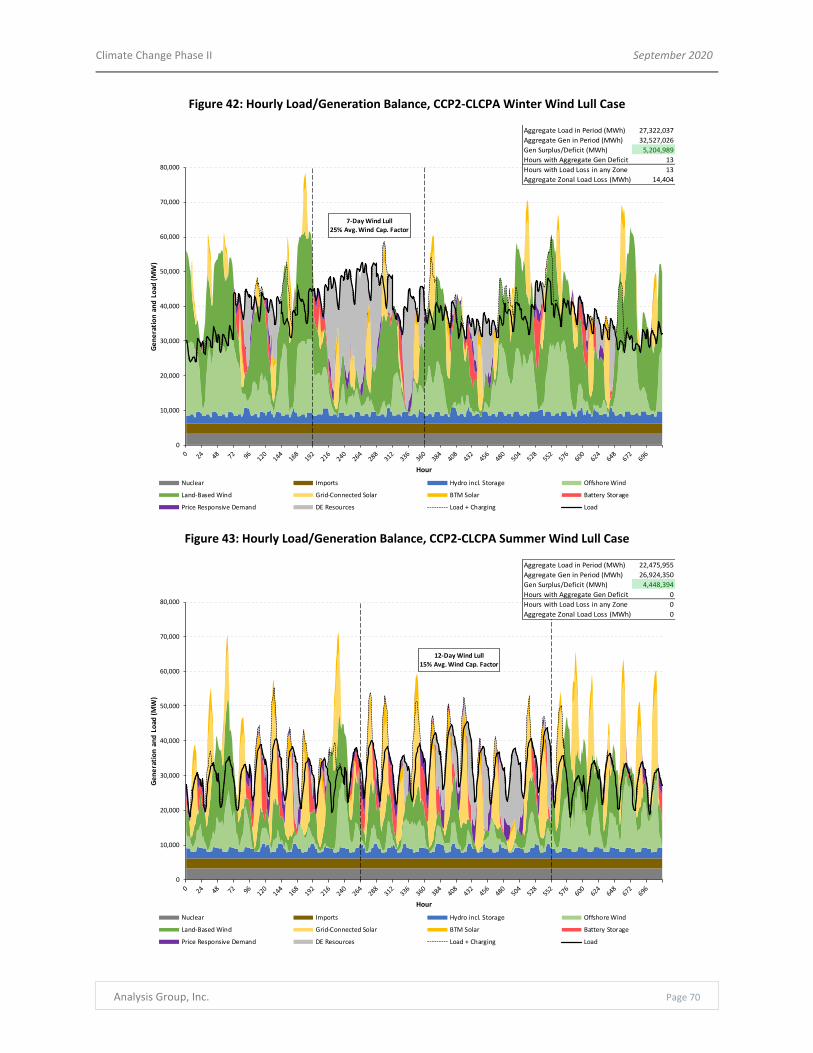
Climate Change Phase II September 2020
Analysis Group, Inc. Page 70
Figure 42: Hourly Load/Generation Balance, CCP2‐CLCPA Winter Wind Lull Case
Figure 43: Hourly Load/Generation Balance, CCP2‐CLCPA Summer Wind Lull Case
0
10,000
20,000
30,000
40,000
50,000
60,000
70,000
80,000
Generation and Load
(MW)
Hour
Nuclear Imports Hydro incl. Storage Offshore Wind
Land‐Based Wind Grid‐Connected Solar BTM Solar Battery Storage
Price Responsive Demand DE Resources Load + Charging Load
Aggregate Load in Period (MWh) 27,322,037
Aggregate Gen in Period (MWh) 32,527,026
Gen Surplus/Deficit (MWh) 5,204,989
Hours with Aggregate Gen Deficit 13
Hours with Load Loss in any Zone 13
Aggregate Zonal Load Loss (MWh) 14,404
7‐Day Wind Lull
25% Avg. Wind Cap. Factor
0
10,000
20,000
30,000
40,000
50,000
60,000
70,000
80,000
Generation and Load
(MW)
Hour
Nuclear Imports Hydro incl. Storage Offshore Wind
Land‐Based Wind Grid‐Connected Solar BTM Solar Battery Storage
Price Responsive Demand DE Resources Load + Charging Load
Aggregate Load in Period (MWh) 22,475,955
Aggregate Gen in Period (MWh) 26,924,350
Gen Surplus/Deficit (MWh) 4,448,394
Hours with Aggregate Gen Deficit 0
Hours with Load Loss in any Zone 0
Aggregate Zonal Load Loss (MWh) 0
12‐Day Wind Lull
15% Avg. Wind Cap. Factor

Climate Change Phase II September 2020
Analysis Group, Inc. Page 71
3. Storm Scenarios
The storm disruptions caused the most severe impacts to system reliability of all the cases run in the model. Based
on model results, hurricane/major wind storms can cause loss of load at the transmission system level during the
storm itself and the 14‐day recovery period, but losses ease significantly once transmission is partially restored.
Based on historical experience in Hurricane Sandy, generation, transmission, and load recover at similar paces,
which means that generators would be back online to meet increased demand when storm damage is repaired and
power is restored to end users. Quick recovery of transmission assets is vital to limiting load losses. Any loss of
transmission in downstate zones prevents batteries, renewable resources, and DE resource generation in upstate
Zones from relieving loss of load downstate.
The storm cases cause the greatest system disruption in seasons when load is highest; the winter upstate storm
case under the CLCPA load scenario shows more losses of load than the summer hurricane case. In both seasons,
the storm scenario affecting offshore wind availability shows only modest system impact ‐ there are a handful of
hours with potential for loss of load in winter and none in summer.
Figure 44: Hourly Load/Generation Balance, CCP2‐CLCPA Summer Hurricane Case
The storm scenarios were all based on historical experience with Hurricane Sandy. While the impact of that storm
was significant, the results here may understate system reliability challenges to the extent that climate change
leads to more severe or more frequent storms, especially if multiple storms occur in rapid succession.
4. Other Climate Impacts
The drought event has a limited impact on DE resource generation usage during the CLCPA scenario and no loss of
load. The lower summer loads as compared to winter means that there is enough renewable and DE resource
generation to compensate for the loss of hydroelectric capacity. The icing event leads to two hours with very small
0
10,000
20,000
30,000
40,000
50,000
60,000
70,000
80,000
Generation and Load
(MW)
Hour
Nuclear Imports Hydro incl. Storage Offshore Wind
Land‐Based Wind Grid‐Connected Solar BTM Solar Battery Storage
Price Responsive Demand DE Resources Load + Charging Load
Aggregate Load in Period (MWh) 21,600,566
Aggregate Gen in Period (MWh) 27,683,256
Gen Surplus/Deficit (MWh) 6,082,690
Hours with Aggregate Gen Deficit 1
Hours with Load Loss in any Zone 26
Aggregate Zonal Load Loss (MWh) 20,168
14‐Day Storm Recovery
Period

Climate Change Phase II September 2020
Analysis Group, Inc. Page 72
loss of load occurrences in the CLCPA winter load scenario. For the most part, other resources are able to
compensate for losses of transmission and generation during the event.
5. Case Result Summaries:
Loss of Load DE Resource Generation
Total Hours with
LOLO in at least
one Load Zone
Aggregate LOLO
(MWh)
Max Consecutive
Hours with DE
Resource Gen.
Total Hours with
DE Resource
Gen.
Aggregate DE
Resource Gen.
(MWh)
Max DE Resource
Gen. (MW)
Max 1‐hr. DE
Resource Gen.
Ramp (MW)
CLCPA Summer Scenario ‐ Climate Impact Phase II Resource Set
Baseline Summer 0 0 36 145 847,589 22,081 9,170
Heat Wave 0 0 36 147 964,668 22,081 8,642
Wind Lull ‐ Upstate 0 0 37 179 1,171,656 23,361 9,447
Wind Lull ‐ Off‐Shore 0 0 40 196 1,116,165 23,170 9,170
Wind Lull ‐ State‐Wide 0 0 40 235 1,697,161 24,440 11,605
Hurricane/Coastal Wind Storm 26 20,168 171 322 1,892,046 22,081 8,642
Severe Wind Storm – Upstate 8 1,620 87 283 2,002,682 22,081 8,642
Severe Wind Storm – Offshore 0 0 36 167 1,079,462 22,163 10,015
Drought 0 0 36 166 1,148,649 23,595 10,610
Loss of Load DE Resource Generation
Total Hours with
LOLO in at least
one Load Zone
Aggregate LOLO
(MWh)
Max Consecutive
Hours with DE
Resource Gen.
Total Hours with
DE Resource
Gen.
Aggregate DE
Resource Gen.
(MWh)
Max DE Resource
Gen. (MW)
Max 1‐hr. DE
Resource Gen.
Ramp (MW)
CLCPA Winter Scenario ‐ Climate Impact Phase II Resource Set
Baseline Winter 0 0 62 255 2,866,203 32,135 11,716
Cold Wave 0 0 62 259 2,879,947 32,135 11,716
Wind Lull ‐ Upstate 5 2,373 62 259 3,076,530 32,135 12,707
Wind Lull ‐ Off‐Shore 10 7,184 104 274 3,350,666 32,135 11,715
Wind Lull ‐ State‐Wide 13 14,404 105 278 3,653,404 32,135 12,403
Severe Wind Storm – Upstate 45 22,146 81 369 3,822,059 31,419 12,850
Severe Wind Storm – Offshore 9 4,203 103 304 3,609,785 32,135 11,715
Icing Event 2 88 62 273 2,909,437 32,135 11,716
Loss of Load DE Resource Generation
Total Hours with
LOLO in at least
one Load Zone
Aggregate LOLO
(MWh)
Max Consecutive
Hours with DE
Resource Gen.
Total Hours with
DE Resource
Gen.
Aggregate DE
Resource Gen.
(MWh)
Max DE Resource
Gen. (MW)
Max 1‐hr. DE
Resource Gen.
Ramp (MW)
Reference Summer Scenario ‐ Climate Impact Phase II Resource Set
Baseline Summer 0 0 36 183 972,444 17,059 6,520
Heat Wave 0 0 36 199 1,067,892 17,059 6,520
Wind Lull ‐ Upstate 2 729 38 209 1,175,961 17,059 5,655
Wind Lull ‐ Off‐Shore 2 1,797 41 243 1,307,211 17,059 6,380
Wind Lull ‐ State‐Wide 4 3,149 42 283 1,697,728 17,059 10,929
Hurricane/Coastal Wind Storm 76 96,295 173 349 1,637,221 17,059 6,520
Severe Wind Storm – Upstate 18 4,470 106 330 1,975,003 17,059 6,520
Severe Wind Storm – Offshore 0 0 36 241 1,249,958 17,059 7,489
Drought 11 6,383 38 209 1,305,698 17,059 5,755
Loss of Load DE Resource Generation
Total Hours with
LOLO in at least
one Load Zone
Aggregate LOLO
(MWh)
Max Consecutive
Hours with DE
Resource Gen.
Total Hours with
DE Resource
Gen.
Aggregate DE
Resource Gen.
(MWh)
Max DE Resource
Gen. (MW)
Max 1‐hr. DE
Resource Gen.
Ramp (MW)
Reference Winter Scenario ‐ Climate Impact Phase II Resource Set
Baseline Winter 0 0 4 6 9,316 3,762 2,479
Cold Wave 0 0 4 6 9,316 3,762 2,479
Wind Lull ‐ Upstate 0 0 4 6 10,646 4,213 2,400
Wind Lull ‐ Off‐Shore 0 0 9 15 48,055 6,386 3,819
Wind Lull ‐ State‐Wide 0 0 13 32 90,238 8,219 4,127
Severe Wind Storm – Upstate 10 1,146 14 56 119,192 5,809 2,283
Severe Wind Storm – Offshore 0 0 8 20 31,311 4,677 3,809
Icing Event 3 157 6 14 9,886 3,762 2,479

Climate Change Phase II September 2020
Analysis Group, Inc. Page 73
Cross‐Seasonal Effects
The resource sets evaluated in this study are designed to maintain sufficient resource availability to meet peak
seasonal demand for electricity. Thus, due to the large differences in load and renewable generation across
seasons, the modeled results show large surpluses of renewable generation during the shoulder seasons of spring
and fall. As discussed in Section III.C.2 and Table 6 earlier, wind capacity factors are highest during the shoulder
season modeling, with over 50 percent capacity factor for both land‐based and offshore wind generation. At the
same time, aggregate load is lowest in the shoulder month, with total energy demanded over the 30‐day modeling
period 54.3 percent lower than demand during the winter modeling period and 44.4 percent lower than demand
during the summer modeling period for the CLCPA load scenario (see Table 5). As a result, during the shoulder
month, there is on average 32,227 MW of “excess” potential renewable generation that is curtailed ‐ or “spilled” ‐
due to a lack of load or short‐term storage capacity (see Table 17). In fact, for each of the resource sets and load
scenarios developed for this study,58 the majority of renewable generation during the shoulder month is excess,
and is not needed to meet load or fill storage (see Table 18). The quantity of excess renewables is particularly
pronounced when looking at peak load hours. For the hour with the highest load in the shoulder season modeling
period, there is enough renewable generation to meet 208 percent of demand (see Figure 45).
Table 17: Curtailed “Excess” Renewable Generation by Seasonal Modeling Period, CLCPA Load Scenario, CCP2‐CLCPA Resource Set
Table 18: Curtailed “Excess” Shoulder Month Renewable Generation by Load Scenario and Resource Set
58 As noted, this is a key difference between the renewables/transmission‐focused resource set, and the GIT resource set. Since the GIT resource set
relies far less on renewables to meet seasonal peak loads, there is less renewable generation spilled in shoulder season months (and across the year).
Season
Aggregate Excess
Renewable
Generation (GWh)
Average Hourly
Excess Renewable
Generation (MW)
Average Hourly Percentage
of Excess Renewable
Generation (%)
Winter 4,401 6,112 13.66%
Summer 3,926 5,453 13.95%
Shoulder 23,204 32,227 75.80%
Resource Set ‐
Load Case
Aggregate Excess
Renewable
Generation (GWh)
Average Hourly Excess
Renewable Generation
(MW)
Average Percentage of
Hourly Excess of Total
Renewable Generation (%)
Climate Impact Phase II
CLCPA 23,204 32,227 75.80%
Reference 16,900 23,472 73.40%
Grid In Transition
CLCPA 17,153 23,823 64.51%
Reference 8,162 11,336 47.30%

Climate Change Phase II September 2020
Analysis Group, Inc. Page 74
Figure 45: Resource Mix during Seasonal Peak Load Hours (CLCPA Case), CCP2‐CLCPA Resource Set
Given the large quantity of excess generation during the shoulder month, there is a potential for a seasonal
storage technology to meet the energy needs of DE resource generation during the summer and winter. For
example, as seen in Table 19, the excess renewable generation in the shoulder season modeling period under the
CLCPA load scenario totaled to 23,204 GWh, and the DE resource use in the winter modeling period was just 4,401
MWh. Therefore, if a technology existed that allowed 12.4 percent of the excess renewable generation in the
shoulder month to be stored until winter ‐ e.g., through the production, processing and/or storing of renewable
natural gas or hydrogen fuel for use in generation technology ‐ then all of the winter DE resource fuel need could
be met by excess renewable energy from the shoulder season.
56%Renewables
18%Renewables
57%Renewables
20%Baseload Resources
16%Baseload Resources
43%Baseload Resources
23%Storage/PRD
7%Storage/PRD
59%DE Resources
151%, Curtailed Renewables
0
10,000
20,000
30,000
40,000
50,000
60,000
70,000
Summer Winter Shoulder
Po
we
r G
en
era
ted
in P
ea
k H
ou
r (M
W)
Load and Gen during Peak Hour:
45,643 MW
Load and Gen during Peak Hour:
52,460 MW
Gen during Peak Hour:
57,223 MW
Load during Peak Hour: 22,798 MW

Climate Change Phase II September 2020
Analysis Group, Inc. Page 75
Table 19: Shoulder Month Energy Potential as Compared to DE Resource Use, CCP2 Resource Set
Comparisons of Results with Grid in Transition Resource Set
As described in Section III.E, the Grid in Transition study resource set includes considerably more DE resource
capacity than in the resource sets developed for this study, which include more renewables and transmission. The
differences in resource mix also lead to considerable differences in results. As seen in Figure 46 and Figure 47, in
the baseline cases, the proportion of load met by DE resources in the CLCPA winter load scenario is roughly nine
percent for the AG resource set but about 20 percent for the Grid in Transition resource set. One of the main
difference between the two resource sets is the level of available transmission capacity, especially on the Total
East and Total South interfaces constraints. As shown on Table 20, those constraints are binding in a larger
percentage of hours under the Grid in Transition resource set, which means that DE resources downstate are
dispatched to produce electricity in more hours.
Shoulder Summer Winter
Dates 4/1/2040 ‐4/30/2040 7/1/2040 ‐7/30/2040 1/1/2040 ‐1/30/2040
Total DE Resource Energy Used
(GWh)0 GWh 848 GWh 2,866 GWh
Total Intermittent Renewable
Energy Curtailed (GWh)23,204 GWh 3,926 GWh 4,401 GWh
Seasonal Storage Efficiency
Needed to Meet DE Resource
Energy Need with Shoulder
Season Curtailed Energy
‐ 3.65% 12.35%
Total DE Resource Energy Used
(GWh)0 GWh 972 GWh 9 GWh
Total Intermittent Renewable
Energy Curtailed (GWh)16,900 GWh 2,660 GWh 8,467 GWh
Seasonal Storage Efficiency
Needed to Meet DE Resource
Energy Need with Shoulder
Season Curtailed Energy
‐ 5.75% 0.06%
CLCPA Case
Reference Case
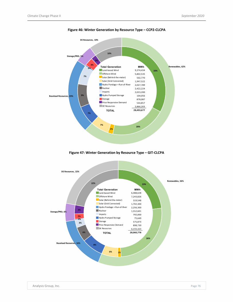
Climate Change Phase II September 2020
Analysis Group, Inc. Page 76
Figure 46: Winter Generation by Resource Type – CCP2‐CLCPA
Figure 47: Winter Generation by Resource Type – GIT‐CLCPA
33%
20%2%
7%
7%
9%
7%
0%
3%
2%
10%
Renewables, 62%
Baseload Resources, 23%
Storage/PRD, 5%
DE Resources, 10%
Land‐based Wind
Offshore Wind
Solar (Behind‐the‐meter)
Solar (Grid Connected)
Hydro Pondage + Run‐of‐River
Nuclear
Imports
Hydro Pumped Storage
Storage
Price Responsive Demand
DE Resources
TOTAL
Total Generation MWh9,374,434
5,802,535
502,770
1,947,522
2,027,789
2,422,224
2,023,200
104,056
878,087
544,857
2,866,203
28,493,677
23%
26%
1%6%
8%
6%
3%
0%2%
3%
22%Renewables, 56%
Baseload Resources, 16%
Storage/PRD, 6%
DE Resources, 22%
Land‐based Wind
Offshore Wind
Solar (Behind‐the‐meter)
Solar (Grid Connected)
Hydro Pondage + Run‐of‐River
Nuclear
Imports
Hydro Pumped Storage
Storage
Price Responsive Demand
DE Resources
TOTAL
Total Generation MWh6,488,628
7,243,826
319,548
1,702,300
2,256,300
1,552,601
792,000
75,649
575,873
898,730
6,155,323
28,060,778
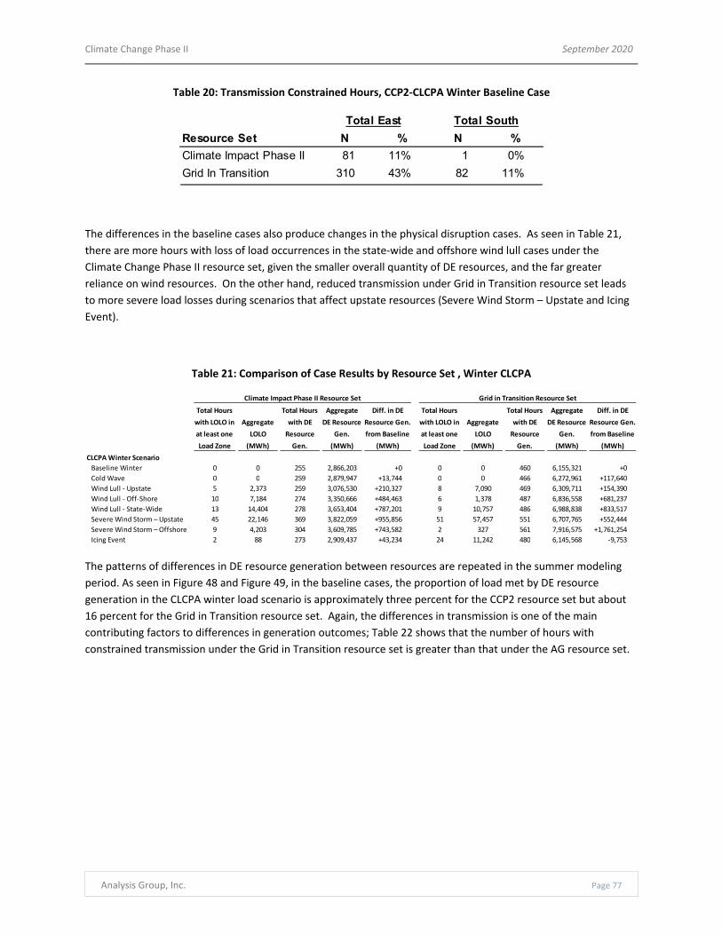
Climate Change Phase II September 2020
Analysis Group, Inc. Page 77
Table 20: Transmission Constrained Hours, CCP2‐CLCPA Winter Baseline Case
The differences in the baseline cases also produce changes in the physical disruption cases. As seen in Table 21,
there are more hours with loss of load occurrences in the state‐wide and offshore wind lull cases under the
Climate Change Phase II resource set, given the smaller overall quantity of DE resources, and the far greater
reliance on wind resources. On the other hand, reduced transmission under Grid in Transition resource set leads
to more severe load losses during scenarios that affect upstate resources (Severe Wind Storm – Upstate and Icing
Event).
Table 21: Comparison of Case Results by Resource Set , Winter CLCPA
The patterns of differences in DE resource generation between resources are repeated in the summer modeling
period. As seen in Figure 48 and Figure 49, in the baseline cases, the proportion of load met by DE resource
generation in the CLCPA winter load scenario is approximately three percent for the CCP2 resource set but about
16 percent for the Grid in Transition resource set. Again, the differences in transmission is one of the main
contributing factors to differences in generation outcomes; Table 22 shows that the number of hours with
constrained transmission under the Grid in Transition resource set is greater than that under the AG resource set.
Resource Set N % N %
Climate Impact Phase II 81 11% 1 0%
Grid In Transition 310 43% 82 11%
Total East Total South
Climate Impact Phase II Resource Set Grid in Transition Resource Set
Total Hours
with LOLO in
at least one
Load Zone
Aggregate
LOLO
(MWh)
Total Hours
with DE
Resource
Gen.
Aggregate
DE Resource
Gen.
(MWh)
Diff. in DE
Resource Gen.
from Baseline
(MWh)
Total Hours
with LOLO in
at least one
Load Zone
Aggregate
LOLO
(MWh)
Total Hours
with DE
Resource
Gen.
Aggregate
DE Resource
Gen.
(MWh)
Diff. in DE
Resource Gen.
from Baseline
(MWh)
CLCPA Winter Scenario
Baseline Winter 0 0 255 2,866,203 +0 0 0 460 6,155,321 +0
Cold Wave 0 0 259 2,879,947 +13,744 0 0 466 6,272,961 +117,640
Wind Lull ‐ Upstate 5 2,373 259 3,076,530 +210,327 8 7,090 469 6,309,711 +154,390
Wind Lull ‐ Off‐Shore 10 7,184 274 3,350,666 +484,463 6 1,378 487 6,836,558 +681,237
Wind Lull ‐ State‐Wide 13 14,404 278 3,653,404 +787,201 9 10,757 486 6,988,838 +833,517
Severe Wind Storm – Upstate 45 22,146 369 3,822,059 +955,856 51 57,457 551 6,707,765 +552,444
Severe Wind Storm – Offshore 9 4,203 304 3,609,785 +743,582 2 327 561 7,916,575 +1,761,254
Icing Event 2 88 273 2,909,437 +43,234 24 11,242 480 6,145,568 ‐9,753

Climate Change Phase II September 2020
Analysis Group, Inc. Page 78
Figure 48: Summer Generation by Resource Type ‐ CLCPA Case with CCP2 Resource Set
Figure 49: Summer Generation by Resource Type ‐ CLCPA Case with Grid in Transition Resource Set
23%
15%
5%
19%
8%
10%
8%
0%
5%
4%3%
Renewables, 62%
Baseload Resources, 26%
Storage/PRD, 8%
DE Resources, 4%
Land‐based Wind
Offshore Wind
Solar (Behind‐the‐meter)
Solar (Grid Connected)
Hydro Pondage + Run‐of‐River
Nuclear
Imports
Hydro Pumped Storage
Storage
Price Responsive Demand
DE Resources
TOTAL
Total Generation MWh5,462,687
3,607,300
1,111,240
4,512,726
1,815,357
2,422,224
2,023,200
79,424
1,096,902
855,608
847,589
23,834,257
16%
19%
3%
17%
8%
7%
3%
1%
4%
4%
18% Renewables, 55%
Baseload Resources, 18%
Storage/PRD, 9%
DE Resources, 18%
Land‐based Wind
Offshore Wind
Solar (Behind‐the‐meter)
Solar (Grid Connected)
Hydro Pondage + Run‐of‐River
Nuclear
Imports
Hydro Pumped Storage
Storage
Price Responsive Demand
DE Resources
TOTAL
Total Generation MWh3,863,788
4,596,439
693,085
3,918,407
1,983,830
1,552,601
792,000
155,854
834,108
1,030,945
4,181,951
23,603,008

Climate Change Phase II September 2020
Analysis Group, Inc. Page 79
Table 22: Transmission Constrained Hours ‐ Summer CLCPA Baseline Case
The Severe Wind Storm ‐ Upstate case also has greater losses of load under Grid in Transition resource set, due to
more limited transmission during the storm recovery period.
Table 23: Comparison of Case Results by Resource Set ‐ Summer CLCPA
Pace of Resource Change
The pace of development required to meet the capacity requirements for each resource set is historically
unprecedented in New York. As seen in Figure 50, the resource mix within New York has not changed much from
2011 through 2020. According to the NYISO Gold Books, between 2011 and 2020, the total summer capability of
grid‐connected renewable generation increased from 1,342.5 MW to 1,770.5 MW (an increase of 47.6 MW/year
on average). The only grid‐connected Solar PV power plants in New York are the Long Island Solar and Shoreham
Solar Farms, and wind generation has modestly increased from 2011 to 2020.
Resource Set N % N %
Climate Impact Phase II 12 2% 0 0%
Grid In Transition 229 32% 179 25%
Total East Total South
Climate Impact Phase II Resource Set Grid in Transition Resource Set
Total Hours
with LOLO in
at least one
Load Zone
Aggregate
LOLO
(MWh)
Total Hours
with DE
Resource
Gen.
Aggregate
DE Resource
Gen.
(MWh)
Diff. in DE
Resource Gen.
from Baseline
(MWh)
Total Hours
with LOLO in
at least one
Load Zone
Aggregate
LOLO
(MWh)
Total Hours
with DE
Resource
Gen.
Aggregate
DE Resource
Gen.
(MWh)
Diff. in DE
Resource Gen.
from Baseline
(MWh)
CLCPA Summer Scenario
Baseline Summer 0 0 145 847,589 +0 0 0 512 4,181,951 +0
Heat Wave 0 0 147 964,668 +117,079 0 0 523 4,404,209 +222,258
Wind Lull ‐ Upstate 0 0 179 1,171,656 +324,067 0 0 516 4,501,251 +319,300
Wind Lull ‐ Off‐Shore 0 0 196 1,116,165 +268,576 0 0 543 4,983,818 +801,867
Wind Lull ‐ State‐Wide 0 0 235 1,697,161 +849,572 0 0 543 5,322,997 +1,141,046
Hurricane/Coastal Wind Storm 26 20,168 322 1,892,046 +1,044,457 25 20,488 559 4,832,633 +650,682
Severe Wind Storm – Upstate 8 1,620 283 2,002,682 +1,155,093 24 18,963 549 4,998,149 +816,198
Severe Wind Storm – Offshore 0 0 167 1,079,462 +231,873 0 0 556 5,126,163 +944,212
Drought 0 0 166 1,148,649 +301,060 0 0 520 4,616,646 +434,695
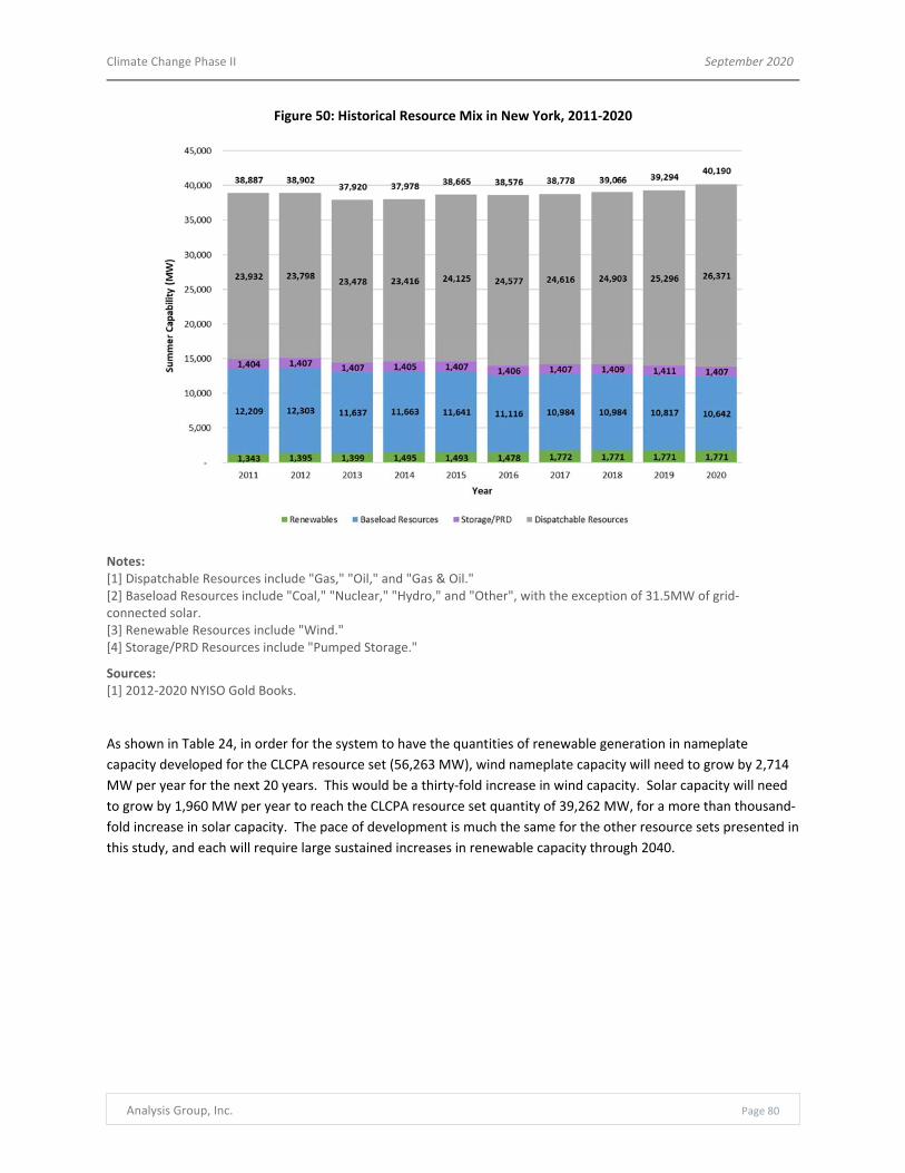
Climate Change Phase II September 2020
Analysis Group, Inc. Page 80
Figure 50: Historical Resource Mix in New York, 2011‐2020
Notes: [1] Dispatchable Resources include "Gas," "Oil," and "Gas & Oil." [2] Baseload Resources include "Coal," "Nuclear," "Hydro," and "Other", with the exception of 31.5MW of grid‐connected solar. [3] Renewable Resources include "Wind." [4] Storage/PRD Resources include "Pumped Storage."
Sources: [1] 2012‐2020 NYISO Gold Books.
As shown in Table 24, in order for the system to have the quantities of renewable generation in nameplate
capacity developed for the CLCPA resource set (56,263 MW), wind nameplate capacity will need to grow by 2,714
MW per year for the next 20 years. This would be a thirty‐fold increase in wind capacity. Solar capacity will need
to grow by 1,960 MW per year to reach the CLCPA resource set quantity of 39,262 MW, for a more than thousand‐
fold increase in solar capacity. The pace of development is much the same for the other resource sets presented in
this study, and each will require large sustained increases in renewable capacity through 2040.

Climate Change Phase II September 2020
Analysis Group, Inc. Page 81
Table 24: Required Pace of Development to Meet 2040 Resource Set Quantities
Nameplate Capacity (MW)
Required 2020‐2040 Nameplate
Capacity Growth Rate (MW/yr)
Wind (Land‐
based and
Offshore)
Grid‐Connected
Solar
Wind (Land‐
based and
Offshore)
Grid‐Connected
Solar
Existing Resources (2020) 1,985 57
Climate Phase II Reference Case
Resource Set (2040)39,962 34,354 1,899 1,715
Climate Phase II CLCPA Scenario
Resource Set (2040)56,263 39,262 2,714 1,960
Grid in Transition Reference Case
Resource Set (2040)23,522 30,043 1,077 1,499
Grid in Transition CLCPA Scenario
Resource Set (2040)48,357 31,669 2,319 1,581
Historical Nameplate Capacity Growth Rate (2012‐2020, MW/yr) 71.4 3.1

Climate Change Phase II September 2020
Analysis Group, Inc. Page 82
Observations
In this report, we have evaluated a range of climate disruption scenarios in the year 2040, and under assumptions
about the resources in place in that year. Based on our review of modeling results and the context for our analysis,
we come to the following observations:
Climate disruption scenarios involving storms and/or reductions in renewable resource output (e.g., due to wind
lulls) can lead to loss of load occurrences. Electrification, particularly in the building sector, transforms New York
into a winter‐peaking system. Thus loss of load occurrences due to climate disruptions in the winter are deeper
and occur across more scenarios than in the summer. See Table ES‐2. Specifically, in the winter severe wind
storms, lulls in wind resource output (upstate or downstate), and icing events all lead to loss of load, as well as
elevated reliance on the DE resource. In the summer, these events increase the system’s reliance on the DE
resource, but LOLOs are only triggered in the severe coastal (hurricane) and upstate wind storm events.
The variability of meteorological conditions that govern the output from wind and solar resources presents a
fundamental challenge to relying on those resources to meet electricity demand. In scenarios involving LOLOs, or
requiring substantial contributions from DE resources, periods of reduced output from wind and solar resources
are the primary driver of challenging system reliability conditions, particularly during extended wind lull events.
See Figure ES‐2, showing results for the CCP2‐CLCPA Case in the winter, including an extended wind lull. During
the wind lull,59 the state realizes losses of load in at least one zone for thirteen hours, with a total loss of over 14
gigawatt‐hours (GWh). Moreover, during the wind lull the system relies primarily on the DE generating resource to
avoid more severe LOLOs. Even outside the specific seven‐day climate disruption wind lull period, one can see that
base case reductions in wind output create periods of significant reliance on the DE resource to avoid losses of
load.60 Importantly, further increasing the nameplate capacity of such resources is of limited value, since when
output is low, it is low for all similar resources across regions or the whole state.61 As can also be seen across the full winter month, periods of solar output are not able to contribute during the early evening winter peak hours.
Battery storage resources help to fill in voids created by reduced output from renewable resources, but periods
of reduced renewable generation rapidly deplete battery storage resource capabilities. As described in Section II,
below, the CCP2‐CLCPA resource set includes the development and operation of over 15,600 MW (124.8 GWh) of
new storage resources, configured as eight‐hour batteries, and distributed throughout the state to maximize their
ability to time shift excess generation from renewable resources.62 At this level of development, battery storage
59 The wind lull is a seven‐day period from hours 192‐360 in Figure ES‐2. 60 See hours 72‐144, and hours 408‐480. 61 As noted, the generation profiles used for the wind and solar resources are taken from NREL state‐specific generation profiles, based on historical
meteorological data. The resulting renewable resource output profile across each season’s month affects both the amount of renewable capacity
needed to meet 2040 peak demand, and the reliance on the DE Resource and occurrence of LOLOs across all hours of the month. Renewable generation
technology development and/or the realization of meteorological conditions that are different than the underlying historical NREL profiles could result in
fundamentally different contributions from such resources in 2040, and different levels and types of system impacts than those reported here. The
significance of the modeled renewable generation technologies and profiles thus represents a key uncertainty in the analysis, and this should be
considered in interpreting results. 62 As noted earlier, the development of the CCP2 resource sets requires a vast buildout of carbon‐free resources to meet elevated electricity demand and
the absence of existing fossil‐fueled generating resources. This need drives the assumed amount of battery storage resources included in the resource
sets; that is, the amount of battery storage assumed reflects an assumption of continuous and significant growth in storage technology over the next
twenty years, and is well in excess of any existing mandates or near‐term development expectations.

Climate Change Phase II September 2020
Analysis Group, Inc. Page 83
makes significant contributions to avoiding loss of load and reliance on backstop generation for the immediate
period following sharp declines in renewable resource output due to climate disruptions (and also due to normal
wind/solar resource variability).63 While this represents a substantial level of assumed growth in battery storage
within New York, the contribution of storage is quickly overwhelmed by the depth of the gap left during periods of
time with a drop off in renewable generating output over periods of a day or more. This is revealed by the fill in of
the DE Resource (in grey) following depletion of the storage resources (in red) during various periods in Figure
ES‐2.
The DE resources needed to balance the system in many months must be significant in capacity, be able to come
on line quickly, and be flexible enough to meet rapid, steep ramping needs. Our generic DE resource generates
energy as needed to meet demand and avoid loss of load occurrences. This study does not make any assumptions
about what technology or fuel source can fill this role twenty years hence. Instead, the model includes the DE
Resource to identify the attributes required of whatever resource (or resources) emerges to fill this role. Based on
a review of the frequency and circumstances of reliance on the DE Resource to maintain reliability in the model,
we can identify the characteristics required of the resource. In this, certain observations stand out. First, even in
the baseline cases (i.e., before layering in climate disruption events), there are periods of very low output from the
renewable resources during periods of demand when resources need to be available to meet the bulk of the
system’s annual energy requirements. During such periods, the need for the DE Resource climbs very high ‐ at
times more than 30,000 MW. This is true even though the DE Resource is not significantly utilized on an annual
energy basis, and has a very low capacity factor, at or less than ten percent. Second, the DE Resource needs to be
highly flexible ‐ it needs to be able to come on quickly, and be able to meet rapid and sustained ramps in demand.
The results in Table ES‐2 show that the minimum one‐hour ramp requirement, even in the baseline CCP2‐CLCPA
case, approaches 12 GW, and climbs to nearly 13 GW in multiple CLCPA climate disruption cases. Moreover, as can
be seen in Figure ES‐3, the ramping capability of the DE Resource is even larger when viewed across multiple
hours. For example, the four‐hour period of greatest ramp in the CCP2‐CLCPA case in the winter exceeds 20,000
MW.
The assumed increase in inter‐zonal transfer capability in the CCP2 resource sets enables a renewables‐heavy
resource mix and improves reliability, but also increases vulnerability to certain climate disruption scenarios.
The CCP2 resource sets are designed to maximize the contribution of renewable resources which, due to available
land area and ease of siting, are heavily weighted towards the upstate region. As a result, it is necessary to assume
a major build out of the transmission system in New York, to enable the upstate renewable resources to contribute
to meeting load in the downstate region. Across the climate disruption cases, the increased transfer capability
improves the resilience of the power system to all events that are localized, such as offshore storms or wind lulls
that only affect the upstate or downstate regions, as well as to some disruptions that affect load and generation
across the state, such as heat waves and cold snaps. Conversely, the increased reliance on transmission increases
the vulnerability of the system to climate disruption events that specifically impact transmission capability,
including icing events or major storms that disable transmission capacity.
Cross‐seasonal differences in load and renewable generation could provide opportunities for renewable fuel
production. The CCP2 resource sets are constructed to be able to meet peak demand in the winter and summer
seasons based primarily on production from renewable resources. However, this means that there is a substantial
amount of renewable generation that is excess, or “spilled,” in off‐peak seasons and hours. This introduces the
potential for a seasonal storage technology to help meet the needs represented in the analysis by DE Resource
63 See, e.g., Figure ES‐3, hours 72‐96, 192‐216, and 410‐440.
Climate Change Phase II September 2020
Analysis Group, Inc. Page 84
generation during the summer and winter. Such potential assumes the emergence of economic technologies
capable of converting excess renewable energy to a fuel and storing it for later use, or the development of other
long term storage technologies. For example, as seen in Table ES‐3, the excess renewable generation in the
shoulder season modeling period under the CCP2‐CLCPA case totaled roughly 23,204 GWh, while the DE Resource
use in the winter modeling period was just 4,401 GWh. This raises the possibility that, should such technologies or
capabilities emerge, excess off‐peak renewable generation could help meet the peak‐month energy requirements
represented in the model by generation from the DE Resource.
The current system is heavily dependent on existing fossil‐fueled resources to maintain reliability, and
eliminating these resources from the mix will require an unprecedented level of investment in new and
replacement infrastructure, and/or the emergence of a zero‐carbon fuel source for thermal generating
resources. A power system that is effectively free of GHG emissions in 2040 cannot include the continued
operation of thermal units fueled by well‐based natural gas. However, these are the very units that are currently
vital to maintain power system reliability throughout the year. This is the fundamental challenge of the power
system transition that will take place over the next two decades. Indeed, this transition must take place at the
same time that electricity demand in the state will grow significantly if electrification of other economic sectors,
such as transportation and heating, is needed to meet the economy‐wide GHG emission reduction requirements.
In all four cases studied, the required investment in and development of renewable resources is substantial, and
far greater than anything previously experienced in New York. Table ES‐4 shows the pace of development required
for each case and resource set, compared to the historical capacity growth rate in New York.
Overall, the key reliability challenges identified in this study are associated with both how the resource mix
evolves between now and 2040 in compliance with the CLCPA, and the impact of climate change on
meteorological conditions and events that introduce additional reliability risks. The climate disruption events
modeled in the EBM may be more frequent and/or more severe than in the past, and this increases NYISO’s
challenges in managing reliability risks over time. Nevertheless, such events do not appear to be qualitatively
different than similar events experienced in the past, and present reliability challenges that may be considered
similar to those faced today. With sufficient planning and preparation such events could be managed to maintain
reliability in much the same way current weather‐based disruptions are managed. However, on top of this the
analysis demonstrates that, based on current information and technologies, the evolution of the system to one
focused on low/zero‐carbon resources and the infrastructure needed to support such a resource mix could
introduce a number of key vulnerabilities to system reliability. These challenges include the variability of the
meteorological conditions affecting renewable generation, the temporal limitations of existing battery storage
technologies, and the increased dependence on resources distant from load centers. Based on our analysis,
managing this transition seems to introduce reliability challenges that may be more difficult than those arising
from the conditions of a changing climate. Most importantly, this analysis suggests that establishing electricity
market designs and energy policies to encourage innovation and accelerate advanced energy resource
development will be key to reliably and economically managing the transition in the electric sector in New York.
Comparing the CCP2 resource sets to the GIT resource sets reveals key differences in how the system makeup in
2040 can affect reliability outcomes. There are key differences between the Climate Change Phase II resource sets
and those developed for the Grid in Transition study. First, given the different mixes of resources, the proportion
of load met by DE Resources in the CLCPA winter load scenario is roughly nine percent for the CCP2‐CLCPA
resource set, but about 20 percent for the GIT‐CLCPA resource set. In addition, given differences in the assumed
level of transmission on the system (the GIT resource set does not include any expansion of the current
transmission system), constraints on the Total East and Total South interfaces are binding in a larger percentage of
hours under the GIT resource set, which means that DE Resources downstate are dispatched to provide electricity

Climate Change Phase II September 2020
Analysis Group, Inc. Page 85
in more hours. The differences also lead to changes in vulnerability to climate disruptions. There are more hours
with loss of load occurrences in the state‐wide and offshore wind lull cases under the CCP2 resource sets, given the
smaller overall quantity of DE Resources and greater reliance on wind resources. Conversely, the lower level of
interzonal transfer capability in the Grid‐in‐Transition study resource set leads to more severe load losses during
scenarios that affect upstate resources, such as severe windstorm and icing events.
In this study, we provide results for two very different visions for the evolution of the power system ‐ one that
relies on renewables and transmission (the CCP2 resource sets), and one that places greater emphasis on the
backstop resource ‐ that is, the potential emergence of a zero‐carbon generation or fuel source (the GIT resource
sets). These are only two of a wide range of potential outcomes as the system and technologies change over the
next two decades, but they represent in some sense two bookends to potential system changes ‐ one focused on
aggressive system infrastructure development, and one that looks more like the current system, but is dependent
on the development of low or zero‐GHG fuel sources. The key differences between them are the relative levels of
investment in system infrastructure, and the degree of reliance on the DE Resource.
For example, if there is skepticism that an economic fuel or technology will emerge and be widely available, and
that can deliver reliable capacity, energy, reserves, and flexible operating attributes with little or no emissions of
GHGs, then the pathway may be more heavily tilted towards aggressive investment in and development of
renewable and transmission infrastructure, such as in the CCP2 resource sets. This approach would allow the
system to operate with relatively low annual generation from the DE Resource. Conversely, if such a fuel or
technology were to emerge, be technologically and economically viable, and be widely available, then there is less
need to invest the significant capital needed to build out renewable and transmission infrastructure to meet the
CLCPA requirements. These differences provide useful insight into the challenges New York State will face in
guiding and managing what will likely be a rapid transition over the next two decades.

Climate Change Phase II September 2020
Analysis Group, Inc. Page 86
VII.References
Bartos, Matthew, et. al., “Impacts of rising air temperatures on electric transmission ampacity and peak electricity
load in the United States,” Environmental Research Letters, Volume 11, 2016, available at
https://iopscience.iop.org/article/10.1088/1748‐9326/11/11/114008/pdf
The Brattle Group, “NYISO Grid in Transition Study: Detailed Assumptions and Modeling Description,” March 30,
2020, available at https://www.nyiso.com/documents/20142/11593028/2020.03.30 percent20Stakeholder
percent20Meeting percent20Deck percent20Brattle percent20FOR percent20POSTING.pdf/06562da7‐ee27‐cece‐
57f0‐afd7d688121a
The Christian Science Monitor, “Are renewables stormproof? Hurricane Sandy tests solar, wind,” November 19,
2012, available at https://www.csmonitor.com/Environment/Energy‐Voices/2012/1119/Are‐renewables‐
stormproof‐Hurricane‐Sandy‐tests‐solar‐wind
Dames and Moore, “An Assessment of Hydroelectric Pumped Storage”, November 1981, available at
https://www.iwr.usace.army.mil/Portals/70/docs/iwrreports/IWR019‐000001‐000517.pdf
EnergySage, “How hot do solar panels get? Effect of temperature on solar performance,“ Updated July 21, 2020,
available at https://news.energysage.com/solar‐panel‐temperature‐overheating/
General Electric, “Riders On The Storm: GE Is Building A Wind Turbine That Can Weather Violent Typhoons,
Hurricanes,” June 17, 2018, available at https://www.ge.com/news/reports/riders‐storm‐ge‐building‐wind‐
turbine‐can‐weather‐violent‐typhoons‐
hurricanes?utm_source=feedburner&utm_medium=feed&utm_campaign=Feed percent3A percent20gereports
percent2Ffeed percent20 percent28GE percent20Reports percent29#:~:text=wind percent20energy‐,Riders
percent20On percent20The percent20Storm percent3A percent20GE percent20Is percent20Building percent20A
percent20Wind percent20Turbine,Can percent20Weather percent20Violent percent20Typhoons percent2C
percent20Hurricanes&text=So percent20GE percent20Renewable percent20Energy percent20is,per
percent20second percent2C percent20or percent20128 percent20mph.
IEEE Spectrum, “Rooftop Solar Stood Up to Sandy,” November 16, 2012, available at
https://spectrum.ieee.org/green‐tech/solar/rooftop‐solar‐stood‐up‐to‐sandy
Iowa State University News Service, “Engineers study icing/de‐icing of wind turbine blades to improve winter
power production,” September 23, 2019, available at https://innovationia.com/2019/09/25/engineers‐study‐icing‐
de‐icing‐of‐wind‐turbine‐blades‐to‐improve‐winter‐power‐production/
Itron, “New York ISO Climate Impact Study; Phase 1: Long‐Term Load Impact,” December 2019, available at
https://www.nyiso.com/documents/20142/10773574/NYISO‐Climate‐Impact‐Study‐Phase1‐Report.pdf
National Weather Service, “Hurricane Sandy,” available at https://www.weather.gov/okx/HurricaneSandy
New York Independent System Operator, “2019 CARIS 1 70X30 Scenario Development,” September 6, 2019,
available at https://www.nyiso.com/documents/20142/8263756/07
percent20CARIS1_70x30ScenarioDevelopment.pdf/ab02dbff‐69b0‐0b2f‐04da‐8e9d0bd74b76
New York Independent System Operator, “2019 Load & Capacity Data Gold Book,” April 2019, available at
https://www.nyiso.com/documents/20142/2226333/2019‐Gold‐Book‐Final‐Public.pdf/

Climate Change Phase II September 2020
Analysis Group, Inc. Page 87
New York Independent System Operator, “Demand Response,” available at https://www.nyiso.com/demand‐
response
New York Independent System Operator, “Hurricane Sandy ‐ A report from the New York Independent System
Operator,” March 27, 2013, http://www.nysrc.org/pdf/MeetingMaterial/RCMSMeetingMaterial/RCMS
percent20Agenda percent20159/Sandy_Report___3_27_133.pdf
New York Independent System Operator, Load Data, available at https://www.nyiso.com/load‐data
New York Independent System Operator, “2019 CARIS 1 70x30 Scenario Development”, September 6, 2019,
available at https://www.nyiso.com/documents/20142/8263756/07
percent20CARIS1_70x30ScenarioDevelopment.pdf/ab02dbff‐69b0‐0b2f‐04da‐8e9d0bd74b76
NREL, “Estimating Renewable Energy Economic Potential in the United States: Methodology and Initial Results,”
August 2016, available at https://www.nrel.gov/docs/fy15osti/64503.pdf
NREL, Solar Power Database, “Solar Power Data for Integration Studies,” available at
https://www.nrel.gov/grid/solar‐power‐data.html
NREL, Wind Toolkit Database, “Wind Integration National Dataset Toolkit,” available at
https://www.nrel.gov/grid/wind‐toolkit.html
NYSERDA, “Electricity Pricing Strategies to Reduce Grid Impacts from Plug‐in Electric Vehicle Charging in New York
State”, June 2015, available at https://www.nyserda.ny.gov/‐
/media/Files/Publications/Research/Transportation/EV‐Pricing.pdf
NYSERDA, “Responding to Climate Change in New York State,” September 2014, available at
https://www.nyserda.ny.gov/‐/media/Files/Publications/Research/Environmental/ClimAID/2014‐ClimAid‐
Report.pdf
NY Senate Bill, S.6599, June 18, 2019, available at https://www.nysenate.gov/legislation/bills/2019/s6599
PJM Interconnection, “Fuel Security Analysis: A PJM Resilience Initiative,” December 17, 2018, available at
https://www.pjm.com/committees‐and‐groups/issue‐tracking/fuel‐security.aspx
Renewable Energy Magazine, “Heatwave hits European wind energy but boosts solar energy generation,” August
2018, available at https://www.renewableenergymagazine.com/wind/heatwave‐hits‐european‐wind‐energy‐but‐
boosts‐20180814
Climate Change Phase II September 2020
Analysis Group, Inc. Page 88
VIII. Glossary
C&I Commercial and industrial CARIS Congestion Assessment and Resource Integration Study CLCPA Climate Leadership and Community Protection Act EDD Effective degree day EDRP Emergency Demand Response Program EE Energy efficiency EFORd Equivalent Forced Outage Rate on Demand EIA US Energy Information Administration FERC Federal Energy Regulatory Commission GHG Greenhouse gas HQ Hydro‐Québec ICAP Installed capacity ISO Independent System Operator ISO‐NE ISO New England Inc. LI Long Island (Zone K) LOLO Loss of load occurrences MW Megawatts MWh Megawatt hour NYC New York City (Zone J) NYCA New York Control Area NYISO New York Independent System Operator, Inc. NYSERDA New York State Energy Research and Development Authority OSW Offshore wind PS Pumped storage PV Photovoltaic RTO Regional Transmission Organization SCR Special Case Resource SENY Southeastern New York (Zones G‐K) SUN Solar UPNY Upstate New York (Zones A‐F) WND Wind WT Wind turbine

Climate Change Phase II September 2020
Analysis Group, Inc. Page 89
IX.Technical Appendices
Input Data to Electric System Model
1. Phase I Load Data
The Phase 1 load data is made up of four scenarios:
Reference Case – Load growth based on Gold Book 2019 Estimates with 0.7° F per decade average
temperature increase.
Accelerated Climate Change Case – Reference Case with assumption of 1.4° F per decade average
temperature increase.
State Policy Case – Increased energy efficiency to meet NY Clean Energy Standard goals; increased BTM
PV, EV, and heating electrification.
CLCPA Case – 85 percent reduction in overall GHG by 2050, large scale electrification in residential and
commercial sectors; 85 percent reduction in transportation GHG.
This study focuses on the Reference and CLCPA cases. We further focus on three 30‐day modeling periods: Winter
(January 2040), Summer (July 2040), and Off‐peak (April 2040). The daily load for the CLCPA case winter and
summer peak days are shown below, as compared to the Reference Case winter and summer peak days.
The total load in the CLCPA winter and summer peak days is significantly higher than the Reference Case, due to
Commercial and Residential electrification loads.

Climate Change Phase II September 2020
Analysis Group, Inc. Page 90
Total demand during the shoulder, winter, and summer seasonal modeling periods is summarized below:

Climate Change Phase II September 2020
Analysis Group, Inc. Page 91
Shoulder Total Demand
Winter Total Demand
Summer Total Demand
2. NREL wind and solar profiles
Land‐based and offshore wind profiles based on 2009 synchronous NREL data. The land‐based wind data is
acquired from NREL’s Wind Toolkit Database using 721 weather sites in NY. 64 Offshore wind data is also from the
NREL Wind Toolkit Database, and uses 13 clusters of simulated offshore wind locations near NY. The simulated
data is from 2009 and aggregated at a zonal level.
Grid‐connected and BTM solar profiles based on synchronous NREL data (2006 measurements). The BTM solar
profiles uses data from NREL’s PV‐Watt tool65 for 18 stations across NY state. Grid‐connected solar date is from
NREL’s Solar Power Database66 using 62 simulated solar farm sites in NY.
All wind and solar datasets were developed by the CARIS team for the 70x30 scenario from the publicly available
simulated NREL data.
64 https://www.nrel.gov/grid/wind‐toolkit.html 65 https://pvwatts.nrel.gov/ 66 https://www.nrel.gov/grid/solar‐power‐data.html
Total Demand (GWh) Reference
Accelerated Climate Change
State Policy CLCPA
Base Load 10,304 10,388 8,509 8,509Electric Vehicles 1,081 1,081 1,342 1,342Residential Electrification 0 0 303 1,410Commercial Electrification 0 0 61 1,236
Total Adjusted Load 11,385 11,469 10,216 12,497
Total Demand (GWh) Reference
Accelerated Climate Change
State Policy CLCPA
Base Load 13,464 13,192 11,190 11,190Electric Vehicles 1,111 1,111 1,380 1,380Residential Electrification 0 0 894 7,397Commercial Electrification 0 0 673 8,129
Total Adjusted Load 14,576 14,304 14,138 28,097
Total Demand (GWh) Reference
Accelerated Climate Change
State Policy CLCPA
Base Load 18,473 19,334 15,323 15,323Electric Vehicles 1,111 1,111 1,380 1,380Residential Electrification 0 0 841 3,230Commercial Electrification 0 0 439 3,180
Total Adjusted Load 19,584 20,445 17,984 23,114

Climate Change Phase II September 2020
Analysis Group, Inc. Page 92
The below charts show the profiles for land‐based and offshore wind, and grid‐connected and BTM solar during
the peak winter and summer day of the modeling period.
‐
500
1,000
1,500
2,000
2,500
3,000
3,500
4,000
4,500
5,000Gen
eration (MW)
Day
BTM PV Generation ‐Winter
A B C D E F G H I J K
‐
500
1,000
1,500
2,000
2,500
3,000
3,500
4,000
4,500
5,000
Gen
eration (MW)
Day
BTM PV Generation ‐ Shoulder
A B C D E F G H I J K

Climate Change Phase II September 2020
Analysis Group, Inc. Page 93
‐
1,000
2,000
3,000
4,000
5,000
6,000
7,000
8,000
9,000
1/1/204
0
1/1/204
0
1/2/204
0
1/3/204
0
1/3/204
0
1/4/204
0
1/5/204
0
1/5/204
0
1/6/204
0
1/7/204
0
1/8/204
0
1/8/204
0
1/9/204
0
1/10
/204
0
1/10
/204
0
1/11
/204
0
1/12
/204
0
1/13
/204
0
1/13
/204
0
1/14
/204
0
1/15
/204
0
1/15
/204
0
1/16
/204
0
1/17
/204
0
1/18
/204
0
1/18
/204
0
1/19
/204
0
1/20
/204
0
1/20
/204
0
1/21
/204
0
1/22
/204
0
1/22
/204
0
1/23
/204
0
1/24
/204
0
1/25
/204
0
1/25
/204
0
1/26
/204
0
1/27
/204
0
1/27
/204
0
1/28
/204
0
1/29
/204
0
1/30
/204
0
1/30
/204
0
Gen
eration (MW)
Day
Land‐Based Wind Generation ‐Winter
A B C D E F G H I J K

Climate Change Phase II September 2020
Analysis Group, Inc. Page 94
3. NREL data for wind lulls
The NREL Wind Toolkit is a data set of observed wind speeds each hour from 100 meter wind turbines from 2007 –
2013.67 The power data set, used to calculate the wind profiles at three sites in New York, estimates the power
produced at each turbine site using a power curve appropriate for each site.68 The capacity factor in each hour was
then calculated by dividing the power by the maximum amount of power that the turbine can produce in one
hour.
67 https://www.nrel.gov/grid/wind‐toolkit.html
68 King, J., A. Clifton, and B.M. Hodge. 2014. Validation of Power Output for the WIND Toolkit (Technical Report, NREL/TP‐5D00‐61714). Golden, CO:
National Renewable Energy Laboratory.
‐
1,000
2,000
3,000
4,000
5,000
6,000
7,000
8,000
9,000
Gen
eration (MW)
Day
Land‐Based Wind Generation ‐ Shoulder
A B C D E F G H I J K
‐
1,000
2,000
3,000
4,000
5,000
6,000
7,000
8,000
9,000
Gen
eration (MW)
Day
Land‐Based Wind Generation ‐ Summer
A B C D E F G H I J K

Climate Change Phase II September 2020
Analysis Group, Inc. Page 114
Loss of Load Duration Curves for all Scenarios and Physical Disruptions

Climate Change Phase II September 2020
Analysis Group, Inc. Page 113
Diagnostic Charts for All Cases