Clima en España: Pasado, presente y futuroMadrid, Spain, 11 – 13 February

1 IMEDEA (UIB - CSIC), Mallorca, SPAIN.2 National Oceanography Centre, Southampton, UK.

Long-term sea level variability: what observations tell us

F. M. Calafat 1, M. Marcos 1, M. N. Tsimplis 2,

D. Gomis 1, A. Pascual1, S. Montserrat 1

• What do tide gauges tell us?

Variations of the seasonal cycle in the Mediterranean Sea and the Atlantic Iberian coast.

Mediterranean Sea level trends estimated from the longest stations.

• What does altimetry offer?

• Reconstruction of sea level fields by combining satellite altimetry and tide gauge data.

Reconstruction for the period 1993-2000.

Reconstruction for the period 1945-2000.

OVERVIEW

• Summary and conclusions

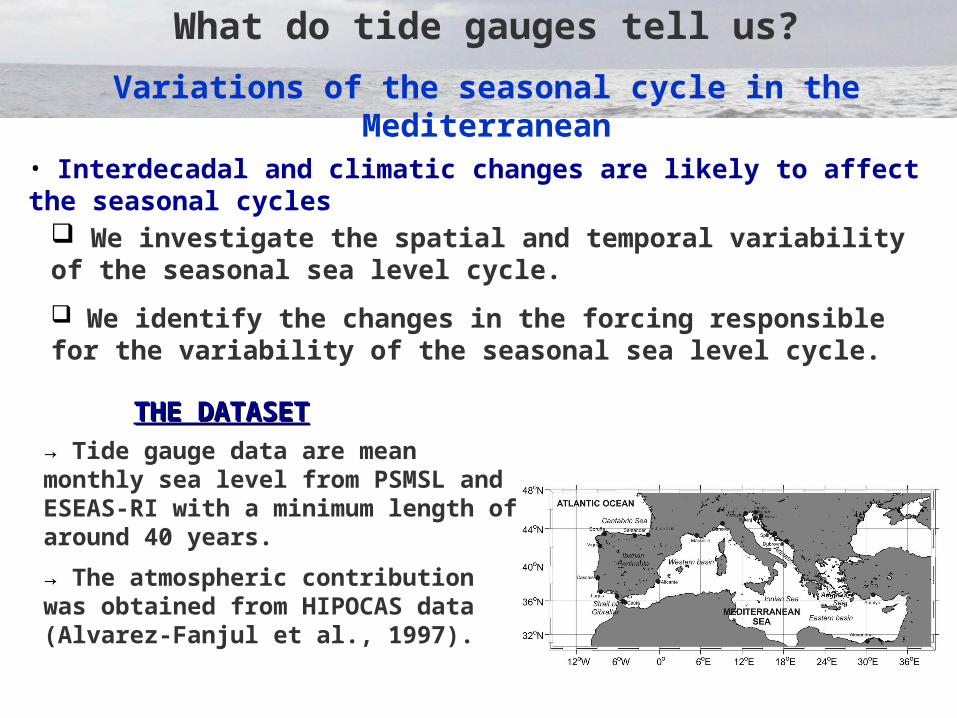
• Interdecadal and climatic changes are likely to affect the seasonal cycles

We investigate the spatial and temporal variability of the seasonal sea level cycle.

We identify the changes in the forcing responsible for the variability of the seasonal sea level cycle.

THE THE DATASETDATASET→ Tide gauge data are mean

monthly sea level from PSMSL and ESEAS-RI with a minimum length of around 40 years.

→ The atmospheric contribution was obtained from HIPOCAS data (Alvarez-Fanjul et al., 1997).

What do tide gauges tell us?

Variations of the seasonal cycle in the Mediterranean

METHODOLOGYMETHODOLOGY

The mean annual and semi-annual cycle have been estimated for each station by a least square fit of the equation:

M i Aa cos(212(t a )) Asa cos(

26(t sa ))

What do tide gauges tell us?What do tide gauges tell us?

ANNUAL SEMI-ANNUAL

Mean seasonal sea level cycle: 1962-1989Mean seasonal sea level cycle: 1962-1989

What do tide gauges tell us?What do tide gauges tell us?

What do tide gauges tell us?What do tide gauges tell us?

Temporal variability: observed sea level annual cycleTemporal variability: observed sea level annual cycle

What do tide gauges tell us?What do tide gauges tell us?

Temporal variability: Atmospherically-induced annual cycleTemporal variability: Atmospherically-induced annual cycle

→ Annual amplitude changes are very consistent in all areas, except in the eastern Mediterranean and the Cantabric stations.

→ The atmospherically-induced seasonal sea level cycle reach 4 cm . Maximum amplitudes are reached in both cases in the eastern basin.

What do tide gauges tell us?What do tide gauges tell us?

Temporal variability: residual sea level annual cycleTemporal variability: residual sea level annual cycle

→ After removing the atmospheric pressure and wind effects there is still significant temporal variability in the seasonal cycle.

→ In the Atlantic the temporal variability of the annual signal of the residuals appears more consistent between stations than that of the observations

Available data sets:

Tide gauge records: partial spatial coverage and …

they do not measure absolute sea level, but sea level relative to land marks… and land is not static

• Model corrections (GIA)

- The post glacial rebound have been corrected by means of the GIA model ICE-5G (VM2, Peltier, 2004)

Small values in the Med Sea (up to +0.3 mm/yr in the Adriatic and Aegean)

What do tide gauges tell us?

Sea level trends

→Sea level trends obtained from the 21 longest records (>35 yr) are smaller in the Mediterranean (0.3 ± 0.4 to −0.7 ± 0.3 mm/yr) than in the neighbouring Atlantic sites (1.6 ± 0.5 to –1.9 ± 0.5 mm/yr) for the period 1960–2000.

→ The atmospheric contribution accounts for 20–50 per cent of the observed yearly sea level variability and introduces negative trends of –0.2 to –0.9 mm/yr.

What do tide gauges tell us?What do tide gauges tell us?Sea level trends in Southern Europe for the period 1960-2000Sea level trends in Southern Europe for the period 1960-2000

What does altimetry offer?

MSTEP website

Altimetry data: short time coverage (from 1993)

Tide gauge dataTide gauge data

→ From the data archive of the PSMSL. All data used are Revised Local Reference data.

→ All tide gauges were corrected using the GIA values from the ICE-4G VM2 (Peltier, 2001)

→ The period of reconstruction 1945-2000 was broken into 6 smaller periods.

→ The seasonal cycle was removed from tide gauges by means of a harmonic analysis.

The satellite altimetry datasetThe satellite altimetry dataset

→ Gridded Sea Level Anomaly were collected at CLS by combining several altimeter missions.

→ The resolution of altimetry fields is 1/4º , resulting in a total of 5022 grid points covering the Mediterranean basin for the period 1993-2005.

→ The seasonal cycle was removed from altimetry data by means of a harmonic analysis.

The reconstruction of sea level fieldsF.M. Calafat and D. Gomis, 2009 in GPC

Reduced-space optimal interpolation

• We minimize for changes in sea level. That avoids the problem of locating all station in a single, constant vertical frame.

• A spatially-constant EOF (named EOF-0) is added to account for spatially uniform sea level changes.

• The method gives theoretical estimate for the error.

• Optimal interpolation accounts for non-homogeneous distributions giving less weight to highly correlated stations.

Reconstruction of Mediterranean Sea level fields for the period 1945-2000

: Spatial EOFs from altimetry data

: tide gauge data

The reconstruction of sea level fieldsThe reconstruction of sea level fields

MethodologyMethodology

Sea level trends for the period 1993-2000Sea level trends for the period 1993-2000

→ The reconstructed and observed trends are very similar, showing positive values above 10 mm/yr in the eastern Mediterranean and smaller rates in the western Mediterranean.

→ The reconstruction also reproduces the marked negative trend of more than -15 mm/yr observed in the Ionian Sea.

→ The reconstructed mean sea level rise for the period 1993-2000 is 4.0 0.7 mm/yr and 3.9 0.6 mm/yr for the altimetry .

Distribution of sea level trends for the period 1993-2000Distribution of sea level trends for the period 1993-2000

The reconstruction of sea level fieldsThe reconstruction of sea level fields

Comparison between the reconstruction and tide gauge observationsComparison between the reconstruction and tide gauge observations

→ We used tide gauge records that did not enter the computations.

→ Here we show a comparison with the tide gauge located at Alexandria.

→The correlation between the two time series is 0.7.

The reconstruction of sea level fieldsThe reconstruction of sea level fields

Distribution of sea level trends for the period 1945-2000Distribution of sea level trends for the period 1945-2000

→ Maximum positive rate in the Ionian Sea and nearly zero trends in the Aegean Sea.

→ Small positive trends in the western Mediterranean and even smaller trends in the Eastern Mediterranean.

→ Reconstruction reproduces the EMT even for the pre-altimetric period.

The reconstruction of sea level fieldsThe reconstruction of sea level fields

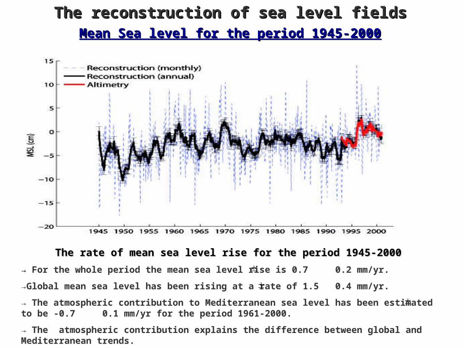
The rate of mean sea level rise for the period 1945-2000The rate of mean sea level rise for the period 1945-2000

→ For the whole period the mean sea level rise is 0.7 0.2 mm/yr.

→Global mean sea level has been rising at a rate of 1.5 0.4 mm/yr.

→ The atmospheric contribution to Mediterranean sea level has been estimated to be -0.7 0.1 mm/yr for the period 1961-2000.

→ The atmospheric contribution explains the difference between global and Mediterranean trends.

Mean Sea level for the period 1945-2000Mean Sea level for the period 1945-2000

The reconstruction of sea level fieldsThe reconstruction of sea level fields

Summary and conclusionsSummary and conclusions

• The mean seasonal sea level cycle estimated from tide-gauge records has amplitudes ranging between 3-7 cm for the annual signal and 1-3 cm for the semi-annual signal. The annual cycle reaches its maximum values mainly between September and November except in the eastern basin, where it peaks in July. The semi-annual cycle peaks mainly in January/February (in March in the eastern Mediterranean)

• The temporal evolution of the observed seasonal sea level cycle has revealed a large range of variations. During the period 1950-2000, decadal changes in annual and semi-annual signals are consistent.

• After removing the atmospheric pressure and wind effects there is still significant temporal variability in the seasonal cycle.

• The reconstruction gives, for the first time in the Mediterranean, the spatial distribution of trends spanning more than five decades.

• The distribution of sea level trends for the period 1945-2000 has as a main feature the maximum positive trend in the Ionian Sea (up to 1.2 mm/yr). Minimum values are obtained in the Aegean Sea, where trends are nearly zero.

• The rate of mean sea level rise for the period 1945-2000 is 0.7 0.2 mm/yr.

• The rate of mean sea level rise is in good agreement with global estimates if we take into account the negative trends caused by the atmospheric contribution.