Speed Studies

CIVL 4162/6162

(Traffic Engineering)

Learning Objectives

• Determine following characteristics of spot

speed

– mean, median, mode, pace, 85th percentile, sd

• Fit a speed distribution

• Check for normality

• Comparison of assumed versus observed

distribution

Introduction

• Speed data is needed for a variety of traffic

analyses

• Spot speed data refers to measurement of

individual speeds of vehicles passing a point

on a roadway.

• Care must be taken to conduct the study

appropriately so that the sample data will

adequately reflect speed characteristics of

the population.

Spot Speed Studies

• Useful for:

– Monitoring speed trends

– Establishing traffic operation and control

parameters

– Establishing highway design elements

– Evaluating highway capacity

– Assessing highway safety

– Measuring effectiveness of changes

Parameters of Interest

• Median spot speed

• Mean spot speed

• Modal spot speed

• Pace

– 10 mi/hr increment in speed in which the higher

percentage of drivers is observed

• 85th percentile speed

• Standard Deviation

Data Collection

• Individual vehicle

– Manual

– Radar

– Video

• All-vehicle sampling

– Road detectors

– Radar-based traffic sensors

– Electronic-principle detectors

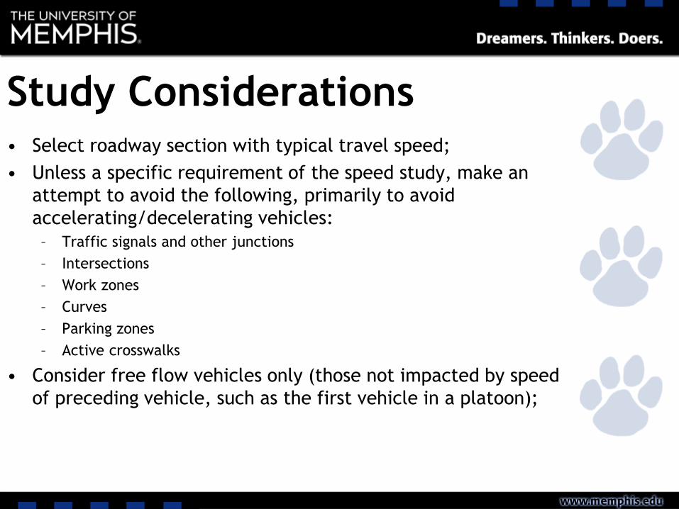
Study Considerations• Select roadway section with typical travel speed;

• Unless a specific requirement of the speed study, make an

attempt to avoid the following, primarily to avoid

accelerating/decelerating vehicles:

– Traffic signals and other junctions

– Intersections

– Work zones

– Curves

– Parking zones

– Active crosswalks

• Consider free flow vehicles only (those not impacted by speed

of preceding vehicle, such as the first vehicle in a platoon);

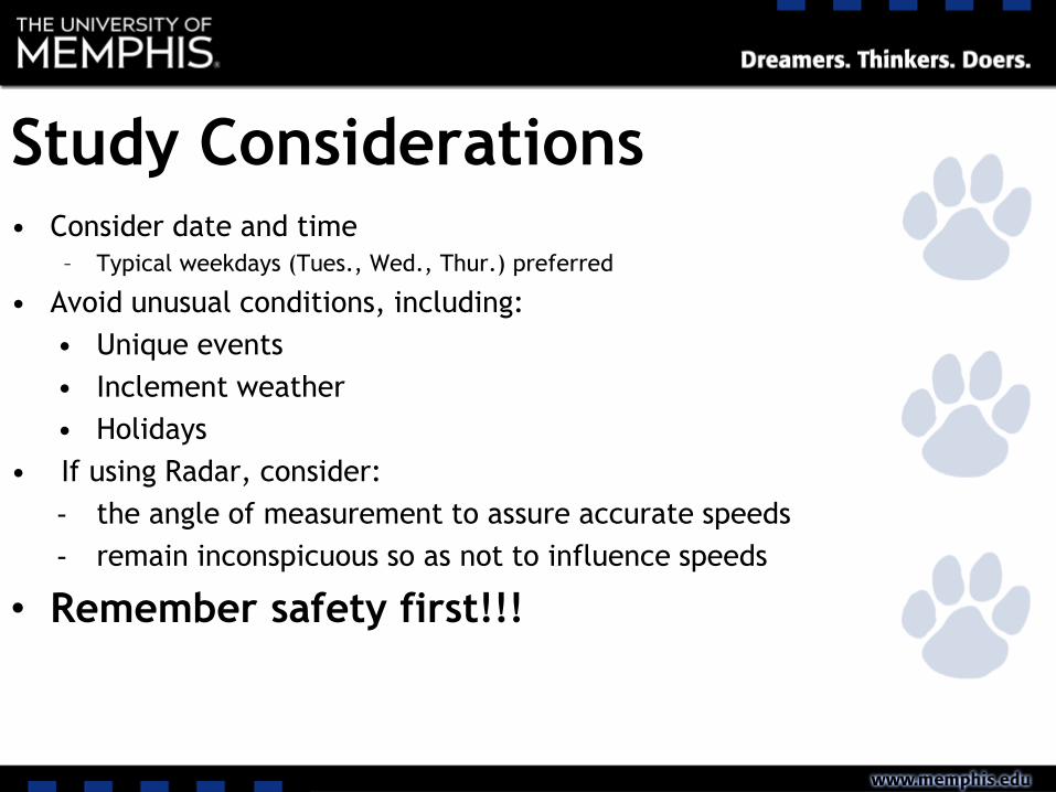
Study Considerations• Consider date and time

– Typical weekdays (Tues., Wed., Thur.) preferred

• Avoid unusual conditions, including:

• Unique events

• Inclement weather

• Holidays

• If using Radar, consider:

- the angle of measurement to assure accurate speeds

- remain inconspicuous so as not to influence speeds

• Remember safety first!!!

Spot Speed Study Analysis

• Data reduction (tabular and graphical

presentation)

• Descriptive statistics (mean, median,

mode, standard deviation, pace, etc.)

• Statistical inference (do significant

differences exist between mean speeds

for different conditions, etc.)

• A sample size of 100 veh per lane is

acceptable for most circumstances

Data presentation

• Frequency distribution

• Cumulative frequency distribution

• Indicate central tendency and

dispersion

• Evaluation depends on whether or not

individual speeds or speed classes

collected

Uninterrupted Flow Conditions• Sample Mean

• Sample Standard Deviation

• Where,• 𝜇 -> Sample mean speed, mph

• 𝜇𝑖->Speed of vehicle i, mph

• N->Total number of speed observations

• s2->Sample variance

• s->Sample standard deviation

𝜇 =σ𝑖=1𝑁 𝜇𝑖𝑁

𝑠2 =σ𝑖=1𝑁 𝜇𝑖 − 𝜇 2

𝑁 − 1

Grouped Observations• Sample Mean

• Sample Standard Deviation

• Where,

• 𝜇 -> Sample mean speed, mph

• 𝜇𝑖-> Speed of vehicle i, mph

• N-> Total number of speed observations

• s2-> Sample variance

• s-> Sample standard deviation

• fi-> Number of observations in speed group I

• g-> Number of speed groups

𝜇 =σ𝑖=1𝑔

𝑓𝑖𝜇𝑖𝑁

𝑠2 =σ𝑖=1𝑔

𝑓𝑖 𝜇𝑖2 −

1𝑁

σ𝑖=1𝑔

𝑓𝑖𝜇𝑖2

𝑁 − 1

Speed Exercise

Statistical inference

• Most speed data tends to follow

normal distribution

• This can be evaluated using chi-square

test for goodness of fit

• If the data is normally distributed,

confidence intervals may be

determined, and required sample sizes

may be estimated

Normal Distribution

• A unique normal distribution is defined when

mean and standard deviation are specified

• The normal distribution is

– Symmetrical about the mean

– Dispersion is a function of the standard deviation

Normal Distribution

𝜇1, 𝑠1

𝜇2, 𝑠2

𝜇3, 𝑠3

𝑠1 = 𝑠2, 𝑏𝑢𝑡 𝜇1 < 𝜇2𝜇2 = 𝜇3, but 𝑠2<𝑠3

Normal Distribution

• The dispersion is such that

– 68.27% of observations will be within 1 s.d

– 95.45% of observations will be within 2 s.d

– 99.73% of observations will be within 3 s.d

1 s.d = 68.27%

Two Issues with Normal Distribution

• Issue-1: Sample mean and sample s.d are

known for most studies; population mean and

population standard deviation are very

difficult to estimate

• Issue-2: Estimating population s.d from the

sample s.d is even more complex

Sample Size

• The relationship between sample and

population is N

• As N increases to infinite, then sample s.d is

equivalent to population s.d

• In practice it is found that

– If N>30, then sample s.d = mean s.d

– If N<30, then t-distribution rather than normal

distribution is used

Question• What is the probability of individual speeds

between 35 and 40 mph

• Probability value for 2.75, = 0.4970

• Probability value for 1.95, = 0.4744

• Probability of speed between 35 and 40 = 0.4970-0.4744 = 0.0226

• With sample size of 200, the expected frequency is 0.0226*200 = 4 or 5

𝑥

𝜎 35→52.3=

52.3−35.0

6.3=2.75

𝑥

𝜎 40→52.3=

52.3−40.0

6.3=1.95

Evaluation of Selected Mathematical

Distribution (1)• Rule-1: The variance of measured speed

distribution normally should be less than the variance of a random distribution (i.e. poisson)– s2=6.3^2 = 39.3 mph

– s2r= m = 52.3 mph

– s2 < s2r

• Rule-2: The s.d should be approximately 1/6th of total range since plus or minus 3 s.d encompasses 99.73% of the observations of a normal distribution

sest = total range/6 = 32/6 = 5.3 mph

s~ sest

Evaluation of Selected Mathematical

Distribution (2)• Rule-3: The standard deviation should be

approximately one half of the 15 to 85 percentage range– sest = (15 – 85 percentile range) / 2

– =12.3/2 = 6.15

– s~ sest

• Rule-4: The 10 mile per hour pace should be approximately equal to the sample mean– 10 mile hour pace= 52 or 53

– Mean = 52.3

– Pace ~ Mean

Evaluation of Selected Mathematical

Distribution (3)• Rule-5: The normal distribution has little

skewness and the coefficient of skewness

should be close to zero.

– Coeffieicent of skewness = mean-mode/s

– =52.3-53/6.3 = 0.1

Or

– 3[(mean-median)/s] = 3[(52.3-52.5)/6.3]=0.1

• The numerical checks appear to support the

assumption of a normal distribution

Testing for Normalcy

• Null Hypothesis: There is no statistical

difference between the measured distribution

and normal distribution

• Alternate Hypothesis: There exists statistical

difference between the measured distribution

and normal distribution

Testing for Normalcy: The Chi-Square

Test (1)• Group the data and find the estimated

frequencyClass Interval Limit z z/s P Pt Ft

0.0038 0.77

35.5 16.8 2.666667 0.4962 0.0104 2.08

38.5 13.8 2.190476 0.4858 0.0290 5.80

41.5 10.8 1.714286 0.4568 0.0646 12.92

44.5 7.8 1.238095 0.3922 0.1152 23.04

47.5 4.8 0.761905 0.2769 0.1645 32.90

50.5 1.8 0.285714 0.1125 0.1880 37.60

53.5 1.2 0.190476 0.0755 0.1720 34.40

56.5 4.2 0.666667 0.2475 0.1259 25.19

59.5 7.2 1.142857 0.3735 0.0738 14.77

62.5 10.2 1.619048 0.4473 0.0527 10.54

Testing for Normalcy: The Chi-Square

Test (2)

Class Interval Limit f0 ft f0-ft (f0-ft)^2 [(f0-ft)^2]/ft

4 0.766076

35.5 2 2.082896

38.5 4 5.798655 1.352373 1.828914 0.315403155

41.5 10 12.92045 -2.92045 8.529019 0.660117863

44.5 19 23.04361 -4.04361 16.35078 0.709558121

47.5 31 32.89801 -1.89801 3.602447 0.109503502

50.5 41 37.5967 3.403296 11.58242 0.308070208

53.5 40 34.39509 5.604908 31.41499 0.91335674

56.5 23 25.18872 -2.18872 4.79048 0.190183585

59.5 18 14.76609 3.233911 10.45818 0.708256568

62.5 8 10.5437 -2.5437 6.470419 0.61367619

Sum 4.528125932

Conclusion

• 𝜒2 from the table for = 0.05, and degrees of

freedom=6; is 12.6

• Since 𝜒2 calculated is less than the table

value, we fail to reject the hypothesis.

• The conclusion is

– There is no statistical difference between the

measured distribution and normal distribution

Sample size

• 𝑛 =𝑡𝑠

𝜖

2

• Where

– n-> required sample size

– t- coefficient of standard error that represents

user specified probability level

– 𝜖: user specified probable error

– s: standard deviation