Traffic Flow Characteristics

CIVL 4162/6162

(Traffic Engineering)

Lesson Objective

• Define traffic stream parameters

• Establish the relationship between traffic

stream parameters

• Calculate and compute parameters with given

data

What is a Traffic Stream

• Traffic streams are made up of

– Individual drivers

– Vehicles

– Roadway and environment

• Driver behavior and vehicle characteristics

typically vary

• No two traffic streams will behave exactly in

the same way

Variability in Traffic Stream (1)

• Traffic flow (movement of vehicles) involves

variability

– Unlike pipe flow (homogeneous)

• A given traffic flow will vary

– By time

– By space

• Constraints are defined by

– Physical constraints

– Complex driver characteristics

Variability in Traffic Stream (2)

• Although traffic characteristics vary there is a

reasonable range

– Example: In a 65 miles/hr roadway some drivers

will drive 50 miles/hr and some will drive 80

miles/hr

• There exists a range

• Before we study traffic characteristics let us

see what are

– Facilities

– Basic flow parameters

Types of Facilities• Uninterrupted Flow Facilities

– No external interruptions

– Primarily on freeways

– Also on certain segments of long rural highways

– In peak hours also freeways are uninterrupted

• Interrupted Flow Facilities

– External interruptions exists

– Most frequent are signals, stop/yield signs

– Creates platoons of vehicles progress in traffic

stream

Types of Facilities and Major Difference

• The major difference between two facilities

– Impact of time (no interventions at any time)

– Availability of roadways

• On uninterrupted facilities roadways are available to

users all the time

• But sections of roadway are not available to users

because of traffic control (signal, stop, and yield signs)

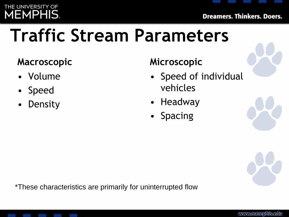
Traffic Stream Parameters

Macroscopic

• Volume

• Speed

• Density

Microscopic

• Speed of individual

vehicles

• Headway

• Spacing

*These characteristics are primarily for uninterrupted flow

Volume

• Traffic volume is defined as the number of

vehicles passing a point on highway or a given

lane or direction of a highway in a specific

time

• Unit: vehicles per unit time

• Usually expressed as vehicles / hour

• Denoted as veh/hr

Rate of Flow

• Rate of flow are generally expressed in units

of “veh/hr” but represents flows that exists

for period of time less than an hour.

• Example: 200 vehicles are observed for 15min.

• The equivalent hourly volume will be 800

veh/hr

• Even though 800 veh/hr would not be

observed if one hour was counted

Daily Volumes (1)

• Average Annual Daily Traffic (AADT) –

– The average 24 hour volume at a given location

over a full 365 day year.

– avg. 24-hour volume at a site over a full year

• Average Annual Weekday Traffic (AAWT) –

– The average 24 hour volume at a given location

occurring on weekdays over a full 365 day year.

– Usually 260 days week days per year

Daily Volumes (2)

• Average Daily Traffic (ADT) –

– The average 24 hour volume at a given location

over a defined time period less than a year

• Average Weekday Traffic (AWT)

– The average 24 hour weekday volume at a given

location over a defined period less than one year

Example: Daily Volume

Hourly Volume

• Measured in volume/hour

• Used for design and operational purposes

• The hour with highest volume is referred as

– Peak hour

• Peak hour volume is stated as directional

volume

• Sometimes referred as Directional Design

Hourly Volume (DDHV)

DDHV

• DDHV = directional design hourly volume

DDHV = AADT * K * D

where K = proportion of AADT that occurs

during design hour

D = proportion of peak hour traffic

traveling in the peak direction

K-Factor

• Typically, K factor represents proportion of AADT occurring

during 30th peak hour of the year

• How does K-factor vary by urban density?

– Urban, suburban, and rural

• D Factors

– More variable than K

– Influenced by development density, radial vs.

circumferential route

K and D Factor

Flow Rate vs. Volume

Volume vs. Flow Rate

If capacity is 4,200 vph:

Peak Hour Factor

• 15 minutes is considered to be minimum

period of time over which traffic can be

considered statistically stable

• Peak hour factor (PHF) represents the

uniformity of flow in the peak hour.

 

PHF =V

4 *Vm15

where :

V = hourly volume,vehs

Vm15 = max15min volume within the hour,vehs

Peak Hour Factor (2)

• PHF = 4200/(4*1200) = 0.875

Peak Hour Factor (3)

• Peak hour factor lie between 0.25-1

– 0.25 when all traffic is concentrated in one 15

minute period

– 1.0 when traffic on all 15 minute period are same

• Under very congested conditions PHF~1

• Practical studies show that

– PHF~0.7 for rural roadways

– PHF~0.98 in dense urban roadways

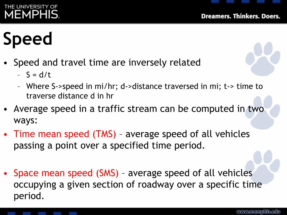
Speed

• Speed and travel time are inversely related

– S = d/t

– Where S->speed in mi/hr; d->distance traversed in mi; t-> time to

traverse distance d in hr

• Average speed in a traffic stream can be computed in two

ways:

• Time mean speed (TMS) – average speed of all vehicles

passing a point over a specified time period.

• Space mean speed (SMS) – average speed of all vehicles

occupying a given section of roadway over a specific time

period.

TMS and SMS

• Time Mean Speed (TMS)

• Space Mean Speed (SMS)

• Where

– d-> distance traversed, ft

– n-> number of observed vehicles

– ti->time for vehicle “i” to traverse the distance d

Example: TMS and SMS

Example: Time Mean vs Space Mean

Speed

Figure 5.1 Time Mean Speed and Space Mean Speed Illustrated

TMS = (88n+44n)/(2n) = 66 ft/sec

SMS = (88n+44*2n)/(3n) = 58.7ft/sec

Consider a long, uninterrupted, single-

lane roadway:

No passing, no opposing traffic,

no intersections

Traffic Flow Basics (1)

Time (t)

Dis

tance

(x)

Traffic Flow Basics (2)

Time (t)

Dis

tance

(x)

Dt

Dx

Traffic Flow Basics-Speed

Time (t)

Dis

tance

(x)

Traffic Flow Basics-Trajectories

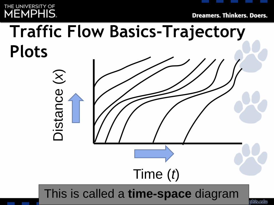
Time (t)

Dis

tance

(x)

This is called a time-space diagram

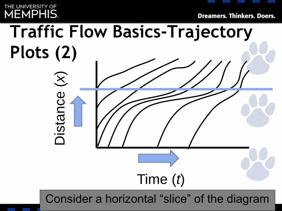
Traffic Flow Basics-Trajectory

Plots

Time (t)

Dis

tance

(x)

Consider a horizontal “slice” of the diagram

Traffic Flow Basics-Trajectory

Plots (2)

The number of trajectories crossing this line is the number of vehicles

passing a fixed point on the road.

Time (t)

Dis

tance

(x)

This is called the volume or flow, and has units of

vehicles per time (usually veh/hr)

Traffic Flow Basics-Volume

What does a vertical

slice tell us?Time (t)

Dis

tance

(x)

Traffic Flow Basics-Density

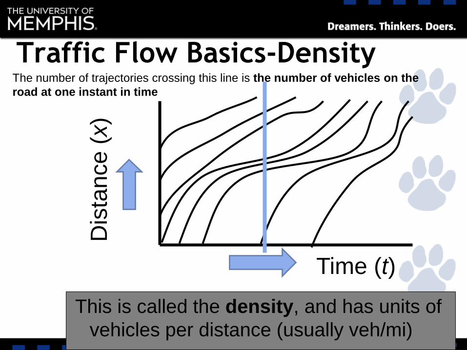
The number of trajectories crossing this line is the number of vehicles on the

road at one instant in time

Time (t)

Dis

tance

(x)

This is called the density, and has units of

vehicles per distance (usually veh/mi)

Traffic Flow Basics-Density

Density

• Most direct measure of traffic demand

• Difficult to measure directly

• Important measure of quality of traffic flow

• Occupancy is related, and can be measured directly

• Occupancy – proportion of time that a detector is

occupied by a vehicle in a defined time period.

Figure 5.2 Density and Occupancy Illustrated

Density and Occupancy