Civil Engineering – IISc Bangalore
280
Transcript of Civil Engineering – IISc Bangalore


��������������� �������������������������������� ���

About the Authors
Dr. S. Vedula obtained his Ph. D. from Colorado StateUniversity, USA in 1970, and served the New York StateDepartment of Environmental Conservation for three years.He joined the Indian Institute of Science (IISc), Bangalore,as a faculty member in 1972 in the Department of CivilEngineering, and served the Institute till his superannuationin 2001. Subsequently, he continued at IISc as a AICTEEmeritus Fellow till the end of 2003. His areas ofspecialization include water resources systems, reservoir
operations, irrigation planning and management. He is a recipient of BharatSingh Award, Pt. Jawaharlal Nehru Birth Centenary Research Award, andDr. C.M. Jacob Gold Medal by the Systems Society of India for his outstandingcontributions in Water Resources Systems and Hydrology.
During his tenure at the Indian Institute of Science, Bangalore, Dr. Vedulaworked as Senior Fellow at Harvard University, and as visiting faculty at theAsian Institute of Technology, Bangkok for a short while. He served as aconsultant to several state and central government organizations on large scalewater resources projects with special reference to systems modelling in reservoiroperations, irrigation management, and conjunctive use planning in canalcommand areas. He has been associated with several reputed institutions inhydrology and water resources in India as a member of their high level technicalcommittees.
Dr. P.P. Mujumdar is currently working as a Professorat the Indian Institute of Science (IISc), Bangalore. Aftercompleting his Ph. D. from IISc in 1989, he worked as afaculty member at IIT Bombay for three years beforejoining IISc as a faculty member in 1992. His area ofspecialization is Water Resources Systems Modelling witha focus on uncertainty modelling for river water qualitycontrol, and planning and operation of large scale waterresources systems. His major research contributions
include development of models and software tools to aid planning andoperational decisions using the mathematical techniques of stochastic dynamicprogramming, fuzzy optimization and fuzzy risk and reliability. He is currentlyserving as a Section Member of the Water Resources Management Section ofthe International Association for Hydraulic Research (IAHR). He has served asa member of the editorial board of the journal Water International, and hasbeen a member of several state and national committees dealing with operationaland environmental aspects of water resources in India. He is a recipient of theCBIP Young Engineer Award, and the Prof. Satish Dhawan State Award forEngineering Sciences. His areas of professional consultancy include river basinplanning, reservoir operations, lift irrigation, urban drainage, hydropowerdevelopment and impact assessment of water resources projects. The author
can be contacted at (http://civil.iisc.ernet.in/~pradeep).

Water Resources Systems
Modelling Techniques and Analysis
S Vedula Formerly, Professor,
Department of Civil Engineering Indian Institute of Science, Bangalore
P P Mujumdar
Professor, Department of Civil Engineering Indian Institute of Science, Bangalore

��������
Preface vii
Acknowledgements ix
PART ONE
BASICS OF SYSTEMS TECHNIQUES
1. Concept of System and Systems Analysis 3
1.1 Definition of a System 3
1.2 Types of Systems 3
1.3 Systems Approach 5
1.4 Systems Analysis 5
Reference 7
Further Reading 7
2. Systems Techniques in Water Resources 8
2.1 Optimization Using Calculus 9
2.2 Linear Programming 23
2.3 Dynamic Programming 61
2.4 Simulation 87
2.5 Combination of Simulation and Optimization 89
References 90
Further Reading 90
3. Economic Considerations in Water Resources Systems 91
3.1 Basics of Engineering Economics 91
3.2 Economic Analysis 102
3.3 Conditions of Project Optimality 107
3.4 Benefit Cost Analysis 114
References 122
Further Reading 122
4. Multiobjective Planning 123
4.1 Noninferior Solutions 124
4.2 Plan Formulation 125
4.3 Plan Selection 129
Reference 129
Further Reading 129

PART TWO
MODEL DEVELOPMENT
5. Reservoir Systems—Deterministic Inflow 133
5.1 Reservoir Sizing 133
5.2 Reservoir Operation 148
Reference 165
Further Reading 165
6. Reservoir Systems—Random Inflow 166
6.1 Review of Basic Probability Theory 166
6.2 Chance Constrained Linear Programming 176
6.3 Concept of Reliability 188
6.4 Stochastic Dynamic Programming for Reservoir Operation 193
References 204
Further Reading 204
PART THREE
APPLICATIONS
7. Applications of Linear Programming 207
7.1 Irrigation Water Allocation for Single and Multiple Crops 207
7.2 Multireservoir System for Irrigation Planning 215
7.3 Reliability Capacity Tradeoff for Multicrop Irrigation 221
7.4 Reservoir Operation for Irrigation 224
7.5 Reservoir Operation for Hydropower Optimization 228
References 233
Further Reading 234
8. Applications of Dynamic Programming 235
8.1 Optimal Crop Water Allocation 235
8.2 Steady State Reservoir Operating Policy for Irrigation 236
8.3 Real-time Reservoir Operation for Irrigation 240
References 242
Further Reading 242
9. Recent Modelling Tools 244
9.1 Artificial Neural Networks 244
9.2 Fuzzy Sets and Fuzzy Logic 249
9.3 Fuzzy Linear Programming 257
References 272
Further Reading 274
Index 276
�� Contents

�����
A curriculum in water resources in teaching institutions across the country
invariably contains at least one course on Water Resources Systems, which
essentially deals with modelling techniques for optimum utilization of available
water resources. Excellent books are available today, which specialize
exclusively on individual topics of the course curriculum, such as linear
programming, dynamic programming, and stochastic optimization with
applications. However, a single book that caters to the needs of students entering
the subject area, emphasizing the basics of systems techniques in water resources
with illustrative examples, and potential applications to real systems, is preferable
for classroom teaching. Also, most of the books available in the market are out
of the affordable range of the students. These considerations motivated us in
our attempt to bring out the book in this form.
The contents of the book are organized in three parts—Part One: Basics of
Systems Techniques; Part Two: Model Development; and Part Three:
Applications.
Part One presents the basic techniques necessary in water resources systems
modelling. Chapter One gives a brief account of the concept of systems and
systems analysis. The core part of optimization techniques is presented in
Chapter Two. Basics of optimization using calculus, Linear Programming (LP)
and Dynamic Programming (DP), and a brief account of simulation are covered
in it. Chapter Three details the basic concepts of engineering economics.
Microeconomics, price theory, demand curves, aggregation of demand,
conditions of optimality in a production process, benefit and cost considerations,
and evaluation of engineering alternatives are covered in this chapter. A brief
account of multiobjective analysis is presented in Chapter Four, illustrating the
basics of weighting and constraint methods of generating noninferior solutions
to a multiobjective optimization problem.
Part Two illustrates the basic techniques in formulating models for selected
problems in reservoir systems with deterministic as well as stochastic inputs. In
Chapter Five models for reservoir sizing and operation, and reservoir simulation
for hydropower production are discussed in the deterministic domain.
Randomness of inflow is dealt with in Chapter Six, illustrating chance
constrained linear programming and stochastic dynamic programming
applications in reservoir operation.

Part Three presents a number of specific applications in reservoir systems
modelling including recently developed tools: ANN and Fuzzy sets. Chapter
Seven presents linear programming applications to crop yield optimization,
reliability capacity relationships, multiobjective analysis of multireservoir system,
short term reservoir operation, and reservoir operation for hydropower
optimization. Dynamic programming is applied to optimal crop water allocation,
derivation of steady state reservoir operating policy and real time operation in
Chapter Eight. Chapter Nine introduces the basics of recent modelling tools—
ANNs and Fuzzy sets. Applications illustrated include inflow forecasting using
ANN, Fuzzy rule-based reservoir operation, and Fuzzy LP for river water
quality management and reservoir operation. In the applications discussed in
Part Three, model formulations of examples and case studies are presented
without questioning the assumptions made in them, some of which may need
explanation beyond the scope of the book. The aim is essentially to introduce
the reader to the articulations in model formulation in a given situation with
appropriate assumptions.
We have extensively used the contents of the first two parts of the book for
teaching postgraduate students at Indian Institute of Science, Bangalore. Selected
sections of the book may be used as teaching material for students at different
levels: Part One to introduce the basics, Part Two to impart training to acquire
skills in modelling, and Part Three to help articulation of model formulations to
practical problems. Part One will in itself form the core contents of a
2-credit course in water resources systems in one semester. The course material
may be supplemented by selected topics from Part Two, especially Chapter 5.
A regular 3-credit course may include Parts One and Two. A term paper or a
seminar may be included as a part of the syllabus, for which the contents of
Part Three should aid students in selecting topics of individual interest. Graduate
research students will find Part Three, in which a range of applications are
illustrated, useful in selecting topics for further study or in generating additional
skills for wider applications of systems modelling.
Over the past two and half decades, a large number of our students, endured
our presence in the classroom and helped us learn with them. We thank them
for helping us crystallize our thoughts over years in bringing out this book. We
acknowledge here that we have been highly inspired by the classical book,
“Water Resources Systems Planning and Analysis” by Loucks et al. (1981),
which stimulated us to bring out this book in the present form.
Needless to say, in a maiden attempt of this kind, we might have inadvertently
erred on some counts. We appeal to all readers, colleagues and students, to
point out these, and to offer constructive suggestions for improving the book.
S VEDULA
P P MUJUMDAR
���� Preface

�� �������������
The authors thank the Centre for Continuing Education (CCE), Indian Institute
of Science (IISc), Bangalore for its financial support in the preparation of the
manuscript of the book. The help rendered by the graduate students of the
Department of Civil Engineering, IISc in editing the manuscript is also gratefully
acknowledged.

���� �
������������� �����������
� Concept of System and Systems Analysis
� Systems Techniques in Water Resources
� Economic Considerations in Water Resources Systems
� Multiobjective Planning

������� �
�������������� ������� ���������
his chapter deals with the definition of a system, factors governing a
system, system analysis, typical problems associated with systems and a
brief account of the techniques used to solve these problems. The concept of
systems analysis is indeed very wide, but we shall confine our discussion in
this section to a typical hydrological/water resources system.
��� ������������ ����
The basic concept of a system is that it relates two or more things. Out of the
several definitions of a system, the simplest one states that it is a device that
accepts one or more inputs and generates one or more outputs. A comprehen-
sive definition of a system is given by Dooge (Dooge, 1973) as “any structure,
device, scheme, or procedure, real or abstract, that interrelates in a given time
reference, an input, cause, or stimulus, of matter, energy, or information, and
an output, effect or response, of information, energy or matter.” The input and
output referred to in mechanics is synonymous with cause and effect in physics
and philosophy, and stimulus and response in biological sciences.
Typical examples of a system are a university with its various departments, a
central government with its regional governments, a river basin with all its
tributaries, and so on.
��� � ����� �����
Some commonly understood types of systems are discussed as below.
��������������� ��������
A simple system is one in which there is a direct relation between the input and
the output of the system. A complex system is a combination of several sub-
systems each of which is a simple system. Therefore, a complex system may be
subdivided into a number of simple systems. Each subsystem has a distinct
relation between input and output. For example, a river basin system is a
T

� Basics of Systems Techniques
complex system comprising several subsystems, each corresponding to a tribu-
tary.
�����������������������
A linear system is one in which the output is a constant ratio of the input. In a
linear system the output due to a combination of inputs is equal to the sum of
the outputs from each of the inputs individually, i.e. the principle of superposi-
tion is valid. For example, a system (watershed) in which the input x (rainfall)
and the output y (runoff) are related by y = mx, in which m is a constant, is a
linear system. The unit hydrograph in hydrology is a linear system (as the
hydrograph ordinate of the direct runoff hydrograph is proportional to the
rainfall excess). On the other hand, a system in which the input x and the
output y are related by the linear equation y = mx + c, in which m and c are
constants, is not a linear system (why?). A nonlinear system is one in which the
input–output relation is such that the principle of superposition is not valid. In
reality, a watershed is a nonlinear system, as the runoff from the watershed due
a storm is a nonlinear function of the (storm) rainfall over its area.
����������������������������������
In a time invariant system, the input–output relationship does not depend on
the time of application of the input, i.e. the output is the same for the same
input at all times. The unit hydrograph in hydrology is a linear time invariant
system.
������������������������������������
In a continuous system, the changes in the system take place continuously;
whereas in a discrete system, the state of the system changes at discrete inter-
vals of time. A variable, input or an output, is said to be quantized when it
changes only at certain discrete intervals of time and holds a constant value
between intervals (e.g. rainfall record).
����������������������������������������������
A lumped parameter is one whose variation in space is either nonexistent or
ignored (e.g. average rainfall over a watershed). A parameter is said to be a
distributed one if its variation in one or more spatial dimensions is taken into
account. The parameters of the system, the input or the output may be lumped.
A lumped parameter system is governed by ordinary differential equations
(with time as an independent variable), whereas a distributed parameter system
is governed by partial differential equations (with spatial coordinates as inde-
pendent variables). For example, a homogeneous isotropic aquifer is analyzed
as a lumped parameter system. Instead, if the spatial variation of the
transmissivity in modelling a water table aquifer is to be taken into account, the
aquifer has to be modelled as a distributed parameter system.

Concept of System and Systems Analysis �
������������������������������������
In a deterministic system, if the input remains the same, the output remains the
same, i.e. the same input will always produce the same output. The input itself
may be deterministic or stochastic. In a probabilistic system, the input–output
relationship is probabilistic rather than deterministic. The output corresponding
to a given input will have a probability associated with it.
��������������
A stable system is one in which the output is bounded if the input is bounded.
Virtually all systems in hydrology and water resources are stable systems.
��� � ������������
The input–output relationship of a system is controlled by the nature, param-
eters of the system and the physical laws governing the system. In many of the
systems in practice, the nature and the principal laws are very complex, and
systems modelling in such cases uses simplifying assumptions and transforma-
tion functions, which convert the input to the corresponding output, ignoring
the mechanics of the physical processes involved in the transformation. This
requires conceptualization of the system and its configuration to be able to
construct a mathematical model of it in which the input–output relationships
are established through operating the system in a defined fashion. The specifi-
cation of the system operation is what we refer to as the operating policy.
��� � ��������� ���
Systems analysis may be said to be a formalization of the operation of the total
system with all of its subsystems together. Systems analysis is usually understood
as a set of mathematical planning and design techniques, which includes some
formal optimization procedure. When scarce resources must be used effectively,
systems analysis techniques stand particularly promising (for example, in optimal
crop water allocation to several competing crops, under conditions of limited
water supply). It must be clearly understood that systems analysis is not merely
an exercise in mathematical modelling but spans much farther into processes
such as design and decision. The techniques may use both descriptive as well
as prescriptive models. The descriptive models deal with the way the system
works, whereas the prescriptive ones are aimed at deciding how the system
should be operated to best achieve the specified objectives.
����� ��������� !"��#�$�%!"��#� $���
Basically there are two types of problems: analysis and synthesis. The first one
is essentially a problem of prediction or a direct problem, whereas the second
is a problem of identification or an inverse problem. In a prediction problem,
we are required to determine the output knowing the input and the system
operation. In an inverse problem, we are required to find the system (parameters),
given the input and the output. In synthesis, we devise a model (system) that

& Basics of Systems Techniques
will convert a known input to its corresponding known output. Here, we have
to keep in mind the nature of the system and its operation.
����� �'�"( !���� !"�
Prediction In surface water hydrology, the problem is to predict the storm
runoff (output), knowing the rainfall excess (input) and the unit hydrograph
(system). In ground water hydrology, the problem is to determine the response
(output) of a given aquifer (system), for given rainfall and irrigation application
(input). In a reservoir (system) the problem is to determine irrigation alloca-
tions (output) for given inflow and storage (input), based on known or given
operating policy.
Identification In surface water hydrology, the problem is to derive the unit
hydrograph (system) given precipitation (input) and runoff data (output) for the
concurrent period. It is assumed that all the complexities of the watershed
including the geometry and physical processes in the runoff conversion are
described by the unit hydrograph. In ground water hydrology, the problem is to
determine the aquifer parameters (system), given the aquifer response (output)
for known rainfall and irrigation application (input).
In a reservoir system, the problem is to determine the reservoir release
policy (system operation) for a specified objective (output) for given inflows a
(input).
Synthesis The problem of synthesis is even more complex than the inverse
problem mentioned earlier. Here no record of input and output are available.
An example is the derivation of Snyder’s synthetic unit hydrograph using
watershed characteristics to convert known values of rainfall excess to runoff.
����� �!�)#�*+!��,-�%!��!��+��!��$�%!"��#� $���
The basic techniques used in water resources systems analysis are optimization
and simulation. Whereas optimization techniques are meant to give global
optimum solutions, simulation is a trial and error approach leading to the
identification of the best solution possible. The simulation technique cannot
guarantee global optimum solution; however, solutions, which are very close to
the optimum, can be arrived at using simulation and sensitivity analysis.
Optimization models are embodied in the general theory of mathematical
programming. They are characterized by a mathematical statement of the ob-
jective function, and a formal search procedure to determine the values of
decision variables, for optimizing the objective function. The principal optimi-
zation techniques are:
1. Linear Programming The objective function and the constraints are all
linear. It is probably the single-most applied optimization technique the world
over. In integer programming, which is a variant of linear programming, the
decision variables take on integer values. In mixed integer programming, only
some of the variables are integers.

Concept of System and Systems Analysis .
2. Nonlinear Programming The objective function and/or (any of) the con-
straints involve nonlinear terms. General solution procedures do not exist. Spe-
cial purpose solutions, such as quadratic programming, are available for limited
applications. However, linear programming may still be used in some engineer-
ing applications, if a nonlinear function can be either transformed to a linear
function, or approximated by piece-wise linear segments.
3. Dynamic Programming Offers a solution procedure for linear or nonlin-
ear problems, in which multistage decision-making is involved.
The choice of technique for a given problem depends on the configuration
of the system being analyzed, the nature of the objective function and the
constraints, the availability and reliability of data, and the depth of detail needed
in the investigation. Linear programming (LP), and dynamic programming (DP)
are the most common mathematical programming models used in water re-
sources systems analysis. Simulation, by itself, or in combination with LP, DP,
or both LP and DP is used to analyze complex water resources systems.
���������
1. Dooge, J. C. I., ‘‘Linear Theory of Hydrologic Systems’’, Technical Bulle-
tin No. 1468, Agricultural Research Service, US Department of Agricul-
ture, 1973.
1. Ossenbruggen, P. J., Systems Analysis for Civil Engineers, John Wiley &
Sons, New York, 1984.

I
������� �
������������ ��������������������
n most engineering problems, decisions need to be made to optimize (i.e.
minimize or maximize) an appropriate physical or economic measure. For
example, we may want to design a reservoir at a site with known inflows for
meeting known water demands, such that the reservoir capacity is minimum, or
we may be interested in locating wells in a region such that the aquifer draw-
down is minimum for a given pumping pattern. Most engineering decision-
making problems may be posed as optimization problems. In general, an opti-
mization problem consists of:
(a) an objective function, which is a mathematical function of decision vari-
ables, that needs to be optimized, and
(b) a set of constraints that represents some physical (or other) conditions to
be met.
The decision variables are the variables for which decisions are required
such that the objective function is optimized subject to the constraints. In the
first example mentioned, the reservoir capacity is one of the decision variables
and the reservoir mass balance defines one set of constraints. In the second
example, the locations—in terms of coordinates—of the wells are the decision
variables, and again, the mass balance forms a set of constraints.
A general optimization problem may be expressed mathematically as
Maximize f(X)
subject to
gj (X) � 0 j = 1, 2, … m
where, X is a vector of decision variables, X = [x1, x2, x3, …. xn]. In this
general problem there are n decision variables (viz. x1, x2, x3, …. xn) and m
constraints. The complexity of the problem varies depending on the nature of
the function f(X), the constraint functions gj (X) and the number of variables
and constraints.
Simulation is a technique by which we imitate the behavior of a system.
Typically, we use simulation to answer ‘what-if’ type of questions. As against

Systems Techniques in Water Resources �
optimization, where we are typically looking for the ‘best possible’ solution, in
simulation we simply look at the behavior of the system for given sets of
inputs. Simulation is a very powerful technique in analyzing most complex
water resource systems in detail for performance evaluation, while optimiza-
tion models yield results helpful in planning and management of large systems.
In some situations, optimization models cannot be even applied due to compu-
tational limitations. In many situations, however, decision-makers would be
interested in examining a number of scenarios rather than just looking at one
single solution that is optimal. Typical examples where simulation is used in
water resources include:
(a) analysis of river basin development alternatives,
(b) multireservoir operation problems,
(c) generating trade-offs of water allocations among various uses such as hy-
dropower, irrigation, industrial and municipal use, etc., and
(d) conjunctive use of surface and ground water resources.
It may be noted that by repeatedly simulating the system with various sets of
inputs it is possible to obtain near-optimal solutions.
In this chapter, an introduction to classical optimization using calculus is
presented first (Section 2.1), followed by the two most commonly used optimi-
zation techniques, Linear Programming (Section 2.2) and Dynamic Programming
(Section 2.3). An introduction to simulation is provided next (Section 2.4).
Applications of these techniques to water resources problems are discussed in
Part 2 of the book.
��� ���������� ����� ��������
Some basic concepts and rules of optimization of a function of a single vari-
able and a function of multiple variables are presented in this chapter.
����� �������� �� � ������ �� ��!��
Let f (x) be a function of a single variable x, defined in the range a < x < b
(Fig. 2.1).
f x( )
a x1 x2 x3 x4 x5 bx
���� ��� ���������������� ������ �
Local Maximum The function f (x) is said to have a local maximum at x1 and
x4, where it has a value higher than that at any other value of x in the
neighbourhood of x1 and x4. The function is a local maximum at x1, if
f(x1 – �x1) < f(x1) > f(x1+ �x1)

�" Basics of Systems Techniques
Local Minimum The function f(x) is said to have a local minimum at x2 and
x5, where it has a value lower than that at any other value of x in the
neighborhood of x2 and x5.
The function is a local minimum at x2, if
f(x2 – �x2) > f (x2) < f(x2 + �x2)
Saddle Point The function has a saddle point at x3, where the value of the
function is lower on one side of x3 and higher on the other, compared to the
value at x3. The slope of the function at x3 is zero.
f(x3 – �x3) < f (x3) < f (x3 + �x3); slope of f(x) at x = x3 is zero
Global Maximum The function f(x) is a global maximum at x4 in the range a
< x < b, where the value of the function is higher than that at any other value of
x in the defined range.
Global Minimum The function f(x) is a global minimum at x2 in the range a
< x < b, where the value of the function is lower than that at any other value of
x in the defined range.
��������A function is said to be strictly convex, if a straight line connecting any two
points on the function lies completely above the function. Consider the func-
tion f (x) in Fig. 2.2.
f (x) is said to be convex if the line AB is completely above the function
(curve AB). Note that the value of x for any point in between A and B can be
expressed as �x1 + (1 – �)x2, for some value of �, such that 0 � � � 1.
Therefore,
f(x) is said to be strictly convex if
f [�x1 + (1 – � ) x2] < � f (x1) + (1 – � ) f(x2); where 0 � � � 1
1. If the inequality sign < is replaced by � sign, then f(x) is said to be convex,
but not strictly convex.
2. If the inequality sign < is replaced by = sign, f (x) is a straight line and
satisfies the condition for convexity mentioned in 1 above. Therefore, a
straight line is a convex function.
���� ��� ���������������
Systems Techniques in Water Resources ��
3. If a function is strictly convex, its slope increases continuously, or
2
2
d f
dx > 0. For a convex function, however,
2
2
d f
dx � 0.
�������
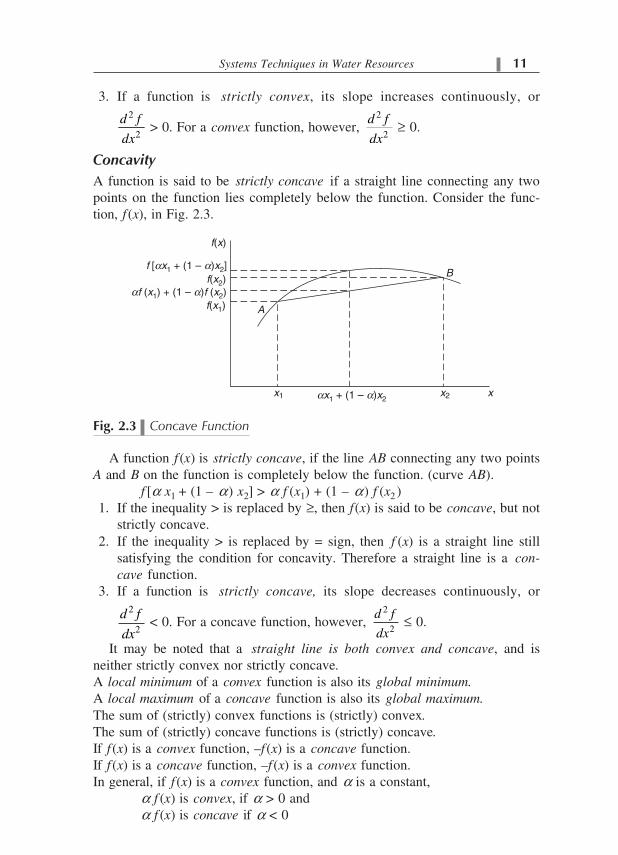
A function is said to be strictly concave if a straight line connecting any two
points on the function lies completely below the function. Consider the func-
tion, f (x), in Fig. 2.3.
A function f (x) is strictly concave, if the line AB connecting any two points
A and B on the function is completely below the function. (curve AB).
f [� x1 + (1 – � ) x2] > � f (x1) + (1 – � ) f (x2 )
1. If the inequality > is replaced by �, then f(x) is said to be concave, but not
strictly concave.
2. If the inequality > is replaced by = sign, then f (x) is a straight line still
satisfying the condition for concavity. Therefore a straight line is a con-
cave function.
3. If a function is strictly concave, its slope decreases continuously, or
2
2
d f
dx < 0. For a concave function, however,
2
2
d f
dx � 0.
It may be noted that a straight line is both convex and concave, and is
neither strictly convex nor strictly concave.
A local minimum of a convex function is also its global minimum.
A local maximum of a concave function is also its global maximum.
The sum of (strictly) convex functions is (strictly) convex.
The sum of (strictly) concave functions is (strictly) concave.
If f (x) is a convex function, –f (x) is a concave function.
If f (x) is a concave function, –f (x) is a convex function.
In general, if f (x) is a convex function, and � is a constant,
� f (x) is convex, if � > 0 and
� f (x) is concave if � < 0
���� ��# ���������������

�� Basics of Systems Techniques
����� �$��%�&����� �� � �������� �� � ������ �� ��!��
The point at which a function will have a maximum or minimum is called a
stationary point. A stationary point is a value of the independent variable at
which the slope of the function is zero.
x = x0 is a stationary point if
0x
df
dx = 0. This is a necessary condition for f (x)
to be a maximum or minimum at x0.
Sufficiency condition is examined as follows:
1. If 2
2
d f
dx > 0 for all x, f (x) is convex and the stationary point is a global
minimum.
2. If 2
2
d f
dx < 0 for all x, f (x) is concave and the stationary point is a global
maximum.
3. If 2
2
d f
dx = 0, we should investigate further.
In case of 3, find the first nonzero higher order derivative. Let this be the
derivative of nth order.
Thus, at the stationary point, x = x0,
n
n
d f
dx� 0
1. If n is even, x0 is a local minimum or a local maximum.
If
0
n
n
x
d f
dx> 0, x0 is a local minimum
If
0
n
n
x
d f
dx< 0, x0 is a local maximum
2. If n is odd, x0 is a saddle point.
����# �������� �� ����$�� �� ��!��'
Let f(X) be a function of n variables represented by the vector X = (x1, x2,
x3, … , xn). Before coming to the criteria for convexity and concavity of
a function of multiple variables, we should know the Hessian matrix (or
H-matrix, as it is sometimes referred to) of the function. The Hessian matrix,
H [f(X)], of the function, f (X), is defined as

Systems Techniques in Water Resources �#
H [ f (X )] =
2 2 2
21 2 11
2 2 2
22 1 22
2 2 2
21 2
( ) ( ) ( )
( ) ( ) ( )
( ) ( ) ( )
n
n
n n n
f X f X f X
x x x xx
f X f X f X
x x x xx
f X f X f X
x x x x x
� �� � �� � � � ��
� � �� � � � ��
� � �
� � � � � � � �
� � �
The convexity and concavity of a function of multiple variables is determined
by an examination of the eigen values of its Hessian matrix.
The eigen values of H [f(X)] are given by the roots of the characteristic
equation,
|� I – H [f(X)]| = 0
where I is an identity matrix, and � is the vector of eigen values. The function
f(X) is said to be positive definite if all its eigen values are positive, i.e. all the
values of � should be positive. Similarly, the function f (X) is said to be negative
definite if all its eigen values are negative, i.e. all the values of � should be
negative.
Convexity and Concavity If all eigen values of the Hessian matrix are posi-
tive, the function is strictly convex.
If all the eigen values of the Hessian matrix are negative, the function is
strictly concave.
If some eigen values are positive and some negative, or if some are zero, the
function is neither strictly convex nor strictly concave.
����( �$��%�&����� �� � �������� �� ����$�� �� ��!��'
���� ��������������������
Let f (X) be a function of multiple variables, X = (x1, x2, x3, …, xn).
A necessary condition for a stationary point X = X0 is that each first partial
derivative of f(X) should equal zero.
1 2 n
df df df
dx dx dx � = 0.
Whether the function is a minimum or maximum at X = X0 depends on the
nature of the eigen values of its Hessian matrix evaluated at X0.
1. If all eigen values are positive at X0, X0 is a local minimum. If all eigen
values are positive for all possible values of X, then X0 is a global mini-
mum.
2. If all eigen values are negative at X0, X0 is a local maximum. If all eigen
values are negative for all possible values of X, then X0 is a global maxi-
mum.
3. If some eigen values are positive and some negative or some are zero, then
X0 is neither a local minimum nor a local maximum.

�( Basics of Systems Techniques
)*�%$�� ����� Examine the following functions for convexity/concavity and
determine their values at the extreme points.
1. f(X) = 2 21 2x x� – 4x1 – 2x2 + 5
First determine the Hessian Matrix.
1
f
x
��
= 2x1 – 4,2
21
f
x
�
� = 2
2
f
x
��
= 2 x2 – 2;2
22
f
x
�
�= 2
2
1 2
f
x x
�� �
= 0, 2
2 1
f
x x
�� �
= 0
Therefore, H f(X) = 2 0
0 2
� � � �
Eigen values of H are obtained by
|�I – H| = 0
i.e. |�I – H| =2 0
0 2
��
��
= 0
or (� – 2)2 = 0
The eigen values are �1 = 2, � 2 = 2.
As both the eigen values are positive, the function is a convex function
(strictly convex). Also, as the eigen values do not depend on the value
of x1 or x2, the function is strictly convex.
The stationary points are given by solving
1
f
x
��
= 2x1 – 4 = 0
and2
f
x
��
= 2x2 – 2 = 0
i.e. x1 = 2, x2 = 1 or X = (2, 1).
Therefore the function f (X) has a global minimum at X = (2, 1).
2. f (X) = 2 21 2x x� � – 4x1 – 8
1
f
x
��
= –2x1 – 42
21
f
x
�
� = –2
2
f
x
��
= –2x2
2
22
f
x
�
� = –2

Systems Techniques in Water Resources �+
2
1 2
f
x x
�� �
= 0, 2
2 1
f
x x
�� �
= 0
H = 2 0
0 2
�� � �� �
|�I – H| = 2 0
0 2
��
��
= 0 or (� + 2)2 = 0
The Eigen values are � 1= –2, �2 = –2.
Both Eigen values of H Matrix are negative and are independent of
the value of x1 and x2. Therefore f(X) is a strictly concave function.
Stationary Point:1
f
x
��
= –2x1 – 4 = 0, x1 = –2
2
f
x
��
= –2x2 = 0, x2 = 0
That is X = (–2, 0) and is a global maximum.
The function f (X) has a global maximum at X = (–2, 0) equal to –4.
3. f(X ) = 3 31 2x x� – 3x1 – 12x2 + 20
1
f
x
��
= 213 3x �
2
21
f
x
�
�= 6x1
2
f
x
��
= 223 12x �
2
22
f
x
�
�= 6x2
2
1 2
f
x x
�� �
= 02
2 1
f
x x
�� �
= 0
H = 1
2
6 0
0 6
x
x
� � � �
Eigen values are given by the equation
|� I – H| = 0 or 1
2
6 0
0 6
x
x
�
�
�� � �� �
= 0
or (� – 6x1)(� – 6x2) = 0
Therefore �1 = 6x1, �2 = 6x2
That is, if both x1 and x2 are positive, then both eigen values are
positive, and f (X) is convex; or if both x1 and x2 are negative, then both
eigen values are negative, and f (X) is concave.

�, Basics of Systems Techniques
Stationary points:
1
f
x
��
= 213 3x � = 0, x1 = ±1
2
f
x
��
= 223 12x � = 0, x2 = ±2
Therefore,
(i) f(X) has a local minimum at (x1, x2) = (1, 2), equal to 13 + 23 – 3 (1)
– 12 (2) + 20 = 2. fmin(X ) = 2 at X = (1, 2).
(ii) f(X) has a local maximum at (x1, x2) = (–1, –2) equal to (–1)3
+ (–2)3 – 3 (–1) – 12 (–2) + 20 = 38. fmax(X ) = 38 at X = (–1, –2).
At the points (1, –2) and (–1, 2), the function is neither convex nor
concave. They are saddle points.
��� ��������������������
We shall discuss in this section the conditions under which a function of
multiple variables will have a local maximum or a local minimum, and those
under which its local optimum also happens to be its global optimum. Let us
first consider a function with equality constraints.
1. Function f (X) of n Variables with a Single Equality Constraint
Maximize or Minimize f (X)
Subject to g(X ) = 0
Note that f (X ) and g(X ) may or may not be linear.
We shall write down the Lagrangean of the function f (X) denoted by
Lf (X, �), and apply the Lagrangean multiplier method.
Lf (X ) = f (X ) – �g(X ), where � is a Lagrangean multiplier.
When g(X ) = 0, optimizing Lf (X ) is the same as optimizing f (X ). The
original problem of constrained optimization is now transformed into an un-
constrained optimization problem (through the introduction of an additional
variable, the Lagrangean multiplier).
If more than one equality constraint is present in the problem,
Maximize or Minimize f (X )
Subject to gp(X ) = 0, p = 1, 2, …, m
the Lagrangean function of f (X ) in this case is
Lf (X, �) = f (X ) – � 1 g1(X ) – �2 g2(X) – …, –�m gm(X )
where � = (�1, �2, …, �m)
A necessary condition for the function to have a maximum or minimum is
that the first partial derivatives of the function L should be equal to zero,
i
dL
dx= 0, i = 1, 2, …, n
p
dL
d�= 0, p = 1, 2, …, m

Systems Techniques in Water Resources �-
The (n + m) simultaneous equations are solved to get a solution, (X0, �0).
Let the second partial derivatives be denoted by
kij =2
i j
L
x x
�� �
evaluated at X 0, for i = 1, 2,…, n; j = 1, 2, …, n
hpi = ( )p
i
g X
x
�
�, evaluated at X 0, p = 1, 2, …, m
The sufficiency condition is specified below.
Consider the determinant D, denoted as |D|, given by
|D| =
11 12 1 11 1
21 22 2 12 2
1 2 1
11 12 1
1 2
0 0
0 0
n m
n m
m m nn n mn
n
m m mn
k k k h h
k k k h h
k k k h h
h h h
h h h
�
�
�
� � �� � �
� � �� �
� �
� � � � �
� � � � �
This is a polynomial in � of order (n – m) where n is the number of variables
and m is the number of equality constraints. If each root of � in the equation
|D| = 0 is negative, the solution X 0 is a local maximum. If each root is positive,
then X 0 is a local minimum. If some roots are positive and some negative, X 0 is
neither a local maximum nor a local minimum. Also, if all the roots are negative
and independent of X, then X 0 is the global maximum. If all the roots are
positive and independent of X, then X 0 is the global minimum.
)*�%$�� �����
Maximize f (X) = 2 21 2x x� �
Subject to x1 + x2 = 4 or x1 + x2 – 4 = 0
Solution:
g(x) = x1 + x2 – 4 = 0
The Lagrangean is
Lf ( X, �) = 2 21 2� �x x – � (x1 + x2 – 4)
At the stationary point,
1
��
L
x= –2x1 – � = 0
2
��
L
x= –2x2 – � = 0
�
��
L = –(x1 + x2 – 4) = 0

�. Basics of Systems Techniques
These equations yield x1 = x2 = 2, � = –4.
Now we shall determine if this is a maximum.
k11 = 2
21
�
�
L
x = –2, k12 =
2
1 2
�� �
L
x x = 0
k21 = 2
2 1
�� �
L
x x = 0, k22 =
2
22
�
�
L
x = –2
h11 = 1
��
g
x =1, h12 =
2
��
g
x = 1
|D| =
2 0 1
0 2 1
1 1 0
�
�
� �� � = 0
or 2� + 4 = 0 giving � = –2.
As the only root is negative, the stationary point X = (2, 2) is a local maxi-
mum of f (X) and fmax (X) = –8.
2. Function f(X) with Inequality Constraints An inequality constraint can
be converted to an equality constraint by introducing an additional variable on
the left-hand side of the constraint.
Thus a constraint g(X) � 0 is converted as g(X) + s2 = 0, where s2 is a non-
negative variable (being square of s). Similarly, a constraint g(X) � 0 is converted
as g(X) – s2 = 0.
The solution is found by the Lagrangean multiplier method, as indicated,
treating s as an additional variable in each inequality constraint.
When the Lagrangean of f(X) is formed with either type of constraint,
equating the partial derivative with respect to (w.r.t.) s gives,
�s = 0, meaning either � = 0 or s = 0.
1. If � > 0, s = 0. This means that the corresponding constraint is an equality
constraint (binding constraint or active constraint).
2. If s 2 > 0, � = 0. This means that the corresponding constraint is inactive or
redundant.
��������������������
The conditions mentioned above lead to the statement of Kuhn-Tucker
conditions. These conditions are necessary for a function f(X) to be a local
maximum or a local minimum. The conditions for a maximization problem are
given below.
Maximize f (X)
subject to g j (X) � 0, j = 1, …, m.
The conditions are as follows:

Systems Techniques in Water Resources ��
1
( )( ) mj
ji ij
g Xf X
x x�
���
� �� = 0, for i = 1, …, n.
� jg j (X) = 0, j = 1, …, m
gj(X) � 0, j = 1, …, m
and � j � 0, j = 1,…, m.
In addition if f (X) is concave, and the constraints form a convex set, these
conditions are sufficient for a global maximum.
���������������
The necessary and sufficient conditions for optimization of a function of mul-
tiple variables subject to a set of constraints are discussed below.
A general problem may be one of maximization or minimization with equality
constraints, and inequality constraints of both � and � type.
Consider the problem
Maximize/Minimize Z = f (X)
subject to gi (X) � 0, i = 1, 2,…, j
gi(X) � 0, i = j + 1,…, k
gi (X) = 0, i = k + 1,…, m.
Introduce variables si into the inequality constraints to make them equality
constraints or equations. Let S denote the vector with elements si.
The Lagrangean is
L(X, S, �)
= f(X) – 2 2
1 1 1
[ ( ) ] [ ( ) ] ( )� � � � �
� � � �� � �j k m
i i i i i i i ii i j i k
g X s g X s g X
where � i is the Lagrangean multiplier associated with constraint i.
Necessary Conditions for a Maximum or Minimum The first partial
derivatives of L(X, S, �) with respect to each variable in X, S and � should be
equal to zero. The solution for a stationary point (X0, S0, �0) is obtained by
solving these simultaneous equations. This is a necessary condition. Sufficiency
is checked by the following conditions.
Sufficiency Conditions for a Maximum
f(X) should be a concave function.
gi (X) should be convex; � i � 0, i = 1, 2,…, j.
gi (X) should be concave; � i � 0, i = j + 1,…, k.
gi (X) should be linear; � i unrestricted, i = k + 1,…, m.
Similarly
Sufficiency Conditions for a Minimum
f(X) should be a convex function.
gi (X) should be a convex function; � i � 0, i = 1, …, j.
gi (X) should be a concave; � i � 0, i = j + 1,…, k.
gi (X) should be linear; � i unrestricted, i = k + 1,…, m.

�" Basics of Systems Techniques
Note: For a maximum or a minimum, the feasible space or the solution space
should be a convex region. A constraint set gi (X) � 0 defines a convex region,
if gi (X) is a convex function for all i. Similarly, a region defined by a con-
straint set gj (X) � 0 is a convex region, if gj (X) is a concave function for all i.
It is practically better to stick to one set of criteria, i.e. either for maximization
or minimization. We shall follow the criteria for maximization in the following
examples while testing the sufficiency criterion. For this purpose, we shall
convert the given problem to the following form:
Maximize f (X)
subject to gi (X) � 0
We shall reiterate here that a linear function is both convex and concave.
)*�%$�� ����#
Minimize f (X ) = 2 21 2�x x – 4x1 – 4x2 + 8
Subject to –x1 – 2x2 + 4 � 0.
2x1 + x2 � 5
Solution:
1
��
f
x= 2x1 – 4
2
21
�
�
f
x = 2
2
��
f
x= 2x2 – 4
2
22
�
�
f
x = 2
2
1 2
�� �
f
x x=
2
2 1
�� �
f
x x = 0.
H f (X ) = 2 0
0 2
� � � �
|� I – H| =2 0
0 2
�
�
��
= 0;
� 1 = 2 ; � 2 = 2, both being positive.
Thus f (X ) is a convex function (strictly convex). Therefore the function
–f(X ) is concave and can be maximized.
First convert the problem to a form
Maximize F(X )
subject to g(X ) � 0.
The original problem is rewritten as
Maximize [–f (X )] = 2 21 2x x� � + 4x1 + 4x2 – 8
subject to x1 + 2x2 – 4 � 0, or x1 + 2x2 – 4 + 21s = 0
2x1 + x2 – 5 � 0, or 2x1 + x2 – 5 + 22s = 0
L[–f (X )] = 2 21 2x x� � + 4x1 + 4x2 – 8 – �1(x1 + 2x2 – 4 + 2
1s )
– � 2(2x1 + x2 – 5 + 22s )

Systems Techniques in Water Resources ��
1
L
x
��
= –2x1 + 4 – �1 – 2�2 = 0
2
L
x
��
= –2x2 + 4 – 2�1 – �2 = 0
1
L
s
��
= –2�1s1 = 0, i.e either �1 or s1 is zero
2
L
s
��
= –2� 2s2 = 0, i.e. either �2 or s2 is zero
1
L
���
= –(x1 + 2x2 – 4 + 21s ) = 0
2
L
���
= –(2x1 + x2 – 5 + 22s ) = 0
(i) Assuming �2 = 0, s1 = 0; x1 = 8/5, x2 = 6/5 and �1 = 4/5 > 0, 22s = 3/5 > 0.
Here the conditions for a maximum are satisfied. No violations.
(ii) Assume �1 = 0 and �2 = 0.
Then the simultaneous equations give
x1 = x2 = 2; 21s = –2 (not possible)
22s = –1 (not possible).
This is not a solution to the problem.
Similarily,
(iii) Assume �1 = 0 and s2 = 0.
The equations to be solved are:
–2x1 + 4 – 2�2 = 0
–2x2 + 4 – �2 = 0
x1 + 2x2 +21s = 4
2x1 + x2 = 5
These equations give x1 = 3/2, x2 = 2, 21s = –3/2 (not possible), �2 = 1/2 > 0.
This is not a solution.
(iv) Assume s1 = 0, s2 = 0.
Then –2x1 + 4 – �1 – 2�2 = 0
–2x2 + 4 – 2�1 – �2 = 0
x1 + 2x2 = 4
2x1 + x2 = 5
These equations yield �1 = 4/3 > 0, �2 = –2/3 (negative). As �2 < 0, this is
not a solution for a maximum.
Hence solution (i) i.e. x1 = 8/5, x2 = 6/5 is the only solution to the problem.
Thus –f (X) is a maximum of –0.8 at (8/5, 6/5), or f(X) is a minimum of 0.8 at
X = (8/5, 6/5)

�� Basics of Systems Techniques
Note: In a clear case like this, when f(X) is strictly convex or –f(X) is strictly
concave and the solution set is convex (i.e. the constraint set is a convex region
being bounded by linear functions), there is a unique solution.
That is, only a particular combination of � and s yields the optimum solution.
Thus, in a given trial in a problem such as Example 2.3, with two constraints:
if �1 and �2 are assumed to be zero, then 21s and 2
2s should both be positive,
if �1 and s2 are assumed to be zero, then �2 and 21s should both be positive,
if �2 and s1 are assumed to be zero, then �1 and 22s should both be positive,
if s1 and s2 are assumed to be zero, then �1 and �2 should both be positive.
The first trial, which satisfies these conditions, will be the optimal solution
to the problem, and the computations can stop there.
Problems
2.1.1 Maximize f(X) = 2 21 2x x� �
subject to x1 + x2 = 4
2x1 + x2 � 5
(Ans: f(X) is max at (2, 2))
2.1.2 Minimize f(X) = 2 21 25x x� + 4
subject to x2 – 4 � – 4x1
–x2 + 3 � 2x1
(Ans: fmin(X) = 9 at X = (2/3, 5/3)
2.1.3 Minimize f(X) = (x1 – 2)2 + (x2 – 2)2
subject to x1 + 2x2 � 3
8x1 + 5x2�� 10
(Ans: fmin(X) = 9/5 at (7/5, 4/5)
2.1.4 Minimize f(X) = 2 21 2x x� – 4x1– x2.
subject to x1 + x2 � 2
(Ans: x1 = 2, x2 = 1/2, fmin(X) = –17/4)
2.1.5 Optimize f(X) = 2 21 2x x� � + 4x1 + 6x2
subject to x1 + x2 � 2.
–2x1 + 12 – 3x2 � 0.
(Ans: x1 = 1/2, x2 = 3/2, fmax (X ) = 17/2)
2.1.6 Minimize f(X) = 215x + 2x2 – x1x2
subject to x1 + x2 = 3
(Ans: x1 = 5/2, x2 = 31/12, fmin (X) = 357/72)
2.1.7 Optimize f(X) = –2x2 + 5xy – 4y2 + 18x
subject to x + y � 7.
(Ans: x = 113/22, y = 41/22, fmax (X) = 73.659)

Systems Techniques in Water Resources �#
��� ���)�/ �/��/����
Liner programming may be classified as the most popular optimization tech-
nique used ever in water resources systems planning. Its popularity is partly
because of the readily available software packages for problem solution, apart
from its ability to screen large-scale water resources systems in identifying
potential smaller systems for detailed modelling and analysis. Systems analysts
find this tool extremely useful as a screening model for very large systems, and
as a planning model to determine the design and operating parameters for a
detailed operational study of a given system.
����� ���� �� �� %������� ��0 � ���0� �� ��%$��* ��1�0
Linear programming (LP) is a scheme of solving an optimization problem in
which both the objective function and the constraints are linear functions of
decision variables. There are several ways of expressing a linear programming
formulation, which lend themselves to solutions, with appropriate modifica-
tions to the original problem.
We shall illustrate here maximization problem in LP in its classical form
first, and discuss variations later in the section.
Maximize z = c1x1 + c2x2 + … + cnxn
subject to a11x1 + a12x2 + … + a1n xn � b1
a21x1 + a22x2 + … + a2nxn � b2
� � � �
am1x1 + am2x2 + … + amnxn � bm
x1, x2, … xn � 0
where,
z is the objective function,
x1, x 2, …, xn are decision variables,
c1, c2, …, cn are coefficients of x1, x2, …, xn, respectively, in the objective
function,
a11, …, a1n, a21, …, a2n,…, am1,…, amn are coefficients in the constraints,
b1, b2, …, bn are non-negative right hand side values.
Each of the constraints can be converted to an equation by adding a slack
variable to the left hand side. The coefficient of this slack variable in the
objective function will be zero.
��������� ����!"#��������� ������ $
There are many standard forms in which an LP problem is expressed, and we
shall follow the standard form with equality constraints, as given here, through-
out the section.
Maximize z = c1x1 + c2x2 + … +cnxn + cn + 1xn + 1 + … cn + m xn + m
subject to a11x1 + a12x2 + … + a1nxn + xn + 1 = b1
a21x1 + a22x2 + … + a2nxn + xn + 2 = b2
� � � �
am1x1 + am2x2 + … + amn xn + xn+m = bm
x1, x2, … xn + 1, xn + 2, … xn + m � 0

�( Basics of Systems Techniques
where the variables xn + 1, xn + 2, …, xn + m are called slack variables. The objec-
tive function is written including the slack variables with coefficients
cn + 1 = cn + 2 = cn + 3 = … = cn + m = 0.
In this standard form, we have a total of n + m variables (n decision vari-
ables + m slack variables) and a constraint set of only m equations. These
equations can be solved uniquely for any set of m variables if the remaining n
variables are set to zero.
For example, in the simplex method (an iterative method, discussed later in
the section), the starting solution is chosen to be the one in which the decision
variables x1, x2,…, xn are assumed zero, so that the slack variable in each
equality constraint equals the right hand side of the equation, i.e. xn + 1 = b1, xn + 2
= b2, …, xn + m = bm,. in the starting solution in the simplex method. Obviously,
the objective function value for this starting solution is z = 0. Iterations are
performed in the simplex method on this starting solution for better values of
the objective function till optimality is reached.
Before discussing the simplex method, the graphical method to an LP prob-
lem in two variables is illustrated in the following example to gain some
insight into the method. It may be noted that if the problem has more than two
decision variables, the graphical method in two dimensions illustrated below
cannot be used.
)*�%$�� ����� Two crops are grown on a land of 200 ha. The cost of
raising crop 1 is 3 unit/ha, while for crop 2 it is 1 unit/ha. The benefit from
crop 1 is 5 unit/ha and from crop 2, it is 2 unit/ha. A total of 300 units of
money is available for raising both crops. What should be the cropping plan
(how much area for crop 1 and how much for crop 2) in order to maximize
the total net benefits?
Solution:
The net benefit of raising crop 1 = 5 – 3 = 2 unit/ha
The net benefit of raising crop 2 = 2 – 1 = 1 unit/ha
Let x1 be the area of crop 1 in hectares and x2 be that of crop 2, and z, the
total net benefit.
Then the net benefit of raising both crops is 2x1 + x2. However, there are
two constraints. One limits the total cost of raising the two crops to 300, and
the other limits the total area of the two crops to 200 ha. These two are the
resource constraints. Thus the complete formulation of the problem is
maximize z = 2x1 + x2 (2.1)
subject to 3x1 + x2 � 300
x1 + x2 � 200
x1, x2 � 0 (2.2)
Equation (2.1) is the objective function and Eqs (2.2) are the constraints.
The non-negative constraints for x1 and x2 indicate that neither x1 nor x2 can
physically be negative (area cannot be negative).

Systems Techniques in Water Resources �+
Graphical Method First, the feasibility region for the constraint set should
be mapped. To do this, plot the lines 3x1 + x2 = 300, x1 + x2 = 200, along with
x1 = 0 and x2 = 0 as in Fig. 2.4. The region bounded by the non-negativity
constraints is the first quadrant in which x1 � 0 and x2 � 0. The region
bounded by the constraint 3x1 + 2x2 � 300 is the region OCD (it is easily seen
that since the origin x1 = 0, x2 = 0 satisfies this constraint, the region to the
left of the line CD in which the origin lies is the feasible region for this
constraint). Similarly, the region OAB is the feasible region for the constraint
x1 + x2 � 200.
CSlope = –3
3 + = 300x x1 2
x x1 2 = 200+
P (50, 150)
Slope = –1
x2 = 0
D B x1
O
Az = 2x x1 2+ = 40
Slope = –2
x1 = 0
x2
���� ��( ������ �������
Thus the feasible region for the problem taking all constraints into account
is OAPD, where P is the point of intersection of the lines AB and CD. Any
point within or on the boundary of the region, OAPD, is a feasible solution to
the problem. The optimal solution, however, is that point which gives the
maximum value of the objective function, z, within or on the boundary of the
region OAPD.
Next, consider a line for objective function, z = 2x1 + x2 = c, for an
arbitrary value c. The line shown in the figure is drawn for c = 40 and the
arrows show the direction in which lines parallel to it will have higher value
of c, i.e. if the objective function line is plotted for two different values of c,
the line with a higher value of c plots farther from the origin than the one with
a lower value (of c). We need to determine that value of c (and therefore the
values of x1 and x2 associated with it) corresponding to a line parallel to
2x1 + x2 = c, farthest from the origin and at the same time passing through a
point lying within or on the boundary of the feasible region. If the z line is
moved parallel to itself away from the origin, the farthest point on the feasible
region that it touches is the point P(50,150). This can be easily seen by an
examination of the slopes of the z line and the constraint lines.
Since the slope of the z line is –2 which lies between –3 (slope of the line
3x1 + x2 = 300) and –1 (slope of the line x1 + x2 = 200), the farthest point, in
the feasible region away from the origin, lying on a line parallel to the z line
is P. Thus the point P(x1 = 50, x2 = 150) presents the optimal solution to the

�, Basics of Systems Techniques
problem. The maximized net benefit z = Rs 250. Let us note here that the
optimal solution lies in one of the corners of the feasible region. In general,
the optimum solution lies at one of the corner points of the feasible region or
at a point on the boundary (of the feasible region). In the former case, the
solution will be unique; in the latter it gives rise to multiple solutions (yield-
ing the same optimum value of the objective function).
The graphical method can be used only with a two-variable problem. For a
general LP problem, the most common method used is the simplex method.
�������������������%�����
There are two important characteristics of the optimal solution to an LP prob-
lem. One is what we just saw in Example 2.2.1, that the optimal solution lies in
one of the corners of the feasible region, or on its boundary. To see another
significant feature of the solution to an LP problem, let us look upon the
solution as one resulting from the following set of simultaneous equations:
3x1 + x2 + x3 = 300 (2.3)
x1 + x2 + x4 = 200 (2.4)
x1, x2, x3, x4 � 0
where x3 and x4 are slack variables in the respective constraints, Eq. (2.3) and
Eq. (2.4), introduced to facilitate equality of the left and right hand sides.
Equations 2.3 and 2.4 have four variables in two equations. These can be
uniquely solved when two of the variables x1, x2, x3 and x4 assume zero values.
Our aim is to look for such a combination of x1, x2, x3 and x4 satisfying Eqs. 2.3
and 2.4, which make the objective function z = 2x1 + x2 + 0.x3 + 0.x4 a
maximum. If we assume two of these variables to be zero, then the remaining
two can be solved from the two equations. In general, if there are m number of
equality constraints and n + m total number of variables (including slack vari-
ables), we can solve for any m of the n + m variables if we assign zero value to
each of the remaining n variables. In the starting solution for the simplex
method, we assign zero values to the n decision variables and the remaining m
variables are solved from the m simultaneous equations. In the example prob-
lem, we now need a search procedure to determine the optimal combination of
the four variables x1, x2, x3, x4 that maximizes the value of the objective
function, z. This is done by iterating the starting solution to move to that
adjacent corner point solution which results in the best value of z, in the
simplex method. In any corner point solution, it may be noted that there can be
at most m number of nonnegative variables and at least n number of zero-
valued variables. This is the second important feature implicit in the simplex
method.
����� ��%$��* ��1�0
Before we begin to discuss the simplex method of solution for LP problems,
we should get used to the following terminology.

Systems Techniques in Water Resources �-
Solution: A set of values assigned to the variables in a given problem is
referred to as a solution. A solution, in general, may or may not satisfy any or
all of the constraints.
Basis and basic variables: The basis is the set of basic variables. The num-
ber of basic variables is equal to the number of equality constraints. The
variables in the basis only can be non-negative. The nonbasic variables are
zeros. In the optimal solution of the example mentioned earlier, out of the total
of four variables x1, x2, x3 and x4, the variables x1 and x2 are in the basis, and x3
and x4 are out of the basis, i.e. x1 and x2 are basic variables and x3 and x4 are
non-basic variables in the optimal solution.
Non-basic variables: Variables which are outside (or not in) the basis are
non-basic variables. x3 and x4 in the optimal solution of the example are non-
basic variables.
Feasible solution: Any solution (set of values associated with each variable)
that satisfies all the constraints is a feasible solution.
Infeasible solution: A solution which violates at least one of the constraints is
an infeasible solution.
Basic solution: Assume there are a total number of n + m variables (n decision
variables and m slack variables) and a total number of m equality constraints.
Then a basic solution is one which has m number of basic variables and n
number of non-basic variables. All non-basic variables are zeros. The basic
solution will have at most m non-zero variables and at least n zero-valued
variables.
Basic feasible solution: A basic solution which is also feasible is a basic
feasible solution.
Initial basic feasible solution: The basic feasible solution used as an initial
solution in the simplex method is called an initial basic feasible solution (this is
the solution in which all the n decision variables are set to zero).
In the simplex method, we start from an initial basic feasible solution (also
referred to as the starting solution) and determine the optimal solution, itera-
tively.
The example problem (Example 2.2.1) will now be solved using the simplex
method:
Maximize Z = 2x1 + x2
subject to (s.t.) 3x1 + x2 � 300
x1 + x2 � 200
x1, x2 � 0
First introduce slack variables (non-negative) and convert the constraints
into equality constraints.
Max z = 2x1 + x2 + 0x3 + 0x4
subject to 3x1 + x2 + x3 = 300
x1 + x2 + x4 = 200
x1, x2, x3, x4 � 0

�. Basics of Systems Techniques
Here the total number of variables, m = 4, and the number of constraints,
n = 2. Therefore two of these four variables have to be necessarily set to zero
to enable us to solve the two equations to determine the remaining two variables.
For example, consider the solution (x1, x2, x3, x4) = (25, 25, 200, 150). This
solution is a feasible solution, but not a basic solution (verify). On the other
hand, the solution (100, 25, 0, 0) is a basic solution but infeasible, whereas the
solution (100, 0, 0, 100) is a basic feasible solution (because it has at least two
zero valued variables and the solution satisfies both constraints).
In principle, one can start from any basic feasible solution, but the easiest
way to identify an initial basic feasible solution is to choose the two slack
variables x3 and x4 as basic variables and x1 and x2 as nonbasic variables
(which therefore assume zero values). Then the equations right away yield
x3 = 300, and x4 = 200, the respective right hand side values. Note that the
objective function z = 0 for this solution.
We shall now start with the solution (0, 0, 300, 200) as the initial basic
feasible solution, or the starting solution for the simplex method. The next step
is to iterate on this solution to get a better solution (yielding a better value of
the objective function).
The procedure is explained by means of the simplex tableau, Table 2.1. For
convenience, the objective function is also written as an equality constraint as
follows:
z – 2x1 – x2 = 0
And in terms of all the four variables as follows:
z – 2x1 – x2 – 0.x3 – 0.x4 = 0
For purposes of computations using the simplex method, this equation is
considered as a constraint, and in all iterations, z is taken as a basic variable.
Table 2.1, shows the basic variables under the column ‘Basis’. The last
column ‘RHS’ in each row gives the value of the basic variable in the current
solution. The elements in each row connecting these two columns are the
coefficients of the variables in the constraint represented by that row. Two
important features of this table are:
(1) each basic variable appears in only one of the constraints with a coefficient
unity, with zero coefficients in all other constraints, and
(2) the coefficient in the z-row for each basic variable is zero. The value of z
in the current solution {X = (0, 0, 300, 200)} is zero.
&���������'
We now have to find another basic feasible solution (a corner point solution
adjacent to the starting solution in the feasible region) which yields a higher
value of the objective function. An adjacent corner point solution will have a
new basis with one of the basic variables replaced by one of the nonbasic
variables in the starting solution. Which variable is to be replaced by which
depends on the requirement that z value should increase the maximum by this
change.

Systems Techniques in Water Resources ��
Entering Variable The entering variable, i.e. the variable entering the basis,
is chosen as that nonbasic variable which has the most negative coefficient in
the z-row, in this case –2 under x1. Thus x1 is the entering variable. The most
negative coefficient indicates that the entry of x1, rather than that of x2 (the
other nonbasic variable), into the basis contributes to the increase in the objec-
tive function most. The column under the variable x1 is identified as the pivotal
column.
Departing Variable One of the two existing basic variables (x3 or x4) should
make way (depart) to admit x1 into the new basis. This is decided based on the
criterion that the departing variable should allow the entry of x1 to the maxi-
mum (as a higher value of x1 means a higher value of z) without making any
other variable negative in the new solution.
��!�� ��� ���������� �����
Coefficient of
Basis x1 x2 x3 x4 RHS Ratio
Row 1 x3 3 1 1 0 300 300/3 = 100 Departing
Row 2 x4 1 1 0 1 200 200/1 = 200 variable
Row z z –2 –1 0 0 0
Entering variable
Iteration 1
Basis x1 x2 x3 x4 RHS Ratio
Row 1 x1 1 1/3 1/3 0 100 100/(1/3)=300
Row 2 x4 0 2/3 –1/3 1 100 100/(2/3)=150 Departing
Row z z 0 –1/3 2/3 0 200 variable
Entering variable
Optimal
Iteration 2 (solution)
Basis x1 x2 x3 x4 RHS Ratio
Row 1 x1 1 0 1/2 –1/2 50
Row 2 x2 0 1 –1/2 3/2 150
Row z z 0 0 1/2 1/2 250
Identify the coefficients, which are strictly positive in the column of the
entering variable, known as the pivotal column, except the objective function
row, of the current solution. In the example, x1 is the entering variable and its
coefficients 3 and 1 in the two rows, Row 1 and Row 2, are positive. Compute
the ratio of the RHS to the positive coefficient under the pivotal column for
each row. Pick the row corresponding to the least of these ratios, which is 100
in this case. Mark that as the pivotal row. The basic variable, x3, in the current
solution, corresponding to this row in the simplex table, will be the departing
variable. The coefficient, which is common to the pivotal row and the pivotal

#" Basics of Systems Techniques
column, is the pivot coefficient or the pivot, which is 3, in this case. The ratio
test needs to be applied only for those pivot column coefficients that are strictly
positive.
The departing variable is that basic variable corresponding to Row i for
which the value
(Ratio)i = bi/aij, for aij > 0, is minimum, over all i = 1, 2,…, m.
where i is the row and j is the pivot column (corresponding to the entering
variable xj).
It may be noted that if all the coefficients aij of the entering variable in the
pivot column j are nonpositive, it means that the problem is ill posed (giving
rise to an unbounded solution).
Thus, x1 replaces x3 in the new solution which has (x1, x4) as the basis.
However, the coefficients in the simplex table should be worked out for this
new basis to conform to the two important features mentioned under “Prelude
to simplex method” earlier. This is achieved by the Gauss-Jordan transforma-
tion.
Gauss-Jordan transformation: The new pivot row (Row 1) is obtained by
dividing the elements of each old row by the pivot coefficient.
New pivot row = Old pivot row/pivot coefficient
The new pivot row thus is (1 1/3 1/3 0, 100). This is the new Row 1
(iteration 1). The rows other than the pivot row are transformed as follows in
the iteration.
New row = old row – (pivot column coefficient) (New pivot row)
The new Row 2 is obtained by deducting the product of the elements of the
new pivot row and the pivot column coefficient (equal to 1) from the elements
of the old Row 2. Thus the new Row 2 is given by
New Row 2 = [1 1 0 1, 200] – (1) [1 1/3 1/3 0, 100]
= [0 2/3 –1/3 1, 100]
Similarly the new z-row is computed,
New Row z = [–2 –1 0 0 0] – (–2) [1 1/3 1/3 0, 100]
= [0 –1/3 2/3 0, 200]
This completes iteration 1. The objective function value increased to 200 in
this iteration from 0 in the starting solution. This solution would have been
optimal if all the coefficients of the z-row were non-negative. The solution in
this iteration is not optimal as there is still one negative coefficient (–1/3) in the
z-row (under x2). Another iteration is therefore needed.
&���������(
Since there is only one negative coefficient in Row 2 under x2, x2 is the
entering variable. The departing variable is determined the same way as before
and happens to be x4 in this case. Thus the basic variables in iteration 2 are x1
and x2. By repeating the row transformations as before, we find that the coeffi-
cients in the z-row in iteration 2 are all non-negative. The coefficients in the

Systems Techniques in Water Resources #�
z-row under the basic variables x1, and x2 will be zero anyway if the row
computations are carried out correctly. What makes the solution in iteration 2
optimal is the non-negativity of the coefficients in the z-row under each of the
nonbasic variables x3 and x4 (both in this case being equal to 1/2). Thus, there
is no further scope of increasing the objective function value beyond 250. The
solution, therefore, is optimal with *1x = 50, *
2x = 150 and z max = 250.
In summary, the general procedure for the simplex method is as follows:
1. Express the given LP problem in the standard form, with equality con-
straints and non-negative right-hand side values.
2. Identify the starting solution and construct the simplex table.
3. Check for optimality of the current solution. The solution will be optimal if
all the coefficients in the z-row are non-negative. Else, an iteration is
needed.
4. Identify the entering variable. This is the nonbasic variable with the most
negative coefficients in the z-row.
5. Identify the departing variable. This is the basic variable in the current
solution in Row i for which
0ij
i
ija
b
a�
is minimum
A test needs to be applied for those aij > 0 (strictly).
6. Perform the row transformation (Gauss–Jordan transformation) and get the
new solution.
7. Repeat steps 3 to 6 until optimal solution is obtained.
�� � �)��������
The entering variable: If two nonbasic variables have the same most-negative
coefficient in the z-row in any iteration, there is a tie for the entering variable.
The tie can be broken by arbitrarily choosing any one variable as the entering
variable.
The departing variable: If the ratio (between the right-hand side value and
the positive pivot column coefficient in a row) is the same for two or more
rows, and is also the minimum among the ratios for all rows, there is a tie for
the departing variable. Here also, any one variable can be arbitrarily selected as
the departing variable. This results in a degenerate solution.
A degenerate solution is one in which at least one of the basic variables has
zero value. This happens when, in an earlier iteration, there is a tie for the
minimum ratio for determining the departing variable. Degeneracy reveals that
there is at least one redundant constraint. In general, the simplex method re-
sults in the same sequence of iterations without improving the value of the
objective function and without terminating the computations. This is referred to
as ‘cycling’. We shall not discuss more of this, as there is very little probability
of encountering such a situation in practice.

#� Basics of Systems Techniques
%����������������
Multiple solutions are alternate solutions to a problem yielding the same opti-
mal value of the objective function. The existence of an alternate optimal
solution is indicated by the presence of a zero in the z-row under a nonbasic
variable in the final simplex table giving the optimal solution. The alternate
solution is obtained by choosing this nonbasic variable as the entering variable,
and finding a new solution in the next iteration. Thus, two corner point solu-
tions are determined, both giving the same optimal value for z. The solution for
any point on the line (in the hyperplane) connecting these two corner points
can be expressed as a linear combination of the two corner point solutions and
represents an alternate solution to the problem. Thus a problem detected of
having an alternate solution has, in fact, an infinite number of solutions, all
giving the same optimal value for z.
Let X1 = (x1, x2, …, xn) and
X2 = 1 2( , , , )nx x x� � �� be two identified solutions to an LP problem that has a
total number of variables n (inclusive of slack variables). The alternate solu-
tions are given by,
X = �X1 + (1 – �) X2
where 0 � � � 1, � being a scalar.
The solution X is a linear combination of X1 and X2. By varying �, one can
generate an infinite number of solutions to the problem.
)*�%$�� ����� (Multiple solutions)
Consider the problem
Maximize z = 2x1 + x2
subject to 3x1 + x2 � 300
4x1 + 2x2 � 500
x1, x2 � 0
Writing in the standard form, with x3, x4 as slack variables:
Maximize z = 2x1 + x2
subject to 3x1 + x2 + x3 = 300
4x1 + 2x2 + x4 = 500
x1, x2, x3, x4 � 0
Table 2.2 shows the iterations required to arrive at the final simplex table,
giving the optimal solution using the simplex method.
��!�� ��� ���������� �����
Basis x1 x2 x3 x4 RHS Ratio
x3 3 1 1 0 300 300/3 = 100 Departing
x4 4 2 0 1 500 500/4 = 125 variable
z –2 –1 0 0 0
Entering variable

Systems Techniques in Water Resources ��
Iteration 1
Basis x1 x2 x3 x4 RHS Ratio
x1 1 1/3 1/3 0 100 100 �1/3 = 300
x4 0 2/3 –4/3 1 100 100 �2/3 = 150 Departing
z 0 –1/3 2/3 0 200 variable
Entering variable
Iteration 2 Optimal solution
Basis x1 x2 x3 x4 RHS Ratio
x1 1 0 1 –1/2 50
x2 0 1 –2 3/2 150
z 0 0 0 1/2 250
Iteration 3 Alternate solution
Basis x1 x2 x3 x4 RHS Ratio
x3 1 0 1 –1/2 50
x2 2 1 0 1/2 250
z 0 0 0 1/2 250
Note: In Iteration 2, the solution reached the optimal stage. However, the zero
under the nonbasic variable x3 in the z-row, indicates the existence of an
alternate solution, which is found in Iteration 3 by admitting x3 into the basis.
The two solutions are (x1, x2) = (50, 150) in Iteration 2, and (x1, x2)
= (0, 250) in Iteration 3. Any point on the line joining these two corner points
is a solution, as it can be expressed as a linear combination of the two solutions.
����������������
An unbounded solution is one in which the objective function value can be
arbitrarily increased without violating the constraints. A very simple example is
Maximize z = x1 + x2
subject to x1 � 5 ; x2 � 10; x1, x2 � 0.
Just by inspection, one would arrive at the solution, x1 = �, x2 = 10, and
therefore z = � (unbounded).
In some LP problems, the constraints may be such that the feasible region
may be unbounded at least in one direction. In this case, the solution space will
be unbounded in that direction. The objective also may be unbounded if it can
increase, in a maximization problem, with the unbounded variable. An un-
bounded solution space, i.e. an unbounded feasible region, can be recognized
from the simplex table if, at any iteration, the pivot column coefficients of a
nonbasic variable, in all rows other than the z-row, are non-positive (� 0). In
addition, if the coefficient of that variable in the objective function row is
negative in a maximization problem, then the objective value is also unbounded.

�� Basics of Systems Techniques
����� �������� ��� �� ������� ���
A given LP problem can be written in the standard form by making suitable
modifications, if necessary.
Nature of the Objective If the problem is one of minimization, the negative
of the objective function is maximized to get the same result.
Minimize z = f(X) where X is a vector of decision variables and
can be written as
Maximize (–z) = –f (X)
e.g. Minimize Z = 3x1 + 4x2 is the same as writing
Maximize (–Z) = –3x1 – 4x2
Inequality Sign If a constraint in the original problem has � type inequality,
the constraint can be written as an equation by introducing a surplus variable.
For example:
3x1 + 4x2 � 12 can be written as
3x1 + 4x2 – x3 = 12, where x3 is a surplus variable.
The purpose of a surplus variable in a constraint with � sign is to convert the
inequality constraint into an equality constraint.
However, to identify the initial basic feasible solution in the simplex method,
we use an artificial variable � (non-negative) into this equation (which should
have a zero value in the final solution).
3x1 + 4x2 – x3 + � = 12
where x1, x2, x3 and � are all non-negative variables. In the optimization scheme,
however, techniques are used to force the artificial variable, �, out of the basis
in the simplex iterations. Its purpose is only to facilitate identification of an
initial basic feasible solution. The so-called Big–M method and the Two-Phase
method deal with artificial variables, but in this book we do not present those
methods. Instead, the powerful dual simplex method, which does not require
the introduction of artificial variables at all, is described later in this section.
Interested readers may, however, refer to standard textbooks such as Hillier
and Lieberman, (1995) and Taha, (1995) cited at the end of the chapter.
Variables Unrestricted in Sign In the standard form of LP, all variables are
specified to be non-negative. If a variable x is unrestricted in sign (i.e. it may
take a positive or negative value), it can always be expressed as the difference
between two non-negative variables,
x = x1 – x2, where x1, x2 � 0.
In the optimal solution, if x is positive, then x2 will be zero so that x = x1,
and if negative, x1 will be zero so that x = –x2. Thus, x1 – x2 is substituted for x
and the solution sought in the usual manner. The value of x is inferred from the
optimal values of x1 and x2 in the final solution.
Right-hand Side Value, bi In the standard form, all bi are non-negative. A
negative bi, such as in the constraint,
2x1 + 3x2 � –5,

Systems Techniques in Water Resources ��
can be set positive by writing the constraint as –2x1 – 3x2 � 5 and then intro-
ducing a surplus variable x3 such that
–2x1 – 3x2 – x3 = 5
Further, we need an artificial variable to determine the starting solution,
–2x1 – 3x2 – x3 + � = 5, where � is the artificial variable.
When, finally, the LP problem is written in the standard form (with equality
constraints), the total number of variables includes decision variables, slack
variables, surplus variables and artificial variables. The simplex method is used
to determine the values of all these variables in the optimal solution. It is only
then that the optimal values of all decision variables will be known, though the
other variables are not present in the original LP problem.
����� ��� ���� ������
A given LP problem may be termed a primal problem, in the sense that there is
a dual problem associated with it. Every primal LP problem will have its dual.
Sometimes, it is easier to formulate and solve the dual problem, rather than the
primal problem, and thereby determine the solution of the primal. The solution
of the dual is extremely handy if the primal problem has a small number of
decision variables and a large number of constraints.
Methods of solving a primal problem with artificial variables are relatively
cumbersome. The dual simplex method offers a method of solving the problem
without having to introduce artificial variables. We shall illustrate this method
later in this section. If one knows the primal simplex and the dual simplex
methods, any LP problem (with any type of constraint inequality, and whatever
the nature of optimization) can easily be solved by one of these two methods.
In general, if there is a � type inequality constraint with non-negative right-
hand side, the dual simplex method would be relatively easier method to get
the solution as we do not have to deal with an artificial variable.
Before we illustrate the dual simplex method, it is necessary to understand
the definition of the dual and its formulation for a given primal LP problem,
and its structure.
������
Let us consider our example primal problem:
Maximize z = 2x1 + x2 objective function
subject to 3x1 + x2 � 300 constraint 1
x1 + x2 � 200 constraint 2
x1, x2 � 0 non-negativity constraints.
It should be noted, for the purpose of formulating the dual, that for every
primal constraint, there is a dual variable; and for every primal variable, there
is a dual constraint. Thus the above example will have two dual variables, say
y1 and y2; y1 corresponding to constraint 1, and y2 corresponding to constraint
2. As there are two variables in the primal, there will be two constraints in the
dual, one each corresponding to x1 and x2. There are other properties in the

�� Basics of Systems Techniques
dual that help its formulation. The nature of optimization is reversed in the
dual, i.e. the dual is a minimization problem, if the primal is one of maximiza-
tion. The right-hand sides of the primal (in this case 300 and 200) form the
coefficients of the dual variables, corresponding to the respective primal con-
straints, in the objective function.
The objective function z�, for the dual of the example primal problem is
thus:
Minimize z� = 300y1 + 200y2
The dual constraints are formed as follows:
The coefficients in a dual constraint (corresponding to a given primal vari-
able, say xi) will be the coefficients of the primal variable, xi, in the respective
constraints of the primal. In the example problem, the dual constraint corre-
sponding to the primal variable x1 will have coefficients 3 for y1 (from the first
primal constraint) and 1 for y2 (from the second primal constraint).
The inequality sign for a dual constraint depends on the nature of the primal
variable associated with it. In a maximization problem, if the primal variable is
non-negative, as in the example primal problem, the associated dual constraint
(for a minimizing objective in the dual) will be of � sign.
The right-hand side of a dual constraint associated with a primal variable is
equal to its coefficient in the objective function of the primal. Thus:
Primal variable x1: Dual constraint is: 3y1 + y2 � 2
Primal variable x2: Dual constraint is: y1 + y2 � 1
All the dual variables are non-negative for a primal maximization problem
with all � type constraints.
Thus, the dual of the example primal problem is
Minimize z� = 300y1 + 200 y2
subject to 3y1 + y2 � 2
y1 + y2 � 1
y1, y2 � 0
Note that the procedure mentioned above for formulating the dual applies to
a problem of the example type given, i.e. with a maximization objective, non-
negative right-hand sides with all constraints of � type and all variables being
non-negative. If there is a change in any of these conditions in a given primal
problem, then there is a corresponding departure in the rules for formulating
the dual. For example, if a primal variable is unrestricted in sign, the corre-
sponding dual constraint will have an equality sign. On the other hand, if there
is an equality constraint in the primal, the corresponding dual variable will be
unrestricted in sign. If there are multiple variations in the primal problem, not
conforming to the type of primal problem mentioned earlier, a whole lot of
confusion could arise in writing the dual. Because of this, a general procedure
applicable to formulae the dual for all variations in the primal problem is
indicated below.
General Procedure for Formulating the Dual Let the primal be written in
the standard form (equality constraints) as follows:

Systems Techniques in Water Resources ��
Optimize (maximize or minimize) z = 1
n
j jj
c x��
subject to
1
n
ij jj
a x�� = bi, i = 1, 2, …, m
xj � 0, j = 1, 2,…, n.
Here, there are n variables, xj, including slack and surplus variables as may
be required to express the primal in the above form. Note that all sib should be
non-negative.
1. There is a dual variable associated with each primal constraint. Thus there
are m variables in the dual.
2. There is a dual constraint associated with each primal variable, xj. Thus
there are n constraints in the dual.
3. The coefficients of a primal variable in the primal constraints form the
coefficients of the dual variables in the dual constraint (corresponding to
the primal variable).
4. The inequalities in the dual constraints are all of � sign for a maximization
objective in the primal, and are of � sign for a minimization objective in
the primal.
5. The right-hand sides of the primal constraints form the coefficients of the
dual variables in the objective function of the dual.
6. The nature of objective function in the dual is reversed; that is, the dual
objective is minimization if the primal objective is maximization, and vice
versa.
7. All variables in the dual are unrestricted in sign.
Note that this constraint may be overridden by one or more of the other
dual constraints in a problem.
From these rules, one can write the dual of any primal problem given in any
form without confusion.
Consider the example primal problem:
Maximize z = 2x1 + x2
subject to 3x1 + 2x2 � 300
x1 + x2 � 200
x1, x2 � 0.
Writing the problem in the standard form,
Maximize z = 2x1 + x2 + 0.x3 + 0.x4
subject to 3x1 + 2x2 + x3 = 300 (1)
x1 + x2 + x4 = 200 (2)
x1, x2, x3, x4 � 0.
There are four variables and two constraints (apart from the non-negative
constraints). Therefore, the dual will have two variables and four constraints.
Let the dual variables be y1 and y2 corresponding to constraints (1) and (2) of
the primal, respectively. The dual constraints corresponding to the four primal
variables are:

�� Basics of Systems Techniques
x1: 3y1 + y2 � 2
x2: 2y1 + y2 � 1
x3: y1 + 0.y2 � 0 i.e y1 � 0
x4: 0.y1 + y2 � 0 i.e y2 � 0
y1, y2 are unrestricted.
The last constraint, that y1 and y2 are unrestricted, are overridden by the
constraints y1 � 0, y2 � 0 and hence are redundant.
The objective is to minimize z� = 300y1 + 200y2.
Thus the dual of the example primal problem is
Minimize z� = 300y1 + 200y2
subject to 3y1 + y2 � 2
y1 + y2 � 1
y1, y2 � 0
It can easily be seen that the dual of the dual is the primal itself.
����� ���� ������ !���
There are some basic differences between the primal simplex and the dual
simplex methods. The primal simplex method starts from a nonoptimal feasible
solution and moves towards the optimal solution, maintaining feasibility every
time. The dual simplex method starts with an infeasible basic solution (and
therefore a ‘super’ optimal solution) and strives to achieve feasibility, while
satisfying optimality criterion every time. In other words, in the dual simplex
method, the earliest iteration that gives a feasible solution is the optimal solu-
tion sought, because optimality is maintained in each iteration. In contrast, in
the primal simplex method, feasibility is ensured in each iteration, and the
earliest iteration that meets the optimality criterion is the optimal solution
sought.
The dual simplex method, like the primal simplex method, has rules for the
entering variable, the departing variable and testing the feasibility of a solution.
The method will be illustrated by an example problem for maximization. If the
objective is minimization, the objective function can be written in the negative
form for maximization, and the method indicated herein may be applied.
Minimize z = 2x1 + x2
or maximize –z = z� = –�2x1 – x2,
or z� + 2x1 + x2 = 0
subject to 3x1 + x2 � 3
4x1 + 3x2 � 6
x1 + 2x2 � 3
x1, x2 � 0
Rewrite the constraints in � type.
–3x1 – x2 � –3
–4x1 – 3x2 � –6
x1 + 2x2 � 3
x1, x2 � 0

Systems Techniques in Water Resources �"
Write each constraint as an equation by introducing a slack variable. The
equality constraints may have negative right-hand sides as well, unlike in the
primal LP problem in standard form. In fact, the dual simplex method requires
at least one negative right-hand side value in order to be able to start from an
infeasible solution!
The problem is rewritten as
z� + 2x1 + x2 = 0 Row z, Objective function row
–3x1 – x2 + x3 = –3 Row 1
–4x1 – 3x2 + x4 = –6 Row 2
x1 + 2x2 + x5 = 3 Row 3
x1, x2, x3, x4, x5 � 0 Non-negativity constraints
������������������
1. First convert all the constraints to equality form by introducing slack or
surplus variables, as may be necessary.
2. Identify and start from a basic infeasible solution, satisfying optimality
condition (all coefficients in the objective function row being non-nega-
tive). The optimality condition ensures that the solution remains always so
in the subsequent iterations. The iterations force basic solutions toward the
feasible space.
The starting solution is identified (as in the primal LP problem) and the
simplex table for the starting solution constructed as in Table 2.3. In the
starting solution for the example problem above, there are three basic
variables: x3 = –3, x4 = –6, x5 = 3, and two nonbasic variables x1 and x2
(Table 2.3).
����� ��� ��������������
Basis x1 x2 x3 x4 x5 RHS
x3 –3 –1 0 0 0 –3
x4 – 4 –3 0 1 0 –6 Departing
x5 1 2 0 0 1 3 variable is x4
z � 2 1 0 0 0 0
Ratio 2/abs(–4) 1/abs(–3)
= 1/2 = 1/3 (min.)
x2 enters and x4 leaves
Iteration 1
Basis x1 x2 x3 x4 x5 RHS
x3 –5/3 0 1 –1/3 0 –1 tie for
x2 +4/3 1 0 –1/3 0 2 departing
x5 –5/3 0 0 2/3 1 –1 variable
z � 2/3 0 0 1/3 0 –2
Entering variable
Ratio 2/3 � 5/3 1/3 � 1/3 x1 enters
= 2/5 = 1 (min.) Let x3 leave

�# Basics of Systems Techniques
There is a tie for the departing variable. Break the tie arbitrarily. Let x3 depart the
basis.
Iteration 2 Feasible and optimal solution
Basis x1 x2 x3 x4 x5 RHS
x1 1 0 –3/5 1/5 0 3/5
x2 0 1 –4/5 –3/5 0 6/5
x5 0 0 –1 1 1 0
z � 0 0 2/5 1/5 0 –12/5
Optimum value of the objective function z� = –12/5 z = –z� = 12/5, x1 = 3/5,
x2 = 6/5. x3 = x4 = x5 = 0.
3. The departing basic variable is identified first as one with the most nega-
tive value. This is variable x4 in the starting solution for the example
problem (Table 2.3: x4 = –6). If all the basic variables are non-negative, the
iterations end, and the feasible, optimal solution is reached.
4. The entering variable is selected next from among the nonbasic variables.
For each nonbasic variable, determine the ratio of the coefficient in the
objective function row to the absolute value of the corresponding coeffi-
cient in the row of the departing variable. The ratios need to be calculated
only for those nonbasic variables with negative coefficients in the row of
the departing variable. The nonbasic variable, which yields the least ratio,
is the entering variable.
Note that in the primal simplex method, the entering variable is identi-
fied first and then the departing variable. On the other hand, in the dual
simplex method, the departing variable is identified first and then the en-
tering variable. The ratio test identifies the departing variable in the primal
simplex, whereas in the dual simplex method, the ratio test (although ad-
ministered in a different way) identifies the entering variable.
5. A tie for a departing variable, if it occurs, may be broken arbitrarily, like in
the iteration 1 (Table 2.3) for the example problem above.
6. The row operations are performed (as in the primal simplex method) and
iterations are continued till a feasible solution is arrived at.
7. A feasible solution is identified by the presence of all non-negative right-
hand sides in the simplex table (except for the RHS of the objective function
row, which may be negative, positive or zero). The earliest iteration, which
achieves this condition, gives the feasible and therefore the optimal solu-
tion for the dual.
In the example problem above, feasibility is reached in iteration 2 with
x1 = 3/5, x2 = 6/5, x5 = 0, and the objective value z� = –12/5, or z = –z� = 12/5,
i.e. the minimum value of z, the objective in the original problem, is 12/5.
������������������������������
A given linear programming problem of any form can be solved by either of
the two simplex methods (primal simplex or dual simplex method), depending

Systems Techniques in Water Resources �$
on the feasibility of the initial basic solution. Depending on the actual form of
the given LP problem, the constraints are first transformed to the equality form
(by introducing slack or surplus variables, and no artificial variables) and the
initial basic solution or the starting solution (feasible or infeasible) is identi-
fied. If the starting solution is a basic feasible solution, the primal simplex
method is applied, or if the starting solution is a basic infeasible solution, the
dual simplex method is applied.
Identification of the Primal Solution from the Dual Solution Sometimes, it
is easier to form the dual and then solve the dual rather than the primal itself,
especially if the primal has a large number of constraints. It is the number of
constraints that increases computational time rather than the number of vari-
ables in LP, because of the number of rows to be transformed in the iterations.
It is possible to infer the values of the dual variables from the final simplex
table of the primal problem, and vice versa. For example, consider the dual of
the original example primal problem (Example 2.2.1) discussed. The dual is
(setting –z = z�),Minimize z� = 300y1 + 200y2
subject to 3y1 + y2 � 2
y1 + y2 � 1
y1, y2 � 0
Solution of the Dual Writing the dual in the standard form with equality
constraints,
Maximize (–z�) = –300y1 – 200y2
or (–z�) + 300y1 + 200y2 = 0
3y1 + y2 – y3 = 2
or y1 + y2 – y4 = 1
y1, y2, y3, y4 � 0
where y3 and y4 are surplus variables.
Writing the problem in a way to facilitate a starting basic infeasible solution
for dual simplex method,
(–z� ) + 300y1 + 200y1 = 0
– 3y1 – y2 + y3 = –2
–y1 – y2 + y4 = –1
y1, y2, y3, y4 � 0
Starting solution
Basis y1 y2 y3 y4 RHS
y3 –3 –1 1 0 –2
y4 –1 –1 0 1 –1
(–z�) 300 200 0 0 0
Ratio 300/3 200/1
= 100 = 200

�� Basics of Systems Techniques
Iteration 1
Basis y1 y2 y3 y4 RHS
y1 1 1/3 –1/3 0 2/3
y4 0 –2/3 –1/3 1 –1/3
(–z�) 0 100 100 0 –200
Ratio 100 � 2/3 100 � 1/3
= 150 = 300
Iteration 2 Feasible and optimal solution
Basis y1 y2 y3 y4 RHS
y1 1 0 –1/2 +1/2 1/2
y2 0 1 1/2 –3/2 1/2
(–z�) 0 0 50 150 –250
Solution: y1 = 1/2, y2 = 1/2, (–z�) = –250, or z� = 250.
The following points may be noted, referring to the final solution table.
1. The objective function value is the same in both the primal and dual
solutions.
Primal: Optimum value of z = 250
Dual: Optimum value of z� = 250.
Thus zopt = z�opt = 250.
2. Note that the dual variables from the optimal solution are y1 = 1/2 and
y2 = 1/2. The coefficient in the objective function row (in the dual) of the
nonbasic variable y3 is 50. Recall that y3 is the slack variable in the dual
constraint corresponding to the primal variable x1. The optimal value of x1
in the primal can be identified by the coefficient of the slack variable y3 in
the corresponding dual constraint, which is equal to 50. Thus x1 = 50.
Similarly, the coefficient in the objective row for y4, which is 150, will be
equal to the optimal value of the primal variable x2, with which the dual
constraint containing y4 is associated. Thus, x2 = 150. Thus the primal
solution: x1 = 50, x2 = 150 and z = 250 can be identified from the solution
of the dual.
3. In a similar way, the dual solution can be inferred from the final simplex
table (optimal solution) of the primal problem, Table 2.1.
Note that the coefficient of x3 in the objective row of the final simplex
table of the primal solution is 1/2, which is the same as the value of the
dual variable, y1, corresponding to the primal constraint in which x3 is a
slack variable. Similarly, the coefficient of x4 in the objective row of the
final simplex table of the primal solution is 1/2, which is the same as the
value of the dual variable y2, corresponding to the primal constraint in
which x4 is the slack variable. The optimum value of the objective function
is the same in both.

Systems Techniques in Water Resources ��
4. In any iteration, the objective function value, z, in the primal solution, is
less than or equal to the objective function value of the dual, i.e. z � z�. The
optimum values of both are exactly the same, i.e. z(opt) = z�(opt).
Because of these interrelationships between a primal and its dual, it is easier,
as mentioned earlier, to solve the dual instead of the primal when the primal
has more constraints than the number of decision variables.
As an illustration, let us consider the following primal problem with two
decision variables and four constraints:
Primal:
Maximize z = 2x1 + x2
subject to 3x1 + x2 < 300
x1 + x2 < 200
2x1 + 5x2 < 900
5x1 + 2x2 < 600
x1, x2 > 0
The dual of this primal is
Dual:
Minimize z� = 300y1 + 200y2 + 900y3 + 600y4
subject to 3y1 + y2 + 2y3 + 5y4 > 2
y1 + y2 + 5y3 + 2y4 > 1
y1, y2, y3, y4 > 0
which has four decision variables and two constraints. Because of the lesser
number of constraints, it is easier to solve the dual rather than the primal using
the simplex method. The solution for the problem is y1 = y2 = 1/2, x1 = 50,
x2 = 150, and z = z� = 250.
����� !��� ���
It is advantageous to express an LP in the matrix form to facilitate an under-
standing of simplex operations, as we shall see in this section.
The standard form of a linear programming problem with equality con-
straints with all non-negative variables and right-hand sides can be expressed
in matrix form as follows:
Maximize z = CX
subject to (A, I)X = b
X � 0
where I is (m m) identify matrix, X is a column vector and C, a row vector
given by
X = (x1, x2, …, xn+m)T
C = (c1, c2, …, cn+m),
and A is (m n) matrix, b is a column vector given by
A =
11 12 1
21 22 2
1 2
�
�
� � ��
n
n
m m mn
a a a
a a a
a a a
� � � � � �� �
, b =
1
2
�
m
b
b
b
� � � � � �� �
The elements of b are non-negative in the primal simplex method.

�� Basics of Systems Techniques
% ����� ����� Consider the LP problem
Maximize z = 4x1 + 5x2
subject to 2x1 + 3x2 � 12
4x1 + 2x2 � 16
x1 + x2 � 8
x1, x2 � 0
The problem is written in the standard form first.
Maximize z = 4x1 + 5x2 + 0.x3 + 0.x4 + 0.x5
subject to 2x1 + 3x2 + x3 = 12
4x1 + 2x2 + x4 = 16
x1 + x2 + x5 = 8
x1, x2, x3, x4, x5 � 0
The problem is expressed in the matrix form as
Maximize z = � �4 5 0 0 0
1
2
3
4
5
x
x
x
x
x
� � � � � � �� �
subject to
1
2
3
4
5
2 3 1 0 0 12
4 2 0 1 0 16
1 1 0 0 1 18
x
x
x
x
x
� � �� � � � � � �� � � � �� � � � �� �
xj � 0 j = 1, 2, …, 5.
Note that x1, x2 are decision variables, and x3, x4, x5 are slack variables.
This problem is expressed in matrix notation as
Maximize z = CX
subject to (A, I) X = b
X � 0
where X = [x1, x2, x3, x4, x5]T
C = [4, 5, 0, 0, 0]
b =
12
16
18
� � � �� �
A =
2 3
4 2
1 1
� � � �� �
, I =
1 0 0
0 1 0
0 0 1
� � � �� �
��������� ������������������
The general procedure in the simplex method is to use the basis B comprising
slack variables xn + 1, xn + 2, …, xn + m as the starting basis. Thus the basis matrix

Systems Techniques in Water Resources ��
(containing coefficients of slack variables in the constraints as elements) is the
identity matrix I. A simplex iteration results in moving the solution to an
adjacent corner point towards optimality. This is done everytime by exchang-
ing one vector in B with a current nonbasic vector that will move the solution
towards optimality.
Let the vector X be partitioned into XI and XII, where XII corresponds to the
elements of X associated with the starting basis B = I. For the LP in the
standard form, xn + 1, xn + 2,…, xn + m are elements of the starting basis B = I.
The remaining elements, x1, x2,…, xn form the elements of XI. The vector C is
partitioned into CI and CII to correspond to XI and XII. The standard form of
LP may thus be expressed as
1 0
0
z� �� �� � � �� � �� � � �� � � �� �� �
I III
II
C CX
A I bX
At any iteration, let
B be the basis of the solution,
XB be the vector of current basic variables,
CB be the vector (containing elements of C) associated with XB.
Thus the objective z = CB XB
and BXB = b
Going through matrix manipulations, a general simplex iteration can be
expressed in the following matrix form:
Basis XI XII RHS
XB B–1A B–1 B–1b
z CBB–1A – CI CBB–1 – CII CBB–1b
where B–1 is the inverse of the basis matrix B. This representation is valid for
any iteration with a given or chosen XB and the associated B. Note that CI and
CII are vectors arising out of the starting solution (initial basic feasible solu-
tion) corresponding to XI and XII, respectively, in the simplex method.
One striking feature of the matrix representation is that, once the basis B
and the associated XB are specified, all the other elements in the table are a
function of B–1 and the data of the original LP problem. This feature offers a
powerful tool to construct the entire simplex table for any iteration with an
assumed or given basis.
For example, for the starting solution of the primal simplex method, XB =
XII, CB = CII = 0, B = I (= B–1)
so that the starting table is arrived at as follows:
Basis XI XII RHS
XII A I b
z –CI O O

�� Basics of Systems Techniques
The construction of the simplex table for an intermediate iteration is illus-
trated in the following example.
% ����� ����� Consider the problem in Example 2.2.3. We shall construct
the simplex table for a given basis and solve the problem using the simplex
method.
Maximize z = 4x1 + 5x2
subject to 2x1 + 3x2 � 12
4x1 + 2x2 � 16
x1 + x2 � 8
x1, x2 � 0
First write the problem in the standard form with equality constraints,
Maximize z = 4x1 + 5x2 + 0.x3 + 0.x4 + 0.x5
subject to 2x1 + 3x2 + 1.x3 + 0.x4 + 0.x5 = 12
4x1 + 2x2 + 0.x3 + 1.x4 + 0.x5 = 16
x1 + x2 + 0.x3 + 0.x4 + 1.x5 = 8
x1, x2, x3, x5 � 0.
We shall construct the simplex table for the basis XB = (x2, x4, x5). There can
be only 3 basic variables for the problem and let them be x2, x4 and x5. The
remaining variables x1 and x3 are zeros, being non basic.
The basis B =
3 0 0
2 1 0
1 0 1
� � � �� �
, the column elements of B are obtained by the
coefficients of the basic variables in the equality constraints.
CB = vector of coefficients in the objective function associated
with the basic variables
= (5, 0, 0)
CI = (4, 5) corresponding to XI = [x1, x2]T
CII = (0, 0, 0) corresponding to XII = (x3, x4, x5)T
A =
2 3
4 2
1 1
� � � �� �
contains column vectors corresponding to the nonbasic variables in the start-
ing solution
(Note that CI, CII, XI, XII and A will be the same for all the iteration of a
given problem.)
For the given B, B–1 =
1/ 3 0 0
2 / 3 1 0
1/ 3 0 1
� � �� ��� �
b =
12
16
8
� � � �� �

Systems Techniques in Water Resources ��
The following may now be computed as
B–1 A =
2 / 3 1
8 / 3 0
1/ 3 0
� � � �� �
CBB–1 = (5/3, 0, 0)
CBB–1A = (10/3, 5)
CB B–1 A – CI = (10/3, 5) – (4, 5) = (–2/3, 0)
CB B–1 – CII = (5/3, 0, 0) – (0, 0, 0) = (5/3, 0, 0)
CBB–1 b = � �12
5 / 3 0 0 6
8
� � � �� �
= 20
B–1 b = 4
8
4
� � � �� �
Substituting for the values in the matrix form of the table, we get
Basis x1 x2 x3 x4 x5 RHS
x2 2/3 1 1/3 0 0 4
x4 8/3 0 –2/3 1 0 8
x5 1/3 0 –1/3 0 1 4
z –2/3 0 5/3 0 0 20
The solution when the basis, XB = (x2, x4, x5)T is x2 = 4, x4 = 8, x5 = 4 and z = 20.
It is seen that the solution is not optimal because of the negative coefficient
for the nonbasic variable, x1, in the objective row in the simplex table (–2/3).
Therefore an iteration is required to make the solution move towards optimality.
The optimal basis for this problem is XB = (x2, x1, x5)T
B =
3 2 0
2 4 0
1 1 1
� � � �� �
B–1 =
1/ 2 1/ 4 0
1/ 4 3/8 0
1/ 4 1/8 1
�� � �� �� �� �
and the optimal solution is given by the final simplex table as follows:
Basis x1 x2 x3 x4 x5 RHS
x2 0 1 1/2 –1/4 0 2
x1 1 0 –1/4 3/8 0 3
x5 0 0 –1/4 –1/8 1 3
z 0 0 3/2 1/4 0 22
Note: As long as the same basic variables are used, the order of the rows does
not matter in the table. For example, if XB is chosen as [x1, x2, x5]T instead
of (x2, x1, x5)T as in the above simplex table, the rows for the basic variables
x2 and x1 will be interchanged (because B, B–1 will be different). What is

�� Basics of Systems Techniques
important is XB, B, B–1 should be perfectly consistent with each other and
correspond to the same basis.
It must be noted that the matrix form can be used to construct the simplex
table for a given basis, but still iterations may be required to determine the
optimal solution. The solution will be optimal only if the basis is optimal.
�������������������������������
The elements in the objective function row under the nonbasic variables (i.e.
coefficients of the nonbasic variables in the objective row) are given by CB B–1
–CII under XII. But recall that CII is the vector of the coefficients of basic
variables in the objective function, z = CIXI + CIIXII, in the starting solution,
which means that CII = 0. As mentioned earlier (Section 2.2.5), the coefficients
under the nonbasic variables in the objective row in the optimal primal simplex
table are the dual variables. The dual variables are given by
Y = CB B–1, where B is the optimal basis of the primal simplex problem,
XB = (x2, x1, x5)T
For the example problem given above, B =
3 2 0
2 4 0
1 1 1
� � � �� �
B–1 =
1/ 2 1/ 4 0
1/ 4 3/8 0
1/ 4 1/ 8 1
�� � �� �� �� �
CB = (5, 4, 0)
Y = CB B–1 = (3/2, 1/4, 0)
The dual variables associated with the first, second, and third equality con-
straints are
y1 = 3/2, y2 = 1/4 and y3 = 0, respectively.
������������������������������� �����!������������
We may write a typical linear programming problem as
Maximize z = =1
n
j jj
c x�
subject to=1
n
ij jj
a x� � bi, i = 1, 2, …, m
x j � 0, j = 1, 2, …, n
This is a problem with n variables and m constraints.
This problem may be looked at as a resource optimization problem:
Consider a production process in which there are n activities (inputs), j = 1,
2, …, n. The level (the number of units) of activity j is xj. Let cj be the marginal
profit associated with unit activity j. Then the total profit from all activities,
z = =1
n
j jj
c x� .

Systems Techniques in Water Resources �"
There are constraints, however, on the activity levels. Let us say, there are m
resources (budget, material, manpower, etc.) which limit the levels of the n
activities, depending on the consumption of each resource for each unit of each
activity. The index for resource is i (i = 1, 2, …, m). The level of resource i is
bi. The resources are b1, b2, …, bm.
Let the allocation of resource i to each unit of activity xj be aij.
Then resource “consumed” by xj = aijxj
The resource, i, consumed by all the j activities = =1
n
ij jj
a x�
Since the resource, i, is limited to bi, the constraint
=1
n
ij j ij
a x b��
limits the usage of the resource i to its availability. There are m such con-
straints, one for each resource. The non-negativity constraints for xj imply that
the activity levels cannot physically be negative. Thus the following summa-
rizes the notation for a resource optimization problem.
j = activity
xj = level of activity, non-negative
cj = profit from each unit of activity xj
i = resource
bi = level of resource i
aij = units of resource i allocated to or consumed by each unit of activity, xj.
Dual Variables Dual variables carry an important interpretation in terms of
the LP being interpreted as a resource optimization problem. Recall the optimal
simplex table in the example problem given earlier. The dual variables, as
identified by the coefficients of the nonbasic variable in the objective row of
the final table, are
y1 = 3/2 corresponding to the constraint 2x1 + 3x2 + x3 = 12
y2 = 1/4 corresponding to the constraint 4x1 + 2x2 + x4 = 16
y3 = 0 corresponding to the constraint x1 + x2 + x5 = 8
The objective row equation for the optimal solution is
z + 0.x1 + 0.x2 + 3/2 x3 + 1/4 x4 + 0.x5 = 22
In the optimal solution, x1 = 3, x2 = 2 and x5 = 3, and x3 = x4 = 0.
The following observations are made:
A change in the value of the nonbasic variables, x3 and x4, (which are
currently zero in the optimal solution), is bound to change the right-hand side
values and the solution including the value of the objective function. If x3
increases (from zero) by one unit, the right side changes from 12 to 13 and the
objective value by 3/2, as inferred from the objective row of the final table.
Thus, a unit change in the value of the constraint in which x3 appears changes
the value of the objective by y1 (the dual variable for the constraint associated
with the slack variable x3 in the primal problem). This is valid only as long as
x3 varies in such a way that the optimal basis (x2, x1, x5) does not change (if x3
�# Basics of Systems Techniques
is changed indefinitely then one or other of the variables x1 and x2 will be
forced out of the basis, as no variable can be less than zero).
Thus the dual variable corresponding to a primal constraint represents the
change in the value of the objective function for a given change in the value of
the constraint—in other words, the worth of unit resource represented by the
constraint.
It may be observed that in the third constraint, the dual variable is zero
(under the variable x5), implying that a change in x5 does not change the
objective function value, as the coefficient x5 in the objective is zero. This
indicates that the original constraint x1 + x2 � 8 is redundant for the optimal
solution (x1 = 3, x2 = 2). If the basis should change because of a change in the
value of the resources (right-hand side values), the solution itself changes and
so would the dual variables.
The dual variables are referred to as dual prices or shadow prices in economic
analysis.
����� ������&�' (���'���
Sensitivity analysis is an exercise of obtaining the new solution corresponding
to a change in the data of the original LP problem, given the original problem
and the final simplex table, without solving afresh the new problem with changed
data. The starting point is the final simplex table of the original problem,
followed by an investigation of the extent to which the current optimal solution
will be affected because of a change in the data of the original problem. The
new solution is determined by further iterations. In many cases, the number of
these iterations will be far less than those required to solve the problem afresh
from its new starting solution.
For discussion in this section, changes in the original data of CI, CII, and b
(in the matrix notation) alone will be considered. Changes in the matrix A,
addition or deletion of a constraint, addition or deletion of a variable, which are
also covered under sensitivity analysis in textbooks on linear programming, are
not covered here as these are not as common as the changes in C and b in
engineering problems.
A change in the data of the original problem may affect optimality or feasi-
bility, or both optimality and feasibility, of the current solution. Three cases are
possible.
1. Changes that can affect only optimality—this can occur because of a change
in the coefficients in the objective function CI, CII.
2. Changes that can affect only feasibility—this can occur because of a change
in the right-hand side values, b.
3. Changes that can affect both optimality and feasibility—this can occur
because of a simultaneous change in (CI, CII) and b.
The general procedure to determine the new solution in these three cases are:
1. In the first case, use simplex method to the new table and continue itera-
tions till optimality is reached.

Systems Techniques in Water Resources �$
2. In the second case, apply dual simplex method to the new table till feasibil-
ity is restored.
3. In the third case, first apply the primal simplex method to the new table
disregarding infeasibility till optimality is reached, and then apply dual
simplex method to recover feasibility, in that order.
% ����� ����� Example 2.2.4 will be used to illustrate the changes men-
tioned in the three cases:
The original problem written in the standard form is
Maximize z = 4x1 + 5x2
subject to 2x1 + 3x2 + x3 = 12
4x1 + 2x2 + x4 = 16
x1 + x2 + x5 = 8
x1, x2, x3, x4, x5 � 0
where x3, x4, x5 are slack variables. The final simplex table is
Basis x1 x2 x3 x4 x5 RHS
x2 0 1 1/2 –1/4 0 2
x1 1 0 –1/4 3/8 0 3
x5 0 0 –1/4 –1/8 1 3
z 0 0 3/2 1/4 0 22
�����"# ����$���������������������������%
Let the new objective function be
Maximize z = 3x1 + 8x2
Note that with this new objective function, CB, CI will change, while A, B–1
remain the same. Because of this, only the objective row elements will change
in the final table. These changes are best tracked using the matrix form of the
simplex table.
Now, in the changed problem CB = (8, 3, 0) and CI = (3, 8)
XB = (x2, x1, x5)T, A=
2 3
4 2
1 1
� � � �� �
as before;
CI = (3, 8), CII = (0, 0, 0), b = 12
16
8
� � � �� �
CB B–1 = � �1/2 1/4 0
8 3 0 1/4 3/8 0
1/4 1/8 1
�� � �� �� �� �
= (13/4, –7/8, 0)
CB B–1 A = (13/4, –7/8, 0)
2 3
4 2
1 1
� � � �� �
= (3, 8)

�� Basics of Systems Techniques
CB B–1A – CI = (3, 8) – (3, 8) = (0, 0)
CB B–1 – CII = (13/4, –7/8, 0) – (0, 0, 0) = (13/4, –7/8, 0)
CB B–1 b = (13/4, –7/8, 0)
12
16
8
� � � �� �
= 25
The table will change as follows:
Basis x1 x2 x3 x4 x5 RHS
x2 0 1 1/2 –1/4 0 2
x1 1 0 –1/4 3/8 0 3
x5 0 0 –1/4 –1/8 1 3
z 0 0 13/4 –7/8 0 25
This is nonoptimal because of the negative value (–7/8) under x4 in the z-row.
Another iteration using the primal simplex method gives the optimal solution
to the new problem. Try it.
x2 2/3 1 1/3 0 0 4
x4 8/3 0 –2/3 1 0 8
x5 2/3 0 –1/3 0 1 4
z 7/12 0 8/3 0 0 32
Thus the new optimal solution is x1 = 0, x2 = 4 and z = 32.
�����""# ����$������������&���������������%
1. Let the new right-hand values in the changed problem be
new b =
13
16
8
� � � �� �
, i.e. the RHS of the first constraint increased by 1.
A change in b will cause a change only in the RHS in the simplex table.
New XB = B–1b.
=
1/2 1/4 0 13 5/2
1/4 3/8 0 16 11/4
1/4 1/8 1 8 11/4
�� � � � � � � � �� � � � �� �� � � � � �
This solution is still feasible as the RHS are non-negative in each con-
straint. x2 = 5/2, x1 = 11/4 and x5 = 11/4.
New objective value z = CB B–1b
CB B–1 = (3/2, 1/4, 0)
CB B–1 b = (3/2, 1/4, 0)
13
16
8
� � � �� �
= 47
2

Systems Techniques in Water Resources ��
Change in objective value =47
2 – 22 = 3/2 = y1.
2. Let the new RHS values be b =
24
24
8
� � � �� �
Then new XB = B–1 b =
1/2 1/4 0 24 6
1/4 3/8 0 24 3
1/4 1/8 1 8 1
�� � � � � � � � �� � � � �� � �� � � � � �
This solution is x2 = 6, x1 = 3, x5 = –1 (negative) and is infeasible as
x5 is negative.
The new simplex table for the basis (x2, x1, x5)T is as follows:
Note that the value of z cannot be computed from CB B–1 b with the
current basis as the current basis is seen to be infeasible.
Basis x1 x2 x3 x4 x5 RHS
x2 0 1 1/2 –1/4 0 6
x1 1 0 –1/4 3/8 0 3
x5 0 0 –1/4 –1/8 1 –1
z 0 0 3/2 1/4 0 42
With this infeasible solution as the starting solution, apply dual simplex
method. x5 goes out of the basis.
Ratio for x3: (3/2) � abs (–1/4) = 6
Ratio for x4: (1/4) � abs (–1/8) = 2 (min)
x4 enters and x5 goes out. Row transformations yield the simplex
table for the new basis [x2, x1, x4]T as follows. Try it.
Basis x1 x2 x3 x4 x5 RHS
x2 0 1 1 0 –2 8
x1 1 0 –1 0 3 0
x4 0 0 +2 1 –8 8
z 0 0 1/2 0 1 20
The new solution is x2 = 8, x1 = 0, x4 = 8, z = 20 (optimal).
Check: For the new basis CB = (5, 4, 0), B =
3 2 0
2 4 1
1 1 0
� � � �� �
B–1 =
1 0 2
1 0 3
2 1 8
�� � �� ��� �
It can be verified that Y = CB B–1
= (1/2, 0, 1)
and z = CB B–1 b = 20

�� Basics of Systems Techniques
����� ���)�*��� +������,���
In a linear programming problem, both the objective function and the con-
straints are linear. However, even if the objective function and/or the con-
straints in a problem are nonlinear, it may still be possible, under certain
conditions, to use LP, if the nonlinear expressions can be expressed as piece-
wise linear segments. This would require additional variables and constraints to
be introduced into the original problem.
This is an articulation process in the model formulation to suit the
requirements of the LP. The following formulations of linear programming
may be used to maximize a nonlinear concave function or to minimize a
nonlinear convex function, if the functions can be made piecewise linear.
!� ���,��� � � -�)�&� ���)��
The nonlinear function, f (x), is expressed as a piecewise linear function con-
sisting of segments, with the slope of the function in each reducing as x in-
creases.
��.� ��� �� �������������
Method 1
The following is the model:
Maximize f(x) = w1 f(a1) + w2 f(a2) + w3 f(a3) + … + wn f (an)
subject to w1 a1 + w2 a2 + w3 a3 + … + wn an = x
w1 + w2 + w3 + … + wn = 1
In the optimal solution, no more than two of the weights, w, will be positive,
all others being zero. For example, if the value of x falls within the segment
between aj and aj + 1, only wj and wj + 1 will be nonzero and all other ws will be
zero. The maximum f(x) is approximated by
f(x) = wj f(aj) + wj + 1 f (aj + 1) = wj f(aj) + [1 – wj f(aj + 1)]
Method 2
Let the slopes of the linear segments be s1, s2, …, where s1 > s2 > s3 …
Then the problem is to
Maximize f(x) = s1 x1 + s2 x2 + s3 x3 + … = �snxn
subject to a1 + x1 + x2 + … = x
xj � aj+1 – aj for all segments j.

Systems Techniques in Water Resources ��
An alternate method is to use integer variables to determine the function
(see Example, Fig. 2.8). This method will be useful in dealing with nonlinear
separable functions. The use of integer variables in LP model formulation of
nonlinear functions will be discussed in the application of linear programming
for water resources planning problems later in the book [Chapters 5, 7 and 9].
If it is required to minimize a convex function, the function with a negative
sign before it (to make it concave) can be maximized in the same fashion as
shown above.
��������������'������(�����������$������$��������
1. Min–max Problem To minimize the maximum of a variable, X.
Objective: Minimize i
Max {Xi}
where Xi takes on different values.
Define an upper bound for Xi (for all i), say K, and minimize K. The
formulation is
Minimize K
subject to Xi � K for all i.
2. Max–min Problem To maximize the minimum of a variable.
Objective: Maximize i
Min {Xi}
Define a lower bound, say K for Xi for all i and maximize K. The formulation
is
Maximize K
subject to Xi � K for all i.
3. Minimize the Absolute Value of an Unrestricted Variable Let the
unrestricted variable be X, the modulus of which must be minimized.
Objective: Minimize |X |
Express X as the difference between two non-negative variables, say U and
V, and minimize (U + V). The formulation is
Minimize (U + V)
subject to X = U – V
4. Minimize the Absolute Value of the Deviation between Two Non-negative
Variables Let the absolute value of deviation be equal to D (non-negative),
and the two variables be X and Y.
Objective is to minimize |X – Y | = D
Introduce two constraints X – Y � D
and Y – X � D
and minimize D. The formulation is
Minimize D
subject to X – Y � D
Y – X � D
Or,
let X – Y = L – M, and
minimize (L + M).

�� Basics of Systems Techniques
This formulation will be useful in occasions when the deviation of a decision
variable from an unknown target (another decision variable) is to be mini-
mized.
���������������$�"���$�����������
It is necessary sometimes to specify that certain constraints operate only under
a specified condition. This specification cannot be met in general LP, where
the variables can take on any value as long as they are non-negative. It is here
that the introduction of integer variables in the formulation of LP is useful.
Some simple problems are illustrated below.
5. Fixed Cost Problem To minimize the total costs comprising both fixed
and variable costs.
Let the total cost of constructing a reservoir, TC, be
TC = FC + �S for S > 0
where � is the variable cost per unit of storage, and S is the storage required in
the reservoir.
Obviously when S = 0, the total cost TC also is zero, as no reservoir need to
be constructed. Thus
TC = 0 if S = 0,
= FC + � � S if S > 0.
Introduce an integer variable, �, which can take on only two values 0 and 1.
This is done by constraining the integer variable, � � 1.
The formulation is
Minimize �(FC) + ��� Ssubject to S � ��� K
� (integer) � 1
where K is an upper bound for the storage S. In the formulation � tends to
assume the lowest value, if possible. If S > 0, then � is forced to be equal to 1,
and the objective function adds the fixed cost FC to the variable cost. Instead,
if � = 0, then S = 0 and TC = 0. Thus both conditions are satisfied.
6. Separable Functions: Continuous or Discontinuous In this technique,
each nonlinear function is approximated as a series of linear fixed-cost functions.
TC
FC1
Storage, S
�
��.� ��� ������ ����������

Systems Techniques in Water Resources ��
For a single segment
F(X) = �� � F(0) + �.X
X � �� � M� (integer) � 1
where � is the slope of the linearized function, F(0) is the fixed cost for X > 0,
� is a (0,1) integer variable, and M is an arbitrarily large constant.
��������$�����
The nonlinear function is approximated by a number of piecewise linear seg-
ments. Each linear segment is expressed as a fixed-cost function. There is no
requirement that the nonlinear function be either convex or concave. Still LP
can be used to read the value of the function F(X ) for a given value of X. The
problem may be one of maximization or minimization. An example is illus-
trated in Fig. 2.8. In a larger problem X itself could be a decision variable.
Single segment
F X( )
F(0)1
�
O X
��.� ��� ������������������� ����������
��.� ��� ����������������������������
Given: a, b, c, d, F(0), F(a), F(b), F(c), F(d)
Introduce: x1, x2, x3, x4 – variables
�1, �2, �3, �4 – integer variables (0,1)
Maximize or minimize
F(X) = {�1F(0) + f1x1} + {�2F(a) + f2x2} + {�3F(c) + f3x3} + {�4F(c) + f4x4}

�� Basics of Systems Techniques
subject to X = (�10 + x1) + (�2a + x2) + (�3b + x3) + (�4c + x4)
x1 � �1(a – 0); x2 � �2(b – a); x3 � �3(c – b); x4 � �4(d – c)
�1 + �2 + �3 + �4 � 1
�1, �2, �3, �4 are integer variables
X � Xmax
where Xmax is an upper bound for X and a constant.
Example 2.2.6 The cost function of a reservoir of capacity K is as shown.
Formulate a mixed integer LP model to determine the cost, when the reservoir
capacity is 17 units. What is the solution? In this case X = 17.
Cost C
20
Capacity K
56
40
0
71
0 10 1914
321
f1
f2
f3
x1 x2 x3
Slope f1 = 20/10 = 2; Slope f2 = 16/4 = 4; Slope f3 = 15/5 = 3
Min C = (20�1 + 2x1) + (40�2 + 4x2) + (56�3 + 3x3)
subject to
17 = (0�1 + x1) + (10�2 + x2) + (14�3 + x3)
x1 � 10�1
x2 � 4�2
x3 � 5�3
�1 + �2 + �3 � 1
�1, �2, �3 are integers
The solution is �1 = �2 = 0, �3 = 1, x1 = x2 = 0, x3 = 3; C = 65.
Problems
Solve the following problems using simplex/dual simplex method.
2.2.1 Maximize z = 5x1 + 8x2
subject to 2x1 + 3x2 � 15
3x1 + 5x2 � 60
x1 + x2 = 18
x1, x2 � 0
(Ans: x1 = 15; x2 = 3)

Systems Techniques in Water Resources �"
2.2.2 Maximize z = 3x1 + 4x2
subject to 5x1 + x2 � 45
3x1 + 5x2 � 72
2x1 + x2 � 24
x1, x2 � 0
(Ans: x1 = 7; x2 = 10; z = 61)
2.2.3 Maximize z = 2x1 + 5x2
subject to 3x1 + x2 � 30
5x1 + 3x2 � 90
x1 + 2x2 � 15
x1, x2 � 0
(Ans: x1 = 9; x2 = 3; z = 33)
2.2.4 Minimize z = 3x1 + 4x2
subject to x1 + 3x2 � 15
3x1 + 5x2 � 72
2x1 + x2 = 24
x1, x2 � 0
(Ans: x1 = 57/5; x2 = 6/5; z = 39)
2.2.5 Solve by graphical method
(a) Maximize z = 5x1 + 7x2
subject to 3x1 + 4x2 � 15
2x1 + 3x2 � 12
x1, x2 � 0
(b) Verify the solution by simplex method. Comment on the nature of
the solution.
(Ans: x1 = 0, x2 = 4, zmax = 28)
2.2.6 Maximize z = 7x1 + 5x2
subject to 2x1 + 3x2 � 12
3x1 + x2 � 6
5x1 + 3x2 � 15
x1, x2 � 0
(Ans: x1 = 1.0, x2 = 10/3, zmax = 71/3)
2.2.7 Maximize z = 3x1 + 5x2 + 2x3
subject to –2x2 – x3 � –2
x1 + 4x2 + 2x3 = 5
x1, x2, x3 � 0.
(Ans: x1 = 1, x2 = 1, x3 = 0, zmax = 8)
2.2.8 Formulate a linear programming problem to maximize the total income
and determine the areas x1 and x2 under crop 1 and crop 2, respectively,
in hectares given the following data.
Water Fertilizer Income/ha
Crop Units/ha Cost/Unit Units/ha Cost/Unit Rs
required (Rs) required (Rs)
1 w1 p1 f1 q1 h1
2 w2 p2 f2 q2 h2

�# Basics of Systems Techniques
The following are resource limitations.
Water availability is limited to W units.
Fertilizer availability is limited to F units.
Land availability is limited to A hectares.
Money available for investment is limited to B (Rs).
2.2.9 Consider the LP problem.
Maximize z = –5x1 + 5x2 + 13x3
subject to
–x1 + x2 + 3x3 � 20
12x1 + 4x2 + 10x3 � 90
x1, x2, x3 � 0
Let x4 and x5 be the slack variables for the first and second
constraints respectively.
(a) Given that [x2, x5] is the optimal basis in the solution, construct
the complete final simplex table using the matrix approach.
(b) Find the range of RHS values (min and max) of the constraint in
the original problem within which the optimal basis does not
change.
(c) Determine the new optimal solution if the RHS values in the
original problem change to 15 and 80 in place of 20 and 90,
respectively.
(Ans: (b) min = 0, max = 22.5 (c) x1 = 0, x2 = 15, x3 = 0)
2.2.10 (a) Use the simplex method to solve the following problem and
verify the solution by the graphical method.
Minimize z = 3x1 + 8x2
subject to x1 + 3x2 � 12
3x1 + 5x2 � 30
x1, x2 � 0.
(Ans: x1 = 15/2, x2 = 3/2, zmin = 69/2)
(b) Identify the dual variables of the constraints of the problem in the
final simplex table.
(Ans: y1 = 9/4, y2 = 1/4)
2.2.11 The total cost (fixed cost + variable cost) of constructing a reservoir
is given as a function of the reservoir capacity, K, as follows:
Fixed Cost: 20
Variable cost: 2 per unit capacity for 0 < K � 10;
4 per unit capacity for 10 < K � 14;
3 per unit capacity for 14 < K � 19.
Formulate a mixed integer linear programming problem to determine
the total cost for a given capacity.
What should be the values x1, x2 and x3 in the three segments of
the axis representing capacity (on a plot of total cost vs capacity) for
K = 17.
(Ans: x1 = 10, x2 = 4, x3 = 3; Total cost = 65)

Systems Techniques in Water Resources ��
��� ����� ��������
����� ������������
Dynamic programming (DP) is ideally suited for sequential decision problems.
Sequential (or multistage) decision problems are those in which decisions are
made sequentially, one after another, based on the state of the system. An
example of a sequential decision problem in water resources is the reservoir
operation problem, in which release decisions need to be made sequentially
across time periods (e.g. months) based on the available water in storage in a
period. In this section, we discuss the formulation and solution of DP prob-
lems. Unlike linear programming problems, DP problems are not amenable to a
single, standard algebraic formulation. Different types of sequential decision
problems may need to be formulated differently considering specific features
of the problems, and therefore, DP is said to be as much an art as it is a
mathematical technique. In this book, we deal with only discrete DP, in which
the variables are allowed to take only discrete values. The continuous state DP,
which allows variables to take continuous values, has limited applications in
water resources and therefore is not discussed here. The method of computa-
tions of discrete DP is illustrated with examples of water allocation, reservoir
operation, capacity expansion and shortest route problems.
A single-stage decision problem may be represented as in Fig. 2.9. In this
representation, S is the input, X is the decision and T is the output. Because of
decision X for input S, there is a return R which is, in general, a function of
both S and X. The transformation of input S to output T is called the state
transformation. In a serial multistage decision problem, the output T from one
stage forms the input S to the next stage, and a decision is associated with each
stage.
A typical serial multistage decision problem, consisting of n stages, may be
represented as in Fig. 2.10 (e.g. Rao, 1999). Sn is the input to stage n, xn is the
decision taken at stage n, and Rn is the return at stage n, corresponding to the
decision xn for the input Sn. As a result of this decision, the input Sn gets
transformed into output Sn – 1, that forms the input to the next stage n – 1. As an
example of a multistage decision problem, consider the problem of water
allocation among n users. Each user in such a problem defines one stage in the
���� ��� ������������� ��������������

�� Basics of Systems Techniques
Rn Rn – 1
Xn Xn – 1
Sn Sn – 1 Sn – 2
R2 R1
X2 X1
S1 S0
Stage n Stage – 1n Stage 2 Stage 1
���� ���� ������������������� ��������������
multistage decision problem. The water allocated to a particular user, i,
constitutes the decision xI at that stage. Starting with a known amount of
available water Q, the input to the last stage n, (i.e. Sn) will be equal to Q.
Based on the decision taken at the stage n, (i.e. the amount of water allocated
to the user n), the amount of water available at stage n – 1, will be Sn – 1 = Sn –
xn, which defines the state transformation. Sn – 1 forms the input to stage n – 1
and is equal to the amount of water available to be allocated to all the remaining
stages, including the stage n – 1. The return Rn may be the monetary returns
obtained from allocating an amount of water xn to user n. The allocation decision
at any stage depends on the water available at that stage, after allocation to all
previous stages.
The objective of a multistage decision problem as represented above, is to
find the values of x1, x2, x3, …, xn to maximize a function of the returns (e.g. to
maximize the sum of returns over all stages), while satisfying the state transfor-
mation equation. The input Si at any stage i is called the state variable. The
state variable defines the state of the system at a particular stage. In the water
allocation problem mentioned earlier, the state variable at a particular stage is
the water available for allocation to all the remaining users. It may be noted
that a multistage problem may consist of more than one state variable.
����� �������� � �� !��"�#$%
The solution procedure for DP problems is based on Bellman’s principle of
optimality, which states, “An optimal policy (a set of decisions) has the prop-
erty that whatever the initial state and initial decisions are, the remaining deci-
sions must constitute an optimal policy with respect to the state resulting from
the initial decision.” This principle implies that, given the state Si of the system
at a stage i, one must proceed optimally till the last stage, irrespective of how
one arrived at the state Si. The solution procedure using this principle involves
dividing the original problem with n decision variables into n subproblems,
each with one decision variable. The subproblems are then solved recursively,
one at each stage, either with a backward recursion or a forward recursion. The
solution procedure is illustrated with a water allocation problem in the follow-
ing paragraphs, by both backward and forward recursions.
In serial multistage decision making problems, such as those discussed in
this section, the stage numbers may be assigned in increasing order either in
the forward direction or in the backward direction, no matter which direction
of recursion we use, forward or backward. We must, however, define the state
variable, state transformation equation and the recursive relationship at a given

Systems Techniques in Water Resources ��
stage very precisely. The examples presented in this section illustrate different
conventions that may be followed.
������������� ��
In backward recursion the computations proceed backwards, as illustrated in
Fig. 2.11 for a three-user water allocation problem.
���� ���� ����������������������������������������������������������
We define:
S1: Amount of water available for allocation at Stage 1 (to User 3);
S2: Amount of water available for allocation at Stage 2 (to Users 2 and 3
together);
S3: Amount of water available for allocation at Stage 3 (to Users 1, 2, and
3 together);
f1*(S1): the maximum return due to allocation of S1;
f2*(S2): the maximum return due to allocation of S2;
f3*(S3): the maximum return due to allocation of S3
Only one user, User 3, is considered in the first stage, and optimal allocation to
that user is obtained for all possible values of the state variable, S1 (the amount

�& Basics of Systems Techniques
of water available for allocation at Stage 1). The problem is written, for Stage
1, as,
1f � (S1) = max [R3(x3)]
0 � x3 � S1
0 � S1 � Q
where 1f � (S1) is the maximum return at Stage 1 for given S1, and R3(x3) is the
return from allocating an amount of water x3 to User 3. The bound for x3
indicates that the search for the optimal value is carried out over all values that
x3 can take, viz. all values less than or equal to S1, the water available for
allocation at Stage 1. S1 itself may take values less than or equal to Q, the total
amount of water available for allocation to all users.
In the second stage, two users are considered together, as shown in Fig. 2.11,
at Stage 2. The state variable S2 is the amount of water available to be allocated
to User 2 and User 3 together. The problem is solved for all possible values of
S2, and the optimal value is obtained as
2f � (S2) = max [R2(x2) + 1f � (S2 – x2)]
0 � x2 � S2
0 � S2 � Q
where 2f � (S2) is the maximum return at Stage 2 for given S2, and R2(x2) is the
return from allocating an amount of water x2 to User 2. Note that the water
available for allocation to User 3 (Stage 1) is S2 – x2, when an allocation of x2
is made to User 2 out of the quantity, S2, available for allocation at Stage 2. For
this availability (S2 – x2) for User 3, the maximum return is 1f � (S2 – x2), which
is obtained from the Stage 1 computations.
In the third (last) stage, all the three users are included in the optimization.
The state variable, S3, is the amount of water available for allocation to all the
three users, which is Q. The problem is solved for this value of S3, and the
optimal value is obtained as
3f � (S3) = max [R1(x1) + 2f � (S3 – x1)]
0 � x1 � S3
S3 = Q
where 3f � (S3) is the maximum return at Stage 3 for given S3, and R1(x1) is the
return from allocating an amount of water x1 to User 1. When the problem is
solved for the last stage, the entire amount, Q, is optimally allocated among the
three users. The individual allocations are then obtained by tracing back the
solution. This general procedure may be adopted for any resource allocation
problem that has n users. In backward recursion, the computations start with
the last user, User n, and proceed backwards stagewise, up to User 1, adding
one user at every stage to the number of users included in the previous stage
computations. At every stage in the backward recursion, we look forward to
obtain optimal solution from the other stages that are already solved.
For discrete DP problems, the solution is conveniently obtained through a
tabular procedure, as illustrated for a simple application of the water allocation
problem.

Systems Techniques in Water Resources �'
()*$!�# ����� Water Allocation Problem
A total of 6 units of water is to be allocated optimally to three users. The
allocation is made in discrete steps of one unit ranging from 0 to 6. With the
three users denoted as User 1, User 2 and User 3 respectively, the returns
obtained from the users for a given allocation are given in the following table.
����������������������������
Amount of Water Return from
Allocated User 1 User 2 User 3
x R1(x) R2(x) R3(x)
0 0 0 0
1 5 5 7
2 8 6 12
3 9 3 15
4 8 – 4 16
5 5 –15 15
6 0 –30 12
The problem is to find allocations to the three users such that the total
return is maximized. The following steps show the computations of backward
recursion.
Stage 1
S1 : Amount of water available for allocation to User 3
x3 : Amount of water allocated to User 3*3x : Allocation to User 3, that results in 1f � (S1)
1f �(S1) : Maximum return due to allocation of S1
1f �(S1) = max [R3(x3)]
0 � x3 � S1
0 � S1 � 6
S1 x3 R3(x3 ) 1f �(S1 ) = x3*
max [R3(x3 )]
0 0 0 0 0
0 0
1 1 7 7 1
0 0
2 1 7 12 2
2 12
(Contd)

�� Basics of Systems Techniques
(Contd)
S1 x3 R3(x3 ) 1f �(S1 ) = x3*
max [R3(x3 )]
0 03 1 7
2 12 15 33 15
0 01 7
4 2 12 16 43 154 160 01 72 12
5 3 15 16 44 165 150 01 72 12
6 3 15 16 44 165 156 12
Stage 2
S2 : Amount of water available for allocation to Users 2 and 3 together.
x2 : Amount of water allocated to User 2
S2 – x2 : Amount of water available for allocation at Stage 1 (to User 3)*2x : Allocation to User 2 that results in 2f � (S2)
2f �(S2) : Maximum returns due to allocation of S2
2f � (S2) = max [R2(x2) + 1f � (S2 – x2)]
0 � x2 � S2
0 � S2 � 6
S2 x2 R2(x2 ) S2 – x2 1f �(S2 – x2 ) R2(x2 ) 2f � (S2 ) =
*2x
+ 1f � (S2 – x2 ) max [R2(x2 )
+ 1f �(S2 – x2 )]
0 0 0 0 0 0 0 0
0 0 1 7 7 7 0
1 1 5 0 0 5
0 0 2 12 12 12 1, 2
2 1 5 1 7 12
2 6 0 0 6
0 0 3 15 15
3 1 5 2 12 17
2 6 1 7 13 17 1
3 3 0 0 3
(Contd)

Systems Techniques in Water Resources �+
(Contd)
S2 x2 R2(x2 ) S2 – x2 1f �(S2 – x2 ) R2(x2 ) 2f � (S2 ) =
*2x
+ 1f � (S2 – x2 ) max [R2(x2 )
+ 1f � (S2 – x2 )]
0 0 4 16 16
1 5 3 15 20
4 2 6 2 12 18 20 1
3 3 1 7 10
4 – 4 0 0 – 4
0 0 5 16 16
1 5 4 16 21
5 2 6 3 15 21 21 1, 2
3 3 2 12 15
4 – 4 1 7 3
5 –15 0 0 –15
0 0 6 16 16
1 5 5 16 21
2 6 4 16 22 22 2
6 3 3 3 15 18
4 – 4 2 12 8
5 –15 1 7 –8
6 –30 0 0 –30
Stage 3
S3 : Amount of water available for allocation to Users 1, 2 and 3
together = 6 units
x1 : Amount of water allocated to User 1
S3 – x1 : Amount of water available for allocation at Stage 2 (Users 2 and
3 together)*1x : Allocation to User 1 that results in *
3f (S3)*
3f (S3) : Maximum return from allocation of S3*
3f (S3) = max [R1(x1) +*
2f (S3 – x1)]
0 � x1 � S3
S3 = 6
S3 x1 R1(x1 ) S3 – x1*2f (S3 – x1 ) R3(x1 )
*3f (S3 ) =
*1x
+*2f (S3 – x1 ) max [R1(x1 )
+*2f (S3 – x1 )]
0 0 6 22 22
1 5 5 21 26
2 8 4 20 28
6 3 9 3 17 26 28 2
4 8 2 12 20
5 5 1 5 10
6 0 0 0 0

�, Basics of Systems Techniques
We define, for forward recursion:
S1 : Amount of water available for allocation at stage 1 (to User 1);
S2 : Amount of water available for allocation at stage 2 (to Users 1 and
2 together);
S3 : Amount of water available for allocation at Stage 3 (to Users 1, 2,
and 3 together);
f1*(S1) : maximum return due to allocation of S1;
f2*(S2) : maximum return due to allocation of S2;
f3*(S3) : maximum return due to allocation of S3
Stage 1*
1f (S1) = max [R1 (x1)]
0 � x1 � S1
0 � S1 � 6
S1 : Amount of water available for allocation at stage 1 (User 1)
x1 : Amount of water allocated to User 1*1x : Allocation to User 1 that results in *
1f (S1)
When the third (last) stage is solved, all the three users are considered for
allocation. Thus the total maximum return is, *3f (6) = 28. The allocations to
individual users are traced back as follows: From the table for Stage 3, we
get *1x = 2. From this, the water available at Stage 2 is obtained as S2 = Q – *
3x
= 6 – 2 = 4. We go to the table for Stage 2, with this value of S2 = 4, and
obtain the optimal value of x2 as *2x = 1. From this we get the amount of water
available for allocation at Stage 1 as S1 = S2 – *2x = 4 – 1 = 3. With this value
of S1, we enter the table for Stage 1, and obtain *3x = 3. Thus the optimal
allocations are*1x = Allocation to User 1 = 2 units*2x = Allocation to User 2 = 1 unit*3x = Allocation to User 3 = 3 units
Maximum returns resulting from the allocations = 28.
Forward Recursion We will illustrate the forward recursion with the same
example of water allocation.
()*$!�# ����� In forward recursion the solution starts from the first user,
User 1, and proceeds in the forward direction to the third user, User 3. At
every stage in the forward recursion, we look backward to obtain optimal
solutions from the other stages that have already been solved.
User1
User2
User3
Q
x1
Progress of computations
x2 x3

Systems Techniques in Water Resources ��
S1 x1 R1(x1 )*
1f (S1 ) = max [R1(x1 )]*1x
0 0 0 0 0
0 0 5
1 1 5 1
0 0
2 1 5 8 2
2 8
0 0
1 5 9 3
3 2 8
3 9
0 0
1 5
4 2 8 9 3
3 9
4 8
0 0
1 5
2 8 9 3
5 3 9
4 8
5 5
0 0
1 5
6 2 8
3 9 9 3
4 8
5 5
6 0
Stage 2
*2f (S2) = max [R2(x2) + *
1f (S2 – x2)]
0 � S2 � 6
0 � x2 � S2
S2 : Amount of water available for allocation to Users 1 and 2
together.
x2 : Amount of water allocated to User 2.*2x : Allocation to User 2 that results in *
2f (S2).
S2 x2 R2(x2 ) S2 – x2*
1f (S2 – x2 ) R2(x2 )*
2f (S2 )*2x
+ *
1f (S2 – x2 ) = max [R2(x2 )
+ *
1f (S2 – x2 )]
0 0 0 0 0 0 0
0
1 0 0 1 5 5 5
1 5 0 0 5 0, 1
(Contd)

+� Basics of Systems Techniques
(Contd)
S2 x2 R2(x2 ) S2 – x2*
1f (S2 – x2 ) R2(x2 )*
2f (S2 )*2x
+ *
1f (S2 – x2 ) = max [R2(x2 )
+ *
1f (S2 – x2 )]
0 0 2 8 8
2 1 5 1 5 10 10 1
2 6 0 0 6
0 0 3 9 9
1 5 2 8 13 13 1
3 2 6 1 5 11
3 3 0 0 3
0 0 4 9 9
4 1 5 3 9 14
2 6 2 8 14 14 1, 2
3 3 1 5 8
4 – 4 0 0 – 4
0 0 5 9 9
5 1 5 4 9 14
2 6 3 9 15 15 2
3 3 2 8 11
4 – 4 1 5 1
5 –15 0 0 –15
6 0 0 6 9 9
1 5 5 9 14
2 6 4 9 15
3 3 3 9 12 15 2
4 – 4 2 8 4
5 –15 1 5 –10
6 –30 0 0 –30
Stage 3
S3 : Amount of water available for allocation to Users 1, 2 and 3 together =
6 units
x3 : Amount of water allocated to User 3.*3x : Allocation to User 3 that results in *
3f (S3).*
3f (S3) = max [R3(x3) + *2f (S3 – x3)]
S3 = 6
0 � x3 � S3
S3 x3 R3(x3) S3 – x3 f2(S3 – x3 ) R3(x3 ) + f2*(S3 – x3 ) f3
*(S3 )*3x
max[R3(x3 )
+ f2*(S3 – x3 )
0 0 6 15 15
1 7 5 15 22
6 2 12 4 14 26
3 15 3 13 28 28 3
4 16 2 10 26
5 15 1 5 20
6 12 0 0 12

Systems Techniques in Water Resources +�
Trace back: *3x = 3*2S = S3 – x3 = 6 – 3 = 3
� *2x = 1 … from Stage 2 table*3S = S2 – x2 = 3 – 1 = 2
� *1x = 2 … from Stage 1 table
Optimal allocation *1x = 2 units*2x = 1 unit*3x = 3 units
Maximum return = 28 units.
These results are the same as those obtained by backward recursion.
The Bellman’s principle of optimality may be interpreted for backward re-
cursion as: “No matter what state of what stage one may be in, in order for a
policy to be optimum, one must proceed from that state and stage in an optimal
manner,” and for forward recursion as: “No matter what state of what stage one
may be in, in order for a policy to be optimum, one had to get to that state and
stage in an optimal manner” (Loucks et al., 1981).
����� �-*�*��#��%���% � * �� !��"�#$
� A single n-variable problem is divided into n number of single variable
problems. This requires that the objective function of the optimization
problem be separable with respect to stages. For example, the function,
R1(X1) + R2(X 2) + … + R n(X n ) is separable, because we can identify
exactly one variable in the objective function associated with each stage.
Similarly the function, X1.X2.X3…X n is also separable. However, the func-
tion, X1 X2 + X2 X 3 + X 3 X 4… is not separable and problems with such
objective functions cannot be formulated as DP problems.
� A problem is divided into stages, with a policy decision required at each
stage. In the water allocation problem, each user constitutes a stage, and
the amount of water allocated at a stage constitutes a policy decision.
� Each stage has a number of possible states associated with it. In the water
allocation problem, the amount of water available for allocation at a stage
defines the state at that stage.
� The policy decision transforms the current state into a state associated with
the next stage.
� A recursive relationship identifies the optimal decision at a given stage for
a specific state, given the optimal decision for each state at the previous
stage.
� A solution moves backward (or forward), stage by stage, till optimal deci-
sion for the last stage is found. From this solution, the optimal decisions
for other stages are traced back.
Within this broad framework of discrete DP problems, we shall now discuss
solutions for three specific problems in water resources decision making:

+� Basics of Systems Techniques
(a) Shortest Route Problem, (b) Reservoir Operation Problem, and (c) Capacity
Expansion Problem.
����& ()*$!�# !!���*����% � ��
������������������
Consider the problem of determining the shortest route for a pipeline from
among various possible routes available from destination to source. Figure 2.12
shows the network of possible routes connecting several nodes, along with the
distance between two nodes, shown along the arrows, on a pipe route. Starting
from the source node A, the pipeline must run through one of the nodes B1, B2
or B3, one of the nodes, C1, C2, or C3, and one of the nodes, D1, D2 or D3,
before reaching the destination node E. The problem is to determine the
shortest route between node A and node E. We may pose this problem as a
multistage, sequential decision problem and solve the problem with Dynamic
Programming. To do this, we define stages as shown in the figure. Starting
from the source node, A, we can reach one of the nodes B1, B2 or B3, in Stage 1
and one of the nodes C1, C2 or C3 in Stage 2, and one of the nodes D1, D2 or
D3 in Stage 3, and reach the destination node E in Stage 4. Using forward
recursion, we define the state of the system, Sn, at a stage n (n = 1, 2, 3, 4) as
the node reached in that stage, and the decision variable as the node xn in the
previous stage, n – 1, from which the node Sn is reached. We look for that node
xn, out of all possible nodes xn, which results in the shortest distance from the
source to the node Sn. We denote this node xn as *nx . In stage n, we answer the
question, “if we are in node S n, then which node in the previous stage n – 1 we
must have come from so that the total distance up to the node Sn, starting from
the source node A is minimum?”
���� ���� ���������������������������������������������
In Stage 1, the possible states, S1, are B1, B2 and B3. There is only one node
from which any of these nodes could be reached, and that is the source node A
itself, so that the decision variable, x1, in this case is the source node A. Being
the only node from which any of the nodes, B1, B2 and B3 in Stage 1 may be
reached, the node A also is *1x .

Systems Techniques in Water Resources +�
We proceed in a similar way to the other stages until Stage 4, and then trace
back the solution to obtain the shortest route. The stagewise calculations are as
follows:
Stage 1
S1 : Node in Stage 1
x1 : Node from which S1 is reached
d(x1, S1) : Distance between nodes x1 and S1*1f (S1) : Minimum distance from source node A to node S1
= min [d(x1, S1)]
S1 x1 = A*1f (S1 )
*1x
d(x1, S1 )
B1 10 10 A
B2 15 15 A
B3 12 12 A
Stage 2
S2 : Node in Stage 2
x2 : Node in Stage 1 from which S2 is reached
d(x2, S2) : Distance between nodes x2 and S2*2f (S2) : Minimum distance from source node A to node S2
= min [d(x2, S2) + *1f (x2 )]
S2 x2 d(x2 , S2 )*1f (x2 ) d (x2, S2 ) +
*1f (x 2 )
*2f (S 2 )
*2x
C1 B1 8 10 18
B2 9 15 24 18 B1
B3 7 12 19
C2 B1 12 10 22
B2 11 15 26 22 B1
B3 15 12 27
C3 B1 19 10 29
B2 13 15 28 26 B3
B3 14 12 26
Stage 3
S3 : Node in Stage 3
x3 : Node in Stage 2 from which S3 is reached
d(x3, S3) : Distance between nodes x3 and S3*3f (S3) : Minimum distance from source node A to node S3
= min [d(x3, S3) + *2f (x3)]
S3 x3 d(x3, S3 )*2f (x3 ) d (x3, S3 ) +
*2f (x3 )
*3f (S3 )
*3x
D1 C1 8 18 26
C2 9 22 29 26 C1
C3 7 26 33
(Contd)

+& Basics of Systems Techniques
(Contd)
S3 x3 d(x3, S3 )*2f (x3 ) d (x3, S3 ) +
*2f (x3 )
*3f (S3 )
*3x
D2 C1 12 18 30
C2 11 22 33 30 C1
C3 15 26 41
D3 C1 19 18 37
C2 13 22 35 35 C3
C3 14 26 40
In this table, values for *2f (x3) are read from the previous stage (Stage 2) table, for a given
value of S2 = x3.
Stage 4
S4 : Node in Stage 4 = E1
x4 : Node in Stage 3 from which S4 is reached
d(x4, S4) : Distance between x4 and S4*4f (S4) : Minimum distance from source node A to node S4
= min [d(x4, S4) + *3f (x4)]
S4 x4 d(x4, S4 )*3f (x4 ) d (x4, S4 ) +
*3f (x4 )
*4f (S4 )
*4x
E D1 9 26 35
D2 6 30 36 35 D1
D3 12 35 47
The optimal route is traced back from the last table as follows: The table
shows that to reach the destination node E, we must come from the node,*4x = D1 in Stage 3. We enter the table for Stage 3 with S3 (node to be reached
in Stage 3) = D1 to obtain the node in Stage 2 from which we should have
reached this node in Stage 3, as *3x = C1. Similarly from Stage 2 table, we get
*2x as B1 and from Stage 1 table, *
1x = A. The shortest route is thus, A–B1–C1–
D1–E, and the shortest distance is 35 units, which is the optimized objective
function value, *4f (S4), in the last stage.
Note that the state transformation relation for this problem is defined by the
network diagram, and may be expressed as, Sn – 1 = xn.
���� ������� ���������
A classical multistage decision problem in the area of water resources manage-
ment is the reservoir operation problem. Simply stated, the problem is to specify
release R t during a time period t (such as a month, a season, etc), when the
storage, S t at the beginning of the period t, and the inflow, Qt during the period
t are known. The sequence of releases, {R t}, in a year, is called the Reservoir
Release Policy for the year. The release policy is obtained to optimize (mini-
mize or maximize) a system performance measure (e.g. hydropower produced
during the year, annual deviations of irrigation allocations from targets etc),
which is, in general, a function of the storage, S t and the release R t. Many
variations of this simple problem, with varying degrees of complexities, are
discussed in Chapters 5 to 9.

Systems Techniques in Water Resources +'
The operational objective may be to maximize the total net benefit during a
year, which is stated as
Maximize 1
( , )T
t t tt
B S R�
�
where Bt (St, Rt) is the net benefit during period t for given values of St and R t,
and T is the number of periods in the year. The problem is illustrated here for
derivation of reservoir operating policy when only the current year is of inter-
est, with the initial storage, S1, specified. Derivation of stationary policy using
DP is discussed in Chapter 5.
The reservoir operation problem may be solved as a multistage decision
problem using DP. The time period t for which the release decision R t is to be
made defines a stage in the DP. The storage, S t, at the beginning of the period
t is the state variable and R t, the release during the period t is the decision
variable. Further, only discrete values, (such as 0, 10, 20, …) are considered
for storage, inflow and release.
The storage, S t at the beginning of the period t changes to storage S t + 1 at
the beginning of period t + 1 (or storage at the end of period t) because of the
inflow Qt and the release Rt (see Figure 2.13). This transformation is governed
by the reservoir mass balance, or the storage continuity equation, which is
written, neglecting all losses, as
S t + 1 = S t + Qt – Rt
The reservoir storage must also satisfy the capacity constraint,
St � K, where K is the live storage capacity of the reservoir.
Rt
St + 1
St
Qt
Storage
Inflow Release
���� ���� ���� ����!"���������������
Starting with the last period, T, in the year, we solve this problem with
backward recursion. Letting n denote the stage in the DP, we define ntf (S t) as
the maximized net benefits up to and including the period t. Note that the
period t corresponds to stage n in this notation. The index n keeps track of the

+� Basics of Systems Techniques
stage in the DP and the index t denotes the time period within the year. The
corresponding release in period t, which results in ntf (S t), is denoted as *
tR .
In Stage 1, (n = 1 and t = T ), we solve the problem only for one period and
obtain 1Tf (ST) for possible values of ST as
1Tf (ST) = max [BT(ST, RT)]
0 � RT � ST + QT
ST + QT – RT � K
The two constraints, 0 � RT � ST + QT, and ST + QT – RT � K, specify the
feasible values for the release RT, over which the search is made. The first one
restricts the release to the total water available in storage in period t, and the
second one ensures that the end of period storage is restricted to the live
storage capacity.
In Stage 2, n = 2, t =T – 12
1Tf � (ST – 1) = max [ BT – 1(ST – 1, RT – 1) + 1Tf (ST – 1 + QT – 1 – RT – 1)]
0 � RT – 1 � ST – 1 + QT – 1
ST – 1 + QT – 1 – RT – 1 � K
The term, ST – 1 + QT – 1 – RT – 1, appearing as the argument in 1 ( )Tf � , is the
storage at the end of the period T – 1, which is also the storage at the beginning
of the period T for which the solution has been already obtained in Stage 1. In
the second stage, we seek to obtain the release RT – 1, when the storage ST – 1 is
known, such that the total benefit up to the end of the year (i.e. for periods,
T – 1 and T together) is maximized. For a specified value of ST – 1, the first
term, BT – 1(ST – 1, RT – 1), denotes the benefits for the period T – 1 correspond-
ing to the decision RT – 1 and the second term, 1Tf (ST – 1 + QT – 1 – RT – 1) gives
the maximum benefit corresponding to the storage at the beginning of period T,
resulting from the decision RT – 1.
Proceeding in a similar way, the general recursive equation for any period t
is written asntf (S t) = max
1, 1[ ( ) ( )]
nt t t t t ttB S R f S Q R
��� � �
0 � R t � S t + Qt
S t + Qt – R t � K
At the last stage, t = 1 (n = T), the storage, S1, is specified to be S . The
recursive equation is solved only for this specified value of S1, and is written as
1Tf (S1 = S ) = max [B1(S , R1) +
12t
f�
(S + Q1 – R1)]
0 � R1 � S + Q1
S + Q1 – R1 � K
The solution is traced back after the last stage calculations as shown in
Fig. 2.14. Starting with the known storage, S , at the beginning of period t = 1,
the optimal release *1R , obtained in the last stage calculations defines the stor-
age at the beginning of period t = 2, as, S2 = S + Q1 – *1R . With this value of
S2, the optimal release *2R is obtained from the previous stage (period t = 2)
calculations. This process is continued until optimal releases and correspond-
ing storages for all periods are obtained.

Systems Techniques in Water Resources ��
�������� �������������� �������� ����� ����������������� ���������
S �
Inflow: Q1 Q2 QT
Storage: S2��= S � + Q1 – *1R S3��= S2� + Q2 – *
2R
Release *2R*
1R *TR
The following numerical example illustrates the solution procedure for the
reservoir operation problem.
�� ��������� Inflows during four seasons to a reservoir with storage ca-
pacity of 4 units are, respectively, 2,1,3, and 2 units. Only discrete values, 0,
1, 2,…, are considered for storage and release. Overflows from the reservoir
are also included in the release. Reservoir storage at the beginning of the year
is 0 units. Release from the reservoir during a season results in the following
benefits which are same for all the four seasons.
Release Benefits
0 –100
1 250
2 320
3 480
4 520
5 520
6 410
7 120
To obtain the release policy we use backward recursive equation, starting
with the last stage.
With t = 4 at n = 1, we seek a solution for all possible values of S4, the
storage at the beginning of period (season) 4. These possible values are 0, 1,
2, 3, and 4, the storage capacity being 4 units. Inflow during the period being
2 units, some values of release will be infeasible if the end-of-period storage
resulting from such values is more than 4 units. For example, for S4 = 3,
release R = 0 is infeasible, because, S4 + Q4 – R (= 3 + 2 – 0 = 5) is more than
the capacity, 4. The following tables give the calculations for each stage.
Stage 1 : t = 4; n = 1
Q4 = 2 14f (S4) = max [B4(R4)]
0 � R4 � S4 + Q4
S4 + Q4 – R4 � 4

�� Basics of Systems Techniques
S 4 R 4 B4 (R 4 )14f (S4 ) R 4
0 –100
0 1 250 320 2
2 320
0 –100
1 250
1 2 320 480 3
3 480
0 –100
1 250
2 2 320 520 4
3 480
4 520
1 250
2 320
3 3 480 520 4, 5
4 520
5 520
2 320
3 480
4 4 520 520 4, 5
5 520
6 410
Stage 2 : t = 3; n = 2
Q3 = 3 23f (S3) = max [B3(R3) + 1
4f (S3 + Q3 – R3)]
0 � R3 � S3 + Q3
S3 + Q3 – R3 � 4
S3 R3 B3(R3 ) S3 +Q3 –R314f (S3 + Q3 – R3 ) (3) +(5)
23f (S3 )
*3R
(1) (2) (3) (4) (5)
0 –100 3 520 420
0 1 250 2 520 770 800 2, 3
2 320 1 480 800
3 480 0 320 800
0 –100 4 520 420
1 250 3 520 770
1 2 320 2 520 840 960 3
3 480 1 480 960
4 520 0 320 840
1 250 4 520 770
2 320 3 520 840
2 3 480 2 520 1000 1000 3, 4
4 520 1 480 1000
5 520 0 320 840
(Contd)

Systems Techniques in Water Resources ��
(Contd)
S3 R3 B3(R3 ) S3 +Q3 –R314f (S3 + Q3 – R3 ) (3) +(5)
23f (S3 )
*3R
(1) (2) (3) (4) (5)
2 320 4 520 840
3 480 3 520 1000
3 4 520 2 520 1040 1040 4
5 520 1 480 1000
6 410 0 320 730
3 480 4 520 1000
4 520 3 520 1040
4 5 520 2 520 1040 1040 4, 5
6 410 1 480 890
7 120 0 320 440
Stage 3 : t = 2; n = 3
Q2 = 1 32f (S2) = max [B2(R2) + 2
3f (S2+Q2 – R2)]
0 � R2 � S2 + Q2
S2 + Q2 – R2 � 4
S2 R2 B2(R2) S2 + Q2 – R 223f (S2 + Q2 – R2 ) (3) +(5)
32f (S2 )
*2R
(1) (2) (3) (4) (5)
0 –100 1 960 860
0 1 250 0 800 1050 1050 1
0 –100 2 1000 900
1 250 1 960 1210 1210 1
1 2 320 0 800 1120
0 –100 3 1040 940
1 250 2 1000 1250
2 2 320 1 960 1280 1280
3 480 0 800 1280 2, 3
0 –100 4 1040 940
1 250 3 1040 1290
3 2 320 2 1000 1320 1440 3
3 480 1 960 1440
4 520 0 800 1320
1 250 4 1040 1290
2 320 3 1040 1360
4 3 480 2 1000 1480 1480 3, 4
4 520 1 960 1480
5 520 0 800 1320
Stage 4 : t = 1; n = 4
Q1 = 2 41f (S1) = max [B1(R1) +
32f (S1 + Q1 – R1)]
S1 = 0 (given) 0 � R1 � S1 + Q1
S1 + Q1 – R1 � 4

�� Basics of Systems Techniques
S1 R1 B1(R1) S1 + Q1 – R132f (S1 + Q1 – R1) (3) + (5)
41f (S1)
*1R
(1) (2) (3) (4) (5)
0 –100 2 1280 1180
0 1 250 1 1210 1460 1460 1
2 320 0 1050 1370
Trace back:*1R = 1, from the last table. S2� = S1 + Q1 – *
1R = 0 + 2 – 1 = 1*2R = 1 from Stage 3 table, corresponding to S2� = 1
S3� = S2� + Q2 –*2R = 1 + 1 – 1 = 1 *
3R = 3 from Stage 2 table.
S4� = S3� + Q3 –*3R = 1 + 3 – 3 = 1 *
4R = 2 from Stage 1 table.
The optimal release sequence for this problem, thus, is (1,1,3,2) during the
four periods. The maximum net benefits that result from this release policy is
the optimized objective function value, 41f (S1) = 1460 units.
Note: In some situations we may have multiple solutions. In this example,
S2 = 2 and S4 = 4 both have two solutions each, and if either of them (S2 = 2
or 4) were to appear in the trace back, both the solutions must be separately
traced back. Such a situation yields alternate optimal policies, all resulting in
the same (optimal) objective function value.
�������������� ���� ����
Water resource decision makers often face problems related to investments on
expansion of existing capacities of either an entire system or individual compo-
nents of a system. The decisions deal with investments at different times,
starting with the present time, on capacity expansion needed over the years in
future. A typical problem in this class of problems is to decide in what steps
the expansion over the next n years should be carried out so that the present
worth of the investment is a minimum. For example, we may need to decide on
the investment on capacity expansion during next 5 years, 5 years after that and
so on, if the planned expansion of the capacity is to be achieved after, say, 25
years (see Fig. 2.15). Since we decide on investments that actually need to be
made only in future, a great deal of uncertainty (mainly with respect to eco-
nomics, but also due to the actual capacity needed at different times in future)
is associated with such investment decisions. Actual implementation of the
decisions therefore is to be done in an adaptive manner by updating the deci-
sions as and when new information becomes available. For the purpose of the
discussion here, we ignore the uncertainty aspects.
To solve the capacity expansion problem with dynamic programming, we
define the following terms:
St : Existing capacity at the beginning of period t.
xt : Expansion in period t
Ct (St, xt ) : Discounted present worth of cost of expansion in period t.
Dt : Required minimum capacity at the end of period t.

Systems Techniques in Water Resources ��
��������� ������ �����������������
DT : Capacity required at the end of planning horizon (time span
over which the capacity expansion is planned starting from the
existing capacity in the present time).
ft (St ) : Minimum discounted present worth of expansion from begin-
ning of period t up to the end of the last period T.
The time period t may be typically 5–10 years depending on the size and
nature of the expansion planned. The discounted present worth, Ct(St, xt), denotes
the present worth of the cost incurred in the future time period t, and is, in
general, a function of the capacity St at the beginning of period t, the expansion
xt during the period t, and also the discount rate for obtaining the present worth
of the cost incurred at the future time t. Discounting techniques to obtain worth
of money at different times are discussed in the Chapter 3. Here, it is assumed
that discounted present worth of investment made in future time t is available.
The time period t constitutes a stage in the DP. The state variable is St, the
capacity existing at the beginning of the period t, and the decision variable is
xt, the capacity expansion during the period t. Starting with the capacity St at
the beginning of period t, an expansion of xt during the period t results in
capacity St + 1 at the beginning of period t + 1. The state transformation equa-
tion is thus, St + 1 = St + xt. The capacity at the end of the period t must be at
least equal to the required capacity, Dt, i.e. St + 1 � Dt. The state variable St can
take values from Dt – 1 (the required capacity at the end of the period t – 1 or at
the beginning of period t) to DT, the required capacity at the end of the plan-
ning horizon. The range of values for xt will be 0 to DT – St. We seek decisions
on the steps in which the planned capacity DT must be achieved starting with
the known existing capacity at the beginning of the first period, S1. We solve
this problem using backward recursion, as shown in Fig. 2.16.
At the beginning of period T, the minimum available capacity is DT – 1.
Therefore, the possible values that the state variable ST may assume are DT – 1 �
ST � DT. Since this is the last time period in the planning horizon, we write

�� Basics of Systems Techniques
fT (ST) = min [CT (ST, xT)]
DT – 1 � ST � DT
xT = DT – ST
Note that since the capacity DT must be achieved at the end of the period T,
xT is exactly equal to (DT – ST).
In the next stage, period T – 1,
fT – 1 (ST – 1) = min [CT – 1 (ST – 1, xT – 1) + fT (ST – 1 + xT)]
DT – 2 � ST – 1 � DT
0 � xT – 1 � DT – ST – 1
In general, for any period t,
ft (St) = min [Ct (St, xt) + ft + 1 (St + xt)]
Dt – 1 � St � DT
0 � xt � DT – St
In the last stage, t = 1, the capacity S1 is known, and the general recursive
equation is solved only for that known value of S1. The optimal solution is then
traced back using the state transformation equation.
The following numerical example illustrates the solution procedure.
�� �������� A city water supply project envisages expansion of the stor-
age system from the existing capacity of 100 units to 200 units in the next 20
years. The additional capacity required at the end of each of the 5 years and
the discounted present worth for additional capacities are as given below:
Time Required Additional Capacity
End of 5th year 20
End of 10th Year 40
End of 15th year 60
End of 20th year 100
Discounted present worth of cost
Additional Capacity: 0 20 40 60 80 100
t Period (Years)
1 1–5 0 120 150 200 250 280
2 6–10 0 80 110 130 150
3 11–15 0 60 80 100
4 15–20 0 40 50
Note that since the minimum additional capacity created at the end of the
first 5 years is 20, only a maximum of 80 additional units need to be created
during the remaining periods. The cost of additional capacity is therefore
shown only for a maximum of 80 units for years 6–10. Similarly, for the other
S1 S2 S3 St St + 1 ST ST + 1
1 2 t T
Backward Recursion(known)
��������� �������������������������� �����������������

Systems Techniques in Water Resources ��
years, costs are shown only up to the maximum capacity that still needs to be
created till the end of the planning horizon. Starting with the last period, T
(15–20 years), we solve the problem using backward recursion. The computa-
tions are shown in the following tables.
Stage 1: t = 4
f4 (S4) = min [C4 (x4)]
160 � S4 � 200
S4 + x4 = 200
S4 x4 C4(x4 ) f4(S4 )*4x
160 40 50 50 40
180 20 40 40 20
200 0 0 0 0
Stage 2: t = 3
f3(S3) = min [C3(x3) + f4(S3 + x3)]
140 � S3 � 200
160 � S3 + x3 � 200
S3 x3 C3(x3 ) S3 + x3 f4(C3 + x3 ) C3(x3 ) + f4(C3 + x3 ) f3(S3 )*3x
20 60 160 50 110
140 40 80 180 40 120 100 60
60 100 200 0 100
0 0 160 50 50
160 20 60 180 40 100 50 0
40 80 200 0 80
0 0 180 40 40 40 0
180 20 60 200 0 60
200 0 0 200 0 0 0 0
Stage 3: t = 2
f2(S2) = min [C2(S2, x2) + f3(S2 + x2)]
120 � S2 � 200
140 � S2 + x2 � 200
S2 x2 C2(x2 ) S2 + x2 f3(C2 + x2 ) C2(x2 ) + f3(C2 + x2 ) f2(S2 )*2x
20 80 140 100 180
120 40 110 160 50 160 150 80
60 130 180 40 170
80 150 200 0 150
0 0 140 100 100
140 20 80 160 50 130 100 0
40 110 180 40 150
60 130 200 0 130
(Contd)

� Basics of Systems Techniques
(Contd)
S2 x2 C2(x2 ) S2 + x2 f3(C2 + x2 ) C2(x2 ) + f3(C2 + x2 ) f2(S2 )*2x
0 0 160 50 50
160 20 80 180 40 120 50 0
40 110 200 0 110
0 0 180 40 40 40 0
180 20 80 200 0 80
200 0 0 200 0 0 0 0
Stage 4: t = 1
f1(S1) = min [C1(x1) + f2(S1 + x1)]
S1 = 100
120 � S1 + x1 � 200
S1 x1 C1(x1 ) S1 + x1 f2 (C1 + x1 ) C1(x1 ) + f2 (C1 + x1 ) f1(S1 )*1x
20 120 120 150 270
100 40 150 140 100 250 250 40,60
60 200 160 50 250
80 250 180 40 290
100 280 200 0 280
Trace-back of the Solution*1x
*2x *
3x x*
40 0 60 0
Capacity: 100 140 140 200 200
An alternate solution is*1x
*2x *
3x *4x
60 0 0 40
Capacity: 100 160 160 160 200
Optimum present worth of the investment (for both solutions) = 250 units.
����� ������������������������
The problems we dealt with so far in this chapter had only one state variable. In
most practical problems, we may have to treat more than one variable to de-
scribe the state of the system at a stage. Consider the problem of irrigation
water allocation among a number of crops where, apart from water available,
land available for irrigation is also a state variable. The allocation problem thus
deals with allocation of two resources among the crops: land and water. The
total water available for irrigation is limited to Q, and the total available land is
limited to an area A. Assuming that each unit of land requires an amount wj for
crop j ( j = 1,2,…, n), and that the returns from allocating xj units of water to
crop j is R j(xj), we may write the optimization problem as
max 1
( )n
j jj
R x�
�
subject to

Systems Techniques in Water Resources ��
1
n
jj
x�
� � Q (water availability constraint), and
1
/n
j jj
x w�
� � A (land availability constraint)
Note that xj/wj is the land allocated to crop j. With non-negativity of vari-
ables included, this problem may be solved as a linear programming problem.
To formulate this problem as a DP problem, we need to define two state
variables: Sj, the water available at stage j, and Lj, the land available at stage j.
The backward recursion may be written as
fj(Sj, Lj) = max [ R j(xj) + f j + 1 (Sj – x j, L j – xj/wj)]
0 � xj � Sj
xj /wj � Lj
This recursive equation should be solved for all values of Sj and Lj satisfying
0 � Sj � Q and 0 � Lj � A.
While solving DP problems on computers, with two state variables, there-
fore, we need to store two-dimensional vectors for all the stages, as they are
required for tracing back the solution after computations for all stages are
completed. In general, for a k-state variable problem, we need to store a k
dimensional vector in the computer memory, and as the number of state vari-
ables increases, the computer memory requirements increase rapidly. This is
called the Curse of Dimensionality of DP. Till recently, most common DP
applications dealt with only a few (3 or 4) state variables. With rapid progress
in the computer speed and memory availability in recent years, however, prob-
lems with more than 6 state variables have also been solved using DP (e.g.
Mujumdar and Ramesh, 1997).
Problems
2.3.1 Solve the following 4-user water allocation problem to maximize the
total returns, using both forward and backward recursion of dynamic
programming:
Water available for allocation = 60 units, to be allocated in discrete
units of 0, 10, 20 … 60. Returns from the four users for a given
allocation, are given in the table below:
Allocation Returns from
User 1 User 2 User 3 User 4
0 0 0 – 3 1
10 3 4 3 1
20 5 4 5 1
30 6 4 5 7
40 3 4 4 8
50 3 6 2 10
60 3 7 0 10
(Ans: User 1: 10; User 2: 10; User 3: 10; User 4: 30 Max. return: 17 units)

�� Basics of Systems Techniques
2.3.2 A pipeline is to be laid between node G and node C shown in the
figure below. The pipeline can pass only along the routes shown by
solid lines between intermediate nodes in the figure. The distance
between two nodes is shown on the line joining the two nodes. Obtain
the shortest distance for the pipeline using dynamic programming.
(Hint: Define stages along diagonal lines, B–F, A–E–J etc., and use
backward recursion from C to G).
(Ans: G–D–A–B–C ; Shortest distance: 42 units)
2.3.3 Solve the reservoir operation problem discussed in Sec. 2.3.5 with the
initial storage, S1, equal to the reservoir capacity of 4 units. Compare
the release policy with that obtained in the example discussed in the
text.
2.3.4 Solve the same reservoir operation problem (as in Sec. 2.3.5) with the
storage at the end of the year (that is, at the end of the last season, t =
4) specified as 0 units, and with no constraint on the initial storage.
(Hint: Note that in backward recursion, while solving for t = 4, you
must consider only those releases which result in the end of season
storage of 0 units).
2.3.5 Solve the reservoir operation problem by combining the constraints in
Problems 2.3.3 and 2.3.4 (that is, initial storage = 4 units, and end of
year storage = 0 units). Compare the net benefits resulting from the
three solutions with that of the problem discussed in the text.
2.3.6 A town decides to expand its water supply system with an existing
capacity of 10 units to the ultimate requirement of 40 units by the end
of 15 years from now, in stages of 5 years each. The present worth of
cost of capacity expansion at any stage is estimated to be equal to the
square of the number of units added at that stage. The capacity
requirement is estimated to be 15, 25 and 40 units by the end of 5, 10
and 15 years from now. Determine how many units should be added
at each stage for minimum total cost of capacity expansion over a
Systems Techniques in Water Resources ��
15 year planning horizon. Capacity can be added only in 5 unit
increments.
(Ans: 5,10,15; Present worth : 173.95)
2.3.7 Determine how many projects of type A, B and C should be built in
order to maximize the total net return from all projects, given the
following data.
Project Type Cost of each project Net return/project
A 2000 280
B 3000 440
C 4000 650
Total amount available for all projects = 24000 units. At least one
project of each type should be built. Not more than 4 projects of each
type should be built.
(Ans: A—1 project; B—2 projects; C— 4 projects.
Max. net return: 3760 units)
�� ��� !"#�$%
Simulation is a modelling technique, which is often used to examine and evalu-
ate the performance of complex water resources systems. It is particularly
useful where optimization techniques cannot be used because of their limita-
tions. Simulation, by itself, is not an optimization technique, but can be articu-
lated to yield near optimum results. In water resources modelling, knowledge
of solutions around the optimum are just as useful as the optimum itself, from a
practical point of view.
Simulation is by far the most widely used method for evaluating alternate
water resources systems and plans. Though it is not an optimizing procedure,
for a given set of design and policy parameters, it offers a rapid means of
evaluating the expected performance of the system on the computer using
computer programs written exclusively for the specific problem under consid-
eration. For example, one can simulate the performance of a reservoir for 50
years, based on given operating rules, to determine the sequence of annual
irrigation and hydropower benefits. The operating rules may have been ob-
tained as a solution of an optimization model for the system in consideration
(e.g. steady state reservoir operating policy derived from a stochastic DP model
for the system). Also, for given aquifer parameters, simulation can be used to
determine the changes in the groundwater levels over a period of time for
different pumping patterns. The governing equations of groundwater flow have
to be known and suitable computer programs developed for use in simulation.
In other words, the operating policy and the system parameters must be known
for making a simulation run, while either of them can be iteratively determined
through multiple simulation runs. Simulation is an ideal tool for performance
evaluation.

�� Basics of Systems Techniques
���� &' �'(�(���')����� �����'(��'*��
Inputs, physical relationships and constraints, operating rules, and outputs con-
stitute the components of a simulation model. Inputs are those that essentially
“drive” the model. The model transforms the inputs into outputs according to a
set of physical or governing relationships. In reservoir simulation, for example,
reservoir inflow, evaporation rate, and irrigation water demand are among the
inputs required for simulation.
Physical relationships and constraints define the relationships among the
physical variables of the system: e.g. Reservoir storage–elevation–area
relationships, storage continuity relationships, and soil moisture balance.
Operating rules define how the system is operated: e.g. Reservoir release
policies, rule curves.
Outputs are a measure of system response resulting from operating the sys-
tem following known or specified rules and constraints: e.g. Quantum of reservoir
release for irrigation, hydropower, low flow augmentation, etc.
���� �������(��� �����'(
Once it is decided to use simulation to study a system, the first step is to
decompose the system into components or subsystems, which are held together
by linkages. Each subsystem and its linkages are tagged on with specific oper-
ating rules and constraints. Computer programs are formulated for each of the
subsystems and for flow of information through the linkages. The next impor-
tant step is model verification. This is carried out with known inputs and
outputs for each subsystem, to verify that simulation of the total system pro-
duces the known outputs from the given set of inputs. The model is now ready
to take on additional or alternate sets of inputs and give the corresponding
outputs resulting from simulation.
Simulation is extensively used in the analysis of complex water resources
systems, both for solving direct and inverse problems. In reservoir operation,
for example, simulation can be used to determine annual hydropower generation,
flood peak attenuation, irrigation allocation (direct problems), or to determine
the operating policy, or rule curves (inverse problems). Determination of aquifer
performance through numerical solution of groundwater flow equations (direct
problem), determination of aquifer parameters from known inputs and outputs
(inverse problem) are typical examples for which simulation is extensively
used in groundwater hydrology.
���� �� �����'(�+�(�
Each simulation run for a given set of inputs (design and operating policy)
results in a trace of the system performance output. The results from a number
of such runs define what is referred to as the response surface. If the response
surface is steep, it indicates that the system is highly sensitive to variations in
input, and vice versa. If the system is highly sensitive, a relatively large number
of simulation runs is necessary to capture the near optimum region. Global
optimum can never be guaranteed in simulation.

Systems Techniques in Water Resources ��
Generally, for many water resources problems in practice, the response sur-
faces will be relatively smooth and flat near the optimum. Because of the
possible underlying danger of identifying only a local optimum solution in
simulation, the experience and judgement of the systems analyst play a major
role in interpreting the usefulness and significance of the solution obtained
from these techniques.
��� &$�,�%"#�$%�$����� !"#�$%�"%-�$.#���/"#�$%
Most water resources systems are large in size and quite complex to be modelled
entirely as optimization models. Often, the use of a single algorithm is therefore
either not adequate or computationally intractable. This necessitates the use of
a combination of two or more models. The combination of simulation–
optimization (S–O) is very commonly used in modelling. A major advantage of
the S–O methodology in most situations is that the physical processes such as
the mass, energy, and temperature balance are accounted through simulation
outside the optimization model, thus reducing the size and complexity of the
optimization model itself. Such modelling situations arise especially in man-
agement of water quality where the transport of pollutants across a stream is
modeled by a simulation model reproducing the physical processes, and the
result from such a simulation model is used in the optimization model to
evaluate the objective function value (see Fig. 2.17).
��������� ���������� ��!�� ���"� ������#� ���$���� ��%���&���� ��������
In some situations it is advantageous to first carry out a detailed simulation
of the system to identify initial approximate solutions and then refine these
solutions through optimization. Such cases often arise in large multireservoir
systems planning and operation problems using nonlinear optimization models
(e.g. Vijay Kumar et al., 1996). Most algorithms for solving nonlinear optimi-
zation problems need an initial solution, and the speed of convergence to an
optimal solution depends on the particular initial solutions provided. By pro-
viding near-optimal initial solutions (identified through simulation) the compu-
tational time for optimization may be significantly reduced.
A common approach used for performance evaluation of water resources
systems also involves a combination of optimization and simulation models.

�� Basics of Systems Techniques
For example, in problems dealing with reservoir systems, an optimal release
policy is first determined with an optimization model, and the system behavior
under the optimal policy is simulated over a long period of time to examine the
performance through indicators (e.g. Hashimoto et al., 1982) such as reliability
of meeting demands, and resiliency of the system to recover from failure when
one occurs.
+�+%&�
1. Hashimoto, T., D.P. Loucks, and J.R. Stedinger, “Reliability, Resiliency
and Vulnerability Criteria for Water Resources System Performance Evalu-
ation”, Water Resources Research, Vol. 18, No. 1, pp. 14–20, 1982.
2. Hillier, F.S. and G.J. Lieberman, Introduction to Mathematical Program-
ming, McGraw-Hill, Inc., New York, 1995.
3. Loucks D. P., J. R. Stedinger, and D. A. Haith, Water Resources Systems
Planning and Analysis, Prentice-Hall, Englewood Cliffs, N.J., 1981.
4. Mujumdar, P.P. and T.S.V. Ramesh, Real-Time Reservoir Operation for
Irrigation. Water Resources Research, Vol. 35, No. 5, pp. 1157–1164,
1997.
5. Taha, H. A., Operations Research—An Introduction, Fifth Edition, Prentice-
Hall of India, 1995.
6. Vijay Kumar, V., B.V. Rao, and P.P. Mujumdar, Optimal Operation of a
Multibasin Reservoir System, Sadhana, Journal of Indian Academy of Sci-
ences, Vol. 21, Part 4, pp. 487–502, 1996.
1. Claycombe, W. W. and W. W. Sullivan, Foundations of Mathematical
Programming, Reston Publishing Co, Virginia, 1975.
2. Dooge, J. C. I., “Linear Theory of Hydrologic Systems”, Technical Bulle-
tin No. 1468, Agricultural Research Service, US Department of Agricul-
ture, 1973.
3. Hall, W. A. and J. A. Dracup, Water Resources Systems Engineering,
McGraw-Hill, Inc., New York, 1970.
4. Ossenbruggen, P. J., Systems Analysis for Civil Engineers, John Wiley &
Sons, New York, 1984.
5. Rao, S.S., Engineering Optimization: Theory and Practice, Third Edition,
New Age International (P) Limited, New Delhi, 1999.

������� �
��������������� ��������� ���������
��� ��
��� �������� �� ���� ��� ����
����� �����������������
n this section, we discuss the value of money at different points of time and,
based on it, a methodology of comparing alternative plans on an economic
basis.
The first and foremost thing to realize is that money has time value. The
same amount of money is worth more today than tomorrow. Money can be put
to productive use by way of investment. Comparison of amounts of money
must be made based on a common time reference.
Interest may be thought of as the price one has to pay for money borrowed
from someone else, or as the return derived from capital invested, or as the
reward for making available money for someone who needs it. Because of the
interest rate, a given amount of money today has a higher value when produc-
tively invested than the same amount in future.
If one unit of money were invested in a bank at a nominal interest rate, i
(expressed as % per year by default), it would accumulate in one year to (1 + i).
However, if the money is compounded m times in a year (i.e. if there are m
compounding periods in a year), the amount accumulated is calculated as fol-
lows:
Let there be m periods in a year and let the money be compounded at the
end of each period. The interest rate per period is i/m. If Re 1 is invested in a
bank, it would accumulate in a year to (1 + i/m)m. The effective annual interest
rate then is {(1 + i/m)m – 1}, or Effective rate of interest, ie = (1 + i/m)m – 1.
I

�� Basics of Systems Techniques
������������ The nominal rate of interest is 10%. Determine the effective
rate of interest when money is compounded
1. yearly
2. half yearly
3. quarterly
4. daily
1. yearly: ie is the same as i = 10%
2. No. of corresponding periods in a year = 2
Interest rate per 6 months = i/2 = .10
2 = .05
� One rupee becomes (1.052) at the end of the year = 1.1025
� Effective rate of interest = 1.1025 – 1 = .1025 or 10.25%
3. No. of compounding periods = 4
Interest rate per period = i/4 = .10
4 = .025
One rupee becomes (1.025)4 = 1.10381
� Effective interest rate = 1.10381 – 1 = .10381 or 10.381%
4. No. of compounding periods = m = 365
Interest rate per day = i/m = .10
365
� Effective rate of interest =
365.10
1365
� ��� � – 1 = 1.10516 – 1
= .10516
= 10.516%
Discount rate is the interest rate used in discounting future cash flows. It is
an expression of the time value of capital used in equivalence calculations
comparing alternatives, and is essentially a value judgment based on a compro-
mise between present consumption and capital formation from the viewpoint of
the decision maker (James and Lee, 1971).
Depreciation is the consumption of investment in property, or is the reduc-
tion in the value of property due to its decreased ability to perform present and
future service.
Sinking fund is a fund created by making periodic (usually equal) deposits
at compound interest in order to accumulate a given sum at a given future time
for some specific purpose. If we buy a pump for Rs 10,000, which has a
service life of say 10 years with no salvage value (salvage value of a property
is the net worth of money that can be realized at the end of its service life),
then to compensate for the depreciation of the pump with time, we raise a
sinking fund by paying equal amounts of money at regular intervals so that the
total sum (with compound interest) accumulates to Rs 10,000 at the end of 10
years at the specified discount rate.
Economic Considerations in Water Resources Systems ��
If the salvage value (market value at the end of the service life) of the pump
at the end of 10 years is L, then the sinking fund to be raised is the cost of the
pump, P, minus the salvage value, L, i.e. (P – L) ignoring inflation. We can
buy another new pump at the end of 10 years with this sum, (P – L). We ignore
the effect of inflation throughout our discussion on economic analysis.
Sometimes sinking fund is simply computed based on the straight-line de-
preciation method. The annual depreciation, in this method, is calculated as the
ratio of the total depreciable value, (P – L) to the service life, n in years. But
the most accurate method of computing the sinking fund is through the use of
the sinking fund factor, defined later in this section under discount factors,
which precisely accounts the time value of money.
����� ���� !�"���" ��
Discounting refers to translating future money to its present value, and com-
pounding refers to translating present money to a future period in time.
For equivalence calculation of money at different points of time and for
comparison of engineering alternatives, we need to know the commonly used
discounting factors:
The following notation is used in this section.
i = interest rate per year expressed in per cent
P = present sum of money
F = future sum of money
A = annual payment, or payment per period
Usually, three values out of these four would be known and it will be
required to compute the fourth.
A cash flow diagram is usually drawn in each case, depicting the payments
on one side and receipts on the other side of a horizontal time line, in order to
facilitate computations of the value of money at different times.
���������������� �����
(a) Compound Amount Factor (F/P, i%, n) This factor multiplied by the
sum, P, invested initially at interest rate, i, for n years, gives the accumulated
future sum, F. Unless otherwise mentioned, the interest is assumed to be com-
pounded annually.
F = P (1 + i)n or F/P = (1 + i)n.
(b) Present Worth Factor (P/F, i%, n) This factor gives the present worth,
P, of a future sum, F, discounted at interest rate, i, over n years.
P = F/(1 + i)n or P/F = 1/(1 + i)n
�����������������������
(a) Sinking Fund Factor (A�/F, i%, n) Assume we buy a machine for
Rs 10,000 with a service life of 10 years with no salvage value. After 10 years,
to utilize the benefit of service from the equipment, we raise a sinking fund by
putting equal amount of money at the end of each year for the service life of
the machine. Let the discount rate be i. The annual amount A�, which when
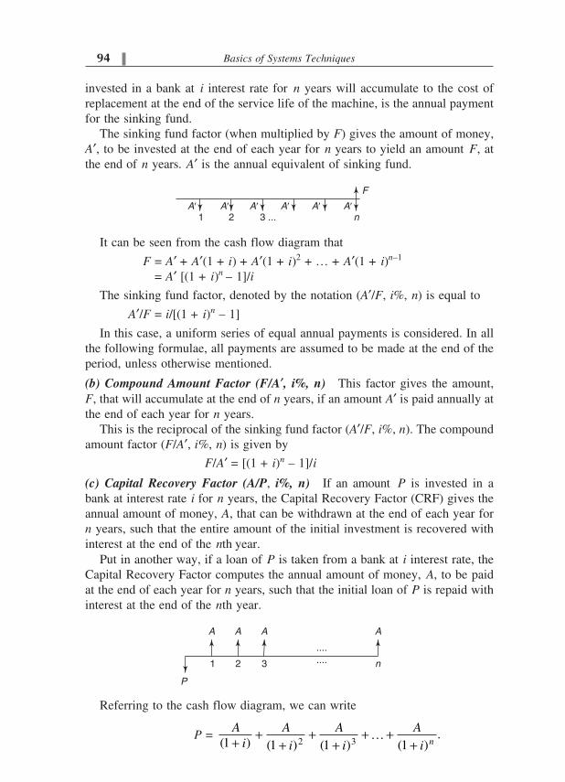
�# Basics of Systems Techniques
invested in a bank at i interest rate for n years will accumulate to the cost of
replacement at the end of the service life of the machine, is the annual payment
for the sinking fund.
The sinking fund factor (when multiplied by F) gives the amount of money,
A�, to be invested at the end of each year for n years to yield an amount F, at
the end of n years. A� is the annual equivalent of sinking fund.
It can be seen from the cash flow diagram that
F = A� + A�(1 + i) + A�(1 + i)2 + … + A�(1 + i)n–1
= A� [(1 + i)n – 1]/i
The sinking fund factor, denoted by the notation (A�/F, i%, n) is equal to
A�/F = i/[(1 + i)n – 1]
In this case, a uniform series of equal annual payments is considered. In all
the following formulae, all payments are assumed to be made at the end of the
period, unless otherwise mentioned.
(b) Compound Amount Factor (F/A�, i%, n) This factor gives the amount,
F, that will accumulate at the end of n years, if an amount A� is paid annually at
the end of each year for n years.
This is the reciprocal of the sinking fund factor (A�/F, i%, n). The compound
amount factor (F/A�, i%, n) is given by
F/A� = [(1 + i)n – 1]/i
(c) Capital Recovery Factor (A/P, i%, n) If an amount P is invested in a
bank at interest rate i for n years, the Capital Recovery Factor (CRF) gives the
annual amount of money, A, that can be withdrawn at the end of each year for
n years, such that the entire amount of the initial investment is recovered with
interest at the end of the nth year.
Put in another way, if a loan of P is taken from a bank at i interest rate, the
Capital Recovery Factor computes the annual amount of money, A, to be paid
at the end of each year for n years, such that the initial loan of P is repaid with
interest at the end of the nth year.
Referring to the cash flow diagram, we can write
P = 2 3
.(1 ) (1 ) (1 ) (1 )n
A A A A
i i i i� � ���
� � � �

Economic Considerations in Water Resources Systems �$
= [(1 ) 1]
.(1 )
n
n
A i
i i
� �
Therefore,
A/P = [i (1 + i)n]/[(1 + i)n – 1]
Note that both A and A� refer to annual values. The notation A is used with
reference to the present amount P, and A� with reference to the future money F,
to express the fact that A and A� are different in value.
(d) Present Worth Factor (P/A, i%, n) This factor gives the present worth of
equal annual payments made at the end of each year for n years if the interest
rate is i.
This is the reciprocal of the Capital Recovery Factor and is equal to
P/A = [(1 + i)n – 1]/[i (1 + i)n]
It may be noted that the Capital Recovery Factor, (A/P, i%, n), accounts for
both the interest and the sinking fund due to depreciation and is equal to the
sum of the interest rate and the sinking fund factor, as
(A/P, i%, n) = [i (1 + i)n]/[(1 + i)n – 1]
= [i {(1 + i)n – 1} + i ]/[(1 + i)n – 1]
= i + i/[(1 + i)n – 1]
= interest rate, i + sinking fund factor, (A�/F)
This means that the capital recovery is equal to the interest plus depreciation
on an annual basis. The equivalence may be seen from the following example.
Note: As n �, A/P , i, meaning that over a large repayment period, the
capital recovery boils down to the interest with negligible amount to be raised
as the sinking fund.
Lt (A/P, i%, n) = i
n �If A is the constant annual payment to be made on a perpetual basis, the
equivalent present cost indicated by the value, A/i, is termed as the capitalized
cost.
In the examples illustrated in this section, the numerical values of the dis-
count factors, where necessary, were directly used as obtained from the appro-
priate expressions, for the required values of the interest rate, i, and the number
of years, n.
������������ Suppose we buy a pump for Rs 10,000 today. It has a service
life of 10 years with no salvage value at the end of its service life. We take a
loan of Rs 10,000 from the bank at 6% interest rate.
The amount required to be paid at the end of each year to the bank to repay
the loan completely in 10 years with interest is
A = 10,000 � Capital Recovery Factor, [A/P, 6%, 10], with i = 6 and n = 10.
= 10,000 � 0.13587 = Rs 1,358.7

�% Basics of Systems Techniques
The loan of Rs 10,000 will be repaid with interest if Rs 1,358.7 is paid to
the bank at the end of each year for 10 years.
On the other hand, we bought the pump for Rs 10,000 (borrowed from the
bank) and it is in our hands today (but we have no other money). Every year,
we raise a fund and, at the end of the year, deposit in the bank to have enough
money at the end of 10 years to buy another new pump. Assuming that the
cost of the pump remains the same, and that money grows at the same interest
rate i (as when we borrowed the money to buy the pump), the annual sinking
fund is
A� = 10,000 � sinking fund factor [A�/F, 6%, 10] with i = 6 and n = 10
= 10,000 � 0.07587 = Rs 758.7 (This is the monetary equivalent of the
annual depreciation of the pump).
With this annual payment, we will have Rs 10,000 at the end of 10 years in
the bank to buy a new pump. Only then, at the end of 10 years we will be in
the same position as we are now. But remember, we should also pay the bank
interest annually on the borrowed money of Rs 10,000 at 6% per year. This
annual interest amount is
Annual interest = Pi
= 10,000 � .06 = Rs 600
which is the exact difference between the amounts A and A�,(A – A� = 600),
i.e. Amount of capital recovery = Interest + Sinking fund (annual)
����� �� �"�&�"� �
Amortization is the term generally used to indicate payment of a debt in equal
instalments at uniform intervals of time. Part of each payment is credited as
interest and the remaining towards repayment of loan. For example, if we
borrow Rs 100,000 from the bank to be repaid in 10 years at 6 per cent interest
rate, then the equal instalment of money to be paid at the end of each year is
A = Annual instalment = Principal amount � Capital recovery factor
= P (A/P, i%, n) = 100,000 � (A/P, 6%, 10) = 100,000 (0.13587) = 13,587
This is the exact amount to be paid at the end of each year. For any given
year, this has two components, one is the interest on the outstanding balance of
the loan at the beginning of the year and the other is the amount credited
towards repayment of the loan itself.
Each year, though we pay to the bank the same amount of Rs 13,587
annually, the amount credited towards interest and towards debt reduction
(repayment) will be different in different years, because the interest in a year is
computed based on the outstanding balance (of debt) at the beginning of the
year. For example, for the first year, the interest component will be 6% of
100,000, which is 6,000. At the end of first year, then, out of Rs 13,587 paid to
the bank, the bank would credit Rs 6,000 as interest, and the remaining amount
of Rs 7,587 (= Rs 13,587 – Rs 6,000) towards repayment of the loan. Thus the
outstanding loan at the beginning of the second year is Rs 100,000 – Rs 7,587
= Rs 92,413, and so on.

Economic Considerations in Water Resources Systems �'
We can determine the components of interest and repayment (of loan) out of
the equal annual instalment paid, at the end of any year, x, as follows:
We first find out the repayment component in the year x.
�������
Repayment is made by building a sinking fund through equal annual payments,
A�, at the end of each year. The total fund in n years at i% interest rate should
accumulate to P, when an amount A� is deposited in the bank at the end of each
year for n years.
Thus A� = (Principal borrowed) � (Sinking fund factor) = P (A�/F, i%, n)
The total amount paid towards debt or loan at any point of time is equal in
value to the sinking fund raised till that point of time.
The total amount paid towards repaying the loan till the end of year x
Dx = A� + A� (1 + i) + A� (1 + i)2 + … +A� (1 + i)x–1
= A� [(1 + i)x – 1]/i
Similarly, the total amount paid towards repaying the loan till the end of year
x – 1 is
Dx – 1 = A� [(1 + i)x – 1 – 1]/i
Therefore, the amount paid towards repayment of loan in the year x,
�Dx = Dx – Dx–1 = A� {[(1 + i)x – 1]/i – A� [(1 + i)x–1 – 1]/i}
= A� (1 + i)x–1
We know that A�, the annual sinking fund, is equal to
A��= P (A�/F, i%, n) = P {i/[(1 + i)n – 1]}
Therefore, �Dx = Pi(1 + i)x–1/[(1 + i)n – 1],
which is the repayment component in the year x. Since A = Interest + Repay-
ment, the interest component for year x = A – �Dx.
������� ����� For the problem mentioned earlier, where P = 100,000,
i = 6% and n = 10 yrs, the yearly components of repayment and interest are
shown in the following table.
P = 100,000; i = 6%, n = 10 yrs
A = 13,586.80 A� = 7,586.80
Year Repayment, �Dx Balance Interest
col 1 col 2 col 3 col 4
1 7,586.80 92,413.20 6,000.00
2 8,042.00 84,371.20 5,544.79
3 8,524.52 75,846.68 5,062.27
4 9,036.00 66,810.68 4,550.80
(Contd.)

�( Basics of Systems Techniques
(Contd.)
P = 100,000; i = 6%, n = 10 yrs
A = 13,586.80 A� = 7,586.80
Year Repayment, �Dx Balance Interest
col 1 col 2 col 3 col 4
5 9,578.15 57,232.53 4,008.64
6 10,152.84 47,079.68 3,433.95
7 10,762.01 36,317.67 2,824.78
8 11,407.74 24,909.93 2,179.06
9 12,092.20 12,817.73 1,494.60
10 12,817.73 0 769.06
col 1 : year number,
col 2 : repayment in the year, �Dx (end of year value),
col 3 : outstanding balance of loan at the beginning of the year in col 1
= P – Dx,
col 4 : Interest for the year credited at the end of the year = A – �Dx
Note that the interest component will be relatively high and the repayment
low in the initial years, while the trend reverses in the latter years.
�����������# A person borrows a sum of Rs 50,000 @ 6 per cent interest
for 10 years. Determine the equal annual sum to be paid at the end of each
year to repay the loan, and the amounts credited towards interest and repay-
ment in the 5th year.
1. The amount of money to be paid at the end of each year
= 50,000 [P/A, 6%, 10] = 50,000 (.1359) = 6795
2. Year x = 5 ; A = 6795
Annual sum paid at the end of 5th year, A = Rs 6795
The sinking fund, A� = 50,000 (A�/F, 6%, 10)
= 50,000 (.0759) = 3795
The repayment component (reduction in the principal borrowed)
in the 5th year = A� (1 + i)x–1
Payment, �Dx = 3795(1 + 0.06)4 = 4791
� Interest component = A – �Dx
= 6795= 4791 = 2004
� At the end of 5th year,
interest component = Rs 2004
repayment component = Rs 4791
out of the annual amount of Rs 6795 paid
Annual Costs The annual cost (AC) of a project consists of the following:
1. Interest on the borrowed capital
2. Depreciation or amortization cost
3. Operation and maintenance cost (O&M cost), and
4. Other costs, specified, if any
The first two costs sum up to the capital recovery on an annual basis.

Economic Considerations in Water Resources Systems ��
����# � ������ � )��"����"�*������
The background information dealt with so far will be useful in the economic
evaluation of alternative proposals for specified needs. The comparison may be
based on any of several available methods, but a proper economic evaluation
(based on any method) should result in an identical selection. Two of the most
common methods used are illustrated in the following pages: present worth
method and the equivalent annual cost method. The use of these two methods
is illustrated next with examples.
Note that the present worth is a function of the duration of analysis and,
therefore, any comparison of alternatives should be based on the same period
of analysis for each alternative. In this respect, comparison on the basis of
equivalent annual cost is relatively easier.
������� ����$ Which of the following plans is more economical at 6%
interest rate?
Plan A Plan B
Cost of Equipment 50,000 35,000
Annual O & M Costs 2,000 2,500
Salvage value 7,000 6,000
Service life 30 years 15 years
Let us compare the two alternate plans by different methods
1. Equivalent Annual Cost (AC)
Plan A
Annual Cost = Interest + Depreciation + O & M costs
Interest on borrowed capital = 50,000 � .06 = 3000
Depreciation = (P – L) (A�/F, 6%, 30)
= (50,000 – 7,000) (.01265) = 543.95
O & M Costs = 2000
Total AC = 3000 + 543.95 + 2000 = 5543.95
Plan B
Interest = 35,000 � .06 = 2100
Depreciation = (35,000 – 6,000) , 6%,15A
F
�� �� �� �
= 29,000 � (0.04296)
= 1245.84
O & M Cost = 2500
Total AC = 2100 + 1245.84 + 2500
= 5845.84
Plan A is preferable because of lower annual cost.
2. Present Worth (PW) Comparison
As mentioned earlier, PW should be compared for equal periods of
analysis in both plans. Let us compare the plans on a 30-year basis. For
this purpose, the life of plan B is extended by another 15 years with

�++ Basics of Systems Techniques
identical expenditure pattern as in the first 15 years. A comparison of
present worth of all costs can be made then, based on an analysis period
of 30 years.
Plan A (30 years)
PW of initial cost 50,000 = Rs 50,000
PW of salvage value = –7000 (P/F, 6%, 30)
(negative cost) = –7000 (0.17411) = –1218.77
PW of O & M Costs = 2000 (P/A, 6%, 30)
= 2000 (13.7648) = 27,529.60
PW of total cost = 50,000 – 1218.77 + 27,529.60
= 76,310.83
Plan B (for 30 years)
PW of initial cost of 35,000 = 35,000
PW of 35,000 at 15 years = 35,000 (P/F, 6%, 15)
= 35,000 (.41727) = 14604.45
PW of 6000 (negative cost at 15 years)
= – 6000 (P/F, 6%, 15)
= – 6000 (.41727) = –2503.62
PW of 6000 (negative cost at 30 years)
= – 6000 (P/F, 6%, 30)
= – 6000(.17411) = –1044.66
PW of O & M Costs = 2500 (P/A, 6%, 30)
= 2500 (13.7648) = 34,412
PW of Total Costs
= 35,000 + 14,604.45 – 2503.62 – 1044.66 + 34,412
= 80467.72
Because of lower costs Plan A is preferred to Plan B.
Note: The annual costs worked out in method 1 may be obtained from the
present worth calculated above by applying the capital recovery factor, (A/P,
6%, 30) = 0.07265
AC of Plan A = (PW)A .(A/P, 6%, 30)
= (76,310.83) (.07265) = 5543.98
AC of Plan B = (PW)B . (A/P, 6%, 30)
= (80,465.72) (.07265) = 5845.98
which are same as before except for rounding off of errors.
������� ����% There are two alternatives to water supply in an irrigation
district. Plan A is to construct an open channel at an initial cost of
Rs 50,00,000 with O & M cost of Rs 400,000 per year. The alternative, Plan
B, is to go for a piping system at an initial cost of Rs 90,00,000 and an O &

Economic Considerations in Water Resources Systems �+�
M cost of Rs 50,000/year. Money is available for 6% interest rate, and sinking
fund will improve at 4% interest. Useful life of the project in both cases is 20
years. Select the more economical of the two alternatives.
Let us work out the annual costs in both cases.
Plan A Plan B
Interest at 6% 300,000 540,000
Depreciation @ 4% 167,500 301,500
(A�/F, 4%, 20)=.0335 on P
O & M Costs 400,000 50,000
Total 867,500 891,000
� Plan A is preferable to Plan B.
Note: In this example, the interest rate on borrowed money and the discount
rate for depreciation are different.
Problems
3.1.1 A bank gave 10 per cent interest, compounded every two months for
the first six months of a year. Subsequently, the bank decided to give
only 8 per cent interest, compounded monthly, for the rest of the year.
What was the effective rate of interest for that year?
(Ans: 9.36%)
3.1.2 An equipment costs Rs 800,000 today and has a service life of 15
years. If the salvage value at the end of 15 years is Rs. 200,000,
determine its appraisal value at the end of 10 years. Interest rate
= 10%. (Ans: Rs 499,070)
3.1.3 A person takes a loan from a bank: Rs 5000 now, Rs 2000 at the end
of 2 years, Rs 3000 at the beginning of the 5th year, and equal amounts
of Rs 1000 each beginning 6th year for 10 years. Determine what
equal annual instalments (end of year) he should pay for 15 years in
order to repay the loan with interest at 10 per cent.
(Ans: Rs 1696.19)
3.1.4 A pipeline is proposed to be laid from an existing pumping station to a
nearby reservoir. Two alternate possible pipe sizes are considered:
Pipe size Cost/hr of pumping (Rs) First cost of construction (Rs)
A 5.0 80,000
B 3.0 160,000
Both pipe sizes have a life of 15 years, with no salvage value. Interest
rate is 6%.
(i) Which is the most economical pipe size, if the total number of
hours of pumping per year is 5000. Compare equivalent annual
costs.
(ii) How many hours of pumping per year are required to make the
two pipe sizes equally economical.
(Ans: (i) pipe size A (ii) 4120 hrs/yr)

�+� Basics of Systems Techniques
��� �� ���� �,-���
A discussion of the market supply and demand is necessary before we go into
the benefit cost analysis of project planning.
Types of Goods in the Market In general, goods can be classified into two
categories:
1. Normal goods, or personal goods, or private goods, and
2. Collective goods, or public goods.
Normal goods have the property of being consumed by individuals, such
that, given a fixed quantity, more units for one means fewer for others and vice
versa. Most of the goods for which a real market exists come under this
category. For example, for a fixed number of automobiles produced, the more
one section of the people buy them, the less they are available for others (to
buy), and vice versa. However, there are some other goods for which this is not
true. National defence and flood control are examples of these. Here each one
“consumes” the same amount of national defence, and, although each person
added to the population consumes national defence, his/her consumption does
not necessarily make it less available for the rest of the population. These
goods are called collective goods, or public goods, in contrast to the normal,
or personal or private goods.
����� ���.�"�����/��/�!���0
Demand is the quantity per unit time that people will be willing to buy, ex-
pressed as a function of the price, all other factors remaining constant. The
demand curve has the property that it slopes downward to the right because
lower prices increase sales (more number of buyers), and higher prices de-
crease them (less number of buyers).
�����������������������
Let us consider a demand curve, Fig. 3.1, which depicts a linear relation be-
tween price and the quantity demanded.
��1���� ����������� ����������
A demand curve indicates the change in the demand or sales for a given
change in the price. This relationship is given by the price elasticity of demand,

Economic Considerations in Water Resources Systems �+�
E, which is defined as the ratio of the relative change in the quantity, for a
given relative change in the price. If Q is the demand at price P, then the price
elasticity of demand E is given by
E = – (�Q/Q) � (�P/P) = – (�Q/�P)(P/Q) (12.1)
The negative sign indicates that Q increases as P decreases (slope of the
demand curve is negative). In the case of the linear demand curve shown in
Fig. 3.1, though the slope remains constant at all points on it, the elasticity of
demand changes from point to point on the curve. It varies from infinity along
the vertical axis (E = �) to zero along the horizontal axis (E = 0).
A value for E of infinity (point A on the linear demand curve) indicates a
perfectly elastic product, which no one will buy if the price is raised. At this
price, goods become perfectly elastic and are completely priced out of the
market. A value for E of zero (point B on the linear demand curve) indicates a
perfectly inelastic product, i.e. one for which the price has no effect on demand.
In between these two extremes, a given product may be elastic or inelastic at a
given price, depending on its relation to the demand as defined by the demand
curve, in other words, on the price elasticity of demand, E.
As the price is reduced from point A, elasticity decreases, until it reaches
unity at some point C, when the product is no longer said to be elastic. For all
points on the line above C, the price elasticity of demand, or simply the elastic-
ity as it is often called, is E > 1. The total revenue, which is the product of the
price and the quantity of goods sold (P.Q) increases up to this point, as the
increase in sales (demand) offsets the reduction in price resulting in an increase
in the gross revenue. The point C (point of unit elasticity, E = 1) provides the
supplier the largest revenue. If the price is reduced further down the point C,
though demand continues to increase, the increase will not be fast enough to
offset the decreasing price resulting in a decline in the gross revenue from that
at point C. For all points below C, the price elasticity will be less than unity,
(E < 1). In this region, the product is said to be inelastic. It is to be noted that
the same product is inelastic at low prices and elastic at high prices.
�����������
The supply curve shows the relationship between the quantity produced and the
price at which the producers are willing to sell, other things remaining
constant. Typically, a supply curve slopes upward to the right, meaning that
more goods will be produced, and more sellers will enter the market as the
price increases.
������������������������
A market consists of sellers and buyers. The behavior of each group is, how-
ever, different. The buyers’ behavior is reflected by the demand curve and that
of the sellers by the supply curve. The buyers would like to minimize the
expenditure and the sellers would like to maximize their revenue from sales.

�+# Basics of Systems Techniques
The demand curve and the supply curve therefore combine to establish the
equilibrium market price. The equilibrium price is the minimum under conditions
of pure competition that each individual buyer must pay per unit quantity
purchased and the maximum that each seller can receive for each unit quantity
sold (James and Lee, 1971).
That this equilibrium point corresponds to a point of unit elasticity on the
demand curve can be shown as follows:
The total revenue from sales or the total expenditure, G, for goods pur-
chased is given by
G = price � quantity = P � Q
For this to be optimum, dG/dP = 0
dG/dP = P dQ/dP + Q = 0
or dQ/dP = – Q/P
or – (P/Q) � dQ/dP = E = 1
The left-hand side is the price elasticity of demand by definition. Therefore,
the market equilibrium prevails at the price corresponding to E = 1 on the
demand curve. This analysis presumes that free market conditions exist with no
restrictions and there is free entry for an unlimited number of buyers and
sellers. At this equilibrium price, the sellers would have maximized their re-
turns and the buyers would have minimized their total expenditure.
We will not discuss in this book the consequences of a shift in demand or
the effect of subsidies on market behavior.
����� �11��1�"� � )�����/
The procedure for aggregating demand curves depends on the type of product.
In the case of a normal product (market good), where consumption is mutually
exclusive (what is consumed by one is not available to the others—e.g. drink-
ing water), the combined demand curve is generated by adding the demands of
each individual at a given price. Thus, the combined demand is computed at
each price and plotted to get the aggregate demand curve. This horizontal
addition of demands is characteristic of normal or market goods.
In the case of a collective good, however, where the consumption is not
mutually exclusive (example—flood control), the prices are added up for a
given demand and for all demand levels. This type of vertical addition of price
is characteristic of collective or public goods.
Figures 3.2 and 3.3 show examples of how this aggregation is done graphi-
cally for normal goods (such as irrigation water) and for collective goods (such
as flood control), respectively.
The aggregate demand curves can be arrived at analytically as well, if the
equations of individual demand curves are given.

Economic Considerations in Water Resources Systems �+$
������������ Water is supplied from a project for two types of uses: rural
and urban. The demand curve for rural use is given by P + 3y = 30, and the
demand curve for urban use is 4P + y = 40, where y is the demand and P is
price in appropriate units. Determine the combined demand curve.
Graphical Method
The rural and urban demand curves are first plotted individually. The com-
bined demand curve is obtained by adding the individual demands at a given
price as, in this case, water is a normal good.
��1���� ��������� ���������������������������
��1���� ��������� �����������������������������

�+% Basics of Systems Techniques
Analytical method
Let rural demand = yr at price P
urban demand = yu at price P
y = yr + yu at the same price P for a normal good.
yr = (30 – P)/3
yu = 40 – 4P
For P � 10 (or y � 20/3),
y = yr + yu = (30 – P)/3 + 40 – 4P = 50 – (13/3)P, or 13P + 3y = 150,
where y is the combined demand.
For P � 10, (or y � 20/3),
y = yr = (30 – P)/3 or P + 3y = 30
Combined demand curve is given by
P + 3y = 30 for P � 10
and 13P + 3y = 150 for P � 10.
������������ Two different groups of people are affected by a flood con-
trol project. The demand for flood control from the two groups are as follows:
Group 1 P + 3y = 30
Group 2 4P + y = 40
where P is price and y is the level of protection provided.
Determine the aggregate demand curve.
Graphical Method In this case, the ‘consumption’ is not mutually exclusive
as flood control is a ‘collective good’. Therefore, the combined demand is
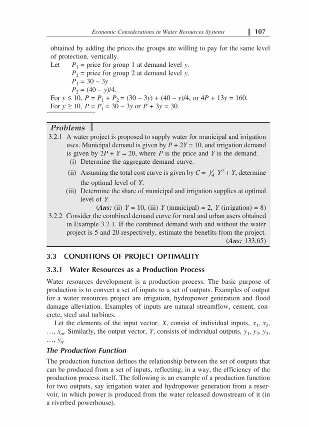
Economic Considerations in Water Resources Systems �+'
obtained by adding the prices the groups are willing to pay for the same level
of protection, vertically.
Let P1 = price for group 1 at demand level y.
P2 = price for group 2 at demand level y.
P1 = 30 – 3y
P2 = (40 – y)/4.
For y � 10, P = P1 + P2 = (30 – 3y) + (40 – y)/4, or 4P + 13y = 160.
For y � 10, P = P1 = 30 – 3y or P + 3y = 30.
Problems
3.2.1 A water project is proposed to supply water for municipal and irrigation
uses. Municipal demand is given by P + 2Y = 10, and irrigation demand
is given by 2P + Y = 20, where P is the price and Y is the demand.
(i) Determine the aggregate demand curve.
(ii) Assuming the total cost curve is given by C = 14 Y 2 + Y, determine
the optimal level of Y.
(iii) Determine the share of municipal and irrigation supplies at optimal
level of Y.
(Ans: (ii) Y = 10, (iii) Y (municipal) = 2, Y (irrigation) = 8)
3.2.2 Consider the combined demand curve for rural and urban users obtained
in Example 3.2.1. If the combined demand with and without the water
project is 5 and 20 respectively, estimate the benefits from the project.
(Ans: 133.65)
��� � ��2� ����3��2�2���,�2-
����� 4�"����� !��������� /!�"� ��� ����
Water resources development is a production process. The basic purpose of
production is to convert a set of inputs to a set of outputs. Examples of output
for a water resources project are irrigation, hydropower generation and flood
damage alleviation. Examples of inputs are natural streamflow, cement, con-
crete, steel and turbines.
Let the elements of the input vector, X, consist of individual inputs, x1, x2,
…, xm. Similarly, the output vector, Y, consists of individual outputs, y1, y2, y3,
…, yn.
!������������� �������
The production function defines the relationship between the set of outputs that
can be produced from a set of inputs, reflecting, in a way, the efficiency of the
production process itself. The following is an example of a production function
for two outputs, say irrigation water and hydropower generation from a reser-
voir, in which power is produced from the water released downstream of it (in
a riverbed powerhouse).

�+( Basics of Systems Techniques
The region below the curve containing the origin is the technologically
feasible region. Any combination of outputs above the curve (on the side of the
curve away from the origin) is infeasible. A combination of outputs repre-
sented by points within the feasible region will be inefficient. For example, for
a given amount of irrigation water supply, y1, there is a maximum of hydro-
power, y2, that can be produced from the reservoir, represented by the point A
on the curve. Anything below A is feasible, but inefficient, and anything above
A is infeasible. Thus A represents the maximum possible y2 corresponding to
y1. Thus, the curve represents the locus of efficient points in the production
process. This is also called the efficiency frontier curve or production possibil-
ity frontier. The production function is a mathematical representation of this
line. It is related to the input and output vectors and, putting all the terms on
the left-hand side, it is expressed as
f (X, Y ) = 0 (3.1)
While every point on the production function represents an efficient point
(efficient operation of the system), the selection of the best point, however,
requires value judgment. Each point on the production function (also termed a
pareto-admissible solution) represents a relative value associated with each
variable. The objective function is a function of both the input and the output
vectors. The net benefit objective function, u = u (X, Y ), is expressed as
u = i i j ji j
b y c x� � (3.2)
where bi refers to the unit benefit associated with the ith output element, and cj
refers to the unit cost associated with the jth input element.
"#$������� �������
The objective is to maximize net benefits such that the solution point lies on
the production frontier line, i.e. to maximize the objective function, u = u(X,
Y), subject to the constraint, f(X, Y) = 0, where X and Y are input and output
vectors containing m and n elements, respectively.
The Lagrangean formed from the objective and the constraint is written as
L = u(X, Y ) – � f (X, Y) (3.3)
��1���# ������������������������������

Economic Considerations in Water Resources Systems �+�
where � is the Lagrangean multiplier and L is the function to be maximized.
The necessary conditions for optimality are obtained by differentiating L par-
tially with respect to each xi, each yj and �, and setting each partial differential
to zero. Thus, there will be m + n + 1 equations with m + n + 1 unknowns (m
inputs, n outputs, and �). Solving this set of simultaneous equations results in
the optimal levels of inputs and outputs.
�u(X, Y )/�xi = ��f (X, Y )/� xi for i = 1, 2, …, m (3.4)
�u(X, Y )/�yj = �� f (X, Y )/� yj for j = 1, 2, …, n (3.5)
�u(X, Y )/�� = f (X, Y )
Setting this last equation to zero means that the constraint, Eq. (3.1) must be
satisfied.
By dividing Eq. (3.4) for two inputs x1 and x2, Eq. (3.5) for two outputs y1
and y2, and pairs of equations for one input, xi, and one output, yj, one obtains
the following equations:
[�u(X, Y )/�x1]/[�u(X, Y)/�x2 ] = [� f(X, Y)/�x1 ]/[� f(X, Y)/�x2] (3.6)
[�u(X, Y )/�y1]/[�u(X, Y)/�y2 ] = [� f(X, Y)/�y1 ]/[� f(X, Y)/�y2] (3.7)
[�u(X, Y )/�xi]/[�u(X, Y)/�yj ] = [� f(X, Y)/�xi ]/[� f(X, Y )/�yj] (3.8)
Since f (X, Y) must equal zero, an increase in one element must be offset by
a decrease in another. Thus:
[� f(X, Y )/�x1]/[� f(X, Y )/�x2] = –[�x2/�x1] (3.9)
[� f(X, Y )/�y1]/[� f(X, Y )/�y2] = –[�y2/�y1] (3.10)
[� f(X, Y )/�xi]/[�f (X, Y )/�yj] = –[�yj/�xi] (3.11)
Combining Eqs (3.6) and (3.9), (3.7) and (3.10), and (3.8) and (3.11), one
finally gets
[�u(X, Y )/�x1]/[�u(X, Y )/�x2 ] = –[�x2/�x1] (3.12)
[�u(X, Y )/�y1]/[�u(X, Y )/�y2 ] = –[�y2/�y1] (3.13)
[�u(X, Y )/�xi]/[�u(X, Y )/�yj ] = –[�yj/�xi] (3.14)
����� � �/�"� �� )�"�����"0
The following can be interpreted easily.
�u(X, Y )/�xi = rate of change of the net benefit function with respect
to input i, or the marginal cost of input xi = MCi
�u(X, Y )/�yj = rate of change of benefit function with respect to output
j, or the marginal benefit of output yj = MBj
It is to be emphasized that, whenever the change of one element with respect
to another is considered, all other elements are held at constant levels.
The right-hand side of Eq. (3.12) is termed as the marginal rate of
substitution, MRS21, which is defined as the marginal rate at which the second
input needs to be substituted for the first input, holding the level of production
constant. Thus, Eq. (3.12) gives
MC1/MC2 = MRS21 (3.15)

��+ Basics of Systems Techniques
The right-hand side of Eq. (3.13) is termed as the marginal rate of transfor-
mation, MRT21, Thus Eq. (3.13) gives
MB1 /MB2 = MRT21 (3.16)
The right-hand side of Eq (3.14) is termed as the marginal physical produc-
tivity of the ith input when devoted to the jth output, or the marginal physical
product, MPPij Thus Eq. (3.14) gives
MCi /MBj = MPPij (3.17)
Equations (3.15), (3.16), and (3.17) are the three conditions of optimality
that are necessary to achieve maximum net benefit.
Note: It must be noted that the conditions of optimality are necessary but not
sufficient conditions. Sufficiency requires that there be no higher value of the
objective function than is indicated by the solution. Even then, the solution can
only be a local maximum and need not be a global maximum. For a more
practical interpretation of those theoretically derived expressions, see Maass et
al. (1968) and James and Lee (1971).
������������ Combination of Inputs (Marginal Rate of Substitution)
A water resources project has the option of using two inputs, reservoir water
and groundwater, to provide irrigation to a given area. All other things being
equal, the need is satisfied by the combination of inputs, x1 and x2, as shown
in Fig. 3.5. To determine the best combination of these inputs, the first
optimality condition says that the levels of x1 and x2 should be in the ratio of
MC2 to MC1.
0
10
20
30
40
50
60
70
80
90
0 100 200 300 400
x x1 2= 50; = 45 (opt)
x1
x2
��1���$ �������������� �����
MC1 = 10; MC2 = 4; (MRS21)opt = MC1/MC2 = 2.5
Sl No. x1 x2 |�x1| |�x2| MRS21 Total cost
1 80 10 840
2 65 25 15 15 1 750
3 55 40 10 15 1.5 710
4 45 65 10 25 2.5 710
5 20 190 25 125 5 960
6 5 340 15 150 10 1410

Economic Considerations in Water Resources Systems ���
For the data shown in the table, the optimal marginal rate of substitution
is MC1/MC2 = 2.5. This would correspond to x1 = 50 and x2 = 45, as shown
in the figure. At this point, it is seen that a line with a slope of
2 1
1 2
2.5x MC
x MC
�
�
� �� �� �� � is tangential to the curve as desired. The total cost would
be a minimum (= 680, in the present example) at this point.
������������ Combination of Inputs (Marginal Rate of Substitution)
Two inputs x1 and x2 should be combined to satisfy the relationship x1x2 = 16,
in order to produce constant results (output), all other things being the same.
x1 and x2, for example, may represent the quantum of surface water and
groundwater to provide a given level of irrigation to a given area. If the
marginal costs of x1 and x2 are 4 and 1, respectively, determine the optimum
values of x1 and x2.
The desired point (x1, x2) should lie on the curve x1x2 = 16. From the first
condition of optimality for two inputs,
2
1
x
x
�
� = MRS21 = 1
2
4
1
MC
MC� = 4
where x1x2 = 16; 21 2
1
xx x
x
�
�� = 0 or 2 2
1 1
x x
x x
�
��
2
1
x
x
�
� = 2 1
1 2
x MC
x MC� = 4 � x2 = 4x1
As (x1, x2) should lie on the curve, x1 (4x1) = 16
or 214x = 16
� x1 = 2
and x2 = 4x1 = 8
The minimum cost at this level of input combination = x1 (MC1) + x2 (MC2)
= 2(4) + 8(1) = 16
Alternate Method
C = Total cost of production = x1(MC1) + x2(MC2)
= 4x1 + 1x2
For C to be a minimum, 1
C
x
��
= 0, or 2
1
4 0x
x
�
�� �
or 2
1
4x
x
�
��
The minimum point also lies on the curve x1x2 = 16, which by differentiation
gives
21 2
1
dxx x
dx� = 0 or 2 2
1 1
x x
x x
�
��

��� Basics of Systems Techniques
� 2
1
x
x
�
�= 2
1
4x
x �
� x2 = 4x1
As x1x2 = 16, x1 = 2 and x2 = 8, as before.
Note: The results are the same in both methods as both tend to maximize the
objective of net benefits. But in this case, since the benefits are constant,
optimization boils down to minimizing the cost.
������������ Combination of Outputs (Marginal Rate of Transformation)
Two outputs can be produced from a production process such that the levels
of the two outputs, y1 and y2, satisfy the relation, 2 21 24y y� = 4, keeping all
other things constant. If the marginal benefits of y1 and y2, are respectively
equal to 10 and 5, determine the optimum levels of y1 and y2.
y1 and y2 can denote, for example, irrigated area and hydropower generated
respectively. It is assumed that the water used for these two is mutually
exclusive. What is used for one is not available for the other. This can result
if water is withdrawn from reservoir storage for diversion into canals for
irrigation, and hydropower is produced only from the water released
downstream of the reservoir.
Optimum value of y1 and y2 should lie on the curve (production function)
2 21 24y y� = 4
Diff. with respect to y1, 2y1 + 22
1
8y
yy
�
�= 0
or 2
1
y
y
�
�= 1
2
1
4
y
y
From the second condition of optimality,
2
1
y
y
�
� = MRT21 = 1
2
MB
MB; and MB1 = 10, MB2 = 5
� 1
2
1
4
y
y� � =
10
5 = 2, or y1 = 8y2
As 2 21 24y y� = 4, 2 2
2 264 4y y� = 4 or y2 = 1/ 17 and y1 = 8/ 17
The benefit at this level will be maximum = y1(MB1) + y2 (MB2 )
= 8/ 17 (10) + 1/ 17 (5)
= 85/ 17
Alternatively, the problem may be solved directly using the Lagrangean
multiplier method.
Maximize u = 10y1 + 5y2

Economic Considerations in Water Resources Systems ���
subject to 2 21 24y y� = 4
Necessary Condition:
Lagrangean L = 10y1 + 5y2 – � ( 2 21 24y y� – 4)
1
L
y
��
= 10 – 2� y1 = 0
2
L
y
��
= 5 – 8� y2 = 0
L���
= – ( 2 21 24y y� – 4) = 0.
Solving y1 = 817
y2 = 117
and B = 8517
[The student may check this for the sufficiency condition.]
������� ����# Combination of an Input and an Output (Marginal
Physical Product, MPP)
Consider a reservoir project operated for irrigation and hydropower in
which the input element is the water supply, x, and the output element is the
hydropower generated, y. Let the marginal cost of water supply be MCx = �,
and the marginal benefit of hydropower generation is MBy = �, where � and �
are constants. Let x and y be related as y = x within the feasible ranges of x
and y. The question is how much of x should be used to produce y under
optimal conditions, all other quantities being the same. The rule says:
y
x
�
� = MPPxy = x
y
MC
MB
i.e., increase the value of x until the point where the ratio of marginal output
to marginal input equals the marginal physical product, which is the ratio of
the marginal input cost to the marginal output benefit.
Note: the marginal cost, as determined by partial differentiation of the net
benefits, (� y –�� x), is –�.
When y x = 0, 1
2
y
x x
�
� � = ;
��
x = 1
4(� /�)2
For maximum net benefits, x = 1/4(� /�)2 and y = 1
2(� /�)
Alternatively, using the Lagrangean Multiplier method directly,

��# Basics of Systems Techniques
Maximize u = �y – �x
subject to y – x = 0.
L = � y – � x– � (y – x )
L
x
��
= –� + 2 x
� = 0.
L
y
��
= � �– ��= 0
L���
= – (y – x ) = 0
Solving x = 1
4(� /� )2, y =
1
2(� /� )
This is a necessary condition for local maximum.
[The student may check this for the sufficiency condition.]
Problems
3.3.1 Water from two different sources is supplied to satisfy the industrial
needs of a power plant. Let x1 = supply from source 1 at a cost of
� /unit-volume, and x2 = supply from source 2 at a cost of � /unit-
volume. Any combination of x1 and x2 such that x1x2 = k2, where k is a
constant, would satisfy the industrial requirement. Determine the optimal
values of x1 and x2 (for total cost minimization).
3.3.2 The area that can be irrigated, x, and the hydropower that can be
generated, y, from a given reservoir are related by the first quadrant of
an ellipse, a curve 22
2
2 2
yxC
a b� � , each combination resulting in the
best utilization of all inputs, where a, b, and c are constants. Determine
the optimal levels of x and y, if the marginal benefits of x and y are �and �, respectively.��Note: For a given x, no more of y than is determined by the equation
222
2 2
yxC
a b� � is possible, and vice versa. That is, the optimum (x, y)
should lie on this curve and the slope of the tangent at this point
should be (� /�). ��
��# �� ���2��2� �,-���
The primary purpose of a water resources project is its utility to the public.
Obviously, a given project will not be beneficial to everyone who may be
affected by it. Some will be positively benefited and some negatively. Benefi-

Economic Considerations in Water Resources Systems ��$
ciaries can be individuals, communities, groups of people, or entities such as
administrative districts. For example, a reservoir may benefit all those down-
stream by providing the benefits of irrigation, low-flow augmentation, hydro-
power generation, flood-damage alleviation etc; whereas, those in the upstream
suffer from submergence, inconvenience in rehabilitation and resettlement, etc.
In this context, a plan will be considered economically feasible only if the
positive benefits outweigh the total costs involved in implementing it or, put-
ting it in monetary terms, the benefit cost ratio should be more than one, or the
net benefits (gross benefits minus the total costs) should be positive. It is
important to note that the benefit cost analysis be made with and without the
project rather than before and after. This is because some of the after effects
may occur in course of time, even without the project and therefore cannot be
counted as a justification for the project. Benefit cost analysis provides an
objective assessment of the economic feasibility of each project and provides a
means of selecting the best among those short-listed.
��#�� ����)�"���/� �"�
Benefit cost analysis requires the estimate of both benefits and costs associated
with a plan and should take into account all the parties affected one way or
another by it. Benefits accrue through the use of a commodity or service. The
value of the use, expressed in monetary terms, is the benefit associated with the
plan. There may not exist a market related to the commodity or service and,
therefore, estimation of benefits is not always straightforward and easy. Benefit
cost analysis requires estimation of both benefits and costs in monetary terms.
Benefits are to be estimated by aggregating them to whomsoever they may
accrue from the plan. Cost estimates should ideally reflect opportunity costs
rather than just the market prices for a true comparison. This is rarely done in
practice, however.
��#�� � �"��/����)�"�!�*��
The total cost comprises fixed cost and variable cost. Fixed costs, as the term
indicates, are fixed and do not depend on the level of project output. Variable
costs are marginal costs and vary with level of output. While fixed costs are not
marginal, they do affect the computations of the total benefit cost ratio and the
decision whether the project should be built at all. For example, in a reservoir
sizing problem using LP, if the objective is to minimize the total cost of
reservoir construction (sum of fixed and variable costs, variable costs depend-
ing on the storage), and if the optimal required storage, works out to zero then,
obviously, no reservoir need be built and no costs incurred.
If TC = f(Y) is the total cost at output Y, (Fig. 3.6), for a project of single
output, then the average cost, AC, is given by
AC = TC/ Y = f (Y )/Y
Average cost curves are usually U-shaped. They decrease initially because
of economies of scale, and increase again, as production becomes very large.

��% Basics of Systems Techniques
��1���% !�����������������"�������"����#�����������������
The marginal cost, MC, is given by
MC = df (Y ) /dY = f � (Y )
and is represented by the slope of the total cost curve. The slope represents the
change in total cost with a unit change in the output. Unless the market price
exceeds the marginal cost, no firm would produce an extra unit, and therefore,
the rising limb of the marginal cost curve is a supply curve. It indicates the
price necessary to induce an extra unit of production.
The total cost of production of an output, Y, is the area of the marginal cost
curve to the left of Y. It may be noted that the marginal cost curve intersects the
average cost curve at the latter’s minimum, as
AC = f(Y)/Y is minimum when d{f(Y)/Y}/dY is zero, or
{Y f �(Y ) – f (Y )}/Y 2 = 0
or f �(Y ) = f (Y )/ Y
i.e. MC = AC
Similarly, the marginal benefit is the change in the total benefit per unit of
output. The marginal benefit curve is the demand curve because no buyer will
purchase an extra unit unless it provides him a value that exceeds the cost
incurred. It indicates the maximum price that a firm can afford to spend to
acquire an extra unit. Marginal curves, like average curves, are generally
U-shaped, but justified more to the left (James and Lee, 1971).
��#�� ����)�"��/� �"��"���"� �
As mentioned earlier, benefits and costs need to be estimated in monetary
units. Depending on the ease with which such estimates may be arrived at,
there could possibly be four different situations in relation to the availability of
a market, and its prices representing marginal social values.
1. Market prices exist and reflect true marginal social values, such as in the
case of pure competition (ideal condition).

Economic Considerations in Water Resources Systems ��'
2. Market prices exist but, for various reasons, do not reflect marginal social
values. Example: Subsidized agricultural commodities.
3. Market prices are essentially non-existent, but it is possible to simulate a
market-like process to estimate what users (or consumers) would pay if a
market existed. Example: Outdoor recreation.
4. No real or simulated market-like process is conceivable. Example: Historic
monuments, temples, scenic amenities, etc.
For the first three categories (1, 2, 3) mentioned, benefits and costs can be
measured as the aggregate net willingness to pay of those affected by the
project.
Willingness-to-Pay Criterion The concept of willingness-to-pay is based on
the common experience that a person will not buy a commodity at a cost if, in
his view, the value that he accrues by using the commodity is any less than the
price that he has to pay in acquiring it. In other words, the net benefit that
accrues to him (over and above the cost he pays for it) is what induces him to
purchase the commodity in the market. Assume (Loucks et al., 1981), all
people that are benefited by the plan X are willing to pay B(X) rather than
forego the project. This represents the aggregate value of the project to the
beneficiaries. Let D (X ) equal the amount that all the nonbeneficiaries of plan
X are willing to pay to prevent it from being implemented. The aggregate net
willingness to pay, W (X ), for plan X, is equal to the difference between B (X)
and D (X ), i.e. W (X) = B (X) – D (X).
The rationale implied in the willingness-to-pay criterion is that if B (X) >
D (X), the beneficiaries could compensate the nonbeneficiaries and everyone
would benefit from the project. This, however, has some implications such as
the marginal social value of income to all affected parties is the same. If the
beneficiaries are essentially rich and the nonbeneficiaries are poor, then B (X)
may be larger than D (X) simply because the beneficiaries can afford to pay
more than the nonbeneficiaries.
Market Prices Equal Social Values Let us assume that the price demanded is
p(x), when the quantity available in the market is x (demand curve given). Let
there be an increase in the level of the output from x1 without the project to x2
with the project. Then the willingness-to-pay (which is a proxy for the accrued
benefits) is given by the area under the demand curve for the increased portion
of the output, Fig. 3.7.
��1���' ���������$������������������%��

��( Basics of Systems Techniques
Willingness to pay = 2
1
( )x
x
p x dx� (3.2)
which is the area under the demand curve between x = x1 and x = x2. This is an
estimate of the benefit attributable to the project under contemplation.
������� ��#�� The demand curve for recreation at a reservoir site is
determined as 4P + Y = 30, where Y is the annual demand curve and P is
price in appropriate units. The annual demand was 10 without the reservoir
and is expected to increase to 20 with the construction of the reservoir.
Estimate the benefits of recreation arising from the construction of the reservoir.
The demand curve plots as a straight line, EF, as shown in the following
figure:
Demand Curve for Recreation
The area under the demand curve between y = 10 and y = 20 gives the total
willingness to pay for recreation or, in other words, the benefits due to recre-
ation at the reservoir. The area ACDB = (5.0 + 2.5)/2 � 10 = 37.50. The
benefits are thus estimated to be 37.50.
Market Prices do not Equal Social Values There are several procedures that
can be used depending on the situation. A rather common method is to estimate
the cost of the least expensive alternative and project it as the benefit. However,
the alternative cost approach is meaningless in the absence of proof that the
second best alternative would be built if the best were not. As an example, let
the benefits from generating hydroelectricity be estimated using this approach.
Let the alternatives considered be geothermal or nuclear sources. both of which,
let us assume, are more expensive than the hydroelectric scheme. Then the cost
of the least expensive alternative of the two sources will be higher than the cost
of the proposed hydroelectric scheme itself, and hence the proposal will have a
benefit cost ratio higher than one. However, this approach to benefit estimation
is valid only when there is a commitment to actually build the less expensive of
the geothermal and the nuclear schemes, in case the hydroelectric scheme is
not built. Therefore, this method is rather tricky in that it is possible to propose
and justify a plan by choosing expensive alternatives (which cost higher than
the proposed plan), and therefore, should be used with extreme caution.
The following example shows how a demand curve can be derived to estimate
the value of outdoor recreation. This is a case where market prices do not exist

Economic Considerations in Water Resources Systems ���
but a market like process can be simulated. There are many underlying assump-
tions and limitations of the approach used herein, but the example illustrates
the conceptual approach that may be used in cases where an imputed demand
curve is needed to estimate recreation benefits.
���������#�� A recreation area is proposed to be developed near a reservoir,
which will serve the population from two towns, Town A and Town B. Town
A has a population of 50,000 and Town B of 150,000. It is estimated from
surveys that 150,000 visits per year will be made at a travel cost of Rs 10 per
visit from town A, and 300,000 visits per year will be made at a travel cost of
Rs 20 from Town B. We have to construct a demand curve for recreation and
estimate the annual benefits due to recreation.
The data are tabulated as follows:
Population Visits/yr Visits/capita Cost/visit (Rs)
Town A 50,000 150,000 3 10
Town B 150,000 300,000 2 20
We see that three visits per capita will be made at a cost of Rs 10 per visit,
and two visits per capita will be made at Rs 20. Thus we have two points that
can be plotted, as in the following figure.
Demand Curve for Recreation
We shall assume that the visitation rate of the population from both the
towns depends only on the total cost incurred per visit, and estimate the user
response for increased levels of total cost (travel cost + additional cost such
as admission cost).
First consider an added cost of Rs 10 over and above the travel cost making
it Rs 20 per visit from Town A, and Rs 30 per visit from Town B.
It is assumed that the relationship between the cost/visit and expected
number of visits per capita will be the same as indicated in the figure.
Now we shall estimate user response based on the total cost per visit
(travel cost + additional cost). At an additional cost of Rs 10 per visit the total

��+ Basics of Systems Techniques
cost per visit will be Rs 20 from town A and Rs 30 from Town B. It is seen
that only two visits/capita will be made at Rs 20, and only one visit/capita at
Rs 30, from the previous figure. It is also seen that at a total cost of Rs 40 per
visit, no visits will be made from either town. Also, where there is no addition
to travel cost, the total number of visits per year will be 150,000 from Town A
+ 300,000 from Town B making it a total of 450,000 visits per year.
The following table shows the number of visits per year from each town
and the total number of visits per year (recreation demand) that can be expected
to be made at different levels of added cost.
Total Visits/capita No. of Total no. of
cost visits/yr visits/yr
Added Cost = 0
Town A 10 3 150,000450,000
Town B 20 2 300,000
Added Cost = 10
Town A 20 2 100,000250,000
Town B 30 1 150,000
Added Cost = 20
Town A 30 1 50,00050,000
Town B 40 0 0
Added Cost = 30
Town A 40 0 00
Town B 50 0 0
The following figure shows the additional cost vs. total number of visits/yr
due to recreation, which is an estimate of the demand for recreation at the
reservoir, or the demand curve.
The total benefits due to recreation at the reservoir is the area under the
demand curve, which is Rs 5,250,000/year.
No Market Process In the absence of any market-like process, real or
simulated, it is extremely difficult to quantify benefits in monetary terms. The
benefits associated with aesthetics, for example, are considered intangible.

Economic Considerations in Water Resources Systems ���
Negative benefits due to submergence of temples or other places of worship
and environmental impacts of a long-lasting nature belong to this category.
Project Size A practical goal in planning a water resource project is to plan
the size of the project, such that it yields the maximum net benefits, Fig. 3.8. At
the optimum output level, the slopes of the benefit and cost curves should be
the same, i.e. marginal benefit should equal marginal cost.
��1���( #&�����'���(�������
���������#�� Water is supplied from a project for two types of users: rural
and urban. The benefits to rural community are given by Br = 30 yr – 3/2 2ry
and those to the urban community are given by Bu = 10 yu – 2 /8uy . If the total
cost of the project is C = Y2/2 + 2Y, where Y is the aggregate demand,
determine the optimum level of total water supply. Also determine the
corresponding components of rural and urban water supply levels.
Rural Br = 30 yr – 3/2 2ry
The demand curve is given by the marginal benefit curve.
P = rdB
dy = 30 – 3yr or P + 3yr = 30
Urban Bu = 10 yu – 2 /8uy
The demand curve for urban use is given by
P = udB
dy = 10 – yu /4 or 4P + yu = 40
For these two types of demand, the aggregate demand curve is given by the
line AEF in the figure in Example 3.2.1. This line is the marginal benefit
curve.
Cost Curve
The Total Cost C = Y2/ 2 + 2Y
� Marginal Cost, MC = dC
dy = Y + 2

��� Basics of Systems Techniques
At optimum level of water supply Y, the marginal benefit and marginal
cost should be equal. In other words, determine the intersection of the curve P
= Y + 2, and the aggregate demand curve (the line AEF in the figure in
Example 3.2.1).
Assuming Y � 20/3, the combined demand curve is given by P = 150 3
13
Y
Equating this to the marginal cost gives
P = 150 3
13
Y = Y + 2; Y = 31/4 (� 20/3).
Optimal Price P (corresponding to Y = 31/4) = 39/4.
Since the marginal price P should be the same for both types of users, the
individual demands can be obtained from the individual demand curves at
P = 39/4.
Rural: P = 39/4 = (30 – 3yr) or yr = 81/12.
Urban: P = 39/4 = (40 – yu)/4 or yu = 1
Check: Optimum Total Demand = yr + yu = (81/12) + 1 = 93/12 = 31/4, as
before.
������ ���
1. James, Douglas, L. and Lee, Robert R., Economics of Water Resources
Planning, McGraw-Hill, Inc., New York, 1971.
2. Loucks, D. P., J. R. Stedinger and D. A. Haith, Water Resource Systems
Planning and Analysis, Prentice-Hall, Englewood Cliffs, N.J., 1981.
3. Maass, A., M.M. Hufschmidt, R. Dorfman, Jr. H.A. Thomas, S.A. Marglin,
and G.M. Fair, Design of Water Resource Systems, Macmillan, 1968.
1. Aguilar, R.J., Systems Analysis and Design in Engineering, Architecture,
Construction and Planning, Prentice-Hall, Englewood Cliffs, N. J., 1973.
2. Kuiper, E., Water Resources Development Planning, Engineering and
Economics, Butterworths, London, 1965.
3. Ossenbruggen, P.J., Systems Analysis for Civil Engineers, John Wiley and
Sons New York, 1984.
4. Young, R.A., (1996) Water Economics, Ch. 3 in Lary W. Mays (Ed.)
Water Resources Handbook, McGraw-Hill, Inc., New York, 1996.

W
������� �
������������� �����
ater resource planning is a complex and interdisciplinary problem in-
volving many stakeholders—engineers, system analysts, economists,
social scientists, environmentalists, and decision-makers, to name a few. Each
of these groups has its own perceptions and ideas on what should be the
objectives in water resources planning. Also, within the same group, people
may differ in their ideas of what exactly these should be. Maximizing aggre-
gated net monetary benefits to all the parties that are affected by the water
resources project (positively or negatively) is an important objective perceived
by many, but there are other objectives relating to environmental quality, re-
gional development, resource utilization, social well-being, etc. that are also
important. Therefore, it is possible that we may have to consider multiple
objectives in water resources planning. Some of these objectives can be quanti-
fied, some are very difficult to quantify, while some others cannot be quanti-
fied at all.
We shall restrict ourselves, in this book, to only those multiple objectives
that can be quantified, and avoid discussion on what should be the real objec-
tives in water resources planning, as this is simply a matter of policy.
Some of the multiple objectives may conflict with one another. For example,
in a reservoir project intended to satisfy both irrigation and power generation
from a powerhouse located downstream of the dam, water withdrawn for irri-
gation is not available for power, and releases for power are not available for
irrigation. Irrigation and power production, in this case, are conflicting with
each other. If the reservoir is meant to serve recreation also, then, among the
three objectives, irrigation, hydropower generation and recreation, each objec-
tive is in conflict with the other two. This is because all of them share the same
resource, and storage used for any one purpose is not available for the other
two (recreation needs storage).
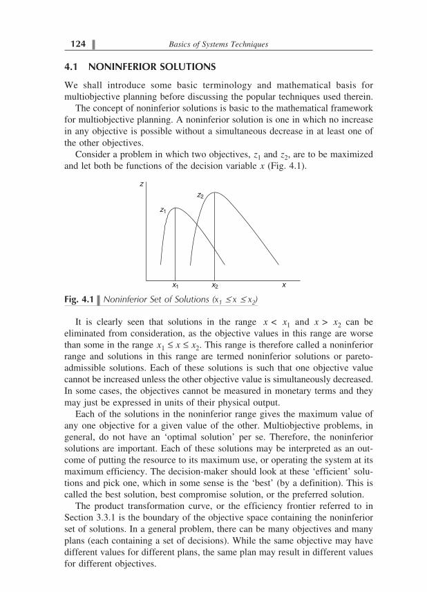
��� Basics of Systems Techniques
��� ����������� ������
We shall introduce some basic terminology and mathematical basis for
multiobjective planning before discussing the popular techniques used therein.
The concept of noninferior solutions is basic to the mathematical framework
for multiobjective planning. A noninferior solution is one in which no increase
in any objective is possible without a simultaneous decrease in at least one of
the other objectives.
Consider a problem in which two objectives, z1 and z2, are to be maximized
and let both be functions of the decision variable x (Fig. 4.1).
�������� ����������������������� ��������������
It is clearly seen that solutions in the range x < x1 and x > x2 can be
eliminated from consideration, as the objective values in this range are worse
than some in the range x1 � x � x2. This range is therefore called a noninferior
range and solutions in this range are termed noninferior solutions or pareto-
admissible solutions. Each of these solutions is such that one objective value
cannot be increased unless the other objective value is simultaneously decreased.
In some cases, the objectives cannot be measured in monetary terms and they
may just be expressed in units of their physical output.
Each of the solutions in the noninferior range gives the maximum value of
any one objective for a given value of the other. Multiobjective problems, in
general, do not have an ‘optimal solution’ per se. Therefore, the noninferior
solutions are important. Each of these solutions may be interpreted as an out-
come of putting the resource to its maximum use, or operating the system at its
maximum efficiency. The decision-maker should look at these ‘efficient’ solu-
tions and pick one, which in some sense is the ‘best’ (by a definition). This is
called the best solution, best compromise solution, or the preferred solution.
The product transformation curve, or the efficiency frontier referred to in
Section 3.3.1 is the boundary of the objective space containing the noninferior
set of solutions. In a general problem, there can be many objectives and many
plans (each containing a set of decisions). While the same objective may have
different values for different plans, the same plan may result in different values
for different objectives.

Multiobjective Planning ���
Let X be a vector of decision variables, X = (x1, x2, x3, … , xn), and Zj (X),
j = 1, 2, …, p denote p objectives, each of which is to be maximized. The
multiobjective problem may be written as
Maximize [Z1(X ), Z2(X ), …, Zp (X )]
subject to gi (X ) = bi i = 1, 2, …, m
The objective function in the problem is a vector consisting of p separate
objectives. The constraints impose technical feasibility. This objective function
in the vector form can be maximized only if it can be reduced to a scalar
function, using a value judgment analysis of the different components in it.
��� � ������� �����
There are two essential steps in multiobjective analysis: plan formulation and
plan selection. Plan formulation is aimed at generating the noninferior set of
solutions (or set of technologically efficient solutions), and plan selection is the
process of selecting the best compromise solution. Two of the most common
approaches in formulating a multiobjective planning problem are the weighting
method and the constraint method.
����� ����������������
In the weighting method, the objective function (in the vector form) is con-
verted to a scalar by expressing it as a weighted sum of the various objectives
by associating a relative weight to each objective function. If wj is the relative
weight assigned to the objective Zj, then the multiobjective model is written as
Maximize Z = w1Z1 + w2Z2 + … + wpZp
subject to gi(X ) = bi i = 1, 2, …, m
The relative weights, wj, reflect the trade-off or the marginal rate of transfor-
mation of pairs of objective functions. These weights are varied systematically,
and solutions obtained for each set of values. The solution obtained for a given
set of weights gives one generated set of noninferior or efficient solutions or
plans. By varying the weights in each case, a wide range of plans are obtained
for further analysis before the best one is selected.
Weights imply value judgments. The determination of the set of relative
weights is a complex exercise and has to be done keeping the preferences of
the decision-makers in mind who, in turn, are supposed to represent the interest
and preferences of the beneficiaries. This requires a study of the economic,
societal and developmental priorities. For a given set of weights, however, it is
easy to infer the relative values of the various objectives considered in the
analysis.
One major limitation of the weighting approach is that it cannot generate the
complete set of efficient plans unless the efficiency frontier is strictly convex.
If a part of it is concave, then, only the end points (and none on the curve in
between them) of this part can be obtained by the weighting technique.

��� Basics of Systems Techniques
����� ����� !����������
In this method, one objective is maximized, with lower bounds on all the others.
Maximize Zj (X )
subject to gi (X ) = bi i = 1, 2, …, m
and Zk (X ) � Lk for all k not equal to j
Any set of feasible values of Lk resulting in a solution with binding con-
straints gives an efficient alternative (solution). If the constrained method of
formulation can be solved using linear programming, it is particularly useful to
conduct sensitivity analysis to infer the implied tradeoffs for given right-hand
side values of the binding constraints. The dual variables of the binding con-
straints with Lk on the right-hand side are the marginal rates of transformation
of the objectives Zj (X ) and Zk (X ).
"!#$%������� Basic Problem Statement, following Loucks et al. 1981)
Let objective Z1(X ) = 5X1 – 4X2 and Z2(X ) = –2 X1 + 8X2. Both are to be
maximized. Assume the constraints on the variables X1 and X2 are
–X1 + X2 � 6
X1 � 12
X1 + X2 � 16
X2 � 8
X1, X2 � 0
1. Plot a pareto chart for admissible or noninferior solutions in decision
space.
2. Plot the efficient combinations of Z1 and Z2 in objective space.
3. Maximize Z1(X ) and Z2(X ) using the weighting method, given the weights
associated with Z1 and Z2 are 1 and 2 respectively, and illustrate the
method in decision and objective space.
4. Illustrate the constraint method of defining all efficient solutions in the
decision space.
Solution:
1. The decision space is plotted in the following figure. By plotting the
constraint boundary lines, we find that the boundary of the feasible
region is OBCDEF. The lines of constant Z1 and Z2 will be parallel to
the Z lines shown in the figure. However, the line of maximum Z1
passes through the point F(12,0), and that of maximum of Z2 through C
(2,8). This may be verified by comparing the slopes of the objective
lines with those of the constraint lines. For example, the slope of the
objective function line, Z1, is 5/4 (dx2/dx1 = 5/4), and the point on the
boundary of the feasible region, farthest from the origin, which a line
with this slope meets, is F. Similarly, Z2 is a maximum at the point C.
Therefore, the noninferior set of solutions are represented by the line
CDEF. Note that the segment BC does not contain noninferior solu-
tions, as both objectives Z1 and Z2 can be increased along BC (Z1 can be
increased from –24 to –22, and Z2 from 48 to 60, by moving from
B to C).

Multiobjective Planning ��&
2. Evaluating the values of Z1(X ) and Z2(X ) at C, D, E, and F, the line of
efficient combinations of Z1 and Z2 in the objective space is plotted.
This is the line CDEF in the following figure.
Decision Space
3. Weighting method
Maximize Z = w1Z1 + w2Z2
with w1 = 1 and w2 = 2
Z = Z1(X ) + 2Z2 (X ) = (5X1 – 4X2 ) + 2 (–2X1 + 8X2)
= X1 + 12X2
Objective is to maximize Z = X1 + 12X2, subject to the given con-
straints.
Decision space: The Z line, Z = X1 + 12 X2, has a slope of –1/12, in
the decision space and Z is found to have a maximum value equal to
104 on the boundary of the decision space at D (8,8). [The student may
verify this.]

��' Basics of Systems Techniques
Objective space: The objective function line Z = Z1 + 2Z2, has a slope of
–1/2. The value of Z will be maximum at D (8, 48) in the objective
space, and is equal to Z = 8 + 2(48) = 104.
4. Constraint method
The problem may be solved using LP.
Maximize Z1(X)
subject to Z2(X) ��L2, along with the other constraints.
Any optimal solution for an assumed value of L2 is a noninferior
solution, if the constraint with L2 on the right-hand side is binding. By
varying the value of L2, we get different noninferior solutions.
An easier way to identify different noninferior solutions is to solve
the following problem using LP.
Maximize Z1 = 5X1 – 4X2
subject to – X1 + 4X2 = L2
– X1 + X2 � 6
–X1 � 12
X1 + X2 � 16
X2 � 8
X1, X2 � 0
Solve for different values of L2 for which the problem is feasible. Each set
of the maximized Z1 value and the corresponding L2 (Z2 value) defines one
noninferior solution. The entire set of noninferior solutions may be obtained
by solving the problem for all feasible values of L2 (problems of this type can
be easily solved on a PC using PC software for LP such as LINGO).
Problems
4.2.1 A reservoir is planned both for gravity and lift irrigation through
withdrawals from its storage. The total storage available for both uses
is limited to 5 units each year. It is decided to limit the gravity irrigation
withdrawal in a year to 4 units. If X1 is the allocation of water to
gravity irrigation and X2 the allocation for lift irrigation, two objectives
are planned to be maximized and are expressed as
Z1 = 3X1 – 2X2
Z2 = –X1 + 4X2
1. Formulate a multiobjective planning model using weighting
approach with weights for gravity and lift irrigation withdrawals
being w1 and w2 respectively. Plot the decision space and the
objective space and determine the optimal share of withdrawals
for gravity and lift irrigations, if
(i) w1 = 1 and w2 = 2
(ii) w1 = 2 and w2 = 1.
2. Formulate the problem using the Constraint method.
[Ans: (i) X1 = 0; X2 = 5. (ii) X1 = 4; X2 = 0 to 1]

Multiobjective Planning ��(
4.2.2 Refer to Example 4.2.1 illustrated earlier. Assume that while
maximizing the weighted objective function, Z = w1 Z1 + w2 Z2, the
decision-maker chose the point E (X1 = 12, X2 = 4) in the decision
space as the preferred solution. Determine the value or range of
values of the marginal rate of substitution of the objective Z2 to Z1.
Interpret what it means in the perception of the decision maker.
[Ans: –10/9 > w1/w2 > –2]
��) � ���� �����
Plan selection depends essentially on the relative preferences of the decision
maker to the various objectives to be maximized. In the weighting method,
e.g., if the relative weights attached to each objective are specified then the
particular solution corresponding to those specified weights will be the selected
plan. However, determination of these relative weights itself is a problem in
multiobjective planning. Necessarily, multiobjective planning is an interactive
and iterative process involving decision makers and systems analysts. Quantifi-
cation of intrinsic preferences to different objectives is necessary for multi-
objective planning and this is where the systems analyst’s role comes into play.
There are a number of plan generation and selection techniques that warrant a
more elaborate discussion than is possible in an elementary book like this. The
publications mentioned at the end of the chapter may be consulted for further
reading on this.
���
1. Loucks, D.P., J.R. Stedinger, and D.A. Haith, Water Resource Systems
Planning and Analysis, Prentice-Hall, Inc., Englewood Cliffs, N.J. 1981.
2. Haimes, Y.Y., Hierarchical Analysis of Water Resources: Modeling and
Optimization of Large-Scale Systems, McGraw-Hill, Inc., New York, 1977.
3. Haimes, Y.Y., W.A. Hall, and H.T. Freedman, Multiobjective Optimiza-
tion of Water Resources Systems: The Surrogate Worth Trade-off Method,
Elsevier, Amsterdam, 1975.

���� �
���������������
� Reservoir Systems—Deterministic Inflow
� Reservoir Systems—Random Inflow

������� �
�����������������������������������
Areservoir is a storage structure that stores water in periods of excess flow
(over demand) in order to enable a regulation of the storage to best meet
the specified demands. Modelling a reservoir system, in general, is specific to
the system, and the assumptions one may use to make the model formulation
simple enough for problem-solving through known techniques in systems analy-
sis. This chapter illustrates how a reservoir may be modelled using determinis-
tic inputs. Model formulations for two important aspects of reservoir modelling
are discussed: reservoir sizing and reservoir operation.
��� �����������
The annual demand for water at a particular site may be less than the total
inflow there, but the time distribution of the demand may not match the time
distribution of inflow, resulting in surplus in some periods and deficit in some
other periods of the year. A reservoir serves the purpose of temporarily storing
water in periods of excess inflow and releasing it in periods of low flow so that
the demands may be met in all periods. The problem of reservoir sizing in-
volves determination of the required storage capacity of the reservoir when
inflows and demands in a sequence of periods are given. The total storage can
be divided into three components: dead storage (for accumulation of sedi-
ments), active storage (for conservation purpose such as water supply and
hydropower production), and flood storage (for reducing flood peak). While
each of these components may be determined by separate modelling studies,
we confine ourselves in this section only to the determination of the active
storage capacity of the reservoir.
The inflow to the reservoir is in fact a random variable. The problem gets
complicated if the randomness of the inflow has to be taken into account. Let
us consider the simpler case of deterministic inflow for the purpose of the
present discussion, and also assume that the given inflow sequence repeats

��� Model Development
itself. If the length of the inflow sequence is a year, it means that the inflow in
a given (within-the-year) period is the same in all the years.
One common method, extensively used in practice, is to determine the ac-
tive storage capacity using the Rippl diagram or the mass diagram by plotting
cumulative inflow with time. The method involves finding the maximum posi-
tive cumulative difference between a sequence of reservoir releases (equal to
demands) and historical inflows over a sequence of time periods in which the
demand is constant. For details of this method, the reader may refer any standard
textbook on hydrology. The procedure is shown in Fig. 5.1.
������� ����������������� ���������������������������� ���
If the demand is constant in each time period, the method is quite simple to
apply. When the demand varies across time periods, the procedure requires a
plot of the cumulative deficits in time from the period in which a deficit sets in,
for the duration of the deficit, and finding the maximum deficit among all such
durations. The total deficit duration containing this maximum deficit is known
as the critical period.
This method is still cumbersome compared to a simple analytical technique,
known as sequent peak method, which is described next. If we ignore the
evaporation losses in the reservoir, the sequent peak method is quite simple.
We shall first assume this situation and look at the algorithm to determine the
reservoir capacity by the sequent peak method (Section 5.1.1). Later, we shall
see how the reservoir losses can be incorporated into the method to determine
the active storage capacity of the reservoir.
����� ������������������������������ �!"#���"�
The sequent peak analysis can be applied for constant or varying demands in
time. In this method, we find the maximum cumulative deficit over adjacent
sequences of deficit periods, and determine the maximum of these cumulative
deficits. The inflow sequence is assumed to repeat and the analysis is carried

Reservoir Systems—Deterministic Inflow ���
out over two cycles, or two consecutive inflow sequences. If the critical period
lies towards the end of an inflow sequence, carrying out the analysis over two
cycles ensures the capture of the maximum value of the cumulative deficit,
which really is the required active storage capacity. The sequent peak algo-
rithm is as follows:
Let t denote the time period, Qt the inflow, and R t, the required release or
demand in period t. Let K t be defined as follows:
Kt = Kt–1 + Rt – Qt if positive,
= 0 otherwise,
with K0 set equal to zero (K0 = 0).
Or, Kt may be expressed conveniently as the maximum of zero and Kt–1 + Rt
– Qt, as
Kt = max {0, Kt–1 + Rt – Qt}
The values of K t are computed for each period t for two cycles or successive
inflow sequences.
Let K* = max {Kt} over all t. Then K * is the required active storage capacity
of the reservoir.
It may be noted that if the value of Kt is zero at the end of the last period of
the first cycle, then computations over the second cycle are not necessary. This
happens when the critical period is entirely contained in the first cycle itself.
Otherwise, the second cycle computations are required. Here again, computa-
tions of K for all the periods in the second cycle also are not necessary, beyond
a time period t for which the value of K is exactly the same as that in the first
cycle for the corresponding period (as in Table 5.1 in Example 5.1.1).
It may be noted that it is immaterial whether or not the historical inflow
sequence coincides with a calendar year or a water year. The important feature
is that computation of Kt over two consecutive cycles (inflow sequences) will
ensure that the correct value of K* is determined.
The sequent peak method is just an analytical procedure to determine the
maximum cumulative deficit that occurs over time, given the inflows and de-
mands across time periods. The method is very similar to the mass diagram
approach, when the evaporation losses in the reservoir are neglected.
It is obvious that if the total annual demand exceeds the total annual inflow,
no amount of reservoir storage would satisfy the full demand in all the periods
of a year. This is because of inflow limitation, or lack of available water.
�$�%!������� (Reservoir capacity with evaporation loss neglected)
Determine the required capacity of a reservoir whose inflows and demands
over a 6-period sequence are as given below (release, Rt = demand, Dt).
Period, t 1 2 3 4 5 6
Inflow, Qt 4 8 7 3 2 0
Demand, Dt (= Rt) 5 0 5 6 2 6
It is assumed that the sequence repeats itself. In this case, total inflow =
total demand in the six periods of the sequence and is equal to 24. Since

��& Model Development
evaporation loss is neglected, it is possible to determine the required storage
to meet the demands in full. In this case, release equals demand in each
period and there is no spill.
Table 5.1 illustrates the computations using the sequent peak algorithm.
'�(����� �������������������������������������� ���
t R t Qt Kt – 1 K a = Kt – 1 + Rt – Qt
1 5 4 0 1
2 0 8 1 0
3 5 7 0 0 � Reservoir full
4 6 3 0 3
5 2 2 3 3
6 6 0 3 9
1 5 4 9 10@ � Reservoir empty
2 0 8 1 2
3 5 7 2 0
4 6 3 0 3
5 2 2 3 3 repeats
a K is max [0, Kt–1 + Rt – Qt]@ max {Kt} = K *, the required capacity
The computations in the second cycle repeat after period 5 (hence, are not
shown). The required capacity of the reservoir is max {Kt} = 10.
Note: A reservoir of capacity of K* = 10 will be full at the end of the third
period, and will be empty at the end of the first period of the following
sequence (analyse why?). The intervening period is the ‘critical period.’
Constant demand: If the demand in each period is constant (say, for instance,
the water supply demand for a town), then Rt = R for all t in the above
formulation. It is to be noted that in the absence of losses, the maximum
constant demand, R, which can be met from a given sequence of inflows is
equal to the average of the inflows, Qt, over all t. A constant demand larger
than this magnitude cannot be met, whatever be the reservoir capacity, due to
inadequate quantum of inflow. In the example illustrated above, the maxi-
mum constant demand that can be met in a time period is 24/6 = 4 units of
water. Any higher value is infeasible due to limitation of the total quantum of
inflow, no matter what the reservoir capacity is.
����) �������������������*"���+�#���� �!"#���"�,"��
The sequent peak method can be modified (Lele, 1987) to take into account
storage-dependent losses in the determination of the reservoir capacity, with
some additional data and computations. The additional data required are the
evaporation rate in each time period and the area capacity curve of the reser-
voir. A procedure using sequent peak method is presented in this section,
which takes into account evaporation losses in the reservoir.

Reservoir Systems—Deterministic Inflow ��-
The reservoir storage continuity may be written as
St + Qt – Rt – Et = St + 1
where St is the active storage at the beginning of period t, Qt is the inflow
during period t, Rt is the release during period t, and Et is the evaporation loss
during period t.
Evaporation loss (in volume units) in a period is given by the product of the
evaporation rate (in depth units) and the average water spread area (average of
the water spread areas at the beginning and at the end of the period) of the
reservoir in that period. The water spread area is a function of the total storage
(dead + active) in the reservoir. The reservoir level will always be above the
dead storage level. If water spread area is plotted against reservoir storage, the
relation between the water spread area above the dead storage level and the
active storage (storage above the dead storage) can, in most cases, be approxi-
mated by a straight line (Loucks et al., 1981), as in Fig. 5.2.
������) ����!��������"�����������������#���������������������
The evaporation loss in period t then is given by
Et = et At, where At = Ao + a (St + St + 1)/2, or
Et = Lt + at (St + St + 1)
where Lt is the fixed evaporation loss = et Ao, et is the evaporation rate in
period t, Ao is water surface area at the top of the dead storage level, at = aet/2,
and ‘a’ is the surface area per unit active storage, or the slope of the straight
line segment with water surface area (y-axis) plotted against reservoir storage
(x-axis), Fig. 5.2.
The storage continuity equation, taking into account evaporation loss, thus
becomes
(1 – at ) St + Qt – Lt – R t = (1 + at) St +1
This equation defines the relationship between the active storages at the
beginning and at the end of period t. The algorithm (Lele, 1987) to determine
the required capacity of the reservoir is given by the following steps.
������ �����������
1. Record the data: Qt, Rt, et, A0, and a.
2. Et = 0 for all t = 1, 2, …, T, where T is the last period of the inflow
sequence.

��. Model Development
����� ���������������������
1. K0 = 0
2. Calculate Kt = max {0, Kt – 1 + Rt + Lt – Qt} for all t = 1, 2, …, T
3. If KT = K0, then go to 4; else if this is the first iteration in Step 2, then put
K0 = KT and go to 2; else STOP. Sequent peak analysis failed as the gross
demand is greater than the average inflow.
4. Find the period for which Kt is maximum over all t = 1, 2, …, T, and call
this period ICRIT. This is the period at the end of which the reservoir will
be empty.
5. Search backward from t = ICRIT until Kt = 0 is encountered for the first
time. Call this period, for which Kt = 0, as IOVF. This is the period at the
end of which the reservoir will be full.
������ ���������
1. SICRIT +1 = 0.
2. From t = ICRIT, move backward to t = IOVF +1, calculate St = [St +1(1+ at)
+ Rt + Lt – Qt]/(1 – at).
3. K* = SIVOF +1.
������ ��������
1. For t = ICRIT + 1 forward to t = IVOF – 1, calculate
St +1 = min {K*, [St (1 – at) + Qt – R t – Lt]/(1 + at)}
2. If any St is negative, then go to 3 (the sequent peak procedure should be
repeated with new values of evaporation losses, Et, using the current val-
ues of St); else STOP. K* is the required active storage.
3. Calculate Et = et [a(St + St +1)/2 + A0] for all t = 1, 2, …, T and go back to
Step 2.
The required reservoir capacity will be naturally higher, when the evapora-
tion loss is taken into account, than when it is not.
�$�%!������) (Reservoir capacity with evaporation loss considered)
The monthly inflows (Qt) and demands (Dt), in Mm3, and evaporation rate, et,
in mm for a reservoir are given below.
June July Aug Sept Oct Nov
Qt 70.61 412.75 348.40 142.29 103.78 45.00
Dt 51.68 127.85 127.85 65.27 27.18 203.99
et 231.81 147.57 147.57 152.14 122.96 121.76
Dec Jan Feb Mar Apr May
Qt 19.06 14.27 10.77 8.69 9.48 18.19
Dt 203.99 179.47 89.76 0 0 0
et 99.89 97.44 106.14 146.29 220.97 246.75
Reservoir data: Area at dead storage level, A0 = 37.01 Mm2; Slope, a =
0.117115
The computations are shown in the following table (Table 5.2).

Reservoir Systems—Deterministic Inflow ���
The required reservoir capacity, when evaporation losses are neglected, is
588.11 Mm3; whereas, with evaporation losses taken into account, the re-
quired capacity works out to 617.986 Mm3.
�$�%!�������1. Compute the active storage capacity of a reservoir to supply a constant
maximum annual yield, given the following sequence of annual flows:
{8, 4, 6, 2, 4, 6}
2. Assume a year has two distinct seasons, wet and dry. Eighty per cent of
annual flow occurs in the wet season each year, and eighty per cent of
annual yield is demanded in the dry season each year. Determine the
percentage increase in the required storage capacity compared to 1 above.
Use the sequent peak method, neglecting evaporation and seepage
loss.
Solution:
Assuming the annual inflow sequence repeats, the maximum constant yield
possible (without losses) = average annual inflow = (8 + 4 + 6 + 2 + 4 + 6)/6
= 5.
1. The following table shows the computations of Kt in each period.
K0 = 0
Period, t Rt = release Qt = inflow Kt = max {0, Kt –1 + Rt – Qt }
1 5 8 0
2 5 4 1
3 5 6 0
4 5 2 3
5 5 4 4 (maximum)
6 5 6 3
1 5 8 0
In this example, computations can stop after period 1 in the second
cycle as the value of K t for period 1 is the same (= 0) as that for the
period 1 in the earlier cycle. The entries for the subsequent periods
simply repeat (as those for the corresponding periods in the first cycle).
Required active storage capacity = max {K t} = 4.
With this capacity, the reservoir will be full at the end of the first
and third periods and will be empty at the end of the fifth period
(verify). Hint: Examine St + Qt – R t = St +1 over a few cycles (sequences)
starting from any initial storage, St, in any period, t, till steady state is
reached, i.e., St for given t is the same in different cycles.
2. Inflow in the wet season = 0.8 (annual flow) each year, and inflow in
the dry season = 0.2 (annual flow) each year.
Demand in the wet season = 0.2 (5) = 1 each year, and
demand in the dry season = 0.8 (5) = 4 each year.

��) Model Development
Sequent peak method is applied to the 6-year (12 seasons) sequence.
For the sequent peak method, one cycle, therefore, has 12 seasons (6
years).
The following table shows the computations.
Kt = 0 = K0 = 0
Period Rt Qt K t = max {0, K t –1 + Rt – Qt }
1 wet 1 6.4 0.0
Dry 4 1.6 2.4
2 wet 1 3.2 0.2
Dry 4 0.8 3.4
3 wet 1 4.8 0.0
Dry 4 1.2 2.8
4 wet 1 1.6 2.2
Dry 4 0.4 5.8
5 wet 1 3.2 3.6
Dry 4 0.8 6.8 (maximum)
6 wet 1 4.8 3.0
Dry 4 1.2 5.8
1 wet 1 6.4 0.4
Dry 4 1.6 2.8
2 wet 1 3.2 0.6
Dry 4 0.8 3.8
3 wet 1 4.8 0 (repeats)
The required storage capacity is max {Kt} = 6.8, an increase of 2.8
over the case in 1, which is an increase of (6.8 – 4.0)/4 = 0.7 or 70%.
This example clearly shows that, the capacity requirement increases
when the variations in inflow and demands within the year periods are
considered, rather than when the capacity is computed based on the
annual values alone.
The sequent peak method does not require any optimization software. Evapo-
ration accounting can easily be incorporated with some additional computa-
tions. But even without evaporation, the algorithm is not readily adaptable to a
system with more than one reservoir. Mathematical programming tools provide
such a capability. For example, it is more elegant to solve the problem of
determining the reservoir capacity with evaporation loss taken into account
using linear programming. The result, i.e. the required active storage capacity,
of course, should be the same irrespective of the method used—sequent peak
or linear programming. It may be noted that the linearity assumption of area
with storage is not necessary in the sequent peak method as long as the evapo-
ration loss is expressed as a known function of the storage. In LP, however, the
linearity assumption simplifies incorporating the evaporation loss function eas-
ily into storage continuity relationships.

Reservoir Systems—Deterministic Inflow ���
����� ����# "�#*�!�����/����,����#�#"�#�%%���
We shall discuss here how linear programming can be used to determine the
required active storage capacity of a single reservoir with evaporation losses
taken into account. The demand may be constant or varying with time. This is
an alternate method and is more elegant than the sequent peak method for
solving the same problem.
�����������������������
It is assumed, for the purpose of present discussion, that inflows are determin-
istic (known) and the sequence of inflows repeats itself in time.
There are two sets of constraints to be satisfied; one relates to storage
continuity and the other to the capacity. Let Rt be release (variable) and Dt, the
specified demand.
Constraints The storage continuity constraint is
(1 – at) St + Qt – Lt – R t = (1 + at) St +1 for all t
The storage in each period is bound by the capacity, K, thus,
St � K for all t; Also Rt � Dt for all t
The reservoir capacity K is a variable, which must be minimized. The objec-
tive then is to minimize K.
The model formulation thus reduces to:
Minimize K
subject to (1 – at) St + Qt – Lt – R t = (1 + at) St +1 for all t,
St � K for all t; Rt � Dt for all t.
ST +1 = S1, where T is the last period in the sequence.
The last constraint means that when we have a sequence of monthly inflows
for a year, T = 12, S13 in the formulation is set equal to S1. The purpose is to
ensure that the storage at the end of the last period in the year is the same as the
storage at the beginning of the first period, as the inflow sequence is assumed
to be repetitive. In the storage continuity equation written above, spill, if any in
period t, is absorbed in the term R t.
The problem can be very easily solved on a personal computer by using LP
software such as LINGO (Language for INteractive General Optimization,
LINDO Systems Inc., Chicago, Illinois, USA).
�$�%!������� (Reservoir capacity with evaporation neglected, using LP)
The following is the LP formulation of the problem (Example 5.1.1), solved
earlier by the sequent peak method, neglecting evaporation.
Period, t 1 2 3 4 5 6
Inflow, Qt 4 8 7 3 2 0
Demand, Dt (= Rt) 5 0 5 6 2 6
The problem formulation is:
Objective Function:
Minimize K
Constraints:
S1 + 4 – 5 = S2

��� Model Development
S2 + 8 – 0 = S3
S3 + 7 – 5 = S4
S4 + 3 – 6 = S5
S5 + 2 – 2 = S6
S6 + 0 – 6 = S1
S1 � K; S2 � K: S3 � K; S4 � K; S5 � K; S6 � K
Solving using LP, the optimal solution is K = 10.
�$�%!�� ����� (Reservoir capacity with evaporation loss considered using
LP.)
The example problem earlier mentioned under sequent peak method (Ex-
ample 5.1.2) can now be solved using linear programming.
The monthly inflows (Qt) and demands (Dt), in mm3, and evaporation rate, et,
in mm for the reservoir are given below.
June July Aug Sept Oct Nov
Qt 70.61 412.75 348.40 142.29 103.78 45.00
Dt 51.68 127.85 127.85 65.27 27.18 203.99
et 231.81 147.57 147.57 152.14 122.96 121.76
Dec Jan Feb Mar Apr May
Qt 19.06 14.27 10.77 8.69 9.48 18.19
Dt 203.99 179.47 89.76 0 0 0
et 99.89 97.44 106.14 146.29 220.97 246.75
Reservoir data: Area at dead storage level, A0 = 37.01 Mm2; Slope, a = 0.117115
Since equality form of constraints are used, it is important to distinguish
between the demand, Dt, and the release, Rt, in formulating constraints. As
the demands have to be met in every period, the lower bound for Rt is Dt, or
Rt � Dt for all t, which must be specified as additional constraints in the
model formulation. This inequality will take care of any spill necessary in a
period in addition to meeting the demand in full.
The LP model, with notation defined earlier, therefore, is,
Minimize K
subject to
(1 – at) St + Qt – Lt – Rt = (1 + at) St +1 for all t,
St � K for all t,
Rt � Dt for all t,
ST +1 = S1
When solved using LP, the optimal solution for K = 617.986 Mm3 (which
is the same as K, obtained in the sequent peak method, earlier, Table 5.2).
Also, if et is set equal to zero for all t, the LP solution yields K = 588.11 Mm3,
which is the required capacity when evaporation loss is neglected, as obtained
earlier using sequent peak method (Table 5.2). Verify the results in both cases
using a PC software such as LINGO.

Reservoir Systems—Deterministic Inflow ���
������������������ ���������!�������
The following points are of interest in linear programming formulations dis-
cussed earlier. These have to do basically with the ways in which the reservoir
storage continuity constraints are structured.
1. Equality Form of Constraints Consider the equality constraint
(1 – at) St + Qt – Lt – Rt = (1 + at) St +1 for all t.
The constraint should imply that Rt includes the demand to be met and
possible spill in the period t. In order to ensure that demand in every period is
satisfied in full, additional constraints, Rt � Dt, may be introduced in the
formulation, still retaining spill, if any, in period t, to be absorbed in the term Rt.
2. Inequality Constraints A simple alternative to using the equality con-
straints for storage continuity is to use the greater than or equal to sign (�) in
place of the equality sign (=) in the continuity constraints, and substitute the
demand Dt in place of R t, as
(1 – at) St + Qt – Lt – Dt � (1 + at) St +1 for all t
This form of specifying the constraints builds in flexibility to take care of
spills, where necessary. It ensures that the demand is met in full and provides
for any spill in periods of high flow. Note that spill can occur only when the
capacity is reached. The formulation will ensure that the excess water over the
demand and evaporation in any period will be stored in the reservoir itself, if
the reservoir is not full (in which case there is no spill), or will be stored up to
the reservoir capacity and the rest spilled. The inequality form is the most
convenient form of specifying the storage constraints. The problem statement
thus is:
Minimize K
subject to
(1 – at) St + Qt – Lt – Dt � (1 + at) St +1 for all t
and
St � K for all t
The spill in period t, Spillt, in this formulation will be equal to
Spillt = (1 – at) St + Qt – Lt – Dt – at St +1 – K, if positive,
= 0, otherwise.
3. Other Equality form of Constraints (i) Specify an additional term for spill
in each constraint and penalize spills in the objective function.
(1 – at) St + Qt – Lt – Dt – Spillt = (1 + at) St +1, for all t
The objective function is modified as
Minimize tt
K M Spill� �
�� �
� , where M is an arbitrarily large number.
Here also, full demands will be met in each period and spills will be mini-
mized, while minimizing the reservoir capacity. If the term, Spillt is not intro-
duced into the objective function, it is possible for Spillt to be positive even
when the reservoir does not reach the capacity at the end of the period, which
is physically meaningless.

��& Model Development
����� ��"#���0���+������"�12�$�%�%0���+�#"(��%3
In Section 5.1.3, we discussed the problem of determining the minimum reser-
voir capacity for given demands. A complementary problem is to determine the
maximum yield (the quantum of water that can be taken out of storage per
period, assumed constant) from a reservoir of given capacity. While the former
is a problem in planning and design, the latter is one of determining what best
can be expected from an existing reservoir. This is of interest in evaluating the
performance of an existing reservoir in terms of its expected yield.
Let the objective be to maximize the yield, R (per period), from a reservoir
of given capacity, K. Then the following formulation for the problem can be
used for LP.
Maximize R
subject to
(1 – at) St + Qt – Lt – R � (1 + at) St +1 for all t
and
St � K for all t
with T + 1 = 1, where T is the last period.
K is given, and R is to be determined.
��"�������������� ���������#����"��������$���
Making use of integer variables in LP formulation is an elegant way to solve
the problem using equality constraints with Dt, and explicitly accounting for
spills. The mixed integer formulation ensures that spill will not occur unless
the reservoir is full. This is done by introducing additional constraints.
Introduce additional constraints into the formulation as follows:
Spillt � �t Spillmax, where Spillmax is the maximum possible spill in any
period (as Spillmax cannot exceed the maximum monthly inflow in the year, the
latter may be used in place of Spillmax). Alternatively, the constraints may be
specified as
Spillt � �t M, where M is an arbitrary large constant.
�t � St + 1/K
�t is integer � 1
These constraints satisfy that
when St +1 is less than the capacity K, then �t = 0, and Spillt = 0, and
when St +1 is higher than the capacity, K, then St + 1/K is greater than 1. But St +1
is constrained to be no greater than K, because of the capacity constraint, with
the result �t will be forced to be equal to 1, in order to make Spillt positive (in
which case, St +1 equals K). Then all the three sets of constraints mentioned
above are consistent.
Thus the mixed integer LP formulation for maximizing yield is
Maximize R
subject to
(1 – at) St + Qt – Lt – R – Spillt = (1 + at) St + 1 for all t
Spillt � �t M, where M is an arbitrary large constant

Reservoir Systems—Deterministic Inflow ��-
�t � St +1/K
�t is integer � 1
St � K for all t,
and St +1 = S1.
In all these cases, it must be noted that if the data are such that the total
annual inflow in all the periods in the sequence is less than the sum of the
demands and evaporation losses, LP obviously gives an infeasible solution. In
this case, the demands cannot be satisfied in full in all periods, no matter how
large is the reservoir capacity, simply because of inflow limitation. If the in-
flow in each period is higher than the demand, however, we need neither
storage nor reservoir.
There is a maximum value of R associated with each K, and a minimum
required capacity, K, with each R. If one is given the other can be found.
However, it must be noted that the problem of determining K for a given R
cannot be solved using the mixed integer formulation. In the mixed integer
formulation, the constraint
�t � St +1/K, or �t K � St
becomes nonlinear when both �t and K are variables, as in the capacity deter-
mination problem. This does not apply for the yield determination problem, as
K is given and R is to be determined.
Storage Yield Function A plot of K for different values of R is called a
storage yield function. This will be an increasing function of R, up to some
maximum feasible value of R. Beyond this, the problem becomes infeasible,
meaning there is not enough water to yield R in full in each period. The upper
bound for R is because of the inflow limitation. Building a reservoir beyond the
capacity, corresponding to the upper bound of R, is a waste, as it does not
contribute to any additional yield.
Model formulation for determining required reservoir capacity to meet
given demands at specified reliability is presented in Section 6.3, and an
example application with model formulation for multiple crops is presented in
Section 7.3
Problems
5.1.1 Determine the required capacity (K) of the reservoir for each of the
given annual yields, given inflow data for a 6-year repetitive sequence,
as shown in the following table. Use LP, neglecting evaporation losses.
Plot the storage yield function. Verify that the required values of K
are as given in the last row of the table.
Year 1 2 3 4 5 6
Inflow 16 8 12 4 8 12
Yield 5 6 7 8 9 10
Min. K 1 2 3 4 6 8

��. Model Development
5.1.2 Consider the 12-month data given in Example 5.1.5. Use LP to deter-
mine the reservoir capacity using
(a) storage continuity constraints of the greater than or equal to type,
with demands as lower bounds for releases,
(b) storage continuity constraints in the equality form, incorporating
demands and spills explicitly, and penalizing spills in the objec-
tive function,
(c) storage continuity constraints in the equality form, incorporating
demands and spills explicitly, and using mixed integer LP,
(In all the three cases, you should get the same answer)
5.1.3 A reservoir is planned to supply water at a constant rate per season to
an industry. The reservoir inflows in the four seasons of a year are
1500, 800, 1200, and 500, respectively, and repeat every year. Con-
sider evaporation loss from the reservoir in any season to be 5% of
the average storage in that season. Neglect all other losses. Formulate
and solve an LP model to determine the constant maximum rate of
water supply per season, if the reservoir capacity is 450 units.
(Ans. 938.75)
5.1.4 A reservoir is to be constructed to supply water at a maximum con-
stant rate per season for a city. The inflows in the six seasons of the
year are 3, 12, 7, 3, 2, and 3, respectively. Determine the minimum
required reservoir capacity using sequent peak method. Neglect all
losses. (Ans. 9)
5.1.5 In general, if the storage continuity constraints are used as expressed
below, in the LP formulation to determine reservoir capacity,
(1 – at) St + Qt – Lt – Dt � (1 + at) St +1 for all t,
analyze the nature of the solution for feasibility.
(Hint: First analyze the case without evaporation losses).
��) �������������'��
A reservoir operating policy is a sequence of release decisions in operational
periods (such as months), specified as a function of the state of the system. The
state of the system in a period is generally defined by the reservoir storage at
the beginning of a period and the inflow to the reservoir during the period.
Once the operating policy is known, the reservoir operation can be simulated in
time with a given inflow sequence. A number of optimization algorithms have
been developed for deriving reservoir operating policies. However, the most
common policy implemented in practice is the so-called standard operating
policy, which is discussed first in this section. This policy by itself is not based
on or derived from any optimization algorithm.
��)�� ����+�#+�!�#������"����
The standard operating policy (SOP) aims to best meet the demand in each
period based on the water availability in that period. It thus uses no foresight
on what is likely to be the scenario during the future periods in a year. Let D

Reservoir Systems—Deterministic Inflow ��4
and R represent, respectively, the demand and the release in a period. Let the
capacity of the reservoir be K. Then the standard operating policy for the
period is represented as illustrated in Fig. 5.3. The available water in any
period is the sum of the storage, S, at the beginning of the period, and the
inflow Q during the period. The release is made as per the line OABC in the
figure.
Figure 5.3 implies the following:
Along OA: Release = water available; reservoir will be empty after release.
Along AB: Release = demand; excess water is stored in the reservoir (filling
phase).
At A: Reservoir is empty after release.
At B: Reservoir is full after release.
Along BC: Release = demand + excess of availability over the capacity (spill)
In other words, the release in any time period is equal to the availability, S +
Q, or demand, D, whichever is less, as long as the availability does not exceed
the sum of the demand and the capacity. Once the availability exceeds the sum
of the demand and the capacity, the release is equal to demand plus excess
available over the capacity. It is to be noted that the releases made as per the
standard operating policy are not necessarily optimum as no optimization crite-
rion is used in the release decisions. For highly stressed systems (systems in
which water availability is less than the demand in most periods), the standard
operating policy performs poorly in terms of distributing the deficits across the
periods in a year.
With evaporation loss E included, the standard operating policy may be
expressed as
Rt = Dt if St + Qt – Et � Dt
= St + Qt – Et, otherwise
Ot = (St + Qt – Et – Dt) – K if positive
= 0 otherwise
St + 1 = St + Qt – Et – Rt – Ot, with Rt and Ot determined as above
������� ���������$������������� �

��5 Model Development
St is the storage at the beginning of the period t, Qt is the inflow during the
period t, Dt is the demand during the period t, Et is the evaporation loss during
the period t, R t is the release during the period t, and Ot is the spill (overflow)
during the period t. Note that St +1 = K, if Ot > 0.
�$�%!�� ��)�� An illustrative example of the standard operating policy is
shown in Table 5.3, for a reservoir with capacity K = 350 units and an initial
storage of 200 units. Inflow Qt, demand Dt and evaporation Et are known
values, as given in the table.
'�(����� ����������$���������%�������������$������������� ����$�
K = 350
t St Qt Dt Et Rt St+1 Ot
1 200.00 70.61 51.68 10 51.68 208.93 0.00
2 208.93 412.75 127.85 8 127.85 350.00 135.83
3 350.00 348.40 127.85 8 127.85 350.00 212.55
4 350.00 142.29 65.27 8 65.27 350.00 69.02
5 350.00 103.78 27.18 6 27.18 350.00 70.60
6 350.00 45.00 203.99 6 203.99 185.01 0.00
7 185.01 19.06 203.99 5 199.07 0.00 0.00
8 0.08 14.27 179.47 5 9.27 0.00 0.00
9 0.00 10.77 89.76 6 4.77 0.00 0.00
10 0.00 8.69 0.00 8 0.00 0.69 0.00
11 0.69 9.48 0.00 8 0.00 2.17 0.00
12 2.17 18.19 0.00 10 0.00 10.36 0.00
��)�) �!��%���!�#������"����/����,�
One of the classical problems in water resources systems modelling is the
derivation of an optimal operating policy for a reservoir to meet a long-term
objective. Modelling techniques to be used depend on whether the reservoir
inflows are treated deterministic or stochastic. In this chapter only the case of
deterministic inflows is dealt with. Operating policies considering stochastic
inflows are discussed in Chapter 6.
Given a reservoir of known capacity K, and a sequence of inflows, the
reservoir operation problem involves determining the sequence of releases Rt,
that optimizes an objective function. In general, the objective function may be
a function of the storage volume and/or the release. A single, simplified reser-
voir system is represented as shown in Fig. 5.4.
InflowQt
ReservoirCapacity, K
Evaporation, Et
ReleaseRt
������� �����������������$��������

Reservoir Systems—Deterministic Inflow ���
��� ��������
Consider the simplest objective of meeting the demand to the best extent pos-
sible (the same objective as considered in the standard operating policy), such
that the sum of the demands met over a year is maximum. This may be formu-
lated as a LP problem as follows:
Max tt
R� (5.2.1)
Subject to
St +1 = St + Qt – Rt – Et – Ot �t (5.2.2)
Rt � Dt �t (5.2.3)
St � K �t (5.2.4)
Rt � 0 �t (5.2.5)
St � 0 �t (5.2.6)
ST +1 = S1 (5.2.7)
where T is the last period in the year, and all other terms are as defined in
Section 5.2.1.
The constraint (5.2.3) restricts the release during a period to the correspond-
ing demand, while the objective function (5.2.1) maximizes the sum of the
releases. Thus the model aims to make the release as close to the demand as
possible over the year. To ensure that the overflows Ot assume a nonzero value
in the solution only when the storage at the end of the period is equal to the
reservoir capacity, K, integer variables may be used as discussed in Section
5.1.4. Constraint (5.2.7) makes the end of the year storage equal to the begin-
ning of the (next) year’s storage, so that a steady state solution is achieved.
When the initial storage at the beginning of the first period is known, an
additional constraint of the form, S1 = S0, may be included, where S0 is the
known initial storage, in which case the sequence of releases obtained would
be optimal only with respect to the particular initial storage. The end of the
year storage, ST +1, may be set equal to the known initial storage (5.2.7), if a
steady state solution is desired, or may be left free (i.e. constraint 5.2.7 is
excluded) if only the release sequence for one year, with known initial storage,
S0, is of interest.
�$�%!����)�) Table 5.4 below is constructed with results obtained by solv-
ing the LP model (5.2.1) to (5.2.7) with inflow Qt, demand Dt, and evapora-
tion Et values used in Example 5.2.1.
'�(����� ����������$�������������������"�������&�������
t St Qt Dt Rt Et St+1 Ot
1 10.36 70.61 51.68 51.68 10 19.29 0.00
2 19.29 412.75 127.85 127.85 8 296.19 0.00
3 296.19 348.40 127.85 127.85 8 350.00 158.74
4 350.00 142.29 65.27 65.27 8 350.00 69.02
5 350.00 103.78 27.18 27.18 6 350.00 70.60
(Contd)

��) Model Development
(Contd)
t St Qt Dt Rt Et St+1 Ot
6 350.00 45.00 203.99 39.00 6 350.00 0.00
7 350.00 19.06 203.99 108.87 5 255.19 0.00
8 255.19 14.27 179.47 179.47 5 84.99 0.00
9 84.99 10.77 89.76 89.76 6 0.00 0.00
10 0.00 8.69 0.00 0.00 8 0.69 0.00
11 0.69 9.48 0.00 0.00 8 2.17 0.00
12 2.17 18.19 0.00 0.00 10 10.36 0.00
Note that the values of Rt in Tables 5.3 and 5.4 are not expected to be identical, as the two
policies are not strictly identical.
Rule Curves for Reservoir Operation Reservoir operation rules are guides
for those responsible for reservoir operation. They apply to reservoirs which
are to be operated in a steady state condition. A rule curve indicates the
desired reservoir release or storage volume at a given time of the year. Some
rules identify storage volume targets that the operator is to maintain, as far as
possible, and others identify storage zones, each associated with a particular
release policy. The rule curves are best derived through simulation for a
specified objective, although for some simple cases, it may be possible to
derive them using optimization.
In Example 5.2.2 given earlier, the end of period storages, St +1, define the
rule curve. They are the desired end-of-period storages (target storages) to be
maintained in operating the reservoir in different time periods.
The resulting rule curve is as shown in Fig. 5.5. Note that if the objective
function is changed, in general, a different rule curve is obtained.
������� ���������������������"����!�����'#(#(
���������%����&�������
A multireservoir system operation problem may be similarly formulated as an
LP problem. Consider, for example, the three-reservoir system shown in
Fig. 5.6. The system serves the purposes of water supply, flood control and
hydropower generation. Release for water supply is passed through the

Reservoir Systems—Deterministic Inflow ���
powerhouse generating power, and losses in the powerhouse are negligible.
Benefits from hydropower are expressed as a function of storage alone. 1 2,i it tB B
and 3itB , are respectively the net benefits associated with unit release, unit
available flood freeboard (= reservoir capacity – available storage), and unit
storage for reservoir i in period t. A portion �1 and �2 of the release made at
reservoirs 1 and 2 respectively add to the natural inflow of reservoir 3. Further,
a minimum flood storage miniF needs to be ensured during flood season at the
reservoir i. Maximum release that may be made at reservoir i is maxiR . It is
assumed, in the following illustration, that
11it tB B �i
22it tB B �i
and 33it tB B �i
The LP problem may be stated as
31 2 3
1 1
max ( )T
i i it t t i t t t
i t
B R B K S B S
� �� � �� �� �
subject to
1i i i i i it t t t t tS S Q R E O� � � � � �t, i = 1, 2
1 21 1 2
i i i i i it t t t t t t tS S Q R R R E O� �� � � � � � � �t; i = 3
itS � Ki i = 1, 2, 3; �t
Ki – itS � min
iF �i; �t � Flood Season
itR � max
iR
������& ���������������$������������)��
K
St

��� Model Development
1 1i iTS S�
0; 0.i it tS R� �
In the model, the index i refers to a reservoir (i = 1, 2, 3), and t to time period
(t = 1, 2, …, T). Q is the natural inflow, K is reservoir capacity, S is storage, R
is release, E is evaporation, and O is overflow (spill). The storage St is the
storage at the beginning of period t.
�$�%!����)�� Consider the data given in the table below for a three-period,
three-reservoir system. The reservoir system configuration is as shown in
Fig. 5.6.
Reservoir Inflow K Fmin *1B *
2B *3B
t = 1 t = 2 t = 3 t = 1 t = 2 t = 3
1 25 10 15 10 3 2 7 50 10 25
2 10 30 15 15 2 3 4 60 10 30
3 20 12 15 20 2 3 5 70 10 35
*The benefit coefficients B1, B2, and B3 are assumed constant for all three periods.
�1 = 0.2 and �2 = 0.3
The solution of the LP problem is as follows:
Reservoir 1 Reservoir 2 Reservoir 3
t = 1 t = 2 t = 3 t = 1 t = 2 t = 3 t = 1 t = 2 t = 3
St 0.0 8.0 3.0 2.0 12.0 11.0 0.0 17.0 15.0
Rt 17.0 15.0 18.0 0.0 31.0 24.0 6.4 26.3 40.8
(K – St)* 10.0 2.0 7.0 13.0 3.0 4.0 20.0 3.0 5.0
*(K–St) is the available flood storage in period t.
Note that the spill from a reservoir is included in the release values shown
for that reservoir. Also note that the mass balance for reservoir 3 includes the
contributions from the two upstream reservoirs. In this hypothetical example,
the benefit coefficients for the release are much higher than those for the
flood storage. The solution will be quite sensitive to variations in these coeffi-
cients. It would be instructive for the student to generate and analyze a num-
ber of solutions, varying the benefit coefficients relative to each other, for the
same inflow data provided in this example.
��)�� �����"��#��"����/����6�
A general reservoir operation problem is to derive a stationary policy for a
repeating sequence of inflows {Qt} every year, where t is a ‘within-year’ period,
i.e. less than one year. The stationary policy, which may be derived using DP,
specifies the release as a function of the storage in a period. The objective is to
derive an operating policy which results in the maximized annual net benefit in
the long run (steady state).

Reservoir Systems—Deterministic Inflow ���
As shown in Fig. 5.7, the computations start at some distant year in the
future in the last period, T. The choice of this year is such that the computations
yield a steady state solution in the end. The computations are similar to those
carried out for the single year policy discussed in Sec. 2.3.5 with the following
modifications:
������- ����� �����������"������������������ �
1. There are no boundary conditions. The initial (beginning of the year) or
the final (end of the year) storage values are not specified, and we seek the
policy for all possible storage states.
2. The computations extend beyond the one year horizon, with the stage
index n continuously increasing from n = 1, 2, …, T, T + 1,T + 2, …, and
the period index, t, keeping track of the position of the particular stage
within the year, t = T, T – 1,…, 1 (Fig. 5.7).
3. The computations are carried out until the solution reaches a steady state.
The steady state is said to be reached at stage n, when the annual net
benefit given by [ ( ) ( )]� �n T n
t t t tf S f S converges to a constant value, for
all St, where ( )nt tf S is the accumulated net benefit up to (and including)
stage n. This implies that the net benefit over the next T periods from
stage n is a constant for all possible initial storages at that stage.
The general recursive equation is written as
( )nt tf S =
11max [ ( , ) ( )]
nt t t t t ttB S R f S Q R
��� � �
0 � R t � St + Qt
St + Qt – R t � K
where Bt(St, R t) is the objective function value in period t for specified storage,
St, at the beginning of the period t, and R t, the release during period t. K is the
known reservoir capacity and Qt is the inflow during period t.
�$�%!����)�� The steady state policy is derived for the example discussed
in Section 2.3.5. The first year computations are the same as the complete
solution for the annual problem discussed earlier, with the addition that, in the
last stage, n = 4 (t = 1), we solve for all values of S1, instead of the specified
value 0. The following tables give summary results of the computations,
starting from Year 1 and proceeding in the backward direction.

��& Model Development
������ ������
n = 1 t = 4 Qt = 2 n = 5 t = 4 Qt = 2
S414f (S4 ) *
4R S45
4 4( )f S *4R
0 320 2 0 1780 1, 2
1 480 3 1 1940 1, 3
2 520 4 2 2010 1, 2, 3
3 520 4, 5 3 2170 1, 3
4 520 4, 5 4 2240 2, 3
�������������# �������������#
n = 2 t = 3 Qt = 3 n = 6 t = 3 Qt = 3
S32
3 3( )f S *3R S3
63 3( )f S
*3R
0 800 2, 3 0 2260 1, 2, 3
1 960 3 1 2420 1, 3
2 1000 3, 4 2 2490 1, 2, 3
3 1040 4 3 2560 2, 3
4 1040 4, 5 4 2720 3
n = 3 t = 2 Qt = 1 n = 7 t = 2 Qt = 1
S23
2 2( )f S *2R S2
72 2( )f S *
2R
0 1050 1 0 2510 1
1 1210 1 1 2670 2
2 1280 2, 3 2 2740 1, 2, 3
3 1440 3 3 2900 3
4 1480 3, 4 4 2970 1, 3
n = 4 t = 1 Qt = 2 n = 8 t = 1 Qt = 2
S14
1 1( )f S *1R S1
81 1( )f S *
1R
0 1460 1 0 2920 1
1 1530 1, 2, 3 1 2990 1, 2, 3
2 1690 1, 2 2 3150 1, 3
3 1760 2, 3 3 3220 1, 2
4 1920 3 4 3380 3
����� ������
n = 9 t = 4 Qt = 2 n = 13 t = 4 Qt = 2
S49
4 4( )f S *4R S4
134 4( )f S *
4R
0 3240 1, 2 0 4700 1, 2
1 3400 1, 3 1 4860 1, 3
2 3470 1, 2, 3 2 4930 1, 2, 3
3 3630 1, 3 3 5090 1, 3
4 3700 2, 3 4 5160 2, 3

Reservoir Systems—Deterministic Inflow ��-
n = 10 t = 3 Qt = 3 n = 14 t = 3 Qt = 3
S3103 3( )f S *
3R S3143 3( )f S *
3R
0 3720 1, 2, 3 0 5180 1, 2, 3
1 3880 1, 3 1 5340 1, 3
2 3950 1, 2, 3 2 5410 1, 2, 3
3 4110 2, 3 3 5570 2, 3
4 4180 3 4 5640 3
������������# �������������#
n = 11 t = 2 Qt = 1 n = 15 t = 2 Qt = 1
S2112 2( )f S *
2R S2152 2( )f S *
2R
0 3970 1 0 5430 1
1 4130 1 1 5590 1
2 4200 1, 2, 3 2 5660 1, 2, 3
3 4360 1, 3 3 5820 1, 3
4 4430 1, 2, 3 4 5890 1, 2, 3
n = 12 t = 1 Qt = 2 n = 16 t = 1 Qt = 2
S112
1 1( )f S *1R S1
161 1( )f S *
1R
0 4380 1 0 5840 1
1 4450 1, 2, 3 1 5910 1, 2, 3
2 4610 1, 3 2 6070 1, 3
3 4680 1, 2 3 6140 1, 2
4 4840 3 4 6300 3
������ �������������#
n = 17 t = 4 Qt = 2 n = 19 t = 2 Qt = 1
S4174 4( )f S *
4R S2192 2( )f S *
2R
0 6160 1, 2 0 6890 1
1 6320 1, 3 1 7050 1
2 6390 1, 2, 3 2 7120 1, 2, 3
3 6550 1, 3 3 7280 1, 3
4 6620 2, 3 4 7350 1, 2, 3
n = 18 t = 3 Qt = 3 n = 20 t = 1 Qt = 2
S3183 3( )f S *
3R S120
1 1( )f S *1R
0 6640 1, 2, 3 0 7300 1
1 6800 1, 3 1 7370 1, 2, 3
2 6870 1, 2, 3 2 7530 1, 3
3 7030 3 3 7600 1, 2
4 7100 3 4 7760 3

��. Model Development
Five cycles of computations are shown here. In this example, the solution
reached a steady state at Stage 9. The attainment of steady state may be
verified by observing that for a given time period, the optimal release R* is
constant across consecutive years for a specified initial storage. For example,
the R* corresponding to S1 = 1 in period t = 1, n = 20, in Year 5, which is 1,
2, or 3, is the same as R* for S1 = 1 in period t = 1, n = 16, in Year 4. Further,
it may also be verified that the value, * *
[ ( ) ( )]� �n T n
t t t tf S f S , converges to a
constant value when the steady state is reached.
For t = 1, S1 = 1, between year 5 and year 4
* *[ ( ) ( )]
� �n T nt t t tf S f S =
*16 4 *161 1(1) (1)f f
� � = 7370 – 5910 = 1460.
Similarly, between Year 4 and Year 3, we see that, for t = 1
* *[ ( ) ( )]
� �n T nt t t tf S f S =
*12 4 *121 1(1) (1)f f
� � = 5910 – 4450 = 1460, which
is the same as the one obtained for Year 5 and Year 4.
It may also be verified from the tables that this annual benefit is independent
of the storage state. That is, irrespective of the storage St used in the annual
benefit term, * *
( ) ( )n T n
t t t tf S f S�� ��� � , the value remains the same (1460) once
the steady state is reached. In this particular example, the steady state was
reached right in the third year, and there was no need to carry out computa-
tions further. Note that the annual benefit of 1460 is also the value of the
optimal objective function we obtained when we solved the problem for only
one year with the initial storage specified (Sec. 2.3.5), because the initial
storage specified for that problem turns out to be the steady state storage for
the period, (this may be verified by simulating the reservoir operation with the
steady state policy starting with any arbitrary storage, but with the same
deterministic inflows repeating every year; after a few cycles of simulation
the storage in each period reaches a steady state value), and the optimal
release sequence also corresponds to the steady state release sequence.
However, this coincidence will not occur in a general case. In general, the
steady state may be expected to be reached within about 4 or 5 cycles. Once
the steady state is reached, the stationary policy is specified as *tR (St), which
gives the release from the reservoir for a given storage in period t. Note that
there are multiple solutions for several storage states (e.g. all storage states in
period 4), and any of the solutions will yield the same optimal value of the
objective function.
��)�� ��%�����"�"7����# "�#�!�#���"�7"#8�+#"!"9�# ���#���"�
'(�����)���*��������+���������(���������
The kinetic energy produced by 1 m3 of water falling through a distance of 1 m
is equal to �gH = 1000 � 9.81 � 1 = 9810 Nm. Here � is the density of water
(1000 kg/m3), g is the acceleration due to gravity (9.81 m/s2), and H is the

Reservoir Systems—Deterministic Inflow ��4
height (head) in metres from which the water falls. The energy generated per
second, called the power, is 9810 watts. By definition, then, a discharge of 1
m3/s, produces 9810 watts of power at a head of 1 m. Hence, an average flow
of qt m3/s, falling through a height of Ht metres continuously in a period t (e.g.
a week or a month), will yield a power of 9810 qt Ht watts, or 9.81 qt Ht
kilowatts (kW). A useful unit for energy is the kilowatt-hour (kWH). It may be
verified that the total kilowatt-hours of energy produced in period t will be
kWHt = 9.81 � 106 Rt Ht /3600
= 2725 Rt Ht
where R t is the total flow in Mm3 in period t, and Ht is the head in metres. This
expression assumes 100 per cent conversion of energy. Considering an overall
efficiency, �, the energy generated in kWH during the period t, is written as
kWHt = 2725 R t Ht �
Firm Power and Secondary Power The amount of power that can be gener-
ated with certainty without interruption at a site, is called the firm power, and
the corresponding energy is called the firm energy. The firm power can be
thought of as the power produced at a site with 100% reliability all the time
(that is, at no time the power produced will be less than the firm power). The
power that can be generated more than 50% of time is called the secondary
power. Secondary power is thus less reliable than firm power and, therefore, is
generally priced lower than firm power.
The run-of-the-river power plants are those which produce power by using
water directly from the stream without any requirements of storage. A natural
drop (or head) exists in such situations, which is made use of, for producing
power. The power generated from the run-of-the-river schemes will be quite
small compared to that generated from storage reservoirs. For the run-of-the-
river plants, the head available is nearly constant throughout the year and,
therefore, the flow rate itself determines the power generated. The firm power,
thus, corresponds to the minimum flow at that site (also referred to as the firm
yield of the river).
For example, consider a river with a minimum monthly flow of 20 Mm3. If a
drop of 30 m is available at a site on the river, the firm energy that can be
produced at the site in a month, with an efficiency of 0.7, is simply,
2725 Rt Ht � = 2725 � 20 � 30 � 0.7 = 1144500 kWH
= 1.1445 GWH (giga watt hour)
For determining the secondary power for a run-of-the-river plant, we must
know the flow with 50% reliability (i.e. the flow which will be equalled or
exceeded 50% of the time), and substitute that flow magnitude for R tin the
above expression.
�����%����&��������#���'(�����)���*��������
Most major hydropower plants accompany a storage reservoir from where
water is drawn to produce power. The storage reservoir, apart from regulating
the flow, also ensures that adequate head is available for generating the power.

�&5 Model Development
Unlike in the case of run-of-the-river schemes, the head, flow, and storage are
all interdependent in the case of a power plant that has a storage reservoir. For
obtaining the firm energy at a reservoir, the flows must be routed through the
reservoir, simulating the energy production from period to period. The data
required for such an exercise are:
1. The inflow series at the reservoir,
2. The storage–elevation–area relationships for the reservoir, and
3. The power plant efficiency.
The procedure involves, essentially, applying the reservoir storage continuity
and simulating the power generation. Figure 5.8 shows the components of a
hydropower system with a storage reservoir.
Net Head for Power Generation = H H1 – 2
H1
Penstocks
Tail Water Level
TurbineH2
������. � ����� ���������"���*������%���+���������������
The simulation procedure to produce the desired firm power P is illustrated
below.
From the expression, kWHt = 2725 R tHt �, we write, for a period of one
month (30 days),
Power in MW = 2725 R t Ht �/(1000* 30*24)
= 0.003785 Rt Ht �and thus,
Rt = P/(0.003785 Ht �)
where Rt is the release into penstocks in Mm3, P is the power in MW, Ht is the
net head in metres and � is the plant efficiency
Reservoir Storage Continuity The reservoir storage continuity is considered
in the simulation as
St + 1 = St + Qt – Rt – Et – spillt
where St is the storage at the beginning of the month t (t = 1, 2, …, 12), Qt is
the reservoir inflow during the month t, R t is the power release required in
month t to generate the specified power corresponding to the head, resulting
from the average of storages St and St + 1, Et is the evaporation loss in month t,
corresponding to the water spread area at the average storage (St + St + 1)/2, and
spillt is the spill during period t. Since the head available for generating power
and the evaporation loss both depend on the storage at the beginning and the
end of the period, these values are obtained through an iterative procedure,
assuming a value for the average storage and correcting it iteratively till
convergence occurs. This is done as follows for a known value of St.

Reservoir Systems—Deterministic Inflow �&�
1. Assume average storage t tS S
2. Obtain net head, Ht, and water spread area, At, corresponding to tS . These
are got from the storage–area–elevation relationships for the reservoir.
3. Determine the release, R t, required for generating the specified power, P
(in MW), from:
Rt = P/(0.003785 Ht �)
4. The evaporation loss is got from Et = Atet where et is the rate of evapora-
tion (depth) in period t, and At corresponds to the storage St.
5. Get the end of period storage,
St +1 = St + Qt – Rt – Et, if St +1 < reservoir capacity, K.
= K, otherwise
6. Get the average storage, *tS = (St + St +1)/2
7. If *tS is nearly equal to tS , the computed values of Ht, R t, Et, and St +1 are
acceptable. Else, set *t tS S and go to step 2; repeat steps 2 to 7 until the
computed values of Ht, R t, Et, and St +1 are acceptable.
This procedure converges quickly, and is very useful in simulation of reser-
voir operation for hydropower generation.
�$�%!����)�� Simulate the reservoir operation for hydropower generation
with the following data:
Reservoir capacity = 1226 Mm3; minimum power desired in a month =
73.5 MW. The storage-elevation data for the site is as given in Table 5.5, with
an allowance of 47 m (R.L) for the tail race water level. Inflows are as shown
in the Table 5.6. Rate of evaporation for the 12 months starting June are: 11,
9, 8, 9, 8, 7, 8, 8, 10, 13, 14, and 11 cms. The plant efficiency is 81.54%.
Initial storage = 824.63 Mm3. The spill produces additional power with the
head equal to maximum head.
'�(����� ���������,���� ���,����-�����
Elevation Capacity Area
(m) (R.L) (Mm3) (Mm2)
280.00 204.50 8.40
285.00 248.82 10.00
290.00 302.82 11.60
294.00 351.62 12.80
297.50 398.52 14.00
300.00 434.77 15.00
304.25 500.94 15.00
309.00 582.02 16.14
314.50 686.36 19.94
323.00 868.85 23.00
329.00 1013.03 25.06
335.75 1189.68 27.28
338.00 1226.00 28.00

�&) Model Development
Solution:
With � = 81.54%, the power release (draft) required to generate a known
power P(MW) during a month is given, for this example, by
R = P/(0.0030864H) (5.2.8)
In simulation, the power draft R t is determined as the lower value of the
quantity given by Eq. (5.2.8), and the water available in the month t. That is,
R t = P/(0.0030864 Ht) if St + Qt – Et � P/(0.0030864 Ht)
= St + Qt – Et otherwise
The net head Ht, power draft Rt, evaporation loss, Et, and end-of-the-period
storage, St +1, are all determined simultaneously by the iterative procedure
discussed before. A linear interpolation is used to get the net head and water
spread area for a given capacity. The tail water elevation of 47 m is deducted
from the head obtained from the elevation–capacity–area relationship, to obtain
the net head.
Primary and Additional Power Whenever the power draft is adequate to
generate the specified power P (= 73.5 MW), the primary power is equal to P
itself. When the power draft is less than that required to generate the power P,
the primary power P� is given by
P� = 0.0030864 Rt Ht
On the other hand, the additional power is generated only when the reservoir
spills. The spill during a month is computed based on the end-of-the-period
storage, as
spillt = 0 if St +1 � K;
= St +1 – K otherwise
where spillt is the spill during period t and K is the reservoir capacity.
When there is a spill during a period, the end-of-the-period storage, St +1, is
set to K, after computing the spill. The additional power is computed based
on the spill with a net head corresponding to the full reservoir level, as
Ps = 0.0030864 spillt Hmax
where Hmax is the net head corresponding to the full reservoir level.
The reservoir operation is simulated thus and the power generated in any
month is obtained. Table 5.6 shows the simulation results for one sample year
for which inflows are given. With a large number of years of data, this
procedure may be used to obtain the reliability of power generation at a site.
We may also use the procedure to estimate the minimum required reservoir
capacity for generating a known amount of power at a given reliability by
carrying out the simulation with various capacities and obtaining a capacity–
reliability relationship.

Reservoir Systems—Deterministic Inflow �&�
'�(����& �������������������$���.���
Month Storage Inflow Evap Release Net Spill End-Stor. Power Additional
M.m3 M.m3 M.m3 M.m3 Head m M.m3 M.m3 MW power* MW
JUN 824.63 190.76 2.17 86.10 276.57 0.00 927.12 73.5 0.00
JUL 927.12 433.76 2.22 82.23 289.60 50.43 1226.00 73.5 46.59
AUG 1226.00 212.97 2.74 79.57 299.30 130.67 1226.00 73.5 120.71
SEP 1226.00 146.89 2.43 79.57 299.30 64.89 1226.00 73.5 59.94
OCT 1226.00 209.72 2.13 79.57 299.30 128.03 1226.00 73.5 118.27
NOV 1226.00 42.92 2.40 79.91 298.02 0.00 1186.61 73.5 0.00
DEC 1186.61 28.02 2.34 80.74 294.95 0.00 1131.56 73.5 0.00
JAN 1131.56 11.95 2.80 81.89 290.81 0.00 1058.81 73.5 0.00
FEB 1058.81 7.07 3.47 83.31 285.86 0.00 979.11 73.5 0.00
MAR 979.11 9.25 3.54 84.84 280.71 0.00 899.99 73.5 0.00
APR 899.99 9.89 2.62 86.42 275.57 0.00 820.84 73.5 0.00
MAY 820.84 65.16 2.52 87.49 272.20 0.00 795.99 73.5 0.00
*Additional power is produced only when spill occurs.
Problems
Note: In the Problems 5.2.1 to 5.2.3, draw a schematic diagram of the
system, define notations and write the mathematical formulation.
5.2.1 A reservoir of live capacity K irrigates a total area A in which five
crops may be grown. For each unit of water supplied to a unit area of
crop i (i = 1, 2, …, 5), a benefit of tiW is obtained in period t (t = 1, 2,
…, 12). Each crop must be grown on at least 12% of the total area. In
addition, the reservoir also serves the purpose of navigation, for which
a constant release of RN is made during each period. Assuming the
inflow Qt to be known for each period t, formulate an optimization
model to decide the optimal cropping pattern (i.e. area Ai on which
crop i should be grown) and the release policy (i.e. release R t from the
reservoir in period t for irrigation) to maximize the benefits. Is the
problem so formulated an LP problem? If not, why not?
5.2.2 A three-reservoir system in a river basin functions to absorb floods
during the wet season (t = 1, 2, …, 5) and to provide irrigation during
the dry season (t = 6, 7, …, 12). Reservoirs 1 and 2 and reservoirs 3
and 2 are in series with reservoir 2 being the downstream reservoir in
both cases. The three reservoirs together serve an irrigation area in the
dry season (t = 6, 7, …, 12). At the beginning of the period, t = 6, all
the reservoirs are full and there is no natural inflow to any reservoir
during the dry season. Water may be released for irrigation from
reservoirs 2 and 3. The irrigation demand during period t is known as
Dt (t = 6, 7, …, 12). Each unit of water released from reservoir i the
(i = 2, 3) brings a benefit of tiB in period t (t = 6, 7, …, 12).
Formulate an LP problem to obtain the release policy for each reservoir
for maximizing the benefits. The capacities of the reservoirs are known.

�&� Model Development
The irrigation releases from the reservoir i (i = 2, 3) are restricted by
the canal capacity Ci. Assume that the total benefits from flood con-
trol up to the beginning of period 6 is a constant, and that no release is
necessary from any reservoir to absorb floods. [Hint: Formulate the
LP problem for the dry season only.]
5.2.3 A water resource system consists of 4 reservoirs. Reservoirs 1, 2, and
4 are in series (in that order, with 1 being the first (topmost) upstream
reservoir). Reservoirs 3 and 4 are also in series, 3 being the upstream
reservoir. Each of the reservoirs 1, 2, and 3 serves its own power-
house. The release made into the powerhouse subsequently reaches
the immediate downstream reservoir. Each unit of power generated
brings a benefit of Bt in period t. The power generated at the reservoir
i is limited by the plant capacity pi. The storage–elevation relationship
for the reservoir i (i = 1, 2, 3) may be assumed to be linear (known).
In addition, reservoir 4 serves an irrigation area. Each unit of release
made for irrigation from reservoir 4 fetches a benefit of Wt in period t.
Assuming the inflows and capacities of reservoirs to be known,
formulate an optimization model to maximize the benefits from the
system. Identify the decision variables in the problem. For a 12-period
problem, how many constraints and how many decision variables will
result from the formulation?
5.2.4 Re-solve Example 5.2.1 with reservoir capacities of 300, 400, 450,
and 500 units using the same values of Qt, Dt, and Et. Obtain the
annual deficit in release, ( )t tR D�� , for each capacity to examine if
the annual deficit may be reduced to zero by increasing the capacity.
Also carry out simulations to examine the effect of initial storage on
the annual deficit at the beginning of the first period for each of the
capacities (based on one-year simulations).
5.2.5 A reservoir has a live capacity of 870 Mm3. When possible, a constant
release of 150 Mm3 is made from the reservoir during all periods for
power generation. If this release is not possible, all available water in
the reservoir is released for power generation. The head available for
power generation is given by h = 30 + (S/18), where h is the head in
metres, and S is the reservoir storage in Mm3. Assuming an initial
storage of 500 Mm3, simulate the power generation from the reser-
voir. The inflow during the six periods in a year is 75, 100, 540, 328,
0, and 0. Assume that overflows are not available for power genera-
tion. Neglect losses.
5.2.6 Two reservoirs are in series, with Reservoir 1 being on the upstream.
Reservoir 1 has a capacity of 1172 Mm3 and Reservoir 2 has a capac-
ity of 2647 Mm3. Both reservoirs serve their individual irrigation
areas. Assuming that there is a slightly higher weightage of 1.05
attached to the demands from Reservoir 2, formulate and solve an LP
problem to maximize the sum of weighted demands from the two

Reservoir Systems—Deterministic Inflow �&�
reservoirs. The monthly inflows (Mm3) at the two reservoirs are given
below:
Jun Jul Aug Sep Oct Nov Dec Jan Feb Mar Apr May
Res 1 155 1354 1087 395 293 92 56 19 14 6 12 36
Res 2 121 399 614 411 329 222 146 66 43 45 65 95
40% of release made from Reservoir 1 subsequently joins as return
flows to Reservoir 2, in addition to the inflows shown above.
�������*��
Lele, S., (1987) Improved algorithms for reservoir capacity calculation
incorporting storage-dependent losses and dependability norm, Water Resources
Research, Vol. 23, No. 10, pp. 1819–23.
1. Jain, S.K., M.K. Goel, and P.K. Agarwal, Reservoir Operation Studies of
Sabarmati System, India Journal of Water Resources Planning and Man-
agement, Vol. 124, No. 1, January/February, pp. 31–38, 1998.
2. Jain, S.K. and V.P. Singh, Water Resources Systems Planning and Man-
agement, Elsevier, Amsterdam, 2003.
3. Loucks, D.P., J.R. Stedinger, and D.A. Haith, Water Resource Systems
Planning and Analysis, Prentice-Hall, Inc., Englewood Cliffs, N.J., 1981.
4. Maass, A. et al., Design of Water Resource Systems, Macmillan, London,
1968.
5. Mays, L.W. and Y.K. Tung, Hydrosystems Engineering and Management,
McGraw-Hill, Inc., New York, 1992.
6. Ossenbruggen, P.J., Systems Analysis for Civil Engineers, John Wiley and
Sons, New York, 1984.
7. Simonovic, S.P., “Reservoir Systems Analysis: Closing Gap between Theory
and Practice”, Journal of Water Resources Planning and Management,
Vol. 118, No. 3, pp. 262–280, 1992.
8. Srinivasan, K. and M.C. Philipose, “Effect of Hedging on Over-Year
Reservoir Performance”, Water Resources Management, Vol. 12, pp. 95–
120, 1998.
9. Yeh, W.W.G., “Reservoir Management and Operations Models: A State-
of-The-Art Review”, Water Resources Research, 21(12), pp. 1797–1818,
1985.

������� �
��������������� �������������
ecisions relating to most water resources systems need to be made in the
face of hydrologic uncertainty. The hydrologic variables such as rainfall
in a command area, inflow to a reservoir, evapotranspiration of crops which
influence decision making in water resources, are all random variables. Optimi-
zation models developed for water resources management must therefore be
formulated to give optimal decisions with an indication of the associated hy-
drologic uncertainty. Two classical approaches to deal with the hydrologic
uncertainty in optimization models are (a) The implicit stochastic optimization
(ISO) and (b) The explicit stochastic optimization (ESO). In the ISO, the
hydrologic uncertainty is implicitly incorporated. The optimization model itself
is a deterministic model, in which the hydrologic inputs are varied with a
number of equiprobable sequences and the deterministic optimization model is
run once with each of the input sequences. The output set is then statistically
analyzed to generate a set of optimal decisions. In the ESO, however, the
stochastic nature of the inputs is explicitly included in the optimization model
through their probability distributions. The optimization model is a stochastic
model and a single run of the model specifies the optimal decisions. In this
chapter, we discuss two commonly used ESO techniques: Chance Constrained
Linear Programming (CCLP), and Stochastic Dynamic Programming (SDP),
both of which require a basic background of probability theory. We begin with
a review of the basics of probability theory.
��� �������� ������ �����������
Random Variable A variable whose value is not known or cannot be mea-
sured with certainty (or is nondeterministic) is called a random variable. Ex-
amples of random variables of interest in water resources are rainfall, streamflow,
time between hydrologic events (e.g. floods of a given magnitude), evaporation
from a reservoir, groundwater levels, re-aeration and de-oxygenation rates, and
D

Reservoir Systems—Random Inflow ���
so on. It must be noted that any function of a random variable is also a random
variable (r.v). As a convention, we use an upper case letter to denote a random
variable and the corresponding lower case letter to denote the value that it
takes. For example, daily rainfall may be denoted as X. The value it takes on a
particular day is denoted as x. We then associate probabilities with events such
as X � x, 0 � X � x, etc.
Discrete and Continuous Random Variables If an r.v. X can take on only
discrete values x1, x2, x3, …, then X is a discrete random variable. An example
of a discrete random variable is the number of rainy days in a year which may
take on values such as, 10, 20, 30, …. A discrete random variable can assume a
finite (or countably infinite) number of values. If an r.v. X can take on all real
values in a range, then it is a continuous variable. Most variables in hydrology
are continuous random variables. The number of values that a continuous
random variable can assume is infinite.
Probability Distributions For a discrete random variable, there are spikes of
probability associated with the values that the random variable assumes.
Figure 6.1 is a typical plot of the distributions of probabilities associated with a
discrete random variable. In case of discrete random variables, the probability
distribution is called a probability mass function and in case of continuous
random variables it is called a probability density function. The cumulative
distribution function, F(x), represents the probability that X is less than or
equal to xk , and is shown in Fig. 6.2 for a discrete r.v.
i.e. F(xk) = P(X � xk)
Probability distributions of continuous random variables are smooth curves.
The probability density function (pdf) of a continuous random variable is de-
noted by f(x). The cumulative distribution function (cdf) of a continuous ran-
dom variable is denoted by F(x). It is a nondecreasing function with a maxi-
mum value of 1. The cdf represents the probability that X is less than or equal
to x, i.e. F(x) = P(X � x).
������� �������������� �������

��� Model Development
Any function f (x) defined on the real line can be a valid probability density
function if and only if
1. f(x) � 0 for all x, and
2. ( ) = 1f x dx�
� ��
The pdf and the cdf are related by
F(x) = ( )x
f x dx� ��
Figures 6.3 and 6.4 show typical examples of pdf and cdf respectively. For a
continuous random variable, probability of the random variable taking a value
exactly equal to a given value is zero, because
������� ���������������������������������������������
������� ���������������� �������
������� ���������������������� �������

Reservoir Systems—Random Inflow ���
P (X = d ) = P (d � X � d ) = ( ) = 0d
d
f x dx�
From Fig. 6.3
Area under the curve to the left of x = a is Prob(X � a)
Area under the curve to the left of x = b is Prob(X � b)
Area between x = a and x = b is Prob[a � X � b]
For any given �, 0 � � � 1, we may determine a value x from the cumulative
distribution such that F (x) = �. We then denote, x = F –1(�). This is illustrated
in Fig. 6.5.
������� �� ���
The following definitions will be useful:
Expected value of X, E(X )
E(X ) = ( )k kk
x p x� for discrete r.v.s
where p(xk ) is Prob(X = xk );
E (X ) = ( )x f x dx�
� �� for continuous r.v.s
where f (x) is the pdf of the r.v. X.
The mean of an r.v. X, denoted as �, is equal to the expected value, i.e.
� = E (X )
If g (X ) is a function of X, then,
E [g (X )] = ( ) ( )g x f x dx�
��� … X continuous
= ( ) ( )k kk
g x p x� … X discrete
The variance, � 2, [also denoted as Var(X )]
Var(X) = � 2 = E (X – �)2
= 2( ) ( )k kk
x p x��� … X discrete
= 2( ) ( )x f x dx��
� ��� … X continuous

��� Model Development
Standard deviation, � = + 2� (+ve square root of variance).
Coefficient of variation, Cv
Cv = ��
When we have a sample of observations, x1, x2, …, xn on the r.v. X, the mean,
variance, and coefficient of variation may be estimated as
Sample estimate of mean = Arithmetic average,
x=1
=
n
ii
x
n
�
where n is the number of observations, and x is the sample estimate of
mean, �.
The sample estimate of variance is
S2 =
2
1
( )
( 1)
n
ii
x x
n
��
�
�
where S is the sample (unbiased) estimate of the standard deviation, �.
Sample estimate of coefficient of variation
Cv = S
x
�� !"#$����� A random variable, X is described by a probability density
function
f(x) = 3x2 0 � x � 1
= 0 elsewhere
Find
1. the cumulative distribution function
2. E(X)
3. Var(X)
4. P[X � 0.6]
Solution:
1. Cumulative distribution function,
F(x) = ( )f x dx�
���
= 2
0
3x
x dx�
= x3 0 � x � 1

Reservoir Systems—Random Inflow ���
2. E(X) = ( )x f x dx�
���
E(X) = 1
2
0
3 3/4x x dx ��
3. Var(X) = 2( ) ( )x f x dx��
����
Var(X) = 1
2 2
0
( (3/4)) 3x x dx��
=
15 3 4
0
3 27 18 3=
5 48 16 80
x x x � � �
= 0.0375
4. P[X � 0.6] = 1 – P[X � 0.6]
= 1 – F(0.6)
= 1 – (0.6)3 = 0.784
�� !"#$����� Given f (x) = 3e–3x, x > 0, what is the value of x such that
1. P[X � x] = 0.50
2. P[X � x] = 0.75
Solution:
F(x) = P[X � x] = 3
0
3x
xe dx��
= 1 – e–3x
1. P[X � x] = 0.50
� 1 – e–3x = 0.5 x = 0.231
2. P[X � x] = 0.75
i.e. 1 – P[X � x] = 0.75
1 – [1 – e–3x] = 0.75
e–3x = 0.75
–3x = ln 0.75
x = 0.0958
Normal Distribution A number of commonly used probability distribution in
hydrology may be found in standard textbooks on hydrology (e.g. Haan, 1977;
Chow et al., 1988). Here we discuss only three such distributions, the normal,
lognormal and the exponential distributions.
The pdf of the normal distribution is given by
f (x) =
2
1
2
x
e
�
�
� �
� �� � �� � –� � x � + �

��� Model Development
The mean, �, and the standard deviation, �, are the only two parameters of
the normal distribution. The sample estimates of � and � are arithmetic mean, x ,
and the standard deviation, S, given by:
x=1
= /n
ii
x n�
S2 =
2
1
( )
( 1)
n
ii
x x
n
��
�
�
The n – 1 in the denominator (instead of n) for S is used to get an unbiased
estimate of � from the sample.
Figures 6.6 and 6.7 show examples of the pdf and cdf of a normal distribu-
tion. The normal pdf is symmetrical about X = �. We denote as X ~ N(�, � 2) to
convey that the random variable X follows normal distribution with mean � and
variance � 2.
fx()
–100 –90 –80 –70 –60 –50 –40 –30 –20 –10 0 10 20 30 40 50 60 70 80 90 100x
������� ���������������������� �������
������� ���������������������������� �������

Reservoir Systems—Random Inflow ���
Consider the CDF of the normal distribution
F(x) =
2
1
2
xx
e dx
�
�
� �
� �� � �� �
��� –��� x � �
Since exact integration of the expression on the right-hand side (rhs) is not
possible, numerical integration is necessary to compute F(x). The inconve-
nience of using numerical integration separately for various values of � and �is avoided by defining the standard normal variate, Z, as
Z = (X – �)/�
With this transformation, the random variable, Z, follows normal distribution
with mean 0 and variance 1, i.e. Z ~ N(0, 1).
The pdf of Z is denoted as � (z) and is given by
� (z) =
2
21
2
z
e�
�–� � z � +�
The cdf of Z is
�(z) =
2
21
2
zz
e dz�
�
��� –� � z � +�
The pdf of Z is symmetrical about z = 0. Values of �(z) obtained for a range
of z values by numerical integration are tabulated (Table 6.1). These values
may be used in the computations for normal distribution. The following example
illustrates the use of the standard normal distribution table.
�� !"#$����� The monthly streamflow at a reservoir site is represented by
a random variable X which follows normal distribution with a mean of 30
units and a standard deviation of 15 units.
Find 1. P[X � 45]
2. P[X � 20]
3. The flow value which will be exceeded with a probability of 0.9.
Solution:
1. P[X � 45] = P[((X – �)/�) � ((45 – 30)/15)]
= P[Z � 1]
= 1 – P[Z � 1]
= 1 – 0.8413 from Table 6.1
= 0.1587
2. P[X � 20] = P[Z � ((20 – 30)/15)]
= P[Z � (–10/15)]
= P[Z � –0.67]
= 0.5 – (Area under the std. normal curve between 0 and
+ 0.67)
= 0.5 – 0.2486 (from Table 6.1)
= 0.2514

��� Model Development
3. The problem is to find x such that P[X � x] = 0.9
P[X � x] = 0.9
P[Z � ((x – �)/�)] = 0.9
i .e. P[Z � ((x – 30)/15)] = 0.9
i.e. 1 – P[Z � z] = 0.9
where z = (x – 30)/15
i.e. P[Z � z] = 0.1 …(A)
In Table 6.1, we look for the value of z which gives an area of 0.1 under the
standard normal distribution (see Fig. 6.8).
Area = 0.4
Area = 0.1 Area = 0.1
–z � +z �
������� �������������������������������
From Fig. 6.8, it is clear that we first look for a value z� corresponding to
an area of 0.4 on the right half of the standard normal curve. From Table 6.1,
we get z� = 1.28.
Thus, in Eq. (A), we use z = –z� = –1.28, so that the area to the left of –z� is0.1.
i.e. (x – 30)/15 = –1.28
or x = 10.8 units.
Lognormal and Exponential Distributions A random variable X follows log-
normal distribution if the transformed variable Y = ln(X) follows normal distri-
bution. The pdf of the lognormal distribution is given by
f (x) =
2ln1
21
2
y
y
X
y
eX
�
�
� �
� �� � �� � x > 0
where �y and 2y� are estimated by y and Sy, with y = ln x. When a sample of
values of the lognormal random variable X are available, we may thus use the
transformation, Y = ln X, and work with normal distribution for Y. When we
have only sample estimates of the mean x and the standard deviation, Sx, of X,
these may be transformed to the corresponding statistics of Y, using the follow-
ing (Haan, 1977).

Reservoir Systems—Random Inflow ���
� %#$��� ��������������������������
The table entries are the probabilities p for which P(0 � Z
� z), where z ranges from 0.00 to 3.99.
z 0 1 2 3 4 5 6 7 8 9
0.0 .0000 .0040 .0080 .0120 .0160 .0199 .0239 .0279 .0319 .0369
0.1 .0398 .0438 .0478 .0517 .0557 .0596 .0636 .0675 .0714 .0764
0.2 .0793 .0832 .0871 .0910 .0948 .0987 .1026 .1064 .1103 .1141
0.3 .1179 .1217 .1255 .1293 .1331 .1368 .1406 .1443 .1480 .1517
0.4 .1554 .1591 .1628 .1664 .1700 .1736 .1772 .1808 .1844 .1879
0.5 .1915 .1950 .1985 .2019 .2054 .2088 .2123 .2157 .2190 .2224
0.6 .2258 .2291 .2324 .2357 .2389 .2422 .2454 .2486 .2518 .2549
0.7 .2580 .2612 .2642 .2673 .2704 .2734 .2764 .2794 .2823 .2852
0.8 .2881 .2910 .2939 .2967 .2996 .3023 .3051 .3078 .3106 .3133
0.9 .3159 .3186 .3212 .3238 .3264 .3289 .3315 .3340 .3365 .3389
1.0 .3413 .3438 .3461 .3485 .3508 .3531 .3554 .3517 .3599 .3621
1.1 .3643 .3665 .3686 .3708 .3729 .3749 .3770 .3790 .3810 .3830
1.2 .3849 .3869 .3888 .3907 .3925 .3944 .3962 .3980 .3997 .4015
1.3 .4032 .4049 .4066 .4082 .4099 .4115 .4131 .4147 .4162 .4177
1.4 .4192 .4207 .4222 .4236 .4251 .4265 .4279 .4292 .4306 .4319
1.5 .4332 .4345 .4357 .4370 .4382 .4394 .4406 .4418 .4429 .4441
1.6 .4452 .4463 .4474 .4484 .4495 .4505 .4515 .4525 .4535 .4545
1.7 .4554 .4564 .4573 .4582 .4591 .4599 .4608 .4616 .4625 .4633
1.8 .4641 .4649 .4656 .4664 .4671 .4678 .4686 .4693 .4699 .4706
1.9 .4713 .4719 .4726 .4732 .4738 .4744 .4750 .4756 .4761 .4767
2.0 .4772 .4778 .4783 .4788 .4793 .4798 .4803 .4808 .4812 .4817
2.1 .4821 .4826 .4830 .4834 .4838 .4842 .4846 .4850 .4854 .4857
2.2 .4861 .4864 .4868 .4871 .4875 .4878 .4881 .4884 .4887 .4890
2.3 .4893 .4896 .4898 .4901 .4904 .4906 .4909 .4911 .4913 .4916
2.4 .4918 .4920 .4922 .4925 .4927 .4929 .4931 .4932 .4934 .4936
2.5 .4938 .4940 .4941 .4943 .4945 .4946 .4948 .4949 .4951 .4952
2.6 .4953 .4955 .4956 .4957 .4959 .4960 .4961 .4962 .4963 .4964
2.7 .4965 .4966 .4967 .4968 .4969' .4970 .4971 .4972 .4973 .4974
2.8 .4974 .4975 .4976 .4977 .4977 .4978 .4979 .4979 .4980 .4981
2.9 .4981 .4982 .4982 .4983 .4984 .4984 .4985 .4985 .4986 .4986
3.0 .4987 .4987 .4987 .4988 .4988 .4989 .4989 .4989 .4990 .4990
3.1 .4990 .4991 .4991 .4991 .4992 .4992 .4992 .4992 .4993 .4993
3.2 .4993 .4993 .4994 .4994 .4994 .4994 .4994 .4995 .4995 .4995
3.3 .4995 .4995 .4995 .4996 .4996 .4996 .4996 .4996 .4996 .4997
3.4 .4997 .4997 .4997 .4997 .4997 .4997 .4997 .4997 .4997 .4998
3.5 .4998 .4998 .4998 .4998 .4998 .4998 .4998 .4998 .4998 .4998
3.6 .4998 .4998 .4999 .4999 .4999 .4999 .4999 .4999 .4999 .4999
3.7 .4999 .4999 .4999 .4999 .4999 .4999 .4999 .4999 .4999 .4999
3.8 .4999 .4999 .4999 .4999 .4999 .4999 .4999 .4999 .4999 .4999
3.9 .5000 .5000 .5000 .5000 .5000 .5000 .5000 .5000 .5000 .5000
0 z
p = � (z)

��� Model Development
y = 1/2 [ln ( x /(1 + 2vC )]
2yS = ln 2[ 1]vC
where y and Sy are the sample estimates of mean and standard deviation of Y,
and Cv is the sample coefficient of variation of X, given by Cv = Sx/ x .
The exponential distribution has a pdf of f (x) = � e–�x; x > 0; � > 0. � is
estimated as � = 1/�, where � is the mean of the r.v. X.
Example 6.1.4 Annual peakflows at a location are known to be exponen-
tially distributed with a mean of 1200 Mm3. Find the peak flow which has an
exceedance probability of 0.7.
Solution:
Representing the peak flow at the site by a random variable X, we determine
the value x such that P[X � x] = 0.7.
The pdf of the exponential distribution is given by,
f(x) = �e–�x x > 0; � > 0.
where the parameter � is estimated as
� = 1/�, where � = mean
� � = (1/1200)
P[X � x] = F(x) = 0
xxe �� ��
= 1 – e–�x
� P[X � x] = 1 – P[X � x]
= e–� x
In this example,
P[X � x] = 0.7
� e–�x = 0.7
–�x = ln 0.7
(–1/1200)x = –0.357
i.e. x = 428.4 Mm3.
��� �� &���&��� �&�'��&� ���(� ))�&(
The inflow to a reservoir is the most important random variable that introduces
uncertainty in reservoir planning and operation problems. In Section 5.1, a
deterministic LP model was formulated to obtain the reservoir capacity to meet
a specified demand, Dt, during period t, when inflow Qt and evaporation Et
during period t are known. The deterministic model is rewritten here as
Min K
subject to
St + Qt – Rt – Et = St+1
Rt � Dt
Rt � Rtmax

Reservoir Systems—Random Inflow ���
St � K
St � Smin
where K is the reservoir capacity, St is the storage at the beginning of period t,
Rt is the release during period t, Rtmax is the maximum release that can be made
in period t (normally decided by canal capacities), and Smin is the minimum
storage below which no release is made.
In this model, the demands from the reservoir are met 100% of the time, in a
feasible solution, provided all variables are deterministic. The inflow Qt, how-
ever, is a random variable and thus is not known with certainty. Its probability
distribution, however, may be estimated from the historical sequence of in-
flows. Being functions of the random variable Qt, the storage St and the release
Rt are also random variables.
In a constraint containing two random variables, if the probability distribu-
tion of one is known, the probabilistic behavior of the second can be expressed
as a measure of chance in terms of the probability of the first variable. If a
constraint contains more than two random variables, we get into computational
complications, and we need to understand the specific problem clearly to
reformulate the problem, if necessary, and avoid those complications.
��������������
The constraint, relating the release, Rt (random) and demand, Dt (determinis-
tic), is expressed as a chance constraint, P[Rt � Dt] � �1; meaning that the
probability of release equalling or exceeding the known demand is at least
equal to �1, which is referred to as the reliability level. The interpretation of
this chance constraint is simply that the reliability of meeting the demand in
period t is at least �1.
Similarly, the maximum release and the maximum and minimum storage
constraints are written as
P[Rt � Rtmax ] � �2 (6.2.1)
P[St � K ] � �3 (6.2.2)
and P[St � Smin] � �4 (6.2.3)
To use the constraints (6.2.1) to (6.2.3) in an optimization algorithm, we
must first determine the probability distribution of Rt and St from the known
probability distribution of Qt. However, because St, Qt, and Rt are all interde-
pendent through the continuity equation, it is, in general, not possible to derive
the probability distributions of both St and Rt. To overcome this difficulty and
to enable the use of linear programming in the solution, a linear decision rule is
appropriately defined.
����� ��*$ +'$,�-�.*�/#$
The linear decision rule (LDR) relates the release, Rt, from the reservoir as a
linear function of the water available in period t. The simplest form of such an
LDR is
Rt = St + Qt – bt
where bt is a deterministic parameter called the decision parameter.

��� Model Development
In this LDR, the entire amount, Qt, is taken into account while making the
release decision. Depending on the proportion of inflow, Qt, used in the linear
decision rule, a number of such LDRs may be formulated. A general form of
this LDR may be written as
Rt = St + t Qt – bt 0 � t � 1
t = 0 yields a relatively conservative release policy with release decisions
related only to the storage, St; t = 1 yields an optimistic policy where the
entire amount of water available (St + Qt), is used in the LDR.
Consider the LDR
Rt = St + Qt – bt (6.2.4)
The storage continuity equation is
St+1 = St + Qt – Rt (6.2.5)
From (6.4) and (6.5)
St+1 = bt (6.2.6)
Thus, the random variable, St+1, is set equal to a deterministic parameter bt.
In essence, the role of the linear decision rule in this case is to treat St deter-
ministic in formulation. A main advantage of doing this is to do away with one
of the random variables, St, so that the distribution of the other random vari-
able, Rt, may be expressed in terms of the known distribution of Qt. This
implies that the variance of Qt is entirely transferred to the variance of Rt.
Including evaporation loss as a storage-dependent term in the storage conti-
nuity equation, the linear decision rule Eq. (6.2.4) is written as,
Rt = Qt – [Aoet] + [1 – (a et/2)] bt–1 – [1 + (a et /2)] bt.
where Ao, a, and et are as defined earlier in Section 5.1.
����� '$0$+!�*�-0�,�1/�2 #$*0.3 �4 *,$�.*-0+ �*0
Knowing the probability distribution of inflow, Qt, it is possible to obtain the
deterministic equivalents of the chance constraints using the LDR, (6.2.4), as
follows:
P[Rt � Dt] � �1
i.e. P[St + Qt – bt � Dt] � �1
P[bt–1 + Qt – bt � Dt] � �1 using St = bt–1 from (6.2.6)
P[Qt � Dt + bt – bt–1] � �1
P[Qt � Dt + bt – bt–1] � 1 – �1 see Fig. 6.9 (6.2.7)
a qt
f (qt )
P [Qt � a] + P [Qt � a] = 1
P [Qt � a] = 1 – �
P [Qt � a] = �
������� ���������������� �����������

Reservoir Systems—Random Inflow ���
The term, Dt + bt – bt–1, on the right-hand side of the inequality within
brackets in Eq. (6.2.7) is deterministic, with bt–1 and bt being decision variables
and the demand Dt being a known quantity for the period t. Therefore Eq.
(6.2.7) is written as
FQt (Dt + bt – bt–1) � 1 – �1
where t
QF (Dt + bt – bt–1) denotes the CDF of the random variable Qt. From this
we write the deterministic equivalent of the chance constraint, P [Rt � Dt] ���1
as,
(Dt + bt – bt–1 � 1
tQF � (1 – �1)
1
tQF � (1 – �1) is the flow, qt, at which the CDF value is 1 – �1, as shown in
Fig. 6.10.
�������� ������������� ��������� �����
The deterministic equivalent of the chance constraint, Eq. (6.2.1), is simi-
larly obtained, as
Rtmax + bt – bt–1 �
–1
tQF (�2)
Since the storage, St, is set equal to the deterministic parameter, bt–1, the
chance constraints (6.2.2) and (6.2.3), containing only the storage random vari-
able are written as deterministic constraints (without using the probability dis-
tribution of inflows). The complete deterministic equivalent of the CCLP is
thus written as
Min K
subject to
Dt + bt – bt–1 � –1
tQF (1 – �1) �t
Rtmax + bt – bt–1 �
–1
tQF (�2) �t
bt–1 � K �t
bt–1 � Smin �t
bt � 0 �t
K � 0
While solving this model, for a problem with 12 periods (months) in a year,
we also set b0 = b12 for a steady state solution. Further, depending on the nature
of LDR used, the decision parameters, bt, may be unrestricted in sign. For
example, if we use the LDR, Rt = St – bt, the decision parameter, bt, may be

��� Model Development
allowed to take negative values. When a particular bt is negative, it implies that
the release is more than the initial storage in period t, and the volume of release
over the available storage, St, is provided by part of the inflow, Qt, not included
in the LDR.
�� !"#$����� With the linear decision rule, Rt = St + (1 – �)Qt – bt, where
0 � � � 1, obtain the deterministic equivalent of the storage chance constraint,
P(St � K) � 0.9. Assume that the flows, Qt, follow exponential distribution,
with pdf given by,
f (q) = e–q q > 0.
Write down the deterministic equivalent for a two-period (t = 1 and t = 2)
problem when = 3 for period t = 1, and = 5 for period t = 2. K is the
known reservoir capacity. Neglect evaporation losses.
Solution:
LDR Rt = St + (1 – �)Qt – bt
St+1 = St + Qt – Rt
= St + Qt – (St + (1 – �)Qt – bt)
= �Qt + bt
St = �Qt–1 + bt–1
Deterministic equivalent of P(St � K) � 0.9
P[�Qt–1 + bt–1 � K] � 0.9
P[�Qt–1 � K – bt–1] � 0.9
P[Qt–1 � (K – bt–1)/� ] � 0.9
1tQF
� ((K – bt–1)/�) � 0.9
(K – bt–1)/� � 1
–1
tQF
� (0.9)
CDF of exponential distribution is F(q) = 1 – e–q
For t = 1
(K – b2)/� � 2
1QF � (0.9)
From the distribution
1 – 25qe� = 0.9
q2 = 2
–1
QF (0.9) = 0.4605
For t = 2
(K – b1)/� � 1
–1
QF (0.9)
From the distribution
1 – 13qe� = 0.9
q1 = 1
–1
QF (0.9) = 0.7653
Thus, the deterministic equivalents are
(K – b2)/��� 0.4605 … t = 1
(K – b1)/� � 0.7653 … t = 2

Reservoir Systems—Random Inflow ���
Example 6.2.2 Write down the complete deterministic equivalent of the
following, three-period chance constrained LP problem. Use linear decision
rule, Rt = St – bt.
Minimize K
subject to
P[Smin � St � K] � 0.9 �t
P[Rt � Rtmax] � 0.95 �t
P[Rt � Dt] � 0.75 �t
St is the storage at the beginning of the period t, Rt is the release during the
period t, and K is the reservoir capacity. Neglect losses. The following table
gives the F –1( ) values for the inflows and the Rmax and Rmin values for
different periods. Solve the CCLP problem to obtain the minimum capacity
required.
t F–1(0.0) F–1(0.1) F–1(0.25) F–1(0.75) F–1(0.9) F–1(0.95) Rmax Rmin Smin
1 0 12 33 60 90 93 90 24 2
2 0 3 20 48 60 80 84 20 2
3 0 6 21 36 72 85 84 20 2
Solution:
LDR is Rt = St – bt
St+1 = St + Qt – R
= St + Qt – St + bt
= Qt + bt
St = Qt–1 + bt–1
Deterministic equivalent of
P[Smin � St � K] � 0.9
The constraint can be written as
P[Smin � St] � 0.9
P[St � K] � 0.9
Deterministic equivalent of
P[Smin � St] � 0.9
P[Smin � Qt–1 + bt–1] � 0.9 (as Smin = 2)
P[Qt–1 + bt–1 � Smin] � 0.9
P[Qt–1 � Smin – bt–1] � 0.9
P[Qt–1 � Smin – bt–1] � (1 – 0.9)
P[Qt–1 � 2 – bt–1] � 0.1
1tQF
� (2 – bt–1) � 0.1
2 – bt–1 � 1
1
tQF
�
� (0.1)
2 – b3 � 3
1
QF� (0.1) … for t = 1
2 – b1 � 1
tQF � (0.1) … for t = 2
2 – b2 � 2
1
QF�
(0.1) … for t = 3

��� Model Development
From the F –1(.) values given,
2 – b3 � 6 t = 1
2 – b1 � 12 t = 2
2 – b2 � 3 t = 3
Deterministic equivalent of
P[St � K] � 0.9
P[Qt –1 + bt–1 � K] � 0.9
P[Qt –1 � K – bt – 1] � 0.9
1tQF
�(2 – bt – 1) � 0.1
K – bt –1 � 1
1(0.9)
tQF
�
�
Thus, K – b3 � 72 … t = 1
K – b1 � 90 … t = 2
K – b2 � 60 … t = 3
Deterministic equivalent of
P[Rt � maxtR ] � 0.95
P[St – bt � maxtR ] � 0.95
P[Qt–1 + bt–1 – bt � maxtR ] � 0.95
P[Qt–1 � maxtR + bt – bt–1] � 0.95
1tQF
�( max
tR + bt – bt –1) � 0.95
maxtR + bt – bt –1 �
1
1
tQF
�
� (0.95)
90 + b1 – b3 � 3
1
QF�
(0.95) … t = 1
84 + b2 – b1 � 1
1
QF�
(0.95) … t = 2
84 + b3 – b2 � 2
1
QF�
(0.95) … t = 3
With the values given,
90 + b1 – b3 � 85 … t = 1
84 + b2 – b1 � 93 … t = 2
84 + b3 – b2 � 80 … t = 3
Deterministic equivalent of
P[Rt � Dt] � 0.75
P[Qt –1 + bt –1 – bt � Dt] � 0.75
P[Qt –1 � Dt + bt – bt –1] � 0.75
P[Qt –1 � Dt + bt – bt –1] � (1 – 0.75)
1tQF
�(Dt + bt – bt –1) � 0.25
Dt + bt – bt–1 � 1
1
tQF
�
�(0.25)

Reservoir Systems—Random Inflow ���
Reservoir 1
Reservoir 2
Reservoir 4
Reservoir 3
Arrows Indicate Direction of Flow
�������� ! ������������������
Capacities of the reservoirs are K1, K2, K3, and K4 respectively.
We use the following notation in this example:
Sit : Storage in reservoir i at the beginning of period t.
Rit : Release from reservoir i in period t.
Qit : Inflow to reservoir i in period t.
bit : Decision parameter for reservoir i, period t.
With the values given,
24 + b1 – b3 � 3
1
QF�
(0.25) t = 1
20 + b2 – b1 � 1
1
QF�
(0.25) t = 2
20 + b3 – b2 � 2
1
QF�
(0.25) t = 3
24 + b1 – b3 � 21 t = 1
20 + b2 – b1 � 33 t = 2
20 + b3 – b2 � 20 t = 3
The solution of this model results in
K = 90; b1 = 0; b2 = 9; b3 = 5.
�� !"#$����� Formulate a CCLP model to obtain minimum capacities of
the reservoirs in the four-reservoir system shown in Fig. 6.11 and write down
the deterministic equivalents, assuming that all water released from an upstream
reservoir is available at the downstream reservoir. A minimum flood free-
board is to be maintained in all reservoirs in each period.

��� Model Development
yit : Minimum flood storage to be maintained in reservoir i, at the begin-
ning of period t
Ritmin : Minimum release from reservoir i, in period t.
Ritmax : Maximum release from reservoir i, in period t.
S timin : Storage below which no release is made from reservoir i, in period t.
Linear decision rule (LDR):
Reservoirs 1 and 3
Rit = Sit – bit i = 1, 3
Reservoir 2
R2t = S2t + R1t – b2t (R1t is upstream release)
Reservoir 4
R4t = S4t + R2t + R3t – b4t
Substituting these in storage continuity equation
Reservoirs 1 and 3
Sit +1 = Sit + Qit – Rit
= Sit + Qit – Sit + bit
= Qit + bit i = 1, 3
Sit = Qit –1 + bit –1
Rit = Qit –1 + bit–1 – bit from LDR for Reservoirs 1 and 3
Reservoir 2
S2t +1 = S2t + Q2t + R1t – R2t
= S2t + Q2t + R1t – S2t – R1t + b2t
= Q2t + b2t
S2t = Q2t–1 + b2t –1
R2t = S2t + R1t – b2t
= 2 2
1 11 1
[ ]it it iti i
Q b b� �� �
�� � substituting for R1t
Reservoir 4
S4t = Q4t –1 + b4t –1
R4t = S4t + R2t + R3t – b4t from LDR for Reservoir 4
= 4 4
1 11 1
[ ]it it iti i
Q b b� �� �
�� � substituting for R2t and R3t
Sit is the initial storage for the reservoir i at period t. yit is the freeboard to be
maintained at the end of period t.
The CCLP is written as
Min K1 + K2 + K3 + K4
P[Sit � mintiS ] �
1,� ti
�i, t
P[Ki – Sit � yit] � 2,� ti �i, t

Reservoir Systems—Random Inflow ���
P[Rit � mintiR ] � 3,� t
i �i, t
P[Rit � mintiR ] �
4,� ti
�i, t
Deterministic Equivalent
Min K1 + K2 + K3 + K4
subject to
Reservoir 1
1 mintS – b1t–1 �
11 1Q tF�
� (1 – 1,1� t)
K1 – b1t–1 – y1t � 1
1 1Q tF�
� (1 – 2, 1� t )
1mintR – b1t–1 + b1t �
11 1Q tF�
� (1 – 3, 1�t
)
1maxtR – b1t–1 + b1t �
11 1Q tF�
� ( 4, 1� t)
Reservoir 2
2 mintS – b2t–1 �
12 1Q tF�
� (1 – 1, 2� t)
K2 – b2t–1 – y2t � 12 1Q tF�
� ( 2, 2�t
)
2 mintR – b1t–1 – b2t–1 + b1t + b2t �
11 1+ 2 1Q t Q tF�
� � (1 – 3, 2�t
)
2 maxtR – b1t–1 – b2t–1 + b1t + b2t �
11 1+ 2 1Q t Q tF�
� � ( 4, 2�t
)
Note that 1
1( 1) + 2( 1)Q t Q tF�
� � (.) is obtained from the distribution of the sum of
the flows, viz. Q1t –1 + Q2t –1.
Reservoir 3
3 mintS – b3t–1 �
13 1Q tF�
� (1 – 1, 3� t)
K3 – b3t–1 – y3t � 13 1Q tF�
� ( 2, 3� t)
3 mintR – b3t–1 + b3t �
13 1Q tF�
� (1 – 3, 3�t )
3 maxtR – b3t–1 + b3t �
13 1Q tF�
� ( 4, 3�t
)
Reservoir 4
4 mintS – b4t–1 �
14 1Q tF�
� (1 – 1, 4� t)
K4 – b4t–1 – y4t � 1
2, 44 1 ( )tQ tF ��
�
4 mintR – b1t–1 – b2t–1 – b3t–1 – b4t–1 + b1t + b2t + b3t + b4t
� 4
1
1
1
it
i
Q
F�
�
�
� (1 – 3, 4� t
)

��� Model Development
4 maxtR – b1t–1 – b2t–1 – b3t–1 – b4t–1 + b1t + b2t + b3t + b4t
� 4
1
1
1
it
i
Q
F�
�
�
� ( 4, 4� t
)
Note that 1
1
itQ
F�
�
� (.) appearing on the RHS of the last 2 constraints of
Reservoir 4 is obtained from the distribution of the sum of the flows,
Q1t–1 + Q2t–1 + Q3t–1 + Q4t–1
�� !"#$ ����� Relevant data for the multireservoir problem discussed in
Example 6.2.3 are given in the following tables. The configuration of the
system and the data are adapted from Nayak and Arora (1971), with minor
modifications. All � values are set to 0.90. Flows corresponding to F –1(1 –�)
are denoted as Fqmin and those corresponding to F –1(�) as Fqmax, for conve-
nience. Similarly 1 1 2 1
1
+t tQ QF
� �
� (1 –�) is denoted as Fq2min,
1 1 2 1
1
t tQ QF
� �
� (�) as
Fq2max, 1
( 1)Qi tF �
�� (1 –�) as Fq4min, and ( 1)
1
i tQ
F�
�� (�) as Fq4max.
(Units for flows, releases, decision parameters, and storages: Mm3)
Reservoir 1
Month Fqmin Fqmax Y(t) Smin Rmax Rmin
1 1.1 38.0 0 0.05 500 10
2 1.2 36.0 0 0.05 500 10
3 10.8 176.0 0 0.05 500 10
4 140.0 566.0 0 0.05 500 0
5 13.0 342.0 0 0.05 500 0
6 6.0 371.0 0 0.05 500 0
7 4.6 374.0 0 0.05 500 10
8 3.7 288.0 0 0.05 500 10
9 3.5 105.0 0 0.05 500 10
10 3.4 102.0 0 0.05 500 10
11 2.1 68.0 0 0.05 500 10
12 2.1 42.0 0 0.05 500 10
Reservoir 2
Month Fqmin Fqmax Fq2min Fq2max Y(t) Smin Rmax Rmin
1 4.0 30.0 17 49 0 0.25 1100 40
2 12.0 72.0 18 113 50 0.25 1100 30
3 13.4 379.0 79 510 50 0.25 1100 10
4 298.0 850.0 344 1304 50 0.25 1100 0
5 39.6 581.0 66 920 50 0.25 1100 0
6 44.4 384.0 59 661 0 0.25 1100 0
7 40.4 241.0 54 513 0 0.25 1100 20
8 27.0 210.0 33 275 0 0.25 1100 20
9 22.8 182.0 31 303 0 0.25 1100 40
10 19.1 98.0 24 126 0 0.25 1100 40
11 11.7 68.0 20 121 0 0.25 1100 40
12 7.2 43.0 10 98 0 0.25 1100 20

Reservoir Systems—Random Inflow ���
Reservoir 3
Month Fqmin Fqmax Y(t) Smin Rmax Rmin
1 3.0 48.8 0 0.20 560 35
2 6.6 86.3 50 0.20 560 35
3 34.8 306.0 50 0.20 560 10
4 118.0 376.0 50 0.20 560 0
5 37.0 394.0 50 0.20 560 0
6 33.0 543.0 0 0.20 560 0
7 28.3 365.0 0 0.20 560 10
8 20.6 232.0 0 0.20 560 10
9 12.3 237.0 0 0.20 560 10
10 5.2 123.0 0 0.20 560 25
11 6.1 80.0 0 0.20 560 25
12 5.0 75.0 0 0.20 560 25
Reservoir 4
Month Fqmin Fqmax Fq4min Fq4max Y(t) Smin Rmax Rmin
1 7.0 50.0 32 139 0 0.05 1500 100
2 7.2 130.0 40 279 0 0.05 1500 100
3 25.0 271.0 157 980 0 0.05 1500 50
4 67.2 539.0 671 2037 0 0.05 1500 0
5 66.2 343.0 165 1568 0 0.05 1500 0
6 82.3 323.0 216 1504 0 0.05 1500 50
7 12.9 210.0 106 1227 0 0.05 1500 200
8 18.1 141.0 62 642 0 0.05 1500 250
9 11.3 83.0 51 482 0 0.05 1500 200
10 11.3 582.0 68 400 0 0.05 1500 200
11 9.4 38.0 66 306 0 0.05 1500 100
12 6.5 37.0 70 260 0 0.05 1500 100
This problem is solved using LINGO (PC software for LP). The solution
obtained is given in the following table.
�����������"�����������������#��������$!������������%&
Reservoir 1 Reservoir 2 Reservoir 3 Reservoir 4 Total
Capacity
optimal capacity 566.85 656.65 691.9 570.75 2486.15
month Decision
Parameters, bit
1 7.75 –3.75 25.6 23
2 –1.15 –7.85 –6.4 0
3 –9.95 –13.15 –9.8 –24.95
4 0.85 –243.35 25 –4.35
5 140.85 –39.35 119.9 227.75
6 153.85 13.65 148.9 247.75
7 149.85 25.55 171.9 232.85
8 144.45 64.95 190.2 36.55
9 138.15 64.25 107 –11.25
10 84.95 –18.85 94.3 –11.25
11 61.55 –11.45 74.5 –7.45
12 15.65 18.35 55.6 –6.45

��� Model Development
Problems
6.2.1 At a site proposed for a reservoir, the streamflows for the two seasons
within a year are known to be normally distributed with the following
parameters:Season I II
Mean 30 20
Std. Dev 18 12
The reservoir is required to serve demands of 20 and 30 units in the
two seasons, respectively. Formulate a chance constrained linear pro-
gramming problem to determine the minimum capacity of the reser-
voir. Using an LDR of the form, Rt = St – bt, with the usual notations,
write down the deterministic equivalent of the minimum release con-
straints for the two seasons. The minimum reliability with which the
demands must be met in the two periods are 0.95 and 0.9, respectively.
6.2.2 Ten years of data are available for the inflows at a site, for the two
seasons (t = 1 and t = 2) in a year. The inflow values (Mm3) are given
below:
t = 1 1500 4410 1020 8170 11750 5609 6579 1098 3200 3430
t = 2 1000 787 1020 3040 779 678 908 2200 1690 1219
Average evaporation during the two seasons is 3.0 and 1.0 Mm3,
respectively. It is known that the inflows in season t = 1 are lognormally
distributed, and those in season t = 2 are normally distributed. With
the usual notations used in Chance Constrained LP for reservoir de-
sign, write down the complete deterministic equivalents of the follow-
ing chance constraints. Use the LDR, St = Rt + bt.
P[Rt � 3000] � 0.85 t = 1, 2
P[Rt � 7000] � 0.95 t = 1, 2
6.2.3 Monthly flows at a site proposed for a reservoir are normally distrib-
uted with the following parameters:
Jun Jul Aug Sep Oct Nov Dec Jan Feb Mar Apr May
Mean 624 3311 3638 1534 1196 495 207 98 55 39 52 219
Std 468 1889 1391 629 512 275 106 86 33 38 50 131
.dev
Formulate and solve a chance constrained LP problem to determine
the minimum reservoir capacity required to satisfy a constant demand
of 0.95A, A, and 1.05A (where A is the average of the mean flows).
Solve the problem for a reliability of 90% of meeting the demand. Use
a convenient LDR.
��� �&��������� ������
Reliability is essentially a measure of chance. When we talk about reliability,
we mean a measure of an outcome from an operation. In irrigation, for ex-
ample, we may think of reliability as a measure of assurance with which water
is supplied to satisfy the crop water requirement. In flood control, it could be
Reservoir Systems—Random Inflow ���
the level of assurance that the submergence in the affected area is limited to be
within a specified level. A criterion for reliability and an example illustrating
its application are presented in this section.
Reliability Criterion In this section, reliability with reference to reservoir
operation for irrigation is discussed. In reservoir operation for irrigation, it is
important to determine the maximum level of reliability that an existing system
can be operated at, and also to find the minimum reservoir capacity required
for a desired or specified level of reliability. The reliability, in this case, could
be expressed as a measure of the probability that the quantum of water supplied
from the reservoir release is equal to or greater than the total irrigation demand.
We shall also specify that this reliability should be a minimum of �. This is
done through a chance constraint
Prob 1
( )c ct t
c
R x A ��
� �� �� � ��
where, Rt = release from the reservoir in period, t
� = a parameter equal to the ratio of the total crop water allocation to
the reservoir release at the plant level (irrigation efficiency)ctx = irrigation allocation to crop c in period t, in depth units
Ac = area of crop c, in area units
� = reliability (specified minimum)
The chance constraint may be used as a reliability constraint in application
to determine
1. the minimum size of the reservoir to meet irrigation requirements at a
specified level of reliability, and
2. the maximum possible reliability of meeting crop irrigation requirements
for a given reservoir capacity (as in an existing reservoir).
The chance constraint is expressed in terms of its deterministic equivalent in
a chance constrained linear program (CCLP). The reservoir release, Rt, can be
related to the random inflow through the reservoir storage continuity equation
and a linear decision rule for the period t (See Section 6.2.1).
����� �$#� %�#�056% -$7�$-$+2.�+��8�*�
Consider a case where the total irrigation demand, Dt, at the reservoir in each
period, t, is known, as estimated from relevant field data. Then the reliability
constraint may be written as
Prob [Rt ��Dt] ��� t
where Rt is the reservoir release (for irrigation) and �t is the reliability level in
period t.
Following the notation of earlier sections, the storage continuity equation is
Rt = (1 – at) St + Qt – Lt – (1 + at) St +1
and from the linear decision rule
St +1 = bt, where bt is a nonrandom parameter.

��� Model Development
Thus,
Rt = (1 – at)bt–1 + Qt – Lt – (1 + et)bt
In this equation, Rt and Qt are the only random variables, as the linear
decision rule transformed the random storage into a deterministic variable,
absorbing all the randomness of inflow into the release term, Rt.
� The chance constraint now becomes
Prob [(1 – at)bt –1 – (1 + at)bt + Qt – Lt � Dt] � �t
The deterministic equivalent of this chance constraint is
[(1 + at)bt – (1 – at)bt –1 + Lt + Dt] � F –1 (1 – �t)
where F –1 (1 – � t) = (1 )ttQ ��
= inflow in period t, with a probability of (1 – �t),
or an exceedance probability of �t.
The storage, St = bt –1 is limited to the active storage capacity of the reservoir
in each period,
bt –1 � K, t = 1, 2, …, T,
and b0 = b12 for a steady state solution.
where K is the unknown capacity to be determined, and T is the last period.
The model for optimizing the reservoir capacity, thus, is
minimize K
subject to (1 + at) bt – (1 – at) bt–1 + Lt + Dt � (1 )ttQ ��
bt –1 � K, for all t. b0 = b12
The model will be simplified if the reliability level is the same for all
periods, �t = � for all t. The model is solved using linear programming for a
specified value of �. The solution gives the minimum required capacity of the
reservoir corresponding to the specified value of �.
�����������������
A relationship between � and the corresponding K may be plotted for different
values of reliability to analyze the implied trade-off. It may be noted that
beyond some value of �, the solution will be infeasible, as the reliability of
irrigation supply for the given inflow data cannot be indefinitely increased by
merely increasing the reservoir capacity. This is a condition arising from
limited inflows. If the model is solved for different discrete but increasing
values of � (each solution corresponding to one value of �), there will be a
stage when beyond, say, � = �max, the solution becomes infeasible. It means
that �max then is the maximum feasible reliability for the given inflow distribu-
tion. Let K* be the corresponding capacity requirement (corresponding to � =
�max). While the maximum feasible reliability is determined by the inflow data,
the maximum attainable reliability, however, will be limited due to either lim-
ited inflows, or limited capacity in the case of a reservoir of specified capacity.
If the analysis is performed for an existing reservoir of capacity, Ko, then
one can find if the reservoir is oversized (Ko > K*) or undersized (Ko < K*)
with reference to realizing the possible maximum reliability of meeting the
demand. In the former case (reservoir oversized), it is inflow that limits the
maximum reliability, and in the latter case (reservoir undersized) it is the

Reservoir Systems—Random Inflow ���
capacity. In the former case, the capacity in excess of K* is not useful, as it
does not contribute to any increase in the reliability over and above �max
(restricted by the inflow limitation). In the latter case (Ko < K*), however, the
existing capacity is not enough to realize the maximum possible reliability.
This is a condition of capacity limitation. In this case (Ko < K*), it is possible
to improve the reliability beyond �o (corresponding to Ko), by providing
additional capacity over and above the existing capacity, Ko.
Thus a plot between K and � gives an insight into the performance of a
reservoir in terms of whether it is inflow or capacity that might limit the
maximum attainable reliability level for the given inflow data.
�� !"#$����� For an existing reservoir of capacity 1320 Mm3, with given
monthly inflow and demand values for each month, it is determined, by
running CCLP, that a capacity of 1253 Mm3 is required to get the maximum
possible reliability of 0.825.
Also, capacities required for different specified reliabilities are obtained, as
shown in the following table, by running CCLP with different values of
reliability and the corresponding sequence of monthly inflows, keeping the
demands the same.
Reliability � Required capacity K (Mm3)
0.6 1056
0.7 1159
0.8 1238
0.825 1253
(i) Plot the capacity–reliability relationship.
(ii) Interpret the results of these runs in terms of the inflow or capacity
limitation that restricts the maximum attainable reliability of meeting
the demands.
Solution:
(i) the K–� plot is as shown in the following figure.
(ii) From the data given, �max = 0.825, which means that runs made for
values higher than this are found to be infeasible. The capacity

��� Model Development
corresponding to this, K* = 1253 Mm3, is less than the existing capac-
ity, Ko = 1320 Mm3. Therefore, in this case, the inflows limit the maxi-
mum attainable reliability. This is a case of inflow limitation.
Instead, if the actual capacity were to be 1159 Mm3, the maximum
attainable reliability would have been limited to only 0.7, and the case
would have been one of capacity limitation.
Problems
6.3.1 The mean and standard deviations of monthly inflows to a reservoir
are given below.
Month Mean (Mm3) Std. dev. (Mm3)
Jun 267.7 165.5
Jul 960.1 355.7
Aug 835.6 337.8
Sep 359.9 161.1
Oct 264.5 122.9
Nov 128.8 72.5
Dec 73.50 53.0
Jan 35.40 15.5
Feb 18.80 7.2
Mar 13.10 5.6
Apr 13.80 5.8
May 26.50 26.1
Assume that monthly flows are normally distributed.
Prepare sets of monthly flows such that, in a given set, the inflow in
each month has an exceedance probability, � (or cumulative probabil-
ity, 1 – �). Prepare these sets of inflows, corresponding to � = 0.6,
0.7, and 0.8, respectively.
6.3.2 Obtain data of the mean and the standard deviation of monthly in-
flows to a nearby reservoir. Assume that the inflow in each month is
normally distributed. Generate inflows in each month for different
levels of exceedance probability. Get also monthly demand and eva-
poration data.
1. Formulate a CCLP model and determine the minimum required
capacity, K, for different levels of �.
2. Determine �max and the corresponding K*.
3. Plot the relationship between K and �.
4. Determine, for the particular reservoir studied, whether the attain-
able reliability is conditioned by the inflow limitation or the ca-
pacity limitation.
6.3.3 Obtain the following data for an existing reservoir.
� Monthly inflow data for the reservoir, Qt, for a few years, say,
about 20 years.
� Monthly water demands (to be released from the reservoir), Dt.
� Existing reservoir capacity, Ko.

Reservoir Systems—Random Inflow ���
� Area storage curve (from which A0 and a can be found).
� Monthly evaporation rate at the reservoir, et.
From the given data, prepare monthly sequences of inflows, each cor-
responding to a particular value of reliability, �.
1. Formulate a CCLP model to determine the capacity–reliability
relationship.
2. Determine �max and the corresponding capacity, K*.
3. Determine if the maximum attainable reliability is limited by the
inflows or the actual capacity.
4. It is required to explore the K–� relationship for a range of de-
mands, such that in each case, the new demand, Dnew, is a certain
fraction of the original demand. Dnew = f Dt, where f is a constant
for all t.
Determine the value of K by running a CCLP model for a range
of values of � and f, say, in the range of 0.3 � � � 1.0 and 0.5 � f
� 1.0. Note that some combinations of � and f may be infeasible.
5. Plot a graph relating K with � for different values of f. Interpret
the curves.
(This problem may be taken as a mini project, or an assignment)
��� ���� ����'�& )����(� ))�&(������������� ��&
Stochastic Dynamic Programming (SDP) belongs to the Explicit Stochastic
Optimization (ESO) class of optimization models. In this section, we discuss
SDP with specific application to the reservoir operation problem, in which the
inflow to the reservoir is considered as a random variable.
����� �0 0$� +� %#$'�-,+$0�8 0�.*
The reservoir operation problem is a complex real world control problem in
which decisions need to be taken sequentially in time, based on the known
state of the system. In the following sections, we shall develop a discrete
variable SDP model. All variables involved in the decision process, such as the
reservoir storage, inflow, and release are discretized into a finite number of
class intervals. A class interval for a variable has a representative value, gener-
ally taken as its midpoint. The reservoir storage at the beginning of period t and
inflow during the period t are treated as state variables.
The following notation is followed in the SDP formulation: Q denotes the
inflow; i and j are the class intervals (also referred to as states) of inflow in
period t and period t + 1, respectively; S denotes the reservoir storage; and k
and l are the storage class intervals in periods t and t + 1, respectively. The
representative values of inflow for the class i in period t and class j in period
t + 1 are denoted by Qit and Qjt +1, respectively. Similarly, the representative
values for storage in the class intervals k and l are denoted by Skt and Slt +1,
respectively. From the storage continuity, then, we may write
Rkilt = Skt + Qit – Eklt – Slt +1 (6.4.1)

��� Model Development
where Rkilt is the reservoir release corresponding to the initial reservoir storage
Skt, the final reservoir storage Slt +1, and the evaporation loss Eklt. The loss Eklt
depends on the initial and final reservoir storages, Skt and Slt +1. Since the
inflow Q is a random variable, the reservoir storage and the release are also
random variables.
����� �*3#.9 - �0.,4 -0�,�+.,$--
A stochastic process, denoted as {X(t), t � T} is a collection of random vari-
ables, with t referring to time, X(t) the random variable, and T to an index set.
In the development of the SDP recursive equations, the reservoir inflow is
treated as a stochastic process. Further, it is assumed that the reservoir inflows
follow a first order Markov Chain. A stochastic process, {Xt}, is said to be a
first order Markov Chain if the dependence of future values of the process on
the past values is completely determined by its dependence on the current value
alone. A first order Markov Chain has the property,
P[Xt +1/Xt, Xt–1, ..., X0] = P[Xt+1/Xt]
where the left-hand side (LHS) gives the conditional probability of Xt +1 given
the current and past values Xt, Xt–1, …, X0, and the right hand side (RHS) gives
the conditional probability of Xt +1 given the current value Xt alone.
The assumption of a Markov Chain implies that the dependence of the
inflow in the next period on the inflow during the current and all previous
periods is completely described by its dependence on the inflow during the
current period alone. Further, transition probabilities are used to measure the
dependence of the inflow during period t + 1 on the inflow during the period t.
With the notation defined above, the transition probability tijP is defined as the
probability that the inflow during the period t + 1 will be in the class interval j,
given that the inflow during the period t lies in the class interval i. That is,
tijP = P [Qt+1 = j/Qt = i] (6.4.2)
where Qt = i indicates that the inflow during the period t belongs to the discrete
class interval i. In applications, the transition probabilities, tijP are estimated
from historical inflow data. A suitable inflow discretization scheme is arrived
at first. Each inflow value in the historical data set is then assigned the class
interval to which it belongs. The number of times the inflow in period t + 1
goes to class j, when the inflow in the preceding period t belongs to class i,
divided by the number of times the inflow belongs to class i in period t is taken
as the estimate of tijP . Note that for this relative frequency approach of
estimating the transition probabilities, inflow data must be available for a
sufficiently long length of time.
����� �0$ 75�0 0$"$+ 0�*��.#�,5
The system performance measure depends on the state of the system defined by
the storage class intervals k and l, and the inflow class interval i for the period
t. We denote the system performance measure for a period t as Bkilt, which

Reservoir Systems—Random Inflow ���
corresponds to an initial storage state k, inflow state i, and final storage state l
in period t. The system performance measure may be, for example, the amount
of hydropower generated when a release of Rkilt is made from the reservoir, and
the reservoir storages (which determine the head available for power genera-
tion) at the beginning and end of the period are respectively Skt and Slt+1.
Following backward recursion, the computations are assumed to start at the last
period T of a distant year in the future and proceed backwards. Each time
period denotes a stage in the dynamic programming. That is, n = 1 when t = T;
n = 2 when t = T – 1, etc. The index t takes values from T to 1, and the index n
progressively increases with the stages in the SDP (Fig. 6.12). Let tnf (k, i)
denote the maximum expected value of the system performance measure up to
the end of the last period T (i.e. for periods t, t + 1, …, T ), when n stages are
remaining, and the time period corresponds to t.
�������� ���'�����(�������������"�)��*����+�������������
With only one stage remaining (i.e. n = 1 and t = T), we write,
1Tf (k, i) = Max [BkilT] ��k, i (6.4.3)
{feasible l}
Note that for a given k and i, only those values of l are feasible that result in
a non-negative value of release, Rkilt (see Eq. 6.4.1). Since this is the last
period in computation, the performance measure Bkilt is determined with
certainty for the known values of k, i and l. When we move to the next stage,
(n = 2, t = T – 1), the maximum value of the expected performance of the
system is written as1
2Tf � (k, i) = Max [Bkil T–1 + 1
1 ( , )T Tij
j
P f l j�� ] � k, i (6.4.4)
{feasible l}
When the computations are carried out for stage 2, period T – 1, the inflow i
during the period is known. However, since we are interested in obtaining the
maximum expected system performance up to the end of the last period T, we
must know the inflow during the succeeding period T also. Since this is not
known with certainty, the expected value of the system performance is got by
using the inflow transition probabilities 1TijP � for the period T – 1. It must be
noted that the term within the summation in (6.4.4) denotes the maximized
expected value of the system performance up to the end of the last period T,
when the inflow state during the period T – 1 is i. The search for the optimum
value of the performance is made over the end-of-the period storage l. Since
1Tf (k, i) is already determined in stage 1, for all values of k and i, 1
2TF � (k, i)
given by (6.4.4) may be determined. The term {feasible l}, appearing in (6.4.3)

��� Model Development
and (6.4.4), indicates that the search is made only over those end-of-the-period
storages which result in a non-negative release Rkilt defined by (6.4.1).
The relationship (6.4.4) may be generalised for any stage n and period t ast
nF (k, i) = Max [Bkilt + +11 ( , )t t
ij nj
P f l j�� ] � k, i (6.4.5)
{feasible l}
Solving (6.4.5) recursively will yield a steady state policy within a few
annual cycles, if the inflow transition probabilities tijP are assumed to remain
the same every year, which implies that the reservoir inflows constitute a
stationary stochastic process. In general, the steady state is reached when the
expected annual system performance, [ + ( , ) ( , )t tn T nf k i f k i� ] remains constant
for all values of k, i, and t. When the steady state is reached, the optimal end-
of-the-period storage class intervals, l, are defined for given k and i for every
period t in the year. This defines the optimal steady state policy and is denoted
by l* (k, i, t).
���������������������
Assuming that we have a unique l* (k, i, t) for any given k, i in period t, it is
possible to obtain the steady state probabilities of the release, Rkilt. Since i, a
particular combination of k, uniquely defines a l*, we write the steady state
probabilities of the release as PRkit, without the index l. For the two-state,
single-step Markov chain considered, these probabilities are given by
PRljt+1 = tkit ij
k i
PR P�� � l, j, t (6.4.6)
l = l*(k, i, t)
kitk i
PR�� = 1 � t (6.4.7)
The RHS of (6.4.6) is a selective summation over only those initial storage
and inflow indices k and i in period t that result in the same l = l*(k, i, t). One
equation in the set of equations (6.4.6) is redundant (in the light of Eq. 6.4.7) in
each period t, and thus the number of independent equations, including (6.4.7),
equals the number of variables. The unknown probabilities, PRkit, are the steady
state joint probabilities of the initial storage being in class k and inflow being
in class i in period t. It is thus possible to obtain the marginal probabilities of
storage and inflow as follows:
=kt kiti
PS PR� � k, t (6.4.8)
=it kitk
PQ PR� � i, t (6.4.9)
����� �$ #60�!$"$+ 0�.*
The SDP formulation discussed in the previous section assumes that the inflow
during the period t is known at the beginning of the period t itself. In practice,

Reservoir Systems—Random Inflow ���
however, this will not be the case. Therefore, to apply the optimal steady state
policy l* (k, i, t) for the period t in real-time, an appropriate inflow-forecasting
model will be necessary, which will enable a decision at the beginning of time
period, t. Given such a forecasting model, the steady state policy determined by
the SDP is used for real-time operation as follows: At the beginning of the
current period t, the reservoir storage is noted. From the storage state
discretization used in the SDP, the storage class interval k is determined. The
inflow forecasting model is used to get the forecasted inflow during the period
t. Generally, the inflow forecasting models use the latest available inflow value
(that is, the inflow during the previous period t – 1, which will be known at the
beginning of the current period t). From the inflow discretization scheme used
in the SDP, the inflow class interval, i, corresponding to the forecasted inflow
is determined. Knowing both k and i for the period t, the optimal end-of-the-
period storage class interval is obtained from the steady state policy, l*(k, i, t).
The storage state representative value corresponding to this optimal storage
class interval is *+1t
lS . The reservoir release is made to ensure an end-of-the-
period storage, as close to *+1t
lS , as possible. A finer discretization of the
storage and inflow state variables will improve the application potential of the
steady state policy.
�� !"#$����� Obtain steady state policy for the following data, when the
objective is to minimize the expected value of the sum of the square of
deviations of release and storage from their respective targets, over a year
with two periods. Neglect evaporation loss. If the release is greater than the
release target, the deviation is set to zero.
For period 1
i Qit k Skt
1 15 1 30
2 25 2 40
For period 2
i Qit k Skt
1 35 1 20
2 45 2 30
Target storage Ts = 30
Target release Tr = 30
Bkilt = (Rkilt – Tr)2 + ( t
kS – Ts)2
Inflow transition probabilities
t = 2 t = 1
j j
t = 1 i, 1 2 t = 2 i, 1 2
1 0.5 0.5 1 0.4 0.6
2 0.3 0.7 2 0.8 0.2
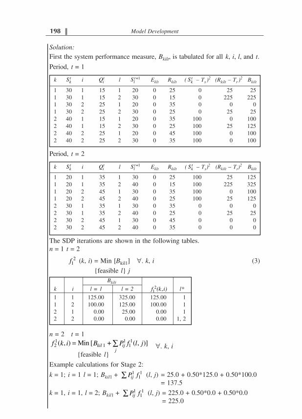
��� Model Development
Solution:
First the system performance measure, Bkilt, is tabulated for all k, i, l, and t.
Period, t = 1
k tkS i t
iQ l +1tlS Eklt Rkilt ( t
kS – Ts )2 (Rkilt – Tr )2 Bkilt
1 30 1 15 1 20 0 25 0 25 25
1 30 1 15 2 30 0 15 0 225 225
1 30 2 25 1 20 0 35 0 0 0
1 30 2 25 2 30 0 25 0 25 25
2 40 1 15 1 20 0 35 100 0 100
2 40 1 15 2 30 0 25 100 25 125
2 40 2 25 1 20 0 45 100 0 100
2 40 2 25 2 30 0 35 100 0 100
Period, t = 2
k tkS i t
iQ l +1tlS Eklt Rkilt ( t
kS – Ts)2 (Rkilt – Tr)
2 Bkilt
1 20 1 35 1 30 0 25 100 25 125
1 20 1 35 2 40 0 15 100 225 325
1 20 2 45 1 30 0 35 100 0 100
1 20 2 45 2 40 0 25 100 25 125
2 30 1 35 1 30 0 35 0 0 0
2 30 1 35 2 40 0 25 0 25 25
2 30 2 45 1 30 0 45 0 0 0
2 30 2 45 2 40 0 35 0 0 0
The SDP iterations are shown in the following tables.
n = 1 t = 2
21f (k, i) = Min [Bkil1] �� k, i (3)
{feasible l} j
Bkilt
k i l = 1 l = 2 21 ,f (k i) l*
1 1 125.00 325.00 125.00 1
1 2 100.00 125.00 100.00 1
2 1 0.00 25.00 0.00 1
2 2 0.00 0.00 0.00 1, 2
n = 2 t = 11 1 12 1 1( , ) = Min [ + ( , )] kil ij
j
f k i B P f l j� �� k, i
{feasible l}
Example calculations for Stage 2:
k = 1; i = 1 l = 1; Bkil1 + 1 11ijP f� (l, j) = 25.0 + 0.50*125.0 + 0.50*100.0
= 137.5
k = 1, i = 1, l = 2; Bkil1 + 1 11ijP f� (l, j) = 225.0 + 0.50*0.0 + 0.50*0.0
= 225.0

Reservoir Systems—Random Inflow ���
k = 1, i = 2, l = 1; Bkil1 + 1 11ijP f� (l, j) = 0.00 + 0.30*125.0 + 0.70*100.0
= 107.5
k = 1, i = 2, l = 2; Bkil1 + 1 11ijP f� (l, j) = 25.00 + 0.30*0.0 + 0.70*0.0
= 25.0
k = 2, i = 1, l = 1; Bkil1 + 1 11ijP f� (l, j)
= 100.00 + 0.50*125.00 + 0.50*100.00
= 212.5
Bkil1 + 1 11ijP f� (l, j) 1
2f (k, i)
K i l = 1 l = 2 l*
1 1 137.50 225.00 137.50 1
1 2 107.50 25.00 25.00 2
2 1 212.50 125.00 125.00 2
2 2 207.50 100.00 100.00 2
n = 3 t = 2
23f (k, i) = Min [Bkil2 + 1 1
2ijj
P f� (l, j)] � k, i
{feasible l}
Bkil2 + 1 12ijP f� (i,j) 2
3f (k, i)
k i l = 1 l = 2 I*
1 1 195.00 435.00 195.00 1
1 2 215.00 245.00 215.00 1
2 1 70.00 135.00 70.00 1
2 2 115.00 120.00 115.00 1
n = 4 t = 1
14f (k,i) = Min [Bkil1 + 2 2
3ijj
P f� (l,j)] �k,i
{feasible l}
Bkil1 + 2 23ijP f� (l, j) 1
4f (k,l)
k i l = 1 l = 2 I*
1 1 230.00 317.50 230.00 1
1 2 209.00 126.50 126.50 2
2 1 305.00 217.50 217.50 2
2 2 309.00 201.50 201.50 2
Proceeding in a similar manner, further computations are shown as follows:
n = 5 t = 2
k i l:1 l:2 25f (k, i) l*
1 1 292.90 532.90 292.90 1
1 2 309.30 339.30 309.30 1
2 1 167.90 232.90 167.90 1
2 2 209.30 214.30 209.30 1

��� Model Development
n = 6 t = 1
k i l:1 l:2 16f (k, i) l*
1 1 326.10 413.60 326.10 1
1 2 304.38 221.88 221.88 2
2 1 401.10 313.60 313.60 2
2 2 404.38 296.88 296.88 2
n = 7 t = 2
k i l:1 l:2 27f (k, i) l*
1 1 388.57 628.57 388.57 1
1 2 405.26 435.26 405.26 1
2 1 263.57 328.57 263.57 1
2 2 305.26 310.26 305.26 1
n = 8 t = 1
k i l:1 l:2 18`f (k,i) l*
1 1 421.91 509.41 421.91 1
1 2 400.25 317.75 317.75 2
2 1 496.91 409.41 409.41 2
2 2 500.25 392.75 392.75 2
The computations are terminated after this stage because it is verified that
the annual system performance measure remains constant, (being nearly 96).
The steady state policy is tabulated as follows:
Steady state policy for period 1
k i l*
1 1 1
1 2 2
2 1 2
2 2 2
Steady state policy for period 2
k i l*
1 1 1
1 2 1
2 1 1
2 2 1
Verify that the expected annual system performance measure [ +t
n Tf (k, i) –t
nf (k, i)] remains constant for all k, i, and t once the steady state is reached.
In this example the expected annual performance is approximately 96 units
(e.g. 18f (1, 1) – 1
6f (1, 1) = 421.91 – 326.10 = 95.81).

Reservoir Systems—Random Inflow ���
�� !"#$����� The steady state policy for a two-period problem is specified
as follows:
t = 1 t = 2
k i l* k i l*
1 1 1 1 1 1
1 2 2 1 2 1
2 1 2 2 1 1
2 2 2 2 2 2
The inflow transition probabilities are as given in the following table.
t = 2 t = 1
j j
t=1 i 1 2 t = 2 i 1 2
1 0.5 0.5 1 0.4 0.6
2 0.3 0.7 2 0.8 0.2
Obtain the steady state probabilities of release, inflow, and storage.
Solution:
Computation of PRkit
Solving the following simultaneous equations will yield the values of PRkit.
+1 = * tljt kit ij
k i
PR PR P�� � l, j, t.
l = l(k, i, t)
kitk i
PR�� = 1 � t
t = 1:
PR112 = 111PR * 0.5;
PR122 = 111PR * 0.5;
PR212 = 121 *PR 0.3 + 211 *PR 0.5 + 221 *PR 0.3;
[Note that l = 2 in period t = 1 results from three combinations of (k, i), viz.,
(1, 2), (2, 1) and (2, 2). Hence the three terms in summation]
PR222 = 121 *PR 0.7 + 211 *PR 0.5 + 221 *PR 0.7; (A)
t = 2:
PR111 = 112 *PR 0.4 + 122 *PR 0.8 + 212 *PR 0.4;
PR121 = 112 *PR 0.6 + 122 *PR 0.2 + 212 *PR 0.6;
PR211 = 222 *PR 0.8;
PR221 = 222 *PR 0.2; (B)
Additionally,
PR111 + PR121 + PR211 + PR221 = 1;
PR112 + PR122 + PR212 + PR222 = 1; (C)

��� Model Development
There is a total of 8 probabilities, PRkit
Taking any three of equations (A) for t = 1, any three equations (B) for
t = 2, and the last two equations (C) (one for each period t), the set of 8
equations are solved for 8 values of PRkit. The resulting PRkit values are
shown in the following table.
k i PRkit k i PRkit
1 1 0.284 1 1 0.142
t = 1 1 2 0.284 t = 2 1 2 0.142
2 1 0.346 2 1 0.284
2 2 0.086 2 2 0.432
Steady state probabilities of storage and inflow:
Storage:i
=kt kitPS PR� � k,t
t = 1
PS11 = PR111 + PR121
= 0.284 + 0.284
= 0.568
PS21 = PR211 + PR221
= 0.346 + 0.086
= 0.432
t = 2
PS12 = PR112 + PR122
= 0.142 + 0.142
= 0.284
PS22 = PR212 + PR222
= 0.284 + 0.432
= 0.716
Inflow: =it kitk
PQ PR� � i, t
t = 1
PQ11 = PR111 + PR211
= 0.284 + 0.346
= 0.63
PQ21 = PR121 + PR221
= 0.284 + 0.086
= 0.37
t = 2
PQ12 = PR112 + PR212
= 0.142 + 0.284
= 0.426
PQ22 = PR122 + PR222
= 0.142 + 0.432
= 0.574

Reservoir Systems—Random Inflow ���
Problems
6.4.1 Solve the two-state, two-period SDP reservoir operation problem with
the following data to obtain steady state release policy.
Transition Probabilities
Period t = 1l t
iQ k tkS
1 15 1 30
2 25 2 40
Period t = 2I t
iQ k tkS
1 35 1 20
2 45 2 30
Reservoir capacity = 60 units
Bkilt = | Rkilt – TR | + | tkS – Ts |
with TR = 55; Ts = 30
6.4.2 The steady state release probabilities obtained from an SDP solution
are given below, with notations followed in the text.
k i PRkit
t = 1 t = 2
1 1 0.112 0.320
1 2 0.053 0.115
2 1 0.144 0.166
2 2 0.532 0.200
3 1 0.080 0.090
3 2 0.079 0.109
Obtain the steady state probabilities of inflows and storages.
6.4.3 The following inflow transition probabilities are given for a two-state,
two-period SDP reservoir operation problem.
t = 2 t = 1
0.9 0.1 0.4 0.6
t = 1 t = 2
0.5 0.5 0.2 0.8
The steady state policy obtained from the SDP solution is as given
below:
t = 1 t = 2
k i l* k i l*
1 1 1 1 1 2
1 2 1 1 2 2
2 1 2 2 1 2
2 2 1 2 2 1
Obtain the steady state probabilities for release, storage, and inflows
from this solution.
j t = 2 j t = 1
i 1 2 i 1 2
1 0.5 0.5 1 0.4 0.6
2 0.3 0.7 2 0.8 0.2
t = 1 t = 2

��� Model Development
������&���
1. Chow, V.T., D.R. Maidment, and L.W. Mays, Applied Hydrology, McGraw-
Hill Book Co. New York, 1988.
2. Haan, C.T., Statistical Methods in Hydrology, Iowa State University Press,
Ames, 1977.
3. Nayak, S.C. and Arora “Optimal Capacities for a Multireservoir System
using the Linear Decision Rule”, Water Resources Research, Vol. 7, No.
3, 1971.
1. Datta, Bithin and S.D. Dhiman, “Chance Constrained Optimal Monitoring
Network Design for Pollutants in Groundwater”, Journal of Water Re-
sources Planning and Management, ASCE, May–June, 1996.
2. Datta, Bithin and Mark H. Houck, “A Stochastic Optimization Model for
Real-Time Operation of Reservoirs Incorporating Forecast Errors”, Water
Resources Research, 20(8), 1984.
3. Datta, Bithin and Stephen J. Burges, “Short-term Single, Multi-purpose
Reservoir Operation: Importance of Loss Functions and Forecast Errors”,
Water Resources Research, 20(9), 1984.
4. Houck, Mark H. and Bithin Datta, “Performance Evaluation of a Stochas-
tic Optimization Model for Reservoir Design and Management with Ex-
plicit Reliability Criteria”, Water Resources Research, 17(4), 1981.
5. Loucks, D.P. and P. Dorfman, “An Evaluation of Some Linear Decision
Rules in Chance Constrained Models for Reservoir Planning and Opera-
tion”, Water Resources Research, 11(6), 1970.
6. Loucks, D.P., J.R. Stedinger, and D.A. Haith, Water Resource Systems
Planning and Analysis, Prentice Hall, Inc, Englewood Cliffs, N.J., 1981.
7. Mays, L.W. and Y.K. Tung, Hydrosystems Engineering and Management,
McGraw Hill, Inc., New York, 1992.
8. Mujumdar, P.P., and Sandeep Narulkar, “Optimization Models for
Multireservoir Planning and Operation”, Jal Vigyan Sameeksha, Vol. VIII,
No. 1 pp. 29–52, 1993.
9. Ossenbruggen, P.J., Systems Analysis for Civil Engineers, John Wiley and
Sons, New York, 1984.
10. Simonovic, S.P. and M.A. Marino, “Reliability Programming in Reservoir
Management, 3: System Of Multipurpose Reservoirs”, Water Resources
Research, 18(4), 735–743, 1982.
11. Trezos, T., and W.W.G. Yeh, “Use of Stochastic Dynamic Programming
for Reservoir Management”, Water Resources Research, 23(6), 983–996,
1987.
12. Yeh, W.W.G., “Reservoir Management and Operations Models: A State-
of-the-Art Review”, Water Resources Research, 21(12), pp. 1797–1818,
1985.

���� �
����������
� Applications of Linear Programming
� Applications of Dynamic Programming
� Recent Modelling Tools

������� �
�������������� ��������������
n this chapter we discuss some applications of linear programming to water
resources problems, with a specific focus on irrigation.
��� ������������ ����������������� ���������� �����
Most problems dealing with planning for irrigation schedules involve alloca-
tion of a known quantity of water across intraseasonal time periods, consisting
typically of one week to ten days. Such problems may be posed as optimization
problems and, with suitable simplifications, may be formulated as linear pro-
gramming (LP) problems. In this section, we discuss such formulations, and
provide indicative results of example applications. The concept of crop yield
optimization is first discussed as a prerequisite for understanding the material
covered subsequently in the chapter.
����� ���������������� !���"
The objective of an irrigation water management problem is to maximize a
measure of crop production, taking into account the response of the crop to the
amount of irrigation applied. To achieve this through a mathematical program-
ming technique, crop production functions are normally used. Typical crop
production functions (see, Doorenbos and Kassam, 1979 and Sarma, 2002 for a
detailed discussion on crop production functions) relate the yield ratio (ratio of
actual to maximum yield) of a crop to a function of the evapotranspiration ratio
(ratio of actual to potential evapotranspiration) over the growth stages. At
present, a single crop production function that is applicable to all crops, grow-
ing seasons, and climates is not available. We use here a simple additive form
of production function to discuss formulation of the optimization problems.
This is of the form
I

#$% Applications
� �1
= 1 1Ng
ggm g
y AETKy
y PET�
� �� � � �� �� �� � � � (7.1)
where Ng is the number of growth stages in the crop season.
g is the growth stage index
Kyg is the yield factor for the growth stage g
y is the actual yield of the crop
ymax is the maximum yield of the crop
AET is the actual evapotranspiration, and
PET is the potential evapotranspiration
The yield factor, Kyg, indicates the sensitivity of the crop yield to the evapo-
transpiration deficit in growth stage g. The soil moisture balance, which forms
an important constraint in the optimization problems for irrigation water
allocation, is schematically shown in Fig. 7.1, and is written for a crop c as
+1 +1 +10= ( )t t t t t t t t t t
c c c c c c c c cD D RAIN q AET D D DP� � � � � � (7.2)
where tc� is the soil moisture of crop c at the beginning of the period t, t
cD is
the root depth of crop c during period t, RAINt is the effective rainfall (contri-
bution of rainfall to soil moisture) in the command area in period t, tcq is the
irrigation application to crop c in period t, AETtc is the actual evapotranspira-
tion of crop c in period t, �0 is the initial soil moisture in the soil zone into
which the crop root extends at the beginning of period t + 1, and tcDP is the
deep percolation. The soil moisture values tc� and �0 are in units of depth per
unit root depth and all other terms are in depth units.
The relationship between AET/PET ratio and the available soil moisture is
approximated by a linear relationship, with AET = 0, when the available soil
moisture is zero (corresponding to the actual soil moisture at wilting point) and
AET = PET when the available soil moisture is equal to the maximum available
soil moisture (corresponding to the actual soil moisture at field capacity). �f ,
and �w are soil moistures at field capacity and wilting point, respectively, in
depth per unit depth (of root zone) units. For use in linear models, the AET
constraint is written as
Period + 1t
Period t
t tcRAIN q t
cAET
tcD�t t
c cD
tcDP
� 1 1t tc cD
� �10( )t t
c cD D
1tcD
��&����� ��������������� ���������������������

Applications of Linear Programming #$'
( )
( )
t t t t tc c c w ct t
c ctf w c
D RAIN q DAET PET
D
� �
� �
�� �
�(7.3)
tcAET � t
cPET (7.4)
Consider the problem of allocation of a known amount of water available
for the entire season among different intraseasonal periods of a crop. This
problem may be formulated as an LP problem as follows:
Max 1
tTt
tt
AETKy
PET�
�� �� �
Subject to � t+1 = � t + q t + RAIN t – AET t – DP t �t
AET t � (� t + q t + RAIN t – �w) �( )
t
f w
PET
� ���t
AET t � PET t �t
� t+1 � �f � � t �t
DP t � M � � t �t
�w � � t+1 � �f �t
1
Tt
t
q� A � Q
with nonnegativity of all decision variables. � is a binary integer variable and
M is a large number, both introduced to ensure that the deep percolation is
nonzero only when the soil moisture is at field capacity. Q is the known
amount of water (volume) available for the entire season, and qt is the amount
of water (depth) allocated in period t, A is the crop area. The problem is
formulated for a constant root depth so that the soil moistures �, �f and �w in
the above formulation are in depth units.
(!���������� Consider the following data for a single crop:
Crop type: two seasonal (such as cotton grown in many parts of South India)
Crop period: 6 months (18 intraseasonal time periods of 10 days each)
Crop area: 3902.50 hectares
Field capacity: 33.2% (3.32 mm/cm)
Wilting point: 16.5% (1.65 mm/cm)
Root Depth of the crop: 100 cm (assumed to be constant)
Rainfall Data
Time
periods 1 2 3 4 5 6 7 8 9 10 11 12 13 14 15 16 17 18
(10 days)
Rainfall
(Raint) 0.5 0.0 0.0 120.0 2.0 2.0 0.0 1.0 0.0 0.0 0.0 1.0 150.0 7.0 3.0 0.0 6.7 0.0
in mm

#�$ Applications
��&����# ��������������������� ��� ������������ �
�������� !�����
Time
periods
(10 days) 1 2 3 4 5 6 7 8 9 10
PET (mm) 12.32 9.49 11.68 19.06 17.59 35.35 22.20 30.65 37.22 40.65
Ky 0.20 0.20 0.20 0.25 0.25 0.25 0.25 0.25 0.25 0.25
Time
periods
(10 days) 11 12 13 14 15 16 17 18
PET (mm) 42.19 35.06 36.01 37.42 47.72 45.58 40.4 44.04
Ky 0.25 0.25 0.25 0.25 0.25 0.25 0.25 0.25
Initial soil moisture is assumed to be just above the wilting point.
When the LP problem is solved for various levels of available water, Q, the
resulting allocations, variations of AET, and the soil moistures will be as
shown in Figs. 7.2 to 7.4. The crop yield ratio (ratio of crop yield to maxi-
mum crop yield) resulting from the optimal allocations are given in Table 7.1.
Such analyses are useful in irrigation scheduling of a known seasonal amount
of available water.

Applications of Linear Programming #��
�!)������ !��������� "����#����$���������� ������%��&����'�(
Sl No. Q (Mm3) Yield Ratio*
1 30 1.000
2 25 1.000
3 20 0.823
4 15 0.465
5 10 0.085
6 5 0.0
*yield ratio = y/ym (see Eq. 7.1).
��&����* !��������� ���!����� ��� ������������ �
��&����+ !��������� ������������ ��� ������������ �
0
50
100
150
200
250
300
350
0 2 4 6 8 10 12 14 16 18 20
Time periods (in 10 days)
Soil moisture at 30 Mcum
Soil moisture at 25 Mcum
Soil moisture at 20 Mcum
Soil moisture at 15 Mcum
Soil moisture at 10 Mcum
Soil moisture at 5 Mcum
So
ilm
ois
ture
(in
mm
)

#�# Applications
����# ����&!���"��!��������,!���"�����-�����������.
Consider the problem of water allocation in canal command areas, in which a
known amount of water, Qt , t = 1, 2,… T is to be allocated to multiple crops in
periods across their growing seasons. The LP model already discussed for
single crop allocation may be modified as follows, with c indicating a crop, and
t a time period:
Max 1 1
tN Tct
c tc t c
AETKy
PET� �
�� �� �
Subject to +1=t t t t t tc c c c cq RAIN AET DP� � � � �c, t
( )( )
tct t t t
c c c c wf w
PETAET q RAIN� �
� �� � �
��c, t
t tc cAET PET� �c, t
+1t tc f c� � �� � �c, t
tcDP � M � t
c� �c, t
�w � +1,tc� � �f �c, t
1
Ntc
c
q� � Qt �t
The notations used have the same meaning as before, with the subscript c
denoting crop c. N is the number of crops.
(!����� ����# Consider an allocation problem for three crops. The crop
calendar, available irrigation water, and rainfall in the command area are
given in Fig. 7.5 and Table 7.2, for a season consisting of 18 ten-day periods.
The crop areas are 3902.50 ha (cotton), 1977.43 ha (jowar) and 33.10 ha
(groundnut). The PET values for these crops are computed from pan evapora-
tion data (not given here). The problem is to allocate the known amount of
water Qt, in period t, to the three crops, such that the total (relative) crop yield
is maximized at the end of the season. Note that the amount of water available
in a period is a deterministic value, known in advance for all periods t.
��&����/ )��*)�������

Applications of Linear Programming #�*
The field capacity is 33.20% and wilting point is 16.50%. The root depth is
assumed to be 100 cm throughout the season for all crops. The problem is
analyzed for various levels of available irrigation water with the available
amount of water given in Table 7.2, taken as the maximum amount Q.
Figures 7.6 to 7.8 show variations of allocations to the three crops with
various levels of available water.
�!)�����# #��� ������������%��������������**��
Time
periods
(10 days) 1 2 3 4 5 6 7 8 9 10
Rainfall
(Raint) (mm) 0.5 0.0 0.0 120.0 2.0 2.0 0.0 1.0 0.0 0.0
Available
irrigation
supply
(Qt) Mcum 3.65 3.65 3.65 5.70 3.70 3.50 3.20 3.20 3.50 3.50
Time
periods
(10 days) 11 12 13 14 15 16 17 18
Rainfall
(Raint) (mm) 0.0 1.0 150.0 7.0 3.0 0.0 6.7 0.0
Available
irrigation
supply
(Qt) Mcum 3.70 3.70 5.80 5.60 4.00 4.00 5.00 3.00
��&����0 !��������� &��������������$���&����������%�����'�( ��)�����

#�+ Applications
��&����� !��������� &��������������&���&����������%�����'�( ��+�$��
��&����% !��������� &��������������$���&����������%�����'�( ��,��������

Applications of Linear Programming #�/
Allocations obtained from the LP model account for competition among
crops for water through the crop sensitivity factors Kyct. The optimal alloca-
tions in a period depend on a number of factors such as water available, time
of season, soil moistures of individual crops in the period, potential
evapotranspiration of the crops, rainfall in the period, and crop areas. Note
that in this example, the water available in intraseasonal periods across the
crop season is assumed to be known. In planning reservoir releases for
irrigation, however, the water available for irrigation itself becomes a deci-
sion variable, along with cropwater allocations, as shown in Secs. 7.3 and 7.4.
��# ������ � �1������� �������������������
A river basin is considered for expanding its irrigation operations in its rela-
tively less developed upper basin, without detriment to the irrigation needs of
the lower basin, which is fully developed.
A four-reservoir system in the upper basin is considered for development
with given reservoir capacities. The crops proposed to be grown and the land
area available for cultivation in the command area of each reservoir are given.
Irrigation requirements of each crop per unit area are worked out at each site
and are known.
The four-reservoir system comprising the upper basin is modelled with
monthly time periods by using LP to determine the crops to be irrigated and the
extent of irrigation at each reservoir subject to land, water, and downstream
release constraints. Under conditions of limited water supply, there are two
options of irrigation considered: one is to provide intensive irrigation to those
crops that yield higher economic returns (these are also the crops that need
relatively more water) and leave the others unirrigated; the other is to allocate
the available water to crops over a wider area to provide extensive irrigation.
Accordingly, two objectives are studied: one of maximizing the net economic
benefits (from both irrigated as well as unirrigated cropped areas at all reservoirs)
and the other of maximizing the total irrigated cropped area at all the reservoirs
in the upper basin. These two conflicting objectives are studied for analyzing
the tradeoff between them from the point of view of multiobjective planning,
using the constraint method (Section 4.2.2).
The model decides the crops to be irrigated and the extent of irrigation. If a
crop is considered at all for irrigation, under either option mentioned above, it
receives its full water requirements in all periods of the crop season.
The four-reservoir system in the upper basin is shown in Fig. 7.9. There are
two reservoirs B and D on the main river, and the other two, A and C, on the
tributaries. There is existing irrigation at reservoirs B and D. Expansion of
irrigation at B and new cropped areas at A and C are proposed.

#�0 Applications
The reservoir capacities and land area proposed for irrigation are as shown
in Table 7.3.
�!)�����* #��������)�*���������������
J Reservoir Drainage area, Capacity, Land area proposed
km2 Mm3 for irrigation, ha
1 A 5200 962.77 248,900
2 B 9666 1,268.59 77,900*
3 C 6693 453.07 87,800
4 D 19993 2467.60 …
*This is in addition to the existing irrigation at Reservoir B.
���������
A linear programming model is formulated with monthly time periods to deter-
mine the crops and crop areas to be irrigated at each of the sites A, B, and C,
subject to minimum downstream releases from reservoir D to meet the existing
irrigation requirement in the lower basin. The model considers the option of
irrigating or not irrigating any or all of the cropped area under each crop, for
each objective.
Objective 1 Maximize the total net economic benefits from all crops in the
upper basin.
The objective function is written as
3 3
1 1 1 1
maxj jM M
ij ij ij ijj i j i
I U� �� � � �
�ij net benefits at site j per unit area of irrigated crop i ( j = 1, reservoir A;
j = 2, reservoir B; and j = 3, reservoir C);
�ij net benefits at site j per unit area of unirrigated crop i;
Iij irrigated area at site j under crop i;
Uij unirrigated area at site j under crop i; and
Mj total number of crops considered at site j.
��&����' ���������������� ���#�������������������

Applications of Linear Programming #��
Objective 2 Maximize total irrigated area from all crops in the upper basin.
3
1 1
maxjM
ijj i
I� �
��� ����
Land Allocation Constraints The same land should be made available for a
given crop throughout the growing season.
For all the growing months m of crop i at site j
Iijm = Iij for all m,
where Iijm is the irrigated area at site j under crop i in period m.
For all the growing months m of crop i at site j,
Uijm = Uij for all m,
where Uijm is the unirrigated area at site j under crop i in period m.
Storage—Continuity Equations The equations for the four sites j = 1, 2, 3, 4
are written as follows:
These constraints are valid for all time periods, m = 1, 2, …, 12.
For j = 1
1
1 1 1 1 1 1 1 11
M
m m i m i m m m mi
S S p I R E F�
� � � � �
For j = 2
2
2 2 1 1 2 2 2 2 2 21
M
m m m i m i m m m m mi
S S R p I R E F W�
� � � � �
For j = 3
3
3 3 1 3 3 3 3 31
M
m m i m i m m m mi
S S p I R E F�
� � � � �
For j = 4
4 4 1 2 3 4 4 4 4m m m m m m m mS S R R R E F W� � � �
where
Sjm storage at site j at the beginning of month m;
pijm water diversion requirement of crop i (in depth units) at j during its
growing month m, and equal to zero for the nongrowing months;
Rjm d/s release from the reservoir at site j during the month m;
Ejm Reservoir evaporation at site j during the month m;
Fjm mean inflow (unregulated) at site j during month m; and
Wjm water diversion requirement at site j for all existing crops during month
m (this term will appear only for j = 2, and for j = 4, as per existing
irrigation requirements. Additional irrigation to ten proposed crops, i, at
site j = 2 is considered)

#�% Applications
Land Area Constraints The total cropped area (irrigated and/or unirrigated)
in each month is less than the possible maximum at each site.
1
( ) 1, 2, 3 1, 2, ,12j
M
ijm ijm ji
I U L j m�
� � � �
where Lj = land available under the command of the reservoir at site j.
For a given crop calendar, the total number of governing constraints at each
site may be less than 12 because some constraints may be repetitive or may
form a subset of other constraints. In a month where one crop ends and another
begins, the area of the crop ending in that month is not included in the con-
straint to permit the possible use of the land for both crops in that month.
Downstream Release Constraints The release from the reservoir at site 4,
R4m, should be greater than the minimum downstream release specified by
(DR)m, which is arrived at on the basis of the requirements for existing irriga-
tion below reservoir D. Then
R4m � (DR)m � m
Capacity Constraints The storage in each reservoir is limited to its capacity
(live storage) at all times.
Sjm � Sjmax ��� j, mwhere Sjmax is the live storage capacity of the reservoir at site j.
����������
The first month (m = 1) corresponds to June as per the water year in India
(June 1 to May 31). Twelve principal crops are proposed to be grown in the
command area of reservoir A, 10 crops in the command area of reservoir B, and
14 in the command area of reservoir C. Crop water requirements are estimated
as per standard procedures. Estimated net benefit from irrigated and unirrigated
crops per unit area (Table 7.4), and release requirements downstream of
Reservoir D (based on the existing cropping in the lower basin, as given in
Table 7.5) are the other inputs used in the model.
�!)�����+ ���������-������ ��� )��*�./#�0��
Crop Irrigated Unirrigated
Rice 2950 1525
Ragi/Jowar 2450 1450
Maize 2300 1300
Groundnut 2400 1100
Potato 2500 2380
Wheat 1900 825
Soyabeans 2800 1300
Pulses/Vegetables 600 360
Safflower 375 225
*Obtained by deducting estimated cost of fertilizer from produce value at wholesale prices.

Applications of Linear Programming #�'
�!)�����/ ��������$�������#������#�1�����������#��������'��2(
Month Release Month Release
June 570.0 Dec. 0
July 1668.5 Jan. 329.2
Aug 1360.8 Feb. 569.5
Sept. 775.9 Mar. 708.6
Oct. 0 Apr. 140.0
Nov. 0 May 0
�������
Objective 1 Maximization of net economic benefits (annual): The optimal
cropping for this case is shown in Table 7.6. The table shows what crops are to
be grown, whether they should be irrigated or not, to what extent they should
be grown in each of the areas, and the growing seasons. The maximized net
benefits and the corresponding values of the total diversion and the irrigated
cropped area in the upper basin are also given in the table.
�!)�����0 �������� ����3����-������ ���
Crop Season I/U* Cropped Area, 100 ha
Reservoir A
Rice Jun–Nov I 1244.5
Ragi/Jowar Jun– Oct I 1244.5
Soyabeans Nov– Feb I 557.7
Potato Dec–Mar U 1931.3
Reservoir B
Mulberry Perennial I 207.0
Rice Jun–Nov I 572.0
Soyabeans Nov–Feb I 572.0
Reservoir C
Rice Jun–Nov I 878.0
Potato Nov–Feb U 878.0
Maximum net benefits = Rs. 2084.709 million; total irrigated cropped area = 527,570 ha.
(exclusive of fixed mulberry crop area of 20,700 ha.)*I = irrigated, U = unirrigated.
Objective 2 Maximization of irrigated cropped area (ICA): The solution
obtained for this case is given in Table 7.7.
The maximum net benefits (Objective 1) are Rs 2084.7 million and the
corresponding irrigated area is 527,520 ha. The maximum irrigated cropped
area (Objective 2) is 755,600 ha, an increase of 43%, and the corresponding
net benefits are Rs 1659.6 million, a reduction of 20% when compared to the
results of maximizing Objective 1. In this case, increase in the cropped area
was made possible by replacing the rice and soyabean (November–February)
crops with less water-requiring crops such as ragi, jowar, wheat, vegetables,
and pulses. When the irrigated cropped area is maximized, the model chooses

##$ Applications
�!)������ �������� ����3�������������)��**������'�)�(
Crop Season I/U* Cropped Area, 100 ha
Reservoir A
Rice Jun–Nov I 264.5
Maize Jun–Oct I 492.1
Groundnut Jun–Oct I 1732.4
Wheat Oct–Feb I 1960.0
Potato Dec–Mar U 529.0
Reservoir B
Mulberry Perennial I 207.0
Groundnut Jun–Nov I 572.0
Pulses/Vegetables Nov–Feb I 108.7
Soyabeans Nov–Feb I 463.3
Reservoir C
Rice Jun–Nov I 260.6
Ragi/Jowar Jun–Oct I 617.4
Vegetables and Nov–Mar I 878.0
minor crops
Maximum irrigated cropped area = 755,600 ha; total net benefits = Rs. 1659.623 million
(excluding mulberry over a fixed area of 20,700 ha). *I = irrigated, U = unirrigated,
crops needing relatively lower water requirement, as the total amount of water
available is limited. These are also the crops that yield lower economic
benefits.
Summary of Results
Variable maximized Net Benefits Irrigated Cropped Area (ICA)
Net benefits (106 Rs 1970–72) 2084.709* 5275.700
Irrigated cropped area (100 ha) 1659.623 7556.00*
(*maximum value)
A Multiobjective Approach As the two objectives are conflicting with each
other, multiobjective analysis deals with finding the tradeoff between net in-
come and irrigated cropped area at different levels of development. Figure 7.10
shows the efficiency frontier or the transformation curve for these outputs.
Each of the plotted points in the figure is obtained by maximizing the net
benefits for a fixed value of the irrigated cropped area, using constraint ap-
proach (Section 4.2.2), and corresponds to a plan of cropping such as the one
given in Table 7.6. Any point on the curve defined by these points is Pareto
admissible.
Implicit Tradeoff A total irrigated cropped area of 576,800 ha. (at reservoirs
A, B, and C) is projected for development by the concerned planning agency,
based on rainfall distribution and local conditions. It is interesting to see that

Applications of Linear Programming ##�
the proposed area lies within the range of values obtained for the two objec-
tives (between 527,570 and 755,600 ha.). A chance constrained form of the
model may be used to determine the results for inflows at a specified reliability
level, though the study reported herein does not attempt it.
A tradeoff between the net benefits and the irrigated cropped area can be
found from the curve above (Fig. 7.10) by determining the slope of the curve at
a given value of the irrigated area. For the projected level of 576,800 ha., the
tradeoff works out to Rs 360 per ha. This means that the amount of net benefits
foregone for an increase in the irrigated cropped area (at the level of projection)
is Rs. 360 per hectare, subject to the assumptions and limitations of the model.
For details of the study, refer to Vedula and Rogers (1981).
��* � ���2������������������� ����������������������
In this application, the formulation runs along similar lines to the problem
discussed in Section 6.3.1, except that in the present case we discuss how the
reservoir capacity tradeoff with reliability can be arrived at in the case of
multiple crops, taking into account the soil moisture balance in the root zone of
individual crops (as against lumped demands considered earlier).
A single reservoir is considered for multicrop irrigation. Data on crops,
soils, and potential evapotraspiration of each crop are known, A reliability-
based reservoir-irrigation model is formulated to determine (i) minimum size of
the reservoir needed to meet crop irrigation requirements at a specified level of
reliability, and (ii) maximum reliability of meeting irrigation requirements as-
sociated with a given reservoir capacity, using chance constrained linear pro-
gramming. Reservoir inflow is considered random, and rainfall in the com-
mand area is considered deterministic. The model takes into account water
allocation to multiple crops, soil moisture balance in the root zone of the
cropped area, heterogeneous soil types, and crop root growth with time, and
��&�����$ ����� ��������)���� �����4��� ���������������

### Applications
integrates the crop water allocation decisions with release decisions at the
reservoir. The crops and the crop calendar are assumed fixed. Fortnightly irri-
gation decisions are considered within the crop season.
���������
The salient features of model formulation not covered in Section 6.3.1 are
covered in detail here.
Reservoir Release Policy and Storage Continuity The reservoir release policy
in terms of irrigation water allocations to individual crops and the storage
continuity relationships are written as follows.
The reliability constraint (Section 6.3.1) is written here as
Prob1
( )c ct t
c
R x A ��
� �� �� �� � for all t.
where Rt = release from the reservoir in period, t
� = a parameter equal to the ratio of the total crop water allocation at
the plant level to the reservoir release (to account for conveyance
and other losses).ctx = irrigation allocation to crop c in period t, in depth units
Ac = area of crop c, in area units
� = specified reliability level.
����������� ��������
Soil moisture balance equation for a given crop c in period t is expressed as
(following Section 7.1.1),
+1 +1 +1( ) =c c c c c c c c c ct t t t t t t t t tSM D x RAIN FC D D PET DP SM D � � �
where ctSM is the soil moisture at the beginning of the period t for crop c in
depth units per unit root depth, ctD is the average root depth during period t for
crop c in depth units, ctx is the irrigation allocation in period t for crop c in
depth units, RAINt is the rainfall in period t in depth units, FCc is the soil
moisture at field capacity of the soil for crop c in depth units per unit root
depth, ctPET is the potential evapotranspiration in period t for crop c in depth
units, and ctDP is the deep percolation in period t for crop c in depth units. In
this equation, all variables are considered deterministic. It is assumed that all of
the rainfall infiltrates into the soil. It is implied in this constraint that ctx is
drawn out of the reservoir release to meet the full requirement of ctPET of the
crop. Values of ctx and release Rt are, however, controlled by the reliability
criterion.
Soil Moisture It is assumed that
(i) in the beginning of (the first period of) the season soil moisture is at at
field capacity for all crops, 1cSM = FC c,
(ii) the soil moisture in the incremental crop root depth at the end of the period
is at field capacity, and

Applications of Linear Programming ##*
(iii) soil moisture is bounded by its value at the wilting point (WPc) and at field
capacity (FCc), WPc �� ctSM � FCc.
Potential Evapotranspiration Estimation of the ctPET for crop c in a particu-
lar period t is based on reference evaporation in period t, (ETo)t, and crop
factor ctk for crop c in period t.
PETt =ctk (ETo)t.
The crop factor is a function of the crop growth stage. Values of kt for all t
in a given growth stage are assumed to be equal to the crop factor for that
growth stage.
Deep Percolation Deep percolation is suitably penalized in the objective
function so that it occurs only when the soil moisture at end of the period is at
field capacity.
���� �����������������
The deterministic equivalent of the reliability constraint is written using a
linear decision rule as in Section 6.3.1.
[(1 + at)bt – (1 – at)bt – 1 + Lt + Dt] � F –1 (1 – �t )
where F –1 (1 – �t) =(1 )ttQ ��
= inflow in period t, with a probability of (1 – �t),
or an exceedance probability of �t.
���� ���� ����
In order to ensure that the soil moisture is brought to field capacity every
period, enabling extraction of water by the plants at their full demand at ctPET
(this assumes that actual evapotranspiration equals PET only when the soil
moisture is at field capacity in the light of the soil moisture balance equation
written earlier), ctx is constrained, as
c c c c ct t t t tSM D x RAIN FC D � for all t.
The total irrigation allocation in any period is to be less than the canal
capacity, CC, in each period.
( )c ct
c
x A � CC for all t.
where CC is the canal capacity given.
����������������
The objective function used is to minimize the active storage capacity K, with a
penalty for deep percolation. Note that this technique of imposing penalty is
different from the formulation in Sec 7.1.1, in which integer variables were
used. Deep percolation will then occur only when it must, i.e. only when the
end-of-period soil moisture is at field capacity. Thus the objective function is
written as
Minimize [K + M ct
t c
DP ]
where M is an arbitrarily large value.

##+ Applications
Application The model is applied to Ghataprabha reservoir in Karnataka to
determine the minimum reservoir capacity for different levels of reliability. The
live capacity of the reservoir is 1389 Mm3. It is assumed that the reservoir
releases water to a composite command comprising the total irrigated area by
the left and right bank canals (which together have a total discharge capacity of
155.95 m3/sec). This is done because of the model’s limitation in dealing with
two different random releases into the two canals (left bank canal and right
bank canal), both of which share the same source of supply (reservoir storage).
Inflow and rainfall data of 35 years are used. Average rainfall in the command
area is computed using Theissen weights.
The crops considered are hybrid maize (95,220 ha) and groundnut
(31,740 ha) in the kharif season; and hybrid maize (63,480 ha), wheat (47,610
ha), and pulses (15,870 ha) in the rabi season. Field capacity of soil is
0.3 cm/cm and the wilting point is 0.1 cm/cm.
�������������
The maximum attainable reliability with existing live capacity of 1389 Mm3 is
determined to be 0.55 or 55%; and the maximum possible reliability, for
the given inflow data, is 80%, for which the minimum required capacity is
1611 Mm3. Reliability higher than this results in an infeasible solution. This
analysis shows that, for the reservoir under study, the maximum attainable
reliability is limited by the existing capacity.
The relationship between reliability and minimum required active reservoir
capacity is plotted in Fig. 7.11. From the curve, the minimum required capacity
for a specified reliability level (within the feasible limit), or the reliability
associated with a given capacity, may be obtained.
��&������ #����%����� )�*����������� )����
The details of the application are given in Vedula and Sreenivasan (1994).
��+ � � �1���� ����������������
Figure 7.12 shows components of a typical surface water irrigation system. In
modelling for integrated reservoir operation, the conveyance system is treated

Applications of Linear Programming ##/
��&�����# )��*������� ��*������� ���&��������������������
as a lumped system and all losses are accounted through a loss term in the
water balance. The irrigation release decisions at the reservoir are to be made
for short time intervals such as a week, ten days or, at the most, two weeks.
Mathematical models which aid decisions over larger time intervals such as a
month or a season are therefore inadequate, as they do not take into account the
variability in irrigation demand within these time intervals. Mathematical mod-
els have therefore been developed to determine a long-term operating policy,
considering the intraseasonal irrigation demands of the crops, and competition
among them in the face of a deficit supply (e.g. Dudley, 1988; Vedula and
Mujumdar, 1992).
��+�� �3�����������.��4�������!���"�5�������&!���"
A short-term reservoir operation typically has an operating horizon of one year.
The problem may be formulated as an LP problem with deterministic inflows.
The inflows are obtained from an appropriate inflow forecasting model, such
as the Auto Regressive Moving Average (ARMA) model. The LP model is
formulated to be solved from the current period tp in real time to the last period
T in the year. The objective is to maximize a measure of crop yield, which may
be expressed as minimization of weighted evapotranspiration deficit.
����������������
1
(1 / )t
p
NTt t t
c c c ct t c
Min P Ky AET PET� �
� (7.4.1)
where tp is the current period in real time, T is the last period in the year, Nt is
the number of crops present in period t, c is the crop index, AETct is the actual
evapotranspiration, PETct is the potential evapotranspiration, Kyc
t is the yield
sensitivity factor of crop c in period t, and Pc is a measure of production for
crop c actually realized up to the beginning of the period t. It may be noted that
as the model is applied in real time, the actual value of the crop production
function up to the beginning of the current period may be quite different from
that predicted when the model was applied in the previous period. The term Pc

##0 Applications
is the value of the second term of the objective function actually realized from
the first period in the year up to the beginning of the current period tp. That is,
1
=1
= (1 / )p
tt t t
c c c ct
P Ky AET PET�
�
Addition of this term in the objective function ensures that at every period,
the allocations are made such that the crop yield in the entire year is maxi-
mized, using the latest available information on the state of the system. In the
dynamic programming model discussed in the next chapter (Sec. 8.3), this
feature is achieved by introducing an additional crop production state variable,
�, for each crop c.
��� ����
Reservoir Storage Continuity The reservoir storage continuity is written, tak-
ing into account the storage-dependent evaporation losses, as
(1 + at)St+1 = (1 – at)St + Qt – Rt – Ot – A0 et t = tp, tp+1,… T (7.4.2)
where at = A0 et /2, A0 is the water spread area corresponding to the dead
storage level, et is the evaporation rate in period t, St is the storage at the
beginning of period t, Qt is the forecasted inflow during period t, Rt is the
release during period t, and Ot is the overflow during period t. Note that while
solving the model the term Ot should be penalized in the objective function to
ensure that it takes nonzero values only when the reservoir storage exceeds the
capacity.
The reservoir storage at the beginning of the current period tp is known.
Stp = S0 (7.4.3)
where S0 is the known live storage of the reservoir at the beginning of the
period. In case of over-year storage, the end condition on the storage also gets
fixed, and an appropriate constraint is included to force the condition that the
storage at the end of the last period T should be at least equal to the specified
over-year storage Soy.
ST+1 � Soy (7.4.4)
Water Available for Irrigation The reservoir release undergoes conveyance,
application, and other losses. The water actually applied for irrigation of crops
must therefore take into account these losses. When a release Rt is made at the
reservoir in a period t, the water available for allocation among crops is given
by
Xt = � Rt t = tp, tp+1, …, T (7.4.5)
where � is the conveyance efficiency accounting for all losses in the release.
Soil Moisture Balance The soil moisture at the beginning of the current
period, tp, is known for all crops. Starting with this known soil moisture, the
soil moistures at the beginning of all subsequent periods up to the end of the
year are computed by the soil moisture continuity, given by
1 1 10 ( )t t t t t t t t t
c c c c t c c c c cD D RAIN x AET D D Dp� � � � � � � �c, t (7.4.6)

Applications of Linear Programming ##�
where tc� is the soil moisture of crop c at the beginning of the period t, Dc
t is
the root depth of crop c during period t, RAINt is the rainfall in the command
area in period t (assuming all rainfall is available to the crop), xct is the irriga-
tion application to crop c in period t, AETct is the actual evapotranspiration of
crop c in period t, �0 is the initial soil moisture in the soil zone into which the
crop root extends at the beginning of period t + 1, and Dpct is the deep
percolation.
The soil moisture �0 is assumed to be known, and in the model application it
is taken to be equal to the field capacity. Sensitivity of the system performance
with variation in �0 is discussed in Mujumdar and Vedula (1992). The soil
moistures �ct, irrigation allocations xc
t, and the actual evapotranspirations AETct
are all decision variables. The relationship between the AET/PET ratio and the
available soil moisture is approximated by a linear relationship, with AET = 0,
when the available soil moisture is zero (corresponding to the actual soil mois-
ture at wilting point) and AET = PET when the available soil moisture is equal
to the maximum available soil moisture (corresponding to the actual soil mois-
ture at field capacity). This condition is written as
AETct
( )
( )
t t t tc c t c w c t
ctf w c
D RAIN x DPET
D
� �
� �
��
��c, t (7.4.7)
and
t tc cAET PET� �c, t (7.4.8)
The constraint (7.4.7) is necessary along with (7.4.8) to restrict the maxi-
mum value of the actual evapotranspiration to the potential evapotranspiration.
The denominator in (7.4.7) is the maximum available soil moisture of crop c in
period t and the term, ( t tc cD� + RAINt + t
cx ) – �wtcD , is the actual available
soil moisture after the addition of rainfall and irrigation application. The crop
root depth in period t is assumed to be known, and in model application an
appropriate root depth model may be used.
Allocation Limit The total water available for irrigation Xt corresponding to
the release Rt must equal the water actually allocated to the crops. That is,
Xt = tc c
C
x A �t (7.4.9)
where Ac is the area of crop c under irrigation. The upper limit on the soil
moisture �ct is the field capacity. Any moisture in excess will go out of the root
zone as deep percolation, which is ensured through the soil moisture balance
equation.
�ct � �f �c, t (7.4.10)
The LP model given by (7.4.1) to (7.4.10) is solved from the current period
tp in real time up to the last period T in the year. The reservoir storage Stp at the
beginning of the period tp, the actual inflow Itp–1 during the previous period
tp –1, and the soil moistures tpc� at the beginning of the period tp for all crops c

##% Applications
are known. Inflow forecasts Qt for the periods starting from the current period
tp to the last period T are obtained by a suitable one-step-ahead-inflow-fore-
casting model (e.g. a model of the Auto Regressive Moving Average, ARMA,
family) that uses the latest available historical inflow, Itp–1. The rainfall inputs
may be provided in a similar way, although in monsoon climates with low
coefficient of variation for rainfall in individual periods, mean rainfall values
may be used as a deterministic input.
The LP model is applied to the case study of the Malaprabha reservoir. For
the case study, water deficit exists mainly in the rabi season, since the kharif
crops are supported to a large extent by the monsoon rains. Table 7.8 gives a
typical output from the model run for the period 16 (first period in the rabi
season). The results presented in the table are obtained by one run of the model
with the current period, Tp, set to 16. The inputs required for this run are the
storage at the beginning of the period, inflow during the previous (i.e. 15th)
period, and the soil moistures of the crops at the beginning of period 16. As
seen from Table 7.8, the two-seasonal crop cotton is already in the advanced
growing season at the beginning of period 16, whereas the other crops are just
at the beginning of the first growth stage. The soil moisture of cotton and the
initial reservoir storage shown in the table are the values obtained by real-time
simulation till the end of the 15th period for the particular year. The soil
moistures of all other crops are assumed to be at field capacity, since the root
depths are very small and, consequently, the amount of water, which is as-
sumed available at the time of sowing, required to keep the root zone at field
capacity is very low. The inflow values shown in the table are all forecasted
inflows from an AR(1) model which uses the actual inflow, 11.32 Mm3 for the
period 15 as an input. In real time, only the release and allocation decisions for
the current period, i.e. period 16, are meant to be implemented. The reservoir
storage and the soil moistures are updated at the end of the period with the
actual values of inflow and rainfall for the optimal release and allocation
decisions.
��/ � � �1���� ��������6����� �������7���
This section presents an application of linear programming formulation for the
operation of a single reservoir for irrigation and hydropower. The purpose of
the model is to maximize hydropower production, subject to satisfying irriga-
tion demands at a specified reliability level. A piecewise linearization tech-
nique for the nonlinear power function is used in this application to enable use
of linear programming as the optimizing tool. Details can be found in Sreenivasan
and Vedula (1996).
The reservoir system consists of a reservoir with irrigation canals (on both
sides of the river) leading to the irrigated area, and a riverbed powerhouse
located at the bed of the river. Water drawn into the canals exclusively for
irrigation incidentally produces a small amount of hydropower in the power-
houses located along the canals. Power is produced out of the water released

#*$ Applications
downstream of the reservoir in the riverbed powerhouse. The hydropower pro-
duced by the riverbed turbines alone is considered for modelling. The model
considers variations in the head over the turbines with the reservoir water level.
Also it produces hydropower only within a range of reservoir water levels as
may be specified. Irrigation demands into both canals are lumped at the canal
head, against which water is withdrawn (irrigation release) from storage. The
irrigation release (into the canals) is considered to be a random variable along
with reservoir inflow.
The model maximizes the hydropower production from the reservoir with a
specified reliability of meeting irrigation demand, using chance constrained
linear programming (CCLP). Figure 7.13 gives a schematic layout of the
reservoir system.
��&�����* #��������������'���������(
���������
Release Policy The reservoir release policy is defined by a chance constraint.
The probability of irrigation release, IRt, in time t equalling or exceeding the
irrigation demand, Dt, is greater than or equal to a specified value, P, where P
is the reliability level of meeting irrigation demand.
Prob [IRt � Dt] � P (7.5.1)
Reservoir Water Balance The reservoir storage continuity is expressed as
St + It – IRt – Rt – EVt = St +1 (7.5.2)
where St is the total storage at the beginning of period t, It is the random inflow
into the reservoir, IRt is the total irrigation release, Rt is the downstream re-
lease, assumed deterministic, for bed power production, and EVt is the evapora-
tion loss during period t.
EVt is approximated by a linear relationship,
EVt = �t + �t (St + St+1) (7.5.3)
where �t and �t are coefficients depending on the period t.
Substituting for evaporation term from Eq. 7.5.3 into Eq. 7.5.2, and
rearranging
IRt = (1 – �t)St – (1 + �t)St +1 + It – Rt – �t (7.5.4)
Substituting Eq. (7.5.4) into chance constraint Eq. (7.5.1), one gets
Pr[(1 + �t)St+1 – (1 – �t)St + Rt + �t + Dt � It] � P (7.5.5)

Applications of Linear Programming #*�
The deterministic equivalent is written using the linear decision rule (LDR)
IRt = St + It – Rt – EVt – bt (7.5.6)
where bt is a deterministic parameter.
As a consequence,
St +1 = bt (7.5.7)
Effectively, storage is made deterministic. EVt and Rt, both being functions
of storage, are deterministic.
Deterministic Equivalent The deterministic equivalent of the chance con-
straint Eq. 7.5.5 is
(1 + �t)bt – (1 – �t)bt –1 + Rt + �t + Dt ��(1 )PtI�
(7.5.8)
where (1 )PtI�
is the reservoir inflow during period t, with probability (1 – P), or
exceedance probability P.
Other Constraints Storage capacity constraints: The storage in any time pe-
riod t should not be less than dead storage capacity (Kd) and should not exceed
the total capacity (including dead storage), KT.
bt–1 � Kd (7.5.9)
bt–1 � KT (7.5.10)
with bo = b12 for a steady state solution.
Power plant capacity: The energy produced by the riverbed turbine in any
time period t, EBt, should not exceed that corresponding to the installed capac-
ity of the turbine, BC; thus
EBt � BC (7.5.11)
Head–Storage Relationship The reservoir water level and the storage are
assumed to be linearly related. The reservoir elevation, Ht, in any period, t, for
this purpose is computed as the average of the elevations at the beginning and
at end of the period. The following linear relationship is assumed within the
range of storages defined by Eqs. 7.5.9 and 7.5.10.
Ht = � [(bt–1 + bt)/2] + � (7.5.12)
where � is the slope of the linear portion of the elevation-storage curve, and � is
the intercept.
The net head acting on the turbine is Ht – BTAIL, where BTAIL is the tail water
level.
��� �!�� �"�������#� �$�%� �$ ��������������
A linear approximation of the nonlinear power production term following Loucks
et al. (1981) is used. The nonlinear power production term, Qt Ht, where Qt is
the flow and Ht is the head, for example, may be linearized by the approxima-
tion
Qt Ht = Qt Hto + Qto Ht – Qto Hto
where Qto and Hto are the average values of Qt and Ht, respectively.
Following this,
EBt = c [Rt (Ht – BTAIL)] is expressed as
EBt = c [Rt (Hto – BTAIL) + Rto (Ht – BTAIL) – Rto (Hto – BTAIL)] (7.5.13)

#*# Applications
where Rto is the approximate value for the bed power release, Rt, in period t,
and Hto is the approximate value for the reservoir elevation, Ht, in period t,
BTAIL is the tail-water elevation of the bed turbine, and c is a constant to
convert the product of the rate of flow and the head over the turbine into
hydropower produced from the turbine.
The operating range of the reservoir elevation for power production is speci-
fied as
Hmin � Ht � Hmax for bed turbine operation, Hmin and Hmax being specified.
Objective Function The objective is to maximize the annual hydropower
production by the bed turbine.
Maximize tt
EB (7.5.14)
Methodology The CCLP model is run for a specified value of P (reliability).
Initially, the solution is obtained by assuming some reasonable values Hto and
Rto for each t. If the values of Ht and Rt in the solution are different from these,
then another run is made, replacing Hto and Rto by Ht and Rt, respectively. Thus
the CCLP model is run successively each time, replacing the values of Rto by
Rt, and Hto by Ht, till convergence is reached, i.e. Ht � Hto and Rt � Rto, within
a specified tolerance limit.
The model is run for increasing values of P, until the solution becomes
infeasible. This gives the maximum reliability possible for the given inflow
data.
The model is applied to Bhadra Reservoir in Karnataka. The total storage
capacity of the reservoir is 2024 Mm3, with a dead storage capacity of
240 Mm3. The installed capacity of the bed turbine is 24,000 kW. Inflow data
of 52 years are used in the study. Each time a run is made for a particular value
of P, the corresponding inflow sequence for the 12 months has to be used.
Table 7.9, for example, gives monthly inflows with P = 0.65, along with
irrigation demands.
�!)�����' �� ��$���56789/�������������������
Month Inflow (Mm3) Irrigation demand (Mm3)
Jun 163.40 119.90
Jul 813.20 136.80
Aug 702.97 200.60
Sep 261.73 195.80
Oct 302.81 203.20
Nov 89.31 189.70
Dec 50.52 109.40
Jan 26.93 137.30
Feb 17.10 180.10
Mar 10.64 197.39
Apr 11.70 197.90
May 11.06 178.60

Applications of Linear Programming #**
The model solution shows that the maximum possible reliability of meeting
irrigation demands is 0.65, or 65%, and the corresponding maximum annual
hydro-energy produced by the bed turbine is 5.68 M kwh.
Figure 7.14 shows a plot of reliability versus annual hydro-energy produced
from the riverbed turbine. The curve gives the energy that can be produced at
other levels of reliability.
��&�����+ ����������������������#����%����������
From the curve, one can find the maximum annual energy that can be
produced by the bed turbine for a specified reliability of meeting irrigation
demands; or, alternatively, one may find the reliability of meeting irrigation
demands at a given level of hydropower production by the riverbed turbine.
� � � � �
1. Doorenbos, J. and A.H. Kassam, “Yield Response to Water”, FAO
Irrigation and Drainage Paper, 33, FAO, Italy, 1979.
2. Dudley, N.J., “A Single Decision-maker Approach to Irrigation Reservoir
and Farm Management Decision Making”, Water Resources Research,
Vol. 24, No. 5, 633–640, 1988.
3. Jairaj, P.G. and S. Vedula, “Modelling reservoir irrigation in uncertain
hydrologic environment”, Journal of Irrigation and Drainage
Engineering, ASCE, Vol 129, No. 3, May/June, pp 164–172, 2003.
4. Loucks, D.P., J.R. Stedinger, and D.A. Haith, Water Resource Systems
Planning and Analysis, Prentice-Hall, Inc., Englewood Cliffs, N. J., 1981.
5. Mujumdar, P.P. and S. Vedula, “Performance Evaluation of an Irrigation
System under Some Optimal Operating Policies”, Hydrological Sciences
Journal, Vol. 37, No. 1, pp. 13–26, 1992.
6. Sarma, P.B.S., “Water Resources and Their Management for Sustainable
Agricultural Production in India”, in: Research Perspectives in Hydraulics
and Water Resources, Rama Prasad and S. Vedula (Eds.), World
Scientific, Singapore, pp. 193–285, 2002.
7. Sreenivasan, K.R. and S. Vedula, “Reservoir Operation for Hydropower
Optimization: A Chance Constraint Approach”, Sadhana, Vol. 21, Part 4,
August, pp 503–510, 1996.

#*+ Applications
8. Vedula, S. and P.P. Mujumdar, “Optimal Reservoir Operation for
Irrigation of Multiple Crops”, Water Resources Research, Vol. 28 , No. 1,
pp. 1–9, 1992.
9. Vedula, S. and P.P. Rogers, “Multiobjective analysis of irrigation
planning in river basin development”, Water Resources Research, Vol. 17,
No. 5, pp 1304–1310, 1981.
10. Vedula, S. and D. Nagesh Kumar, “An integrated model for optimal
reservoir operation for irrigation of multiple crops”, Water Resources Re-
search, Vol 32, No. 4, April, pp 1101–1108, 1996.
1. Chaturvedi, M.C. and P. Rogers, (Ed) Water Resources Systems Planning,
Some Case Studies for India, Indian Academy of Sciences, Bangalore,
1985.
2. Chaturvedi, M.C., Water Resources Systems Planning and Management,
Tata McGraw-Hill Publishing Co. Ltd., New Delhi, 1977.
3. Mayya, S.G. and Rama Prasad, “Systems Analysis of Tank Irrigation: I.
Crop Staggering”, Journal of Irrigation and Drainage Engineering,
Vol. 115, No. 3, pp. 384–405, May/June 1989.
4. Mayya, S.G. and Rama Prasad, “Systems Analysis of Tank Irrigation: II.
Delayed Start and Water Deficit”, Journal of Irrigation and Drainage
Engineering, Vol. 115, No. 3, pp. 406–420, May/June 1989.
5. Mohan, S. and D. M. Raipure, “Multiobjective Analysis of Multireservoir
System”, Journal of Water Resources Planning and Management,
Vol. 118, No. 4, pp. 356–370, July/August 1992.
6. Raman, H., S. Mohan, and N. C. V. Rangacharya, “Decision Support
System for Crop Planning during Droughts”, Journal of Irrigation and
Drainage Engineering, Vol. 118, No. 2, pp. 229–241, March/April 1992.
7. Rao, N.H., “Irrigation Scheduling with Limited Water Supply”, Publica-
tion No. 218, Central Board of Irrigation and Power, New Delhi, 1991.
8. Ravikumar, V. and K. Venugopal, “Optimal Operation of South Indian
Irrigation Systems”, Journal of Water Resources Planning and
Management, Vol. 124, No. 5, pp. 264–271, 1998.

������� �
������������� �����
���������
n this chapter we discuss some applications of dynamic programming in
water resources, with a focus on irrigation water allocation.
��� ������� ������ �������
We first consider the problem of allocating a known amount of water in an
intraseason period among crops in that period. This problem may be formu-
lated as a dynamic programming (DP) problem, using the backward recursion
of DP. Each crop constitutes a stage in the DP. The state variable is the amount
of water available (w) at a given stage for allocation among all the stages up to
and including that stage.
Let gr(w) be the minimum value of the objective function (a measure of
evapotranspiration deficit) when w is allocated to r stages up to and including
that stage, and wr be the allocation made at r th stage to the crop corresponding
to that stage. The allocation wr, which is in volume units, is divided by the area
of the crop (Ac) for which it is allocated to get tcx , the irrigation depth applied
to the crop, which is used to determine the available soil moisture, ,tac� and the
actual evapotranspiration, tacET .
At stage 1, i.e. with only the last crop NC considered for allocation, (r = 1)
g1(w) = 1w
Min [ tNC� ]
0 � w1 � w � Xt
where Xt is the known amount of water available for allocation, NC is the last
crop, tNC� is a measure of deficit allocation (taken usually as the value of
evapotranspiration deficit) and w1 is the possible water allocation for stage 1.
At stage 2, when the last two crops remain to be allocated (r = 2)
g2(w) = 2w
Min [ 1tNC�� + g1(w – w2)]
0 � w2 � w � Xt
I

��� Applications
Proceeding this way, the recursive relation for the rth stage may be expressed
as
gr(w) = r
wMin [ +1
tNC r�� + gr – 1(w – wr)]
0 � wr � w � Xt
At the last stage, r = NC, all the crops remain to be allocated, and w = Xt..
gNC(w = Xt) = NC
wMin [ 1
t� + gNC–1(w – wNC)]
gNC(Xt) represents the minimum value of the objective function for optimal
allocation of the available water, Xt, among all the NC number of crops in the
time period t.
Once the allocation model is solved, the optimal allocation for each crop is
known. The optimal allocation, which is in volume units, is divided by the area
of crop c, to get tcx in depth units. With these optimal allocations, the soil
moisture balance is carried out to determine the soil moisture of crops,
{n1, n2,…, nNC} at the beginning of the next time period t + 1 (see Fig. 8.1).
This defines one value of the soil moisture at the beginning of the period t + 1
for each crop c. The initial soil moisture vector for the period t + 1 over all the
�������� ������������� � ���
crops is N = {n1, n2,…, nNC}.
This allocation model is used in deriving the steady state operating policy
(Sec. 8.2) and the real-time operating policy (Sec. 8.3).
��� ����������� ��� ��� ���� ������������� � ������
Optimization models for long-term reservoir operation, integrating the reser-
voir release decisions with the irrigation allocation decisions at the field level,
are formulated to conceptually operate in two phases. In the first phase, deter-
ministic dynamic programming is used to allocate a known amount of water
among all crops to optimize the impact of allocation in a period (with impact
� �0 D
� tt mD
� � ��� � � � � � � �1
1 0RAIN IRA DPt t tn t m t t t a tD D Et D

Applications of Dynamic Programming ���
measured with respect to the evapotranspiration deficit and sensitivity of the
crop yield to a deficit supply in that period). Such allocations are determined
for all possible supplies in a given period, for all periods in a year. In the
second phase, a stochastic dynamic programming model evaluates all the
intraseasonal periods to optimize the overall impact of the allocation over a full
year. The end result of this two-phase analysis is a set of decisions indicating
the reservoir releases to be made in each intraseason period and the distribution
among the crops of this release, available at the crop level after accounting for
losses between the reservoir and the application area. As the policy specifies a
steady state operation, the cropping pattern used in the SDP model is assumed
to remain fixed over the entire operating horizon.
Figure 8.2 shows the state transformation for the SDP problem for reservoir
operation for irrigation, using backward recursion. The four-state variables
being considered are: reservoir storage, inflow, soil moisture, and rainfall in
the command area. The recursive relationship for this four-state variable SDP
model is written as,t
sf (k, i, m, p) = Max [G(k, i, l, m, p, t) + +1 +11( ) ( , , , )t t t
ij sP q P f l j n q��� ]
{l} q j � k, i, m, p
(8.2.1)
where,t
sf (k, i, m, p) is the optimal value of the objective function in period t
(stage s), with reservoir storage class k, inflow class i, soil moisture class m,
and rainfall class p.
G(k, i, l, m, p, t) is a measure of the system performance, corresponding to
the discrete classes k, i, l, m, and p in period t, and is obtained by solving the
allocation problem.
����� ��� �� ��� � � ����� ��� ����� � ����� ����� ��� ���� ����� ����� ��� ������ �����������

��� Applications
Pt+1(q) is the probability of rainfall in class q in period t + 1, and,t
ijP is the transition probability of inflow being in class j in period t + 1
given that it is in class i in period t.
The system performance measure, G(k, i, l, m, p, t), is obtained for a given
k, l, m, and p in period t by solving a one-dimensional dynamic programming
(DP) problem for allocation of a known amount of water among crops with
known soil moistures in period t. The optimal objective function of the DP
problem is defined as G(k, i, l, m, p, t).
�������������������
When Eq. (8.2.1) is solved recursively, a steady state solution is reached fairly
quickly (within about 4 to 5 cycles). The decision variable in the optimization
is the end-of-the-period storage class l, in a period t for given values of k, i, m,
and p. The steady state operating policy is specified as the optimal end-of-the-
period storage class, I*, to be maintained for a given initial storage, inflow,
rainfall, and soil moisture of each crop. The optimal release from the reservoir
is obtained from the storage continuity corresponding to the storage class inter-
val I*. The crop water allocations out of this release are specified through the
allocation model, after accounting for conveyance and other losses. The SDP
model falls prey to the ‘curse of dimensionality’, as the number of state vari-
ables increases. For a case study of the Malaprabha Reservoir in South India
the SDP model expressed in (8.1), bordered on computational intractability,
with 15 class intervals for storage, four for inflow, five for soil moisture, one
for each crop (5 crops) and four class intervals for rainfall and with 36 within-
year time periods. The model therefore remains restricted to a single purpose,
single-reservoir model, and an extension to include multiple reservoirs or mul-
tiple purposes is possible only by sacrificing a great deal of crop-level details
(e.g. by excluding soil moisture and rainfall state variables) in the model. We
present here the summary results of the long-term steady state policy model,
when applied to the Malaprabha reservoir in South India. The reservoir has a
live storage capacity of 870 Mm3. The crop details are given in Table 8.1.
Long-term policies obtained for two typical periods, one in the kharif season
(period 6) and the other in the rabi season (period 22) are shown in Figs. 8.3
and 8.4. Note that the state discretization scheme used is different for different
seasons. For example, k = 2 in two different periods, in general, corresponds to
two different initial storages. As the variation in rainfall in the command area is
not high, inclusion of the stochastic state variable does not significantly change
the policy, as may be seen from the two figures. The implications of the long-
term policies must be studied separately through simulation (e.g. Mujumdar
and Vedula, 1992).

Applications of Dynamic Programming ���
��� !���� ��������������� �� �������� ����
Crop Cropped Area, ha Duration, t
Kharif Season
Maize 33784 1-12
Pulses 16892 1-11
Sorghum 84462 1-12
Rabi Season
Sorghum 33784 16-27
Pulses 16892 16-26
Safflower 16892 16-27
Wheat 67570 16-25
Two Seasonal Crop
Cotton 67570 7-31
�������� ��� ����� ������������� ��������������������� �!"
�������" ��� ����� ������������� ������������������� �##"

�"# Applications
��� �$����� ��� ��� ���� ������� �� ������
The problem considered in this section is one of making reservoir release and
crop water allocation decisions in real time, given the current state of the
system. The state of the system is defined by the reservoir storage, crop soil
moisture, and the current growth status of the crops, obtained as a measure of
evapotranspiration deficits until the current period in real time. Intraseason
periods, typically consisting of a week to ten days, are used in the model to
provide adaptive real-time decisions.
Dynamic programming is used for arriving at adaptive real-time operating
policies for an irrigation reservoir system. The real-time operation model may
be formulated as a dynamic programming problem, to be solved once at the
beginning of each intraseasonal period. It uses forecasted inflows for the cur-
rent period in real time (for which a decision is sought) and all subsequent
periods in the year. These forecasts themselves are obtained using the latest
available information on the previous period’s inflow. Solving the real-time
operation model gives the release decisions, and the crop water allocations for
all periods in the year starting from the current period. Only the decisions on
release and allocations for the current period are implemented and the state of
the system (comprising the reservoir storage, soil moisture of each crop, and a
crop production measure indicating the current state of the crop) is updated at
the end of the period. Because the model is applied in real-time, the productive
value of previous allocations to a crop, up to the beginning of the current
period in real time would be known. This information is taken as an input to
the model in deriving optimal releases for the subsequent periods in the year.
The model thus updates the release decisions from period to period, making
use of the latest available information. Actual rainfall in the command area,
reservoir inflow, current production status (estimated from the evapotranspira-
tion deficits from the beginning of the crop season until the current time period
in real time), and actual soil moistures of the crops, all contribute to the updat-
ing of the release decisions for the subsequent periods.
The irrigation allocation to a crop in a period is based on
1. its current production status, which is the net effect of water supplied to
the crop (through irrigation allocations and precipitation) from the begin-
ning of the season up to the beginning of that period,
2. available soil moisture in the root zone of the crop, and
3. competition for water with other crops.
The first two conditions are introduced in the mathematical model through
the use of two-state variables, a crop production state variable and a soil
moisture state variable for each crop. The third condition of competition with
other crops is introduced through use of crop yield factors, Ky, in the objective
function, which indicate the sensitivity of a crop to a deficit supply, and which
vary with the crop growth stages. The state variable for crop production indicates
the production potential of a crop from the current period to the end of the crop

Applications of Dynamic Programming �"�
season. Features of the real-time operation model are shown in
Fig. 8.5. In this figure, tp is the current period in real time, T is the last period in
the year, and It is the inflow during period t. The operating policy model,
which scans across time periods from the current period to the last period in the
year is formulated as a deterministic dynamic programming model. The allocation
model, which provides decisions on crop water allocations in an intraseasonal
period, is solved for a given amount of available water, known soil moisture of
each crop, and a given crop production measure of each crop.
�������% $� �%�����&�� �����������������
The recursive relationship for the operation model is written, for any
intermediate period t, as
jtf (k, M,�b) = Max [� (k, l, M, �b, t) +
1+1j
tf�
(l, N, �e)] (8.3.1)
where,
M is the soil moisture vector at the beginning of period, t
�b is the crop production measure vector at the beginning of period, t
N is the soil moisture vector at the end of period, t
�e is the crop production measure vector at the end of period, t
� (k, l, M, �b, t) is the system performance measure at period t, and,j
tf (k, M, �b) is the optimal accumulated system performance measure
up to period t, stage j.
The crop production measure vector, �b, is estimated in real time from the
allocations already made to the crop in the season until the current period,
based on the evapotranspiration deficits. The production measure, �e, results
from the allocations being considered in the current period. The system
performance measure, � (k, l, M, �b, t), is obtained from the solution of the
� 2p
� 1p

�"� Applications
allocation model. The real-time operation model needs to be solved once at the
beginning of each period in real time, specifying the current state of the sys-
tem, in terms of the crop production measure, crop soil moisture, and reservoir
storage. The crop production measure may be computed from production func-
tions, based on the actual allocations made to the crop up to the beginning of
the current period in real time. Solution of the real time operation model
specifies the reservoir release for all subsequent periods, including the current
period, along with crop water allocations. An application of this model for a
real case study may be seen in Mujumdar and Ramesh (1997).
A major difference between the LP model presented for short-term opera-
tion in Section 7.4.1 and the DP model presented here is that while in the DP
model two dynamic programming formulations are used—one for obtaining
crop water allocations and the other for deriving the operating policy—in the
LP model, a single integrated LP formulation is used to serve the same problem
of specifying reservoir release and crop water allocations. The major limitations
of the DP model are
(a) A large number of state variables are needed for its application in real
situations, making it computationally intractable in many cases, and
(b) The crop water allocation model, being solved externally during each
intraseasonal period for a given set of state variables in the operation
policy model, restricts the allocations to a set of discrete values only.
Both these limitations are overcome in the LP model by replacing the two
DP formulations by a single LP formulation.
��� �����
1. Mujumdar, P.P. and T.S.V. Ramesh, “Real-Time Reservoir Operation for
Irrigation”, Water Resources Research, 35(5), 1157–1164, 1997.
2. Mujumdar, P.P. and S. Vedula, “Performance Evaluation of an Irrigation
System under Some Optimal Operating Policies”, Hydrological Sciences
Journal, Vol. 37, No. 1, pp. 13–26, 1992.
1. Chandramouli, V., and H. Raman, “Multireservoir Modelling with Dy-
namic Programming and Neural Networks”, Journal of Water Resources
Planning and Management, Vol. 127, pp. 89–98, March/April 2001.
2. Loucks, D.P., J.R. Stedinger, and D.A. Haith, Water Resource Systems
Planning and Analysis, Prentice-Hall, Inc, Englewood Cliffs, N.J., 1981.
3. Mays, L.W., and Y.K. Tung, Hydrosystems Engineering and Management,
McGraw-Hill, Inc., New York, 1992.
4. Ossenbruggen, P.J., Systems Analysis For Civil Engineers, John Wiley and
Sons, New York, 1984.
5. Rao, N.H., “Irrigation Scheduling with Limited Water Supply”, Publication
No. 218, Central Board of Irrigation and Power, New Delhi, 1991.

Applications of Dynamic Programming �"�
6. Rao, N.H., P.B.S. Sarma, and Subhash Chander, “Real-time Adaptive
Irrigation Scheduling under a Limited Water Supply”, Agricultural Water
Management, Vol. 20, pp. 267–279, 1992.
7. Rao, N.H., P.B.S. Sarma, and Subhash Chander, “Optimal Multicrop
Allocation of Seasonal and Intraseasonal Irrigation Water”, Water Resources
Research, Vol. 26, No. 4, pp. 551–559, 1990.
8. Yakowitz, S.J., “Dynamic Programming Applications in Water Resources”,
Water Resources Research, Vol. 18, No. 4, pp. 637–696, 1982.

������� �
��������������� ���
n this chapter, a brief description of the Artificial Intelligence (AI) tools,
with their applications for water resources systems problems is provided. We
begin with a discussion of the Artificial Neural Networks (ANN) and then
discuss a few applications of fuzzy logic and fuzzy optimization.
��� ���������� ����� ������
����� ����������������
Artificial Neural Network (ANN) is a relatively new technique used in hydro-
logic and water resources systems modelling. An ANN is structured to resemble
the biological neural network in two aspects:
(i) Knowledge acquisition through a learning process, and
(ii) Storage of knowledge through connections, known as synaptic weights.
ANNs are particularly useful as pattern-recognition tools for generalization
of input–output relationships. The most common applications of ANNs in wa-
ter resources include those for rainfall runoff relationships and streamflow
forecasting.
In this section a brief introduction to the artificial neural network is provided
and an application to inflow forecasting is discussed briefly. For a more rigor-
ous understanding of ANNs, the reader is referred to Bishop (1995) and Hykin
(1994). An excellent review of ANN applications in hydrology is available in
ASCE (2000 a, b).
An ANN consists of interconnected neurons receiving one or more inputs
and resulting in an output. Figure 9.1 shows one such neuron.
The input to a simple ANN model for a rainfall–runoff relationship may be
the rainfall during a period, and the output from the ANN will be the corre-
sponding runoff. An ANN is trained to learn the relationship between the input
and the output. To achieve the training, a number of sets of inputs and outputs
are presented to the ANN. A training algorithm achieves the training by deter-
mining the optimal weights.
I

Recent Modelling Tools ��
Each input link i (i = 1, 2, 3) has an associated external input signal or
stimulus xi and a corresponding weight wi (Fig. 9.1). A schematic black box
equivalent of the neuron is illustrated in Fig. 9.2. The neuron behaves as an
activation or mapping function f(.), producing an output y = f(z), where z is the
cumulative input stimuli to the neuron and f is typically a nonlinear function of
z. The neuron calculates the weighted sum of its inputs as
z = w1 x1 + w2 x2 + w3 x3
��!����� ������������� ������
Inputs Outputs
X Yf Z( )w xi i
��!����� ������������� ���������������� ��
The function f(z) is typically a monotonic nondecreasing function of z.
Some examples of the commonly used activation functions f(z) are shown in
Fig. 9.3.
��!����" ���������� ������� ����������������������
Back propagation (BP) and Radian Basis Function (RBF) are the most com-
monly used network-training algorithms used in hydrologic and water resources
applications, and are discussed here.

��# Applications
�������������
Back propagation is perhaps the most popular algorithm for training ANNs.
The network architecture used in a back-propagation (BP) algorithm is made
up of interconnected nodes arranged in at least three layers (Fig. 9.4). The
input layer receives the input data patterns. The output layer produces the
result. The hidden layers sequentially transform the input into the output. A
maximum of three hidden layers have been found to be adequate for most
problems in water resources applications. The number of neurons in the hidden
layers is usually fixed by trial and error.
��!����� �� ���� ������������� �������������� �
The transfer function used in BP networks is usually a sigmoid function
(Fig. 9.3). During training, back-propagation networks process the patterns in a
two-step procedure. In the first or forward phase of back-propagation learning,
an input pattern is applied to the network, with initially assumed weights to
provide the output at the output layer. The error is estimated from the corre-
sponding output value provided in the training set. In the second or backward
phase, the error from the output is propagated back through the network to
adjust the interconnection weights between layers. This process is repeated
until the network’s output is acceptable. Back-propagation learning is this pro-
cess of adapting the connection weights. When presented with an unknown
input pattern the trained network produces a corresponding output pattern.
Details of the back-propagation method are described by Freeman and Skapura
(1991).
Radial Basis Function Network Radial basis neural networks (Fig. 9.5) are
feed-forward neural networks with only one hidden layer and radial basis
functions (RBF) as activation functions. The hidden layer performs a fixed
nonlinear transformation with no adjustable parameters. The radial basis

Recent Modelling Tools ��$
��!���� �� ���� ������� ������������������������ �
function networks are trained with a modified form of gradient descent training.
The training algorithm of RBF networks may be found in Leonard et al. (1992)
and Haykin (1994). The primary difference between the RBF network and
back propagation is in the nature of the nonlinearities associated with the
hidden node. The nonlinearity in back propagation is implemented by a fixed
function such as a sigmoid. The RBF method, on the other hand, bases its
nonlinearities on the data in the training set (ASCE, 2000a). For most prob-
lems, the back-propagation algorithm requires higher training times than the
RBF networks. With this advantage, the RBF networks are ideally suited for
applications involving real-time forecasting.
����� �%&��'�!�����%��(�'�'�)���)*�����
Some advantages and limitations of ANNs discussed by Nagesh Kumar (2003)
are listed here.
1. Nonlinearity Nonlinearity is a useful property of neural networks, particu-
larly if the underlying physical mechanism responsible for generation of the
output is inherently nonlinear (e.g., runoff from a watershed).
2. Input–Output Mapping A popular paradigm of learning called supervised
learning involves modification of the synaptic weights of a neural network by
applying a set of labelled training samples or task examples. Thus the network
learns from the examples by constructing an input–output mapping for the
problem at hand.
3. Adaptivity A neural network trained to operate in a specific environment
can be easily retrained to deal with minor changes in the operating environ-
mental conditions. Moreover, when it is operating in a nonstationary environ-
ment (i.e. where statistics change with time), a neural network can be designed
to change its synaptic weights in real time (e.g. modelling nonstationary
hydrologic time series).

��+ Applications
4. Evidential Response In the context of pattern classification, a neural net-
work can be designed to provide information not only about which particular
pattern to select, but also about the confidence in the decision made. This latter
information may be used to reject ambiguous patterns, and thereby improve the
classification performance of the network.
A major limitation of ANNs arises due to their inability to learn the underly-
ing physical processes. Another difficulty in using ANNs is that there is no
standardized way of selecting the network architecture. The choice of network
architecture, training algorithm, and definition of error are usually determined
by the user’s experience and preference, rather than the physical features of the
problem. Very often, ANN training is performed with limited length of hydro-
logic data. Under these circumstances, it will be difficult to say when the
generalization will fail, to decide the range of applicability of the ANN. In
addition, the following limitations of ANNs must be kept in view.
5. Long Training Process For complex problems, the direction of error re-
duction is not very clear and may lead to some confusion regarding the con-
tinuation of the training process. The training process can be very long and
sometimes futile for a bad initial weight space.
6. Moving Target The problem of a moving target arises as the weights have
to continuously adjust their values from one output to another for successive
patterns. The change in a weight during one training pass may be nullified in
the next pass because of a different training pattern.
����" ��� ,�(�����������'�)��*)����*�)-��)�����'��!
A simple application of ANN for one-time step-ahead inflow forecasting is
discussed in this section. The training algorithm available in the MATLAB
package is used for training the RBF network. The inputs presented to the
neural network models are the ten-day inflow to a reservoir in a period and the
time period itself. The ten-day inflow of the next period forms the output
(see Fig. 9.6). Sets of input–output pairs are used for training. Using the time
period as one of the inputs helps the network to learn the relationship between
the time period and the inflow values.
��!����# �� ���� � ��� ��� ����� ������ ��������� ���� �� �� � ��� !"���������������

Recent Modelling Tools ���
Training comprises presentation of input and output pairs to the network
and obtaining the interconnection weights. The network is presented with a
sufficiently large number of input and output pairs, repeatedly, till the error,
summed over all the training pairs, is below an acceptable value set a priori.
This value, called the system error, may be set to a reasonably low value to
give the desired network performance. Using the interconnection weights and
the transfer function for the hidden and output layers, the output value for the
known input values are calculated.
Table 9.1 gives the network parameter values used for the RBF training.
Once the training is complete, the network stores the values of interconnection
weights between hidden layer and output layer and the centers of Radial Basis
Function units. Actual inflows for a period of 39 years in a South Indian river
are used for this application. Thirty-six years of the data are used for the
training and the rest for testing.
��.������ #� ��� �$���������� ������� ���� ����!"�����# �%��
Parameter Value
Input layer neurons 2
Hidden layer neurons 50
Output layer neurons 1
Spread 0.018
System error 1
* required in the MATLAB Neural Network tool box.
The performance of the model assessed using square error is obtained by
E( p) = [A( p) – O (p)]2
where E(p) is the square error for ten-day period p, A( p) is the actual observed
inflow and O ( p) is the forecasted inflow for the time period p. In this case, the
trained RBF network yields a square error of 0.014523 over the testing period
of three years. Acceptability of this value of error will depend on whether a
better model (in terms of the resulting forecasting error) may be developed for
the same purpose or not. Figure 9.7 shows a comparison of the historical
inflows with the forecasted inflows in the testing period of three years. It may
be noted that, in this particular case, while the ANN performs reasonably well
in reproducing normal flows, its performance is poor in case of peak flows.
Note also that the neural network generates a negative forecast of the flow.
This is because of the manner in which the data is normalized, and, in general,
by choosing an appropriate normalization of the training data, negative values
in the output may be avoided.
��� ��//0�� �����1���//0��2�
Uncertainties in water resources systems arise not only due to randomness of
hydrologic variables but also due to imprecision, subjectivity, vagueness asso-
ciated with decision making and lack of adequate data. Such uncertainties are

� 3 Applications
best addressed through fuzzy logic. We will briefly review the mathematical
concepts of fuzzy logic in this section and discuss its application to reservoir
operation modelling.
����� ��'�)%4�'�)�
������������� ������������������
Some basic concepts of the fuzzy logic and operations are discussed briefly in
this section. For a more detailed coverage refer Klir & Folger (1995),
Zimmermann (1996), Kosko (1996), and Ross (1997).
Membership Functions A membership function (MF) is a function—nor-
mally represented by a geometric shape—that defines how each point in the
input space is mapped to a membership value between 0 and 1. If X is the input
space (e.g. inflow to a reservoir) and its elements are denoted by x, then a
fuzzy set A in X is defined as a set of ordered pairs
A = {x, �A(x)/x � X }
where �A(x) is called the membership function of x in A. Thus the membership
function maps each element of X to a membership value between 0 and 1. A
membership function can be of any valid geometric shape. Some commonly
used membership functions are of triangular, trapezoidal, and bell shape.
An important step in applying methods of fuzzy logic is the assessment of
the membership function of a variable. For reservoir operation modelling
purposes, the membership functions required are typically those of inflow,
storage, demand, and release. When the standard deviation of a variable is not
large, it is appropriate to use a simple membership function consisting of only
straight lines, such as a triangular or a trapezoidal membership function.
��!����$ &���� ��������'���� �����(������������������ �����(������
Recent Modelling Tools � �
Kosko(1996) observed that the fuzzy controller attained its best performance
when there is a overlapping in the adjacent membership functions. A good rule
of thumb is that the adjacent membership functions should overlap approximately
25 per cent.
Fuzzy Rules A fuzzy rule system is defined as the set of rules which consists
of sets of input variables or premises A, in the form of fuzzy sets with member-
ship functions �A, and a set of consequences B also in the form of a fuzzy set.
Typically a fuzzy if-then rule assumes the form
if x is A then y is B
where A and B are linguistic values defined by fuzzy sets on the variables X
and Y, respectively. The ‘if’ part of the rule ‘x is A’ is called antecedent or
premise, and the ‘then’ part of the rule ‘y is B’ is called consequence. In the
case of binary or two-valued logic, if the premise is true then the consequence
is also true. In a fuzzy rule, if the premise is true to some degree of member-
ship, then the consequence is also true to that same degree.
The premise and consequence of a rule can have several parts like
if x is A and y is B and z is C, then m is N and o is P, etc.
����� �4556��4��7.���%������&)��������'�)��8)%��
The fuzzy logic–based modelling of a reservoir operation is a simple approach,
which operates on an ‘if-then’ principle, where ‘if’ is a vector of fuzzy ex-
planatory variables or premises such as the present reservoir pool elevation, the
inflow, the demand, and time of the year. The ‘then’ is a fuzzy consequence
such as release from the reservoir.
In modelling of reservoir operation with fuzzy logic, the following distinct
steps are followed:
1. Fuzzification of inputs, where the crisp inputs such as the inflow, reservoir
storage, and release are transformed into fuzzy variables,
2. Formulation of the fuzzy rule set, based on an expert knowledge base,
3. Application of a fuzzy operator, to obtain one number representing the
premise of each rule,
4. Shaping of the consequence of the rule by implication, and
5. Defuzzification.
These steps are discussed in the following paragraphs for a general reservoir
operation problem.
Fuzzification of the Inputs The first step in building a fuzzy inference sys-
tem is to determine the degree to which the inputs belong to each of the
appropriate fuzzy sets through the membership functions. The problem of con-
structing a membership function is that of capturing the meaning of the linguis-
tic terms employed in a particular application adequately and of assigning the
meanings of associated operations to the linguistic terms. Useful discussions
related to construction of membership functions may be found in Dombi (1990)
and Klir & Yuan (1997).

� � Applications
Figure 9.8 shows the transformation of the storage variable through its mem-
bership function as an example. This membership function may indicate the
degree to which a particular storage value belongs to the set of ‘high’ storages.
A storage of 200 units is not high, in this case, and therefore has a membership
value of 0. On the other hand, the storage of 500 units may be classified as
‘very high’, and its membership value is also zero in the membership function
of ‘high’ storage. Other storage values have membership function values be-
tween 0 and 1, according to the degree to which they are ‘high’. For a storage
of 300 Mm3, for example, the membership value is 0.7.
Formulation of the Fuzzy Rule Set The fuzzy rule set is formulated based
on expert knowledge. A fuzzy rule may be of the form: If the storage is low
and the inflow is medium in period t, then the release is low. The expert
knowledge available on the particular reservoir is used for formulating the rule
base.
Application of Fuzzy Operator Once the inputs are fuzzified, the degree to
which each part of the premise has been satisfied for each rule is known. If the
premise of a given rule has more than one part, then a fuzzy operator is applied
to obtain one number that represents the result of the premises for that rule.
The input to the fuzzy operator may be from two or more membership func-
tions; but the output is a single value.
The fuzzy logic operators such as the AND or OR operators obey the classical
two valued logic. The AND operator can be conjunction (min) of the classical
logic or it can be the product (prod) of the two parameters involved in it.
Similarly, the OR method can be the disjunction operation (max) in the classical
logic or it can be the probabilistic OR (probor) method. The probabilistic OR
method is defined by the equation
probor(m, n) = m + n – mn
The result of the ‘AND’ (min) operator for the example shown in Fig. 9.9
will be 0.3.
��!����+ ��))��� ����� ����������(�����

Recent Modelling Tools � "
For example, consider the input 1 as storage and the input 2 as inflow. Let
the premise of the rule be of the nature
if storage is x or inflow is y then …
The two different parts of the premise yield the membership values of 0.3
and 0.8 for storage and inflow respectively. The fuzzy operator is applied to
obtain one number that represents the result of the premise for that rule; in this
case, the fuzzy OR operator simply selects the maximum of the two values, 0.8,
and the fuzzy operation for the rule is complete. If the rule uses the fuzzy
probabilistic OR (probor) operator then the result will be 0.86.
Implication The fuzzy operator operates on the input fuzzy sets to provide a
single value corresponding to the inputs in the premise. The next step is to
apply this result on the output membership function to obtain a fuzzy set for the
rule. This is done by the implication method. The input for the implication
method is a single number resulting from the premise, and the result of impli-
cation is a fuzzy set. Implication occurs for each rule by the AND method that
truncates the output fuzzy set, or the prod method that scales the output
fuzzy set.
The implication method is shown in Fig. 9.10. In the figure, the truncation
of the output fuzzy set is done at the lower of the two membership function
values, resulting from the input2, because the AND fuzzy operator is used on
the inputs.
Aggregation Aggregation is the unification of the output of each rule by
merely joining them. When an input value belongs to the intersection of the
two membership functions, fuzzy rules corresponding to both the membership
functions are invoked. Each of these rules, after implication, specifies one-
output fuzzy set. The two-output fuzzy sets are then unified to get one single-
output fuzzy set. Aggregation is shown in Fig. 9.11. If more than one input lies
in the intersection regions, all corresponding rules are invoked and aggregation
is carried out on the output fuzzy sets. The input to the aggregation process is
the truncated output fuzzy sets obtained from the implication process of each
rule. The output of the aggregation process is one fuzzy set.
��!����� �����������������))��*� ���

� � Applications
��!������ ��� ������������))��*�����
Defuzzification The result obtained from implication and aggregation, if nec-
essary, is in the form of a fuzzy set. For application, this is defuzzified. The
input for the defuzzification process is a fuzzy set and the result is a single
crisp number. The most common defuzzification method is the “centroid” evalu-
ation, which simply chooses the centre of area defined by the fuzzy set.
� ����������������
In this example application, fuzzy rules are generated from the simulated op-
eration of a reservoir with a steady state policy derived from an SDP model.
��!�����3 � ������������*������%��(����������

Recent Modelling Tools �
Reservoir operation is simulated for 30 years, with 36 within-year periods. The
simulation results thus contain 30 values of reservoir storage, inflow, and re-
lease for each of the 36 within-year periods. These values are matched to the
respective fuzzy sets (e.g. low, medium, etc.) based on the interval to which
they belong. The database so generated will thus have information such as
‘Storage: Low; Inflow: Medium; Release: Low’ and so on for each of the 36
periods for the 30 years of simulation. This database is used to formulate the
fuzzy rules for individual periods. From the database, information is picked up
on the consequence (e.g. Release: Low) for each premise (e.g. Storage: Low,
Inflow: Very Low, and Time-of-Year: 22). Where one premise leads to more
than one consequence (e.g. Release: Medium and Release: High), in the data-
base for the same period in different years, the fuzzy rule for the condition is
formulated based on the average value of the simulated release. Suppose, for
example, in a particular year in simulation, for period 22, the storage, inflow,
and release values from the SDP simulation are 180, 10, and 40, respectively.
From the membership function definitions (Fig. 9.12) these values are traced to
‘low’, ‘very low’ and ‘low-med’ of storage, inflow, and release membership
functions, respectively. If there are no other years in simulation for which the
premise (Storage: Low and Inflow: Very Low) is obtained for period 22, then
the rule formulated in this case will be:
If the storage is low and the inflow is very low and time-of-year is period 22
then release is low-med.
If, however, there is more than one year in simulation for which the same
premise (Storage: Low and Inflow: Very Low) is obtained for the same period,
and the consequences are different, the fuzzy rule is formulated for the premise
based on the average value of the consequences. To illustrate this, for the
above example, suppose in any two years (out of 30 years of simulation), the
storage, inflow, and release are 180, 10, and 40 and 100, 25, and 55 for the two
years, respectively. As may be verified from Fig. 9.12, the premise arising out
of this data would be ‘Storage: Low; and Inflow: Very Low’ for both the cases,
but the consequences are “Release: Low-Medium” for one year and ‘Release:
Very-High’ for the other. In such a case, the consequence is formulated based
on the average value of the release (i.e. (40 + 55)/2 = 47.5). This value is
traced to the membership of both medium and medium-high from Fig. 9.12. As
47.5 has a higher membership value (using the OR operator), for the member-
ship function ‘Medium’, the fuzzy rule is written as
If the storage is low and the inflow is very low and time-of-year is period 22
then release is medium.
The number of rules in the fuzzy rule base is 1
n
ii
c�� , where ci is the number
of classes for the ith variable and n is the number of variables. With increasing
number of classes for the variables, a greater accuracy may be achieved. How-
ever, a very large rule base leads to dimensionality problems.

� # Applications
��!������ ��% ����������������� �# ���++
Application of Fuzzy Operator The premise part of the rule is assigned one
membership value through this operation. For example, in period 22, a storage
of 180 corresponds to a membership value of 0.7 in the membership function
for ‘low’ storage, and the inflow of 10 corresponds to 1.0 in the membership
function for ‘very low’ inflow. The result of application of the fuzzy operator
‘AND’ will be to pick the minimum of these two (viz. 0.7) and assign it to the
premise of the rule.
Implication, Aggregation, and Defuzzification The result obtained from ap-
plication of the fuzzy operator is applied to the membership function of the
consequence of the rule, and one output fuzzy set is obtained. For the example
mentioned earlier, the consequence is ‘Release: Medium’. The membership
function of this fuzzy set is truncated as shown in Fig. 9.9, at the level of 0.7,
which corresponds to the membership value of the premise assigned in the

Recent Modelling Tools � $
previous step, and the resulting truncated output fuzzy set is obtained. If any of
the input values belong to the intersection region of two membership functions,
the rules corresponding to both the membership functions need to be invoked.
In such a case the same set of input values will yield different output sets. To
obtain one output set corresponding to these different output sets, aggregation
of output fuzzy sets (Fig. 9.11) is carried out. The end result of implication and
aggregation, if necessary, is a truncated fuzzy set for release which is defuzzified
using the centroid method to obtain the crisp value of release.
��" ��//0��� ������2��88��2
��"�� �4556�1�����)�
The concept of fuzzy decision was first introduced by Bellman and Zadeh
(1970). The imprecisely defined goals and constraints are represented as fuzzy
sets in the space of alternatives. The confluence of fuzzy goals and fuzzy
constraints is defined as the fuzzy decision. Considering a fuzzy goal, F, and a
fuzzy constraint, C, the fuzzy decision, Z, is defined as the fuzzy set resulting
from the intersection of F and C. Figure 9.13 shows the concept of a fuzzy
decision. Mathematically,
Z = F � C
��!�����" ��))���������
The membership function of the fuzzy decision Z is given by
�Z(x) = min [�F(x), �C(x)]
The solution x*, corresponding to the maximum value of the membership
function of the resulting decision Z, is the optimum solution. That is,
*( )Z x� � � �* max ( )x Z Z x� ��� �
Goals and constraints are treated identically in fuzzy multiple objective
optimization. Representing the fuzzy goals and fuzzy constraints by fuzzy sets
Fi, i = 1, 2, …, nF the resulting decision can be defined as
Z 1
Fn
ii
F�
� �

� + Applications
In terms of the corresponding membership functions the resulting decision
for the multiple objective problem is
� z(X ) min
( )i
F Xi
�� �� � �
where X is the space of alternatives. The optimal solution X * is given by
� z(X*) � �* max
( )Z XX Z
� �� � �Usually the space of alternatives X (i.e. the decision space) is restricted by
precisely defined constraints known as crisp constraints (e.g. mass balance of
flows at a junction in a river network for a water allocation problem; minimum
waste treatment level imposed on the dischargers by the pollution control agency
for a waste load allocation problem). Incorporating these crisp constraints,
gj(X ) 0, j = 1, 2, …, nG, the crisp equivalent of the fuzzy multiple objective
optimization problem can be stated as follows (Zimmermann 1978; Kindler
1992; Rao 1993; Sakawa 1995).
max �subject to
�Fi(X ) � � i
gj(X ) 0 � j
0 � 1
��"�� �4556���������)!��((��!�*)����&�����'���94���'68���!�(��'
Water quality management of a river system may be viewed as a multi-objec-
tive optimization problem with conflicting goals of those who are responsible
for maintaining the water quality of the river system (e.g. pollution control
agencies) and those who make use of the assimilative capacity of the river
system by discharging the waste to the water body (e.g. industries). The goal of
the pollution control agency is to ensure that the pollution is within an accept-
able limit by imposing certain water quality and effluent standards. On the
other hand, the dischargers prefer to make use of the assimilative capacity of
the river system to minimize the waste treatment cost.
Concentration level of the water quality parameter i at the checkpoint l is
denoted as Cil. The pollution control agency sets a desirable level, DilC , and a
minimum permissible level, LilC , for the water quality parameter i at the check-
point l ( LilC > D
ilC ).
Fuzzy Goals for Water Quality Management The quantity of interest is the
concentration level, Cil, of the water quality parameter and the fraction removal
level (treatment level), ximn, of the pollutant. The quantities, ximn, are the frac-
tion removal levels of the pollutant n from the discharger m to control the
water quality parameter i.

Recent Modelling Tools � �
Fuzzy Goals of the Pollution Control Agency Fuzzy Goal Eil: Make the
concentration level, Cil, of the water quality parameter i at the checkpoint l as
close as possible to the desirable level, DilC , so that the water quality at the
checkpoint l is enhanced with respect to the water quality parameter i, for all i
and l.
Fuzzy Goals of the Dischargers Fuzzy Goal Fimn: Make the fraction removal
level ximn as close as possible to the aspiration level Limnx for all i, m, and n.
The membership function corresponding to the decision Z is given by
minimum( ) ( ), ( )
, , il imnZ E il F imnX C x
i m n� � �� �� � �
where X is the space of alternatives composed of Cil and ximn. The correspond-
ing optimal decision, X*, is given by
� �* * max( ) ( )Z ZX X
y� � �� �
Membership Functions for the Fuzzy Goals Goal Eil: The membership func-
tion for the fuzzy goal Eil is constructed as follows. The desirable level, DilC ,
for the water quality parameter i at checkpoint l is assigned a membership
value of 1. The minimum permissible level, ,LilC is assigned a membership
value of zero. The membership function for the fuzzy goal Eil is expressed as
0
( )
1
�
�
� � �� ��� �� � �� �
�� �� �� �� �
il
il
Lil il
Lil il L D
E il il il ilD Lil il
Dil il
C C
C CC C C C
C C
C C
With a similar argument, the membership function for the goal Fimn is written
as
0
( )
1
�
�
� � �� ��� �� � �� �
�� �� �� �� �
imn
imn
Limn imn
Mimn imn L M
F imn imn imn imnM Limn imn
Mimn imn
x x
x xx x x x
x x
x x
These membership functions may be interpreted as the variation of satisfac-
tion levels of the pollution control agency and the dischargers. The indices �il
and �imn determine the shape of the membership functions. �il = �imn = 1 would
result in linear membership functions.
Fuzzy Optimization Model The optimization model is formulated to maxi-
mize the minimum satisfaction level, �, in the system. The model is expressed
as

�#3 Applications
max � (9.3.1)
subject to
�Eil(Cil) � � i, l (9.3.2)
�Fimn(ximn) � � i, m, n (9.3.3)
LilC Cil D
ilC � i, l (9.3.4)
Limnx ximn M
imnx � i, m, n (9.3.5)
MINimnx MAX
imn imnx x � i, m, n (9.3.6)
0 � 1 (9.3.7)
The crisp constraints (9.3.4) through (9.3.7) determine the space of alterna-
tives. The constraints (9.3.4) are based on the water quality requirements set by
the pollution control agency through the desirable and permissible limits of the
water quality parameter i. The aspiration level and maximum acceptable level
of pollutant treatment efficiencies set by the dischargers are expressed in con-
straints (9.3.5) and (9.3.6). The constraints (9.3.2) and (9.3.3) define the pa-
rameter � as the minimum satisfaction level in the system. The objective is to
find X* corresponding to the maximum value �* of the parameter �. The
optimum value �* corresponds to the maximized minimum (max–min) satisfac-
tion level in the system. The solution X* is referred to as the best compromise
solution to the multi-objective optimization problem.
The concentration level, Cil, of the water quality parameter i at the check-
point l can be related to the fraction removal level, ximn, of the pollutant n from
the discharger m to control the water quality parameter i, though the transfer
function that may be mathematically expressed as
1 1 1 1
( , ) ( )p pd t
N NN N
il ilmn ilmn imn ilpn ilpnm n p n
C f L x f L� � � �
� �� � � �
where Lilmn is the concentration of the pollutant n prior to treatment from the
discharger m that affects the water quality parameter i at the checkpoint l, Lilpn
is the concentration of the pollutant n from the uncontrollable (nonpoint) source
p (such as agricultural runoff, pollution due to sediments etc.) that affect the
water quality parameter i at the checkpoint l. The transfer functions filmn(� , �)and filpn(�) represent the concentration levels of the water quality parameter i
due to Lilmn(1 – ximn), and Lilpn respectively. These transfer functions can be
evaluated using appropriate mathematical models that determine the spatial and
temporal distribution of the water quality parameter due to the pollutants in the
river system. The solution of the optimization model (9.3.1) to (9.3.7) are X *
and �* where X * is the set of optimal fraction removal levels, and �* is the
maximized m. Thus,
X * = *{ }imnx
where *imnx is the fraction removal level of the pollutant n from the discharger
m to control the water quality parameter i.

Recent Modelling Tools �#�
� ����������������
Consider the hypothetical river network shown in Fig. 9.14 (Sasikumar and
Mujumdar, 1992). The river network is discretized into 9 river reaches. Each
reach receives a point-source of Biochemical Oxygen Demand (BOD) load
from a discharger located at the beginning of the reach. The only pollutant in
the system is the point source of BOD waste load. The water quality parameter
of interest is the dissolved oxygen deficit (DO deficit) at 23 checkpoints due to
the point-sources of BOD. The data pertaining to the river flows and effluent
flows are given in Table 9.2. The transfer function that expresses the DO
deficit at a checkpoint in terms of the concentration of point-source of BOD
and the fraction removal levels can be obtained using the one-dimensional
steady state Streeter-Phelps BOD-DO equations. Refer, for example, Thomann
and Mueller, 1987 and James and Elliot, 1993.
D2
D1
D3
D1
D4 D6
D5
D8
D9
2
1
3
67
1
2
3 49
1011
15 1617 18
1920 21 22
23
8 914
1312
5 6
84Legend
Water QualityCheckpoint l
River reach ue
Discharger m
River flow
7
5
e
Dml
��!������ ��'����������� �� ����� �
Since only one pollutant and one water quality parameter are considered, the
suffixes i and n are dropped from the constraints and objective function for
convenience. Denoting the DO deficit at the water quality checkpoint l by Cl,
and the fraction removal level for the mth discharger by xm, and using linear
membership functions for the fuzzy goals (i.e. � (..) = �(…) = 1), the Fuzzy LP
formulation can be written as follows:
max �subject to
Hl l
H Dl l
C C
C C�
�
�� l
Mm m
M Lm m
x x
x x�
�
�� m
DlC Cl H
lC � l

Recent Modelling Tools �#"
max [ min,Lm mx x ] xm M
mx � m
0 � 1
where HlC is the maximum acceptable DO-deficit. Details of the membership
functions for the fuzzy goals are given in Table 9.3. Two typical membership
functions corresponding to the fuzzy goals E3 (goal of the pollution control
agency related to the DO deficit at checkpoint 3), and F9 (goal related to the
fraction removal level for discharger 9) are shown in Fig. 9.15 and Fig. 9.16
respectively. A minimal fraction removal level of 0.30 is imposed by the pollution
control agency on all the dischargers (i.e., MINmx = 0.3 �m).
��.�����" ������������% ��������������
Goal El Goal Fm
For all HlC D
lC Discharger Lmx M
mx
Checkpoints l (mg/L) (mg /L)
In reach re
(1) (2) (3) (4) (5) (6)
r1 3.5 0.0 D1 0.25 0.75
r2 3.0 0.5 D2 0.35 0.80
r3 3.5 0.0 D3 0.30 0.85
r4 3.5 0.5 D4 0.35 0.75
r5 3.0 0.0 D5 0.35 0.80
r6 3.0 0.5 D6 0.25 0.90
r7 4.0 1.0 D7 0.35 0.90
r8 3.5 1.5 D8 0.35 0.85
r9 4.0 1.5 D9 0.30 0.75
3 0.5DC � 3 3.0HC � 3 ( / )C mg L�
�
O
��!����� ��% ���������������� �,����!�
The results are summarized in Table 9.4.
The optimal value of the minimum satisfaction level, �, in the system is
0.2283. The upper and lower bounds of � reflect two extreme scenarios in the
system. The upper bound, � = 1, indicates that all the goals have been com-
pletely satisfied and therefore represents a no-conflict scenario. The lower
bound, � = 0, indicates that at least one goal has a zero satisfaction level and
therefore represents a conflict scenario. Any intermediate value of � represents
1

�#� Applications
9 0.30Lx �9 0.75Mx � 9x
�
O
��!�����# ��% ���������������� �,������
��.������ �����������))��*�����)�����
Discharger Fraction River Minimum DO
Removal Level Reach Re Concentration (mg/L)
MM MM
(1) (2) (3) (4)
D1 0.64 r1 9.89
D2 0.70 r2 8.76
D3 0.72 r3 8.50
D4 0.66 r4 8.80
D5 0.70 r5 9.17
D6 0.75 r6 7.65
D7 0.77 r7 6.90
D8 0.74 r8 6.61
D9 0.49 r9 6.07
the degree of conflict that exists in the system. The Fuzzy LP formulation aims
at achieving a fair-compromise solution by reducing the degree of conflict in
the system. A low value of �* indicates that a conflict scenario cannot be
avoided in the system. The existence of a conflict scenario in water quality
management problems is due to the compound effect of the conflicting objec-
tives of the pollution control agency and the dischargers, and the relatively low
assimilative capacity of the river network.
��"�" �4556���*)�������&)��������'�)�
We illustrate here an application of a fuzzy LP model developed by Jairaj and
Vedula (2003) to determine the annual relative yield of crops and its associated
reliability, for a single reservoir irrigating multiple crops. Reservoir inflow,
rainfall in the command area, and deep percolation from irrigated area are
treated as random, while potential evapotranspiration is modelled as a fuzzy
variable. The motivation for modelling potential evapotranspiration as a fuzzy
variable is because of the uncertainty associated with determining various fac-
tors such as evaporation and crop factor that affect it. The probability distribu-
tion of inflow and rainfall in the command area are estimated from historical
data.
1

Recent Modelling Tools �#
����������������
The objective is to maximize the annual crop water utilization in the reservoir
command area contributing to the optimal growth of crops and leading to
optimal production. The sum of weighted actual evapotranspiration (AET) of
crops over all periods of a year is maximized. The yield response factor is used
as the weighting factor.
Maximize c ct t
t c
Z ky AET� ��
where ctky is the yield response factor for the crop c in each period t, which in
turn depends on the growth stage of the crop to which period t belongs.
We need the maximum and the minimum values of Z to construct its mem-
bership function in the fuzzy model. These are determined using a determinis-
tic model with estimated values of PET for each crop in each period.
The overall problem is solved in two phases; Phase 1: Chance Constrained
Mixed Integer Linear Programming (CCMILP) with deterministic PET values,
and Phase 2: Chance Constrained Mixed Integer Fuzzy Linear Programming
(with PET of crops defined by fuzzy sets). Solution of Phase 1 gives estimates
of the minimum and maximum values of Z, corresponding to known minimum
and maximum values of PET, respectively, which are used in the Phase 2
model.
������ !����"���������#$������ ��������%&
Reservoir Storage Continuity Constraints The reservoir water balance is
governed by the storage continuity as
STt +1 = STt +It – RELt – EVPt – SPILLt � t
where
STt = storage at the beginning of period t,
It = inflow in period t,
RELt = reservoir release in period t,
EVPt = evaporation loss in period t,
SPILLt = spill in period t.
Inflow and release are treated as random variables, and SPILLt is considered
deterministic.
The storage continuity equation with evaporation approximation and a term
for spill [following Section (5.1.2)] is written as
(1 + at)STt +1 = (1 – at) STt + It – RELt – SPILLt – A0 et � t
SPILLt, is the spill from the reservoir, which should occur only when the
reservoir reaches its live storage capacity. To ensure this condition, integer
variable is used and the following constraints are imposed.
SPILLt B �t � t
where B is an arbitrarily large constant, and �t is a (0, 1) integer variable given
by
�t STt +1/STmax � t

�## Applications
When spill occurs, STt+1 equals STmax and �t equals 1; otherwise STt +1 is
less than STmax and �t equals zero.
Soil Moisture Balance Following the notation in Section 7.3, the soil mois-
ture balance equation is written as
+1 +1 +1( ) =c c c c c c c c c ct t t t t t t t t tSM D x RAIN FC D D PET DP SM D� � � � � �
Soil moisture is bounded by its value at the wilting point (WPc) and at field
capacity (FCc), WPc ctSM FCc.
Actual Evapotranspiration Variation of AETt is incorporated as shown in
Fig. 9.17. The figure shows the variation of AET/PET with the available soil
moisture (soil moisture above the wilting point) over the root depth. Up to a
fractional level f of the available soil moisture from that at field capacity, the
plant will be able to draw water to its full requirement, thereby making AET
equal to PET. Below this level, AET will be less than PET and the ratio, AET/
PET, decreases as in Fig. 9.17, resulting in water stress.
��!�����$ -� �����������!�.#!������������������
That is,
max
, O
max
if (1 )
therwise(1 ) t
t t
tt
PET SM f SM
SMAETPET
f SM
���� � ��� �� �� ��
where SMmax is the maximum available soil moisture at field capacity (in depth
units per unit of root depth), SMt is the available soil moisture at time t (in
depth units per unit of root depth), f is the fraction of maximum available soil
moisture, below that (soil moisture) at field capcity, up to which AETt = PETt,
i.e. AET < PET when the available soil moisture in the root zone is between
zero (at wilting point) and (1 – f ) SMmax, and AET = PET when the available
soil moisture is between (1 – f ) SMmax and SMmax (at field capacity).
The following constraints are incorporated to define the nonlinear (piece-
wise linear) variation of AET/PET with SMt in the model. Additional variables,ctS and c
tM , corresponding to the abscissa in the sloping and horizontal seg-
ments, respectively, in Fig. 9.17, are introduced.

Recent Modelling Tools �#$
max
=(1 )
c ct t
c ct
AET S
PET f SM�� c, t
wherectSM = c
tS + ctM � c, t
ctS (1 – f) max
cSM � c, t
ctM f max
cSM � c, t
We should ensure that ctM comes into play only after c
tS reaches its maxi-
mum value. This can be done by using a technique similar to the one used to
prevent spill before the reservoir is full. Thus in order to prevent the variablectM taking on a positive value before c
tS reaches (1 – f ) maxcSM (equal to the
maximum value of ctS ), the following two constraints are imposed.
ctM LM c
t� � c t
where LM is an arbitrary large constant, and ct� is a (0, 1) integer variable
given by
(1 )
cc tt c
S
f SMmax
ζ =−
� c, t
This ensures the choice of appropriate values of ctS and c
tM in the correct
sequence for the given ctSM .
Deep Percolation This water is not available for plant growth. To specify the
condition that deep percolation occurs in a period only when the soil moisture
at the end of the period reaches field capacity, the following constraints are
imposed.c
tDP B
c
tβ � c t (9.3.1)
where c
tDP is the deep percolation for the crop c during period t, B is an
arbitrarily large constant, and c
tβ is a (0, 1) integer variable, given by
1
max
ctc
t c
SM
SM�
� � c, t
When +1 max= , = 1c c ct tSM SM � , and therefore
c
tDP is nonzero. On the other
hand, when +1 max ,c c ct tSM SM �� = 0, and therefore
c
tDP = 0.
Chance Constraints Two sets of chance constraints, one associated with
release from the reservoir (random variable), and the other associated with
deep percolation (random variable) in the irrigated command area, are used.
Reliability Constraint Chance constraint defines the release policy from the
reservoir in any period. The policy states that the probability of release in any
time period equalling or exceeding the total irrigation allocation to all crops in
that period is greater than or equal to a specified value, termed as the reliability
level (Section 6.3).

�#+ Applications
1( )c c
t t t
c
Pr REL A x ��
� � � �
� �� �� (9.3.2)
where Pr denotes probability, RELt is the release from the reservoir during
period t (volume units), � is the ratio of the sum total of crop water allocations
at the field level to the release at the reservoir (efficiency factor), ctx is the
irrigation allocation to crop c in time period t (depth units), Ac is the area under
crop c (area units), and �t is the reliability level specified for period t.
Substituting for RELt from the chance constraint in the storage continuity
equation
1 0
1(1 ) (1 ) ( )c
t t t t t t c t t t
c
Pr ST ST A e SPILL A x I� � ���
� �� � � � � � � �
� �� �� � t
Using the linear decision rule, RELt = STt + It – EVPt – bt – SPILLt, where bt
is a deterministic parameter (Section 6.2.1), the deterministic equivalent is
obtained as
(1 )1 0
1(1 ) (1 ) ( ) tc
t t t t t t c t t
c
b b SPILL A e A x I �� �
��
�� � � � � � � � t
where (1 )ttI
�� is the inflow in period t, with probability (1 – �t), or with exce-
edance probability, �t.
Deep percolation, being a random variable, the constraint, Eq (9.3.1), forc
tDP is written as a chance constraint
0[ ]c ct t tPr DP B � � � c, t
where, 0t� is the reliability with which the constraint is met.
A chance constraint is also imposed to constrain the random variable c
tDP ,
from taking on negative values, at specified probability level, 0t� , as follows
0[ 0]ct tPr DP � � c, t
The chance constraints are modified in the light of the soil moisture balance
equation, as
c+1 +1 max +1
0
[ + ( ) + ]
,
c c c c c c c c ct t t t t t t t t t
t
Pr SM D AET x SM D SM D D B RAIN
c t
�
�
� � � �
�
and
c 0+1 +1 max +1[ + ( ) ] ,c c c c c c c c
t t t t t t t t t tPr SM D AET x SM D SM D D RAIN c t�� � � � �
The deterministic equivalents of these chance constraints being
0
+1 +1 max +1+ + ( ) ,tc c c c c c c c c ct t t t t t t t t tSM D B AET x SM D SM D D RAIN c t�
� � � � � �
and01
+1 +1 max +1+ ( ) ,tc c c c c c c c ct t t t t t t t tSM D AET x SM D SM D D RAIN c t��� � � � �
where 0t
tRAIN�
is the rainfall in period t with exceedance probability 0t� .

Recent Modelling Tools �#�
The reservoir and canal capacity constraints for each period are specified
appropriately.
Canal Capacity Constraint A canal capacity constraint is used to specify that
the capacity of the canal carrying water from the reservoir to the field is
enough to carry water needed for field irrigation requirements. Thus,
1 cc t
c
A x CAP�
� �� �
� � � t
where CAP is the canal capacity.
Model The objective function along with the associated constraints for Phase
1 model are:
Maximize c ct t
t c
Z ky AET���subject to
SPILLt B �t � t
�t STt +1/STmax � t
maxc ctSM SM � c, t
max(1 )
c ct t
c ct
AET S
PET f SM�
�� c, t
+c c ct t tSM S M� � c, t
ctS (1 – f ) max
cSM � c t
ctM f max
cSM � c, t
ctM LM c
t� � c, t
max(1 )
ctc
t c
S
f SM� �
�� c, t
1
max
ctc
t c
SM
SM� � � c, t
(1 )1 0
1(1 ) (1 ) ( ) tc
t t t t t t c t t
c
b b SPILL A e a x I �� �
��
�� � � � � � � � t
0
+1 +1 max +1+ + ( ) ,tc c c c c c c c c ct t t t t t t t t tSM D B AET x SM D SM D D RAIN c t�� � � � � �
0(1 )+1 +1 max +1+ ( ) tc c c c c c c c c
t t t t t t t t tSM D AET x SM D SM D D RAIN ��� � � � �c! t

�$3 Applications
1 c
c t
c
A x CAP t�
� � �� �
� �
bt-1 STmax � t
bt, SPILLt, , , , , 0c c c c ct t t t tSM S M AET x � c, t
ct� , �t,
ct� integer 1 � c, t
The model is to be solved as a mixed integer linear programming problem.
������'!�������������#(���� ���%&
Membership function of PET: Based on the minimum and maximum values ofc
tPET (as computed from data on evaporation and crop factors) denoted by ctp
and ( ctp + c
td ) respectively, the membership function of ctPET is constructed
as in Fig. 9.18.
(PET )ct�
�c ct tp dc
tp PET ct
��!�����+ ��% �����������������#!�������& ��������# ��
Membership Function for the Objective Function, Z Let ZL and ZU be the
lower and upper bounds for Z as determined in the Phase 1 model, with
appropriate values of ctPET in each case (ZL is obtained by using the minimum
values of ctPET for each t, and Zu by using the maximum values of c
tPET for
each t). Potential evapotranspiration itself is estimated from the reference evapo-
ration and crop factor.
The membership function of the objective �(Z ), is defined as in Fig. 9.19,
assuming a linear variation.
Model Based on the membership function for ctPET , the fuzzy constraint
containing ctPET is transformed as
(1 – f ) max ( + ) +c c c c c c ct t t t t tSM AET p d S d S�� = 0 � c, t
where � is the membership function value to be determined.

Recent Modelling Tools �$�
( )Z�
��!������ ��% ��������������������*%/����
Note that this equation is nonlinear in nature due to the product of the two
variables � and ctS . A linearized approximation (similar to the approximation
used for hydropower optimization problem, Section 7.5) is used:
� ctS = �0
ctS + �
0 00
c ct tS S�� � c, t
where � is the membership function value to be computed, � 0 is a trial value
(assumed in a given run) of the membership function, �; 0
ctS is a trial value
(assumed in a given run) of ctS for crop c during period t.
Substituting for � ctS from the above equation yields
0 0max 0 0(1 ) [( + ) ] +c c c c c c c c c
t t t t t tt tf SM AET p d S S d S d� � �� � � � �c, t
The objective function is transformed based on the membership function of
Z, defined in Fig. 9.19 as
( ) c cU L t t L
t c
Z Z ky AET Z� � � ���The fuzzy model can thus be written as
Maximize �subject to
0 � 1
along with the other pertinent constraints as discussed earlier.
The model is solved repeatedly by assigning trial initial values for �0 and
0
ctS for each crop c in each period t. The value of � and c
tS obtained from the
model solution are assigned as the initial values �0 and 0
ctS in the next run, and
the procedure is repeated successively, till convergence is reached i.e. � = �0
and ctS =
0
ctS , within specified tolerance limits. The procedure converges in a
few iterations in application.
� ����)�����*������+�����#�)+&
With the solution of Phase 2, the optimal values of AET and PET are known
for each time period for each crop. Then the resulting relative yield of each
crop can be computed and the sum of the relative yields of all crops obtained.
This sum, ARY, is considered as an integral measure of the crop yield for the
entire irrigated area. This is computed based on the expression for the sum of
relative yields of multiple crops (Vedula and Nagesh Kumar, 1996).

�$� Applications
1 1
1 1
NC NGS
c c cg t t
c g t g t gg
ARY ky AET PET
� � � �
� �� �� �� � �� �� �� �� � �� �
� � � �
where, c is the index of crop, cgky is the yield response factor for the growth
stage g of the crop c (assumed to be same in each of the periods t within the
growth stage g), NGS is the number of growth stages within the growing season
of a crop, and NC is the number of crops.
The tradeoff between the reliability and ARY is obtained as shown in
Fig. 9.20, for an existing reservoir in Karnataka.
��!�����3 ������� ������0���1� 02
It can be seen that for given probability of rainfall, the annual relative yield
decreases at higher levels of specified reliability, as should be expected.
� � � � �
1. ASCE task committee on application of artificial neural networks in hy-
drology, “Artificial neural networks in hydrology, I: Preliminary concepts.
Journal of Hydrologic Engineering”, ASCE Journal of Hydrology, Vol. 5,
No. 2, pp. 115–123, 2000a.
2. ASCE task committee on application of artificial neural networks in
hydrology, “Artificial neural networks in hydrology, II: Hydrologic
applications. Journal of Hydrologic Engineering”, ASCE Journal of
Hydrology, Vol. 5, No. 2, pp. 124–137, 2000b.
3. Bellman, R.E. and L.A. Zadeh, “Decision Making in a Fuzzy Environ-
ment”, Management Science, 17(4), B141–164, 1970.
4. Bishop, C.M. Neural networks for pattern recognition, Oxford University
Press, New York, 1995.
5. Dombi, J., “Membership function as an evaluation”, Fuzzy Sets and Systems,
35, pp. 1–21, 1990.

Recent Modelling Tools �$"
6. Freeman, J.A. and D.M. Skapura, Neural Networks: Algorithms,
Applications and Programming techniques, Addison-Wesley Publishing
Co., Reading, Mass, 1991.
7. Haykin, S. Neural Computing: A comprehensive foundation. Macmillan,
New York, 1994.
8. Jairaj, P.G., and S. Vedula, “Modelling reservoir irrigation in uncertain
hydrologic environment”, Journal of Irrigation and Drainage Engineering,
ASCE, Vol. 129, No. 3, pp. 164–172, 2003.
9. James, A. and D. T. Elliot, An introduction to water quality modeling
(Second edition), A. James. (ed) John Wiley and Sons, New York, 1993.
10. Kindler, J., “Rationalizing Water Requirements with Aid of Fuzzy Alloca-
tion Model”, Journal of Water Resources Planning and Management,
ASCE, Vol. 118, No. 3, pp. 308–323, 1992.
11. Klir, G.J. and T.A. Folger, Fuzzy Sets, Uncertainty and Information,
Prentice-Hall of India, (original edition: Prentice-Hall, Inc., Englewood
Cliffs, New York, 1988), 1995.
12. Klir, G. J. and B. Yuan, Fuzzy Sets and Fuzzy Logic: Theory and Applica-
tions, Prentice-Hall of India, (original edition, Prentice-Hall, Inc., Englewood
Cliffs, 1995), 1997.
13. Kosko B., Neural Networks and Fuzzy Systems, Prentice-Hall of India
(original edition: Prentice-Hall, Inc., Englewood Cliffs, New York, 1992),
1996.
14. Leonard J.A., M. Karmer, and L.H. Ungar, “Using radial basis functions to
approximate a function and its error bounds” IEEE Transactions on Neural
Networks, 3(4), pp. 624–627, 1992.
15. Nagesh Kumar, D., “Strengths and weaknesses of ANN and its potential
applications in hydrology”, Proc. Workshop on Artificial Neural Networks
in Hydraulic Engineering, Indian Society for Hydraulics, Pune, pp. 1–8,
2003.
16. Orlob, G. T. “Mathematical Models for Water Quality: Streams, Lakes and
Reservoirs”, Wiley IIASA Series, 12, John Wiley and Sons, New York,
1983.
17. Panigrahi, D.P. and P.P. Mujumdar, “Reservoir Operation Modelling with
Fuzzy Logic”, Water Resources Management, Vol. 14, pp. 89–109, 2000.
18. Rao, S.S., “Optimization Using Fuzzy Set Theory”, in: Structural Optimi-
zation: Status and Promise, M.P. Kamat (ed.), American Institute of Aero-
nautics and Astronautics, pp. 637–661, 1993.
19. Ross, T.J., Fuzzy Logic with Engineering Applications, McGraw-Hill
International Editions, Electrical Engineering Series, 1997.
20. Sakawa, M., “Fuzzy Programming”, in: Fuzzy Sets for Management
Decisions, K.Asai (ed.), IOS Press Inc., Bruke, pp. 57–78, 1995.
21. Sasikumar, K. and P.P. Mujumdar, “Fuzzy Optimization Model for Water
Quality Management of a River System”, Journal of Water Resources
Planning and Management, ASCE, Vol. 124, No. 2, pp. 79–88, 1998.

�$� Applications
22. Thomann, R.V. and J.A. Mueller, Principles of Surface Water Quality
Modeling and Control, Harper and Row, New York, 1987.
23. Zimmermann, H. J., “Fuzzy Programming and Linear Programming with
Several Objective Functions”, Fuzzy Sets and Systems, 1, 45–55, 1978.
24. Zimmermann, H.J., Fuzzy Set Theory and Its Applications, Allied Publish-
ers, New Delhi (original edition: Kluwer Academic Publishers, 1991), 1996.
1. Flood, I. and N. Kartam, Neural Networks In Civil Engineering. I: Prin-
ciples and Understandings, Journal of Computing in Civil Engineering,
ASCE, 8(2), 131–148, 1994.
2. Jain, S. K., A. Das, D. K. Srivastava, “Application of ANN for Reservoir
Inflow Prediction and Operation”, Journal of Water Resources Planning
and Management, Vol. 125, No. 5, pp. 263–271, September/October, 1999.
3. Mujumdar, P.P. and K. Sasikumar, “A Fuzzy Risk Approach for Seasonal
Water Quality Management of a River System”, Water Resources Re-
search 38(1), 5-1–5-9, 2002.
4. Neelakantan, T. R. and N.V. Pundarikanthan, “Neural Network-Based
Simulation-Optimization Model for Reservoir Operation”, Journal of
Water Resources Planning and Management, Vol. 126, No. 2, pp. 57–64,
2000.
5. Paul, S., S.N. Panda, and D. Nagesh Kumar, “Optimal Irrigation
Allocation: A Multilevel Approach”, Journal of Irrigation and Drainage
Engineering, Vol. 126, No. 3, pp. 149–156, May/June, 2000.
6. Raman, H. and V. Chandramouli, “Deriving a General Operating Policy
for Reservoirs Using Neural Network”, Journal of Water Resources Plan-
ning and Management, Vol. 122, No. 5, pp. 342–347 September/October,
1996.
7. Sasikumar, K. and P.P. Mujumdar, “Application of fuzzy probability in
water quality management of a river system”, International Journal of
Systems Science, 31(5), 575–591, 2000.
8. Sudheer, K.P. and S. K. Jain, “Radial Basis Function Neural Network for
Modelling Rating Curves” Journal of Hydrologic Engineering, Vol. 8,
No. 3, pp. 161–164, May/June 2003.
9. Sudheer, K.P., A. K. Gosain, and K. S. Ramasastri, “Estimating Actual
Evapotranspiration from Limited Climatic Data using Neural Computing
Technique” Journal of Irrigation and Drainage Engineering, Vol. 129,
No. 3, pp. 214–218, May/June, 2003.
10. Teegavarapu, R.S.V. and S.P. Simonovic, “Modelling Uncertainty in Res-
ervoir Loss Functions Using Fuzzy Sets”, Water Resources Research, Vol.
35, No. 9, pp. 2815–2823, 1999.
11. Thandaveswara, B.S., and N. Sajikumar, “Classification of River Basins
Using Artificial Neural Network” Journal of Hydrologic Engineering,
Vol. 5, No. 3, pp. 290–298, July, 2000.

Recent Modelling Tools �$
12. Thirumalaiah, K., and M. C. Deo, “River Stage Forecasting Using Artifi-
cial Neural Networks”, Journal of Hydrologic Engineering, ASCE, 3(1),
26–32, 1998.
13. Thirumalaiah, K., and M.C. Deo, “Hydrological Forecasting Using Neural
Networks”, Journal of Hydrologic Engineering, Vol. 5, No. 2, pp. 180–
189, April, 2000.
14. Thomann, R. V., Systems Analysis for Water Quality Management.
McGraw-Hill, Inc., New York, 1972.

�����
Convex function 10, 11, 14, 19, 20, 54, 55
Cost and benefit curves 115
Crop 147, 163, 264, 265, 267, 268, 270–
272
production functions 107, 108
yield optimization 271
Cumulative distribution function 167
Decision variables 62, 125, 164
Deep Percolation 264, 267, 268
Demand curve
Discount factors 93, 95
capital recovery factor 94–96, 100
compound amount factor 93, 94
present worth factor 93, 95
sinking fund factor 93–97
Discount rate 81, 92, 93, 101
Depreciation 92, 93, 95, 96, 98, 99, 101
Dynamic programming 7, 9, 61, 72, 80, 85,
86, 155
backward recursion 62–65, 71, 75, 81–
83, 85, 86
Bellman’s principle of optimality 62
capacity expansion problem 80
characteristics of a DP problem 71
crop yield optimization 271
curse of dimensionality 85
forward recursion 62, 68, 71, 72
multiple state variables 84
multistage decision problem 61, 62, 74,
75
real time reservoir operation for
irrigation
reservoir operation problem 61, 72, 74,
75, 77, 86, 150, 153, 154, 251
state transformation 61, 62, 74
Aggregation of demand 104
analytical method 106
collective good 102, 104, 106
graphical method 24–26, 59, 60, 105,
106
personal good 102
Amortization 96, 98
Annual cost 98, 99, 100, 101
equivalent annual cost 99, 101
Artificial neural networks 244, 272, 273,
275
basic principles 244
for inflow forecasting 248
Bellman’s Principle of optimality 62
Benefit and cost estimation 116
Capacity expansion problem 72, 80–82
Capitalized cost
Chance constraint 267
deterministic equivalent 268
exceedance probability 268
Chance constrainted models 267, 268
linear decision rule 268
example of multireservoir sizing
multicrop irrigation
Coefficient of variation
Comparison of alternatives 99
Concave function 11, 15, 19, 20, 54
Conditions of optimality 109, 110
marginal rate of substitution 109–111,
129
marginal rate of transformation 110,
112, 125
marginal physical product 110, 113
production function 107, 108, 112

Index ���
state variables 84, 85
sequential decision problems 61
shortest route problem 61, 72
stochastic dynamic programming 166
water allocation problem 62–65 71,
258
Efficiency frontier 108, 124, 125
Elasticity of demand 102–104
equilibrium price 104
Evaporation losses 134–136, 138, 141,
143, 147, 148
Evapotranspiration 266
actual 41, 80, 118, 249, 265, 266, 274
potential 23, 264, 2
Expected value
Exponential distribution 70, 273
Fuzzy decision 257
Fuzzy linear programming 257, 258, 265
fuzzy goals and constraints 259
reservoir operation 133, 148, 150–154,
158, 159, 161, 162, 165, 250, 251,
255, 264, 273, 274
river water quality management
Fuzzy logic 244, 249–252, 273
aggregation 253, 254, 256, 257
defuzzification 251, 254, 256
fuzzy rule 251–255
implication 117, 251, 253, 254, 256,
257
membership functions 250–253, 255,
257–259, 261, 263
reservoir operation model 250, 251,
273
Hessian Matrix 12–14
Hydropower generation 88, 107, 113,
115, 123, 152, 158–161
firm power and secondary power 159
preliminary concepts 158, 272
simulation 8, 9, 87–89, 152, 158, 160–
164, 255, 274
Interest 125, 145, 146, 151, 258, 261
effective rate 91, 92, 101
nominal rate 92
Irrigation 6, 9, 74, 84, 87, 88, 90, 100,
104, 107, 108, 110–113, 115, 123, 128,
163, 164, 267–269, 273, 274
crop production function 107, 108
crop yield optimization 271
irrigation planning 123
reservoir operation 152, 255
soil moisture balance 88, 266, 268
water allocation to multiple crops 63
Linear decision rule 268
Linear programming 6, 7, 9, 23, 40, 43,
48, 50, 54, 55, 59–61, 85, 126, 142–
145, 257, 258, 265, 270, 274
chance constrained model 267, 268
fixed cost 56, 57, 60, 115
general formulation 23
graphical method 25, 105, 106
integer variables 55–58, 146, 151
matrix form 43–45, 47, 48, 51
mixed integer formulation 146, 147
multireservoir system 89, 152
piecewise linearlisation 54
prelude to simplex method 23, 26, 30
resource optimization 48, 49
separable functions 55, 56
short term reservoir operation 266
simplex method 23, 24, 26–28, 30–
32, 34, 35, 38–41, 43–46, 50–53,
58–60
standard form 23, 24, 31, 32, 34–37,
39, 41, 43–46, 51
Lognormal distribution
Marcov chain
reservoir operation model 8, 58, 60,
86, 134, 136, 138, 141–143, 145–
148, 151, 153–155, 161, 162, 165
Marginal benefit 109, 112–114, 116, 121,
122
Marginal cost 109, 111, 113, 115, 116,
121, 122
Marginal physical product 110, 113
Marginal rate of substitution 111
Marginal rate of transformation 112
Market goods 104
collective goods 102, 104, 106
normal goods 102, 104
personal goods 102
public goods 102, 104
Multiobjective planning 124, 125, 128,
129
constraint method 125, 126, 128

��� Index
implicit tradeoff
irrigation planning
plan formulation 125
plan selection 125, 129
transformation curve 124
weighting method 125–127, 129
Noninferior solutions 124, 126, 128
Nonlinear programming 7, 55
Normal distribution
standard normal distribution
operating policy 5, 6, 75, 87, 88, 148,
149, 150, 151, 154, 274
real time policy
steady state policy 155, 158, 254
Optimization 5, 6, 8, 9, 12, 13, 16, 19,
23, 34–36, 48, 49, 64, 71, 84, 87, 89,
90, 112, 129, 142, 143, 148, 149, 152,
163, 164, 244, 257–260, 264, 271, 273,
274
constrained optimization 13, 16
function of multiple variables 9, 12,
13, 16, 19
function of single variable 9, 12, 13
general problem 8, 19, 124
global maximum 10–13, 15, 17, 19,
110
global minimum 10–14, 17
Hessian Matrix 14
Kuhn-Tucker conditions 18
Legrangean multiplier method
local maximum 9, 11–13, 16–18, 110,
114
local minimum 10–13, 16–18
necessary conditions 19, 109
saddle point 10, 12, 16
sufficiency conditions 19
unconstrained optimization 13, 16
using calculus 9
Optimization models
chance constrained linear
programming
dynamic programming
fuzzy linear programming
linear programming
stochastic dynamic programming
Power production function
linear approximation
Present worth comparison
Principle of optimality
Project size 121
Probability density function
Probability distributions
Production function
Product transformation curve 124
Random variables 265
continuous 11, 56, 155, 159, 248
discrete 77, 85
Reliability 90, 147, 159, 162, 264, 267,
268, 272
criterion 20, 29, 38, 117, 149
capacity limitation
inflow limitation 135, 147
maximum reliability
multicrop irrigation
Reservoir capacity 8, 58, 60, 86, 134–
136, 138, 141–148, 151, 153–155, 161,
162, 165
maximum attainable reliability
maximum feasible reliability
tradeoff with reliability
Reservoir operation
hydropower optimization 271
LP formulation 143, 146, 148, 151,
261, 264
model 166
multireservoir operations
optimal operating policy using LP 150
real time operation 240
release policy 77, 80, 86, 90, 152, 163,
267
rule curves 88, 152
short term, for irrigation
standard operating policy 148–151
stationary policy 154, 155, 158
steady state operating policy 155,
158, 254
stochastic dynamic programming
model 166
Reservoir sizing 115, 133
flood freeboard 153
linear programming 6, 9, 23, 143, 257,
258, 265, 274
reliability based 90, 147, 159, 162,
264, 267
sequent peak method 134–136, 141–
144, 148
Rippl diagram

Index ���
Salvage value 92, 93, 95, 99–101
Sequent peak method 136
with evaporation 135, 138, 141–144,
149, 265
without evaporation 142, 148
Simplex Method for LP 23, 26, 38
basic solution 27, 28, 38, 39, 41
basic variables 27, 28, 29–31, 39, 40,
45–49
cases for a tie 31
corner point solution 26, 28, 32
degenerate solution 31
departing variable 29–31, 38, 40
dual problem 35
dual simplex method 34, 35, 38–41,
51, 53, 58
dual variables 126
entering variable 29–33, 38–40
feasible solution 25, 27, 28, 34, 38–
41, 45, 53, 147
infeasible solution 27, 39, 41, 53, 147
initial basic feasible solution 27, 28,
34, 45
prelude 23, 26, 30
matrix form 43, 44, 48
multiple solutions 26, 32, 80, 158
nonbasic variables 28, 31, 39, 40, 46,
48, 49
sensitivity analysis 126
unbounded solution 30, 33
Simulation 8, 9, 87–89, 158, 163, 274
performance evaluation 9, 87, 89, 90
reservoir operation for hydro power
Simulation optimization
Sinking fund 93–97
soil moisture 266–268
available soil moisture 266
balance 154, 258, 265, 266, 268
field capacity 266, 267
wilting point 266
Standard operation policy 148–150
Stochastic dynamic programming 166
state variable discretization 84, 85
steady state probabilities 155, 158, 254
Stochastic process
transition probabilities
Storage yield function 146, 147
Supply curve 103, 104, 116
System 3–9, 23, 61, 62, 72, 74, 80, 82,
84, 86–91, 100, 108, 122–125, 129, 132,
133, 142, 143, 148–150, 152, 154, 160,
163–165, 244, 249, 251, 258–261, 263,
264, 272–275
complex system 3, 4
definition 3, 124, 159, 248, 255
linear system 4
nonlinear system 4
simple system
types 3, 5, 61, 102, 105, 121, 122
Systems Approach 275
Systems analysis 275
basic problems 5
identification 5, 6, 34, 41
Prediction 5, 6, 274
synthesis 5, 6
techniques 2, 3, 5, 6, 8, 9, 34, 81, 87,
89, 124, 129, 133, 150, 273
Variance
Water quality management 89, 258, 264,
273–275
Streeter-Phelps equations 261
Willingness-to-Pay 117
View publication statsView publication stats