Homework Assignment 4: Using TOUGHREACT and WebSymC to Investigate the Variation in the

Sweep and Diffusion Front Displacement as a Function of

Reservoir Temperature and Seepage Velocity with Implications in CO2

Sequestration

Christopher P. PaoliniComputational Science Research Center

San Diego State University

CO2 Capture and SequestrationCOMP696Thursday November 10, 2011 · 4:00 PM – 5:15 PM · SLHS 201

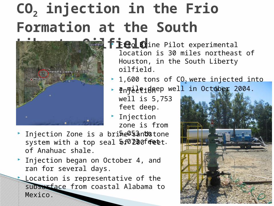
CO2 injection in the Frio Formation at the South Liberty Oilfield Frio Brine Pilot experimental location is 30

miles northeast of Houston, in the South Liberty oilfield. 

1,600 tons of CO2 were injected into a mile-deep well in October 2004.

Injection well is 5,753 feet deep.

Injection zone is from 5,053 to 5,073 feet .  Injection Zone is a brine-sandstone system

with a top seal of 200 feet of Anahuac shale.

Injection began on October 4, and ran for several days.

Location is representative of the subsurface from coastal Alabama to Mexico.

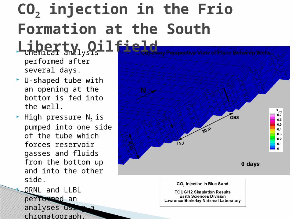
Chemical analysis performed after several days.

U-shaped tube with an opening at the bottom is fed into the well.

High pressure N2 is pumped into one side of the tube which forces reservoir gasses and fluids from the bottom up and into the other side. 

ORNL and LLBL performed an analyses using a chromatograph.

CO2 injection in the Frio Formation at the South Liberty Oilfield

CO2 injection in the Frio Formation at the South Liberty Oilfield Significant findings: injected CO2 causes the brine at depth

to become acidic. Acidic brine dissolves some of the rock and minerals it

comes into contact with, adding iron and other metals to the salt water.

Acidic brine can also allow the brine/CO2 mixture to open new pathways through the sandstone rock and shale cap (via calcite dissolution).

Y.K. Kharaka, D.R. Cole, S.D. Hovorka, W.D. Gunter, K.G. Knauss and B.M. Freifeld, Gas-water-rock interactions in Frio Formation following CO2 injection: Implications for the storage of greenhouse gases in sedimentary basins, Geology; July 2006; v. 34; no. 7; p. 577-580.

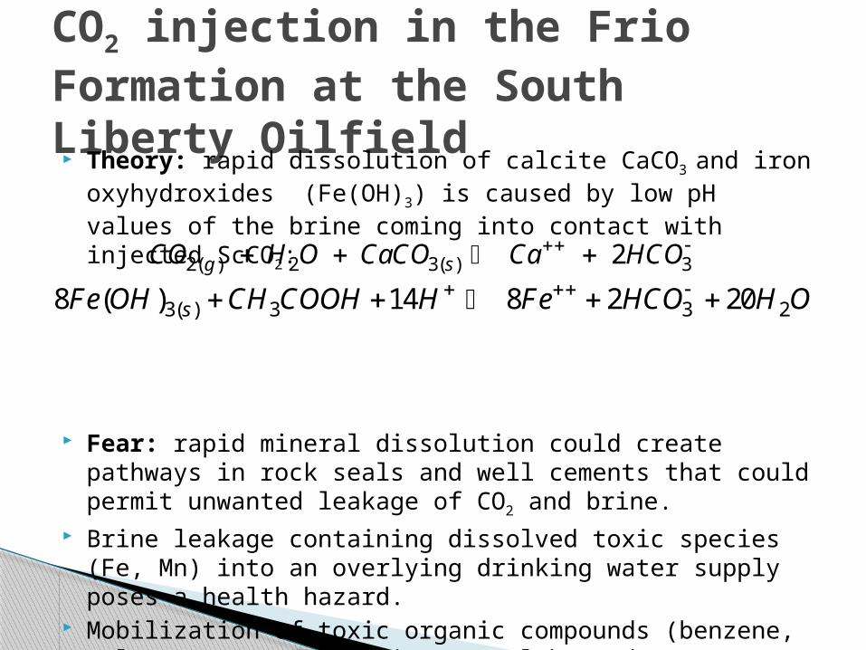
CO2 injection in the Frio Formation at the South Liberty Oilfield Theory: rapid dissolution of calcite CaCO3 and iron

oxyhydroxides  (Fe(OH)3) is caused by low pH values of the brine coming into contact with injected ScCO2:

Fear: rapid mineral dissolution could create pathways in rock seals and well cements that could permit unwanted leakage of CO2 and brine.

Brine leakage containing dissolved toxic species (Fe, Mn) into an overlying drinking water supply poses a health hazard.

Mobilization of toxic organic compounds (benzene, toluene) poses an environmental hazard.

2( ) 2 3( ) 3 2g sCO H O CaCO Ca HCO

3( ) 3 3 28 ( ) 14 8 2 20sFe OH CH COOH H Fe HCO H O

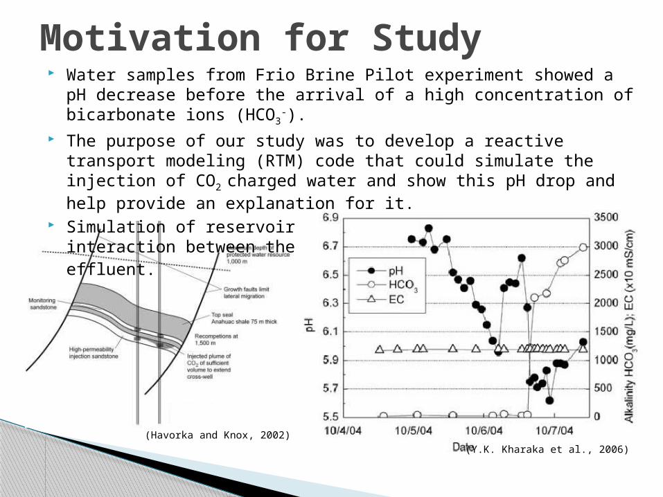
Motivation for Study Water samples from Frio Brine Pilot experiment showed a pH

decrease before the arrival of a high concentration of bicarbonate ions (HCO3

-). The purpose of our study was to develop a reactive transport

modeling (RTM) code that could simulate the injection of CO2

charged water and show this pH drop and help provide an explanation for it.

Simulation of reservoir far from injection well; model interaction between the formation water and CO2(aq) charged effluent.

(Y.K. Kharaka et al., 2006)(Havorka and Knox, 2002)

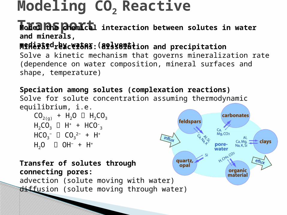
Modeling CO2 Reactive Transport Model the chemical interaction between solutes in water and minerals,mediated by water (solvent)Mineral reactions: dissolution and precipitationSolve a kinetic mechanism that governs mineralization rate (dependence on water composition, mineral surfaces and shape, temperature)

Speciation among solutes (complexation reactions)Solve for solute concentration assuming thermodynamic equilibrium, i.e.

CO2(g) + H2O  H2CO3

H2CO3 H+ + HCO-3

HCO3−  CO3

2− + H+

H2O   OH− + H+

Transfer of solutes through connecting pores:advection (solute moving with water)diffusion (solute moving through water)

2

1 1

Na MeD c c u v A G

t

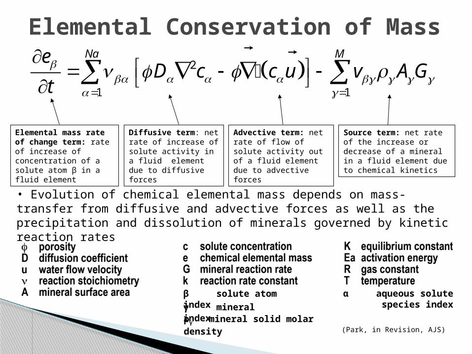
Elemental Conservation of Mass

• Evolution of chemical elemental mass depends on mass-transfer from diffusive and advective forces as well as the precipitation and dissolution of minerals governed by kinetic reaction rates

Elemental mass rate of change term: rate of increase of concentration of a solute atom β in a fluid element

Advective term: net rate of flow of solute activity out of a fluid element due to advective forces

Diffusive term: net rate of increase of solute activity in a fluid element due to diffusive forces

Source term: net rate of the increase or decrease of a mineral in a fluid element due to chemical kinetics

(Park, in Revision, AJS)

β solute atom index α aqueous solute species indexγ mineral index

ργ mineral solid molar density

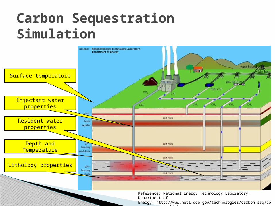
Carbon Sequestration Simulation

Reference: National Energy Technology Laboratory, Department of Energy, http://www.netl.doe.gov/technologies/carbon_seq/core_rd/storage.html 

Depth and Temperature

Surface temperature

Resident water properties

Injectant water properties

Lithology properties

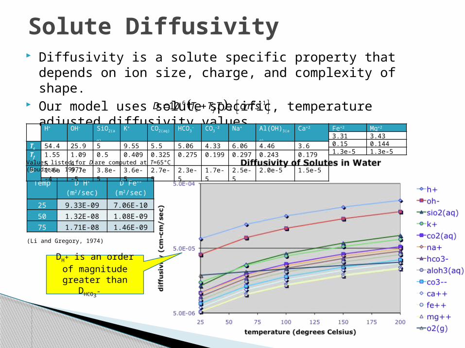
Diffusivity is a solute specific property that depends on ion size, charge, and complexity of shape.

Our model uses solute specific, temperature adjusted diffusivity values.

Solute Diffusivity

Temp D H+ (m2/sec)

D Fe++ (m2/sec)

25 9.33E-09 7.06E-10

50 1.32E-08 1.08E-09

75 1.71E-08 1.46E-09

6 2 110 , c fD T T T cm s

(Li and Gregory, 1974)

H+ OH- SiO2(aq) K+ CO2(aq) HCO3- CO3

-2 Na+ Al(OH)3(aq) Ca+2

Tc 54.4 25.9 5 9.55 5.5 5.06 4.33 6.06 4.46 3.6Tf 1.555 1.094 0.5 0.409 0.325 0.275 0.199 0.297 0.243 0.179D 1.6e-4 9.7e-5 3.8e-5 3.6e-5 2.7e-5 2.3e-5 1.7e-5 2.5e-5 2.0e-5 1.5e-5

Fe+2 Mg+2

3.31 3.430.15 0.1441.3e-5 1.3e-5

Values listed for D are computed at T=65°C (Boudreau, 1997)

DH+ is an order of magnitude greater

than DHCO3-

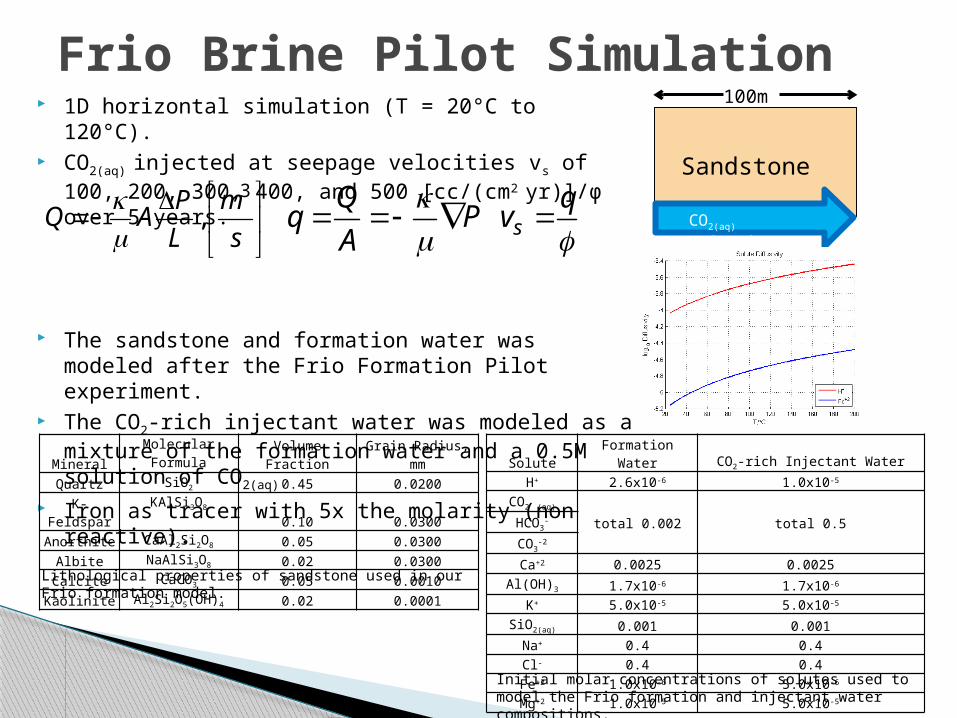
Frio Brine Pilot Simulation

CO2(aq) Injection

100m

Sandstone

1D horizontal simulation (T = 20°C to 120°C). CO2(aq) injected at seepage velocities vs of 100, 200,

300, 400, and 500 [cc/(cm2 yr)]/φ over 5 years.

The sandstone and formation water was modeled after the Frio Formation Pilot experiment.

The CO2-rich injectant water was modeled as a mixture of the formation water and a 0.5M solution of CO2(aq)

Iron as tracer with 5x the molarity (non reactive).

3

,P m

Q AL s

Qq P

A

sq

v

Mineral Molecular Formula Volume Fraction Grain Radius, mmQuartz SiO2 0.45 0.0200

K-Feldspar KAlSi3O8 0.10 0.0300Anorthite CaAl2Si2O8 0.05 0.0300

Albite NaAlSi3O8 0.02 0.0300Calcite CaCO3 0.05 0.0010

Kaolinite Al2Si2O5(OH)4 0.02 0.0001

Solute Formation Water CO2-rich Injectant WaterH+ 2.6x10-6 1.0x10-5

CO2 (aq)

total 0.002 total 0.5HCO3-

CO3-2

Ca+2 0.0025 0.0025Al(OH)3 1.7x10-6 1.7x10-6

K+ 5.0x10-5 5.0x10-5

SiO2(aq) 0.001 0.001Na+ 0.4 0.4Cl- 0.4 0.4Fe+2 1.0x10-6 5.0x10-6

Mg+2 1.0x10-5 5.0x10-5

Lithological properties of sandstone used in our Frio formation model.

Initial molar concentrations of solutes used to model the Frio formation and injectant water compositions.

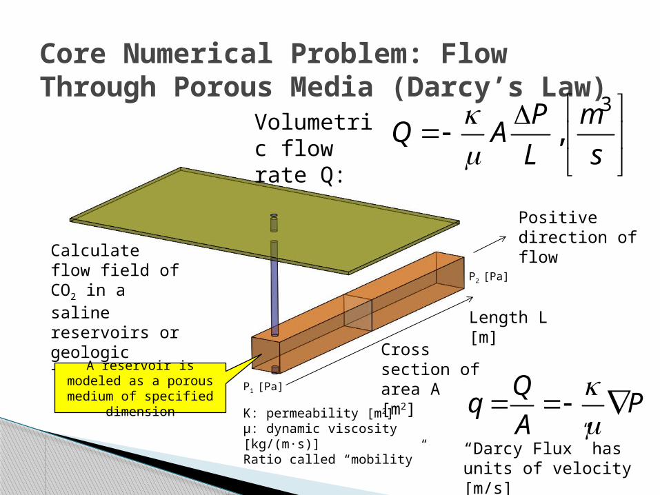
Core Numerical Problem: Flow Through Porous Media (Darcy’s Law)

Calculate flow field of CO2 in a saline reservoirs or geologic formation.

A reservoir is modeled as a porous medium of

specified dimension

Length L [m]

Cross section of area A [m2]

Positive direction of flow

3

,P m

Q AL s

Volumetric flow rate Q:

Κ: permeability [m2]μ: dynamic viscosity [kg/(m∙s)]Ratio called “mobility”

Qq P

A

“Darcy Flux” has units of velocity [m/s]

P2 [Pa]

P1 [Pa]

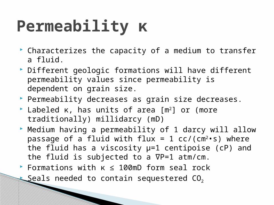
Characterizes the capacity of a medium to transfer a fluid. Different geologic formations will have different

permeability values since permeability is dependent on grain size.

Permeability decreases as grain size decreases. Labeled κ, has units of area [m2] or (more traditionally)

millidarcy (mD) Medium having a permeability of 1 darcy will allow passage

of a fluid with flux = 1 cc/(cm2•s) where the fluid has a viscosity μ=1 centipoise (cP) and the fluid is subjected to a ∇P=1 atm/cm.

Formations with κ ≤ 100mD form seal rock Seals needed to contain sequestered CO2

Permeability κ

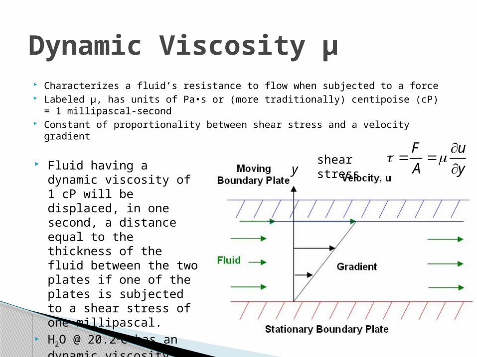
Characterizes a fluid’s resistance to flow when subjected to a force Labeled μ, has units of Pa•s or (more traditionally) centipoise (cP) = 1

millipascal-second Constant of proportionality between shear stress and a velocity gradient

Dynamic Viscosity μ

Fluid having a dynamic viscosity of 1 cP will be displaced, in one second, a distance equal to the thickness of the fluid between the two plates if one of the plates is subjected to a shear stress of one millipascal.

H2O @ 20.2oC has an dynamic viscosity of 1 cP.

F u

A y

shear stressy

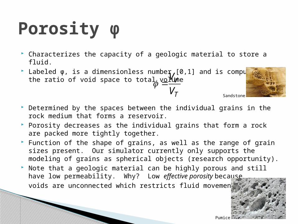
Characterizes the capacity of a geologic material to store a fluid. Labeled φ, is a dimensionless number [0,1] and is computed by the

ratio of void space to total volume

Determined by the spaces between the individual grains in the rock medium that forms a reservoir.

Porosity decreases as the individual grains that form a rock are packed more tightly together.

Function of the shape of grains, as well as the range of grain sizes present. Our simulator currently only supports the modeling of grains as spherical objects (research opportunity).

Note that a geologic material can be highly porous and still have low permeability. Why? Low effective porosity becausevoids are unconnected which restricts fluid movement.

Porosity φ

V

T

V

V

Pumice

Sandstone

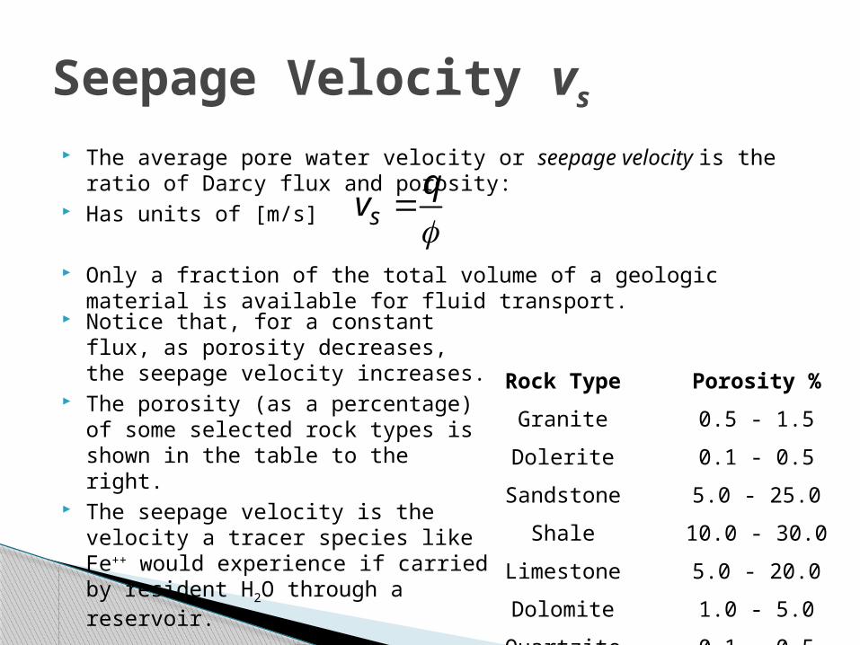
The average pore water velocity or seepage velocity is the ratio of Darcy flux and porosity:

Has units of [m/s]

Only a fraction of the total volume of a geologic material is available for fluid transport.

Seepage Velocity vs

sq

v

Rock Type Porosity %

Granite 0.5 - 1.5

Dolerite 0.1 - 0.5

Sandstone 5.0 - 25.0

Shale 10.0 - 30.0

Limestone 5.0 - 20.0

Dolomite 1.0 - 5.0

Quartzite 0.1 - 0.5

Notice that, for a constant flux, as porosity decreases, the seepage velocity increases.

The porosity (as a percentage) of some selected rock types is shown in the table to the right.

The seepage velocity is the velocity a tracer species like Fe++ would experience if carried by resident H2O through a reservoir.

TOUGHREACT Version 1.2 (YMP Q V3.1.1 July 2006)

TOUGHREACT is a program for non-isothermal reactive fluid flow and geochemical transport in geologic media. It is developed by introducing reactive geochemistry

into the framework of the existing multi-phase fluid and heat flow code TOUGH2 V2.

Developed by Tianfu Xu, Eric Sonnenthal, Nicolas Spycher,and Karsten Pruess at Lawrence Berkeley National Laboratory

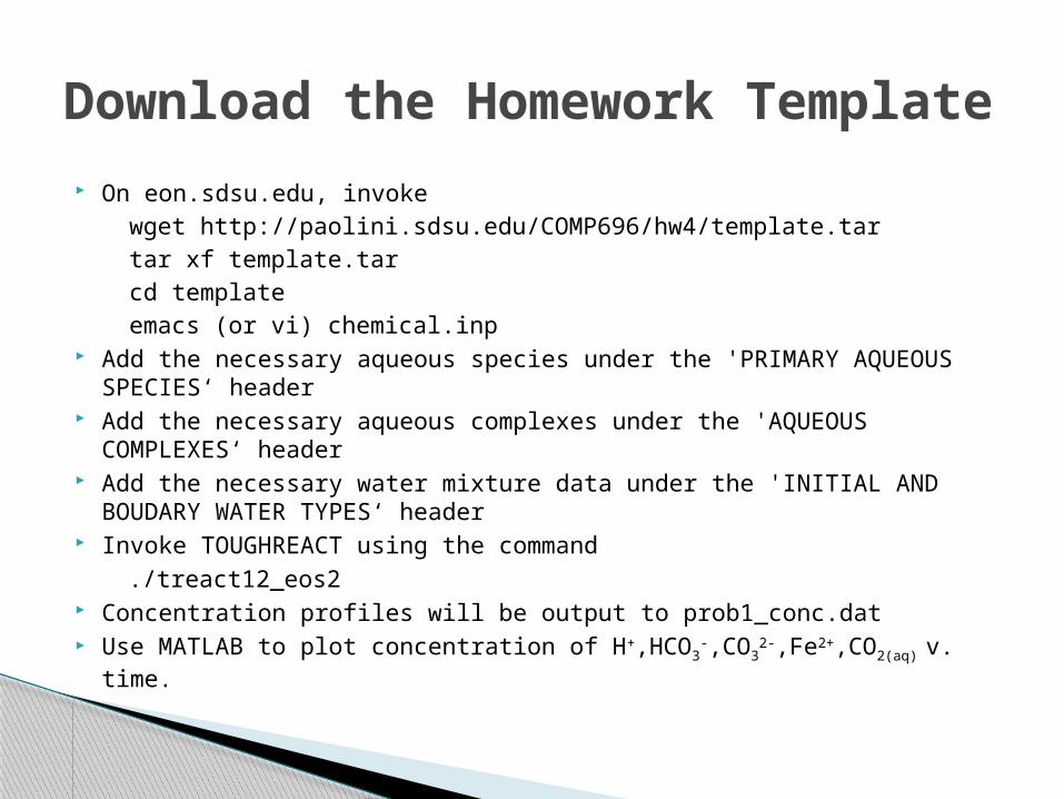
On eon.sdsu.edu, invoke wget http://paolini.sdsu.edu/COMP696/hw4/template.tartar xf template.tarcd templateemacs (or vi) chemical.inp

Add the necessary aqueous species under the 'PRIMARY AQUEOUS SPECIES‘ header

Add the necessary aqueous complexes under the 'AQUEOUS COMPLEXES‘ header

Add the necessary water mixture data under the 'INITIAL AND BOUDARY WATER TYPES‘ header

Invoke TOUGHREACT using the command./treact12_eos2

Concentration profiles will be output to prob1_conc.dat Use MATLAB to plot concentration of H+,HCO3

-,CO32-,Fe2+,CO2(aq) v. time.

Download the Homework Template

Primary Aqueous Species Section'DEFINITION OF THE GEOCHEMICAL SYSTEM''PRIMARY AQUEOUS SPECIES''h2o' 'h+' 'ca+2' 'mg+2' 'na+' 'k+' 'fe+2' 'sio2(aq)' 'hco3-' 'so4-2' 'alo2-' 'cl-' 'o2(aq)' '*'

Start of input chemical.inp file

Start of Primary Aqueous species section

• This section provides a list of aqueous species to use in the simulation. Each species must be on a new line and in single quotes.

• The aqueous species needs to also be in the database file (specified in Solute.inp). Each mineral has a set of aqueous species (also listed in the database file ‘databas1.dat’) that must be included in this list.

• Additional species can also be included, but the minerals aqueous species are required.

Marks end of primary aqueous species section

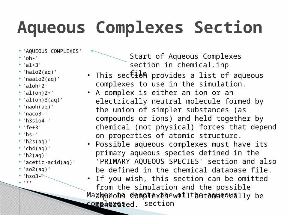
Aqueous Complexes Section

'AQUEOUS COMPLEXES' 'oh-' 'al+3' 'halo2(aq)' 'naalo2(aq)' 'aloh+2' 'al(oh)2+' 'al(oh)3(aq)' 'naoh(aq)' 'naco3-' 'h3sio4-' 'fe+3' 'hs-' 'h2s(aq)' 'ch4(aq)' 'h2(aq)' 'acetic~acid(aq)' 'so2(aq)' 'hso3-' '*'

Start of Aqueous Complexes section in chemical.inp file

• This section provides a list of aqueous complexes to use in the simulation.

• A complex is either an ion or an electrically neutral molecule formed by the union of simpler substances (as compounds or ions) and held together by chemical (not physical) forces that depend on properties of atomic structure. 

• Possible aqueous complexes must have its primary aqueous species defined in the 'PRIMARY AQUEOUS SPECIES' section and also be defined in the chemical database file.

• If you wish, this section can be omitted from the simulation and the possible aqueous complexes will automatically be generated.

Marker to denote the of the aqueous complexes section

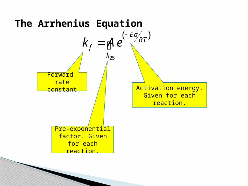
The Arrhenius Equation

25

EaRT

fk

k Ae

Forward rate constant

Pre-exponential factor. Given for each reaction.

Activation energy. Given for each

reaction.

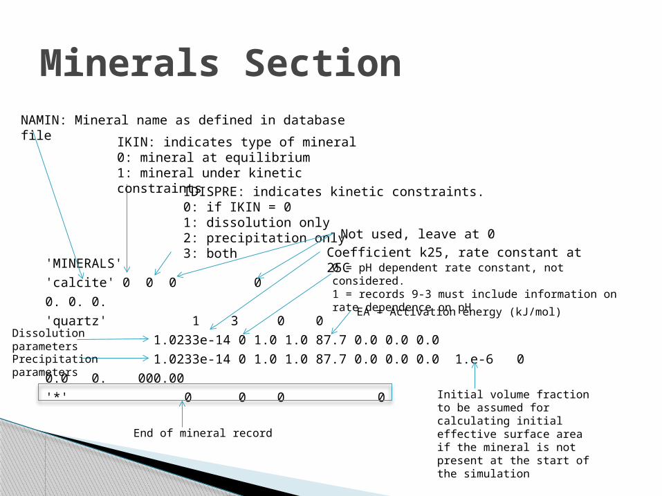
'MINERALS'

'calcite' 0 0 0 0

0. 0. 0.

'quartz' 1 3 0 0

1.0233e-14 0 1.0 1.0 87.7 0.0 0.0 0.0

1.0233e-14 0 1.0 1.0 87.7 0.0 0.0 0.0 1.e-6 0

0.0 0. 000.00

'*' 0 0 0 0

NAMIN: Mineral name as defined in database file

IKIN: indicates type of mineral0: mineral at equilibrium1: mineral under kinetic constraints

IDISPRE: indicates kinetic constraints.0: if IKIN = 01: dissolution only2: precipitation only3: both

Not used, leave at 0Coefficient k25, rate constant at 25C0 = pH dependent rate constant, not considered.1 = records 9-3 must include information on rate dependence on pH

EA = Activation energy (kJ/mol)

Dissolution parametersPrecipitation parameters

Initial volume fraction to be assumed for calculating initial effective surface area if the mineral is not present at the start of the simulation

End of mineral record

Minerals Section

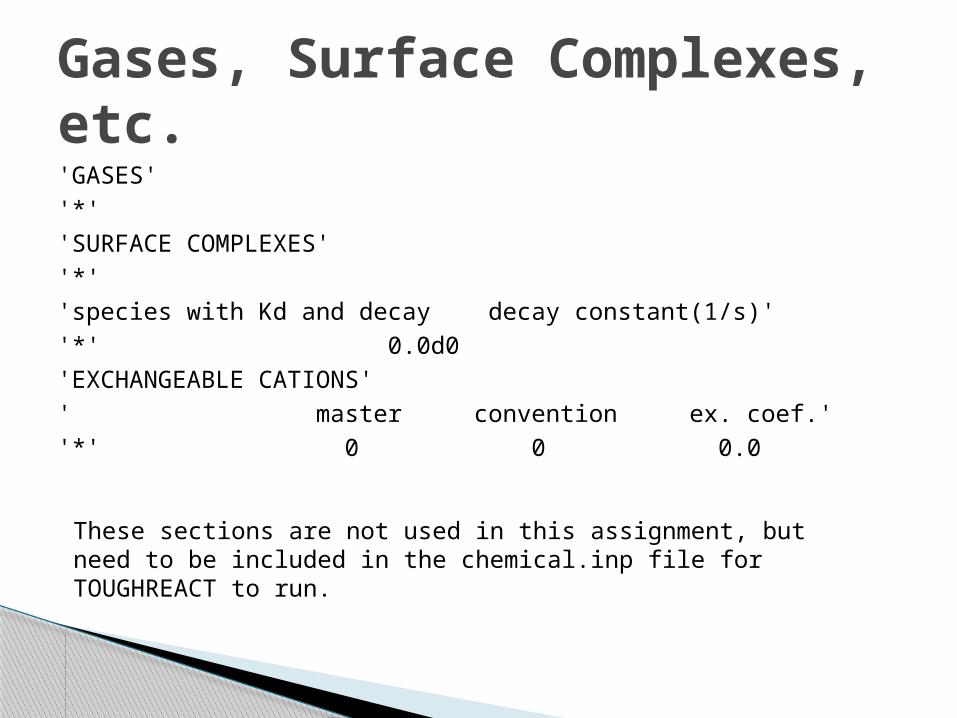
Gases, Surface Complexes, etc.'GASES'

'*'

'SURFACE COMPLEXES'

'*'

'species with Kd and decay decay constant(1/s)'

'*' 0.0d0

'EXCHANGEABLE CATIONS'

' master convention ex. coef.'

'*' 0 0 0.0

These sections are not used in this assignment, but need to be included in the chemical.inp file for TOUGHREACT to run.

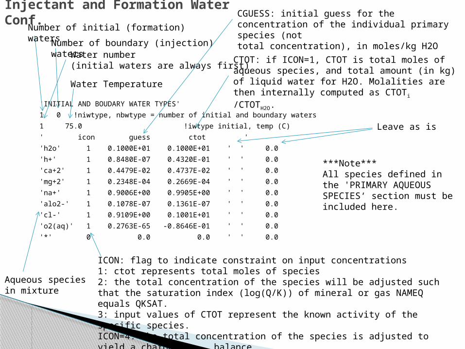
'INITIAL AND BOUDARY WATER TYPES'

1 0 !niwtype, nbwtype = number of initial and boundary waters

1 75.0 !iwtype initial, temp (C)

' icon guess ctot '

'h2o' 1 0.1000E+01 0.1000E+01 ' ' 0.0

'h+' 1 0.8480E-07 0.4320E-01 ' ' 0.0

'ca+2' 1 0.4479E-02 0.4737E-02 ' ' 0.0

'mg+2' 1 0.2348E-04 0.2669E-04 ' ' 0.0

'na+' 1 0.9006E+00 0.9905E+00 ' ' 0.0

'alo2-' 1 0.1078E-07 0.1361E-07 ' ' 0.0

'cl-' 1 0.9109E+00 0.1001E+01 ' ' 0.0

'o2(aq)' 1 0.2763E-65 -0.8646E-01 ' ' 0.0

'*' 0 0.0 0.0 ' ' 0.0

Number of initial (formation) waters

Number of boundary (injection) watersWater number(initial waters are always first)

Water Temperature

Aqueous species in mixture

ICON: flag to indicate constraint on input concentrations1: ctot represents total moles of species2: the total concentration of the species will be adjusted such that the saturation index (log(Q/K)) of mineral or gas NAMEQ equals QKSAT.3: input values of CTOT represent the known activity of the specific species.ICON=4: the total concentration of the species is adjusted to yield a charge

balance.

CGUESS: initial guess for the concentration of the individual primary species (nottotal concentration), in moles/kg H2O

CTOT: if ICON=1, CTOT is total moles of aqueous species, and total amount (in kg) of liquid water for H2O. Molalities are then internally computed as CTOTi /CTOTH2O.

Leave as is

***Note***All species defined in the 'PRIMARY AQUEOUS SPECIES‘ section must be included here.

Injectant and Formation Water Conf.

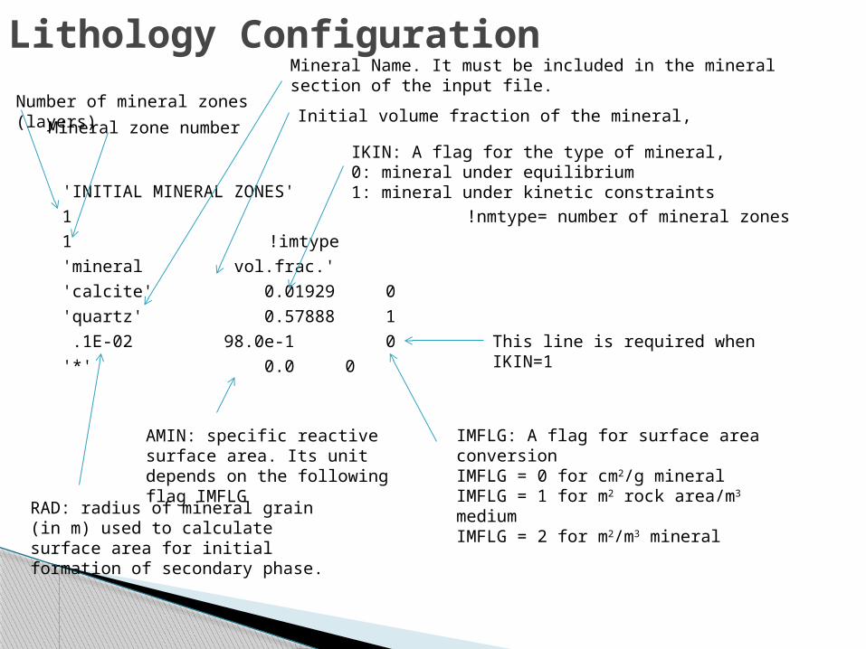
'INITIAL MINERAL ZONES'

1 !nmtype= number of mineral zones

1 !imtype

'mineral vol.frac.'

'calcite' 0.01929 0

'quartz' 0.57888 1

.1E-02 98.0e-1 0

'*' 0.0 0

Number of mineral zones (layers)

Mineral zone number

Mineral Name. It must be included in the mineral section of the input file.

Initial volume fraction of the mineral,

IKIN: A flag for the type of mineral,0: mineral under equilibrium1: mineral under kinetic constraints

This line is required when IKIN=1

RAD: radius of mineral grain (in m) used to calculate surface area for initial formation of secondary phase.

AMIN: specific reactive surface area. Its unit depends on the following flag IMFLG

IMFLG: A flag for surface area conversionIMFLG = 0 for cm2/g mineralIMFLG = 1 for m2 rock area/m3 mediumIMFLG = 2 for m2/m3 mineral

Lithology Configuration

'----------------------------------------------------------------------------'

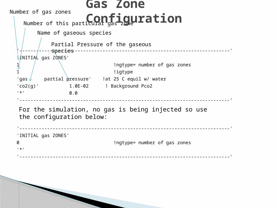
'INITIAL gas ZONES'

1 !ngtype= number of gas zones

1 !igtype

'gas partial pressure' !at 25 C equil w/ water

'co2(g)' 1.0E-02 ! Background Pco2

'*' 0.0

'----------------------------------------------------------------------------‘

'----------------------------------------------------------------------------'

'INITIAL gas ZONES'

0 !ngtype= number of gas zones

'*'

'----------------------------------------------------------------------------‘

Number of gas zones

Number of this particular gas zone

Name of gaseous species

Partial Pressure of the gaseous species

For the simulation, no gas is being injected so use the configuration below:

Gas Zone Configuration

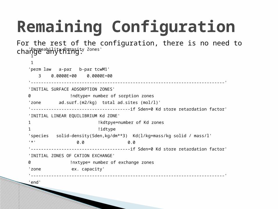
'Permeability-Porosity Zones'

1

1

'perm law a-par b-par tcwM1'

3 0.0000E+00 0.0000E+00

'----------------------------------------------------------------------------'

'INITIAL SURFACE ADSORPTION ZONES'

0 !ndtype= number of sorption zones

'zone ad.surf.(m2/kg) total ad.sites (mol/l)'

'---------------------------------------if Sden=0 Kd store retardation factor'

'INITIAL LINEAR EQUILIBRIUM Kd ZONE'

1 !kdtpye=number of Kd zones

1 !idtype

'species solid-density(Sden,kg/dm**3) Kd(l/kg=mass/kg solid / mass/l'

'*' 0.0 0.0

'---------------------------------------if Sden=0 Kd store retardation factor'

'INITIAL ZONES OF CATION EXCHANGE'

0 !nxtype= number of exchange zones

'zone ex. capacity'

'----------------------------------------------------------------------------'

'end'

For the rest of the configuration, there is no need to change anything:

Remaining Configuration

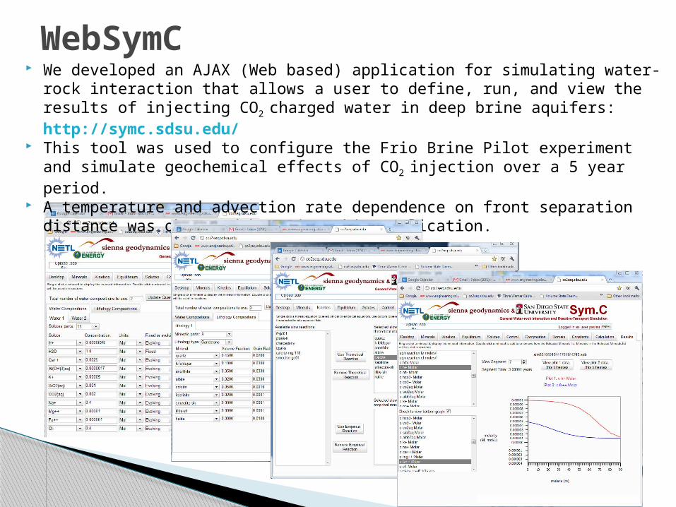
WebSymC We developed an AJAX (Web based) application for simulating water-

rock interaction that allows a user to define, run, and view the results of injecting CO2 charged water in deep brine aquifers: http://symc.sdsu.edu/

This tool was used to configure the Frio Brine Pilot experiment and simulate geochemical effects of CO2 injection over a 5 year period.

A temperature and advection rate dependence on front separation distance was observed by using this application.

Accessing WebSimC Access via URL http://

co2seq.sdsu.edu and http://symc.sdsu.edu/

Supports Google Chrome (recommended), Mozilla Firefox, and Apple Safari.

Does not work with Internet Explorer!

Login with your assigned username and password

WebSim.8 Desktop After logging in, you

will be presented with a drag-and-drop desktop showing the simulations you have configured and invoked to date.

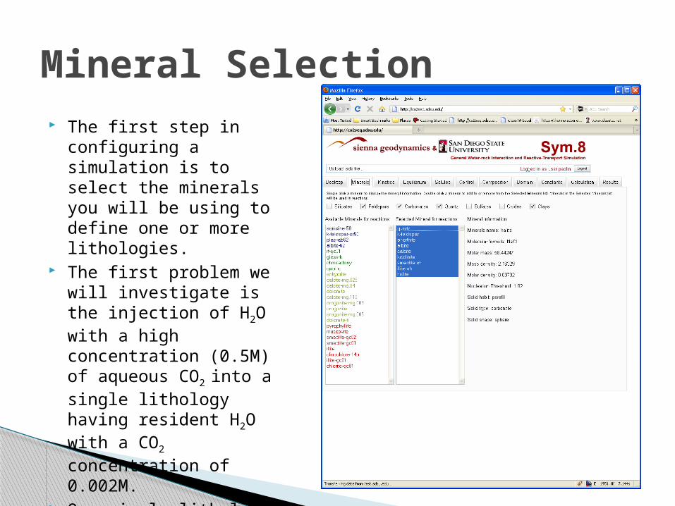
Mineral Selection The first step in

configuring a simulation is to select the minerals you will be using to define one or more lithologies.

The first problem we will investigate is the injection of H2O with a high concentration (0.5M) of aqueous CO2 into a single lithology having resident H2O with a CO2

concentration of 0.002M. Our single lithology will be

sandstone made with the 9 minerals shown.

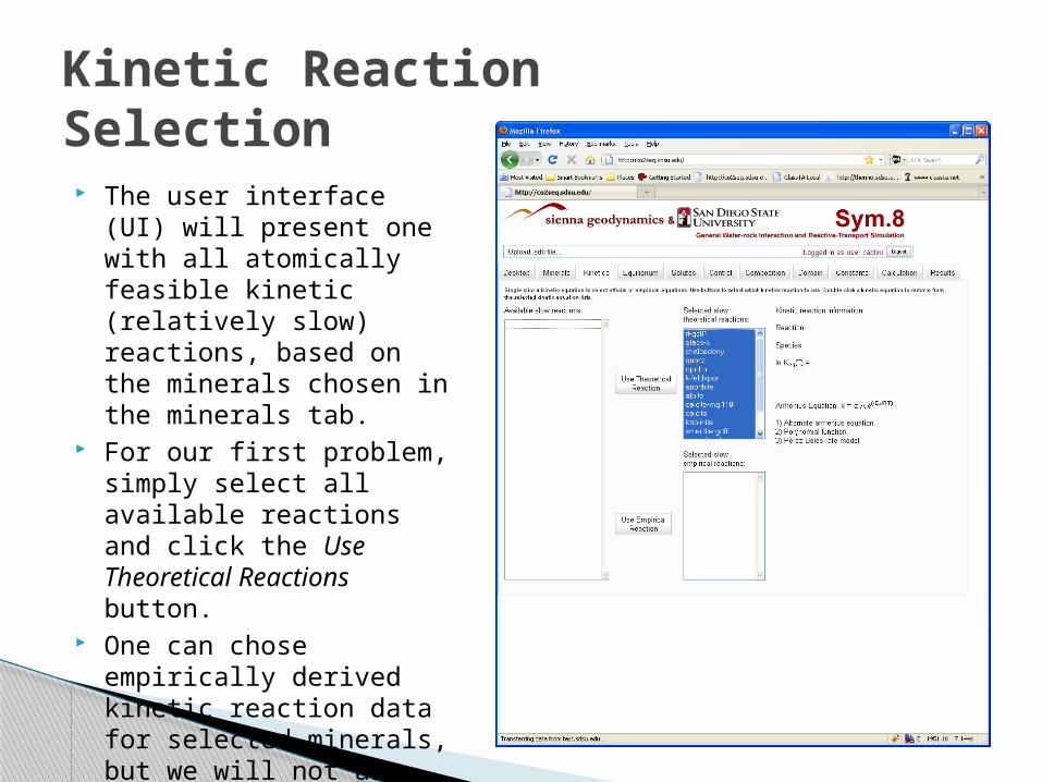
Kinetic ReactionSelection The user interface (UI) will

present one with all atomically feasible kinetic (relatively slow) reactions, based on the minerals chosen in the minerals tab.

For our first problem, simply select all available reactions and click the Use Theoretical Reactions button.

One can chose empirically derived kinetic reaction data for selected minerals, but we will not use this feature for now.

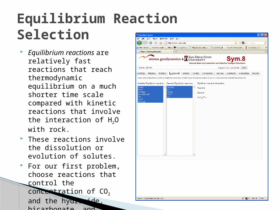
Equilibrium ReactionSelection Equilibrium reactions are

relatively fast reactions that reach thermodynamic equilibrium on a much shorter time scale compared with kinetic reactions that involve the interaction of H2O with rock.

These reactions involve the dissolution or evolution of solutes.

For our first problem, choose reactions that control the concentration of CO2 and the hydroxide, bicarbonate, and

acetate anions.

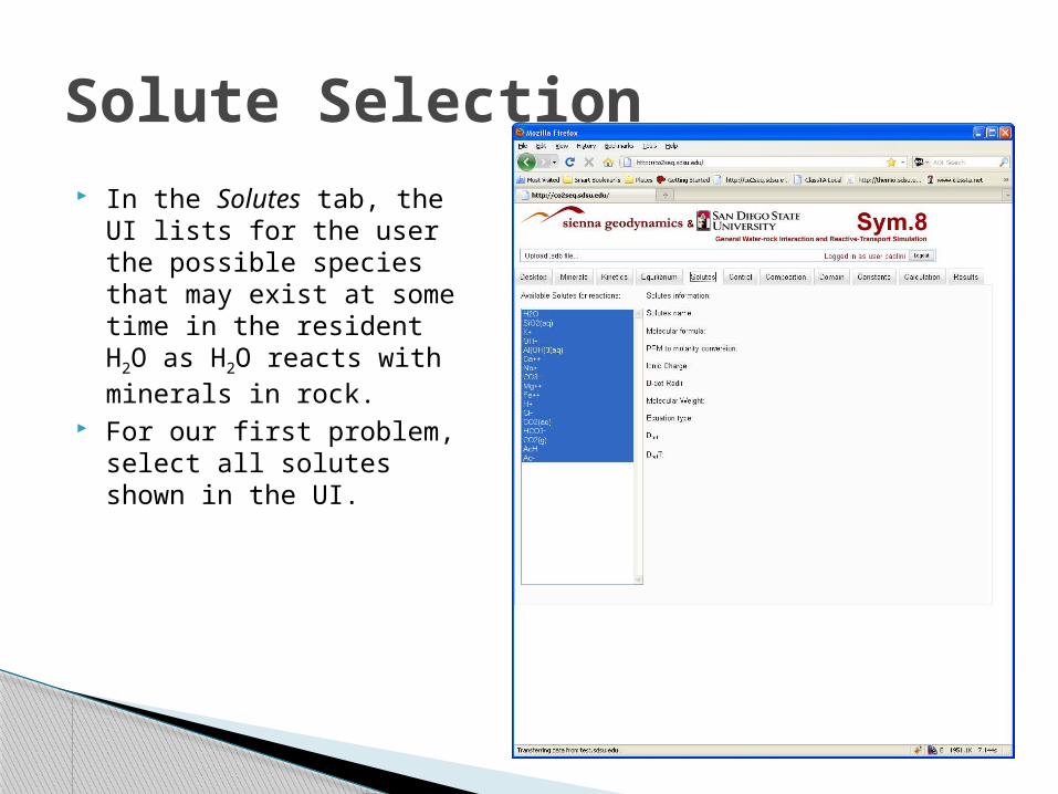
Solute Selection In the Solutes tab, the UI

lists for the user the possible species that may exist at some time in the resident H2O as H2O reacts with minerals in rock.

For our first problem, select all solutes shown in the UI.

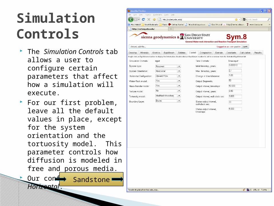
Simulation Controls The Simulation Controls

tab allows a user to configure certain parameters that affect how a simulation will execute.

For our first problem, leave all the default values in place, except for the system orientation and the tortuosity model. This parameter controls how diffusion is modeled in free and porous media.

Our configuration is Horizontal:

Sandstone

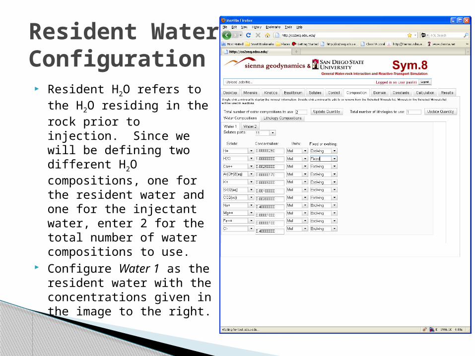
Resident WaterConfiguration Resident H2O refers to the

H2O residing in the rock prior to injection. Since we will be defining two different H2O compositions, one for the resident water and one for the injectant water, enter 2 for the total number of water compositions to use.

Configure Water 1 as the resident water with the concentrations given in the image to the right.

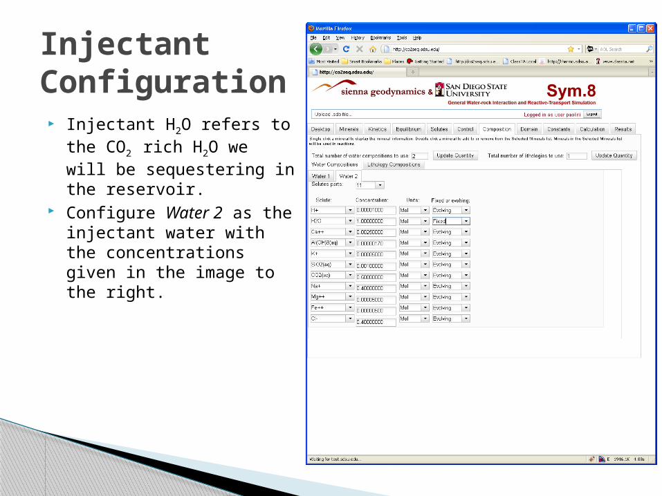
InjectantConfiguration Injectant H2O refers to the

CO2 rich H2O we will be sequestering in the reservoir.

Configure Water 2 as the injectant water with the concentrations given in the image to the right.

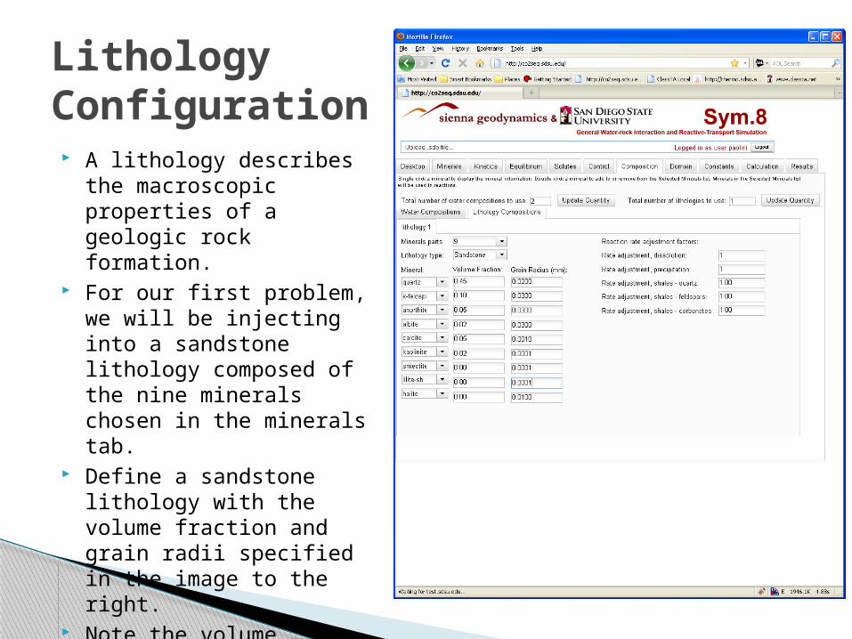
LithologyConfiguration A lithology describes the

macroscopic properties of a geologic rock formation.

For our first problem, we will be injecting into a sandstone lithology composed of the nine minerals chosen in the minerals tab.

Define a sandstone lithology with the volume fraction and grain radii specified in the image to the right.

Note the volume fraction need not sum to 1 as the undefined volume will be Vv.

DomainConfiguration The Lithology sub-tab in the

Domain tab defines the physical characteristics of the reservoir into which we will be injecting CO2 rich H2O.

This tab also defines the numerical grid upon which the resulting system of PDEs will be solved.

For our first problem, select Water 1 as the resident water and define a 100m long section of sandstone with 10 control volumes.

Since we define only one physical dimension, this is a

1D simulation.

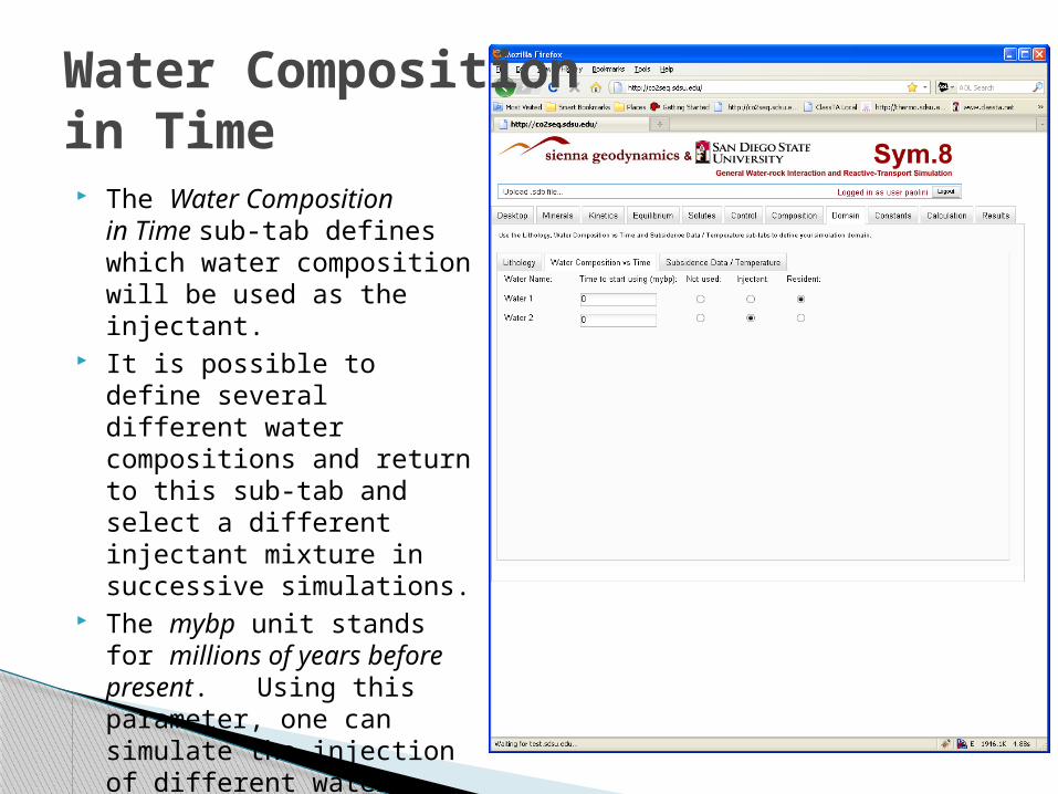
Water Compositionin Time The Water Composition

in Time sub-tab defines which water composition will be used as the injectant.

It is possible to define several different water compositions and return to this sub-tab and select a different injectant mixture in successive simulations.

The mybp unit stands for millions of years before present. Using this parameter, one can simulate the injection of different water compositions at

different times.

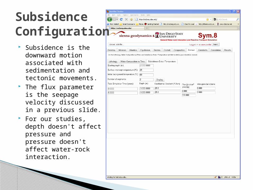
SubsidenceConfiguration Subsidence is the

downward motion associated with sedimentation and tectonic movements.

The flux parameter is the seepage velocity discussed in a previous slide.

For our studies, depth doesn't affect pressure and pressure doesn't affect water-rock interaction.

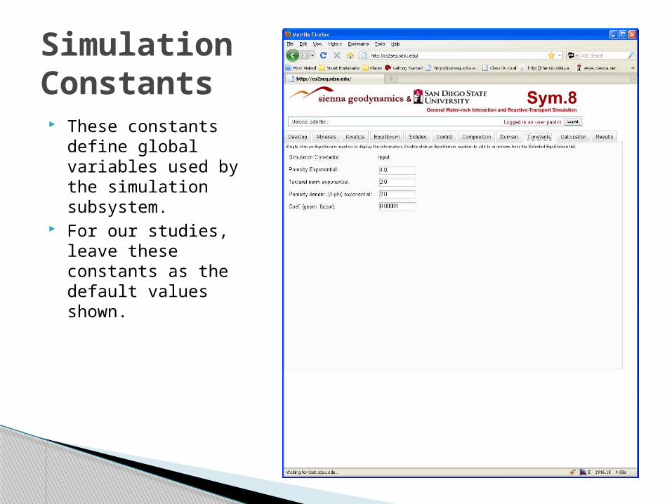
SimulationConstants These constants define

global variables used by the simulation subsystem.

For our studies, leave these constants as the default values shown.

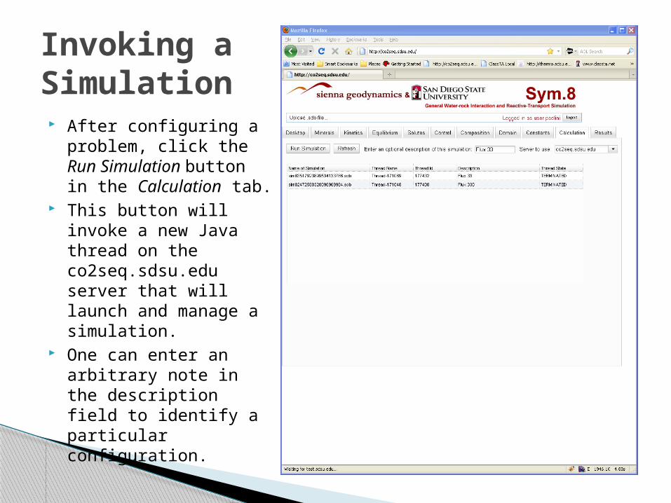
Invoking aSimulation After configuring a

problem, click the Run Simulation button in the Calculation tab.

This button will invoke a new Java thread on the co2seq.sdsu.edu server that will launch and manage a simulation.

One can enter an arbitrary note in the description field to identify a particular configuration.

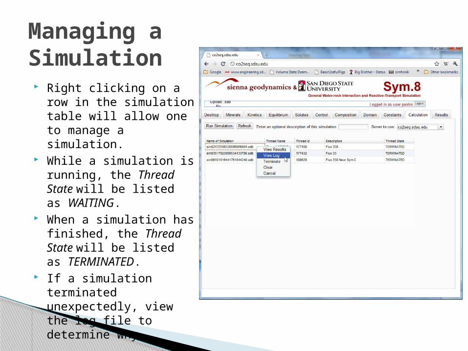
Managing aSimulation Right clicking on a row

in the simulation table will allow one to manage a simulation.

While a simulation is running, the Thread State will be listed as WAITING.

When a simulation has finished, the Thread State will be listed as TERMINATED.

If a simulation terminated unexpectedly, view the log file to determine why.

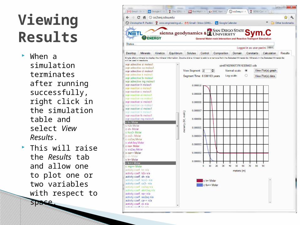
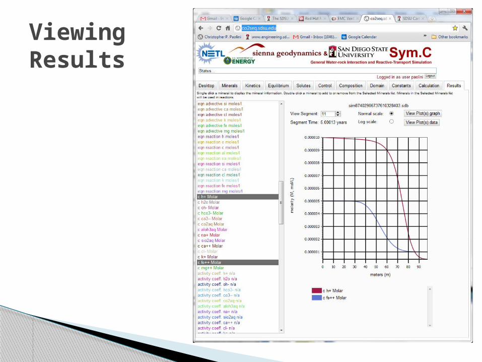
ViewingResults When a

simulation terminates after running successfully, right click in the simulation table and select View Results.

This will raise the Results tab and allow one to plot one or two variables with respect to space.

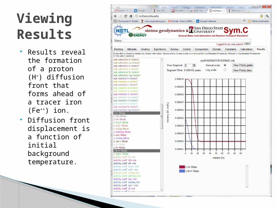
ViewingResults Results reveal the

formation of a proton (H+) diffusion front that forms ahead of a tracer iron (Fe++) ion.

Diffusion front displacement is a function of initial background temperature.

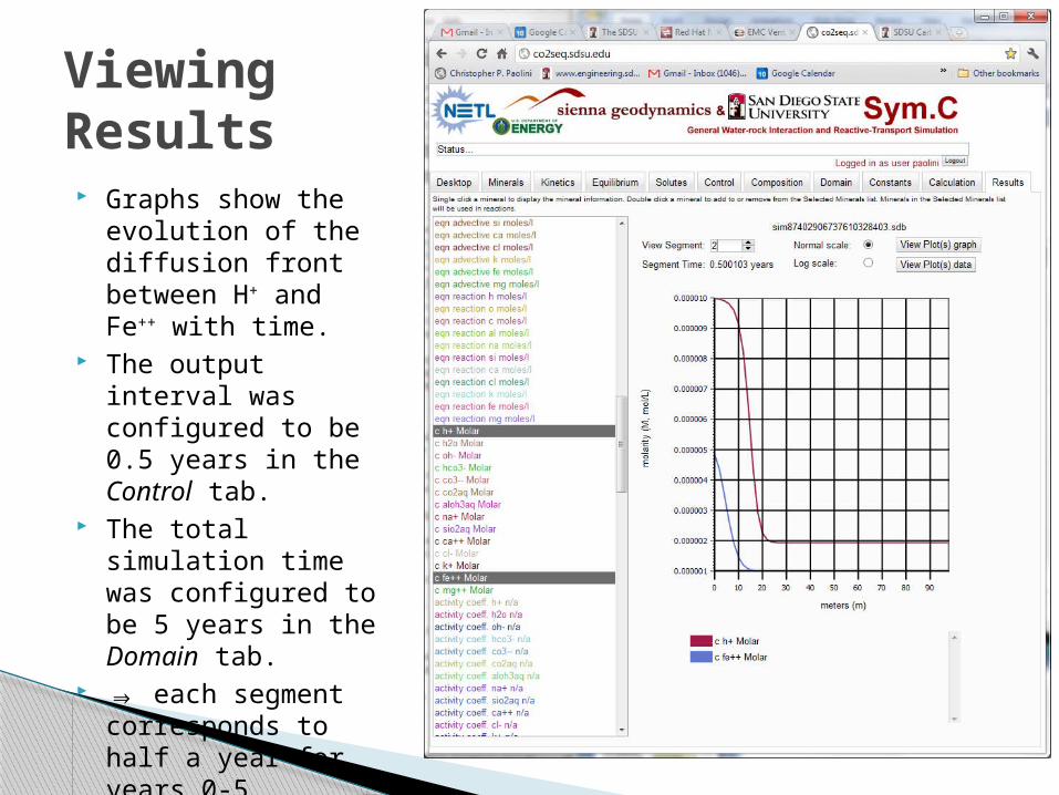
ViewingResults Graphs show the

evolution of the diffusion front between H+ and Fe+

+ with time. The output interval

was configured to be 0.5 years in the Control tab.

The total simulation time was configured to be 5 years in the Domain tab.

⇒ each segment corresponds to half a year for years 0-5.

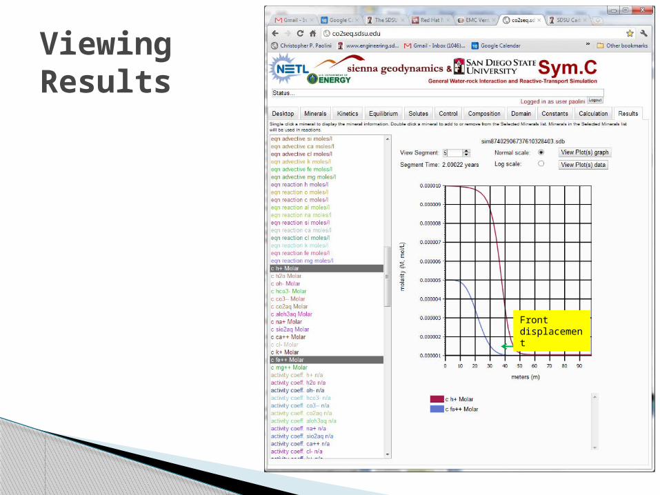
ViewingResults

Front displacement

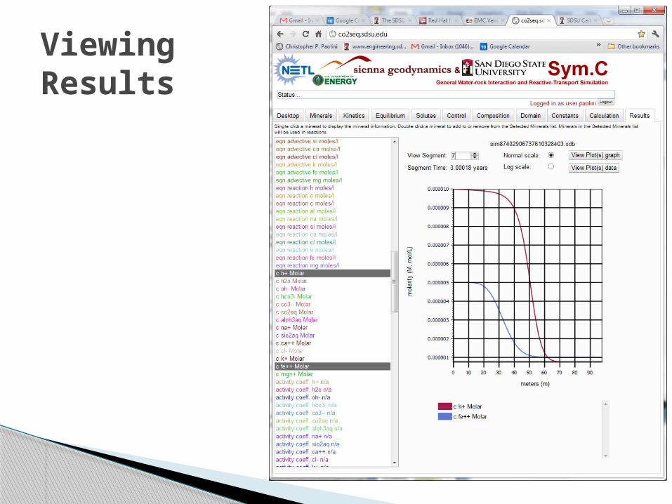
ViewingResults

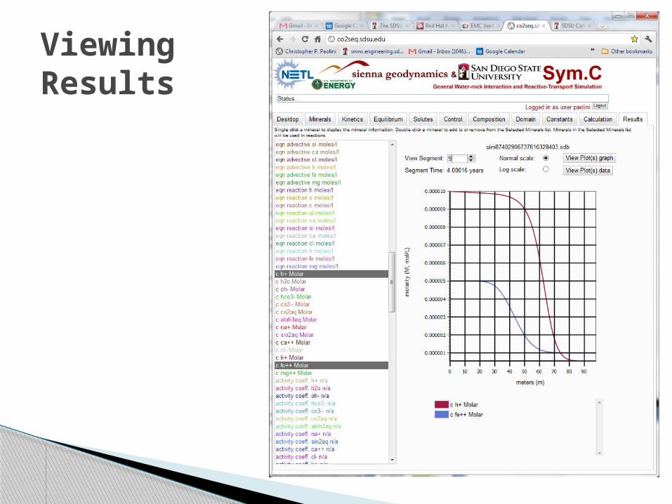
ViewingResults

ViewingResults

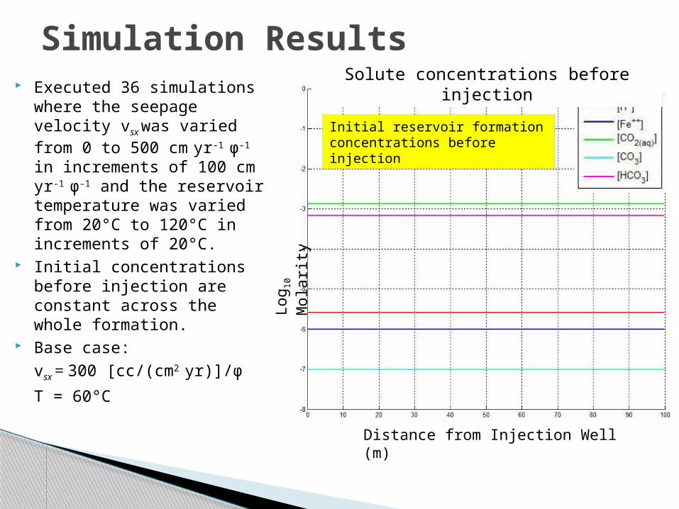
Simulation Results

Initial reservoir formation concentrations before injection

Distance from Injection Well (m)

Log

10 M

ola

rity

Solute concentrations before injection Executed 36 simulations

where the seepage velocity vsx was varied from 0 to 500 cm yr-1 φ-1 in increments of 100 cm yr-1 φ-1 and the reservoir temperature was varied from 20°C to 120°C in increments of 20°C.

Initial concentrations before injection are constant across the whole formation.

Base case: vsx = 300 [cc/(cm2 yr)]/φ

T = 60°C

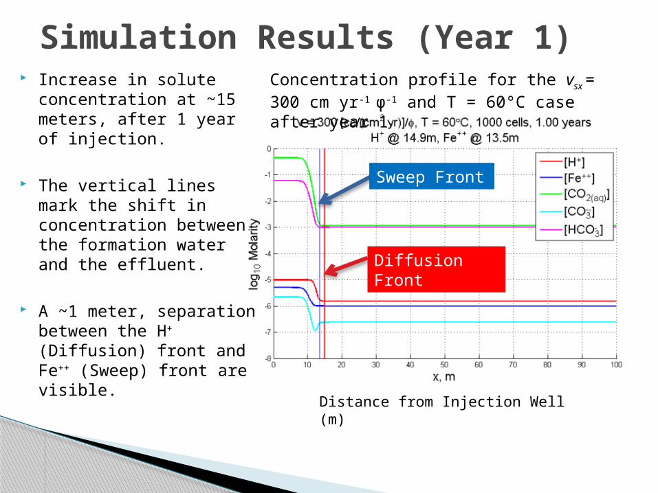
Simulation Results (Year 1) Increase in solute

concentration at ~15 meters, after 1 year of injection.

The vertical lines mark the shift in concentration between the formation water and the effluent.

A ~1 meter, separation between the H+ (Diffusion) front and Fe++ (Sweep) front are visible.

Distance from Injection Well (m)

Diffusion Front

Sweep Front

Concentration profile for the vsx = 300 cm yr-1 φ-1 and T = 60°C case after year 1

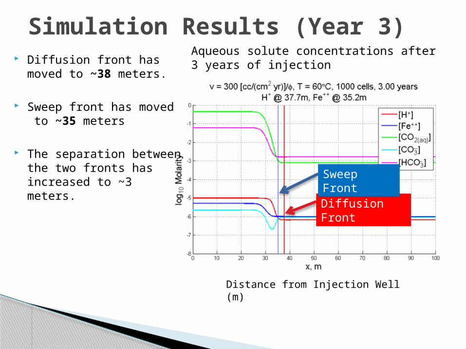
Simulation Results (Year 3) Diffusion front has moved

to ~38 meters.

Sweep front has moved to ~35 meters

The separation between the two fronts has increased to ~3 meters.

Diffusion Front

Sweep Front

Aqueous solute concentrations after 3 years of injection

Distance from Injection Well (m)

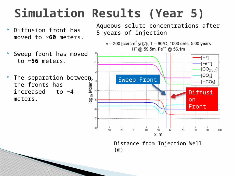
Simulation Results (Year 5)

Diffusion Front

Sweep Front

Diffusion front has moved to ~60 meters.

Sweep front has moved to ~56 meters.

The separation between the fronts has increased to ~4 meters.

Distance from Injection Well (m)

Aqueous solute concentrations after 5 years of injection

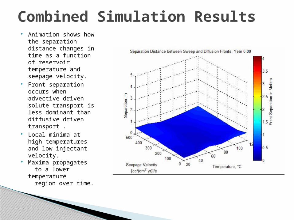
Combined Simulation Results Animation shows

how the separation distance changes in time as a function of reservoir temperature and seepage velocity.

Front separation occurs when advective driven solute transport is less dominant than diffusive driven transport .

Local minima at high temperatures and low injectant velocity.

Maxima propagates to a lower

temperature region over time.

Simulation Results

Distance from injection well (m)

Diffusion Front

Sweep Front

Front Separation

log

10 M

ola

rity

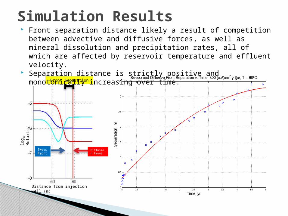
Front separation distance likely a result of competition between advective and diffusive forces, as well as mineral dissolution and precipitation rates, all of which are affected by reservoir temperature and effluent velocity.

Separation distance is strictly positive and monotonically increasing over time.

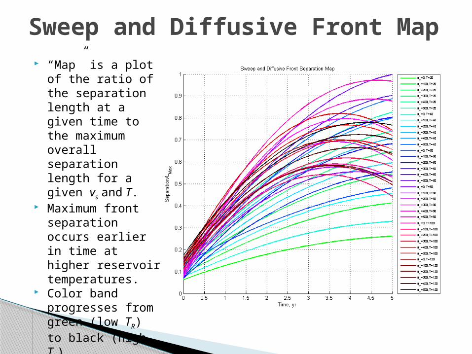
Sweep and Diffusive Front Map “Map” is a plot of

the ratio of the separation length at a given time to the maximum overall separation length for a given vs and T.

Maximum front separation occurs earlier in time at higher reservoir temperatures.

Color band progresses from green (low TR) to black (high TR).

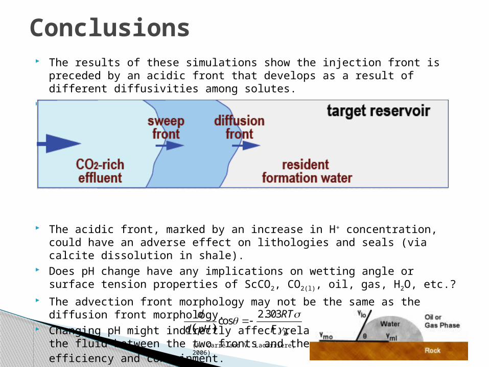
The results of these simulations show the injection front is preceded by an acidic front that develops as a result of different diffusivities among solutes.

Abundant CO2 in the effluent is a constant source of H+ and bicarbonates.

The acidic front, marked by an increase in H+ concentration, could have an adverse effect on lithologies and seals (via calcite dissolution in shale).

Does pH change have any implications on wetting angle or surface tension properties of ScCO2, CO2(l), oil, gas, H2O, etc.?

The advection front morphology may not be the same as the diffusion front morphology.

Changing pH might indirectly affect relative permeability of the fluid between the two fronts and thereby affect CO2 storage efficiency and containment.

Conclusions

lo

2.303cos

d RT

d pH F

(A. Carré and V. Lacarrière, 2006)

When CO2 rich water is injected into a deep brine formation, carbonic acid is produced, which dissociates to form bicarbonate.

The bicarbonate ion also dissociates, albeit to a lesser extent, to form carbonate.

Possible Implications in CO2

Storage

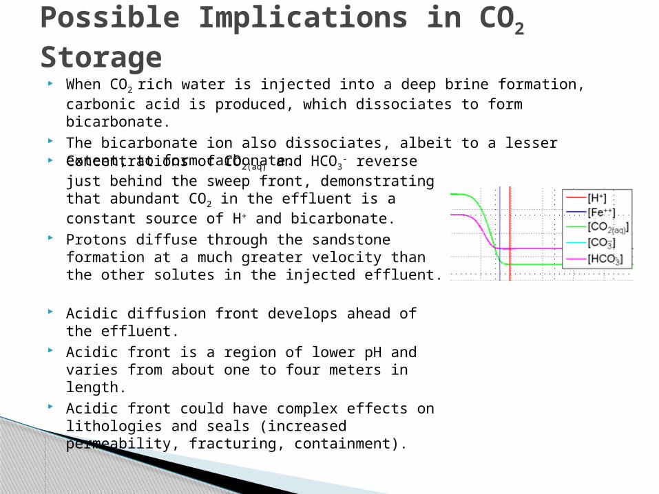
Concentrations of CO2(aq) and HCO3- reverse just

behind the sweep front, demonstrating that abundant CO2 in the effluent is a constant source of H+ and bicarbonate.

Protons diffuse through the sandstone formation at a much greater velocity than the other solutes in the injected effluent.

Acidic diffusion front develops ahead of the effluent. Acidic front is a region of lower pH and varies from

about one to four meters in length. Acidic front could have complex effects on

lithologies and seals (increased permeability, fracturing, containment).

Acidic Front Effect on Mineral Saturation

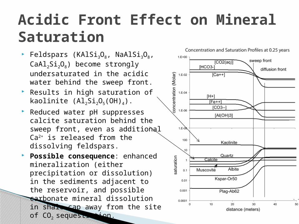
Feldspars (KAlSi3O8, NaAlSi3O8, CaAl2Si2O8) become strongly undersaturated in the acidic water behind the sweep front.

Results in high saturation of kaolinite (Al2Si2O5(OH)4).

Reduced water pH suppresses calcite saturation behind the sweep front, even as additional Ca2+ is released from the dissolving feldspars.

Possible consequence: enhanced mineralization (either precipitation or dissolution) in the sediments adjacent to the reservoir, and possible carbonate mineral dissolution in shale cap away from the site of CO2 sequestration.