Christina Tavolato and Lars Isaksen Research Department · 744 On the use of a Huber norm for...

744

On the use of a Huber norm forobservation quality control in the

ECMWF 4D-Var

Christina Tavolato1,2 and Lars Isaksen

Research Department

1ECMWF2Department of Meteorology and Geophysics, University of Vienna,

Austria

Submitted to QJRMS

November 2014

Series: ECMWF Technical Memoranda

A full list of ECMWF Publications can be found on our web site under:http://www.ecmwf.int/en/research/publications

Contact: [email protected]

c©Copyright 2014

European Centre for Medium-Range Weather ForecastsShinfield Park, Reading, RG2 9AX, England

Literary and scientific copyrights belong to ECMWF and are reserved in all countries. This publicationis not to be reprinted or translated in whole or in part without the written permission of the Director-General. Appropriate non-commercial use will normally be granted under the condition that referenceis made to ECMWF.

The information within this publication is given in good faith and considered to be true, but ECMWFaccepts no liability for error, omission and for loss or damage arising from its use.

On the use of a Huber norm for observation quality control in the ECMWF 4D-Var

Abstract

This paper describes a number of important aspects that need to be considered when designing andimplementing an observation quality control scheme in an NWP data assimilation system. It is shownhow careful evaluation of innovation statistics provides valuable knowledge about the observationerrors and help in the selection of a suitable observation error model. The focus of the paper ison the statistical specification of the typical fat tails of the innovation distributions. In observationerror specifications, like the one used previously at ECMWF (European Centre for Medium-RangeWeather Forecasts), it is common to assume outliers to represent gross errors that are independentof the atmospheric state. The investigations in this paper show that this is not a good assumptionfor almost all observing systems used in today’s data assimilation systems. It is found that a Hubernorm distribution is a very suitable distribution to describe most innovation statistics, after discardingsystematically erroneous observations. The Huber norm is a robust method, making it safer to includeoutlier observations in the analysis step. Therefore the background quality control can safely berelaxed. The Huber norm has been implemented in the ECMWF assimilation system for in-situobservations. The design, implementation and results from this implementation are described inthis paper. The general impact of using the Huber norm distribution is positive, compared to thepreviously used variational quality control method that gave virtually no weight to outliers. Casestudies show how the method improves the use of observations, especially for intense cyclones andother extreme events. It is also discussed how the Huber norm distribution can be used to identifysystematic problems with observing systems.

1 Introduction

Quality control (QC) of observations [Lorenc and Hammon (1988)] is an important component of anydata assimilation system. Observations have measurement errors and sometimes gross errors due totechnical errors, human errors or transmission problems. The goal is to ensure that correct observationsare used and erroneous observations are discarded from the analysis process. It has long been recognisedthat a good quality control process is required because adding erroneous observations to the assimilationcan lead to spurious features in the analysis [Lorenc (1984)].

In data assimilation the use of departures of observations (o) from the short-range (background, b) fore-cast is an integral part of the QC. If observations, evaluated over a long period, systematically or errati-cally deviate from the background forecast they should be blacklisted, i.e., not taken into account at all inthe analysis [Hollingsworth et al. (1986)]. The remaining observations are, for each analysis cycle, alsocompared against the background and rejected if the background departures are large. Often departures,normalised by the expected observation error, are assumed to follow a Gaussian distribution. This meansoutliers are statistically very unlikely and will unjustly get the same full weight in the analysis as cor-rect observations, increasing the risk of producing an erroneous analysis by using incorrect observations.This is usually resolved by applying fairly tight background departure limits that rejects outliers. Thebackground QC limits depend on the specified observation error and background error. For accurate ob-servations and modern high quality assimilation systems these are both small, e.g., of the order of 0.5hPafor automated surface pressure observations. So surface pressure observations will typically be rejectedif they differ by more than about 4hPa from background fields, corresponding to six standard deviationsof normalised departures. In most cases this is reasonable, but for extreme events it may well happenthat the short-range forecast is wrong by more than 4hPa near the centre of cyclones. The QC decisionscan be improved to some degree by introducing flow-dependent, more accurate, background errors, likethe ones recently implemented at ECMWF [Isaksen et al. (2010), Bonavita et al. (2012)]. These errorswould typically be larger near the centre of cyclones.

Technical Memorandum No. 744 1


Section 2 of the paper investigates the innovation statistics for some of the most important in-situ obser-vations. This leads to a discussion and description in section 3 of the gross error quality control aspectsthat needs to be considered for observations. The special problems that may occur for biases and biascorrection of isolated stations is covered in section 4. After this general study of innovation statistics andgross error characteristics, section 5 describes a range of proposed probability distributions with fat tailsthat are candidates for innovation statistics and observation error specification. Based on the informationpresented in sections 2-5 it is found that a Huber norm [Huber (1964), Huber (1972)] is the most suitabledistribution to use. The method allows the inclusion of outliers in the analysis with reduced weight,because it is a robust estimation method. This is in contrast with a pure Gaussian approach where theanalysis can be ruined by a few erroneous outliers. Section 6 covers the aspects that need to be con-sidered when implementing a Huber norm QC in a NWP system. It is described how this is done inthe Integrated Forecast System (IFS) at ECMWF, where it has been used operationally since September2009. It is also explained how the background quality control has been relaxed, and how observationerror values have been reduced at the centre of the distribution to consistently reflect the Huber normdistribution. Section 7 presents general impact results and a number of case studies.

2 Distribution of departure statistics for some important in-situ observa-tions

The main weakness of using background departure statistics for investigations of observation error distri-butions is that they are a convolution of observation and background information. Further information isrequired to uniquely determine the observation-related distribution, which is what we really are trying toestimate, as it is needed in the definition of the observation cost function. Despite this weakness innova-tion statistics are the most common observation related diagnostics used in data assimilation. Additionalresearch to identify if background errors are non-Gaussian is recommended, but it is outside the scope ofthis paper. Assuming the background errors follow a Gaussian distribution, all non-Gaussian aspects ofthe innovation distribution can be assigned to the observation error distribution. Evaluation of the tails ofinnovation distributions is also likely to provide valuable information about the tails of the observationdistributions.

The QC aspects are primarily related to small number of observations in the tails of the distribution. Soto get a sufficiently large sample of relevant departure statistics 18 months’ worth of data assimilationsystem departure statistics (February 2006 to September 2007) was used for these estimates. This wasdone for a large number of observation types, to determine the distributions that best represented thenormalised departures for each of these sets. The model background fields are from the operationalincremental 4D-Var assimilation system [Courtier et al. (1994)] at ECMWF, taken at appropriate time(± 15 minutes) and at T799L91 (25km horizontal grid and 91 levels outer loop) resolution.

Figure 1 shows the departure distributions, normalised by the prescribed observation error, for a numberof these observation types. The grey crosses represent the data counts for bins of width 0.1 in the range± 10 of normalised departures. Traditionally this would be plotted as histograms, but crosses wereeasier to see on the figures. To put the focus on the tails of the distribution, the data are plotted on asemi-logarithmic scale. This means a Gaussian distribution shows up as a quadratic function, and anexponential distribution as a linear function. On the figure the best fit Gaussian distributions (dashed-dotted line) are included. Figure 1a shows temperature data in the 150-250hPa range for all Vaisala RS92radiosonde measurements in the Northern Hemisphere extra-tropics. A similar plot for the used data isshown in Figure 1b (used data is defined as quality controlled data with more than 25% weight after

2 Technical Memorandum No. 744


applying the previously used ”Gaussian plus flat” distribution QC). The ”Gaussian plus flat” distributionQC and its implementation at ECMWF is described in [Andersson and Jarvinen(1999)] (abbreviatedAJ99). Vaisala RS92 radiosondes are known to be of very high quality with very low bias, very few grosserrors, and with low random errors. Panels c-f in Figure 1 show normalised departure statistics for otherconventional observation types and their data distributions for the extra-tropical regions. Panels c and dshow two different surface pressure observing systems (land surface pressure in the Southern Hemisphereextra-tropics and ship surface pressure in the Northern Hemisphere extra-tropics) and panels e and f showupper air and surface wind observations (aircraft winds from all levels in the Northern Hemisphere extra-tropics and winds observed by drifting buoys in the Northern Hemisphere extra-tropics).

The solid black curves on Figure 1 show the best fit Huber norm distribution. The Huber norm, aGaussian distribution with exponential distribution tails, is defined in section 5 Eq. 1. Because f in Eq.1 is first order continuous the Huber norm distribution shows up as a quadratic function that smoothlytransforms into a linear function in the tails of the distribution. It is seen that the background departurestatistics are well described by a Huber norm distribution, because the data in the tails are in goodagreement with the solid black curves. Indeed, these results indicate that the Huber norm distributionfits the data much better than a pure Gaussian distribution (dash-dotted curves). The Gaussian plus flatdistribution that previously was used in the operational assimilation system at ECMWF is included onFigure 1a as a thick solid grey curve. It is evident that the Gaussian plus flat represents the tails ofthe normalised departure distribution very poorly for radiosonde observations. This is the case for allthe variables shown in Figure 1, and for almost all other observation types that have been investigated(not shown). It is worth mentioning that a sum of Gaussian distributions does not produce a Huberdistribution. So this is not the explanation for the fat tails.

It is noted that there is a factor of more than 1000 between the data counts in the tails (at 8-9 normaliseddepartures). At the centre of the distribution (up to 2 normalised departures), departures are close to aGaussian distribution for most observations. There are no indications of flat tailed distributions, i.e., noindication of standard gross errors where the observed value is unrelated to the background field. Thereis rather an indication of an exponential distribution for many observations in the range 2-9 normaliseddepartures. For the used data (Figure 1b) the departures to large extent follow a Gaussian distribution.This is because the departures are from the pre-2009 operational assimilation system at ECMWF thatapplied the ”Gaussian plus flat” QC distribution, resulting in a sharp transition from full Gaussian weightto zero weight, as shown schematically in Figure 5b.

3 Gross error quality control aspects for observations

Extensive investigation of the normalised background departure statistics for many different observationtypes and parameters gave a useful insight into gross error aspects. Most distributions have fatter thanGaussian distributions beyond 1-2 normalised departures. The reason why there are only few examples offlat distributions in the tails may well be due to most observing systems now are automated. Automatedsystems reduce human related gross errors like swapped latitude/longitude, E/W sign error and swappeddigits. If innovation statistics from a station or platform show flat tail gross error characteristics, it willoften be due to a systematic malfunctioning that results in all observations being wrong. It is fairly easyto detect and eliminate (”blacklist”) these observations via a pre-analysis monitoring procedure. Theywill then not be part of the observations presented to the analysis. We will now give some examples thathighlight these issues.



N: 630794

b

Huber: 2.2 1.6N: 640543

10000

1000

100

10

–10 –5 0 5 10

–10 –5 0 5 10

–10 –5 0 5 10

–10 –5 0 5 10

–10 –5 0 5 10

–10 –5 0 5 10

1

10000

1000

100

10

1

10000

1000

100

10

1

10000

1000

100

10

1

10000

100000

1000

100

10

1

1000

100

10

1

a

Huber: 1.6 1.3

N: 881820

d

Huber: 0.1 0.1N: 1932388

c

Huber: 0.7 0.8

N: 79397

f

Huber: 0.8 0.9N: 12953866

e

Huber: 1.3 1.3

Figure 1: Panels a and b: Innovation statistics, normalised by the prescribed observation error, for all and usedVaisala RS92 radiosonde temperature observations from 150-250hPa in the Northern Hemisphere extra-tropics.c) SYNOP surface pressure observations in the Southern Hemisphere extra-tropics, d) SHIP surface pressureobservations in the Northern Hemisphere extra-tropics, e) aircraft wind observations in the Northern Hemisphereextra-tropics and f) DRIBU wind observations in the Northern Hemisphere extra-tropics. The best fit Gaussiandistribution (dash-dotted) and Huber norm distribution (solid) are included. Panel a) also shows the best fitGaussian plus flat distribution (fat solid grey).



N: 896964

b

Huber: 0.9 0.9N: 1057115

a

Huber: 0.2 0.3

N: 3367349

d

Huber: 1.5 1.4N: 28850428

c

Huber: 1.0 1.0

–10 –5 0 5 10–10 –5 0 5 10

–10 –5 0 5 10–10 –5 0 5 10

10000

1000

100

10

1

10000

100000

1000

100

10

1

10000

100000

1000

100

10

1

10000

100000

1000

100

10

1

Figure 2: Departure statistics for: a) temperature data for all AMDAR (primarily data from European, Chineseand Japanese aircraft) descending over the Northern Hemisphere extra-tropics, b) similar to a), but for ACARS(primarily data from North American aircraft). c) Synop surface pressure, d) Metar surface pressure. In this panelthe black dots show the data before blacklisting.

3.1 Chinese aircraft temperature observations

Chinese AMDAR aircraft measurements were reported wrongly from March until May in 2007. Positive(greater than 0◦C) temperatures were reported with the wrong sign as negative ◦C temperatures. Thisled to a negative tail of gross errors in the innovation statistics. The two top panels of Figure 2 showsthe distribution for all AMDAR (panel a) and ACARS (panel b) temperature departures for descendingaircraft over the Northern Hemisphere extra-tropics from March to May 2007. The AMDAR data clearlyshows a large deviation from a Huber distribution for large negative departures which is due to thewrongly reported Chinese measurements. This is one of the few examples of a normalised innovationdistribution with an almost flat tail. Over the same period the ACARS temperature observation departuresnicely follows a Huber norm distribution with only a slight misfit for very negative values.

3.2 Surface pressure observations

Figure 2c shows the distribution of surface pressure departures for Northern Hemisphere extra-tropicalsynoptic land stations. A hump is clearly identifiable on the positive side of the background departuredistribution. Detailed investigations revealed that this is related to the difference in model orographyand station height for some observations. A high percentage of observations with positive background



–10 –5 0 5 10

–10 –5 0 5 10

–10 –5 0 5 10

–10 –5 0 5 10

–10 –5 0 5 10

–1.99 –1.01 –0.03 0.95 1.92100

101

10–1

10–2

10–3

10–4

10–5

10–1

10–2

10–3

10–4

10–5

10–1

100

10–2

10–3

10–4

10–5

10–1

10–2

10–3

10–4

10–5

102

103

104

105

N: 487037

a

Huber: 0.6 0.6 N: 243708

b

Huber: 0.5 0.6

1000

100

10

1

N: 5008146

d

Huber: 1.8 2.0N: 36904052

c

Huber: 1.4 2.0

N: 3355551

f

Huber: 3.1 1.8N: 36904024

e

Huber: 0.4 1.6

Figure 3: Departure statistics for: a) Radiosonde relative humidity innovation distributions in the Tropics around850hPa. b): Normalised humidity for radiosonde observations. c) All brightness temperature departures fromMETOP-A AMSU-A channel 14 (stratospheric, peaking at 1hPa) for the Southern Hemisphere extra-tropics. d)Like panel c but for used data. e) Like panel c, al data, but for channel 7 (tropospheric, peaking at 250hPa). f)Like panel e but for used data.

departures between 5 and 10 standard deviations are from stations located in alpine valleys. The heightof these stations tends to be lower than the height according to the forecast model orography as smallvalleys are not well resolved in the model. Specific QC, like orography difference related blacklisting,ensures that those observations get rejected so this hump disappears in the distribution of the ”used” data.

Figure 2d shows the importance of not including blacklisted data in the estimation of the most suitableobservation departure distribution. This example shows how the tropical METAR surface pressure datafits a Huber distribution well after excluding blacklisted data. It should be noted that the blacklistingis performed as a completely independent task that identifies stations of consistently poor quality. Thisunderlines the necessity of a good blacklisting procedure. It also shows the power of Huber norm distri-bution plots as a diagnostic tool to identify such outliers.



3.3 Humidity

Statistical distributions of humidity departures depend a lot on the selected variable. The innovationstatistics for specific or relative humidity are far from Gaussian or Huber distributed, even after nor-malising by the specified observation error. A variable transformation, as the one used operationally atECMWF [Holm et al. (2002), Andersson et al. (2005)], ensured a better fit. Figure 3a shows the dis-tribution of radiosonde relative humidity departures, whereas Figure 3b shows statistics for humiditydata normalised by the average of analysis and background data values, mimicking the variable trans-form method used at ECMWF. It is clear that relative humidity departures are poorly fitted by a Huberdistribution, whereas the normalised data provide a reasonable fit.

3.4 Satellite data

In general it is more difficult to find regular distributions that fit satellite data departures well. We havetherefore not implemented a more relaxed QC for satellite data. We will discuss three reasons for thishere. Firstly, most satellite data provide less detailed information than conventional data. The satellitedata usually describes the broad features well for the whole swath area. The data seldom pinpointssmall-scale weather events, for which a relaxed QC will make the biggest difference. Secondly, eventhough satellite data departures for e.g., channels that peak in the stratosphere, typically follow a Hubernorm distribution, they are more in accordance with a Gaussian distribution than conventional data. Anexample is given in Figure 3c (all data) and Figure 3d (used data) for AMSU-A channel 14. So there is asmaller benefit of switching to a Huber distribution. Thirdly, some satellite channels are contaminated bycloud and rain leading to distributions with large humps, as shown in Figure 3e, where all data for mid-troposphere peaking AMSU-A channel 7, is shown. This channel’s atmospheric signal is contaminatedby cloud and surface returns. Strict QC is applied to eliminate the contaminated tails of the distribution.Figure 3f shows the departure statistics for the used data for this channel, with the best Huber andGaussian distribution included. Note that these plots, with their log-scaling and optimal Gaussian andHuber norm curves, also provide valuable diagnostic information. For example the two plots for theAMSU-A channel 7 case identify that the cloud clearing is done very well, but it is not perfect for warmdepartures. Likewise, from comparing Figure 3c and d it is evident that the first guess QC is too strict onAMSU-A channel 14 data. The normalised departure QC limits are 2-3, where, without problem, theycould be increased to 6. Further investigations of relaxing background QC and using a Huber norm QCfor satellite data will be done in the near future.

4 Bias correction problems for isolated biases observations

It is always difficult for an assimilation system to identify problematic isolated observations with largebiases. This is a bigger problem when applying an observation QC that allows using outliers, becausethis effectively means relaxing the background QC considerably. This problem was already identified atECMWF in 1998 when hourly SYNOP surface pressure data was assimilated in the first 12h 4D-Var im-plementation. Biased isolated stations influenced the analysis negatively. The solution was to account fortime-correlated observation errors [Jarvinen et al. (1999)] to reduce the likelihood of giving frequentlyreporting biased observations too high weight. In 2005 ECMWF implemented a station based bias cor-rection scheme that dynamically corrected surface pressure observation biases [Vasiljevic et al. (2006)].This scheme only bias corrected observations in the range ±15hPa, which was safe because the thenoperational background check had much tighter limits than that.



Obs – Bg

Obs – An

50

c)

Observation count

Observation count

b)a)

De

pa

rtu

res

De

pa

rtu

res

0–25

–15

–5

5

–25

–15

–5

5

100 150

500 100 150

Figure 4: Left: Surface pressure difference of the Huber norm experiment to ERA-Interim, each black contour is1hPa, solid lines indicate negative differences. Right: Time series of o-b and o-a departures for WMO station-id89266, top: Huber norm experiment without relaxed surface pressure bias correction limits, bottom: Huber normexperiment with relaxed surface pressure bias correction limits.

With the introduction of the surface bias correction scheme there was no longer a need to account fortime correlated observation errors in the assimilation system, so the scheme was abandoned. Relaxing thebackground check limits with the Huber norm implementation brought the problem back, because datawith very large departures was allowed into the assimilation system again, and by mistake the limits forthe surface pressure bias correction scheme were not extended accordingly. This provided a very usefulreminder that relates to a similar problem as [Jarvinen et al. (1999)] found related to remote surface sta-tions with very large departures that were due to observation biases. A similar problem was also recentlyidentified (H. Hersbach, pers. comm., 2014) during the testing of the ECMWF ERA-20C surface pres-sure only reanalysis, where biased measurements from an isolated Pacific island station was spuriouslyassimilated. So handling of biases is an important aspect to consider when developing an observationQC scheme. One example encountered during the development of the Huber norm QC scheme was theAntarctic station with WMO station identifier 89622. This station reported surface pressure hourly withan almost constant bias of 18hPa in this data sparse area, very likely due to a misspecified station alti-tude. Figure 4b shows the time series of the background departures in grey and the analysis departuresas black diamonds for this station. Until 26 December 1999 (observation counts 1-83, marked with thefirst vertical grey line on Figure 4b) almost all the observations from this station was background QCrejected, leading to almost identical background and analysis departures for the first week. At this pointthe departures are reduced slightly, so some of the data just pass the relaxed background quality controland become active observations in the subsequent 12h analysis (Observation counts 84-92 on Figure 4b).Each observation initially only got a small weight. But because the biased observations the observationerrors are strongly correlated, and the sum of these small weights managed to draw the analysis some-what towards the biased observations. The background forecast tries to correct the spurious analysis, buteach subsequent analysis is drawn more and more towards the biased observations. After four additionalanalyses cycles, identified by the grey vertical lines on Figure 4b, the background has moved approxi-mately 8hPa towards the biased observations. The surface pressure bias correction is then activated inthe next analysis cycle, after a spin-up period of five cycles, removing the bias between background andobservation values. This corresponds to the symbols after the last vertical grey line on Figure 4b. Be-cause the analysis within those five cycles has already been moved to a biased state by these uncorrectedobservations, the bias correction applied is 9hPa. This introduced the spurious (9hPa too deep) analysisdifference seen on Figure 4a. The difference is maintained for the subsequent period (not shown).



To avoid this problem the limit for the surface pressure bias correction was extended beyond the values ofthe relaxed background check. Figure 4c shows the departure time series for an assimilation experimentwith this extended limit of±25hPa for the surface pressure bias correction scheme. After a spin-up period(at 30 observation counts on Figure 4c) the observations are bias corrected and used in the assimilationsystem. A bias correction of 17hPa is performed and results in background departures very close to zerofor subsequent analysis, due to the simple almost constant bias pattern for this station. This exampleshows that careful bias correction is required, especially for remote frequently reporting stations, whenvery relaxed background limits are used. The problem was only identified because a control analysis wasavailable.

5 Potential candidates for distributions with outliers and fat tails

It has been discussed for centuries how to treat outliers in data sets. The simplest method is to assumeoutliers are gross errors that are then discarded from the analysis of the data. In the 1960s [Tukey (1960)]and others investigated statistical methods that reduce the problems associated with the large sensitiv-ity to outliers for the estimation of mean and standard deviation of a data sample assumed to follow,e.g., a Gaussian distribution. [Tukey (1960)] proposed to use a mixture of a one-sigma Gaussian plus athree-sigma Gaussian that represented the effect fat tails in the distribution. [Huber (1964)] developedthe concept of robust estimation where outliers could be accepted without ruining the estimation process.This method will be discussed further in section 6. [Huber (2002)] discuss important aspects of robustestimation methods. There are several methods for handling outliers, as the best method depends on thestructure of the data and the users view on the value or risk of outliers. In NWP outliers occurs due toerroneous observations (gross errors), valuable observations that can help to correct a poor backgroundforecast, or observations than cannot be represented by the forecast model (representativeness errors).It is not always easy to distinguish between these groups of outliers. Robust methods are powerful be-cause they allows the inclusion of outliers, but with some inbuilt safety that the estimation of mean andstandard deviation is less sensitive to the outliers. The most drastic robust method is to eliminate out-liers completely. The background error QC described in section 6.6 is an example of such a method.The simplest is then to assume the remaining data is correct and follows e.g., a Gaussian distribution.The ”Gaussian plus flat” distribution is a refinement with a grey zone between correct data and grosserror data. A certain small percentage of the data is assumed to be gross errors, without information,that follows a flat distribution. The remaining is assumed to follow a Gaussian distribution. The vari-ational quality control that was used at ECMWF from September 1996 to September 2009 was basedon such a formulation. The method and implementation is described in AJ99. The implementation inthe variational data assimilation system at ECMWF is technically simple, resulting in only very minormodifications of the non-linear, tangent linear and adjoint model code. The implementation was basedon [Dharssi et al. (1992)] and [Ingleby and Lorenc (1993)], that argued for the use of a ”Gaussian plusflat” distribution, which assumes all outliers represent gross errors that are completely independent of thebackground field and therefore provide no useful information for the analysis. The Gaussian distributionand the flat distribution, describing the fraction of outliers, are estimated from large samples of innova-tion statistics and depend on the quality of each observing system and variable. For small innovationsa Gaussian distribution is typically a good assumption, but for outliers this is often not a correct or safeassumption. It should be noted that robust estimation is used in several areas outside NWP, e.g. finance,noise reduction of images and seismic data analysis [Guitton and Symes (2003)].



6 Aspect to consider when implementing a Huber norm quality control

6.1 Definition and Formulation of the Huber norm

Gross errors that are well represented by a flat distribution do exist for some observations, as discussedin section 3.1, but it is evident from Figs.1-3 (and many similar figures not shown) that it most often isa poor representation of outliers. There is evidence that the majority of outliers cannot be considered asgross errors, but rather providers of some relevant information. This leads to fat tails in the distributions.In this paper it is identified that these fat tails are well represented by a Huber norm.

The Huber norm distribution is defined as a Gaussian distribution in the centre of the distribution and anexponential distribution in the tails. Equation (1) and Eq. (2) define the Huber norm distribution as itwas introduced by [Huber (1972)].

f (x) =1

σo√

2π· e− ρ(x)

2 (1)

with:

ρ (x) =

x2

σ2o

f or |x| ≤ c

2c|x|−c2

σ2o

f or |x|> c

(2)

where c is the transition point, which is the point where the Gaussian part of the distribution ends and theexponential part starts. The definition ensures that f is continuous and the gradient of f is continuous.In our implementation we allow the transition points to differ on the left (cL) and the right (cR) side ofthe distribution, enabling a better fit to the departure data.

The observation cost function ([Lorenc (1986)]) for one datum is defined as

JQCo =−1

2ln(pQC) =−1

2ln( f (x)) = ρ (x)+ const (3)

Note that JQCo , with the Huber norm distribution applied, is an L2 norm in the centre of the distribution

and an L1 norm in the tails. This is the reason why the Huber norm QC is a robust method that allows theuse of observations with large departures. [Huber (1972)] showed that the Huber norm distribution is therobust estimation that gives most weight to outliers - a higher weight on outliers makes the estimation ofstatistical moments theoretically unsafe.

Figure 5a shows the cost function, JQCo , for the Huber norm distribution (solid curve), the pure Gaussian

distribution (dash-dotted curve), and the ”Gaussian plus flat” distribution (dotted curve). It is clearly seenthat the pure Gaussian distribution has large values and large gradients for large normalised departures.The ”Gaussian plus flat” distribution has gradients close to zero for large departures. The Huber normdistribution is a compromise between the two.

Following AJ99 we define the weight applied to an observation as the ratio between the applied JQCo and

the pure Gaussian Jo.

W =JQC

o

JGaussiano

(4)



1.2b

a

1

0.8

We

igh

t

0.6

0.4

0.2

0

40

30

Co

st F

un

ctio

n

20

10

0

Normalised background departures0–2–6 –4 42 6

Normalised background departures0–2–6 –4 42 6

Figure 5: Observation cost functions (a) and the corresponding weights (b) after applying the variational QC.Solid: Huber norm distribution, dashed: ”Gaussian plus flat” distribution, and dash-dot: Gaussian distribution.

This defines how much the influence of the observation is reduced compared to the influence basedon a pure Gaussian assumption. The definition of f in Eq. (1) ensures that the same weight factor isapplicable to the gradient of the cost function, which controls the influence of the observations in theanalysis. Figure 5b shows W for the three distributions discussed, as function of departures normalisedby the observation error standard deviation, σo. Near the centre of the distribution both the Huber normdistribution and the ”Gaussian plus flat” distribution follow a Gaussian distribution, i.e. W = 1.

It can be seen that the ”Gaussian plus flat” distribution has a narrow transition zone of weights from oneto zero, whereas the Huber norm has a broad transition zone. For medium-sized departures the Hubernorm reduces the weight of the observations and for large departures the weight is significantly higher.

A major benefit of the Huber norm approach is that it enables a significant relaxation of the backgroundQC. With the previous QC implementation, rather strict limits were applied for the background QC, withrejection threshold values of the order of 5 standard deviations of the normalised departure values. For theimplementation of the Huber norm this has been relaxed considerably, as discussed in section 6.6. Thisis especially beneficial for extreme events, e.g., where an intensity difference or a small displacement ofthe background fields can lead to very large departures. Examples of this will be shown in section 7.

6.2 Retuning of observation error

The quality of each observation type is quantified by σo, the observation error standard deviation. Whileimplementing the new variational quality control scheme a retuning of σo was done with the guidancefrom estimated observation errors [Desroziers et al. (2005)]. This led to changes in the observation errorsfor radiosonde temperature measurements in high altitudes (above 200hPa, see Figure 6 where the used



and the estimated observation error profile for radiosonde temperature data over the Northern Hemisphereextra-tropics is plotted) and a retuning of the observation errors used for automatic and manual surfacepressure measurements from ships. At the same time airport surface pressure observation errors wereadjusted to be similar to the observation errors applied to automatic surface stations. The evaluation ofthe 18 month of departure data clearly supported these adjustments.

356883

493652

639383

614933

445739

367800

299650

324233

304293

275726

281023

Nu

mb

er

of

ob

se

rva

tio

ns

Observation error (K)

Pre

ssu

re (h

Pa

)

283157

268879

227819

220021

51927

0 0.6 1.2 1.8 2.4 3

1000

850

700

500

400

300

250

200

150

100

70

50

30

20

10

5

Figure 6: Profile of estimated observation errors (dotted) for Vaisala RS92 radiosonde temperature data overthe Northern Hemisphere extra-tropics compared to the used observation errors (solid). Left axis shows the datacount, right axis the pressure in hPa.

A retuning of the observation error was implemented for all data types for which the Huber norm VarQCwas applied. This is highly recommendable because the specified observation error in the Huber normimplementation represents the good data in the central Gaussian part of the distribution, whereas it hadto represent the whole active data set in the old method. So theoretically the observation error should bereduced, especially for data sets with a small Gaussian range, i.e., with small Huber transition points.

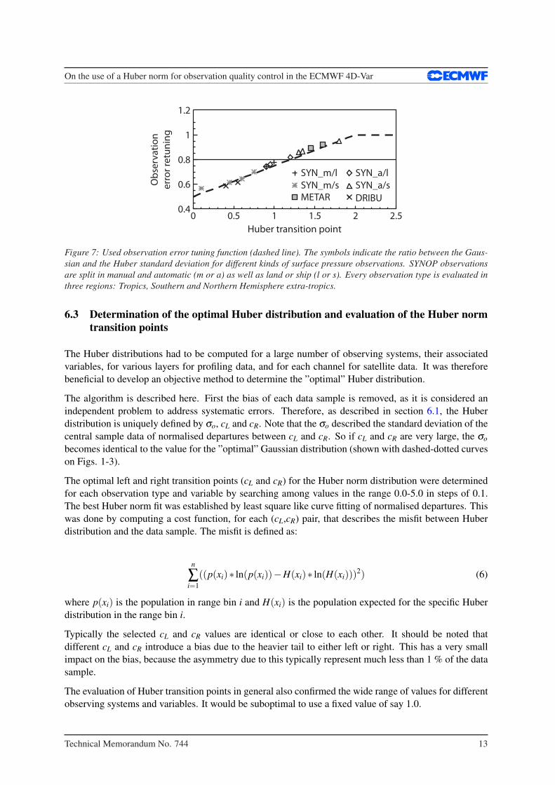
We examined this for all the observing systems for which a Huber norm distribution was applicable.The symbols on Figure 7 shows the ratio of the estimated σo for the optimal Huber norm distributionand the optimal value for a Gaussian distribution for a range of surface pressure observing systems.Values are plotted as function of the average Huber left and right transition points (cL and cR) for threedifferent areas: Northern Hemisphere extra-tropics, Tropics and Southern Hemisphere extra-tropics. Theselected observing systems cover a wide range of Huber transition points. It was found that on averagethe observation error is reduced to 80% of the previously used value. There is an approximately linearrelationship between the observation error retuning factor and the Huber norm transition point.

The retuning factor can be estimated well with the simple function defined in Eq. (5).

Tσo = Min[

1.0 , 0.5+0.25(

cL + cR

2

)](5)

Here Tσo is the retuning value for a certain observation. cL and cR are the right and left transition pointof the Huber distribution, respectively. We choose this simple linear function as it described the relationvery accurately (see the dashed curve on Figure 7). There was no justification for implementing a morecomplex or statistically based tuning function.



1.2

1

0.8

0.6

0.40 0.5 1

SYN_m/l

SYN_m/s

SYN_a/l

SYN_a/s

METAR DRIBU

Huber transition point

1.5 2 2.5

Ob

serv

ati

on

err

or

retu

nin

g

Figure 7: Used observation error tuning function (dashed line). The symbols indicate the ratio between the Gaus-sian and the Huber standard deviation for different kinds of surface pressure observations. SYNOP observationsare split in manual and automatic (m or a) as well as land or ship (l or s). Every observation type is evaluated inthree regions: Tropics, Southern and Northern Hemisphere extra-tropics.

6.3 Determination of the optimal Huber distribution and evaluation of the Huber normtransition points

The Huber distributions had to be computed for a large number of observing systems, their associatedvariables, for various layers for profiling data, and for each channel for satellite data. It was thereforebeneficial to develop an objective method to determine the ”optimal” Huber distribution.

The algorithm is described here. First the bias of each data sample is removed, as it is considered anindependent problem to address systematic errors. Therefore, as described in section 6.1, the Huberdistribution is uniquely defined by σo, cL and cR. Note that the σo described the standard deviation of thecentral sample data of normalised departures between cL and cR. So if cL and cR are very large, the σo

becomes identical to the value for the ”optimal” Gaussian distribution (shown with dashed-dotted curveson Figs. 1-3).

The optimal left and right transition points (cL and cR) for the Huber norm distribution were determinedfor each observation type and variable by searching among values in the range 0.0-5.0 in steps of 0.1.The best Huber norm fit was established by least square like curve fitting of normalised departures. Thiswas done by computing a cost function, for each (cL,cR) pair, that describes the misfit between Huberdistribution and the data sample. The misfit is defined as:

n

∑i=1

((p(xi)∗ ln(p(xi))−H(xi)∗ ln(H(xi)))2) (6)

where p(xi) is the population in range bin i and H(xi) is the population expected for the specific Huberdistribution in the range bin i.

Typically the selected cL and cR values are identical or close to each other. It should be noted thatdifferent cL and cR introduce a bias due to the heavier tail to either left or right. This has a very smallimpact on the bias, because the asymmetry due to this typically represent much less than 1 % of the datasample.

The evaluation of Huber transition points in general also confirmed the wide range of values for differentobserving systems and variables. It would be suboptimal to use a fixed value of say 1.0.



For profiling data the vertical distribution of the Huber left and right transition points were computed foreach 100hPa vertical level. Figure 8 shows an example of this for Vaisala RS92 radiosonde temperatures.Investigations showed that the Huber norm transition points tended to be distinct for three layers in theatmosphere: the stratosphere (observations above 100hPa), the free troposphere (observations between100hPa and 900hPa), and the boundary layer (observations below 900hPa). So Huber norm distributionswere computed and applied for these three layers for radiosonde, pilot, aircraft, and wind profiler data.Notice that the transition points shown in Figure 8 differ in the stratosphere for the left and right transi-tion point. This flexibility in the formulation gives us the opportunity to account for differences in thebehaviour of the negative/positive temperature departures. Because we use departure distributions forthe evaluation, it is not clear if the observations or the background fields are responsible for asymmetricbehaviour in the tails of the distribution. It could be questioned why the left and right transition pointfor radiosondes should change with height. It could possibly be linked to representativeness errors thatin ECMWF’s, and most other assimilation systems, are treated as part of the observation error. But inseveral cases we are able to link asymmetries of temperature departures to issues with the observingsystem. It is of course preferable to correct for systematic observation errors and model errors closer tothe source.

Huber transition point

Pre

ssu

re (

hP

a)

21.510.51000

100

10

Figure 8: Profile of the optimal left and right transition points for Vaisala RS92 radiosonde temperature data foreach 100hPa layer. Solid: Left transition point, dashed: right transition point.

6.4 Huber norm VarQC implementation at ECMWF

Further aspects that need to be considered when implementing the Huber norm VarQC in an operationalNWP system are discussed here using the ECMWF operational implementation as an example. BecauseHuber norm VarQC is a robust method, it allows the relaxation of the background QC. This is a veryimportant side benefit of the Huber norm method, because it makes observations with large departuresactive, so the data get a chance to influence the analysis. The observation errors were also adjusted asdiscussed in section 6.2.

The weights, W , are computed based on the high resolution departures in the non-linear outer loop ofthe incremental 4D-Var [Courtier et al. (1994)]. The weights are kept constant during the minimisation



(inner loop), because the Lanczos minimisation algorithm [Fisher et al. (2009)] used at ECMWF doesnot allow the function that is minimised to be modified during the minimisation process. Some minimi-sation methods are more lenient and would allow the weights to be adjusted slightly for each iteration ofthe minimisation process. But the benefit of the much faster, but strictly quadratic, Lanzcos algorithmoutweighs the benefit of a more dynamic QC. The weights are updated at each of the three relinearisationouter loops applied at ECMWF, this makes it possible for the analysis to change the weights during theassimilation cycle.

In this paper we concentrate our investigation on conventional observations. As mentioned in section 3.4,it is expected that the Huber norm QC will be most beneficial for conventional data. Of the conventionalobserving systems used in ECMWF’s assimilation system it was found that the distributions for thefollowing observation types and variables were very well represented by a Huber norm distribution:

• Radiosonde observations: temperature and wind upper air data (with special Huber norm distribu-tions fitted to dropsondes).

• Aircraft observations: temperature and wind upper air data.

• Pilot balloon observations: wind upper air data.

• Wind profiler observations: wind upper air data from American, European and Japanese windprofilers.

• Land surface observations: surface pressure data from automatic and manual synop reports.

• Ship observations: surface pressure and wind data from automatic and manual ship reports.

• Airport observations: surface pressure data from metar reports.

• Drifting and moored buoy observations: surface pressure and wind data from drifting and mooredbuoys.

So these observation types were all included in the operational analysis system update of the variationalQC. The remaining observation types and variables kept the ”Gaussian plus flat” distribution.

The Huber norm QC is not implemented for humidity in the present implementation at ECMWF due tothe difficulties discussed in section 3.3. It is planned to implement this in a forthcoming update.

6.5 Weights for Huber norm VarQC

Following the definition from AJ99 we define the probability of gross error, scaled to the range 0.0-1.0, tobe 1−W . The left panel of Figure 9 shows the distribution of gross error probabilities for the 18 monthssample of stratospheric radiosonde temperature data. The transparent black bars are for the previouslyused ”Gaussian plus flat” distribution and the grey shaded bars are for the Huber norm distribution. Notethe vertical scale is logarithmic and bars have a width of 0.01. It is seen that more than 99% (100,000)of the observations have gross error probabilities below 0.01. This is the case for both distributions. Inthe gross error probability range from 0.01 to 0.5 the Huber norm has similar data counts in each bin.For higher values the data counts fall off, because there are so few data values in the extremes of thedeparture distribution. For the ”Gaussian plus flat” distribution bin data counts are reduced between 0.01and 0.5, and reach a level that is an order of magnitude lower than for the Huber norm distribution at 0.5.



For higher gross error probabilities the data counts are increased for the ”Gaussian plus flat” distribution- a result of the sharp transition zone for gross error probabilities closer to the centre of the distribution,resulting in more observations with large probability of gross error values. The right panel of Figure9, similar to Figure 5b, shows the corresponding weights for the optimal Huber norm distribution andthe previously used ”Gaussian plus flat” distribution. It gives a qualitative understanding of the differentshape of data count bar charts for the gross error probabilities shown on the left panel.

100000

10000

1000

100

10

1

1.4 Huber left: 1.8Huber right: 1.5

Normalised background departures0–5–10 5 10

Gaussian weightsHuber weights1.2

1

0.8

We

igh

t

0.6

0.4

0.2

0

Probability of gross error

Da

ta c

ou

nt

0.1 0.2 0.3 0.4 0.5 0.6 0.7 0.8 0.9

Figure 9: Illustration of the VarQC weights for a Huber norm compared to a Gaussian and flat distribution.Left: Data count as a function of the probability of gross errors, right: corresponding weight functions for thetwo distributions. Huber values were taken from the radiosonde temperature observations in the stratosphere (≤100hPa).

6.6 Relaxation of the background quality control

Before the introduction of the Huber norm VarQC the background QC had rather strict limits. Typicalstandard deviation values (α) would be around five [Jarvinen and Unden (1997)] for the normalised de-partures, (o−b)2 < α2(σ2

o + σ2b ) , where σo and σb are the observation and background error standard

deviation, respectively. For the Huber norm VarQC this has been relaxed to around 15 standard devia-tions of the normalised innovation departure values. The ”BG QC limits” column in Table 1 in section7.1 shows the background QC values for the ”Gaussian plus flat” distribution (labelled Old) and for theHuber norm QC in details for all the involved observation types and variables. The values shown inTable 1 are absolute values in SI units. It could be argued that a background QC is not necessary anymore when a robust estimation in the variational QC is applied, but the relaxed limits are still helpful inrejecting clearly erroneous gross errors, like zero Kelvin temperatures.

7 General impact and case studies

The overall impact of the Huber norm implementation was evaluated over a three month data assimilationperiod in 2008 and for a number of intense weather events where the Huber norm implementation wouldbe expected to make the biggest difference. For all the experiments presented in this Section the onlydifference between the control assimilations and Huber norm assimilations are the quality control anderror distribution differences described in the paper.



7.1 A general summary of QC decisions for the Huber norm implementation

Table 1 shows shows the QC statistics for control (old) and Huber norm assimilations for all conventionalobservations that use the Huber norm quality control. The data is averaged for the period of 15 November2008 to 31 December 2008. Upper air observation statistics are split up into three vertical bins, asdescribed in section 6.3. The main differences are due to the relaxation of the background QC, theuse of a Huber norm fit to the departure statistics and the retuning of observation errors. The first datacolumn shows the total number of observations presented to the Huber norm assimilation and the controlassimilation are the same. The next two columns show the percentage of background rejected (labelledFG rej) data. The change in background rejections is clear for all observation types, with significantlyless rejections for the Huber norm assimilation experiment. Next follow columns showing percentageof data with very low variational QC weight (less than 25%). It is called VarQC rejected data, eventhough the data is not fully rejected. The data is still active data and influence the analysis accordingto its reduced weight. As discussed in section 6.5, the percentage of VarQC rejected data are generallylarger for the Huber norm because it is the percentage of a much larger sample that pass the backgroundQC. It is also related to the shape of the probability of gross error distributions, as shown in Figure 9.The final four columns show the approximate limits used by the different quality control decisions. Theterm ‘no data’ means that no data was background rejected for this data type during the six week periodevaluated. The VarQC limits show the range for which the weights get below 25%.

All obsObstype Value Level *1000 Ol d Huber Ol d Huber Ol d Huber Ol d Huber

SYNOP Ps surf 5373 0.58 0.19 0.11 0.42 260.0 780.0 200.0 140.0 PaSHIP Ps surf 360 0.94 0.17 0.97 2.56 280.0 1100.0 200.0 180.0 PaSHIP U/V surf 350 0.77 0.02 0.43 5.44 11.2 12.7 10.8 5.4 m/sDRIBU Ps surf 1156 1.17 0.55 0.47 0.97 360.0 800.0 200.0 200.0 PaDRIBU U/V surf 111 4.05 0.77 1.56 6.63 10.7 26.3 7.4 4.3 m/sMETAR Ps surf 2070 0.05 0.00 0.09 0.07 1000.0 >1600 340.0 80.0 PaTEMP T 0-100 693 0.96 0.04 2.03 0.15 5.2 29.0 3.6 6.6 KTEMP T 100-900 1614 0.54 0.02 0.66 0.70 3.3 15.8 2.5 2.5 KTEMP T 1000-900 188 0.88 0.03 1.45 4.33 5.1 21.8 3.6 2.6 KTEMP U/V 0-100 716 0.49 0.09 0.78 0.61 13.9 22.5 10.2 11.5 m/sTEMP U/V 100-900 1237 0.35 0.08 0.39 0.79 11.2 23.5 9.1 6.5 m/sTEMP U/V 1000-900 189 0.44 0.06 0.48 2.67 11.1 30.9 9.2 6.5 m/sAIREP T 100-900 8477 0.08 0.00 0.05 0.19 4.4 15.9 3.8 1.4 KAIREP T 1000-900 1529 0.40 0.03 0.09 1.77 6.2 23.9 5.0 1.5 KAIREP U/V 100-900 8483 0.09 0.02 0.08 0.28 ~15.0 ~21.5 12.7 9.1 m/sAIREP U/V 1000-900 1483 0.63 0.17 0.11 0.62 ~15.0 no data 12.5 8.9 m/sPILOT U/V 0-100 238 0.53 0.04 0.81 0.71 14.3 24.6 10.3 11.6 m/sPILOT U/V 100-900 536 0.39 0.04 0.61 1.27 11.6 23.4 9.2 6.5 m/sPILOT U/V 1000-900 100 0.32 0.03 0.32 2.20 11.5 51.4 9.2 6.5 m/sprofiler U/V 0-100 73 0.90 0.15 0.52 0.65 15.9 22.0 10.7 12.2 m/sprofiler U/V 100-900 4061 0.15 0.03 0.10 0.25 12.7 22.2 9.2 6.5 m/sprofiler U/V 1000-900 346 0.01 0.00 0.02 0.06 13.2 no data 9.2 6.5 m/sEU-profiler U/V 0-100 8 0.41 0.00 0.71 0.52 17.3 no data 10.7 12.4 m/sEU-profiler U/V 100-900 2036 0.08 0.02 0.06 0.13 12.7 24.2 9.2 6.5 m/sEU-profiler U/V 1000-900 246 0.01 0.00 0.02 0.08 13.2 no data 9.2 6.5 m/sJP-profiler U/V 100-900 303 0.18 0.01 0.49 0.85 13.2 22.2 9.2 8.4 m/sUS-profiler U/V 0-100 46 1.36 0.24 0.70 0.93 15.9 22.0 10.7 12.2 m/sUS-profiler U/V 100-900 1181 0.34 0.07 0.13 0.40 13.4 24.1 9.7 8.9 m/s

BG QC limits VarQC rej limits% FG rej % VarQC rej

Table 1: Data usage table showing the background QC and the VarQC rejections for 15 Nov 2008 - 31 Dec 2008of operational data (Old) and the Huber norm assimilation experiment (Huber). VarQC rejected is defined by aweight smaller than 25%. The count for all observations is in thousands and is the same for both datasets.

This change in variational QC was implemented into the operational forecasting system at ECMWF inSeptember 2009 [Tavolato and Isaksen (2010)] and has proven to have a positive impact on the use ofconventional observations within the assimilation system.



System Resolution lowest Ps (hPa)ERA-Interim T255 - T95,T159 978.0hPaHuber exp. T255 - T95,T159 976.9hPaHuber exp. T319 - T95,T159 976.4hPaHuber exp. T319 - T95,T255 975.6hPaHuber exp. T511 - T95,T255 974.3hPaObservation 962.4hPa

Table 2: The lowest observed and analysed surface pressures on 26 December 1999 0600 UTC. The lowest valueis a surface pressure observation. The Huber norm assimilation experiment deepens the low compared to ERA-Interim. A further improvement can be found when increasing the resolution (inner and outer loop).

A number of impact studies and general investigations have been performed to evaluate the impact ofthe Huber norm quality control. Assimilation experiments over a period of three months in 2008 showeda small positive impact over Europe and the Northern Hemisphere extra-tropics in general, and neutralscores for the Southern Hemisphere extra-tropics.

During the last week of December 1999 two small-scale lows affected Europe with intense gusts andstorm damage. These storms are ideal case studies due to the high-density, high-quality synoptic landstation surface pressure network over France and Germany. These surface pressure observations capturedthe intensity and location of the storms very well, and neighbouring stations consistently support eachother. However, the strength of these storms was poorly represented in both the operational ECMWFanalysis and the ERA-Interim [Dee et al. (2011)]. Both assimilation systems used the old (”Gaussianplus flat” distribution) QC method.

A number of case studies were performed to investigate the assimilation impact of applying the Hubernorm VarQC in the analysis system. The Huber norm experiments were run with the same model versionas ERA-Interim, for most experiments at the same resolution.

7.2 Lothar, 26.12.1999

The first of the December 1999 storms that hit Europe on 26 December 1999 is known as Lothar[Ulbrich et al. (2001)]. It followed a path from the Atlantic to France, moving eastwards into Germany.The position of this storm was well predicted in both analyses (ERA-Interim as well as the Huber normexperiment) but the intensity is not captured well in ERA-Interim. Indeed, the SYNOP observationsreporting the lowest surface pressure were background rejected in the ERA-Interim. The Huber normexperiment showed a reduced central pressure compared to the reanalysis because many more observa-tions were assimilated. However, the analysis was still significantly above the lowest observed surfacepressure. One of the reasons is that the analysis is not able to capture the small scale of this event wellenough at the reanalysis resolution.

To evaluate the influence of the resolution several Huber norm experiments with different resolutions(inner and outer loop) were carried out and the results are shown in Table 2. It shows that increasedresolution is beneficial.



1010

2

1

1722

0

68

25

48

50°N

1000

990

980

54

30

65

32

49

65

65

5247 64

40

61

74

71

5732

34 23 32

73

61

17

59

60

36

50

5730

73

62

57

1451

5517

39

29

56

1720

52

64

4938

35

62

35

68

59

3855 54

58

50

5715

1246

47

38

65

43

22

63

74

6043

67

3327

48

74

21

50

40

45 58

63

68

69

44

2750

26

7

7248

32

20

37

46

17

40

57

32

16

36

37

69

2473

46

4737

38

5571 29

3050

61 21

34

60 39

50°N

0°

0°

HL

HL

970

980

990

1000

1010

Figure 10: Rejections on 27 December 1999 1800 UTC, top: ERA-Interim, bottom: Huber norm experiment.The contours show the analysed surface pressure field for each experiment. Black triangles indicate backgroundrejected observations, numbers the effective VarQC weights for quality controlled stations. Grey circles indicateobservations with weights higher than 75%.

7.3 Martin, 27.12.1999

The second storm was the very intense Martin that reached the French coast on 27 December 1999[Ulbrich et al. (2001)]. It was poorly predicted, being too weak and misplaced in the operational ECMWFanalysis; ERA-Interim produced similar poor results. Most surface pressure observations near the cy-clone centre were rejected by the background quality control (shown as filled triangles on Figure 10 toppanel) even though a hand analysis showed that all the observations from France were correct. This ledto an analysis with the storm centre further to the east than surface pressure observations would suggest.The lowest surface pressure observation at 1800 UTC on 27 December 1999 reported 963.5hPa. It wasone of the background QC rejected observations in ERA-Interim.

The bottom panel of Figure 10 shows rejections and observation weights from the Huber norm assimi-lation experiment. The numbers show the QC-weight associated with each surface pressure observation:they are 16% or higher for all stations. More observations get higher QC-weights than in the reanalysisdue to the Huber norm. The centre of the low has correctly moved further to the west in good agreementwith the observations. Furthermore, the minimum surface pressure is reduced significantly.

The analysis and the observation rejections for the December 1999 storm cases have also been discussedby [Dee et al. (2001)]. They use an adaptive buddy check QC approach with the same effect as the Huber



norm method to analyse this case. However, the Huber norm method is simpler to implement in the IFS.

7.4 June 2008 extra-tropical event

At the beginning of June 2008 exceptionally low forecast scores were seen for the five day 500hPageopotential height forecast over Europe (anomaly correlation errors for 500hPa geopotential heightwere below zero) in several NWP models (not shown).

In the operational ECMWF system this drop in performance was linked to the rejection (mainly back-ground rejection) of radiosonde and aircraft observations around 200hPa over North America. Mostof the background rejected data had relatively small background departures, just outside the QC limits.Applying the Huber norm VarQC had the effect that all these observations were used and the five dayforecast improved drastically. Figure 11 shows the verifying analysis over Europe on 11 June 2008 (top)and the two five day forecasts (operational system in the middle, Huber norm experiment in the bottompanel). The westerly flow over Europe is predicted much better in the Huber norm VarQC experiment.

7.5 Tropical cyclones

The Huber norm QC and relaxation of rejection limits are also applied for dropsonde wind and tempera-ture observations. It results typically in more correctly analysed tropical cyclones.

Results for hurricane Ike, hurricane Bill and typhoon Hagupit from September 2008 (Ike, Hagupit) andAugust 2009 (Bill) are discussed here. The two Atlantic hurricanes were well observed by dropsondes.Usage statistics for this period confirms that more dropsonde wind and temperature data was used in theHuber norm experiment than in the operational system.

Figure 12 shows the observed cyclone track, marked with crosses for every six hours, and the anal-ysis of surface pressure for the three tropical cyclones at one selected analysis time during the mostintense cyclone phase. The gray contours show the mean-sea-level (MSL) pressure analysis. The blacksolid/dashed contours show the reduction/increase in MSL pressure when Huber norm QC and relaxedbackground error QC is applied. It is evident that all three tropical cyclones have been intensified verysignificantly by using the revised observation QC. Figure 13 shows the time series of core surface pres-sure every six hours. These results indicate that the use of the Huber norm (solid lines) intensified thecore pressure compared with the analysis that used the ”Gaussian plus flat” distribution (dashed line) inthe quality control for many analysis cycles during the intense phase of the tropical cyclones.

For the Atlantic hurricanes Ike and Bill measurements of the core MSL pressure is available (shown withthe dash-dotted lines on Figure 13). For storm Hagupit no core MSL pressure observations are available,but the intensity estimates for Hagupit indicates it developed into a typhoon from a tropical storm on 20Sep 2008. This means it was too weak in both analyses. So all three time series show that the Hubernorm experiment is improving the surface pressure analysis of the tropical cyclones.

It is clear that when extensive dropsonde data is available, like for hurricane Bill, deeper and moreaccurate analyses were obtained when the Huber norm quality control was applied.



L

L

LL

530540

550

570

570

570

560 550

540

580

560

590

H

H

L

H

H

L

L

550

550

560

580

580

590

59030°N

40°N

50°N

60°N

70°N

30°N

40°N

50°N

60°N

70°N

30°N

40°N

50°N

60°N

70°N

20°W 0° 20°E 40°E

20°W 0° 20°E 40°E

20°W 0° 20°E 40°E

H

L

L

Figure 11: Analysis for 500hPa geopotential height for 11 June 2008 (top panel) and the five-day forecast validat the same time from the operational ECMWF system (middle panel) and the Huber norm experiment (bottompanel).



H

L

1000

1010

30°N

a

b

c

20°N

80°W

120°E

990

1000

H

H

1010

1020

20°N

60°W

L

Figure 12: Improvement on tropical cyclone analyses due to Huber norm QC. One solid black contour indicates adifference of 1hPa (2hPa) in the surface pressure analysis in panel a and b (in panel c) compared to the control.Black crosses indicate the cyclone path. Panel a: Hurricane Ike on the 10 September 2008 1800 UTC in the Gulfof Mexico approaching Texas. Panel b: Typhoon 0814 Hagupit on the 21 September 2008 1800 UTC in the Pacificapproaching the Chinese coast. Panel c: Hurricane Bill on the 20 September 2009 0000 UTC in the CaribbeanOcean.



Hagupit – September 2008

Pre

ssu

re (

hP

a)

22212019960

970

980

990

1000

1010

Pre

ssu

re (

hP

a)

940

950

960

970

980

990

23 24

Bill – September 2009

Pre

ssu

re (

hP

a)

201918940

960970

950

980990

10001010

21 22

Ike – September 2008121110 13

Figure 13: Time series of tropical cyclone center surface pressure (in hPa) for the storms Ike (top), Hagupit(middle) and Bill (bottom). The solid line shows the surface pressure analysis from the Huber norm assimilationexperiment, the dashed curve is the control experiment. The dash-dotted line shows the observed surface pressureif available. The grey shaded area indicates the time after the land fall of the cyclone and the vertical line marksthe date and time used in Figure 12.

8 Conclusions

The paper describes a number of aspects that are important to consider for quality control (QC) of ob-servation used in data assimilation systems. Observations have measurement errors, representativenesserrors and sometimes gross errors. In data assimilation innovations are used extensively for observationQC and provide generally very valuable information [Hollingsworth et al. (1986)]. But the backgroundforecasts also have errors, sometimes very large ones, so it may be difficult to determine if an observa-tion or the equivalent model value is the outlier. Monitoring time series for individual in-situ stations andsatellite channels provide a powerful method for detecting poorly performing or erratic platforms. It isshown how semi-logarithmic plots of normalised departures also are able to identify groups of outliers.Studying these outlier samples makes it often possible to identify problems with observations used inthe data assimilation system, e.g., due to representativeness errors in mountainous areas. For humiditydata normalisation is required to obtain Gaussian-like innovations. For satellite data clouds, rain andsurface emissivity may contaminate the atmospheric signal. The semi-logarithmic plots of normaliseddepartures also provide useful guidance in detecting this. A comprehensive evaluation was performed ofthe departure statistics for every observing system and every variable used in the ECMWF assimilationsystem over an 18 month period. After filtering out systematic outliers (”blacklisting” of stations andsatellite channels) there is very little evidence of gross errors for the observations used in the departuredistributions. This is likely because most observations now are automated and therefore either of nominalquality or all represent gross errors that therefore are easy to detect.



The difficulties related to assimilation of isolated frequently reporting stations with biases is discussed.It is shown how important it is to do bias correction of isolated stations, especially when observation QClimits are relaxed. It is important to consider this when an observation QC scheme is developed.

Various QC methods for handling outliers are presented. The main issue is how much weight to assign tooutliers. The ”Gaussian plus flat” distribution method [Andersson and Jarvinen(1999)] used at ECMWFfrom 1999 to 2009, had fairly strict background QC limits and a sharp transition from observations beingactive to being given virtually no weight in the analysis. The paper describes the introduction of a Hubernorm QC that makes it safe to use observations with large departures in the analysis. This is becauseit is a robust method where the moments of the distribution are affected very little by a few erroneousoutliers.

Evaluating the 18 months innovation data sample from ECMWF showed that almost all departure dis-tributions were well described by the Huber norm distribution, after removing systematically erroneousdata. The fit was much better than for the pure Gaussian distribution or a ”Gaussian plus flat” distribution.It was also shown to be beneficial to introduce the flexibility of allowing different left and right transitionpoints from the Gaussian to exponential part of the Huber distribution. It is acknowledged that a Huberdistribution fit for the normalised innovations does not prove that the observation error distribution fol-lows a Huber distribution. Innovation distributions are a convolution of observation and background errordistributions. For the background QC it is theoretically correct to use the innovation statistics, but for theobservation cost function term it is not. But it is shown that it is more beneficial to relax the observationQC and allow outliers to influence the analysis under the assumption that observation errors follow therobust Huber distribution. Several case studies show how the Huber norm quality control deserves thecredit for improved analyses and forecasts of extreme events such as extra-tropical storms and tropicalcyclones. The examples show the strength of the robust Huber norm approach that enables the analysisto benefit from observation outliers in the situations when several observations deviate significantly andconsistently from the model background. The previously used quality control method would reject suchobservations.

The Huber norm quality control has been implemented successfully at ECMWF in September 2009 forwind, temperature and surface pressure measurements from all conventional observations available. Inthe future this will be extended to humidity and some satellite data.

This work has also shown that refined quality control and observation error tuning can be an importantmethod to help extract more information from observations. It is an area of data assimilation where thereis potential for further improvements.

Acknowledgements

The authors want to thank Hans Hersbach (ECMWF) for providing the software to compute the best fitHuber distribution. Elias Holm and Erik Andersson, both ECMWF staff, provided helpful comments.We thank Rob Hine and Anabel Bowen, ECMWF staff, for improving our figures significantly. Partof this work has been funded by project P21772-N22 of the Austrian Fonds zur Forderung der wis-senschaftlichen Forschung (FWF).



References

[Andersson et al. (2005)] Andersson E., Bauer P., Beljaars A., Chevallier F., Holm E.,Janiskova M.,Kallberg P., Kelly G., Lopez P., McNally A., Moreau E., Simmons A. J., Thepaut J.-N. and Tomp-kins A. M. 2005. Assimilation and Modeling of the Atmospheric Hydrological Cycle in the ECMWFForecasting System, Bull. Am. Meteorol. Soc., 86(3):387-403.

[Andersson and Jarvinen(1999)] Andersson E., and Jarvinen, H. 1999 Variational quality control, Quart.J. Roy. Meteor. Soc., 125:697-722.

[Bonavita et al. (2012)] Bonavita, M., Isaksen, L. and Holm, E. 2012. On the use of EDA backgrounderror variances in the ECMWF 4D-Var. Q.J.R. Meteorol. Soc. doi: 10.1002/qj.1899

[Courtier et al. (1994)] Courtier P., Thepaut J.-N. and Hollingsworth A. 1994. A strategy for operationalimplementation of 4D-Var, using an incremental approach, Quart. J. Roy. Meteor. Soc., 120:1367-1388.

[Courtier et al. (1998)] Courtier, P., Andersson, E., Heckley, W., Vasiljevic, D., Hamrud, M.,Hollingsworth, A., Rabier, F., Fisher, M. and Pailleux, J. 1998. The ECMWF implementation ofthree-dimensional variational assimilation (3D-Var). I: Formulation., Quart. J. Roy. Meteor. Soc.,124:1783-1807.

[Dee et al. (2001)] Dee D. P., Rukhovets L., Todling R., da Silva A. M. and Larson J.W. 2001. An adap-tive buddy check for observational quality control, Quart. J. Roy. Meteor. Soc., 127:2451-2471.

[Dee et al. (2011)] Dee D. P., Uppala S. M., Simmons A. J., Berrisford P., Poli P., Kobayashi S., AndraeU., Balmaseda M. A., Balsamo G., Bauer P., Bechtold P., Beljaars A. C. M., van de Berg L.,Bidlot J., Bormann N., Delsol C., Dragani R., Fuentes M., Geer A. J., Haimberger L., Healy S.B., Hersbach H., Holm E. V., Isaksen L., Kallberg P., Kohler M., Matricardi M., McNally A. P.,Monge-Sanz B. M., Morcrette J.-J., Park B.-K., Peubey C., de Rosnay P., Tavolato C., ThepautJ.-N. and Vitart F. 2011. The ERA-Interim: configuration and performance of the data assimilationsystem, Quart. J. Roy. Meteor. Soc., 137:553-397.

[Desroziers et al. (2005)] Desroziers G., Berre L., Chapnik B. and Poli P. 2005. Diagnosis of observa-tion, background and analysis-error statistics in observation space, Quart. J. Roy. Meteor. Soc.,131:3385-3396.

[Dharssi et al. (1992)] Dharssi, I., Lorenc, A. C. and Ingleby, N. B. 1992. Treatment of gross errorsusing probability theory, Quart. J. Roy. Meteor. Soc., 118:1017-1036.

[Fisher et al. (2009)] Fisher M., Nocedal, J., Tremolet, Y. and Wright, S.J. 2009. Data assimilation inweather forecasting: a case study in PDE-constrained optimization, Optim. Eng. (2009),, 409-426.

[Guitton and Symes (2003)] Guitton A. and Symes W. W. 2003. Robust inversion of siesmic data usingthe Huber norm, Geophysics, 68(4):1310-1319.

[Hollingsworth et al. (1986)] Hollingsworth A., Shaw D. B., Lonnberg P., Illari, L., Arpe K. and Sim-mons A. 1986. Monitoring of observations and analysis quality by a data assimilation system, Mon.Weather Rev., 114:861-879.

[Holm et al. (2002)] Holm E., Andersson E., Beljaars A., Lopez P., Mahfouf J.-F., Simmons A. J. andThepaut J.-N. 2002. Assimilation and modelling of the hydrological cycle: ECMWF’s status andplans., Technical Memorandum, ECMWF, 383.



[Huber (1964)] Huber P. J. 1964. Robust estimates of a location parameter, Ann. Math. Statist., 35:73-101.

[Huber (1972)] Huber P. J. 1972. Robust statistics: a review, Ann. Math. Statist., 43(4):1041-1067.

[Huber (2002)] Huber P. J. 2002. John W. Tukey’s Contribution to robust statistics, The Annals of Statis-tics, 30(6):1640-1648.

[Ingleby and Lorenc (1993)] Ingleby N. B. and Lorenc A. C. 1993. Bayesian quality control using mul-tivariate normal distributions, Quart. J. Roy. Meteor. Soc., 119:1195-1225.

[Isaksen et al. (2010)] Isaksen, L., Bonavita, M., Buizza, R., Fisher, M., Haseler, J., Leutbecher, M. andRaynaud, L. 2010. Ensemble of data assimilations at ECMWF, TD technical Memorandum No.636. Available at www.ecmwf.int/publications/

[Jarvinen et al. (1999)] Jarvinen H., Andersson E. and Bouttier F. 1999. Variational assimilation of timesequences of surface observations with serially correlated errors, Tellus, 51A:469-488.

[Jarvinen and Unden (1997)] Jarvinen H. and Unden P. 1997. Observation screening and backgroundquality control in the ECMWF 3D Var data assimilation system, Technical Memorandum,ECMWF, 236.

[Lorenc (1984)] Lorenc A. C. 1984. Analysis methods for the qality control of observations, pp397-428 in Proceedings of ECMWF workshop on the use and quality control of meteorolog-ical observations for numerical weather prediction, 6-9 Nov. 1984. Available from ECMWF(/www/ecmwf.int/publications).

[Lorenc (1986)] Lorenc A.C. 1986. Analysis methods for numerical weather prediction, Quart. J. Roy.Meteor. Soc., 112:1177-1194.

[Lorenc and Hammon (1988)] Lorenc A. C. and Hammon O. 1988. Objective quality control of obser-vations using Bayesian methods - Theory, and practical implementation, Quart. J. Roy. Meteor.Soc., 114:515-543.

[Tavolato and Isaksen (2010)] Tavolato C. and Isaksen L. 2010. Huber norm quality control in the IFS,ECMWF Newsletter, 122:27-31.

[Tukey (1960)] Tukey, J. W. 1960. A survey of sampling from contaminated distributions., In Contribu-tions to Probability and Statistics, eds I. Olkin, S. Ghurye, W. Hoeffding, W. Madow and H. Mann,pp. 448-485. Stanford: Stanford University Press.

[Ulbrich et al. (2001)] Ulbrich, U., Fink, A. H., Klawa, M. and Pinto, J. G. 2001. Three extreme stormsover Europe in December 1999, Weather, 56(2001), 70-80.

[Vasiljevic et al. (2006)] Vasiljevic D., Andersson E., Isaksen L. and Garcia-Mendez A. 2006. Surfacepressure bias correction in data assimilation, ECMWF Newsletter, 108:20-27.


Christina Tavolato and Lars Isaksen Research Department · 744 On the use of a Huber norm for...

Documents

Transcript of Christina Tavolato and Lars Isaksen Research Department · 744 On the use of a Huber norm for...