Childless Aristocrats. Fertility, Inheritance, and ... · Childless Aristocrats. Fertility,...
36
Childless Aristocrats. Fertility, Inheritance, and Persistent Inequality in Britain (1550 – 1950) Paula Gobbi 1 Marc Go˜ ni 2 1 Universit´ e catholique de Louvain 2 University of Vienna
Transcript of Childless Aristocrats. Fertility, Inheritance, and ... · Childless Aristocrats. Fertility,...

Childless Aristocrats. Fertility, Inheritance, andPersistent Inequality in Britain (1550 – 1950)
Paula Gobbi1 Marc Goni2
1Universite catholique de Louvain
2University of Vienna
Motivation
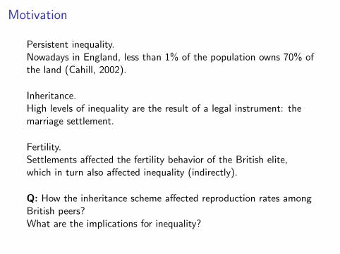
Persistent inequality.Nowadays in England, less than 1% of the population owns 70% ofthe land (Cahill, 2002).
Inheritance.High levels of inequality are the result of a legal instrument: themarriage settlement.
Fertility.Settlements affected the fertility behavior of the British elite,which in turn also affected inequality (indirectly).
Q: How the inheritance scheme affected reproduction rates amongBritish peers?What are the implications for inequality?
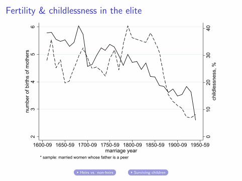
Fertility & childlessness in the elite
010
2030
40ch
ildle
ssne
ss, %
23
45
6nu
mbe
r of b
irths
of m
othe
rs
1600-09 1650-59 1700-09 1750-59 1800-09 1850-59 1900-09 1950-59marriage year
* sample: married women whose father is a peer
Heirs vs. non-heirs Surviving children

Inheritance
Heirs received all the land, younger brothers and sisters received anallowance
Marriage settlements
I Signed upon the marriage of the heir
I The heir committed to pass the estate unbroken to the nextgeneration in exchange for an anticipation
I De facto entailment
I Settled dowries and allowances
This paper
Estimate the effect of marriage settlements on childlessnessexploiting the demographic aspect of settlements.
Rationalize the link between inheritance, fertility, and wealthinequality.

Literature
1. Historical demographyI Malthus (1798); Chesnais (1992); Clark and Cummins (2009);
Goni (2015)
2. Fertility and inequalityI Number of children: Becker (1960); Heckman and Walker
(1990); De la Croix and Doepke (2003); Adsera (2005);Dettling and Kearney (2014)
I Childlessness: Aaronson, Lange, and Mazumder (2014);Baudin, de la Croix, and Gobbi (2015)
3. Inheritance and inequalityI Habakkuk (1950); Chu (1991); Engerman and Sokoloff (2000);
Bertochi (2006); Piketty and Saez (2006); Acemoglu (2008);Allen (2009); Long and Ferrie (2013); Clark and Cummins(2015).
Road map
1. Introduction
2. Data – Hollingsworth’s dataset
3. Empirical analysis
4. Theory
5. Summary

source: Cokayne’s Complete Peerage (1913)

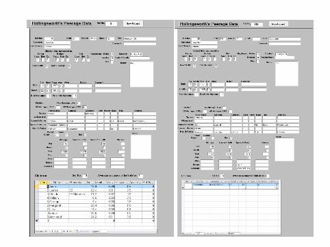

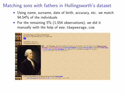
Matching sons with fathers in Hollingsworth’s dataset
I Using name, surname, date of birth, accuracy, etc. we match94.54% of the individuals
I For the remaining 5% (1,554 observations), we did itmanually with the help of www.thepeerage.com
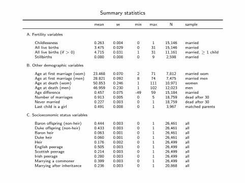
Summary statistics
mean se min max N sample
A. Fertility variables
Childlessness 0.263 0.004 0 1 15,146 marriedAll live births 3.475 0.029 0 31 15,146 marriedAll live births (if > 0) 4.715 0.031 1 31 11,161 married, ≥ 1 childStillbirths 0.080 0.008 0 9 2,598 married
B. Other demographic variables
Age at first marriage (wom) 23.468 0.070 2 71 7,812 married womAge at first marriage (men) 28.821 0.092 8 74 7,475 married menAge at death (wom) 50.853 0.246 1 111 10,971 womenAge at death (men) 46.959 0.230 1 102 12,023 menAge difference 0.457 0.075 -49 59 15,184 marriedNumber of marriages 0.913 0.005 0 5 18,759 dead after 30Never married 0.227 0.003 0 1 18,759 dead after 30Last child is a girl 0.491 0.008 0 1 3,967 matched parents
C. Socioeconomic status variables
Baron offspring (non-heir) 0.444 0.003 0 1 26,461 allDuke offspring (non-heir) 0.433 0.003 0 1 26,461 allBaron heir 0.063 0.001 0 1 26,461 allDuke heir 0.060 0.001 0 1 26,461 allHeir 0.176 0.002 0 1 26,499 allEnglish peerage 0.505 0.003 0 1 26,499 allScottish peerage 0.214 0.003 0 1 26,499 allIrish peerage 0.280 0.003 0 1 26,499 allMarrying a commoner 0.399 0.003 0 1 26,499 allMarrying after inheritance 0.236 0.003 0 1 20,868 all
Road map
1. Introduction
2. Data – Hollingsworth’s dataset
3. Empirical analysis
4. Theory
5. Summary
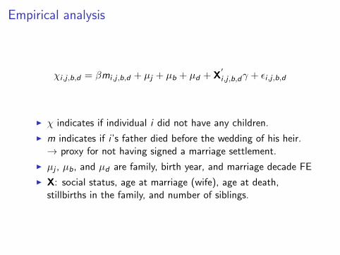
Empirical analysis
χi ,j ,b,d = βmi ,j ,b,d + µj + µb + µd + X′i ,j ,b,dγ + εi ,j ,b,d
I χ indicates if individual i did not have any children.
I m indicates if i ’s father died before the wedding of his heir.→ proxy for not having signed a marriage settlement.
I µj , µb, and µd are family, birth year, and marriage decade FE
I X: social status, age at marriage (wife), age at death,stillbirths in the family, and number of siblings.

Dep. variable: Childlessness (1650-1882)
non-heirs’ peers’heirs’ wives wives dau.
(1) (2) (3) (4) (5) (6)
Marrying after inheritance 0.047** 0.051*** 0.040** 0.077** 0.054 -0.000(0.019) (0.019) (0.018) (0.038) (0.070) (0.033)
Husband’s siblings (#) -0.001 -0.001 -0.001 -0.006 -0.007 -0.001(0.002) (0.002) (0.002) (0.005) (0.009) (0.004)
Father-in-law is a duke 0.022 0.025 -0.034 0.013(0.019) (0.019) (0.053) (0.110)
Wife’s age at marriage 0.015*** 0.014*** 0.016*** 0.021***(0.002) (0.004) (0.005) (0.003)
Wife’s age at death 0.000 -0.000 -0.001 -0.002**(0.000) (0.001) (0.001) (0.001)
Husband’s age at death -0.003*** -0.004*** -0.002 -0.001*(0.001) (0.001) (0.002) (0.001)
Still to live births (fam) 0.189 1.600** -20.514* -10.825***(0.315) (0.785) (11.686) (3.263)
Social status NO YES YES YES YES YESFamily FE NO NO NO YES YES YESBirth year FE NO NO NO YES YES YESMarriage decade FE NO NO NO YES YES YES
Observations 1,525 1,524 1,438 1,438 1,060 2,475Adjusted R2 0.003 0.014 0.059 0.021 0.082 0.170
Standard errors clustered by family in parentheses; *** p<0.01, ** p<0.05, * p<0.1.
births Scotland
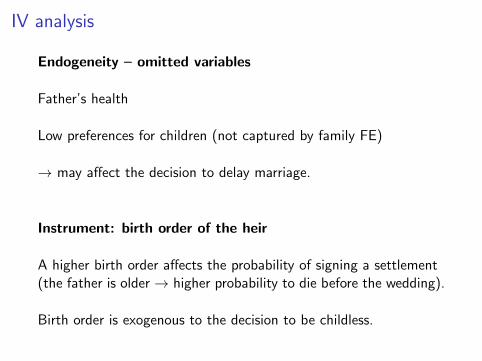
IV analysis
Endogeneity – omitted variables
Father’s health
Low preferences for children (not captured by family FE)
→ may affect the decision to delay marriage.
Instrument: birth order of the heir
A higher birth order affects the probability of signing a settlement(the father is older → higher probability to die before the wedding).
Birth order is exogenous to the decision to be childless.

First stage:
mi ,j ,b,m =15∑n=2
βnI(ri ,j ,b,m = n) + βzZi ,d + µd + X′i ,j ,b,mγ + εi ,j ,b,m
I ri ,j ,b,d is the birth order of individual i .
I µd are marriage decade fixed effects.
I X: social status, age at marriage (wife), age at death, andstillbirths in the family.
Second stage:
χi ,j ,b,d = βmi ,j ,b,d + µj + µb + µd + X′i ,j ,b,dγ + εi ,j ,b,d
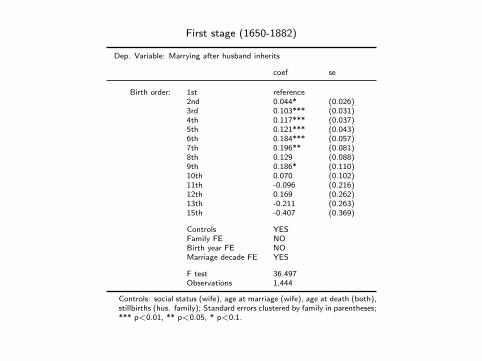
First stage (1650-1882)
Dep. Variable: Marrying after husband inherits
coef se
Birth order: 1st reference2nd 0.044* (0.026)3rd 0.103*** (0.031)4th 0.117*** (0.037)5th 0.121*** (0.043)6th 0.184*** (0.057)7th 0.196** (0.081)8th 0.129 (0.088)9th 0.186* (0.110)10th 0.070 (0.102)11th -0.096 (0.216)12th 0.169 (0.262)13th -0.211 (0.263)15th -0.407 (0.369)
Controls YESFamily FE NOBirth year FE NOMarriage decade FE YES
F test 36.497Observations 1,444
Controls: social status (wife), age at marriage (wife), age at death (both),stillbirths (hus. family); Standard errors clustered by family in parentheses;*** p<0.01, ** p<0.05, * p<0.1.
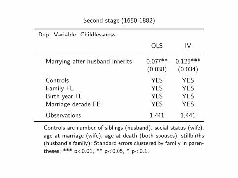
Second stage (1650-1882)
Dep. Variable: Childlessness
OLS IV
Marrying after husband inherits 0.077** 0.125***(0.038) (0.034)
Controls YES YESFamily FE YES YESBirth year FE YES YESMarriage decade FE YES YES
Observations 1,441 1,441
Controls are number of siblings (husband), social status (wife),
age at marriage (wife), age at death (both spouses), stillbirths
(husband’s family); Standard errors clustered by family in paren-
theses; *** p<0.01, ** p<0.05, * p<0.1.

Road map
1. Introduction
2. Data – Hollingsworth’s dataset
3. Empirical analysis
4. Theory
5. Summary

Set up
Unitary household decision model, utility:
u(c , L1, L2) = ln c+ln(ν+n)+βδ(m0) ln
(L1
L0
)+β2δ(me
1) ln
(L2
L0
)where
m =
{1 if at least one child is male0 otherwise.
Budget constraint:
c = r(1− λ0)L0 + pλ0L0 − qn − α(1− λ0)L0

Marriage settlement
Formally, the legal framework is:
λ0 = λ if M0 = 0λ0 = 0 if M0 = 1λ1 = λ and α = 0 if M1 = 0λ1 = 0 and α = α if M1 = 1
which implies the following dynamics
L1 = (1− λ0)L0 and L2 = (1− λ1)L1
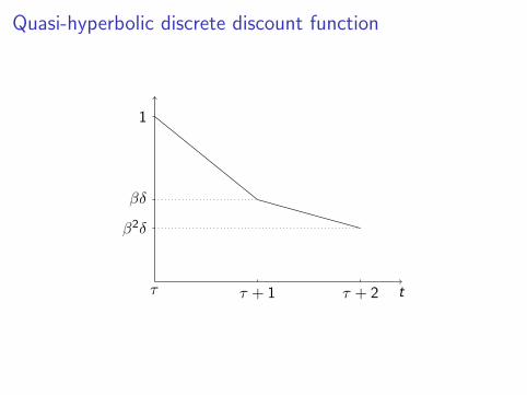
Quasi-hyperbolic discrete discount function
t
1
βδ
β2δ
τ τ + 1 τ + 2
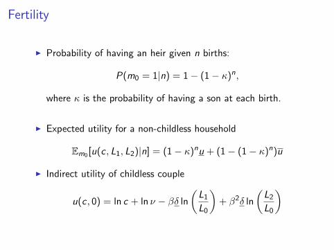
Fertility
I Probability of having an heir given n births:
P(m0 = 1|n) = 1− (1− κ)n,
where κ is the probability of having a son at each birth.
I Expected utility for a non-childless household
Em0 [u(c , L1, L2)|n] = (1− κ)nu + (1− (1− κ)n)u
I Indirect utility of childless couple
u(c , 0) = ln c + ln ν − βδ ln
(L1
L0
)+ β2δ ln
(L2
L0
)
Decisions
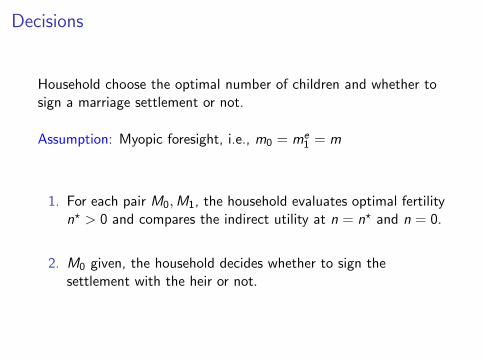
Household choose the optimal number of children and whether tosign a marriage settlement or not.
Assumption: Myopic foresight, i.e., m0 = me1 = m
1. For each pair M0,M1, the household evaluates optimal fertilityn? > 0 and compares the indirect utility at n = n? and n = 0.
2. M0 given, the household decides whether to sign thesettlement with the heir or not.
Numerical example
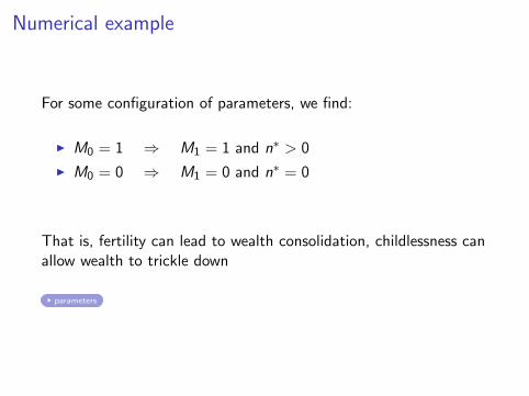
For some configuration of parameters, we find:
I M0 = 1 ⇒ M1 = 1 and n∗ > 0
I M0 = 0 ⇒ M1 = 0 and n∗ = 0
That is, fertility can lead to wealth consolidation, childlessness canallow wealth to trickle down
parameters

Road map
1. Introduction
2. Data – Hollingsworth’s dataset
3. Empirical analysis
4. Theory
5. Summary
Summary
In the absence of a marriage settlement, heirs were 10 percentagepoints more likely to be childlessness
Model rationalizes the relation between inheritance, fertility, andinequality
The rich get richer and the poor get—children!
The Great Gatsby

Back up slides

Fertility in the elite
010
2030
40%
23
45
67
num
ber
of b
irths
1600
-09
1650
-59
1700
-09
1750
-59
1800
-09
1850
-59
1900
-09
1950
-59
marriage year
births (average)childless (%)
* sample: married women whose husband is heir to a peerage
Heirs' wives
010
2030
40%
23
45
67
num
ber
of b
irths
1600
-09
1650
-59
1700
-09
1750
-59
1800
-09
1850
-59
1900
-09
1950
-59
marriage year
births (average)childless (%)
* sample: married women whose husband is a peers' non-heir son
Non-heirs' wives
more

Childlessness in the elite
010
2030
40%
23
45
67
num
ber
of b
irths
1600
-09
1650
-59
1700
-09
1750
-59
1800
-09
1850
-59
1900
-09
1950
-59
marriage year
births (average)childless (%)
* sample: married women whose husband is heir to a peerage
Heirs' wives
010
2030
40%
23
45
67
num
ber
of b
irths
1600
-09
1650
-59
1700
-09
1750
-59
1800
-09
1850
-59
1900
-09
1950
-59
marriage year
births (average)childless (%)
* sample: married women whose husband is a peers' non-heir son
Non-heirs' wives
back
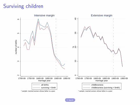
Surviving children
23
45
6nu
mbe
r of
birt
hs
1700-09 1750-59 1800-09 1850-59 1900-09 1950-59marriage year
all birthssurviving > 6mth
* sample: married women whose father is a peer
Intensive margin
010
2030
40%
1700-09 1750-59 1800-09 1850-59 1900-09 1950-59marriage year
childlessnesschildlessness (surviving < 6mth)
* sample: married women whose father is a peer
Extensive margin
back

Dep. variable: All live births of mothers (1650-1882) (poisson)
non-heirs’ peers’heirs’ wives wives dau.
(1) (2) (3) (4) (5) (6)
Marrying afterinheritance -0.033 -0.034 -0.012 -0.043 0.131* -0.023
(0.035) (0.035) (0.034) (0.046) (0.069) (0.044)
Siblings (hus.) 0.011** 0.011** 0.010** -0.012* -0.009 0.003(0.005) (0.004) (0.004) (0.006) (0.010) (0.004)
Controls NO YES YES YES YES YESFamily FE NO NO NO YES YES YESBirth year FE NO NO NO YES YES YESMarr. dec. FE NO NO NO YES YES YES
Observations 1,263 1,262 1,203 1,203 839 1,759
Controls are social status (wife), age at marriage (wife), age at death (both spouses),stillbirths (husband’s family); Standard errors clustered by family in parentheses.*** p<0.01, ** p<0.05, * p<0.1.
back

Dep. variable: Childlessness (1650-1882)
heirs’ wives
without Scotland only Scotland
Marrying after inheritance 0.130** -0.324(0.060) (0.483)
Husband’s siblings (#) -0.002 -0.047(0.006) (0.055)
Father-in-law is a duke 0.016 -0.036(0.022) (0.076)
Wife’s age at marriage 0.011** 0.066(0.005) (0.047)
Wife’s age at death 0.000 -0.016(0.001) (0.014)
Husband’s age at death -0.004** 0.003(0.002) (0.014)
Still to live births (fam) 1.514* 135.820(0.824) (146.599)
Social status YES YESFamily FE YES YESBirth year FE YES YESMarriage decade FE YES YES
Observations 1,089 249Adjusted R2 0.095 0.304
Standard errors clustered by family in parentheses; *** p<0.01, **p<0.05, * p<0.1.
back
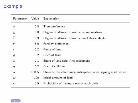
Example
Parameter Value Explanation
β 0.8 Time preference
δ 0.0 Degree of altruism towards distant relatives
δ 0.9 Degree of altruism towards direct descendants
ν 5.0 Fertility preference
r 0.2 Rents of land
p 0.2 Price of land
λ 0.1 Share of land sold if no settlement
q 0.2 Cost of children
α 0.005 Share of the inheritance anticipated when signing a settlement
L0 100 Initial amount of land
κ 0.5 Probability of having a son at each birth
back