MANUAL FOR ChE 496

CHEMICAL ENGINEERING LABORATORY II

Robert B. Barat

OTTO H. YORK DEPARTMENT OF CHEMICAL, BIOLOGICAL,

AND PHARMACEUTICAL ENGINEERING

NEW JERSEY INSTITUTE OF TECHNOLOGY NEWARK, NEW JERSEY 07102

Spring 2011 – Version 2

2

ACKNOWLEDGEMENT The author acknowledges that some material in this manual has been drawn from previous manuals used in the Chemical Engineering Laboratory courses at NJIT and produced by several contributors and authors. This author is grateful for this material. Copies of this current electronic manual are given to the students at no charge. It is available at: http://web.njit.edu/~barat UPDATES Updates of this manual are issued as needed, and are found online: http://web.njit.edu/~barat TABLE OF CONTENTS Page # AUTHOR’S NOTES 3 MODELING YOUR DATA 4 SUCCESSFUL PLANNING FOR EXPERIMENTS 7 SAFETY RULES AND REGULATIONS 8 LABORATORY REPORTING FORMATS 10 TUBULAR FLOW REACTOR 17 SEMI-BATCH REACTOR 25 LIQUID LEVEL CONTROL #1 33 GAS ABSORPTION IN A PACKED COLUMN 45 LIQUID LEVEL CONTROL #2 54 LIQUID-LIQUID EXTRACTION IN A KARR COLUMN 67 OPTICAL METHODS WITH BATCH REACTOR 74 CONTINUOUS DISTILLATION 80 CONTINUOUS STIRRED TANK REACTOR 94 TEMPERATURE CONTROL 100 PROTEIN OXIDATION IN A FLOW REACTOR 116

3

AUTHOR’S NOTES

• This manual is a work in progress, and will be updated as needed. Upgrades and other modifications will be done over time in order to improve our laboratory. Please be patient as the manual and our lab evolve over time.

• These experiments are based on concepts covered in most unit operations and

reactor engineering texts. The following references are especially useful:

1) Geankoplis, Transport Processes and Separation Process Principles, Prentice-Hall. 2) McCabe, Smith, and Harriot, Unit Operations of Chemical Engineering,

McGraw-Hill. 3) Foust, et al, Principles of Unit Operations, Wiley. 4) Fogler, Elements of Chemical Reaction Engineering, Prentice-Hall. 5) Perry’s Chemical Engineers Handbook.

4

MODELING YOUR DATA Philosophy In this course, you will use critical thinking in every stage of your laboratory work: Planning, Execution, Analysis, and Communication. This course should not be looked at as merely a "verification" of your prior lecture classes. Rather, it is a research activity to which you bring to bear all of what you've learned. Modeling A very important component of your Analysis is Modeling. As shown in the figure, the interaction between your experimental data and your model is a two-way path that will lead to the truth behind what you've done. You must have confidence in both your data and your model in order to be successful.

Exper iment

Model

T ru th

The choice of model is not a trivial one. Consider the following model classification: Fully Predictive

• Based on fundamental principles and assumptions • Might include parameters determined by previous researchers • User-input of experimental independent variables (e.g. flow rate set by you) • No adjustable parameters; predict dependent variables • Direct comparison of model predictions with observed data (e.g. outlet temperatures) • If comparison poor, review applicability of the model and/or data quality

Partially Predictive

• Based on fundamental principles and assumptions • User-input of experimental independent and dependent variables • Key parameter(s) determined by regression of observed data as applied through

the model equation(s) (e.g. heat transfer coefficient) • If regression not statistically acceptable, review applicability of the model and/or

data quality • If regression acceptable, compare values of fitted (regressed) parameters with

published or reasonable values

5

Simple Correlation

* Basis in fundamental principles and assumptions not needed * User-input of experimental independent and dependent variables into simple

regression (correlation) * If regression not statistically acceptable, correlation not valid * Acceptable regression suggests a relationship might exit, but is no guarantee

During data analysis, often there is confusion in applying which model type. We will not be using any simple correlations. The Fully Predictive model is always preferred. Many of the experiments have multiple parts, however, where you will require the Fully Predictive model for one part and the Partially Predictive model for another part. The choice depends on the availability of key modeling information. Example Consider the "Continuous Heat Transfer" Experiment. For the shell & tube steam condenser, you record condensate and coolant exit temperatures as functions of coolant rate for a given steam rate. Below, the various models are considered. Simple Correlation For a given steam flow rate, you observe that the exit coolant temperature changes as you vary its flow rate. You plot up this exit temperature vs. flow rate. By itself, this says little; you proceed to next level of complexity. Partially Predictive Your model includes the following components:

* Overall exchanger heat balance in terms of log-mean temperature driving force

and overall heat transfer coefficient. * Overall exchanger heat balances in terms of sensible heat gained by the cooling

water * Overall heat transfer coefficient as sum of resistances - incorporating both film

coefficients * Use both heat balances to estimate the overall heat transfer coefficient * Apply Wilson method to estimate the lumped quantity of tube metal resistance

and shell-side resistance * From sum of resistances, estimate tube-side heat transfer coefficient * Compare this tube-side coefficient to that predicted by literature correlation of

Nusselt numbers vs. Reynolds and Prantdl numbers Fully Predictive Your model includes the following components:

6

* Overall exchanger heat balance in terms of log-mean temperature difference and

overall heat transfer coefficient * Overall exchanger heat balances in terms of sensible heat gained by the cooling

water * Overall heat transfer coefficient as sum of all resistances - (shell-side, metal,

tube-side) * Predictive (literature) correlations for tube-side and shell-side heat transfer

coefficients (Nusselt numbers vs. Reynolds and Prantdl numbers); thermal properties of metal

* Estimate the overall coefficient; combine with log-mean temperature difference; predict heat transfer rate; apply this to sensible heat increase of coolant and the enthalpy loss of the steam; predict observed coolant and condensate exit temperatures

Rule-of-Thumb Consistent with your requirements and the available information, always apply a model that is as heavily based in first principles as possible. In this way, your model becomes more truly predictive, and, hence, more instructive to you in its revelations about the truth of what you've studied. In addition, recognize that the Fully Predictive approach is, in effect, a design calculation. So, in the example above, you have effectively designed a steam condenser!

7

SUCCESSFUL PLANNING FOR EXPERIMENTS Notebooks

• Each group should have a designated lab notebook. • You can use fresh pages in your old P-Chem lab notebook. • You should each have your own copies of raw data. • Feel free to do you analysis / data work-up in the notebook. • Make sure you have the "Pre-Experiment Plan" in the notebook before starting

each new experiment. Pre-Experiment Plan

1) Provide a clear statement of the research objectives of your upcoming experiment. How will each be met?

2) What is your experimental plan? Identify:

+ Personnel assignments (including group leader) + Experimental tasks to be executed + Experimental parameters to be adjusted + Data to be collected + Working plot(s) to be drawn into lab notebook

3) Show the appropriate theoretical relationships that you expect to use in modeling

your data. 4) Clearly illustrate how data obtained from your experiment will be used with the

theoretical relationships identified in Step 3. 5) What are the likely sources of experimental uncertainty in your case?

8

SAFETY RULES AND REGULATIONS

The rules and regulations that follow are universal for the laboratories. In addition to becoming familiar with these, take note of safety warnings given with specific experiments. These are noted in this manual.

Clothing: Shorts or skirts should not be worn to the lab. Avoid wearing expensive clothes. Sandals or open-toe shoes are not acceptable. Hard hats are required in all high-head areas. Confine long hair, neckties, or any loose clothing or accessories.

Eye Protection: Safety glasses are a required item to be worn in all areas of the laboratories. The department policy on eye protection is: STUDENTS ARE REQUIRED TO WEAR EYE PROTECTION THROUGHOUT THE LABORATORY PERIOD, EXCEPT WHEN THEU ARE SEATED AT THEIR DESKS LOCATED IN THE LECTURE-DISCUSSION AREA OF THE LAB. THE WEARING OF CONTACT LENSES IN THE LABORATORY IS STRONGLY DISCOURAGED, EVEN WHEN EYE PROTECTION IS WORN. THERE IS A DISTINCT POSSIBILITY THAT CHEMICALS MAY INFUSE UNDER THE CONTACT LENS AND CAUSE IRREPARABLE DAMAGE. STUDENTS WHO CONSISTENTLY VIOLATE THE EYE PROTECTION POLICY ARE SUBJECT TO DISMISSAL FROM THE LAB AND/OR THE COURSE. There are EYE-WASH stations located in each lab. If chemicals entire your eyes, flush them immediately at the station. Water might leak out onto the floor from the wash station – ignore it, while trying not to slip on the water.

Housekeeping: All designated experimentation areas should be left in a neat orderly state at the conclusion of an experiment. The following items should be checked;

(a) All excess water should be removed from the floor. (b) All loose paper should be picked up and deposited in trashcans. (c) All working surfaces (tables, chairs, etc.) should be cleaned if needed. (d) All miscellaneous items should be returned to their proper initial locations (kits to stock- room, tools to the tool shop, chemicals and glassware to proper stockroom). (e) All hoses should be coiled and placed in designated locations. (f) All glassware should be washed prior to returning to the stockroom. (g) All scales should have weights removed and scale arms locked. (h) All manholes (sewers) should have their lids closed. (i) All drums or containers used should be checked. (j) Check all valves and electrical units. Turn off what is required.

Horseplay: Repeated incidents are unprofessional, and will result in a grade penalty.

9

Equipment Difficulties: The student is encouraged to correct any minor equipment difficulties by taking the appropriate action. However, any major equipment difficulties should be reported to the shop attendant, instructor, or teaching assistant, and the student should not attempt any further corrective action.

Tools: Tools should not be taken out of any stock or maintenance rooms without checking them out with the designated responsible person. Any tools checked out should be returned immediately at the completion of their required task.

Chemicals: In several of the experiments, chemicals are required to perform the experiment. Students should check with their instructor as to where to get these chemicals and what safety precautions, if any, are to be taken in conjunction with the use of these chemicals. In the case of gases being used, be sure you understand the nature of the hazards associated with the gas and do not deviate from the procedures as outlined, either oral or written, by the instructor. Do not use mouth suction to fill pipettes. Waste chemicals are placed in receivers and are not discharged in the drain.

Electrical: In many instances electrical extension cords are required for the operation of auxiliary equipment. Special precautions should be taken when using these cords. When an electrical extension cord is checked out, be sure to examine its condition. If you find frayed or broken wires, insulation broken, prongs bent, no ground, etc., do not use but return to the stockroom, pointing out the faults to the technician. When using extension cords, be sure they do not lie on the floor, in particular, when the floor is wet, but are safely supported in such a fashion that they are not a bodily hazard. When making electrical connections, be sure the area you are standing in is dry. Accidents: Even with the greatest safety precautions accidents do happen. Be sure you are familiar with the locations of safety showers and medical first aid kits. If an accident happens, be sure to immediately inform an instructor. In the case of a serious accident, do not attempt first aid if you are not familiar with the proper technique but do attempt to make the person comfortable until aid arrives. The campus emergency number is Ext. 3111. Emergency phones (red telephones) are located in the corridors of Tiernan Hall. Unauthorized Areas: Do not touch unauthorized equipment or experiments. Food or Drink: Food and drink are forbidden in laboratories.

Smoking: NJIT is officially a smoke-free university. Smoking is not permitted.

Ventilation: Be sure that hoods are functioning, and that your work areas are properly ventilated.

Attendance: Everyone is required to attend each lab class. If you cannot attend, be sure to notify the instructor prior to the class, as well as your lab partners. Consistent failure to observe this rule is considered unprofessional behavior, and will be penalized.

10

Obligation: Each student has a professional obligation to contribute a full and honest effort in the group execution of experiments and reports. Consistent failure to observe this rule is considered unprofessional behavior, and will be penalized.

Safety Shower: In the event of a chemical spill on your body, or if your clothes catch fire, quickly move to the safety shower, stand under it, and pull the chain. A large volume of water will fall onto your head. Get help immediately!!

11

LABORATORY REPORTING FORMATS Three types of reports are required in this course: Scholarly journal paper Proposal request for funding Industrial executive memo Oral presentation – technical translation The Scholarly Journal Paper The scholarly paper is the embodiment of engineering research. Hence, it is concise, intense, and demanding. Theoretical relationships must be linked closely to results, results linked to discussion, and discussion to conclusions. An intensified form of the formal laboratory report, the scholarly paper requires you to think critically about the true nature of your experiment as an expression of the chemical engineering paradigm. Title Page Provide the abstract of your paper here. Introduction and Literature Review State the problem under examination. Briefly describe the key results of others in the field who have worked on this problem. Conclude this section with a generative statement that will allow your readers to follow the pattern of your paper as you unfold your research: “In this paper, we… .” Do not give any of your results, however. Theory Provide the most relevant theoretical relationships that you will draw on in your research. Illustrate clearly what you are going to measure in light of the applicable theories. Methods Describe the equipment you used and include an original diagram. Delineate the procedure you followed to obtain your information. Include an analysis of any limitations of the equipment. Results and Discussion Present only that data that bears on the aim of your research; that is, provide the important figures and tables. All supplementary calculations are to be placed in the appendix. Interpret the data you have just provided by illustrating your grasp of the reasons for your observations. Conclusions Look beyond the results of your experiment and illustrate that you understand the nature and implications of your work.

12

Directions for Further Research Discuss that which has intrigued you in this experiment. Point towards future research and its implications. References Cite your sources in a consistent fashion. All references listed must be cited at least once in the paper. Appendix Provide your sample calculations, supplementary plots, and recommendations for equipment alignment. Proposal Request for Funding Research on proposal writing has increased dramatically over the past twenty years. Once considered technical in nature, proposals are now considered part of a large communications system in which decisions are made from scale-up to marketing. Implying an argumentative framework, a proposal request for funding compels you to present your research in a manner implying that your ideas have promising consequences that require funding if the profession of chemical engineering is to benefit. Title Page

• List the Project Title • List the investigators' Names and Addresses • List the Institutional Affiliation

Table of Contents (one page) Executive Summary (100 words)

• Specify the nature of the research • Identify the request

(Tactical Note: The executive summary is an attempt to consolidate the principal parts of a report in one place. Unlike the abstract, the executive summary may be inherently persuasive. Because the executive summary may be read by non-specialists (i.e., budget directors) who may not read your technical report, you should avoid using technical terminology.) Introduction

• Describe the research problem • Identify the significance of research and the expected gains • Provide a precise statement of request

Background

• Provide the historical, theoretical, and industrial relevance of the research • Identify the literature results

13

Provide the results of the experiment at hand Proposed Technical Solution

• Specify proposed plan of research • Identify research goals • Propose expected results

Management

• Describe the fulfillment of research • Specify a time line for the research • Specify the kinds of personnel needed to undertake the research

Requests

• Identify new equipment • Identify materials and supplies • Identify support services

Evaluation

• Describe measurement of research objectives in terms of publications, presentations, and peer review

References • Provide citations

Industrial Executive Memo Lead Provide the date, the “to”, the “from”, and the subject – all as single lines. In addition, there are usually one or two sentences of introduction. Background Briefly state the problem under examination, including any pertinent results by others. Methods Briefly describe the equipment you used and include an original diagram. Briefly the procedure you followed to obtain your information. Results Present only that data that bear on the aim of your research; that is, provide the important figures and tables. Briefly interpret the results you have just provided. Recommendations Briefly describe what should be done next.

14

Appendix Because the industrial memo concentrates on results, the Appendix can have many items that appeared in the main body of the scholarly paper.

• Theory • Sample calculations • Supplementary plots • References

Oral Presentation – Technical Translation This format consists of three main efforts: Preparation, Technical Translation, and Delivery. Preparation A successful oral presentation will not occur if the preparation is weak. Here are a number of guidelines to follow during the preparation phase.

• Successful technical presentations require a strong technical content. Make sure you really understand the material you are presenting.

• Though the oral presentation can follow any format (e.g. procedural manual, funding proposal), the structure of your oral presentation will follow the formal laboratory report. It will also have the added complication of observing technical translation (see section below on this topic).

• Technical oral presentations are always timed. Knowing how much time you are allotted, plan on a total number of slides based on spending about 1.5 minutes/slide as a rule-of-thumb. Use either plastic overhead transparencies or a PC presentation (e.g. PowerPoint).

• If practical, a handout is recommended for distribution to the audience just prior to the oral presentation. This is usually made up of hard copies of the slides to be used (in order), as well as supporting material in an Appendix.

• Always make sure you know your audience and the technical background of the people you are addressing. In the case of a technical translation, assume your audience is composed of non-specialist technical professionals; e.g., chemical engineers speaking to medical doctors.

• Never put too many concepts, equations, figures, tables, or numbers on the same slide. Do not overwhelm the audience. In general, the more "empty" space in a slide, the better. Remember, you want to audience to listen to you, and not try to read the slide. The slides support your talk, but are not the entire talk.

• An introduction is needed that is consistent with the level of sophistication of the audience. It is important to explain the motivations for the work, how it was performed and why, and what previous investigators have done in similar or related situations.

• Practice your talk beforehand. This will give you confidence, as well as help you reduce your presentation time.

15

Technical Translation Technical translation means that you are presenting your results in a way that your audience will understand, regardless of their prior technical background or familiarity with what you have done. Why is technical translation important?

• Unless the source writer has mastered the ability to translate complex material to diverse audiences, there is little chance that technological concepts will be made accessible to target users.

• The ability to translate knowledge is an important part in the process of understanding that knowledge.

• Translation is part of organizational life. Frequently, you will have to report your research to those unfamiliar with your work, especially high-level supervisors, politicians, etc.

• Translation is part of professional responsibility. It is important for you to be able to explain your research to those who will be affected by its results.

Three sequential steps should be taken when planning your technical translation:

1. Decide the central concept of your subject and the amount of detail that will be necessary to explain that concept.

2. Decide what kind of people will constitute your audience, and what are their

technical abilities regarding the work you have done.

3. Select an appropriate translation strategy. Four effective strategies are listed here:

• Provide the historical background. The technique allows readers to place the discussion that will follow into context.

• Provide analogies. Explaining something unfamiliar in terms of something familiar allows your readers to become comfortable with the subject.

• Provide visual representations. Whey you provide a simple schematic diagram or a block figure, you allow your audience to visualize your subject.

• Provide an illustration of the significance of the work. Never assume that your technical expertise allows you a privileged position. Always conduct your presentation in an atmosphere of mutual respect. Delivery In order to make the actual delivery of your oral presentation as professional as possible, observe the following guidelines.

• Never memorize the content of your presentation except for the first sentence and the concluding sentence.

16

• Never read your talk, and never talk to the screen. Face the audience, and make occasional eye contact, though don't appear to talk to just one person. Be animated, though not silly.

• Make sure you have a pointer - mechanical or laser. • Make a mental note of the time at which you are starting your talk so

that you know by when you have to complete it. Stay within your time limit. • Using a strong voice, begin by greeting the audience and the

chairpersons. If your name was not announced, introduce yourself (and your partners) and mention your company or affiliation.

• Use an annotated set of hard copies of your slides/overheads to remind yourself of what to talk about. However, don't talk to or read these paper slides. They are simply an aid to help you along.

• Conclude your talk by announcing that you have finished. Thank the audience for their attention, and, if appropriate, state that you will be happy to address any questions the audience might have.

• How you handle questions is very important. If you do not understand a question, do not be afraid to say so. Think before answering the question. If you don't have even the foggiest idea of what a reasonable answer could be, then say that the point raised was a good one, and mention that you will think about it and go back (hopefully with an answer) to the person asking the question after the session is over or sometime in the future.

17

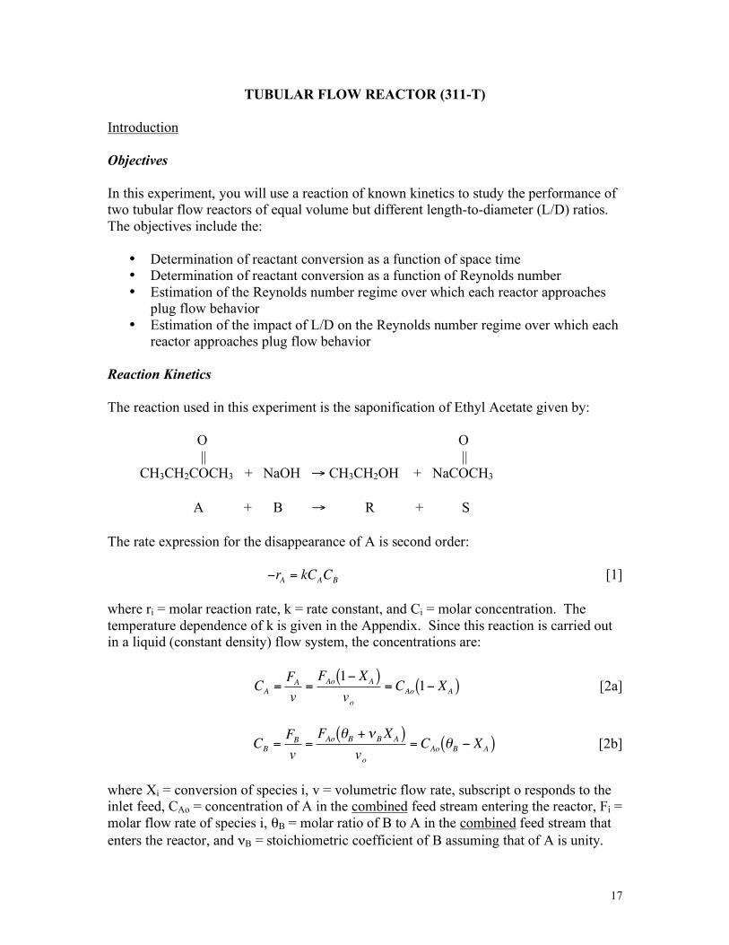
TUBULAR FLOW REACTOR (311-T) Introduction Objectives In this experiment, you will use a reaction of known kinetics to study the performance of two tubular flow reactors of equal volume but different length-to-diameter (L/D) ratios. The objectives include the:

• Determination of reactant conversion as a function of space time • Determination of reactant conversion as a function of Reynolds number • Estimation of the Reynolds number regime over which each reactor approaches

plug flow behavior • Estimation of the impact of L/D on the Reynolds number regime over which each

reactor approaches plug flow behavior Reaction Kinetics The reaction used in this experiment is the saponification of Ethyl Acetate given by:

O O || || CH3CH2COCH3 + NaOH → CH3CH2OH + NaCOCH3 A + B → R + S The rate expression for the disappearance of A is second order:

!

"rA

= kCACB

[1] where ri = molar reaction rate, k = rate constant, and Ci = molar concentration. The temperature dependence of k is given in the Appendix. Since this reaction is carried out in a liquid (constant density) flow system, the concentrations are:

!

CA

=FA

v=FAo1" X

A( )vo

= CAo1" X

A( ) [2a]

!

CB

=FB

v=FAo"B

+ #BXA( )

vo

= CAo"B$ X

A( ) [2b]

where Xi = conversion of species i, v = volumetric flow rate, subscript o responds to the inlet feed, CAo = concentration of A in the combined feed stream entering the reactor, Fi = molar flow rate of species i, θB = molar ratio of B to A in the combined feed stream that enters the reactor, and νB = stoichiometric coefficient of B assuming that of A is unity.

18

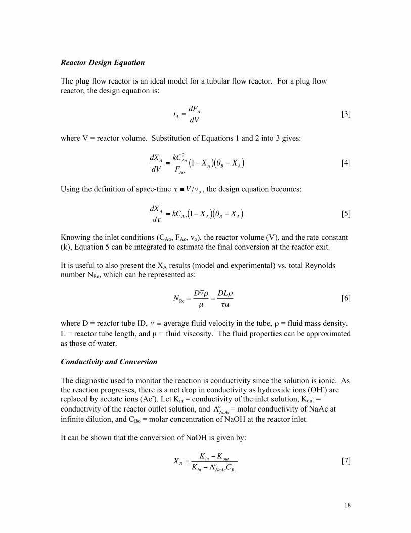
Reactor Design Equation The plug flow reactor is an ideal model for a tubular flow reactor. For a plug flow reactor, the design equation is:

!

rA

=dF

A

dV [3]

where V = reactor volume. Substitution of Equations 1 and 2 into 3 gives:

!

dXA

dV=kC

Ao

2

FAo

1" XA( ) #B " XA( ) [4]

Using the definition of space-time

!

" #V vo, the design equation becomes:

!

dXA

d"= kC

Ao1# X

A( ) $B # XA( ) [5]

Knowing the inlet conditions (CAo, FAo, vo), the reactor volume (V), and the rate constant (k), Equation 5 can be integrated to estimate the final conversion at the reactor exit. It is useful to also present the XA results (model and experimental) vs. total Reynolds number NRe, which can be represented as:

!

NRe

=Dv "

µ=

DL"

#µ [6]

where D = reactor tube ID,

!

v = average fluid velocity in the tube, ρ = fluid mass density, L = reactor tube length, and µ = fluid viscosity. The fluid properties can be approximated as those of water. Conductivity and Conversion The diagnostic used to monitor the reaction is conductivity since the solution is ionic. As the reaction progresses, there is a net drop in conductivity as hydroxide ions (OH-) are replaced by acetate ions (Ac-). Let Kin = conductivity of the inlet solution, Kout = conductivity of the reactor outlet solution, and

!

"NaAc

o = molar conductivity of NaAc at infinite dilution, and CBo = molar concentration of NaOH at the reactor inlet. It can be shown that the conversion of NaOH is given by:

!

XB

=K

in"K

out

Kin" #

NaAc

oCBo

[7]

19

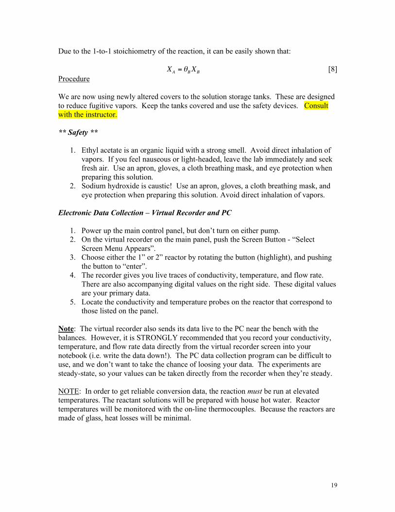
Due to the 1-to-1 stoichiometry of the reaction, it can be easily shown that:

!

XA

= "BXB

[8] Procedure We are now using newly altered covers to the solution storage tanks. These are designed to reduce fugitive vapors. Keep the tanks covered and use the safety devices. Consult with the instructor. ** Safety **

1. Ethyl acetate is an organic liquid with a strong smell. Avoid direct inhalation of vapors. If you feel nauseous or light-headed, leave the lab immediately and seek fresh air. Use an apron, gloves, a cloth breathing mask, and eye protection when preparing this solution.

2. Sodium hydroxide is caustic! Use an apron, gloves, a cloth breathing mask, and eye protection when preparing this solution. Avoid direct inhalation of vapors.

Electronic Data Collection – Virtual Recorder and PC

1. Power up the main control panel, but don’t turn on either pump. 2. On the virtual recorder on the main panel, push the Screen Button - “Select

Screen Menu Appears”. 3. Choose either the 1” or 2” reactor by rotating the button (highlight), and pushing

the button to “enter”. 4. The recorder gives you live traces of conductivity, temperature, and flow rate.

There are also accompanying digital values on the right side. These digital values are your primary data.

5. Locate the conductivity and temperature probes on the reactor that correspond to those listed on the panel.

Note: The virtual recorder also sends its data live to the PC near the bench with the balances. However, it is STRONGLY recommended that you record your conductivity, temperature, and flow rate data directly from the virtual recorder screen into your notebook (i.e. write the data down!). The PC data collection program can be difficult to use, and we don’t want to take the chance of loosing your data. The experiments are steady-state, so your values can be taken directly from the recorder when they’re steady. NOTE: In order to get reliable conversion data, the reaction must be run at elevated temperatures. The reactant solutions will be prepared with house hot water. Reactor temperatures will be monitored with the on-line thermocouples. Because the reactors are made of glass, heat losses will be minimal.

20

Dimensions of Solution Tanks Both solution tanks are 35 inches deep, with 22.5 inches ID. There are plastic meter sticks available. In addition, there are wooden dowels with depth marks. These are especially useful in making sure the tanks are filled with the proper amount of water. Preparation of Ethyl Acetate Solution

1. Estimate the height that will correspond to 50 gallons of solution. 2. Open the tank drain. Run hot water from the spigot through the tank until the

water is as hot as you feel it is going to get. 3. Turn on the exhaust system – consult with the instructor. 4. Close all drain valves under the tank, and fill with hot water to the required level.

Use a white plastic meter stick or wooden dip stick to judge depth. 5. Pull out the yellow hose, and screw on the metal cap (hand-tight). 6. Activate the pneumatic agitator. 7. Carefully, pour in ~ 2 liters of ethyl acetate (EtAc) – you might wish to use a

funnel. Try not to spill any. If you do, get the instructor. Screw on the metal cap (hand-tight).

8. Mix the contents of the tank for at least 10 minutes. Avoid inhalation of any vapors. If you smell organic vapors, get the instructor.

9. Estimate the EtAc solution concentration in the tank. It should be ~ 0.11 mole/liter. 10. Turn off the agitator for the ethyl acetate tank by closing the air valve on the motor.

Standardization of Ethyl Acetate Tank Solution

1. Close both yellow-handled valves feeding the reactor tubes. Leave open the valve leading to the glass drain pipe. Close the silver-handled valve on the NaOH line, but leave the corresponding valve on the EtAc line open a little.

2. Align the feed tank valves for flow to the EtAc pump. 3. Activate main power. Then turn on the EtAc pump. 4. Look for a small flow rate (< 1 gpm) directly to the drain. After flowing for about

10 seconds, use the black-handled sample valve to extract a sample (~ 50 ml) of the EtAc solution. Make sure you purge the sample line first.

5. Close the sample valve, and turn off the pump. 6. Using a pipet, extract about 20 ml of EtAc solution from your container. 7. Put a 10 ml sample of the EtAc solution into a 150 ml flask. 8. Add 20 ml the standardized NaOH solution (~ 0.1N NaOH) from the tank

prepared below into the flask. 9. Put a Teflon-coated stirring bar into the flask, and place the flask onto a magnetic

stirrer. Agitate the mixture for about 2 hours to ensure that the reaction has gone to completion (i.e. all EtAc has been consumed).

10. Place a few drops of phenolphthalein indicator into the flask. 11. Use a standardized HCl solution (0.1N HCl) available on the lab bench to titrate

the solution to its end point.

21

12. Since the amount of NaOH added is known, and this titration gives the amount of NaOH remaining, the amount of NaOH that reacted with the EtAc is known. From this, the EtAc concentration in the tank can be calculated.

13. Determine the concentration of EtAc in the tank, based on this titration procedure. Compare this value to your earlier estimate. If the values are very different, consult with the instructor. NOTE: Remember that this value is not CAo.

Preparation of Sodium Hydroxide Solution for Reaction 1) Estimate the height that will correspond to 50 gallons of solution. 2) Open the tank drain. Run hot water from the spigot through the tank until the water is

as hot as you feel it is going to get. 3) Close all valves exiting the feed tank, and fill with hot water to the required level. Use

a wooden dip stick or a white meter stick to judge depth. Withdraw the yellow hose, and screw on the metal cap (hand-tight).

4) From the available supply, prepare ~ 830 grams of dry NaOH into a convenient container.

5) Activate the pneumatic agitator, and make sure the exhaust fan is running. 6) Pour dry NaOH into the tank. Use a funnel if you wish. Try hard not to spill the

NaOH powder. If you do, dry-brush it into the garbage pail. Screw on the cap. 7) Stir the tank for at least 10 minutes. Avoid inhalation of any vapors. 8) Estimate the NaOH solution concentration based on how much you used. It should

correspond to ~ 0.11 mole/liter. 9) Turn off the agitator for the NaOH tank by closing the air valve on the motor. Standardization of Sodium Hydroxide Tank Solution 1. Close both yellow-handled valves feeding the reactor tubes. Leave open the valve

leading to the glass drain pipe. Close the silver-handled valve on the EtAc line, but leave the corresponding valve on the NaOH line open a little.

2. Align the feed tank valves for flow to the NaOH pump. 3. Activate main power. Then turn on the NaOH pump. 4. Look for a small flow rate (< 1 gpm) directly to the drain. After flowing for about 10

seconds, use the black-handled sample valve to extract a sample (~ 50 ml) of the NaOH solution. Make sure you purge the sample line first.

5. Close the sample valve, and turn off the pump. 6. With a pipet, withdraw about 20 ml of solution into a flask. 7. Place a 10 ml sample of NaOH from the feed tank into a flask. 8. Place a few drops of phenolphthalein indicator into the flask. Use a standardized HCl

solution (~ 0.1N HCl) from the lab bench to titrate the NaOH solution to its end point. 9. Determine the concentration of NaOH, and compare to your earlier estimate. If these

are vastly different, consult the instructor. Remember that this value is not CBo.

22

Reactor Runs and Data Collection NOTE: Keep the tanks covered, and the exhaust fan running. The pneumatic mixers should remain turned off.

1. Set the inlet valves to direct the combined feed to the particular reactor chosen in step 3 above on the virtual recorder.

2. Plan for 5-6 runs per reactor, starting with the highest flow rates that can be achieved down to low rates in roughly equal increments. Starting with the maximum equal flow rates will help purge any air from the reactor tubes.

3. For each run, activate the feed pumps, and set the two reactant solutions to the same flow rate as registered on the virtual recorder. Equal volumetric flow rates will make sure you have the same θB for all runs.

4. After each pair of flow rates are set, allow the system to come to steady state by observing the live signals from the relevant conductivity probes. You should wait at least time equivalent to 1-2 times τ for the particular flow rates. So, for example, if the τ = 0.5 minutes for the particular run, you should wait at least 30-60 seconds for probe stabilization. Record the conductivity and temperature data from the reactor, carefully note the units posted on the recorder, for each flow rate.

5. After steady state data are recorded for a given run, the flow rates should be changed. This judgment can be easily made be visually dividing the feed tanks into ~ six equal parts (by volume) and changing the feed rates at the end of each part. Avoid running the feed pumps dry.

6. When the 1-inch diameter reactor study is complete, repeat this procedure and study the 2-inch diameter reactor, or vice-versa. You might wish to plan the second reactor for another lab period using tanks of fresh solution.

Clean-Up

1. Upon completion of the experiments for a given lab period, drain the feed tanks of any remaining solution using the drain valves. Rinse both tanks out with water.

2. Flush out the reactor that you have just studied with plain water for at least 2 min. 3. Don’t forget to complete any solution standarizations. 4. Rinse out any glassware used on the bench. Turn off the magnetic stirrer. 5. Make sure all burets are isolated by closing all discharge valves. 6. Police the general area, making sure not to leave a mess. If spills have occurred,

consult the TA or the instructor. Data Analysis, Modeling, and Discussion

Reactor Analysis

1. For each reactor, plot the observed exit XA vs. space-time (τ). On the same graph, plot the predicted exit XA vs. τ based on integration of Equation 5. Make sure you use the average temperature for the reactor, based on the thermocouple data, to calculate the correct k value.

23

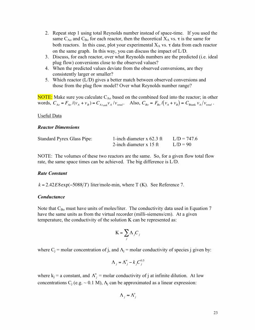
2. Repeat step 1 using total Reynolds number instead of space-time. If you used the same CAo and CBo for each reactor, then the theoretical XA vs. τ is the same for both reactors. In this case, plot your experimental XA vs. τ data from each reactor on the same graph. In this way, you can discuss the impact of L/D.

3. Discuss, for each reactor, over what Reynolds numbers are the predicted (i.e. ideal plug flow) conversions close to the observed values?

4. When the predicted values deviate from the observed conversions, are they consistently larger or smaller?

5. Which reactor (L/D) gives a better match between observed conversions and those from the plug flow model? Over what Reynolds number range?

NOTE: Make sure you calculate CAo based on the combined feed into the reactor; in other words,

!

CAo

= FAo/(v

A+ v

B) = C

A tankvA/v

total. Also,

!

CBo

= FBo/ v

A+ v

B( ) = CBtank

vAvtotal

. Useful Data Reactor Dimensions Standard Pyrex Glass Pipe: 1-inch diameter x 62.3 ft L/D = 747.6 2-inch diameter x 15 ft L/D = 90 NOTE: The volumes of these two reactors are the same. So, for a given flow total flow rate, the same space times can be achieved. The big difference is L/D. Rate Constant

!

k = 2.42E8exp("5088 T) liter/mole-min, where T (K). See Reference 7. Conductance Note that CBo must have units of moles/liter. The conductivity data used in Equation 7 have the same units as from the virtual recorder (milli-siemens/cm). At a given temperature, the conductivity of the solution Κ can be represented as:

!

" = # jC j

j

$

where Cj = molar concentration of j, and Λj = molar conductivity of species j given by:

!

" j = " j

#$ k jC j

0.5 where kj = a constant, and

!

" j

# = molar conductivity of j at infinite dilution. At low concentrations Cj (e.g. ~ 0.1 M), Λj can be approximated as a linear expression:

!

" j # " j

o

24

where

!

" j

o is a function of temperature. Therefore,

!

" = f C j ,T( ) . Based on data obtained from the literature and experimentally in this lab, the following are recommended: NaOH (up to 0.2 Molar)

!

" j

o= #0.0241T

2+ 5.0658T +111.13 (

!

" j

o in mS/cm/Molar, T in oC) NaAc (up to ~ 0.1 Molar)

!

" j

o=1.546T + 27.695 (

!

" j

o in mS/cm/Molar, T in oC) References

1. Kendall, H. B., Chem. Eng. Prog. Symp. Series, No. 70, Vol. 63, p.3–15 (1967). 2. Hovorka, R. B. and Kendall, H. B., Chem. Eng. Prog., 56, No. 8, p. 58-62 (1960). 3. Cleland, F. A. and Wilhelm, R. H., AICHE Journal 2, 489 (1956). 4. Fogler, H. S., “Elements of Chemical Reaction Engineering”, 4th Ed., Prentice

Hall, Englewood Cliffs, New Jersey (2006). 5. Bamford, C., C. Tipper. 1970. Comp. Chem. Kinetics v.10. Elsevier. N.Y. p.169. 6. Data from B. B. Conway, Electrochemical Dam (New York: Elsevier, 1952). 7. www.uni-

r.de/Fakultaeten/nat_Fak_IV/Organische_Chemie/Didaktik/Keusch/chembox_etac-e.htm

25

SEMI-BATCH REACTOR (311-T) Introduction Objectives In this experiment, you will use a reaction of known kinetics to study the performance of a semi-batch reactor. The objectives include: • Observation of solution conductivity and temperature, and evolved oxygen rate,

as functions of time for three different reactant feed rates • Comparison of these measured quantities to predicted values based on an ideal

semi-batch reactor model • Estimation of unmeasured reactant concentrations based on the ideal model

Reaction and Kinetics The reaction used in this experiment is inspired by Shams El Din and Mohammed (1998), who studied the kinetics of this reaction as a means to remove residual bleach from water purification equipment.

H2O2(aq) + NaOCl(aq) → H2O(l) + NaCl(aq) + O2(g)

A + B → R + S + T The letters representing the species are shown in corresponding order. The reported rate expression for the disappearance of A is second order:

!

"rA

= kCACB

= "rB

= rS

= rT [1]

where ri = reaction rate of species i, k = reaction rate constant, and Ci = molar concentration of i. Because the reaction evolves gaseous O2 rather rapidly, it is preferred to run it in a semi-batch reactor. To start, a batch vessel contains hydrogen peroxide (H2O2 – species A) in a water solution. The aqueous solution of sodium hypochlorite (NaOCl – species B) is fed slowly over time at a constant rate. As shown above, species S and T are NaCl and O2, respectively. Reactor Species Balances A semi-batch design equation applies for B:

!

FB

+ rBV =

dNB

dt [2]

where FB = molar flow rate inlet to the batch, V = batch liquid volume, and Ni = moles of i in the batch. A simple batch design equation applies for A:

26

!

rAV =

dNA

dt [3]

The inlet molar flow rate of B can be written in more convenient volumetric terms:

B

BBBB

W

fvF

!= [4]

where vB = volumetric feed rate of B, ρB = bleach mass density, fB = mass fraction of species B in the feed bleach solution, and WB = molecular weight of B. Since

!

Ni= C

iV ,

and that V = f(t) in the most general semi-batch case, Eq. 3 becomes:

!

rA"CA

V

dV

dt=dC

A

dt [5]

and Eq. 2 becomes:

!

FB

V+ r

B"CB

V

dV

dt=dC

B

dt [6]

The rate of change of the volume is accounted for with a transient mass balance:

( )dt

Vdv

BB

!! = [7]

where ρ = mass density of batch solution. It can be reasonably assumed

B!! " ; then,

Eq. 7 reduces to:

!

vB

=dV

dt [8]

The volumetric feed rate of B is set at a constant value by the user in the experiment. Equations 1, 4, 5, 6, and 8 form a system that is solved simultaneously. The system is integrated from t = 0 (when the reactant B solution flow begins) to whenever the peroxide feed is ended by the user. Evolution of O2 Assuming that the bleach solution mixes thoroughly into the peroxide solution, the reaction mixture will likely saturate with O2 very rapidly. We can assume that the O2 evolution rate is approximately the same as the reaction rate, and is given by:

!

FT" r

TV [9]

27

The Ideal Gas Law can be used to convert FT to a volumetric rate.

!

rTVRT

s

Ps

" vT

[10]

where Ts, Ps represent standard temperature and pressure conditions (298 K, 1 atm), respectively, and R = ideal gas constant (0.0821 liter-atm/mole-K). Equation 10 can be added to the set of equations to be solved. The volumetric rate of evolved O2 is one of two possible sources of data in this experiment. The rate rT is obtained from Eq. 1. Conductivity Change The conductivity of a solution is a weighted sum of the contributions of the ionic species, including NaOCl as the active ingredient, a small amount of NaOH to help prevent degradation of NaOCl to release Cl2, and residual NaCl from the bleach manufacturing process. We assume that CNaOCl in the SBR is very small, and insignificantly contributes to the solution conductivity. Subsequent SBR modeling supports this claim. The batch solution conductivity can be estimated as:

!

C = c i

i

" Ci# c

NaClC

NaCl+ c

NaOHC

NaOH (11)

where C = solution conductivity,

!

c i = effective molar conductivity of species i, Ci =

molar concentration of i. Accounting for the contribution of NaCl to the solution conductivity requires a non-reactive species balance due to the presence of NaCl in the bleach feed:

!

FS

V+ r

S"CS

V

dV

dt=dC

S

dt (12)

The inlet molar flow rate of S (i.e. NaCl) can be written in more convenient volumetric terms:

S

SBBS

W

fvF

!= (13)

where fS = mass fraction of NaCl in the feed bleach solution. Molar conductivity

!

c NaCl

data for NaCl aqueous solutions are available over the temperature range of interest to yield a relationship valid up to 0.85 molar concentration:

!

c NaCl

= 0.0117Tc

2+1.3737T

c+ 51.665 (

!

c NaCl

in mS/cm/molar, Tc in oC) (14) Accounting for the contribution of NaOH to the solution conductivity requires a non-reactive species balance. Representing NaOH as the inert I, the balance is:

28

!

FI

V"CI

V

dV

dt=dC

I

dt (15)

The inlet molar flow rate of I can be written in more convenient volumetric terms:

I

IBBI

W

fvF

!= (16)

where fI = mass fraction of NaOH in the feed bleach solution. Molar conductivity

!

"NaOH

o data for NaOH aqueous solutions are available over the temperature range of interest to yield a relationship valid up to 0.3 molar concentration:

!

"NaOH

o= #0.0241T

c

2+ 5.0658T

c+111.13 (

!

"NaOH

o in mS/cm/molar, Tc in oC) (17) Equations 1, 4, 5, 6, 8, and 10, together with Equations 11, 13, 14, 15, 16, and 17 form a complete model. Energy Balance The energy balance should reflect the configuration of the reactor vessel. In a typical experiment, the liquid is in contact with stainless steel walls and internal components (e.g. agitator, probes). An air-filled jacket surround the walls. Heat losses to this metal must be considered. A simple heat loss calibration can be performed wherein an electric immersion heater of known wattage is placed in the vessel filled with water covering the metal parts (see instructor if there is time). A simple heat balance of this calibration is:

!

dT

dt=

Qh

mwcpw + mmcpm (18a)

where Qh = electrical heating rate, mw and mm = masses of water and metal parts respectively, and cpw and cpm = mass-based specific heats of water and metal respectively. A successful linear regression of the measured temperature vs. time, according to the integrated form of Eq. 18a, yielded a heat loss calibration of mmcpm = 1284 cal/oC. Consult the instructor as to whether or not this step will be verified. It can be shown, consistent with Fogler and Gurmen (2006) that the reactor energy balance is:

!

dT

dt=

" Fjocp j

T f

T

# dT +V "rA( ) "$HrA( )j

% + PdV

dt

mmcpm +V cp jC j

j

%

&

'

( ( ( ( (

)

*

+ + + + +

(18b)

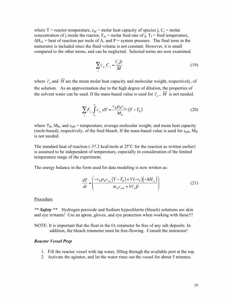
29

where T = reactor temperature, cpj = molar heat capacity of species j, Cj = molar concentration of j inside the reactor, Fjo = molar feed rate of j, Tf = feed temperature, ΔHrA = heat of reaction per mole of A, and P = system pressure. The final term in the numerator is included since the fluid volume is not constant. However, it is small compared to the other terms, and can be neglected. Selected terms are now examined.

!

cp jC j =

j

"c p#

M (19)

where

pc and M are the mean molar heat capacity and molecular weight, respectively, of

the solution. As an approximation due to the high degree of dilution, the properties of the solvent water can be used. If the mass-based value is used for

pc , M is not needed.

!

Fjocp j

T f

T

" dTj

# $vB%BcpBMB

T &TB( ) (20)

where TB, MB, and cpB = temperature, average molecular weight, and mean heat capacity (mole-based), respectively, of the feed bleach. If the mass-based value is used for cpB, MB is not needed. The standard heat of reaction (-37.2 kcal/mole at 25oC for the reaction as written earlier) is assumed to be independent of temperature, especially in consideration of the limited temperature range of the experiment. The energy balance in the form used for data modeling is now written as:

!

dT

dt="vB#BcpB

T "TB( ) + V "rA( ) "$HrA( )

mmcpm + Vc p#

%

&

' '

(

)

* *

(21)

Procedure ** Safety ** Hydrogen peroxide and Sodium hypochlorite (bleach) solutions are skin and eye irritants! Use an apron, gloves, and eye protection when working with these!!! NOTE: It is important that the float in the O2 rotameter be free of any salt deposits. In

addition, the bleach rotameter must be free-flowing. Consult the instructor! Reactor Vessel Prep

1. Fill the reactor vessel with tap water, filling through the available port at the top. 2. Activate the agitator, and let the water rinse out the vessel for about 5 minutes.

30

3. Fill the external bleach reservoirs with water, and circulate the water through the bleach system. Direct water to the reactor, making sure the bleach flowmeter operates freely.

4. Once all components have been rinsed, drain all water.

Activation of the Vessel Agitator

1. Insert the key card into the control box if not already present. 2. Turn on the unit by using the switch on the lower orange box accessible with your

right hand. If the display does not turn on, make sure the switch on the back of the upper box is on.

3. Hit the pad key under “Fermentation”; then hit the pad key under “Act”. 4. Hit the pad key for “Loop 1”; then hit 4, then finally hit the “act” key again. The

agitator should begin turning, and achieve a rate of 300 rpm. Verify this visually. 5. To temporarily turn off the agitator, hit the Stop key. Then, as prompted, hit the

Stop key again. Verify this visually. 6. To restart the agitator, hit the key pad for the “Main” menu. Then, repeat steps 3-4.

Reactor Runs and Data Collection 1. Make sure the vessel drain is closed. The, carefully add 3 liters of chilled hydrogen

peroxide solution to the vessel. Be careful loading the liquids!! Use goggles and gloves!! 2. Plug the fill hole with the black stopper – make sure it’s tight! 3. Make sure the external reservoir valve is closed. Then, carefully fill both reservoirs with

household bleach. Use a small ladder to enhance your reach if needed. Use care!! 4. Start the agitator. 5. Turn on the interfaces connecting the conductivity probe to the PC. 6. Activate the Logger Lite data collection program on the desktop. Upon opening, the PC

will be ready to collect and plot live conductivity data. Using the “Experiment” pull down menu, set for data collection rate for 1 point per second, and for “continuous” data.

7. Open bleach reservoir valve, and make sure valve directing bleach into reactor is closed! 8. Turn on the bleach pump, and circulate bleach back to the reservoir. 9. “Startup” involves the following simultaneous and coordinated actions:

a. Turn on the timer b. Click on the data collection program. c. Open the valve directing bleach into the reactor, and QUICKLY setting the

bleach flow rate to the desired value (≈ 3 gallons/hour). 10. When all are in position and everything is ready, proceed with the “Startup”. Remember,

this experiment is time-dependent! 11. Record the time, the digital temperature, and the corresponding O2 flow meter float level

(center of ball) – try to catch the near-initial maximum value. Record the rotameter and temperature readings every 10 seconds.

12. Continue data collection until bleach in the reservoir is exhausted. 13. When the run is complete, stop the PC data collection, and save these data. Do this by a

simple copy/paste of the data columns on the left of the screen into an Excel spreadsheet. 14. Close the two bleach valves.

31

15. Drain the reactor contents into a bucket, and dispose into the sink. Do not spill!! 16. Repeat the Reactor Vessel Prep (i.e. rinse out the reactor with water). 17. Drain the reactor contents into the bucket. 18. Repeat steps 1-15 on this section for ≈ 5 and 7 gallons/hour bleach rates. 19. Make sure you email your data files to your account, or download onto a flash drive.

Clean-Up

1. After the final run, carefully drain the reactor contents into the bucket, and dispose of into the sink.

2. Fill the external reservoir with water, and circulate water through the pump and into the vessel to wash out all bleach components.

3. Drain the reactor contents, and dispose. Then, fill the reactor with water, agitate for a five minutes, and then drain for a last time.

4. Power down all components, and clean up the general area. 5. Make sure the instructor is alerted to clean out the O2 rotameter, if needed.

Data, Analysis, and Discussion The model defined by Equations 1, 4, 5, 6, 8, 10-17, 21, 22 is solved with a numerical ordinary differential equation solver package. Be especially attentive to units! The rate constant used in Equation 1 is estimated from the data of Shams and Mohammed (1998).

!"

#$%

& '()

RTk

11800exp102

12 liter/mole-sec (22)

where R = 1.987 cal/mole-K, and T = absolute temperature (K). For each run, plot and discuss the predicted and observed batch solution conductivity, O2 evolution rate, and temperature, respectively. As a point of discussion, and lacking direct concentration measurements, the model profiles for CA and CB should be plotted also. Are the predicted concentrations of NaOCl in the batch sufficient small to warrant the assumption made earlier? Useful Data Household bleach: • Composition: 6.15 wt.% NaOCl, 0.36 wt.% NaOH, 2.9 wt.% NaCl, balance H2O • Specific gravity: 1.1 Hydrogen peroxide solution: 3 wt.% H2O2, balance water. Flow Meter Calibrations Oxygen ---- The evolved gas rate rO2 = rT (in standard liters/min), as read in the middle of the float, is given by:

!

rO2 = 0.059* reading

32

Bleach ---- Even though the new bleach rotameter is pre-calibrated for water, it has been calibrated for bleach, which is 10% more dense than water. The recommended calibration for bleach is: actual bleach rate (GPH) = 1.0679 * float reading – 0.5694 References Fogler and Gurmen, Elements of Chemical Reaction Eng., 4th ed., Prentice-Hall (2006). Haji, Shaker and Erkey, Can, Chemical Engineering Education 39(1), 56-61 (2005). Shams El Din, A. M. and Mohammed, R. A., “Kinetics of the reaction between hydrogen peroxide and hypochlorite,” Desalination, vol. 115, pp. 145-153 (1998). Clorox MSDS: http://www.thecloroxcompany.com/products/msds/ Powel web site: http://www.powellfab.com/technical_information/preview/general_info_about_sodium_hypo.asp

Landolt, H. and R. Bornstein, Zahlenwerte und Funktionen aus Naturwissenschaften und Technik., K. H. Hellwege (ed.), Volume 2, Part. Volume 6, Springer-Verlag, Berlin (1987) ---- obtained via Honeywell Sensing and Control, Freeport, IL.

33

Liquid Level Control #1 (B-7-T) Introduction Objectives In this experiment, you will evaluate the performance of a liquid-level control system. The objectives include:

• Determination of the transfer functions of several key components of the system • Operation and simulation of the system under feedback control

System and Theory Figure 1 is a sketch of the apparatus. A liquid stream enters the tank at a flow rate x(t) and leaves at a flow rate of u(t). The control elements include a liquid level transducer, liquid level computer controller-recorder (LCC), and an automatic control valve. The controller and automatic valve maintain the level in the tank, y(t), after a disturbance in the load variable, x(t). The level signal y(t) is produced by a transducer located at the bottom of the tank. It converts the pressure caused by the liquid height into a digital signal to the LCC. This signal is compared to a user-input set-point. The LCC calculates the error and transmits a digital signal to a digital-analog converter. The electric analog signal is converted to an air pressure (pneumatic) signal to the valve. The valve position allows for an increase or decrease in the effluent rate, u(t), and brings the level to its desired value.

Figure 1. Schematic Drawing of System

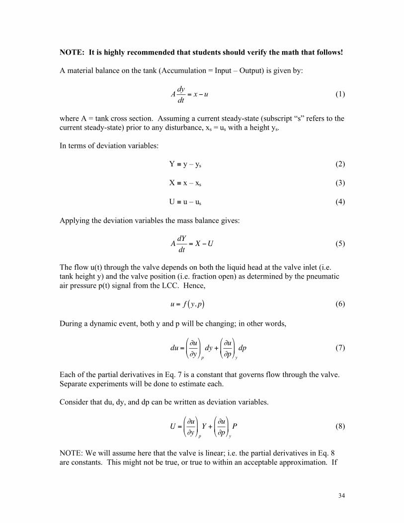
34

NOTE: It is highly recommended that students should verify the math that follows! A material balance on the tank (Accumulation = Input – Output) is given by:

uxdt

dyA != (1)

where A = tank cross section. Assuming a current steady-state (subscript “s” refers to the current steady-state) prior to any disturbance, xs = us with a height ys. In terms of deviation variables:

Y ≡ y – ys (2)

X ≡ x – xs (3)

U ≡ u – us (4) Applying the deviation variables the mass balance gives:

!

AdY

dt= X "U (5)

The flow u(t) through the valve depends on both the liquid head at the valve inlet (i.e. tank height y) and the valve position (i.e. fraction open) as determined by the pneumatic air pressure p(t) signal from the LCC. Hence,

!

u = f y, p( ) (6) During a dynamic event, both y and p will be changing; in other words,

!

du ="u

"y

#

$ %

&

' ( p

dy +"u

"p

#

$ %

&

' ( y

dp (7)

Each of the partial derivatives in Eq. 7 is a constant that governs flow through the valve. Separate experiments will be done to estimate each. Consider that du, dy, and dp can be written as deviation variables.

!

U ="u

"y

#

$ %

&

' ( p

Y +"u

"p

#

$ %

&

' ( y

P (8)

NOTE: We will assume here that the valve is linear; i.e. the partial derivatives in Eq. 8 are constants. This might not be true, or true to within an acceptable approximation. If

35

the subsequent modeling of our experimental data is poor, this valve assumption might be reconsidered. Now, for a fixed pneumatic pressure to the valve (i.e. dp = 0), and assuming a linear valve, Eq. 8 becomes:

!

U = c1Y (9)

where

!

c1

= "u "y . Substituting Eq. 9 into Eq. 5, and applying the LaPlace transform, we get:

!

Y s( ) =X s( )As+ c

1

=K1

" p +1X s( ) =GdX s( ) (10)

where K1 ≡ 1/c1, τp ≡ A/c1, and the tank transfer function is given by:

!

Gd "K1

# ps+1 (10a)

For a step change equal to “a” in inlet flow rate (gpm), X(s) = a/s. Substituted into Eq. 8,

!

Y (s) =K1

" ps+1

a

s=Gd

a

s (11)

Eq. 11 can be written in terms of partial fractions :

!

Y s( ) = K1a1

s"

# p# ps+1( )

$

% & &

'

( ) ) (12)

Apply the inverse LaPlace transform to get the open-loop system response:

!

Y t( ) = K1a 1" e

" t # p( ) (13) A curve-fit of experimental Y(t) vs. t data according to Eq. 13 should yield τp, K1, and c1. System and Theory – Valve Transfer Function In order to estimate the second partial derivative in Eq. 7, we will make no change in the inlet flow rate (i.e. X = 0). Rather, we will change the pneumatic pressure to the valve. However, recognize that the changing tank height will also change the flow through the valve. In other words, we must use Eq. 8 to model this phase:

!

U = c1Y + c

2P (14)

36

where

!

c2

= "u "p . For a pneumatic valve, the transient relationship between valve opening and applied pressure can be as complex as second order (Stephanopoulos, 1984). This suggests that c2 might not be a constant. For the moment, consider that it is. Substituting Eq. 14 into Eq. 5, together with X = 0, we get:

!

AdY

dt= "c

1Y " c

2P (15)

Applying the LaPlace transform to Eq. 15, we get:

!

Y s( ) ="c

2

As+ c1

P s( ) =K2

# ps+1P s( ) =GvP s( ) (16)

where K2 ≡ -c2/c1, and the valve transfer function is given by:

!

Gv "K2

# ps+1 (16a)

For a step change equal to “b” in pressure (psi) to the outlet valve, P(s) = b/s. Substituted into Eq. 16,

!

Y (s) =K2

" ps+1

b

s=Gv

b

s (17)

Eq. 17 can be written in terms of partial fractions :

!

Y s( ) = K2b1

s"

# p# ps+1

$

% &

'

( ) (18)

Apply the inverse LaPlace transform to get the open-loop system response:

!

Y t( ) = K2b 1" e

" t # p( ) (19) A curve-fit of experimental Y(t) vs. t data according to Eq. 19 should yield τp, K2, and c2. System and Theory – Controller Interface to Valve A careful review of the Procedure, the equipment, and the LCC user interface will reveal that the pneumatic pressure to the outlet valve is manipulated only by use of the outlet valve slider; i.e., setting a “% Closed” value will set a pressure. When the system is under feedback control, the controller will set the pressure to the valve through the setting of a valve slider. This relationship must be determined experimentally. In theory, we can assume the following for the outlet valve:

37

p = K3 %c + c4 (20)

where c3 and c4 are constants, %c = % closed on the outlet valve slider, and p = pneumatic pressure to the valve. Using deviation variables, Eq. 20 becomes:

P = K3 %C (21) Application of LaPlace transforms to Eq. 21 yields:

P(s) = K3 %C(s) (22) Also note that a linear relationship is assumed to exist between the height in the tank y(t) and the electrical signal b(t) sent from the transducer. Unlike the valve slider, the signal b(t) is effectively “invisible” to us. In addition, we can assume an essentially instantaneous transfer of y(t) to the error determination block of the LCC (i.e. the comparison between the actual height and the setpoint height). Going directly to the transfer function formulation, we can say:

B(s) = Gm Y(s) (23) where we can take the measurement transfer function Gm = 1.

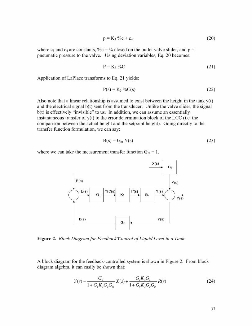
Figure 2. Block Diagram for Feedback Control of Liquid Level in a Tank A block diagram for the feedback-controlled system is shown in Figure 2. From block diagram algebra, it can easily be shown that:

!

Y (s) =G

d

1+GvK3G

cG

m

X(s) +G

vK3G

c

1+GvK3G

cG

m

R(s) (24)

38

Changes in the input flow rate to the tank are given by X(s), while changes in the tank height set-point are given by R(s). Tank, valve, and height transducer transfer functions – Gd, Gv, and K3 respectively – are determined experimentally. Typically, Gm = 1. The controller transfer function Gc depends on your choice of controller: proportional (P), proportional-integral (PI), or proportional-integral-derivative (PID). Three controller modes will be compared in this study. The controller output is the %closed setting on the outlet valve slider [%C(t); In LaPlace terms, %C(s)]. The error is the difference between the setpoint and the measured tank level [E(t) = R(t)-Y(t) since Gm = 1; in LaPlace term, E(s) = R(s) – Y(s)]. 1. Proportional Control For proportional control, the controller output is directly proportional to the error.

%C(t) = Kc E(t) (25) Applying LaPlace transforms, Eq. 25 becomes:

%C(s) = Kc E(s) (27) where Gc = Kc = proportional controller Gain. 2. Proportional-Integral Control For proportional-integral control, the controller output also depends on the accumulated error. In this way, offsets can generally be eliminated.

!

%C t( ) = KcE t( ) +

Kc

"i

E t( )dt0

t

# (28)

Applying LaPlace transforms, Eq. 28 becomes :

!

%C s( ) = KcE s( ) +

Kc

"isE s( ) = K

c1+

1

"is

#

$ %

&

' ( E s( ) (29)

where

!

Gc

= Kc1+1 "

is( )( ) = PI controller gain.

3. Proportional-Integral-Derivative Control For proportional-integral-derivative control, the controller output also depends on the rate of change of the error. In this way, instabilities can be avoided.

!

%C t( ) = KcE t( ) +

Kc

"i

E t( )dt0

t

# + Kc"d

dE t( )dt

(30)

39

Applying LaPlace transforms, Eq. 30 becomes :

!

%C s( ) = KcE s( ) +

Kc

"isE s( ) + K

c"dsE s( ) = K

c1+

1

"is

+ "ds

#

$ %

&

' ( E s( ) (31)

where

!

Gc

= Kc1+1 "

is( ) + "

ds( ) = PID controller gain.

OUR STRATEGY : As seen from Eq. 24, there are two classes of experiments that can be performed : disturbance in input flow rate X(s), or a change in set point R(s). With three types of controllers, this suggests six possible experiments – far too many. In order to get the flavor of feedback control problems, two problems will be required: I) Change in set point under P control, and II) Disturbance under PI control. If time allows, you are free to choose a problem. 4. Example of Feedback Control (P controller) For example, using proportional control only (Gc = Kc) with a change in set point problem [X(s) = 0], Equation 24 reduces to:

!

Y (s) =G

vK3G

c

1+GvK3G

cG

m

R(s) (32)

Substituting for Gv (from Eq. 16a) and Gm = 1, Eq. 32 becomes:

!

Y (s) =

K2K3Kc

" ps+1

1+K2KcK3

" ps+1

R(s) =K2KcK3

1+ " ps+ K2KcK3

R s( ) (33)

For a step change r (inches) in set point, R(s) = r/s. Also, let K0 ≡ 1 + K3K2Kc. Hence, Equation 33 becomes:

!

Y (s) =r Ko "1( )s # ps+ Ko( )

=r Ko "1( ) # p

s s+Ko

# p

$

% & &

'

( ) )

=r Ko "1( )Ko

Ko # p

s s+Ko

# p

$

% & &

'

( ) )

(34)

Applying the inverse LaPlace transform, Eq. 34 becomes:

!

Y t( ) =r Ko "1( )Ko

1" e"Kot # p( ) (35)

40

Equation 35 predicts the controlled first order response of the deviation height in the tank with proportional control for a step change in setpoint equal to “r”. 5. Example of Feedback Control (PI controller) For example, using proportional-integral control only [

!

Gc

= Kc1+1 "

is( )( )] with a feed

disturbance problem [R(s) = 0], Equation 24 reduces to:

!

Y (s) =G

d

1+GvK

c1+

1

"is

#

$ %

&

' ( K3

Gm

X(s) (36)

Substituting for Gd (from Eq. 10a), Gv (from Eq. 16a), and Gm = 1, Eq. 36 becomes:

!

Y (s) =

K1

" ps+1

1+K2

" ps+1

#

$ % %

&

' ( ( 1+

1

" is

#

$ %

&

' ( KcK3

X(s) (37)

For a step change a (gpm) in inlet flow rate, X(s) = a/s. Hence, Equation 37 becomes:

!

Y (s) =aK

1" p

s2

+Ko

" ps+

Ko #1

" i" p

(38)

where Ko ≡ 1 + K3K2Kc. Eq. 38 must be converted in order to utilize a convenient inverse LaPlace Transform:

!

LaPlace"1 #

s+$( )2

+# 2

%

& ' '

(

) * *

= e$t sin #t( ) (39)

Letting

!

" =Ko

2# pand

!

" =Ko #1

$ i$ p#Ko

2

4$ p2

%

& '

(

) *

0.5

, Eq. 38 becomes:

!

Y (s) =aK

1

" p#

$

% & &

'

( ) )

#

s+*( )2

+# 2[ ] (40)

Applying the inverse LaPlace transform:

41

!

Y (s) =aK1

" p#

$

% & &

'

( ) ) e

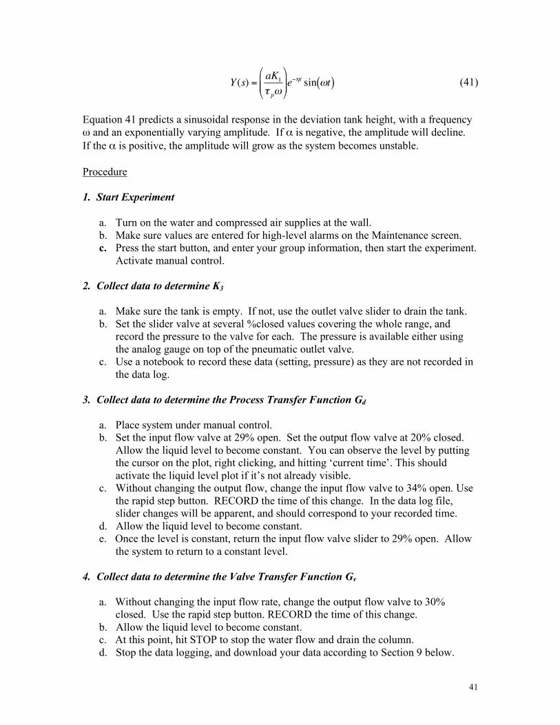
*+tsin #t( ) (41)

Equation 41 predicts a sinusoidal response in the deviation tank height, with a frequency ω and an exponentially varying amplitude. If α is negative, the amplitude will decline. If the α is positive, the amplitude will grow as the system becomes unstable. Procedure 1. Start Experiment

a. Turn on the water and compressed air supplies at the wall. b. Make sure values are entered for high-level alarms on the Maintenance screen. c. Press the start button, and enter your group information, then start the experiment.

Activate manual control.

2. Collect data to determine K3 a. Make sure the tank is empty. If not, use the outlet valve slider to drain the tank. b. Set the slider valve at several %closed values covering the whole range, and

record the pressure to the valve for each. The pressure is available either using the analog gauge on top of the pneumatic outlet valve.

c. Use a notebook to record these data (setting, pressure) as they are not recorded in the data log.

3. Collect data to determine the Process Transfer Function Gd

a. Place system under manual control. b. Set the input flow valve at 29% open. Set the output flow valve at 20% closed.

Allow the liquid level to become constant. You can observe the level by putting the cursor on the plot, right clicking, and hitting ‘current time’. This should activate the liquid level plot if it’s not already visible.

c. Without changing the output flow, change the input flow valve to 34% open. Use the rapid step button. RECORD the time of this change. In the data log file, slider changes will be apparent, and should correspond to your recorded time.

d. Allow the liquid level to become constant. e. Once the level is constant, return the input flow valve slider to 29% open. Allow

the system to return to a constant level. 4. Collect data to determine the Valve Transfer Function Gv

a. Without changing the input flow rate, change the output flow valve to 30% closed. Use the rapid step button. RECORD the time of this change.

b. Allow the liquid level to become constant. c. At this point, hit STOP to stop the water flow and drain the column. d. Stop the data logging, and download your data according to Section 9 below.

42

5. Place the System under Automatic control (Proportional Control)

a. Click on PID on the screen to open the user interface for feedback control. a. Click on OUT to enable manipulation of the outlet valve for tank control. b. Click on LEVEL to enable the system for liquid level control. c. Set level control set point at 30 inches, and input valve slider to 15% open. d. Click on AUTO to activate the feedback control loop. e. Set Kc = value1 (proportional gain), τi = 0 (integral time), τd = 0 (derivative time).

The Kc value (%C / inch) within the range of 10-50 is recommended. f. Wait till the tank level is constant. g. Change the set point to 40 inches. Note the time. h. Wait until a new steady liquid level is achieved. i. Decrease the set point to 30 inches. Note the time. j. Wait until a new steady liquid level is achieved.

6. Place the System under Automatic control (Proportional-Integral Control)

a. Set level control set point at 30 inches, and input valve slider to 15% open. b. Set Kc = value1 (same as above), τi = value2, τd = 0. A τi value (sec) in the range 5-

10 is recommended. c. Wait till the tank level is constant. d. Make a step increase in the input valve slider to 30% open. Note the time. e. Wait until a new steady state is achieved. f. Make a step decrease in the input slider back to 15% open. Note the time. g. Wait until a new steady state is achieved.

7. Retrieving Data from the Computer and Ending the Experiment

a. Click “STOP” at the right end of the screen. b. Click “COPY” to change the file name same as student’s names or to modify the

file name as desired. c. Click “STOP LOGGING”. d. Click “OK” to confirm. e. Click “CREATE REPORT” to create report file (wait around five seconds). f. Click “OPEN REPORT” to see the data recorded. g. Attach your USB Flash drive. h. At the tool bar, click “FILE” then click “SAVE AS” to save the file in your USB

Flash Drive. i. Hit STOP. j. Turn off the main water supply and the compressed air supply at the wall.

Data Analysis and Discussion Note: Be careful to use correct and consistent units during all the steps that follow!

43

1. Estimation of K3 a. Retrieve the pneumatic pressure p vs. outlet valve slider %c (closed) data. b. Fit these data to a linear form according to Eq. 20. c. Estimate K3 from the slope.

2. Estimation of the Process Transfer Function Gd

a. Retrieve the height y(t) vs. time t data for the constant outlet valve pressure open-loop experiment.

b. Convert the y(t) data to deviation format Y(t). c. Convert the step change in inlet valve slider to a step change in actual flow rate

(i.e. the value a). d. Fit the experimental Y(t) vs. t data according to Eq. 13. e. Estimate τp, K1, and c1.

3. Estimation of the Outlet Valve transfer function Gv

a. Retrieve the height y(t) vs. time t data for the open-loop experiment where you applied a step change to the outlet valve slider %closed.

b. Convert the y(t) data to deviation format Y(t). c. Using Eq. 21 and your value of K3, calculate the step change in valve pressure

(i.e. the value b). d. Fit the experimental Y(t) vs. t data according to Eq. 19. e. Estimate τp, K2, and c2.

4. Modeling of the System Response under Proportional Control

a. Retrieve the height y(t) vs. time t data for the closed-loop (Proportional Gain only) experiment where you applied a step change to the setpoint.

b. Using your values or expressions for K3, Gv, Gm, and Gc , together with Eq. 35, predict the closed loop response to the step increase disturbance in inlet flow rate. Be sure to calculate y(t) --- the absolute tank height. Then, predict the system response to the step decrease disturbance in the inlet flow rate.

c. On a single plot, compare the experimental y(t) to the predicted y(t). d. Comment on how well your model performs. What are some possible sources of

any deviations? 5. Modeling of the System Response under Proportional-Integral Control

a) Retrieve the height y(t) vs. time t data for the closed-loop (Proportional Gain and Integral Rate only) experiment where you applied a step change disturbance to the inlet valve slider %open.

b) Using your values or expressions for Gd, Gv, Gm, and Gc to predict the coefficients in Eq. 41.

44

c) Predict the closed loop response to the step increase disturbance in inlet flow rate. Be sure to calculate y(t) --- the absolute tank height. Then, predict the system response to the step decrease disturbance in the inlet flow rate.

d) On a single plot, compare the experimental y(t) to the predicted y(t). e. Comment on how well your model performs. What are some possible sources of

any deviations? 6. Items to Consider in the Conclusion Compare the predicted system behaviors with the experimental behaviors. Consider and discuss sources of error in both the experiment and the model. Is the model for the control valve appropriate? What about the controller settings? References 1. Harriot, P., “Process Control”, McGraw-Hill Book Co., New York, N.Y. (1964). 2. Perlmutter, D.D., “Introduction to Process Control,” John Wiley & Sons, Inc.,

New York, N. Y. (1966). 3. Coughanowr, D.R., and Koppel, L.B., “Process Systems Analysis and Control”,

McGraw-Hill Book Co., New York, New York (1966). 4. Weber, Thomas W., “An Introduction to Process Dynamics and Control”, John

Wiley and Sons, Inc., New York, New York (1973). 5. Stephanopoulos, George, “Chemical Process Control – An Introduction to Theory

and Practice”, P T R Prentice Hall, Englewood Cliffs, New Jersey 07632 (1984). 6. Bequette, B., “Process Control: Modeling, Design and Simulation,” Prentice Hall,

Englewood Cliffs, New Jersey (2003).

45

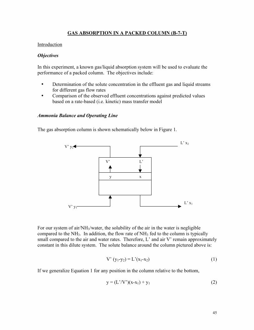
GAS ABSORPTION IN A PACKED COLUMN (B-7-T)

Introduction

Objectives In this experiment, a known gas/liquid absorption system will be used to evaluate the performance of a packed column. The objectives include: • Determination of the solute concentration in the effluent gas and liquid streams

for different gas flow rates • Comparison of the observed effluent concentrations against predicted values

based on a rate-based (i.e. kinetic) mass transfer model Ammonia Balance and Operating Line The gas absorption column is shown schematically below in Figure 1.

For our system of air/NH3/water, the solubility of the air in the water is negligible compared to the NH3. In addition, the flow rate of NH3 fed to the column is typically small compared to the air and water rates. Therefore, L’ and air V’ remain approximately constant in this dilute system. The solute balance around the column pictured above is:

V’ (y1-y2) = L’(x1-x2) (1) If we generalize Equation 1 for any position in the column relative to the bottom,

y = (L’/V’)(x-x1) + y1 (2)

V’ y2 L’ x2

L’ x1 V’ y1

V’ L’

y x

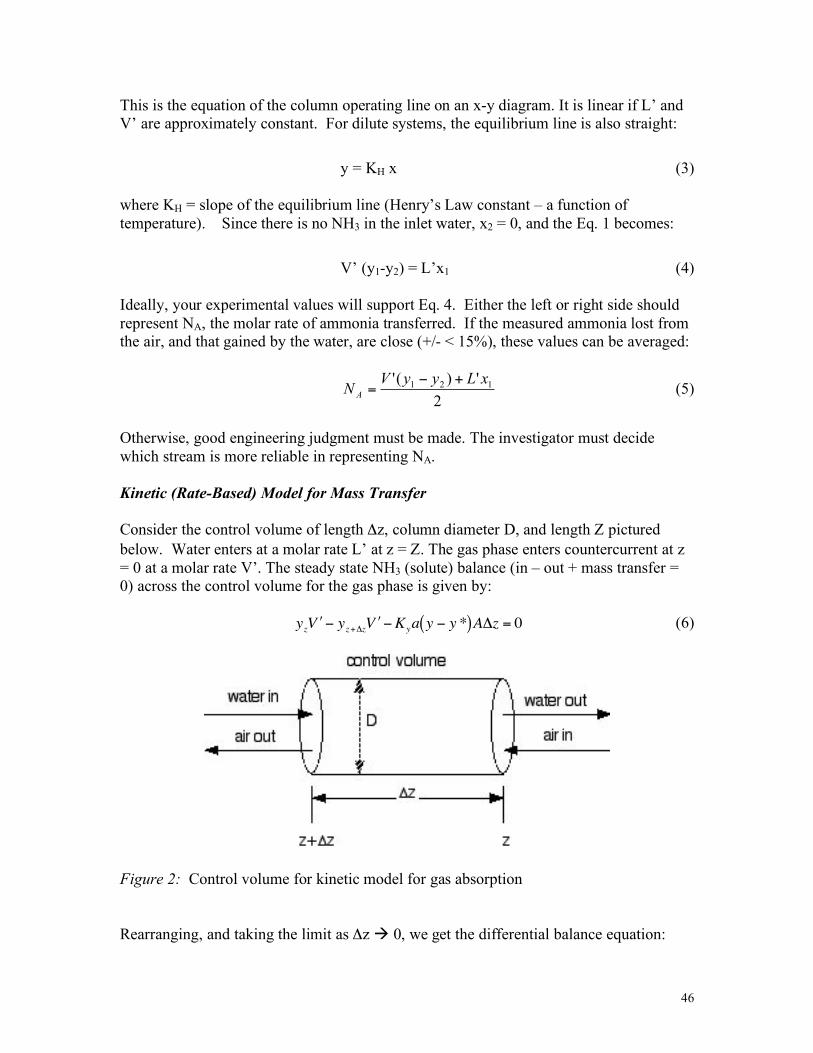
46

This is the equation of the column operating line on an x-y diagram. It is linear if L’ and V’ are approximately constant. For dilute systems, the equilibrium line is also straight:

y = KH x (3) where KH = slope of the equilibrium line (Henry’s Law constant – a function of temperature). Since there is no NH3 in the inlet water, x2 = 0, and the Eq. 1 becomes:

V’ (y1-y2) = L’x1 (4) Ideally, your experimental values will support Eq. 4. Either the left or right side should represent NA, the molar rate of ammonia transferred. If the measured ammonia lost from the air, and that gained by the water, are close (+/- < 15%), these values can be averaged:

2

')(' 121 xLyyVNA

+!= (5)

Otherwise, good engineering judgment must be made. The investigator must decide which stream is more reliable in representing NA. Kinetic (Rate-Based) Model for Mass Transfer Consider the control volume of length Δz, column diameter D, and length Z pictured below. Water enters at a molar rate L’ at z = Z. The gas phase enters countercurrent at z = 0 at a molar rate V’. The steady state NH3 (solute) balance (in – out + mass transfer = 0) across the control volume for the gas phase is given by:

!

yz" V # yz+$z

" V #Kya y # y *( )A$z = 0 (6)

Figure 2: Control volume for kinetic model for gas absorption Rearranging, and taking the limit as Δz 0, we get the differential balance equation:

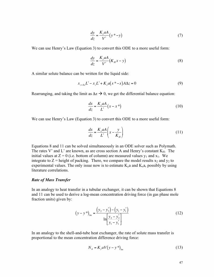
47

!

dy

dz=

KyaA

" V y *#y( ) (7)

We can use Henry’s Law (Equation 3) to convert this ODE to a more useful form:

!

dy

dz=

KyaA

" V K H x # y( ) (8)

A similar solute balance can be written for the liquid side:

!

xz+"z

# L $ xz# L + K

xa x *$x( )A"z = 0 (9)

Rearranging, and taking the limit as Δz 0, we get the differential balance equation:

!

dx

dz=

KxaA

" L x # x *( ) (10)

We can use Henry’s Law (Equation 3) to convert this ODE to a more useful form:

!

dx

dz=

KxaA

" L x #

y

K H

$

% &

'

( ) (11)

Equations 8 and 11 can be solved simultaneously in an ODE solver such as Polymath. The rates V’ and L’ are known, as are cross section A and Henry’s constant KH. The initial values at Z = 0 (i.e. bottom of column) are measured values y1 and x1. We integrate to Z = height of packing. There, we compare the model results x2 and y2 to experimental values. The only issue now is to estimate Kya and Kxa, possibly by using literature correlations. Rate of Mass Transfer In an analogy to heat transfer in a tubular exchanger, it can be shown that Equations 8 and 11 can be used to derive a log-mean concentration driving force (in gas phase mole fraction units) given by:

!

y " y *( )lm

=y2" y

2

*( ) " y1" y

1

*( )

lny2" y

2

*

y1" y

1

*

#

$ %

&

' (

(12)

In an analogy to the shell-and-tube heat exchanger, the rate of solute mass transfer is proportional to the mean concentration difference driving force:

!

NA = KyaV y " y *( )lm

(13)

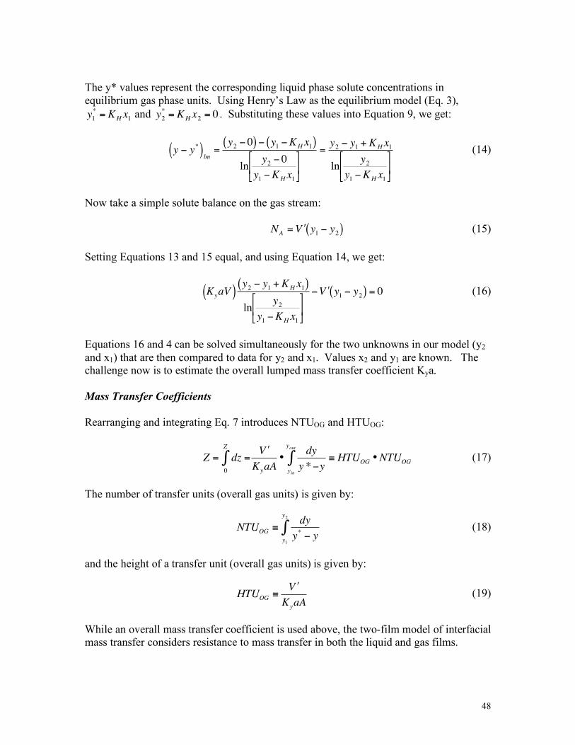
48

The y* values represent the corresponding liquid phase solute concentrations in equilibrium gas phase units. Using Henry’s Law as the equilibrium model (Eq. 3),

!

y1

*= KH x1 and

!

y2

*= KH x2 = 0 . Substituting these values into Equation 9, we get:

!

y " y*( )lm

=y2" 0( ) " y

1"KH x1( )

lny2" 0

y1"KH x1

#

$ %

&

' (

=y2" y

1+ KH x1

lny2

y1"KH x1

#

$ %

&

' (

(14)

Now take a simple solute balance on the gas stream:

!

NA = " V y1# y

2( ) (15) Setting Equations 13 and 15 equal, and using Equation 14, we get:

!

KyaV( )y2" y

1+ K H x

1( )

lny2

y1"K H x

1

#

$ %

&

' (

" ) V y1" y

2( ) = 0 (16)

Equations 16 and 4 can be solved simultaneously for the two unknowns in our model (y2 and x1) that are then compared to data for y2 and x1. Values x2 and y1 are known. The challenge now is to estimate the overall lumped mass transfer coefficient Kya. Mass Transfer Coefficients Rearranging and integrating Eq. 7 introduces NTUOG and HTUOG:

!

Z = dz =0

Z

"# V

KyaA•

dy

y *$yyin

yout

" % HTUOG • NTUOG (17)

The number of transfer units (overall gas units) is given by:

!

NTUOG "dy

y* # y

y1

y2

$ (18)

and the height of a transfer unit (overall gas units) is given by:

!

HTUOG "# V

KyaA (19)

While an overall mass transfer coefficient is used above, the two-film model of interfacial mass transfer considers resistance to mass transfer in both the liquid and gas films.

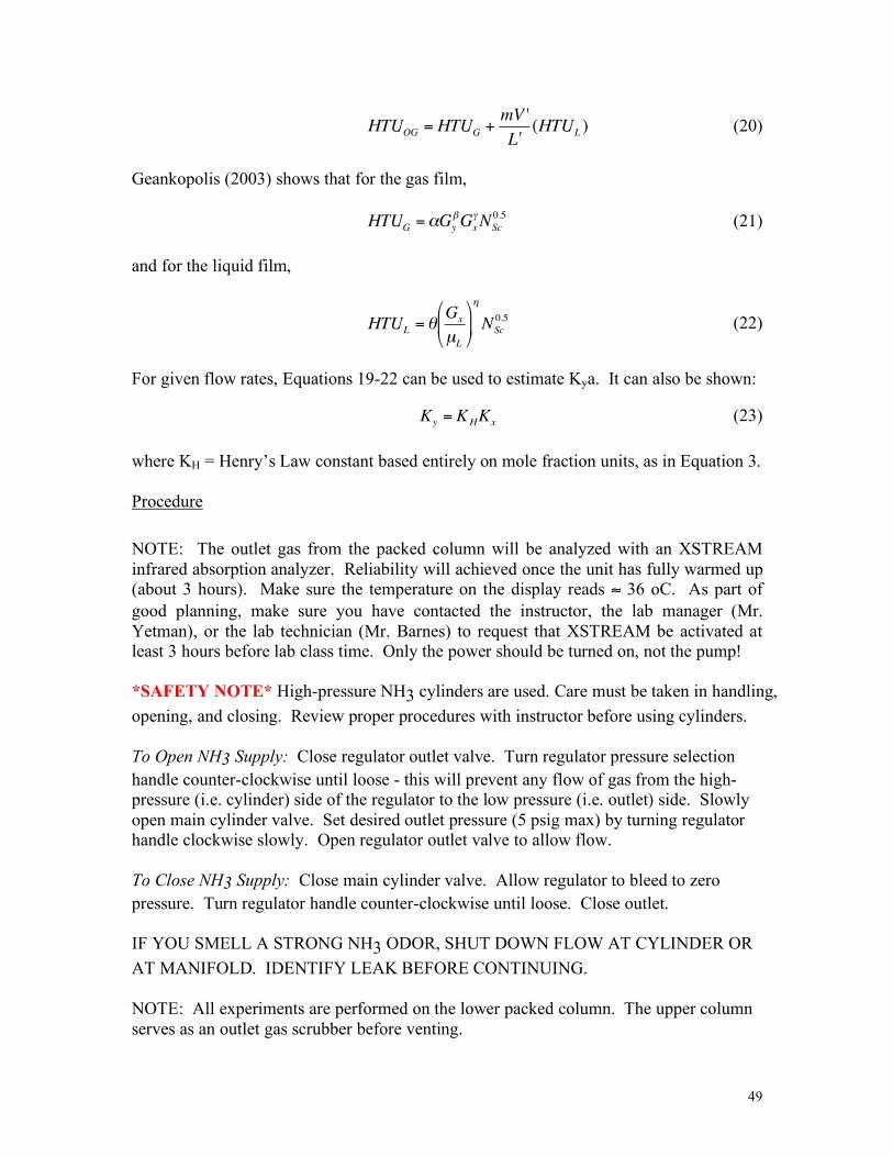
49

!

HTUOG

= HTUG

+mV '

" L (HTU

L) (20)

Geankopolis (2003) shows that for the gas film,

!

HTUG ="Gy

#Gx

$NSc

0.5 (21) and for the liquid film,

!

HTUL

= "G

x

µL

#

$ %

&

' (

)

NSc

0.5 (22)

For given flow rates, Equations 19-22 can be used to estimate Kya. It can also be shown:

!

Ky = KHKx (23)

where KH = Henry’s Law constant based entirely on mole fraction units, as in Equation 3. Procedure NOTE: The outlet gas from the packed column will be analyzed with an XSTREAM infrared absorption analyzer. Reliability will achieved once the unit has fully warmed up (about 3 hours). Make sure the temperature on the display reads ≈ 36 oC. As part of good planning, make sure you have contacted the instructor, the lab manager (Mr. Yetman), or the lab technician (Mr. Barnes) to request that XSTREAM be activated at least 3 hours before lab class time. Only the power should be turned on, not the pump! *SAFETY NOTE* High-pressure NH3 cylinders are used. Care must be taken in handling, opening, and closing. Review proper procedures with instructor before using cylinders. To Open NH3 Supply: Close regulator outlet valve. Turn regulator pressure selection handle counter-clockwise until loose - this will prevent any flow of gas from the high-pressure (i.e. cylinder) side of the regulator to the low pressure (i.e. outlet) side. Slowly open main cylinder valve. Set desired outlet pressure (5 psig max) by turning regulator handle clockwise slowly. Open regulator outlet valve to allow flow.

To Close NH3 Supply: Close main cylinder valve. Allow regulator to bleed to zero pressure. Turn regulator handle counter-clockwise until loose. Close outlet. IF YOU SMELL A STRONG NH3 ODOR, SHUT DOWN FLOW AT CYLINDER OR AT MANIFOLD. IDENTIFY LEAK BEFORE CONTINUING. NOTE: All experiments are performed on the lower packed column. The upper column serves as an outlet gas scrubber before venting.

50

NOTE: A water leg is used to seal the air flow into both packed columns. Identify them, and make sure they are full during all operations. Check “Zero” on the XSTREAM Analyzer NOTE: Do NOT perform this step unless asked to by the instructor. The analyzer is pre-

calibrated. This step is only needed for occasional verification.

1. The POWER and AC switches should already be on, and the analyzer warmed up for at least 3 hours. The SAMPLE pump should NOT be on.

2. Open the N2 zero gas cylinder. To open or close the N2 cylinder, follow the same

procedure as for the NH3 pressure regulator. Do NOT set the outlet pressure from N2 regulator above 10 psig. Consult the instructor if you are not sure.

3. Set the MODE selector switch on the black panel to ZERO. Flow zero gas (pure

N2). Set the SAMPLE rotameter to ~ 5.

4. Let the meter stabilize; it should read ~ 0 ppm. If not, consult the instructor. Once steady, turn off the N2 zero gas at the cylinder and regulator.

Ammonia Absorption Note: For all runs, set a water flow rates on both rotameters to 10. Monitor the rotameter

settings carefully, especially the rotameter for water to the lower column. Take note and record the column temperature using the round analog gauges available.

1. Set the NH3 rotameter to 100% (full capacity). Monitor and maintain for all runs. 2. For the fixed lower column water rate, begin with the air rate at 60% capacity on

its rotameter. Make sure you are not flooding either column or blowing their water seals as you CAREFULLY and slowly raise the air rate to 60%. If you cannot achieve 60% without blowing either column water seal, lower the air rate until you do.

a. Determine the steady state NH3 concentrations in the outlet gas stream

using the XSTREAM. Try to estimate the steady-state value even though the sensitivity and low concentrations cause reading fluctuations.

b. Draw a sample of outlet liquor, and determine the steady state NH3

concentration by titration with standard acid.

3. Lower the air rate to 50%, and repeat the steady-state measurements. Repeat this process for three more lower air rates at equal increments.

51

Ammonia Determination - Exit Gas Stream (only) A new infrared absorption analyzer (X-STREAM) will be used to determine the NH3 concentration in the outlet gaseous stream. This analyzer is shared with the neighboring Wetted Wall Column Absorption Experiment. Before directing gas samples to the analyzer, make sure the 3-way valves to the left of the base of the packed column (on right side of analyzer box) are set to accept gas samples from the Packed Column. Note that the upper limit of detection of the X-STREAM is ~ 30,000 ppm. Values much higher than this are not reliable. If you consistently obtain high values, see the instructor.

1. Make sure the valves as open for exit gas samples. 2. To sample gas from the tower, set MODE switch on the analyzer panel to

SAMPLE 2 (column outlet). Do not leave switch on AUTO.

3. Fully open BYPASS rotameter valves; turn on the SAMPLING PUMP.

4. Set SAMPLE rotameter to ~ 5. Carefully throttle back on the BYPASS flow if needed; otherwise, BYPASS rotameters should be fully open.

5. When finished, turn off the PUMP; return MODE switch to ZERO; flow ZERO

gas to flush the analyzer. When the meter reads ~ 0 ppm, turn off the ZERO gas at the cylinder and regulator. Turn off the POWER switch, and close the door.

Ammonia Determination - Exit Liquid Stream

1. Make sure sufficient time has elapsed from the time the air rate was set, and the liquid sample is drawn. Estimate this by using an estimate of the volume of the water seal leg under the lower column to the sample tube, and the water flow rate.

2. Draw a known volume sample (~ 10-20 ml) of the exit liquid below the column.

Use a container that is much larger than the sample volume (e.g. 100 ml flask for a 10 ml sample).

3. Add a few drops of indicator. Methyl red indicator is suggested since the

equivalence point should be slightly acidic due to the NH4Cl resulting from titration of dissolved NH3 with HCl (ph ~ 5, yellow red). NOTE: Keep adding the acid till the color change occurs. The volume required might be much larger than the sample volume.

4. At the same time you draw a liquid sample, activate the digital meter for the

dissolved NH3 probe. Check with the instructor first to see if probe is working – NOT available this semester.

52

5. Record the pH on the meter. Is this value consistent with the pH that you calculate based on the titration?

Ammonia Determination – Feed Gas Stream (only) NOTE: Use the calibrated rotameter flow rates to determine the NH3 concentration in the

feed stream. Do NOT use the XSTREAM for this purpose. Data Analysis, Modeling, and Discussion

1. Compute the NH3 mass balance for each run by tabulating both sides of Eq. 4. For a given run, if the two sides differ by less than ~ 20%, proceed with the analysis below. If not, consult with the instructor.

2. For each run, use Eqs. 19-22 to calculate Kya. Then, use Equations 4 and 16 to

estimate outlet concentrations x1 and y2. For the runs where the water rate was held constant, present the experimental and estimated concentrations as functions of the air rate.

3. Comment on how well you are able to simulate the exit concentrations.

Nomenclature a = surface area per unit volume of packing, ft2/ft3 or m2/m3 A = cross sectional area of packed column, ft2 or m2 Gy = superficial molar gas velocity, lbmoles/hr.ft2 or kg.moles/s.m2 Gx = superficial molar liquid velocity, lbmoles/hr.ft2 or kg.moles/s.m2 HTUG = individual height of transfer unit based upon gas phase, ft or m HTUL = individual height of transfer unit based upon liquid phase, ft or m HTUOG = height of a transfer unit, overall based on the gas phase, ft or m KH = Henry’s Law constant KYa = overall mass transfer coefficient based on gas phase, lb moles/ h – ft3 –mf or kg moles/h – m3 – mf L’ = molar liquid flow rate, lbmoles/hr or kg.moles/s m = slope of equilibrium line consistent mole fraction NH3 gas phase / mole fraction NH3 liquid phase; m = KH (Henry’s Law constant for this problem). NA = molar transfer rate of NH3, lbmoles/hr or kg.moles/s NOG = NTUOG = number of transfer units, overall based on gas phase NSc = Schmidt number used in correlations for HTUG and HTUL (Geankoplis, 2003). V = volume of packing in the column, ft3 or m3 V’ = molar vapor flow rate, lbmoles/hr or kg.moles/s x = concentration of NH3 in liquid phase, mole fraction y = concentration of NH3 in gas phase, mole fraction y* = concentration of NH3 in air at equilibrium with corresponding liquid of

concentration x, mole fraction z = length along the packing, ft or m

53

Z = total packing height, ft or m

!

",#,$,%,& = parameters in correlations for HTUG and HTUL (Geankoplis, 2003). µL = liquid viscosity used in correlations for HTUL (Geankoplis, 2003). Data KH = Henry’s Law constant or slope of the equilibrium curve = 0.85 mole fraction/mole fraction at 60 oF. If the column temperature is not 60 oF, consult the instructor. Data to estimate KH at other temperatures will be made available.

For Equations 21 for the gas film, HTUG = αGY

β GXγ NSc

0.5 where the units are: HTUG (m), GY (kg total gas/s – m2), GX (kg total liquid/s – m2). No data for ½ inch Raschig rings are given. As an approximation, use the following values for 3/8 inch Raschig rings to be used as an approximation: α = 0.620, β = 0.45, γ = - 0.47. The gas phase Schmidt Number NSc = µ/ρD, where µ = gas viscosity (kg/m-s), ρ = gas density (kg/m3), and D = diffusivity of ammonia in the gas phase (m2/s). For Equation 22 for the liquid film, HTUL = θ (GX/µL)η NSc

0.5 The gas phase Schmidt Number NSc = µ/ρD, where the units are: HTUL (m), θ = 7.18 x 10-4, η = 0.35, µL= liquid viscosity (kg/m-s), ρ = liquid density (kg/m3), D = Diffusivity of ammonia in the liquid phase (m2/s). References

1. Foust, A.S. et al, "Principles of Unit Operations," 1st Ed., John Wiley & Sons, Inc., New York, N.Y. (1980).

2. Dwyer, O.E. and Dodge, B.F., Ind. Eng. Chem. 33, No.4 p 484 (1941).

3. Sherwood, T.K.E., and Pigford, R.L., "Absorption and Extraction," 2nd Ed.,

McGraw-Hil1 Book Co., New York, N.Y. (1952).

4. Treybal, R.E., "Mass Transfer Operations," 2nd Ed., McGraw-Hill, New York (1968).

5. Geankopolis, C. J., “Transport Process and Separation Process Principles

(Includes Unit Operation)”, Fourth Edition, Prentice Hall, Upper Saddle River, NJ (2003).

6. McCabe, W. L., Smith, J. C., and Harriot, P., “Unit Operation of Chemical

Engineering”, Fifth Edition, McGraw-Hall, Inc., New York, NY, (1993).

54

Liquid Level Control #2 (B-7-T) NOTE: In this experiment, tests are to be conducted on the liquid level portion of the

system typically used in ChE 396 for the Transient Heat Transfer experiment. No heat transfer will be used here for ChE 496.

Introduction Objectives In this experiment, you will evaluate the performance of a liquid-level control system. The objectives include:

• Determination of the transfer functions of several key components of the system • Operation and simulation of the system under feedback control

System and Theory – Mass Balance Figure 1 is a sketch of the apparatus. A liquid stream enters the tank at a flow rate x(t) and leaves at a flow rate of u(t). The control elements include a liquid level sensor, level computer controller (LCC), and an pneumatic control valve. The controller and valve maintain the level in the tank, y(t), after a disturbance in the load variable, x(t). The level signal y(t) is produced by a sensor immersed into the tank. It converts the height of the liquid into an electrical signal to the LCC. This signal is compared to a user-input set-point. The LCC calculates the error and transmits a digital signal to a digital-analog converter. The electric analog signal is converted to an air pressure (pneumatic) signal to the valve. The valve position allows for an increase or decrease in the effluent rate, u(t). NOTE: It is highly recommended that students should verify the math that follows! A material balance on the tank (Accumulation = Input – Output) is given by:

uxdt

dyA != (1)

where A = tank cross section. Assuming a current steady-state (subscript “s” refers to the current steady-state) prior to any disturbance, xs = us with a height ys. In terms of deviation variables:

Y ≡ y – ys (2)

X ≡ x – xs (3)

U ≡ u – us (4)

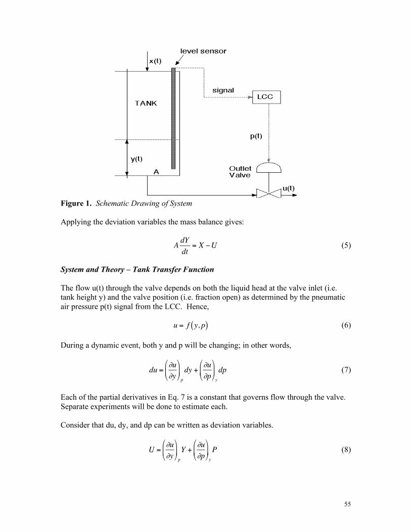
55

Figure 1. Schematic Drawing of System Applying the deviation variables the mass balance gives:

!

AdY

dt= X "U (5)

System and Theory – Tank Transfer Function The flow u(t) through the valve depends on both the liquid head at the valve inlet (i.e. tank height y) and the valve position (i.e. fraction open) as determined by the pneumatic air pressure p(t) signal from the LCC. Hence,

!

u = f y, p( ) (6) During a dynamic event, both y and p will be changing; in other words,

!

du ="u

"y

#

$ %

&

' ( p

dy +"u

"p

#

$ %

&

' ( y

dp (7)

Each of the partial derivatives in Eq. 7 is a constant that governs flow through the valve. Separate experiments will be done to estimate each. Consider that du, dy, and dp can be written as deviation variables.

!

U ="u

"y

#

$ %

&

' ( p

Y +"u

"p

#

$ %

&

' ( y

P (8)

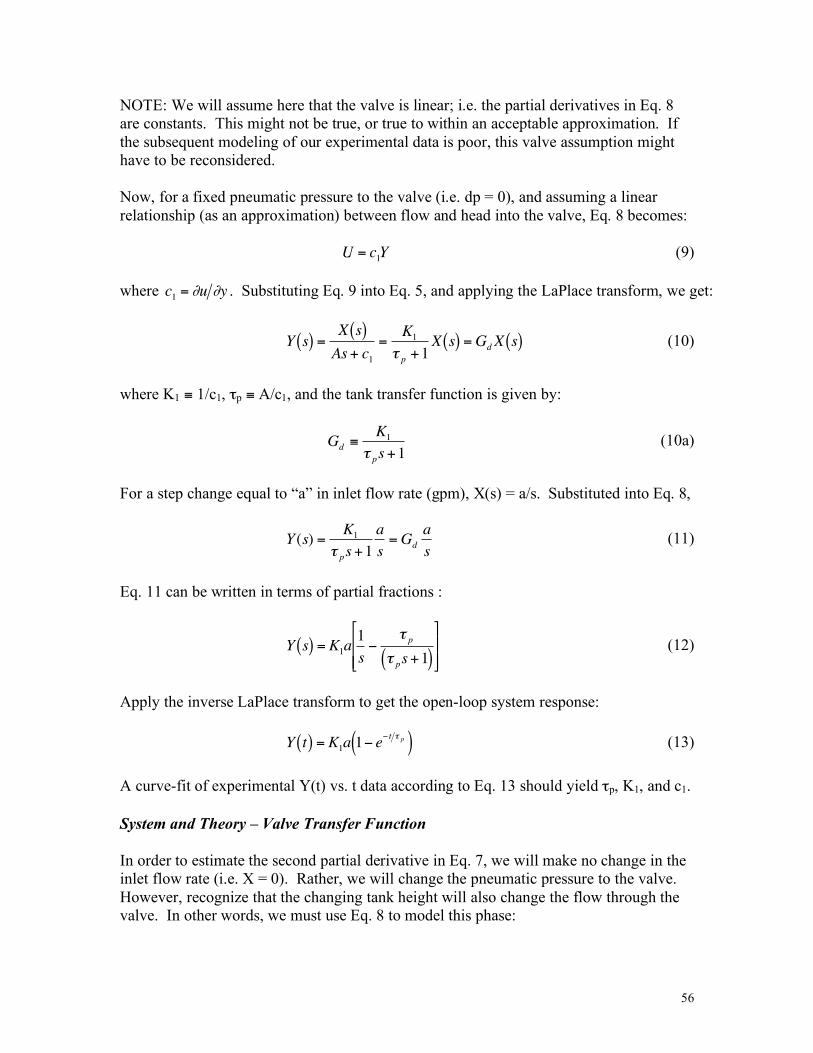
56

NOTE: We will assume here that the valve is linear; i.e. the partial derivatives in Eq. 8 are constants. This might not be true, or true to within an acceptable approximation. If the subsequent modeling of our experimental data is poor, this valve assumption might have to be reconsidered. Now, for a fixed pneumatic pressure to the valve (i.e. dp = 0), and assuming a linear relationship (as an approximation) between flow and head into the valve, Eq. 8 becomes:

!

U = c1Y (9)

where

!

c1

= "u "y . Substituting Eq. 9 into Eq. 5, and applying the LaPlace transform, we get:

!

Y s( ) =X s( )As+ c

1

=K1

" p +1X s( ) =GdX s( ) (10)

where K1 ≡ 1/c1, τp ≡ A/c1, and the tank transfer function is given by:

!

Gd "K1

# ps+1 (10a)

For a step change equal to “a” in inlet flow rate (gpm), X(s) = a/s. Substituted into Eq. 8,

!

Y (s) =K1

" ps+1

a

s=Gd

a

s (11)

Eq. 11 can be written in terms of partial fractions :

!

Y s( ) = K1a1

s"

# p# ps+1( )

$

% & &

'

( ) ) (12)

Apply the inverse LaPlace transform to get the open-loop system response:

!

Y t( ) = K1a 1" e

" t # p( ) (13) A curve-fit of experimental Y(t) vs. t data according to Eq. 13 should yield τp, K1, and c1. System and Theory – Valve Transfer Function In order to estimate the second partial derivative in Eq. 7, we will make no change in the inlet flow rate (i.e. X = 0). Rather, we will change the pneumatic pressure to the valve. However, recognize that the changing tank height will also change the flow through the valve. In other words, we must use Eq. 8 to model this phase:

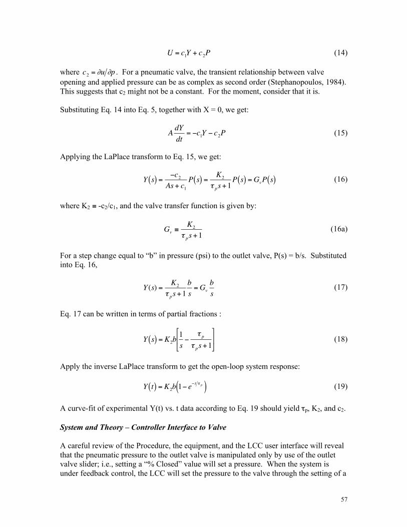
57

!

U = c1Y + c

2P (14)

where

!

c2

= "u "p . For a pneumatic valve, the transient relationship between valve opening and applied pressure can be as complex as second order (Stephanopoulos, 1984). This suggests that c2 might not be a constant. For the moment, consider that it is. Substituting Eq. 14 into Eq. 5, together with X = 0, we get:

!

AdY

dt= "c

1Y " c

2P (15)

Applying the LaPlace transform to Eq. 15, we get:

!

Y s( ) ="c

2

As+ c1

P s( ) =K2

# ps+1P s( ) =GvP s( ) (16)

where K2 ≡ -c2/c1, and the valve transfer function is given by:

!

Gv "K2

# ps+1 (16a)

For a step change equal to “b” in pressure (psi) to the outlet valve, P(s) = b/s. Substituted into Eq. 16,

!

Y (s) =K2

" ps+1

b

s=Gv

b

s (17)

Eq. 17 can be written in terms of partial fractions :

!

Y s( ) = K2b1

s"

# p# ps+1

$

% &

'

( ) (18)

Apply the inverse LaPlace transform to get the open-loop system response:

!

Y t( ) = K2b 1" e

" t # p( ) (19) A curve-fit of experimental Y(t) vs. t data according to Eq. 19 should yield τp, K2, and c2. System and Theory – Controller Interface to Valve A careful review of the Procedure, the equipment, and the LCC user interface will reveal that the pneumatic pressure to the outlet valve is manipulated only by use of the outlet valve slider; i.e., setting a “% Closed” value will set a pressure. When the system is under feedback control, the LCC will set the pressure to the valve through the setting of a

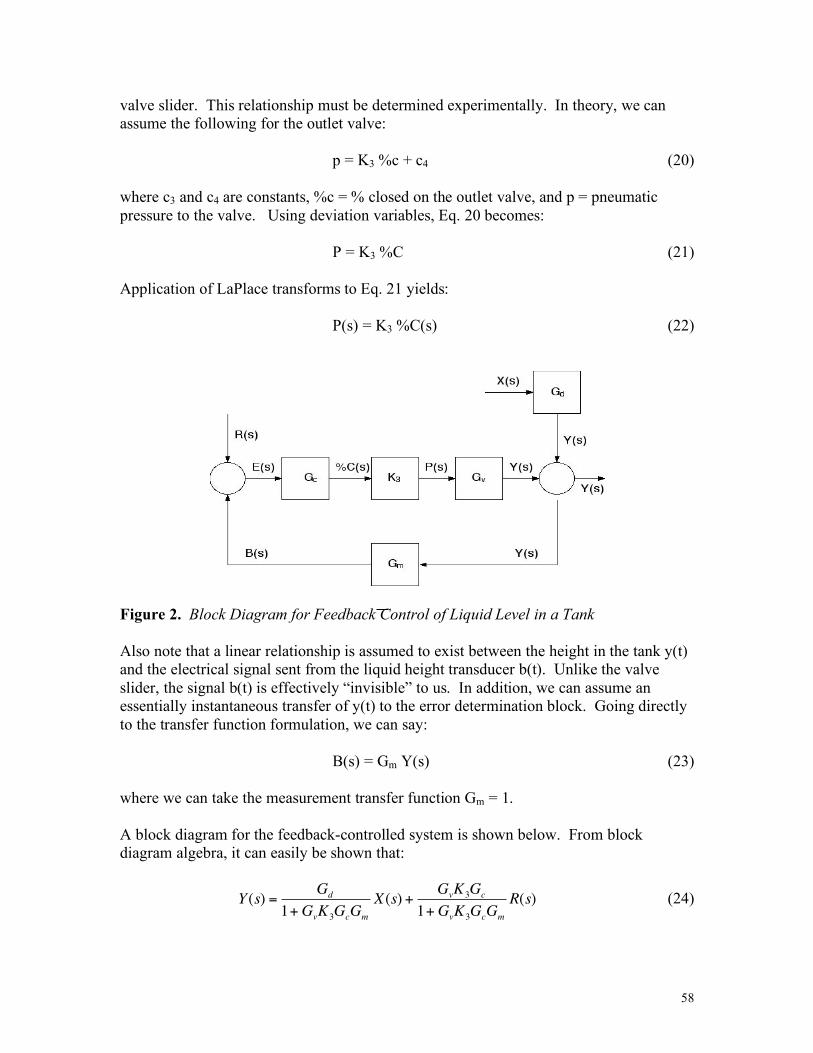
58

valve slider. This relationship must be determined experimentally. In theory, we can assume the following for the outlet valve:

p = K3 %c + c4 (20) where c3 and c4 are constants, %c = % closed on the outlet valve, and p = pneumatic pressure to the valve. Using deviation variables, Eq. 20 becomes:

P = K3 %C (21) Application of LaPlace transforms to Eq. 21 yields:

P(s) = K3 %C(s) (22)

Figure 2. Block Diagram for Feedback Control of Liquid Level in a Tank Also note that a linear relationship is assumed to exist between the height in the tank y(t) and the electrical signal sent from the liquid height transducer b(t). Unlike the valve slider, the signal b(t) is effectively “invisible” to us. In addition, we can assume an essentially instantaneous transfer of y(t) to the error determination block. Going directly to the transfer function formulation, we can say:

B(s) = Gm Y(s) (23) where we can take the measurement transfer function Gm = 1. A block diagram for the feedback-controlled system is shown below. From block diagram algebra, it can easily be shown that:

!

Y (s) =G

d

1+GvK3G

cG

m

X(s) +G

vK3G

c

1+GvK3G

cG

m

R(s) (24)

59

Changes in the input flow rate to the tank are given by X(s), while changes in the tank height set-point are given by R(s). Valve and height transducer transfer functions, Gv and K3 respectively, are either determined experimentally. Typically, Gm = 1. The controller transfer function Gc depends on your choice of controller: proportional (P), proportional-integral (PI), or proportional-integral-derivative (PID). Three controller modes will be compared in this study. The controller output is the %closed setting on the outlet valve slider [%C(t); In LaPlace terms, %C(s)]. The error is the difference between the setpoint and the measured tank level [E(t) = R(t)-Y(t) since Gm = 1; in LaPlace term, E(s) = R(s) – Y(s)]. 1. Proportional Control For proportional control, the controller output is directly proportional to the error.

%C(t) = Kc E(t) (25) Applying LaPlace transforms, Eq. 25 becomes:

%C(s) = Kc E(s) (27) where Gc = Kc = proportional controller Gain. 2. Proportional-Integral Control For proportional-integral control, the controller output also depends on the accumulated error. In this way, offsets can generally be eliminated.

!

%C t( ) = KcE t( ) +

Kc

"i

E t( )dt0

t

# (28)

Applying LaPlace transforms, Eq. 23 becomes :

!

%C s( ) = KcE s( ) +

Kc

"isE s( ) = K

c1+

1

"is

#

$ %

&

' ( E s( ) (29)

where

!

Gc

= Kc1+1 "

is( )( ) = PI controller gain.

3. Proportional-Integral-Derivative Control For proportional-integral-derivative control, the controller output also depends on the rate of change of the error. In this way, instabilities can be avoided.

!

%C t( ) = KcE t( ) +

Kc

"i

E t( )dt0

t

# + Kc"d

dE t( )dt

(30)

60

Applying LaPlace transforms, Eq. 30 becomes :

!

%C s( ) = KcE s( ) +

Kc

"isE s( ) + K

c"dsE s( ) = K

c1+

1

"is

+ "ds

#

$ %

&

' ( E s( ) (31)

where

!

Gc

= Kc1+1 "

is( ) + "

ds( ) = PID controller gain.

OUR STRATEGY : As seen from Eq. 24, there are two classes of experiments that can be performed : disturbance in input flow rate X(s), or a change in set point R(s). With three types of controllers, this suggests six possible experiments – far too many. In order to get the flavor of feedback control problems, two problems will be required: I) Change in set point under P control, and II) Disturbance under PI control. If time allows, you are free to choose a problem. 4. Example of Feedback Control (P controller) For example, using proportional control only (Gc = Kc) with a change in set point problem [X(s) = 0], Equation 24 reduces to:

!

Y (s) =G

vK3G

c

1+GvK3G

cG

m

R(s) (32)

Substituting for Gv (from Eq. 16a) and Gm = 1, Eq. 32 becomes:

!

Y (s) =

K2K3Kc

" ps+1

1+K2KcK3

" ps+1

R(s) =K2KcK3

1+ " ps+ K2KcK3

R s( ) (33)

For a step change r (inches) in set point, R(s) = r/s. Also, let K0 ≡ 1 + K3K2Kc. Hence, Equation 33 becomes:

!

Y (s) =r Ko "1( )s # ps+ Ko( )

=r Ko "1( ) # p

s s+Ko

# p

$

% & &

'

( ) )

=r Ko "1( )Ko

Ko # p

s s+Ko

# p

$

% & &

'

( ) )

(34)

Applying the inverse LaPlace transform, Eq. 34 becomes:

!

Y t( ) =r Ko "1( )Ko

1" e"Kot # p( ) (35)

61

Equation 35 predicts the controlled first order response of the deviation height in the tank with proportional control for a step change in setpoint equal to “r”. 5. Example of Feedback Control (PI controller) For example, using proportional-integral control only [

!

Gc

= Kc1+1 "

is( )( )] with a feed

disturbance problem [R(s) =0], Equation 24 reduces to:

!

Y (s) =G

d

1+GvK

c1+

1

"is

#

$ %

&

' ( K3

Gm

X(s) (36)

Substituting for Gd (from Eq. 10a), Gv (from Eq. 16a), and Gm = 1, Eq. 36 becomes:

!

Y (s) =

K1

" ps+1

1+K2

" ps+1

#

$ % %

&

' ( ( 1+

1

" is

#

$ %

&

' ( KcK3

X(s) (37)

For a step change a (gpm) in inlet flow rate, X(s) = a/s. Hence, Equation 37 becomes:

!

Y (s) =aK

1" p

s2

+Ko

" ps+

Ko #1

" i" p

(38)

where Ko ≡ 1 + K3K2Kc. Eq. 38 must be converted in order to utilize a convenient inverse LaPlace Transform:

!

LaPlace"1 #

s+$( )2

+# 2

%

& ' '

(

) * *

= e$t sin #t( ) (39)

Letting

!

" =Ko

2# pand

!

" =Ko #1

$ i$ p#Ko

2

4$ p2

%

& '

(

) *

0.5

, Eq. 38 becomes:

!

Y (s) =aK

1

" p#

$

% & &

'

( ) )

#

s+*( )2

+# 2[ ] (40)

Applying the inverse LaPlace transform:

62

!

Y (s) =aK1

" p#

$

% & &

'

( ) ) e

*+tsin #t( ) (41)

Equation 41 predicts a sinusoidal response in the deviation tank height, with a frequency ω and an exponentially varying amplitude. If α is negative, the amplitude will decline. If the α is positive, the amplitude will grow as the system becomes unstable. Procedure Take careful note of the user interface screens. You are NOT using heat transfer in this experiment - only liquid level control. You will need a flash drive and a notebook. 1. Start Experiment

a. Turn on the water and compressed air supplies at the wall. b. Make sure the regulated air supply pressure reads 20 psig. Do NOT turn on the

steam! Do NOT turn on the agitator.

2. Collect data to determine K3 a. On the HOME screen, click on Batch Valve Control. b. Keep the Inlet Valve slider at 0% Open; i.e., no inlet flow. c. Set the slider for the Drain Valve to several (at least five) ‘%closed’ values

covering the whole range (0-100%), and record the pressure to the outlet valve for each. The analog pressure gauge is located on the top of the pneumatic drain (outlet) valve. Let the pressure gauge stabilize after each change in slider. Note: This pressure is NOT recorded by the Data Logger, so you’ll have to record these data in a notebook.

d. When complete, set the Outlet valve slider to 0% closed. e. Select HOME to return to the main screen. f. Activate the Data Logging. Enter the required information. A blinking green

light indicates that data logging is active.

3. Collect data to determine the Process Transfer Function Gd

a. Activate the Batch Valve Control. Shrink and move this window, then activate the PID Tuning screen again so you can monitor the liquid level. Make sure the time scale is visible.

b. Open the manual ball valve under the tank. c. Using the sliders, set the input flow (CW) valve at 50% open, and the output

(Drain) flow valve at 50% closed. d. Open the water supply (oval handle) and the tank feed valves on the front panel. e. Visually, and on the screen, observe the liquid level. Do NOT overflow the tank! f. Let the liquid level become constant. Make minor adjustments in the output valve

slider in order to maintain a constant level for at least 5-10 minutes. The tank should be no more than ½ full.

63

g. Without changing the output flow, increase input flow valve to 65% open. Record the time on the bottom of the moving liquid level plot when you do this.

h. Allow the system to reach a constant level. Do NOT overflow the tank. If overflow is imminent, turn off the water supply valve, and start over.

i. Once the level is constant, return the input flow valve to 50%, or its level before the step change.

4. Collect data to determine the Valve Transfer Function Gv

a. With the liquid level in the tank constant, and without changing the input flow

rate, decrease the output flow valve slider by 5 percentage points; i.e., if your output slider read 50% closed, increase to 55% closed. Record the time.

b. Allow the liquid level to become constant. c. When complete, return to the main screen by clicking on HOME. d. Close the main water flow with the manual oval valve. e. Stop data logging, and save your data so far under a recognizable file name.

Refer to section 9 of this Procedure (see below) for details on this procedure. f. Take a moment to open the data report, and see the contents of your file.

Transfer this file to your flash drive. 5. Place the System under Automatic control (Proportional Control)

a. Close the Batch Control window. b. Reactivate Data Logging. c. Click on PID Tuning on the main screen, then click ON. d. Click on OUT to enable manipulation of the outlet valve for tank control. e. Set the set point slider at 9 inches, and the input (CW) valve slider to 60% open. f. Set Kc = value1 (proportional gain), τi = 0 (integral rate), τd = 0 (derivative time).

Keep the bias value = 0 for all experiments. See instructor about Kc value. g. Open the manual oval valve. h. Wait till the tank level is constant. i. Once constant, increase the set point to 12 inches. Note the time. j. Allow the system to achieve a new steady state. k. Once a constant level is reestablished, make a step decrease in the set point back

to 9 inches. Note the time. l. Collect height data vs. time until a new steady state is achieved.

6. Place the System under Automatic control (Proportional-Integral Control)

a. Keep the set point at 12 inches, and the input valve slider at 60% open. b. Set Kc = value1, τi = value2, and τd = 0. c. Wait till the tank level is constant. d. Make a step increase in the input valve slider to 100% open. Note the time. e. Wait until a new steady state is achieved. f. Once the tank level is steady, make a step decrease in the input slider back to 60%

open. Note the time.

64

g. Wait until a new steady state is achieved.

7. Retrieving Data from the Computer

a. Plug in your flash drive into the USB extension cable behind the keyboard. b. Click on Home to return to the main screen. Then click on “Stop Data Logging”. c. Click “OK” to confirm. d. Click “COPY” to change the file name to the student’s name. e. Click “CREATE REPORT” to create report file. f. Click “OPEN REPORT” to see the data recorded. g. At the tool bar, click “FILE” then click “SAVE AS” to save the file in your Flash Drive. h. Exit this window.

8. Shutting Down the Experiment

a. Turn OFF the PID tuning loops, then click on HOME to return to the main screen. b. Open up the Batch Control window. c. Set the input valve slider to 0% open, and the output valve slider to 0% closed.

This will quickly drain the tank. d. Once the tank is empty, turn off the water valves you opened on the front panel. e. Close the water and air valves at the wall.

Data Analysis, Modeling, and Discussion Note: Be careful to use correct and consistent units throughout these analysis steps. 1. Estimation of K3

a. Retrieve the pneumatic pressure p vs. outlet valve slider %c data. b. Fit these data to a linear form according to Eq. 20. c. Estimate K3 from the slope.

2. Estimation of the Process Transfer Function Gd

a. Retrieve the height y(t) vs. time t data for the constant outlet valve pressure open-loop experiment.

b. Convert the y(t) data to deviation format Y(t). c. Estimate the actual step change in inlet flow rate (i.e. the value a) from the step

change in inlet valve slider settings. d. Fit the experimental Y(t) vs. t data according to Eq. 13. e. Estimate τp, K1, and c1.

3. Estimation of the Outlet Valve transfer function Gv

a. Retrieve the height y(t) vs. time t data for the open-loop experiment where you applied a step change to the outlet valve slider %closed.

65

b. Convert the y(t) data to deviation format Y(t). c. Using Eq. 21 and your value of K3, calculate the step change in valve pressure

(i.e. the value b) from the step change in outlet slider valve position. d. Fit the experimental Y(t) vs. t data according to Eq. 19. e. Estimate τp, K2, and c2.

4. Modeling of the System Response under Proportional Control

a. Retrieve the height y(t) vs. time t data for the closed-loop (Proportional Gain only) experiment where you applied a step change to the set point.

b. Using your values or expressions for K3, Gv, Gm, and Gc , together with Eq. 35, predict the closed loop response to the step increase disturbance in inlet flow rate. Be sure to calculate y(t) --- the absolute tank height. Then, predict the system response to the step decrease disturbance in the inlet flow rate.

c. On a single plot, compare the experimental y(t) to the predicted y(t). d. Comment on how well your model performs. What are some possible sources of

any deviations? 5. Modeling of the System Response under Proportional-Integral Control

a. Retrieve the height y(t) vs. time t data for the closed-loop (Proportional Gain and Integral Rate only) experiment where you applied a step change disturbance to the inlet valve slider %open.

b. Using your values or expressions for Gd, Gv, Gm, and Gc to predict the coefficients in Eq. 38. Apply the appropriate inverse LaPlace transform.

c. Predict the closed loop response to the step increase disturbance in inlet flow rate. Be sure to calculate y(t) --- the absolute tank height. Then, predict the system response to the step decrease disturbance in the inlet flow rate.

d. On a single plot, compare the experimental y(t) to the predicted y(t). e. Comment on how well your model performs. What are some possible sources of

any deviations? 6. Items to Consider in the Conclusion Compare the predicted system behaviors with the experimental behaviors. Which controller model (P, PI, or PID) did the best job in simulating its corresponding experimental data? References 1. Harriot, P., “Process Control”, McGraw-Hill Book Co., New York, N.Y. (1964) 2. Perlmutter, D.D., “Introduction to Process Control,” John Wiley & Sons, Inc.,

New York, N. Y. (1966) 3. Coughanowr, D.R., and Koppel, L.B., “Process Systems Analysis and Control”,

McGraw-Hill Book Co., New York, New York (1966).

66

4. Weber, Thomas W., “An Introduction to Process Dynamics and Control”, John Wiley and Sons, Inc., New York, New York (1973)

5. Stephanopoulos, George, “Chemical Process Control – An Introduction to Theory and Practice”, P T R Prentice Hall, Englewood Cliffs, New Jersey 07632 (1984)

6. Bequette, B., “Process Control: Modeling, Design and Simulation,” Prentice Hall, Englewood Cliffs, New Jersey (2003).

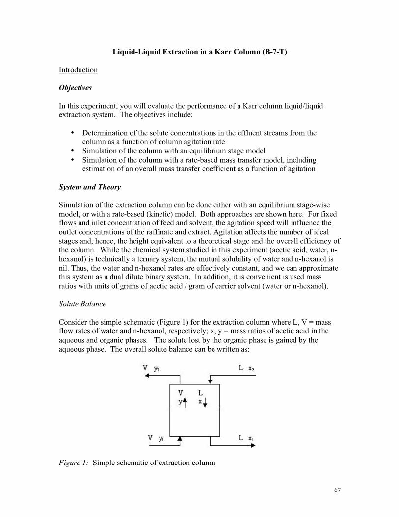
67

Liquid-Liquid Extraction in a Karr Column (B-7-T) Introduction Objectives In this experiment, you will evaluate the performance of a Karr column liquid/liquid extraction system. The objectives include:

• Determination of the solute concentrations in the effluent streams from the column as a function of column agitation rate

• Simulation of the column with an equilibrium stage model • Simulation of the column with a rate-based mass transfer model, including

estimation of an overall mass transfer coefficient as a function of agitation System and Theory Simulation of the extraction column can be done either with an equilibrium stage-wise model, or with a rate-based (kinetic) model. Both approaches are shown here. For fixed flows and inlet concentration of feed and solvent, the agitation speed will influence the outlet concentrations of the raffinate and extract. Agitation affects the number of ideal stages and, hence, the height equivalent to a theoretical stage and the overall efficiency of the column. While the chemical system studied in this experiment (acetic acid, water, n-hexanol) is technically a ternary system, the mutual solubility of water and n-hexanol is nil. Thus, the water and n-hexanol rates are effectively constant, and we can approximate this system as a dual dilute binary system. In addition, it is convenient is used mass ratios with units of grams of acetic acid / gram of carrier solvent (water or n-hexanol). Solute Balance Consider the simple schematic (Figure 1) for the extraction column where L, V = mass flow rates of water and n-hexanol, respectively; x, y = mass ratios of acetic acid in the aqueous and organic phases. The solute lost by the organic phase is gained by the aqueous phase. The overall solute balance can be written as:

Figure 1: Simple schematic of extraction column

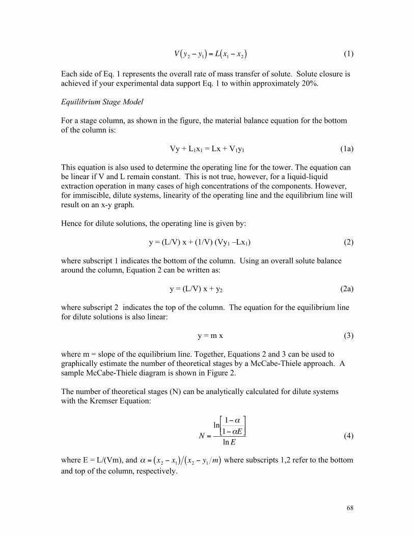
68

!

V y2" y

1( ) = L x1" x

2( ) (1) Each side of Eq. 1 represents the overall rate of mass transfer of solute. Solute closure is achieved if your experimental data support Eq. 1 to within approximately 20%. Equilibrium Stage Model For a stage column, as shown in the figure, the material balance equation for the bottom of the column is:

Vy + L1x1 = Lx + V1y1 (1a) This equation is also used to determine the operating line for the tower. The equation can be linear if V and L remain constant. This is not true, however, for a liquid-liquid extraction operation in many cases of high concentrations of the components. However, for immiscible, dilute systems, linearity of the operating line and the equilibrium line will result on an x-y graph. Hence for dilute solutions, the operating line is given by:

y = (L/V) x + (1/V) (Vy1 –Lx1) (2) where subscript 1 indicates the bottom of the column. Using an overall solute balance around the column, Equation 2 can be written as:

y = (L/V) x + y2 (2a)

where subscript 2 indicates the top of the column. The equation for the equilibrium line for dilute solutions is also linear:

y = m x (3) where m = slope of the equilibrium line. Together, Equations 2 and 3 can be used to graphically estimate the number of theoretical stages by a McCabe-Thiele approach. A sample McCabe-Thiele diagram is shown in Figure 2. The number of theoretical stages (N) can be analytically calculated for dilute systems with the Kremser Equation:

!

N =

ln1"#

1"#E

$

% & '

( )

lnE (4)

where E = L/(Vm), and

!

" = x2# x

1( ) x2# y

1m( ) where subscripts 1,2 refer to the bottom

and top of the column, respectively.

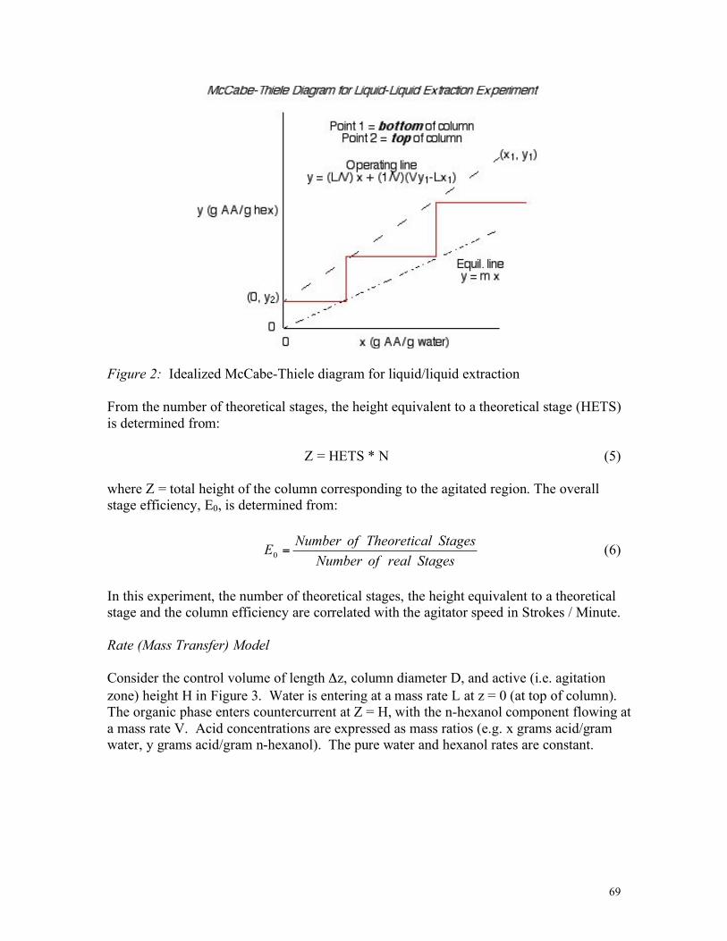
69

Figure 2: Idealized McCabe-Thiele diagram for liquid/liquid extraction From the number of theoretical stages, the height equivalent to a theoretical stage (HETS) is determined from:

Z = HETS * N (5) where Z = total height of the column corresponding to the agitated region. The overall stage efficiency, E0, is determined from:

StagesrealofNumber

StageslTheoreticaofNumberE =0

(6)

In this experiment, the number of theoretical stages, the height equivalent to a theoretical stage and the column efficiency are correlated with the agitator speed in Strokes / Minute. Rate (Mass Transfer) Model Consider the control volume of length Δz, column diameter D, and active (i.e. agitation zone) height H in Figure 3. Water is entering at a mass rate L at z = 0 (at top of column). The organic phase enters countercurrent at Z = H, with the n-hexanol component flowing at a mass rate V. Acid concentrations are expressed as mass ratios (e.g. x grams acid/gram water, y grams acid/gram n-hexanol). The pure water and hexanol rates are constant.

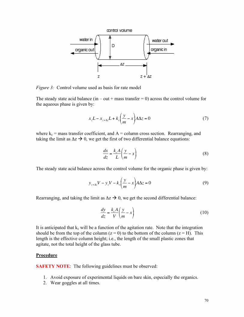
70

Figure 3: Control volume used as basis for rate model The steady state acid balance (in – out + mass transfer = 0) across the control volume for the aqueous phase is given by:

!

xzL " xz+#zL + kcy

m" x

$

% &

'

( ) A#z = 0 (7)

where kc = mass transfer coefficient, and A = column cross section. Rearranging, and taking the limit as Δz 0, we get the first of two differential balance equations:

!

dx

dz=kcA

L

y

m" x

#

$ %

&

' ( (8)

The steady state acid balance across the control volume for the organic phase is given by:

!

yz+"zV # yzV # kcy

m# x

$

% &

'

( ) A"z = 0 (9)

Rearranging, and taking the limit as Δz 0, we get the second differential balance:

!

dy

dz=kcA

V

y

m" x

#

$ %

&

' ( (10)

It is anticipated that kc will be a function of the agitation rate. Note that the integration should be from the top of the column (z = 0) to the bottom of the column (z = H). This length is the effective column height; i.e., the length of the small plastic zones that agitate, not the total height of the glass tube. Procedure SAFETY NOTE: The following guidelines must be observed:

1. Avoid exposure of experimental liquids on bare skin, especially the organics. 2. Wear goggles at all times.

71

3. Do NOT flood the column by excessive agitation. 4. Make sure all column effluent streams flow into the large round glass vessels. 5. Do NOT drain any fluids directly into the floor drain. The instructor is

responsible for draining the large glass spheres. 6. Do NOT try to pump the contents of the waste organic tank back to the feed tank.

Column Operation Note: The existing feed pump (on the floor) for both organic and water phases has

failed. We will use the pump that transfers fresh organic from the large steel storage tank to the glass sphere as the organic feed pump to the column. The instructor will explain the temporary rig currently in place. House water is now fed directly through a pressure regulator, then the water flow meter, and then into the column, thus bypassing the failed water pump. The water pressure regulator is set to deliver sufficient (~ 5 psig) of water to the experiment.

Note: In this experiment, “heavy” refers to the aqueous stream or phase and “light”

refers to the organic stream or phase.

1. Open the valve under the fresh organic steel storage tank that feeds the pump on the wall. If the tank is empty or very low, consult with the instructor. Do NOT open the valve that empties the tank onto the floor! Make sure the white recycle tube from the front of the experiment is sticking into the steel feed organic tank.

2. Turn on the organic feed pump near the floor on the wall behind the steel organic tank.

3. Using the two black-handled valves on the organic feed line near the front of the

experiment, fill the column with fresh organic phase; then stop the organic flow, and turn off the organic pump.

4. Admit water into the top of the column. Observe the water falling through the

organic phase, and then coalescing at the bottom of the column. Use the extract (heavy outlet) valve to manually maintain this interface below the inlet point of the fresh organic phase during the experiment. Use the white markers on the column as a guide. In this way, the water is the dispersed phase (i.e. bubbles), while the hexanol is the continuous phase. The water droplets fall through the agitated zone, and then coalesce at the base of the column.

5. Activate both the fresh water and fresh organic streams, and adjust to a flow rate

of 1 gallon per hour for each. Note that the flow meters are calibrated for water. A correction for the organic volumetric flow rate will be made.

6. Turn on the mechanical agitator using the switch located on the back wall. Also

turn on the neighboring switch to activate the digital agitator speed display.

72

7. Starting with a low agitator speed, make six runs at increasing agitation rates until flooding almost occurs. Flooding is observed when the column contents begin to get milky and the single interface at the base of the column appears with an interface at the top of the column. Do not flood the column! Adjust the agitation rate by turning the vertical shaft mounted about eye level with a flexible cable up to the agitator drive motor.

8. When steady state is reached (about 15 minutes at a total flow of about 2 gph),

sample the fresh organic, raffinate, and extract streams. Repeat this procedure for each agitation rate.

Sample Analyses Note: Make sure you locate the sampling points for the raffinate, extract, and the organic feed. Do not sample the organic feed from the feed tank. Also, the titration (see below) color change is clear-to-pink.

1. For the extract, titrate with standard 0.1N NaOH solutions using 10 drops of phenolphthalein as indicator. The end point occurs when the pink color lasts for about 30 seconds. Analytical solutions are available in the analytical room at the far end of the lab near the boiler room.

2. For organic samples, mix a 25 ml aliquot of sample with 75 ml of distilled water in

an extraction flask. Agitate vigorously to extract the acid from the organic phase into the distilled water. Wait a few minutes for the aqueous and organic phases to separate. Drain the aqueous phase into a beaker, and then titrate it as above.

3. Analyze the organic feed stream once before the first run, and again after the last

run of the column. The acetic acid concentrations you obtain should be similar. Also, these values should be similar to the concentration noted on the feed tank. If not, consult with the instructor.

System Shutdown

1. Make sure all flows and the agitator are turned off. 2. Carefully drain the column through the bottom valve into a convenient glass container. 3. Pour the column contents into the large stainless steel organic waste tank.

Data Analysis and Discussion

1. Plot the experimental raffinate and extract concentrations as functions of agitation rate. 2. For each run (i.e. for each agitation rate), perform the following analyses:

a. Tabulate each side of the solute balance (Eq. 1). If the differences are within ~ 20%, proceed with the next step. If not, consult the instructor.

b. Construct a McCabe-Thiele plot, and graphically estimate the number of theoretical stages.

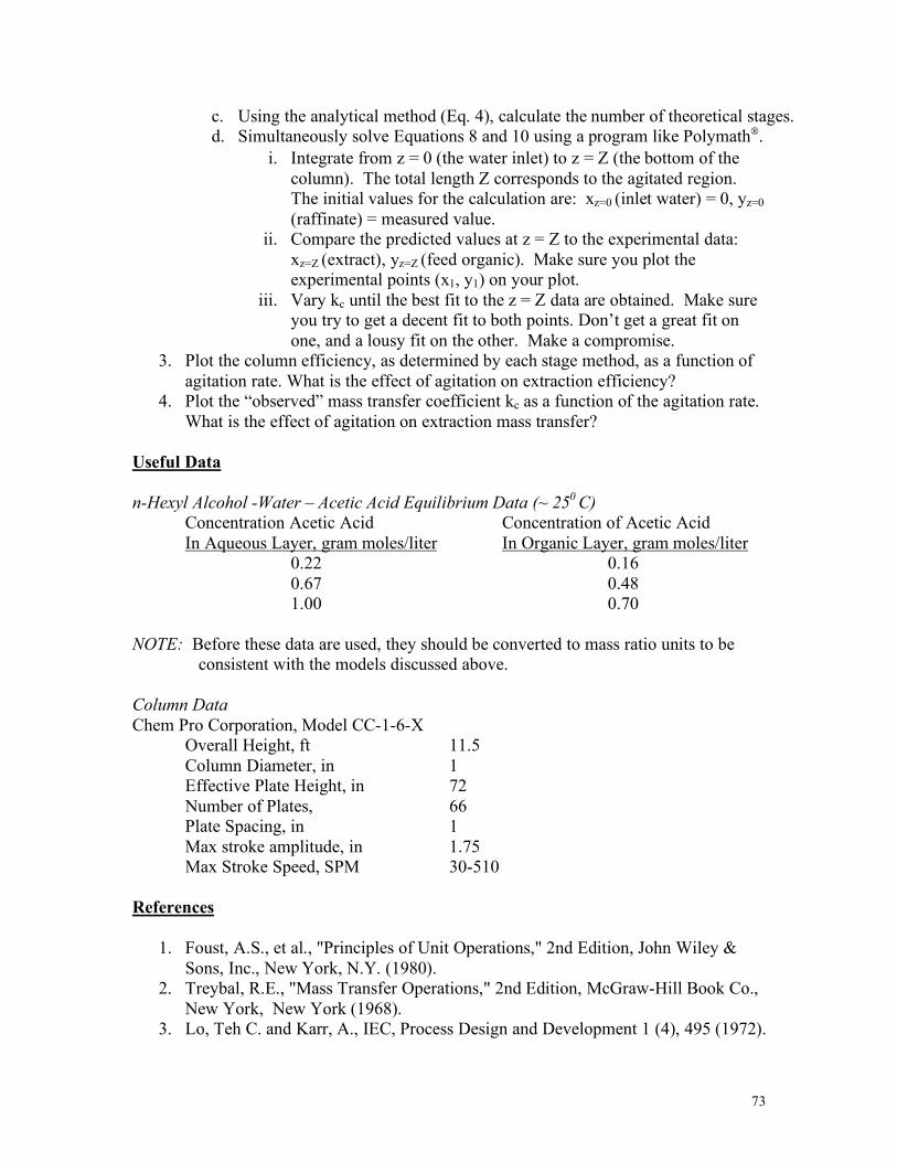
73

c. Using the analytical method (Eq. 4), calculate the number of theoretical stages. d. Simultaneously solve Equations 8 and 10 using a program like Polymath.

i. Integrate from z = 0 (the water inlet) to z = Z (the bottom of the column). The total length Z corresponds to the agitated region. The initial values for the calculation are: xz=0 (inlet water) = 0, yz=0 (raffinate) = measured value.

ii. Compare the predicted values at z = Z to the experimental data: xz=Z (extract), yz=Z (feed organic). Make sure you plot the experimental points (x1, y1) on your plot.

iii. Vary kc until the best fit to the z = Z data are obtained. Make sure you try to get a decent fit to both points. Don’t get a great fit on one, and a lousy fit on the other. Make a compromise.

3. Plot the column efficiency, as determined by each stage method, as a function of agitation rate. What is the effect of agitation on extraction efficiency?

4. Plot the “observed” mass transfer coefficient kc as a function of the agitation rate. What is the effect of agitation on extraction mass transfer?

Useful Data n-Hexyl Alcohol -Water – Acetic Acid Equilibrium Data (~ 250 C)

Concentration Acetic Acid Concentration of Acetic Acid In Aqueous Layer, gram moles/liter In Organic Layer, gram moles/liter

0.22 0.16 0.67 0.48 1.00 0.70

NOTE: Before these data are used, they should be converted to mass ratio units to be

consistent with the models discussed above. Column Data Chem Pro Corporation, Model CC-1-6-X

Overall Height, ft 11.5 Column Diameter, in 1 Effective Plate Height, in 72 Number of Plates, 66 Plate Spacing, in 1 Max stroke amplitude, in 1.75 Max Stroke Speed, SPM 30-510

References

1. Foust, A.S., et al., "Principles of Unit Operations," 2nd Edition, John Wiley & Sons, Inc., New York, N.Y. (1980).

2. Treybal, R.E., "Mass Transfer Operations," 2nd Edition, McGraw-Hill Book Co., New York, New York (1968).

3. Lo, Teh C. and Karr, A., IEC, Process Design and Development 1 (4), 495 (1972).

74

OPTICAL METHODS FOR BATCH REACTOR (311 T)

Introduction Objectives In this experiment, you will use optical methods to evaluate a chemical process in a batch reactor. There are two major parts to this experiment. Part I: Reaction Kinetics in a Homogeneous Solution -- household bleach (NaOCl active

ingredient) + blue food color (erioglaucine) – where one reagent is in excess. This part should establish the reaction kinetic orders and the rate constant.

Part II: Impact of Temperature – same system as Part I, except temperature will be

varied to estimate the Arrhenius parameters. Simple Light Interaction with Solutions When light passes through a fluid, the e/m wave interacts with the fluid molecules and anything particles in the fluid. If absorption and/or scattering of the light by the molecules and/or particles occurs, the transmitted intensity of the e/m wave is attenuated. The transmitted intensity It is given by the Beer-Lambert law:

!

It

= Ioexp "#CL( ) (1)

where Io = incident intensity, C = concentration of species (molecule or particle) that is absorbing and/or scattering the e/m wave concentration, L = optical path length, and σ = attenuation cross section that is usually a function of the e/m wavelength. Food color is a complex organic dye with a broad-banded absorption spectrum. Since we will use a Helium-Neon (He-Ne) laser at 632 nanometers (nm), the dye of choice is one with a spectrum with a reasonably strong absorption at the red 632 nm line; i.e., blue or green. Transmission of the beam through a volume of absorbing dye solution is governed by the Beer-Lambert law:

!

It

= Ioexp "#

ACDL( ) (1a)

where It = transmitted intensity, Io = incident intensity, σA = absorption cross section, CD = dye concentration, and L = optical path length (i.e. distance laser beam passes through dye solution). Typically, Eq. (1a) is rewritten as:

!

A " lnIo

It

#

$ %

&

' ( =)A

CDL (2)

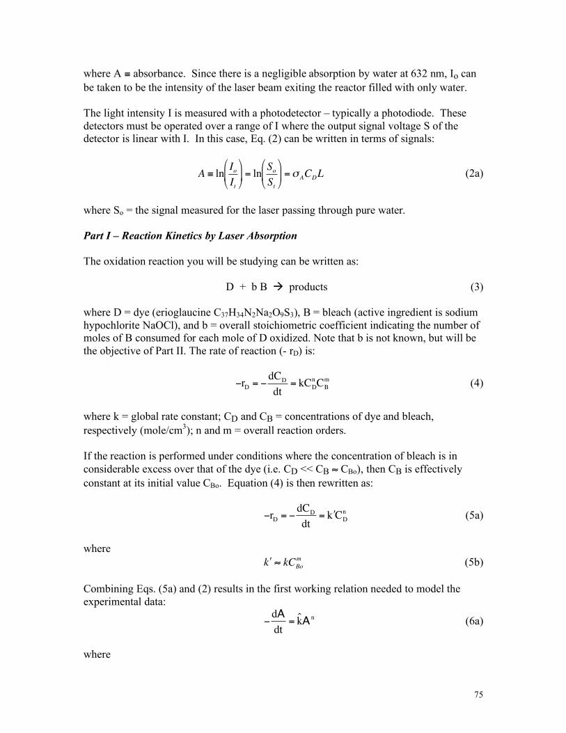
75

where A ≡ absorbance. Since there is a negligible absorption by water at 632 nm, Io can be taken to be the intensity of the laser beam exiting the reactor filled with only water. The light intensity I is measured with a photodetector – typically a photodiode. These detectors must be operated over a range of I where the output signal voltage S of the detector is linear with I. In this case, Eq. (2) can be written in terms of signals:

!

A " lnIo

It

#

$ %

&

' ( = ln

So

St

#

$ %

&

' ( =)A

CDL (2a)

where So = the signal measured for the laser passing through pure water. Part I – Reaction Kinetics by Laser Absorption The oxidation reaction you will be studying can be written as:

D + b B products (3) where D = dye (erioglaucine C37H34N2Na2O9S3), B = bleach (active ingredient is sodium hypochlorite NaOCl), and b = overall stoichiometric coefficient indicating the number of moles of B consumed for each mole of D oxidized. Note that b is not known, but will be the objective of Part II. The rate of reaction (- rD) is:

!

"rD

= "dC

D

dt= kC

D

nCB

m (4)

where k = global rate constant; CD and CB = concentrations of dye and bleach, respectively (mole/cm3); n and m = overall reaction orders. If the reaction is performed under conditions where the concentration of bleach is in considerable excess over that of the dye (i.e. CD << CB ≈ CBo), then CB is effectively constant at its initial value CBo. Equation (4) is then rewritten as:

!

"rD

= "dC

D

dt= # k C

D

n (5a)

where

!

" k # kCBo

m (5b) Combining Eqs. (5a) and (2) results in the first working relation needed to model the experimental data:

!

"dA

dt= ˆ k A

n (6a)

where

76

!

ˆ k " # k $AL( )

1%n (6b) and is approximately a constant for a given experiment with a specific amount of excess bleach. For each run you make, you must determine

!

ˆ k . Using an integral approach, you must first guess a value of n, then integrate Eq. (6a). If n = 1, then Eq. (6a) integrates to:

!

lnA

t= 0

At

"

# $

%

& ' = ˆ k t (7)

where At=o = the absorbance with water and dye present but before the bleach is added, and At = absorbance at any time t. If n not equal to 1, then Eq. (6a) integrates to:

!

A1-n = n "1( )ˆ k t + A

t= 0

1"n (8) Your absorbance data are correlated with either Eqs. (7) or (8) to determine the "best fit" reaction order n and the lumped rate constant

!

ˆ k . Eqs. (5b) and (6b) are combined to show that:

!

ˆ k = kCBo

m "AL( )

1#n (9) Assuming your values of n are about the same (use an average), the

!

ˆ k values from the runs with different volumes of excess bleach are then correlated with bleach concentrations using Eq. (9) to determine the "best fit" reaction order m. Taking the logarithm of Eq. (9) yields:

!

ln ˆ k ( ) = ln k "AL( )

1#n[ ] + m ln CBo( ) (10)

A plot of ln(

!

ˆ k ) vs. ln(CBo) according to Eq. (10) should yield a slope of m and the rate constant k to within a constant

!

"AL( )

1#n. If your value of n ≈ 1, k is determined directly.

Part II – Temperature Dependence Assume the rate constant k has an Arrhenius dependence on absolute temperature:

!"

#$%

& '=

RT

EAk A

f exp (11)

where Af = pre-exponential factor, EA = activation energy, R = ideal gas constant, and T = absolute temperature.

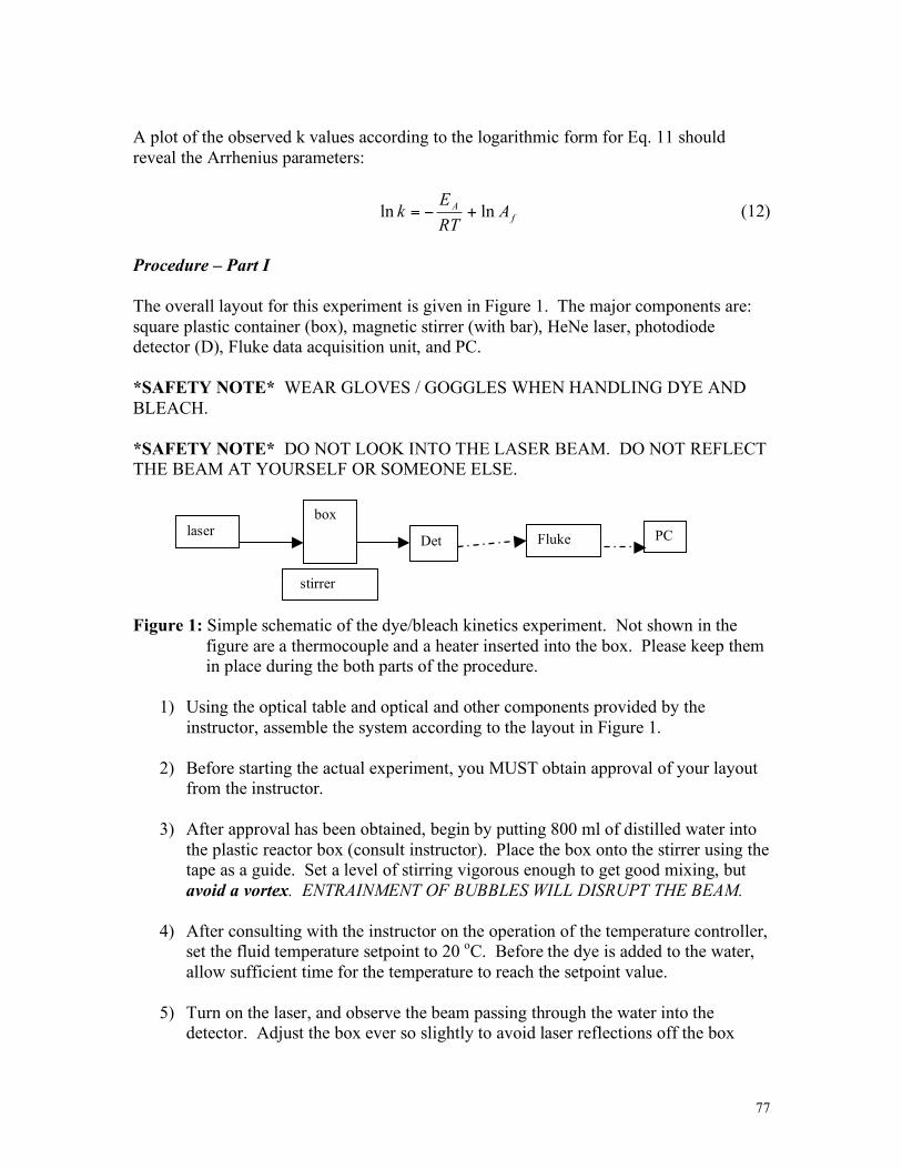
77

A plot of the observed k values according to the logarithmic form for Eq. 11 should reveal the Arrhenius parameters:

f

A ART

Ek lnln +!= (12)

Procedure – Part I The overall layout for this experiment is given in Figure 1. The major components are: square plastic container (box), magnetic stirrer (with bar), HeNe laser, photodiode detector (D), Fluke data acquisition unit, and PC. *SAFETY NOTE* WEAR GLOVES / GOGGLES WHEN HANDLING DYE AND BLEACH. *SAFETY NOTE* DO NOT LOOK INTO THE LASER BEAM. DO NOT REFLECT THE BEAM AT YOURSELF OR SOMEONE ELSE. Figure 1: Simple schematic of the dye/bleach kinetics experiment. Not shown in the

figure are a thermocouple and a heater inserted into the box. Please keep them in place during the both parts of the procedure.

1) Using the optical table and optical and other components provided by the

instructor, assemble the system according to the layout in Figure 1. 2) Before starting the actual experiment, you MUST obtain approval of your layout

from the instructor.

3) After approval has been obtained, begin by putting 800 ml of distilled water into the plastic reactor box (consult instructor). Place the box onto the stirrer using the tape as a guide. Set a level of stirring vigorous enough to get good mixing, but avoid a vortex. ENTRAINMENT OF BUBBLES WILL DISRUPT THE BEAM.

4) After consulting with the instructor on the operation of the temperature controller, set the fluid temperature setpoint to 20 oC. Before the dye is added to the water, allow sufficient time for the temperature to reach the setpoint value.

5) Turn on the laser, and observe the beam passing through the water into the

detector. Adjust the box ever so slightly to avoid laser reflections off the box

laser box

stirrer

Det Fluke PC

78

back into the laser. It’s OK to let the reflection hit the front of the laser housing. Make sure the laser beam hits the detector in the middle of the square (inside the circle). Use the corner of a business card or a piece of paper to help locate the beam if needed. Turn on the detector. Note the green “power on” light on top.

6) Carefully insert the thermocouple probe into the reactor box. Make sure the laser

beam does NOT hit the probe. In addition, insert the conductivity probe; but, it will not be used till Part 2 below.

7) Consult with the instructor about hooking up the detector signal wires to the Fluke

data logger. Make sure the Fluke is hooked up to the laptop using the GPIB/USB cable. Activate the Fluke.

8) Log onto the PC. If you have trouble, see the instructor. On the Desktop, open

the Data Logger folder. Activate the “Fluke Hydra Data Acquisition” Labview program. Review its operation with the instructor. Make sure you set the input channel to correspond to the optical detector in use. Set the program for “zero” time delay between samples.

NOTE: The dye solution to be used is the erioglaucine stock solution in the jug on the

bench behind the CSTR experiment in 311T. Currently, the solution concentration is 0.33 g/l. [If there is no more dye solution, coordinate with the CSTR group nearby, and make some new solution (at least a few liters)]. Withdraw a small amount in beaker. Use the small plastic syringe provided to dispense 1.25 ml of the dye into the reactor box (see instructor).

9) Begin a signal trace and data collection. Let the “clear water” signal trace for

about a minute. Then, using the syringe, carefully transfer the dye solution to the reactor box. Wait a few moments until the signal stabilizes. Note that there might be a small, but regular, oscillation in the signal. This is due to an oscillation in the laser intensity since the laser is old.

10) Without stopping the signal trace, transfer a known volume of bleach (e.g. 25 ml)

to the stirred reactor. Measure the signal until it stabilizes. Save your data trace to the desktop, and then to a floppy.

11) Turn off the variac (power to heater). Carefully move the thermocouple and heater to allow for removal of box. Stop the stirring, and wash out the box WELL in the sink. Don’t lose the magnetic stirrer down the drain!! Dry excess water off the sides and bottom of the box.

12) Repeat experiment (from step 2) with a new volume (same as previous run) of

distilled water and dye (same ml); however, change added bleach volume (e.g. 35 ml, 45 ml, 55 ml, 65 ml) – verify with instructor. Do five runs. Be consistent in your delivery of the 1.25ml of dye. Prior to starting each run, make sure the box

79

is carefully placed on top of the stirring platform such that the laser beam is hitting the center of the detector.

Procedure – Part II 1) Perform at least 4 additional runs using the same amounts of water, dye, and bleach.

The only variable is the temperature maintained. Cover a range of at least 40 oF.

2) Make sure the vessel is thoroughly washed out between runs. Get to the target temperature with the plain water. Then, add the dye, followed by the bleach.

Clean Up Make sure the vessel is clean, and that the laser, heater, etc. are turned off. IMPORTANT NOTE: The optical detector linearly converts the laser intensity I hitting it into a signal voltage V according to:

!

V = aI . To calculate absorbances, we can therefore use the signal voltages we collect; i.e.,

A = ln I

inIout

( ) = ln V! Vt

( ) where Vt = voltage at any time t, and V∞ = ultimate voltage that your trace finally reaches after bleach is added to dye/water. This should account for any loss of intensity due to inert materials in the bleach. The final signal should be close to signal voltage of pure water. If not, consult the instructor. Analysis Due to the scanning delay in the Fluke data logger, a simple correction is needed between actual (elapsed) time and the “Labview” time downloaded to your data spreadsheet. For one input channel, convert to actual time using:

(sec)*8807.0(sec) eLabviewtimrealtime = Following the analysis presented in the Theory for Part I above, use your data to estimate the kinetic orders for the reaction, and the rate constant at the prevailing temperature. Repeat the analyses for the runs at different temperatures. Regress the estimated k values according to Eq. 12.

Useful References Delgado, P., Kasko, A., Nappi, J., and Barat, R., "An Experiment in Applied Optics in Chemical Engineering: Determination of the Kinetics of the Oxidation of an Organic Dye," Chemical Engineering Education, vol. 32, no. 3, p. 174 (1998). Fogler, H. S. and N. M. Gurmen, Elements of Chemical Reaction Engineering, 4th ed., Prentice-Hall (2006).

80

Continuous Distillation (B-7-T)

Introduction Objectives In this experiment, you will evaluate the performance of a continuous distillation column separating a non-azeotropic binary mixture. The objectives include:

• Determination of the tray temperature and composition profiles along the column • Estimate the number of ideal stages to achieve the observed separation • Compare the actual separation to that predicted by a theoretical column model

McCabe-Thiele Method

The number of theoretical stages is calculated by using an x-y equilibrium composition diagram together with the McCabe-Thiele stage-wise graphical method. One assumes constant molal (equimolar) overflow between the feed inlet and the top tray and the feed inlet and the bottom tray (Ref. 1). This assumption is generally satisfied (Ref. 5) if:

1. The molar heats of vaporization of both species are approximately equal.

2. There are negligible heats of mixing, negligible heat losses, constant heat capacities of the liquid and vapor streams, negligible column pressure drop.

On an xy composition diagram, it can be shown (Ref. 1) that the operating line for the enriching (upper) section of the column is:

!

y =R

R +1x +

xD

R +1 (1)

It can also be shown that this line intersects the 45-degree diagonal on this diagram at xD. For the stripping section, below the feed plate, the operating line is given by:

!

y =L

Vx "

BxB

V (2)

It can also be shown that this line intersects the 45-degree diagonal on this diagram at xB. The intersection of the two operating lines defines the q line,

11 !!

!=

q

xx

q

qy F (3)

where q = the heat needed to vaporize 1 mol of feed at the entering condition divided by the molar latent heat of vaporization of the feed. It can be shown that the q-line intersects the 45-degree diagonal on this diagram at xF. The quantity q can be estimated by:

81

LV

FV

hH

hHq

!

!= (4)

In our case, the feed is a sub-cooled liquid (q >1). The enthalpies are given by:

!

hL = cp fTbp f

"To( ) (5a)

!

HV = xWfcpW Tdp f

"To( ) + #W[ ] + xM fcpM Tdp f

"To( ) + #M[ ] (5b)

!

hf = cp fTf "To( ) (5c)

where the heat capacity of the feed

!

cp fis a mole fraction weighted average for our binary

mixture. Eq. 5a estimates the enthalpy of the feed between the reference temperature To and the feed at its bubble point

!

Tbp fwhich is obtained from a Txy diagram. Eq. 5c

estimates the enthalpy of the feed between the reference temperature To and the feed temperature Tf. The reference can be taken as liquid water at 0o C. Eq. 5b estimates the enthalpy of the vapor, at the feed composition, at its dew point

!

Tdp f, determined with a

Txy diagram. The calculation assumes unmixed components at To each heated separately as liquids (use pure component heat capacities

!

cp j) to

!

Tdp f, each vaporized at this

temperature (use latent heats λj), then mixed (ref: Treybal).

The McCabe-Thiele method is constructed by:

1) Start with the x-y equilibrium figure. Add the 45o diagonal.

2) Draw the enriching section operating line (Eq. 1) using the experimental values for R and xD. The enriching line intersects the diagonal at xD.

3) Calculate the q value for your case using the experimental feed composition and temperature, with help from Eq. 5. Draw the q line according to Eq. 4. The q line intersects the diagonal at xF.

4) Draw the stripping section operating line (Eq. 2) by starting at the diagonal at the experimental bottoms composition xB, and running up to the intersection of the q line and enriching section line.

5) Starting at the xD point on the diagonal, step off stages between the operating and equilibrium lines. Continue stepping off stages until the xB point on the diagonal is reached.

Efficiencies

To determine the overall column efficiency for a given separation, the number of theoretical plates required is divided by number of actual plates:

82

actual

ltheoretica

overall

N

NEE ==

0 (6)

The number of theoretical plates = number of theoretical stages – the reboiler

The Murphree vapor efficiency per plate is defined by:

1

1

* +

+

!

!=

nn

nn

yy

yyEv (7)

Procedure

Overall Procedure

The overall procedural goal is to operate the column in a steady-state manner, achieving both non-zero distillate and bottoms flows, and a reasonable temperature spread across the column (bottom to top) for a steady feed flow rate. Samples will be collected for composition analysis, while a computerized log file records most other important data.

You should perform the pre-experimental ASPEN simulation before trying to run the column so as to get an estimate for what your column operation might look like. Most importantly, this simulation will give you an idea of a target steam rate and reflux ratio.

Control Loops

There are 6 control loops that are available in this system. Do not activate any of them yet until called for in the Startup section below. Some work, and some are not responsive. Read the following carefully.

I) Cold Water PID – When ON, this loop controls the cooling water flow rate through the condenser by monitoring the difference between the inlet and outlet cooling water temperatures of the condenser. Keep OFF. During normal operation, the condenser cooling water rate will be set manually at full flow rate, so that the cooling water picks up no more than a few oF passing through the condenser.

II) Bottoms Product PID – When ON, this loop maintains vapor integrity in the reboiler by keeping the sump at the bottom of the weir in the reboiler from running dry. This loop should be run with a set-point of ~ 4-5 inches of liquid. The bottoms pump must be ON as long as liquid is coming over the weir, and entering the sump. This loop should be used. NOTE: Keep an eye on the temperature of the steam condensate. There should be sufficient cooling water flow through the bottoms product cooler to also cool this condensate since the same cooling water does double duty.

III) Reflux PID – When OFF, the reflux ratio is a user-set constant value. The reflux valve at the top of the column opens and closes in a proportion that will be consistent with your reflux ratio choice. If the loop is ON, the reflux valve is

83

manipulated at a non-constant reflux such that a specific target tray temperature is maintained. Keep OFF; use the manual reflux ratio option – set your ratio.

Loops IV, V, and VI below all involve the manipulation of the valve controlling steam flow to the reboiler. If all of these loops are OFF, a user-specified % valve opening can be manually set. Consult your instructor as to how to control the steam flow.

IV) Steam Flow PID – When ON, this loop keeps a constant, user-specified, mass flow rate of steam to the reboiler. Keep OFF since we’re using another loop.

V) Plate Temperature PID – When ON, this loop allows the user to specify the temperature on a particular tray by manipulation of the steam rate. It is recommended (Kister, 1990) that temperature control be placed where there is the greatest temperature sensitivity in the vapor/liquid equilibrium. Consideration of the Txy diagram (see below) shows this region to be where methanol composition is lowest. Hence, we’ll try to maintain temperature on tray 1 (above the reboiler) at 185o F using this loop. See the instructor for control loop parameters.

VI) Differential Pressure PID – When ON, this loop tries to keep a constant, user-specified, differential pressure across the column by manipulating the steam rate. Keep OFF.

Pre-Start-up Planning

In order to facilitate your experiment, you need to run a simulation of your planned run using ASPEN.® I recommend running a simple two-component (MeOH, H2O) feed into the DSTWU column with the following inputs:

• Components: Methanol, Water • Property Method: your choice (e.g. Peng-Robinson, NRTL) • Feed: (estimated) 75oF; 15 psia; 0.4 mole fraction methanol, balance water; 1.6

liter/min. The feed composition data should be modified to reflect actual conditions. You should test the feed composition from the feed tank (using the refractometer – see instructions below), and use the correct value in the simulation.

• # of stages: Physically, the column has 10 sieve trays (stages). If we include the reboiler, this gives us 11 real stages. If we assume an ~ 50% tray efficiency, this means the column has about 5-6 ideal stages. Enter 5 in the simulation.

• Light Key: methanol (recovery 0.9); Heavy Key: water (recovery 0.05) – values estimated

• Condenser pressure: 14.7 psia; reboiler pressure: 15 psia (values estimated)

Once you generate simulated results, you should try to set the column parameters accordingly. Important results to consider include:

• Condenser heat duty: This value should be converted to a cooling water rate based on the inlet cooling water temperature (measured) and an assumed temperature rise of the cooling water of ~ 10-15 oF. Also, make sure the condenser temperature (hot vapor) is greater than your inlet cooling water temperature.

84

• Reboiler heat duty: This value should be converted to a steam rate assuming saturated steam at the measured inlet steam temperature. Make sure you use the steam flow rate calibration (see below). This is needed since the steam flow rate sensor is a bit out of calibration. The steam rate will be controlled by the loop. See if the steady state steam rate is close to that calculated by ASPEN.

• Reflux ratio: You can set the reflux ratio for the column operation with this value, or close to it.

Column Start-up

1. Move the PC mouse to light up the Distillation screen; the power should be always on. Make sure the visual of the system is active showing live temperatures and other data. If not, consult with the instructor.

2. Click on “Start Up”. The Screen will change to a Startup “tree” with “branches”. 3. Examine the level of the feed mixture tank. Drain both product tanks into the

feed tank. Then, open both valves from the product tanks to the feed tank. Then click on the most appropriate button. If the level is less than ½ full, consult with the instructor.

4. Examine the liquid level in the reboiler. If there is liquid visible through the reboiler window, then click on the Level Checked button. Otherwise, see the instructor.

5. Open the valve on the purge nitrogen gas cylinder. Adjust supply pressure to 10 psig. Consult with the instructor or TA for cylinder and regulator use and safety. Adjust the Nitrogen Purge Flowmeter attached to the cylinder regulator to 1.0 SCFH. Then click on the Nitrogen Purge System “Enabled” button.

6. Open the valve in the instrument air supply line located on the wall. Then click on Supply Air System “Enabled”.

7. Open the valve in the water supply line located on the wall. This supplies water to the Distillation Column condenser and bottoms product cooler. Make sure the product cooler valve is open. Then, click on Cooling Water System “Start”. Also, click on Cooling Water System Manual Mode “Start”. The condenser and bottoms product cooling water valves should be about 20% open. If not, see the instructor.

8. Set the Reflux Ratio at the desired value, then click on “Start”. 9. Click on your ASPEN-estimated Feed Point: “Upper”(Tray 7), “Middle” (Tray 5),

“Lower” (Tray 3). Remember to account for the stage efficiency. Also, count from the top. For example, if the estimated feed tray is 3, then the actual stage is 6. Click on Upper or Middle. If you choose the Upper location, see the instructor first. Do NOT turn on the feed pump yet, however.

10. Open the main steam valve by the wall. Initiate steam flow on the Startup tree. Jump to Home, and activate the steam control loop for maintaining a specific tray temperature. Set a desired 185o F for tray 1.

11. Adjust Condenser Water Flow. Click on the Cooling WaterValve on the flow diagram. In the box that opens, set the desired flow rate at a value at least what you estimated from the condenser duty based on the ASPEN simulation. Click on “OK”.

85

12. Click on “Start” for Feed Flow Valve. Then, “Start” the Feed Pump. Jump back to Home. Click on the Feed line, and set the “100% Open” value under the feed pump. The resulting flow rate should be ~ 1.6 liters/min.

13. Click on the Bottoms Product PID. Click this loop ON. Turn on the bottoms pump once you see the liquid level in the bottoms sump exceeding the 4 inch setpoint.

14. Monitor the column operation, and look for a steady state. Look for: a. A decent temperature spread (~150 oF at the top to ~190 oF in reboiler) b. Bottoms and distillate flow c. Ask the instructor to examine your column operation.

15. Once steady state is achieved, begin taking samples of vapor and liquid from the stages. Don’t forget to sample the feed tank liquid, and the top and bottoms products from the column. Consult the instructor for evaluation of your column operation.

16. The column operation might drift slowly over time due to a couple of possible reasons. For example, a higher drifting reboiler temperature, at the same steam rate, probably indicates a shifting composition in the reboiler. Your best bet is to keep an eye on the clear glass section (on first floor, visible from bottom floor through grate). You should target about 1-2” of boiling liquid. Observe the differential pressure drop across the column. Adjust the steam rate to maintain a value about ~6-8” water.

Sample Collection

1. Make sure the column is running at steady state, as judged by its temperature profile, boilup, and column differential pressure.

2. Make sure the sample condensers (coffee cans) are filled with ice water. Ice is available in the ChE stockroom – ask the TA or the instructor for help.

3. Blow out the sample condensation coil with compressed air before each new sample. Air guns are available on both floors near the column.

4. Collect liquid and vapor samples from each tray. Let the chilled liquid flow out of the small sample coil into a waste container for about 10 seconds before a good sample is directed into a small, labeled glass jar with sealing cap. This technique purges the sample cooling coil to avoid cross-contamination.

Sample Composition Analysis

1. A refractometer will be used to determine composition of your samples. Before the first sample, make sure the circulating constant temperature bath is set to Medium. Then, turn on the cooling water to a strong flow (the water drains into the nearby sink). Make sure the thermometer reads ~ 25oC. The analysis procedure is as follows:

a. Open up the prisms, and make sure the surfaces are clean. b. Using an eyedropper, place a few milliliters of liquid on the lower prism.

Close the prism assembly. c. Turn on the light source, and swing it up to illuminate the prisms. d. Looking through the eyepiece, note two zones (dark, light) with a

horizontal interface between them. Adjust the front horizontal dial to sharpen this interface.

86

e. Turn the large knob on the back, right side until the interface moves directly on top of a pair of cross-haired lines.

f. Press and hold the button on the back, left side. Carefully read the refractive index to 4 decimal places.

g. Open up the prism assembly. Wipe the prism surfaces dry with lens tissue or a soft cloth. Avoid using paper towels – they are too coarse.

h. Review the operation with the instructor. 2. Prior to sample analyses with the refractometer, verify its operation by measuring

the refractive indices of pure distilled water and pure methanol. For consistency, it is recommended that the same person in your group do all the samples.

3. Be especially attentive to the analyses of the feed, distillate, and bottoms samples.

Electronic Data Collection

1. Logging In

a. Click “START” in the “Logging” box. b. Fill in all necessary information, such as Course, Course Number, Names,

etc. Use the “tab” key to save your entries and move between entries. c. Click “START LOGGING”. d. Click “OK” to confirm.

2. Logging Out and Retrieving Data

a. Insert a floppy disk into the PC (see the instructor if you don’t have one). b. Under “Logging,” click “STOP”. c. Click “Stop Logging” – answer the pop-up question “yes”. d. Click “COPY” to change the file name to the same as student’s names or

to modify the file name as desired. e. Click “CREATE REPORT” to create report file (wait around five seconds). f. Click “OPEN REPORT”. A window will open. Find your file, click once

on its name, then click “Open” to view the file in Excel. g. Go to File, then “Save As” this file to the floppy disk. h. Close this file, exit Excel, and then close the Logging dialog box. i. A useful key to the labels over each column of the Log file is presented at

the very end of this chapter.

Shutdown

1. Click on “Startup” to bring on the startup screen. Then in REVERSE ORDER, click on all “Stop” buttons going up the tree branches. Turning off the feed pump and the steam flow should be the first things you do.

2. Make sure you consult the posted “Shutdown Check List”, and close or turn off what is required.

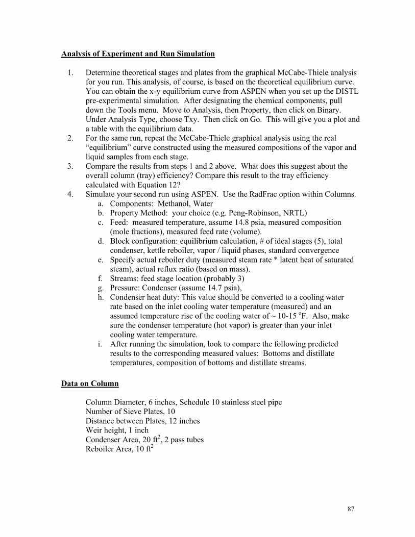
87

Analysis of Experiment and Run Simulation

1. Determine theoretical stages and plates from the graphical McCabe-Thiele analysis for you run. This analysis, of course, is based on the theoretical equilibrium curve. You can obtain the x-y equilibrium curve from ASPEN when you set up the DISTL pre-experimental simulation. After designating the chemical components, pull down the Tools menu. Move to Analysis, then Property, then click on Binary. Under Analysis Type, choose Txy. Then click on Go. This will give you a plot and a table with the equilibrium data.

2. For the same run, repeat the McCabe-Thiele graphical analysis using the real “equilibrium” curve constructed using the measured compositions of the vapor and liquid samples from each stage.

3. Compare the results from steps 1 and 2 above. What does this suggest about the overall column (tray) efficiency? Compare this result to the tray efficiency calculated with Equation 12?

4. Simulate your second run using ASPEN. Use the RadFrac option within Columns. a. Components: Methanol, Water b. Property Method: your choice (e.g. Peng-Robinson, NRTL) c. Feed: measured temperature, assume 14.8 psia, measured composition

(mole fractions), measured feed rate (volume). d. Block configuration: equilibrium calculation, # of ideal stages (5), total

condenser, kettle reboiler, vapor / liquid phases, standard convergence e. Specify actual reboiler duty (measured steam rate * latent heat of saturated

steam), actual reflux ratio (based on mass). f. Streams: feed stage location (probably 3) g. Pressure: Condenser (assume 14.7 psia), h. Condenser heat duty: This value should be converted to a cooling water

rate based on the inlet cooling water temperature (measured) and an assumed temperature rise of the cooling water of ~ 10-15 oF. Also, make sure the condenser temperature (hot vapor) is greater than your inlet cooling water temperature.

i. After running the simulation, look to compare the following predicted results to the corresponding measured values: Bottoms and distillate temperatures, composition of bottoms and distillate streams.

Data on Column Column Diameter, 6 inches, Schedule 10 stainless steel pipe Number of Sieve Plates, 10 Distance between Plates, 12 inches Weir height, 1 inch Condenser Area, 20 ft2, 2 pass tubes Reboiler Area, 10 ft2

88

Nomenclature

B = L-phase product; lb/h or lb-moles/h, kg/h or kg-moles/hr D = V-phase product; lb/h or lb-moles/h, kg/hr or kg-moles/h E = Murphree plate efficiency or Overall tray efficiency F = Feed; lb/h or lb-moles/h, kg/h or kg-moles/h H = Vapor-phase enthalpy concentration; Btu (lb or lb-moles), Cal/gm or cal/gm

mole, kJ/kg or kJ/(kg-moles) h = Liquid-phase enthalpy concentration; BTU (lb or lb- moles), cal/gm or cal/gm

mole, kJ/kg or kJ/(kg-moles) L = Liquid; lb/h or lb-moles/h, kg/h or kg-moles/h N = Number of ideal stages q = Heat added or removed; BTU/hr, kJ/h R = Ref1ux ratio = Lo / D or Ln / D V = Vapor; lb/h or lb-mo1es/h x = Fraction of any component in phase L; mass or mole fraction y = Fraction of any component in phase V; mass or mole fraction

Subscripts

D = distillate n = nth stage in enriching section F = feed c = condenser m = mth stage in stripping section s = reboiler B = bottoms v = vapor

Superscript

* = equilibrium value

References

1. Geankopolis, C. J., “Transport Processes and Separation Principles (Includes Unit Operations)”, 4th Edition, Prentice Hall, Upper Saddle River, New Jersey (2003)

2. Foust, A.S., et. al., "Principles of Unit Operations," 2nd Edition, John Wiley & Sons" Inc., New York (1980).

3. Treybal, R.E., "Mass Transfer Operations," 2nd Edition, McGraw-Hil1 Book Co., New York (1968).

4. McCabe, W.L., Smith, J. C. and Harriot, P., “Unit Operations of Chemical Engineering”, 5th Edition, McGraw-Hill Inc., New York (1993)

5. Seader, J. D. and Henley, E. J., “Separation Process Principles”, John Wiley and Sons, Inc., New York (1998).

6. Kister, H. Z., “Distillation Operation,” McGraw-Hill, NY (1990).

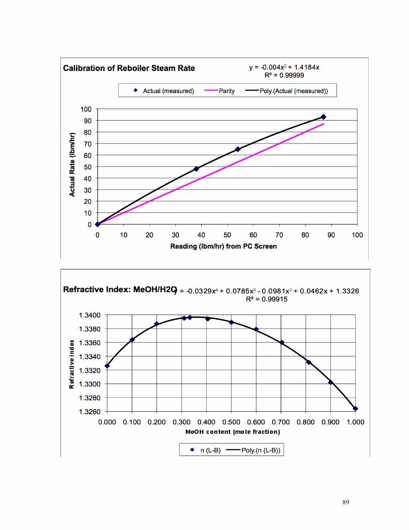
89

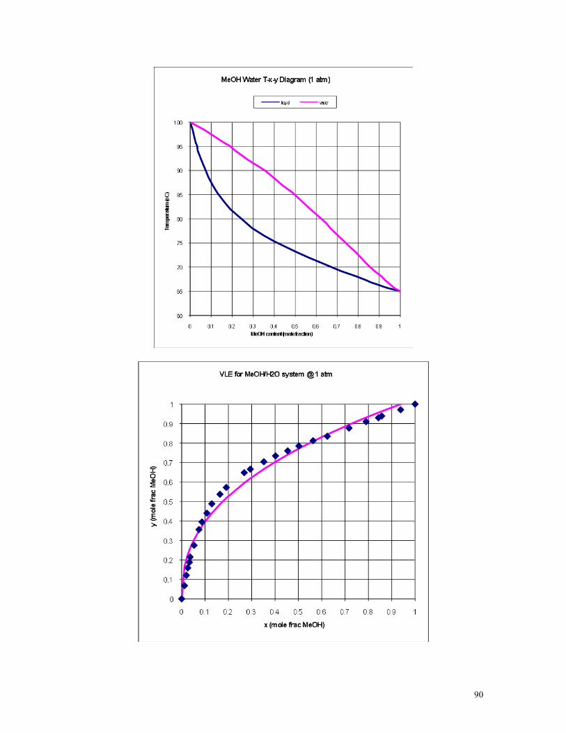
90

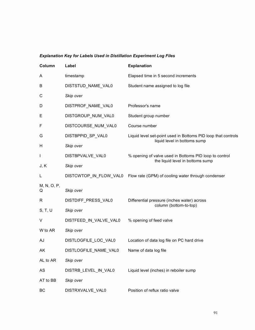
91

Explanation Key for Labels Used in Distillation Experiment Log Files Column Label Explanation A timestamp Elapsed time in 5 second increments B DISTSTUD_NAME_VAL0 Student name assigned to log file C Skip over D DISTPROF_NAME_VAL0 Professor's name E DISTGROUP_NUM_VAL0 Student group number F DISTCOURSE_NUM_VAL0 Course number G DISTBPPID_SP_VAL0 Liquid level set-point used in Bottoms PID loop that controls liquid level in bottoms sump H Skip over I DISTBPVALVE_VAL0 % opening of valve used in Bottoms PID loop to control the liquid level in bottoms sump J, K Skip over L DISTCWTOP_IN_FLOW_VAL0 Flow rate (GPM) of cooling water through condenser M, N, O, P, Q Skip over R DISTDIFF_PRESS_VAL0 Differential pressure (inches water) across column (bottom-to-top) S, T, U Skip over V DISTFEED_IN_VALVE_VAL0 % opening of feed valve W to AR Skip over AJ DISTLOGFILE_LOC_VAL0 Location of data log file on PC hard drive AK DISTLOGFILE_NAME_VAL0 Name of data log file AL to AR Skip over AS DISTRB_LEVEL_IN_VAL0 Liquid level (inches) in reboiler sump AT to BB Skip over BC DISTRXVALVE_VAL0 Position of reflux ratio valve

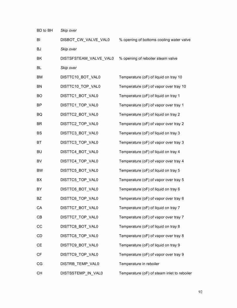
92

BD to BH Skip over BI DISBOT_CW_VALVE_VAL0 % opening of bottoms cooling water valve BJ Skip over BK DISTSFSTEAM_VALVE_VAL0 % opening of reboiler steam valve BL Skip over BM DISTTC10_BOT_VAL0 Temperature (oF) of liquid on tray 10 BN DISTTC10_TOP_VAL0 Temperature (oF) of vapor over tray 10 BO DISTTC1_BOT_VAL0 Temperature (oF) of liquid on tray 1 BP DISTTC1_TOP_VAL0 Temperature (oF) of vapor over tray 1 BQ DISTTC2_BOT_VAL0 Temperature (oF) of liquid on tray 2 BR DISTTC2_TOP_VAL0 Temperature (oF) of vapor over tray 2 BS DISTTC3_BOT_VAL0 Temperature (oF) of liquid on tray 3 BT DISTTC3_TOP_VAL0 Temperature (oF) of vapor over tray 3 BU DISTTC4_BOT_VAL0 Temperature (oF) of liquid on tray 4 BV DISTTC4_TOP_VAL0 Temperature (oF) of vapor over tray 4 BW DISTTC5_BOT_VAL0 Temperature (oF) of liquid on tray 5 BX DISTTC5_TOP_VAL0 Temperature (oF) of vapor over tray 5 BY DISTTC6_BOT_VAL0 Temperature (oF) of liquid on tray 6 BZ DISTTC6_TOP_VAL0 Temperature (oF) of vapor over tray 6 CA DISTTC7_BOT_VAL0 Temperature (oF) of liquid on tray 7 CB DISTTC7_TOP_VAL0 Temperature (oF) of vapor over tray 7 CC DISTTC8_BOT_VAL0 Temperature (oF) of liquid on tray 8 CD DISTTC8_TOP_VAL0 Temperature (oF) of vapor over tray 8 CE DISTTC9_BOT_VAL0 Temperature (oF) of liquid on tray 9 CF DISTTC9_TOP_VAL0 Temperature (oF) of vapor over tray 9 CG DISTRB_TEMP_VAL0 Temperature in reboiler CH DISTSSTEMP_IN_VAL0 Temperature (oF) of steam inlet to reboiler

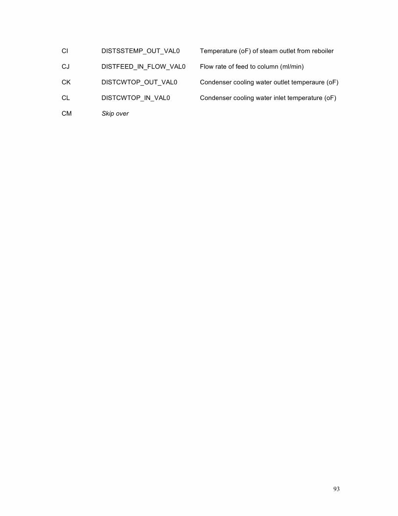
93

CI DISTSSTEMP_OUT_VAL0 Temperature (oF) of steam outlet from reboiler CJ DISTFEED_IN_FLOW_VAL0 Flow rate of feed to column (ml/min) CK DISTCWTOP_OUT_VAL0 Condenser cooling water outlet temperaure (oF) CL DISTCWTOP_IN_VAL0 Condenser cooling water inlet temperature (oF) CM Skip over

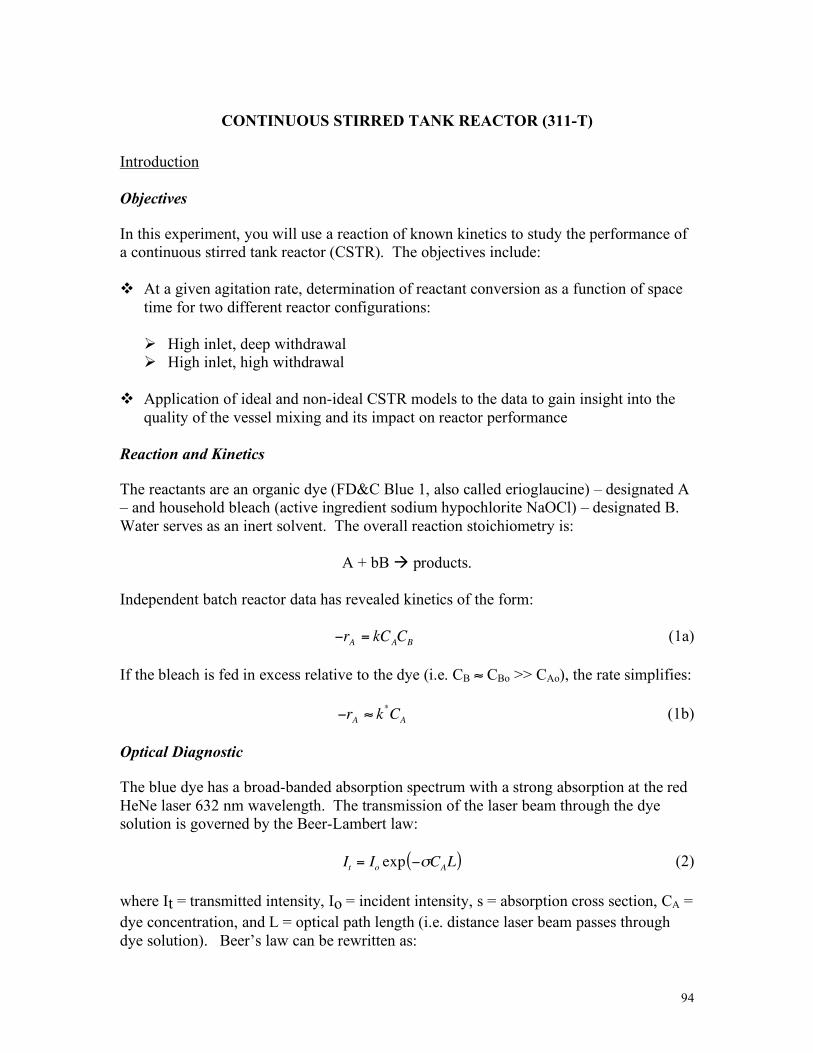
94

CONTINUOUS STIRRED TANK REACTOR (311-T) Introduction Objectives

In this experiment, you will use a reaction of known kinetics to study the performance of a continuous stirred tank reactor (CSTR). The objectives include: At a given agitation rate, determination of reactant conversion as a function of space

time for two different reactor configurations:

High inlet, deep withdrawal High inlet, high withdrawal

Application of ideal and non-ideal CSTR models to the data to gain insight into the

quality of the vessel mixing and its impact on reactor performance Reaction and Kinetics

The reactants are an organic dye (FD&C Blue 1, also called erioglaucine) – designated A – and household bleach (active ingredient sodium hypochlorite NaOCl) – designated B. Water serves as an inert solvent. The overall reaction stoichiometry is:

A + bB products. Independent batch reactor data has revealed kinetics of the form:

!rA= kC

ACB (1a)

If the bleach is fed in excess relative to the dye (i.e. CB ≈ CBo >> CAo), the rate simplifies:

!rA" k

*

CA (1b)

Optical Diagnostic

The blue dye has a broad-banded absorption spectrum with a strong absorption at the red HeNe laser 632 nm wavelength. The transmission of the laser beam through the dye solution is governed by the Beer-Lambert law:

It= I

oexp !"C

AL( ) (2)

where It = transmitted intensity, Io = incident intensity, s = absorption cross section, CA = dye concentration, and L = optical path length (i.e. distance laser beam passes through dye solution). Beer’s law can be rewritten as:

95

!

ˆ A " ln Io

It( ) =#C

AL (3)

where ˆ A = absorbance. Since there is no absorption by water at 632 nm, Io ≈ the intensity of the laser beam exiting the reactor filled with only water. Assuming the detector is operated linearly, the voltage signal Vt is directly proportional to It. This provides the working form of Beer’s Law:

ˆ A = ln Vo

Vt

( ) (4) Absorbance measurements are made using an optical flow cell located after the reactor. The flow cell can accept either the reactor effluent directly or an inlet bypass stream. Space Time and Conversion The space-time τ is given by:

!

" =V vwater + vdye + vbleach( ) (5) where V = CSTR liquid volume, and v = volumetric flow rate. Since absorbance ˆ A is directly proportional to dye concentration, dye conversion XA is given by:

!

XA

= ˆ A in" ˆ A

out( ) ˆ A in

(6) where

!

ˆ A in

corresponds to the total feed (dye, water, and bleach), and

!

ˆ A out

corresponds to the reactor effluent. The feed stream absorbance

!

ˆ A in

is estimated from the measured absorbance

!

ˆ A dye+water :

!

ˆ A in = ˆ A dye +water vwater + vdye( ) vwater + vdye + vbleach( ) (7) The absorbance

!

ˆ A dye+water is measured by bypassing the water + dye flow around the reactor and directing it right into the optical flow cell. The estimation in Eq. 7 is needed since combining the bleach with the water + dye flow would result in reaction. The assumption here is that the bleach has negligible absorbance at 632 nm, which has been independently confirmed. Ideal CSTR Model The single CSTR species balance is given by:

FAo! F

A+ r

A= 0 (8)

96

where FA = molar flow rate of A exiting the reactor, and subscript o indicates the inlet condition. Substituting the rate (Eq. 1b) and rearranging yields:

!

XA

= k*" 1+ k*"( ) (9) In the likely event that the bleach concentration was not maintained constant during the various runs as the total flow rate was changed, a more general form of Eq. 9 is recommended:

!

XA

=kC

Bo"

1+ kCBo"#

Da

1+ Da (10)

where Da = Damkohler number, which can be written as:

!

Da " kCBo# =

kCBo

1 # (11)

Notice that Da is a ratio of rates; specifically, a characteristic chemical rate divided by a characteristic flow rate. Procedure – Preparation

SAFETY NOTES: • Those handling the dye and bleach solutions should wear gloves in addition to goggles. • Avoid wearing better clothes or shoes. • Carefully study the experimental layout and its subsystems: flow control, reactor,

optical, data acquisition. • A laser is used in this experiment. DO NOT DIRECT THE BEAM INTO

ANYONE’S EYES! The beam is harmless to the skin. Dye Solution Preparation • Prepare ~ 1 liter of Erioglaucine dye solution at ~ 0.33 g/liter concentration (if not

already available on the adjacent bench). • Dissolve 0.33 g of dye in 1 liter of water with a magnet stirrer. • Remove the dye tank from its pedestal. • After prepared, carefully pour the tracer solution into the dye tracer tank. Take care

not to drop the magnetic stirred into the dye tank. • Prepare a total of 3 liters of dye solution. Carefully replace the dye tank onto its

pedestal. Reconnect the tubing; consult the instructor. • Set dye valve for recirculate to tank. Open dye supply valve. • Turn on dye pump, and recirculate dye back to tank with at a fairly high rate to verify

the dye flow system is working properly. • Once verified, turn off the dye pump.

97

Bleach Supply • Fill the bleach tank with Clorox to about ¾ full. Be careful not to spill it on yourself. • Set bleach bypass valve for return to tank. Open bleach supply valves. • Turn on bleach pump, and recirculate bleach back to the tank to verify this subsystem.

Do not flow bleach to the reactor yet! • Once verified, turn off the bleach pump. Prepare the Data Logger and PC 1) Activate the Fluke® data logger. Press the button until “Channel 5” is reached on

the display; hit “enter”. Hit the “function” button; then hit until “volts DC” is seen; then hit “enter”. When “AUTO” appears, hit “enter”. Finally, press the MON monitor button.

2) Make sure PC is activated. Log in (ignore password request), and get to Desktop. 3) Go into “Labview Stuff” folder. Activate theLabview “readvolts.vi” program. 4) Set the sampling time for 5 seconds. Set the interface switch to GPIB. Set to address 4. 5) Click on “enable trace”, but do not start the data collection yet. Optical System Preparation • Activate the HeNe laser. Verify beam alignment into the detector, and that the

detector is activated. Do this with water flowing through the optical flow cell. • If available, verify detector linearity by observing the Fluke reading with a 0.3 neutral

density filter (50 % transmission) held temporarily in front of the detector. Procedure – Reaction Studies

Note: A thermocouple and digital readout provide the reactor temperature. Record the temperature for each run.

Note: Study the piping layout of the entire system before you start flows. There are

numerous valves. Make sure you know the function of each valve! High Inlet, Deep Outlet • Begin with the configuration: High Inlet, Deep Outlet --- consult with the instructor. • Make sure the data collection program on the PC is ready to go and the Fluke is on. • Turn on the cold water supply, and begin an intermediate flow rate bypassing the

reactor and flowing directly through the optical cell. • Start data collection on the PC; make sure a live plot is on the screen. Observe the

“water only” baseline voltage signal. • Set the dye valve for recirculation back to the dye tank. Open dye supply valves. • Turn on the dye pump, and recirculate the dye back to the dye tank with at a fairly

low rate (~ 0.4 gph). • Redirect the dye flow to join the water, flowing both through the optical cell.

98

• Allow the signal trace to reach a steady state value. Estimate the

!

ˆ A dye+water value according to Eq. 4. Your target absorbance should be about 1.9 to 2, corresponding to a reduction in water-only baseline signal of ~ 85%. If the absorbance is considerably less, then either increase the dye flow rate or decrease the water rate.

• Set the vessel agitation rate at a moderate setting, but avoid entraining air bubbles. • With an acceptable

!

ˆ A dye+water , redirect the outlet valves for water + dye flow directly into the reactor, and total reactor effluent flow through the optical cell.

• Adjust the water and dye rotameters, if needed, to restore the flow rates used as bypass. • Allow the optical signal to achieve a new steady state value. This will take a while. • While waiting, set bleach bypass valve for return to tank. Open bleach supply valves. • Turn on bleach pump, and recirculate bleach back to the tank. Do not flow bleach to

the reactor yet! • Make sure the entire reactor effluent is flowing through the optical flow cell. • Once the signal has reached a steady state value, direct the bleach flow to the reactor

at an intermediate rate. This is your “t = 0” point. Wait for a new steady signal. • When the detector signal reaches a steady value, stop the bleach flow and redirect the

dye flow back to the dye tank. • When the trace reaches a steady value, stop the trace. Then save the data in a distinct

file (*.txt) onto the desktop (then a floppy). • Flush out the reactor until the signal returns to its baseline value. Use the effluent

bypass line to speed up the flush out. See the instructor. • Replenish the dye and bleach supply tanks as needed. • Repeat this entire sequence for a higher total flow rate while maintaining the same

feed concentrations of dye and bleach. Consult the instructor. Try to get a minimum of three runs at this reactor configuration.

High Inlet, High Outlet • Begin with the configuration: High Inlet, High Outlet --- consult with the instructor. • Repeat the above experiments for the SAME total flow rates. Try to get a minimum

of three runs at this reactor configuration. Procedure – Shutdown • Turn off all pumps and tank supply valves. • Flush water through the reactor until the contents are clear. • Shut down water supply. Data Analysis and Discussion 1) For each run, perform the following:

• Convert voltage signals to absorbances using Equation 4 • Calculate conversions using Equations 6 and 7

99

• Determine single ideal CSTR XA using Equation 10. Remember that CBo is based on the total flow into the reactor, not just the concentration of NaOCl (i.e. component B) in the bleach bottle.

• Plot experimental and model-based XA vs. Da. 2) What is the impact of the change in configuration? 3) Under what conditions does the reactor behave as a CSTR? Useful Data

k = 1.34E6 exp(-8800/R/T) liters/mole-second where R = 1.987 cal/mole-K, and T (K). The concentration of active ingredient NaOCl in household bleach is ~ 6 % (by weight). Check the bottle label to verify. The specific gravity of bleach is ~ 1.1. References

P. Delgado, A. Kasko, J. Nappi, and R. Barat, “An Experiment in Applied Optics: Determination of the Kinetics of the Oxidation of an Organic Dye,” Chemical Engineering Education, vol. 32, no. 3 (1998). Fogler and Gurmen, Elements of Chemical Reaction Engineering, 4th ed., Prentice-Hall (2004).

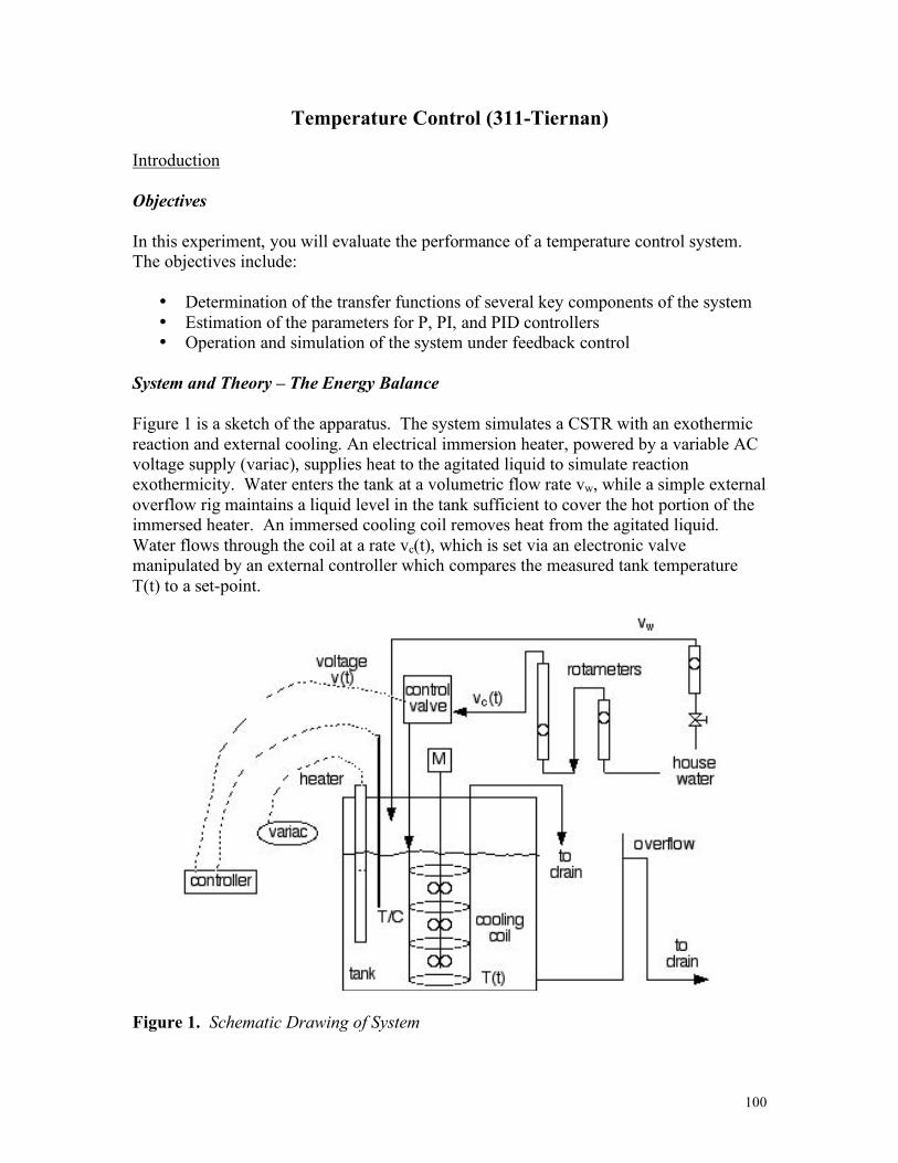
100

Temperature Control (311-Tiernan) Introduction Objectives In this experiment, you will evaluate the performance of a temperature control system. The objectives include:

• Determination of the transfer functions of several key components of the system • Estimation of the parameters for P, PI, and PID controllers • Operation and simulation of the system under feedback control

System and Theory – The Energy Balance Figure 1 is a sketch of the apparatus. The system simulates a CSTR with an exothermic reaction and external cooling. An electrical immersion heater, powered by a variable AC voltage supply (variac), supplies heat to the agitated liquid to simulate reaction exothermicity. Water enters the tank at a volumetric flow rate vw, while a simple external overflow rig maintains a liquid level in the tank sufficient to cover the hot portion of the immersed heater. An immersed cooling coil removes heat from the agitated liquid. Water flows through the coil at a rate vc(t), which is set via an electronic valve manipulated by an external controller which compares the measured tank temperature T(t) to a set-point.

Figure 1. Schematic Drawing of System

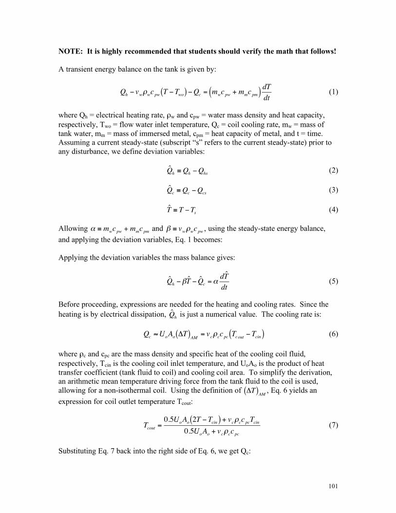
101

NOTE: It is highly recommended that students should verify the math that follows! A transient energy balance on the tank is given by:

!

Qh " vw#wcpw T "Two( ) "Qc = mwcpw + mmcpm( )dT

dt (1)

where Qh = electrical heating rate, ρw and cpw = water mass density and heat capacity, respectively, Two = flow water inlet temperature, Qc = coil cooling rate, mw = mass of tank water, mm = mass of immersed metal, cpm = heat capacity of metal, and t = time. Assuming a current steady-state (subscript “s” refers to the current steady-state) prior to any disturbance, we define deviation variables:

!

ˆ Q h "Qh #Qhs (2)

!

ˆ Q c"Q

c#Q

cs (3)

!

ˆ T " T #Ts (4)

Allowing

!

" # mwcpw + mmcpm and

!

" # vw$wcpw , using the steady-state energy balance, and applying the deviation variables, Eq. 1 becomes: Applying the deviation variables the mass balance gives:

!

ˆ Q h "#ˆ T " ˆ Q c =$

d ˆ T

dt (5)

Before proceeding, expressions are needed for the heating and cooling rates. Since the heating is by electrical dissipation,

!

ˆ Q h is just a numerical value. The cooling rate is:

!

Qc "UoAo #T( )AM

= vc$cc pc Tcout %Tcin( ) (6) where ρc and cpc are the mass density and specific heat of the cooling coil fluid, respectively, Tcin is the cooling coil inlet temperature, and UoAo is the product of heat transfer coefficient (tank fluid to coil) and cooling coil area. To simplify the derivation, an arithmetic mean temperature driving force from the tank fluid to the coil is used, allowing for a non-isothermal coil. Using the definition of

!

"T( )AM

, Eq. 6 yields an expression for coil outlet temperature Tcout:

!

Tcout =0.5UoAo 2T "Tcin( ) + vc#cc pcTcin

0.5UoAo + vc#cc pc (7)

Substituting Eq. 7 back into the right side of Eq. 6, we get Qc:

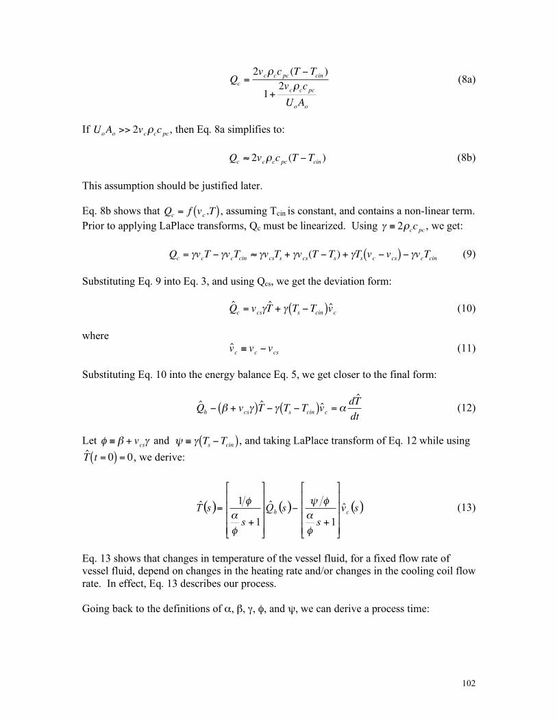
102

!

Qc =2vc"cc pc (T #Tcin )

1+2vc"cc pc

UoAo

(8a)

If

!

UoAo >> 2vc"cc pc, then Eq. 8a simplifies to:

!

Qc " 2vc#cc pc (T $Tcin ) (8b) This assumption should be justified later. Eq. 8b shows that

!

Qc = f vc,T( ) , assuming Tcin is constant, and contains a non-linear term. Prior to applying LaPlace transforms, Qc must be linearized. Using

!

" # 2$cc pc , we get:

!

Qc

= "vcT # "v

cTcin$ "v

csTs+ "v

cs(T #T

s) + "T

svc# v

cs( ) # "vcTcin (9)

Substituting Eq. 9 into Eq. 3, and using Qcs, we get the deviation form:

!

ˆ Q c

= vcs" ˆ T + " T

s#T

cin( ) ˆ v c (10)

where

!

ˆ v c" v

c# v

cs (11)

Substituting Eq. 10 into the energy balance Eq. 5, we get closer to the final form:

!

ˆ Q h " # + vcs$( ) ˆ T " $ Ts "Tcin( ) ˆ v c =%d ˆ T

dt (12)

Let

!

" # $ + vcs% and

!

" # $ Ts%T

cin( ), and taking LaPlace transform of Eq. 12 while using

!

ˆ T t = 0( ) = 0, we derive:

( ) ( ) ( )sv

s

sQ

s

sT chˆ

1

ˆ

1

1ˆ

!!!!

"

#

$$$$

%

&

+

'

!!!!

"

#

$$$$

%

&

+

=

(

)

(*

(

)

( (13)

Eq. 13 shows that changes in temperature of the vessel fluid, for a fixed flow rate of vessel fluid, depend on changes in the heating rate and/or changes in the cooling coil flow rate. In effect, Eq. 13 describes our process. Going back to the definitions of α, β, γ, φ, and ψ, we can derive a process time:

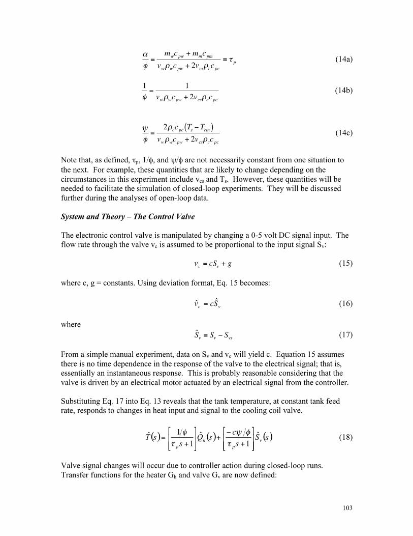
103

!

"

#=

mwcpw + mmcpm

vw$wcpw + 2vcs$cc pc% & p (14a)

!

1

"=

1

vw#wcpw + 2vcs#cc pc (14b)

!

"

#=

2$cc pc Ts %Tcin( )vw$wcpw + 2vcs$cc pc

(14c)

Note that, as defined, τp, 1/φ, and ψ/φ are not necessarily constant from one situation to the next. For example, these quantities that are likely to change depending on the circumstances in this experiment include vcs and Ts. However, these quantities will be needed to facilitate the simulation of closed-loop experiments. They will be discussed further during the analyses of open-loop data. System and Theory – The Control Valve The electronic control valve is manipulated by changing a 0-5 volt DC signal input. The flow rate through the valve vc is assumed to be proportional to the input signal Sv:

!

vc = cSv + g (15) where c, g = constants. Using deviation format, Eq. 15 becomes:

vcScv ˆˆ = (16)

where

!

ˆ S v" S

v# S

vs (17)

From a simple manual experiment, data on Sv and vc will yield c. Equation 15 assumes there is no time dependence in the response of the valve to the electrical signal; that is, essentially an instantaneous response. This is probably reasonable considering that the valve is driven by an electrical motor actuated by an electrical signal from the controller. Substituting Eq. 17 into Eq. 13 reveals that the tank temperature, at constant tank feed rate, responds to changes in heat input and signal to the cooling coil valve.

( ) ( ) ( )sSs

csQ

ssT v

p

h

p

ˆ

1

ˆ

1

1ˆ

!!"

#

$$%

&

+

'+

!!"

#

$$%

&

+=

(

)*

(

) (18)

Valve signal changes will occur due to controller action during closed-loop runs. Transfer functions for the heater Gh and valve Gv are now defined:

104

1

1

+!

sG

p

h"

# and 1+

!"

s

cG

p

v#

$% (19)

System and Theory – Heater Transfer Function Consider an open-loop experiment wherein the signal to the valve is kept constant ( 0ˆ =

vS ), and a positive step change a (in Watts – see Note below) is applied to the

heating rate: saQh =ˆ . The system response is provided from Eq. 18:

( ) ( )s

asG

s

a

ssT h

p

=!!"

#

$$%

&

+=

1

1ˆ

'

( (20)

Eq. 20 can be written in terms of partial fractions:

( )!!"

#

$$%

&

+'=

1

1ˆ

ss

asT

p

p

(

(

) (21)

Apply the inverse LaPlace transform to get the open-loop system response:

( ) ( )pte

atT

!

"

##= 1ˆ (22)

The curve-fit of experimental T̂ vs. t data according to Eq. 22 will yield τp and a/φ. Knowing the value of a, the value of 1/φ is obtained. Referring to Eqs. 14a and 14b, the values of vw and vcs are known – the subscript “s” refers to the condition before the change was applied. Therefore, using Eq. 14b, the value of 1/φ just obtained via curve fit can be verified. Using Eq. 14a and the τp obtained via curve fit, the lumped quantity

!

mwcpw + mmcpm can be estimated. With this lumped quantity in hand, τp can be estimated for any situation in which vw and vcs are known. Note: The heater output is set using the Variac, which is calibrated with an arbitrary linear 0-100% (0-120 volts AC in this experiment). The heater can be assumed to follow Ohm’s Law such that the power dissipated P (watts) is given by:

!

P = I2R =V

2R , where I

= current (amps), V = voltage to heater (volts ac), and R = heater resistance (ohms). The heater resistance is posted on the agitator motor control board. Therefore, the step change value a above can be easily estimated from the change in variac setting, together with the power equation.

105

System and Theory – Valve Transfer Function Consider an open-loop experiment wherein the heating rate is kept constant ( 0ˆ =hQ ), and a positive step change b (in volts dc) is applied to the signal to the coolant valve:

sbSv=ˆ . The system response is provided from Eq. 18:

( ) ( )s

bsG

s

b

s

csT v

p

=!!"

#

$$%

&

+

'=

1

ˆ

(

)* (23)

Eq. 23 can be written in terms of partial fractions :

( )!!"

#

$$%

&

+'

'=

1

1ˆ

ss

bcsT

p

p

(

(

)

* (24)

Apply the inverse LaPlace transform to get the open-loop system response:

( ) ( )pte

bctT

!

"

# $$

$= 1ˆ (25)

A curve-fit of experimental T̂ vs. t data according to Eq. 25 should yield τp and bcψ/φ. Knowing the values for b and c, the ratio ψ/φ is estimated. Fitting of open-loop experimental data using Eqs. 22 and 25 provides two estimates of τp. Eq. 14a shows that, τp might not be a constant due to the way it is defined. Assuming the same water level in the tank, and the same water rate through the tank (vw), τp will depend on the steady-state value of the coolant rate (vcs) prior to any change or event. In a similar way, ψ/φ will depend on vcs and Ts. Referring to Eqs. 14a and 14c, the values of vw, vcs, and Ts are known – the subscript “s” refers to the condition before the change was applied. Therefore, using Eq. 14c, the value of ψ/φ just obtained via curve fit can be verified. Using Eq. 14a and the τp obtained via curve fit, the lumped quantity

!

mwcpw + mmcpm can be estimated. With this lumped quantity in hand, τp can be estimated for any situation in which vw and vcs are known. The value of this lumped quantity obtained here should be consistent with the value obtained for it in the prior open-loop experiment. If they are not too different, a mean is recommended. System and Theory – Block Diagram A block diagram for the feedback-controlled system is shown in Figure 2. From block diagram algebra, it can easily be shown that:

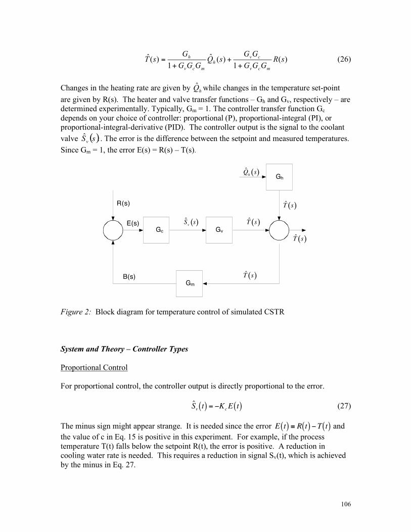
106

)(1

)(ˆ1

)(ˆ sRGGG

GGsQ

GGG

GsT

mcv

cv

h

mcv

h

++

+= (26)

Changes in the heating rate are given by hQ̂ while changes in the temperature set-point are given by R(s). The heater and valve transfer functions – Gh and Gv, respectively – are determined experimentally. Typically, Gm = 1. The controller transfer function Gc depends on your choice of controller: proportional (P), proportional-integral (PI), or proportional-integral-derivative (PID). The controller output is the signal to the coolant valve ( ).ˆ sS

v. The error is the difference between the setpoint and measured temperatures.

Since Gm = 1, the error E(s) = R(s) – T(s).

Gh

GvGc

R(s)

GmB(s)

E(s)

!

ˆ Q h

s( )

!

ˆ S v

s( )

!

ˆ T s( )

!

ˆ T s( )!

ˆ T s( )!

ˆ T s( )

Figure 2: Block diagram for temperature control of simulated CSTR System and Theory – Controller Types Proportional Control For proportional control, the controller output is directly proportional to the error.

!

ˆ S v

t( ) = "KcE t( ) (27)

The minus sign might appear strange. It is needed since the error

!

E t( ) " R t( ) #T t( ) and the value of c in Eq. 15 is positive in this experiment. For example, if the process temperature T(t) falls below the setpoint R(t), the error is positive. A reduction in cooling water rate is needed. This requires a reduction in signal Sv(t), which is achieved by the minus in Eq. 27.

107

In LaPlace form, the controller equation becomes:

!

ˆ S v

s( ) = GcE s( ) = "K

cE s( ) (28)

where Kc = the “gain”, while 100/gain is often called the “proportional band”. Proportional-Integral Control For proportional-integral control, the controller output also depends on the accumulated error. In this way, offsets can generally be eliminated.

!

ˆ S v

t( ) = "Kc

E t( ) +1

#i

E t( )dt

0

t

$%

& '

(

) * (29)

Applying LaPlace transforms, the controller equation becomes:

!

ˆ S v

s( ) = GcE s( ) = "K

c1+

1

#is

$

% &

'

( ) E s( ) (30)

where 1/τi is often called the “integral rate” or “reset”. Proportional-Integral-Derivative Control For proportional-integral-derivative control, the controller output also depends on the rate of change of the error. In this way, instabilities can be avoided.

!

ˆ S v

t( ) = "Kc

E t( ) +1

#i

E t( )dt + #d

dE t( )dt

0

t

$%

& '

(

) * (31)

Applying LaPlace transforms, the controller equation becomes:

!

ˆ S v

s( ) = GcE s( ) = "K

c1+

1

#is

+ #ds

$

% &

'

( ) E s( ) (32)

where τd is often called the “derivative time.” OUR STRATEGY: As seen from Eq. 26, there are two classes of experiments that can be performed : change in heating rate ( )sQh

ˆ (a disturbance), or a change in set point R(s). With three types of controllers, this suggests six possible experiments – far too many. In order to get the flavor of feedback control problems, two problems will be required: I) Change in set point under P control, and II) Disturbance under PI control. If time allows, you are free to choose a problem.

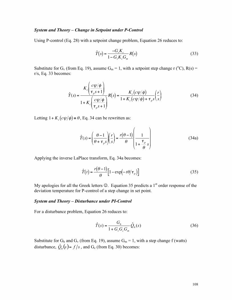
108

System and Theory – Change in Setpoint under P-Control Using P-control (Eq. 28) with a setpoint change problem, Equation 26 reduces to:

!

ˆ T s( ) ="G

vK

c

1"GvK

cG

m

R s( ) (33)

Substitute for Gv (from Eq. 19), assume Gm = 1, with a setpoint step change r (oC), R(s) = r/s, Eq. 33 becomes:

!

ˆ T (s) =

Kc

c" #

$ ps +1

%

& ' '

(

) * *

1+ Kc

c" #

$ ps +1

%

& ' '

(

) * *

R s( ) =Kc c" #( )

1+ Kc c" #( ) + $ ps

r

s

%

& ' (

) * (34)

Letting

!

1+ Kcc" #( ) $% , Eq. 34 can be rewritten as:

!

ˆ T (s) =" #1

" + $ ps

%

& ' '

(

) * *

r

s

%

& ' (

) * =

r " #1( )"

1

1+$ p

"s

%

&

' ' '

(

)

* * * (34a)

Applying the inverse LaPlace transform, Eq. 34a becomes:

!

ˆ T t( ) =r " #1( )"

1# exp # t" $ p( )[ ] (35)

My apologies for all the Greek letters . Equation 35 predicts a 1st order response of the deviation temperature for P-control of a step change in set point. System and Theory – Disturbance under PI-Control For a disturbance problem, Equation 26 reduces to:

)(ˆ1

)(ˆ sQGGG

GsT h

mcv

h

+= (36)

Substitute for Gh and Gv (from Eq. 19), assume Gm = 1, with a step change f (watts) disturbance, ( ) sfsQh =ˆ , and Gc (from Eq. 30) becomes:

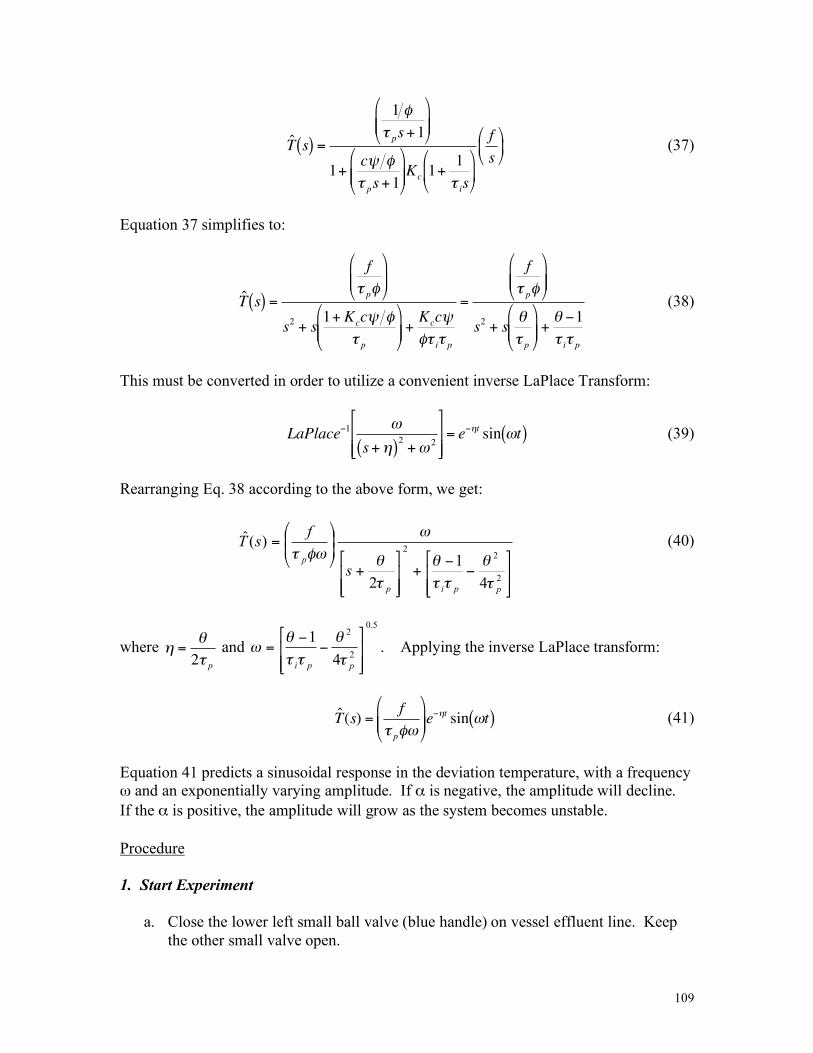
109

!

ˆ T s( ) =

1 "

# ps +1

$

% & &

'

( ) )

1+c* "

# ps +1

$

% & &

'

( ) ) Kc 1+

1

# is

$

% &

'

( )

f

s

$

% &

'

( ) (37)

Equation 37 simplifies to:

!

ˆ T s( ) =

f

" p#

$

% & &

'

( ) )

s2 + s

1+ Kcc* #

" p

$

% & &

'

( ) ) +

Kcc*

#" i" p

=

f

" p#

$

% & &

'

( ) )

s2 + s

+

" p

$

% & &

'

( ) ) +

+ ,1

" i" p

(38)

This must be converted in order to utilize a convenient inverse LaPlace Transform:

!

LaPlace"1 #

s+$( )2

+# 2

%

& ' '

(

) * *

= e"$t sin #t( ) (39)

Rearranging Eq. 38 according to the above form, we get:

!!"

#

$$%

&'

'+

!!"

#

$$%

&+

((

)

*

++

,

-=

2

22

4

1

2

)(ˆ

ppip

p

s

fsT

.

/

..

/

.

/

0

10. (40)

where

!

" =#

2$ p and

5.0

2

2

4

1

!!"

#

$$%

&'

'=

ppi (

)

((

)* . Applying the inverse LaPlace transform:

!

ˆ T (s) =f

" p#$

%

& ' '

(

) * * e

+,tsin $t( ) (41)

Equation 41 predicts a sinusoidal response in the deviation temperature, with a frequency ω and an exponentially varying amplitude. If α is negative, the amplitude will decline. If the α is positive, the amplitude will grow as the system becomes unstable. Procedure 1. Start Experiment

a. Close the lower left small ball valve (blue handle) on vessel effluent line. Keep the other small valve open.

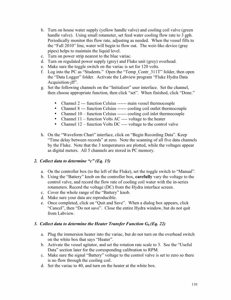
110

b. Turn on house water supply (yellow handle valve) and cooling coil valve (green handle valve). Using small rotameter, set feed water cooling flow rate to 3 gph. Periodically monitor this flow rate, adjusting as needed. When the vessel fills to the “Fall 2010” line, water will begin to flow out. The weir-like device (gray pipes) helps to maintain the liquid level.

c. Turn on power strip nearest to the blue variac. d. Turn on regulated power supply (grey) and Fluke unit (grey) overhead. e. Make sure the toggle switch on the variac is set for 120 volts. f. Log into the PC as “Students.” Open the “Temp_Contr_311T” folder, then open

the “Data Logger” folder. Activate the Labview program “Fluke Hydra Data Acquisition-jff”.

g. Set the following channels on the “Initializer” user interface. Set the channel, then choose appropriate function, then click “set”. When finished, click “Done.”

• Channel 2 --- function Celsius ------ main vessel thermocouple • Channel 8 --- function Celsius ------ cooling coil outlet thermocouple • Channel 10 – function Celsius ------ cooling coil inlet thermocouple • Channel 11 – function Volts AC ---- voltage to the heater • Channel 12 – function Volts DC ---- voltage to the control valve

h. On the “Waveform Chart” interface, click on “Begin Recording Data”. Keep “Time delay between records” at zero. Note the scanning of all five data channels by the Fluke. Note that the 3 temperatures are plotted, while the voltages appear as digital meters. All 5 channels are stored in PC memory.

2. Collect data to determine “c” (Eq. 15)

a. On the controller box (to the left of the Fluke), set the toggle switch to “Manual”. b. Using the “Battery” knob on the controller box, carefully vary the voltage to the

control valve, and record the flow rate of cooling coil water with the in-series rotameters. Record the voltage (DC) from the Hydra interface screen.

c. Cover the whole range of the “Battery” knob. d. Make sure your data are reproducible. e. Once completed, click on “Quit and Save”. When a dialog box appears, click

“Cancel”, then “Do not save”. Close the entire Hydra window, but do not quit from Labview.

3. Collect data to determine the Heater Transfer Function Gh (Eq. 22)

a. Plug the immersion heater into the variac, but do not turn on the overhead switch on the white box that says “Heater”.

b. Activate the vessel agitator, and set the rotation rate scale to 3. See the “Useful Data” section later for the corresponding calibration to RPM.

c. Make sure the signal “Battery” voltage to the control valve is set to zero so there is no flow through the cooling coil.

d. Set the variac to 40, and turn on the heater at the white box.

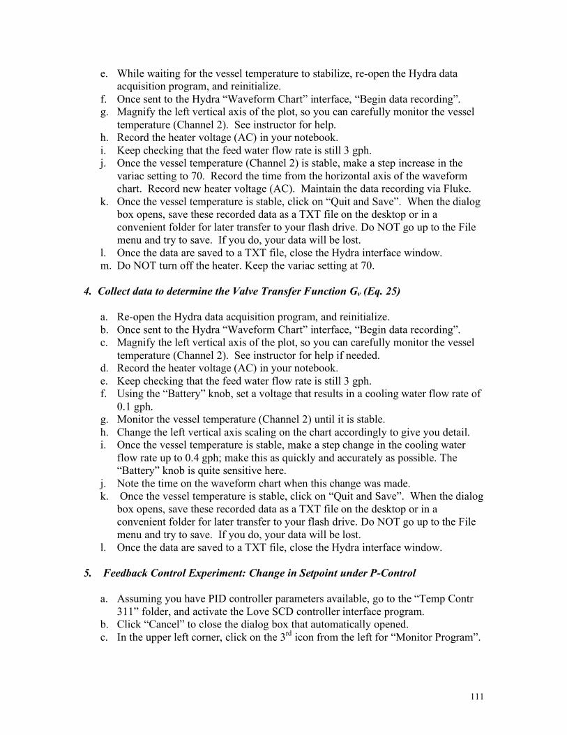
111

e. While waiting for the vessel temperature to stabilize, re-open the Hydra data acquisition program, and reinitialize.

f. Once sent to the Hydra “Waveform Chart” interface, “Begin data recording”. g. Magnify the left vertical axis of the plot, so you can carefully monitor the vessel

temperature (Channel 2). See instructor for help. h. Record the heater voltage (AC) in your notebook. i. Keep checking that the feed water flow rate is still 3 gph. j. Once the vessel temperature (Channel 2) is stable, make a step increase in the

variac setting to 70. Record the time from the horizontal axis of the waveform chart. Record new heater voltage (AC). Maintain the data recording via Fluke.

k. Once the vessel temperature is stable, click on “Quit and Save”. When the dialog box opens, save these recorded data as a TXT file on the desktop or in a convenient folder for later transfer to your flash drive. Do NOT go up to the File menu and try to save. If you do, your data will be lost.

l. Once the data are saved to a TXT file, close the Hydra interface window. m. Do NOT turn off the heater. Keep the variac setting at 70.

4. Collect data to determine the Valve Transfer Function Gv (Eq. 25)

a. Re-open the Hydra data acquisition program, and reinitialize. b. Once sent to the Hydra “Waveform Chart” interface, “Begin data recording”. c. Magnify the left vertical axis of the plot, so you can carefully monitor the vessel

temperature (Channel 2). See instructor for help if needed. d. Record the heater voltage (AC) in your notebook. e. Keep checking that the feed water flow rate is still 3 gph. f. Using the “Battery” knob, set a voltage that results in a cooling water flow rate of

0.1 gph. g. Monitor the vessel temperature (Channel 2) until it is stable. h. Change the left vertical axis scaling on the chart accordingly to give you detail. i. Once the vessel temperature is stable, make a step change in the cooling water

flow rate up to 0.4 gph; make this as quickly and accurately as possible. The “Battery” knob is quite sensitive here.

j. Note the time on the waveform chart when this change was made. k. Once the vessel temperature is stable, click on “Quit and Save”. When the dialog

box opens, save these recorded data as a TXT file on the desktop or in a convenient folder for later transfer to your flash drive. Do NOT go up to the File menu and try to save. If you do, your data will be lost.

l. Once the data are saved to a TXT file, close the Hydra interface window. 5. Feedback Control Experiment: Change in Setpoint under P-Control

a. Assuming you have PID controller parameters available, go to the “Temp Contr 311” folder, and activate the Love SCD controller interface program.

b. Click “Cancel” to close the dialog box that automatically opened. c. In the upper left corner, click on the 3rd icon from the left for “Monitor Program”.

112

d. In the first box of 4 that appear, clock on “Connect”. A user interface panel to the controller should appear.

e. Set the setpoint (SV) to 28 oC on the “Input” box of the Love window. In the “PID” box, set the proportional band (Pb) to the desired value (see instructor). Set all remaining parameters in that box to zero. Just enter the values, but don’t hit ‘return’. Use the tab key. After making your changes, go the “Parameters” on the upper left pulld-down menu, and click on “Upload” to send the changes to the controller. After uploading, click “OK” on the little dialog box that opens. Make sure your changes have been entered and remain.

f. Make sure the variac is set to 70, feed water rate to 3 gph, and cooling coil rate to 0.4 gph.

g. Re-activate the Hydra program, and begin data recording. Set scaling as needed. h. Activate the feedback control by flipping the controller box toggle switch to

“Auto”. Be careful that the switch has 3 positions. The middle position is null. Make sure the switch is all the way down.

i. Keep checking the feed water rate (0.3 gph) as it might have dropped once the cooling water flow began. They are coming from the same pipe.

j. Observe fluctuations in cooling water rate as controller achieves its stable value. Note that even if the cooling water rate falls to zero, there is a non-zero control signal voltage being sent to the valve. The valve simply is out of range here.

k. Once the vessel temperature is stable, go to the Love window, and change the setpoint to 30 oC. Upload the change using the “Parameter” menu. Note the time on the Hydra waveform chart. Maintain the data recording.

l. Once the vessel temperature is stable, “Quit and Save” your data from the Fluke. Close the Hydra window after saving your data as a TXT file.

7. Feedback Control Experiment: Disturbance under PI-Control

a. Reactivate the Hydra data collection program, and restart collecting data. b. Return to the Love controller interface, and change the Pb and Ti values to those

you have chosen for PI control (see instructor). Make sure you upload your changes.

c. Allow the system to stabilize. d. Once the vessel temperature is stable, increase the variac setting to 100. Let the

system respond and stabilize. Record the time and AC voltage from the Hydra interface window.

e. Once the vessel temperature is stable, “Quit and Save” your data as a TXT file. Close the Hydra window. Exit Labview.

8. Shutdown of Experiment and Data Retrieval

a. Turn off heater at the white box, then unplug the heater. b. Return the variac to zero, and turn off the agitator. c. Exit from the Love controller program. d. Turn off the Fluke and the power supply above it. e. Turn off the power strip next to the variac.

113

f. Turn off the water valves, and drain the vessel. g. Transfer all data files to a flash drive. Delete these files once you have confirmed

that the transfer is valid. You may also wish to email the files to your account. Data Analysis and Discussion • Be careful to use correct and consistent units during all the steps that follow. Verify

all the relevant derivations in the Theory section. • The Fluke Hydra data unit consumes real time in scanning over 5 input channels.

Therefore, a correction must be made. See the plot after References to on how to correct the “Labview time” to real (clock) time. All experimental time dependent data that you have collected should be corrected such that the recorded time is increased according to the calibration. See instructor if needed.

1. Estimation of c

a. Retrieve the coolant flow rate vc vs. signal to valve Sv data. b. Fit these data to a linear form according to Eq. 15. c. Estimate c from the slope.

2. Estimation of Heater Transfer Function Gh

a. Retrieve the vessel fluid temperature T vs. time t data for the no-coolant-flow open-loop experiment.

b. Convert the T(t) data to deviation format ( )tT̂ . c. Fit the experimental ( )tT̂ vs. t data according to Eq. 22, and obtain τp and a/φ.

Knowing a, determine 1/φ. d. Verify 1/φ using Eq. 14b and the values of vw and vcs at the time immediately

preceding the open-loop step change in heating rate. e. Using Eq. 14a and τp from the curve fit, obtain a value for the lumped quantity

!

mwcpw + mmcpm .

3. Estimation of the Valve Transfer Function Gv

a. Retrieve the vessel fluid temperature T vs. time t data for the constant heat input open-loop experiment.

b. Convert the T(t) data to deviation format ( )tT̂ . c. Fit the experimental ( )tT̂ vs. t data according to Eq. 25, and obtain τp and -bcψ/φ.

Knowing b and c, determine ψ/φ. d. Verify ψ/φ using Eq. 14c and the values of vw, vcs, and Ts at the time immediately

preceding the open-loop step change in voltage to the cooling valve. e. Using Eq. 14a and τp from the curve fit, obtain a value for the lumped quantity

!

mwcpw + mmcpm . Compare to the value obtained above. If not too dissimilar, take a mean quantity between the two values.

114

4. Modeling of the System Response under Proportional Control

a. Retrieve the height T(t) vs. time t data for the closed-loop (Proportional Gain only) experiment where you applied a step change disturbance to the setpoint.

b. Using your values for the constants and parameters in Eq. 35, predict the closed loop response for ( )tT̂ to the step increase in setpoint. Then be sure to calculate T(t) --- the absolute temperature. Be wary of all units! Within Eq. 35, for θ, get ψ/φ from Eq. 14c using the values of vw, vcs, and Ts in effect just before the step change in setpoint. Use τp as estimated using Eq. 14a, vw and vcs, and the mean value of the lumped quantity

!

mwcpw + mmcpm . c. On a single plot, compare the experimental T(t) to the predicted T(t). d. Comment on how well your model performs. What are some possible sources of

any deviations? 5. Modeling of the System Response under Proportional-Integral Control

a. Retrieve the height T(t) vs. time t data for the closed-loop (PI control) experiment where you applied a step change disturbance to the heating rate.

b. Using your values for the constants and parameters in Eq. 41, predict the closed loop response for ( )tT̂ to the step increase disturbance in heating rate. Then be sure to calculate T(t) --- the absolute temperature. Be wary of all units! Within Eq. 41, use τp as estimated using Eq. 14a, vw and vcs, and the mean value of the lumped quantity

!

mwcpw + mmcpm . Similarly, obtain 1/φ from Eq. 14b. For η and ω, obtain θ using ψ/φ from Eq. 14c with the values of vw, vcs, and Ts in effect just before the step change in heating rate.

c. On a single plot, compare the experimental T(t) to the predicted T(t). d. Comment on how well your model performs. What are some possible sources of

any deviations? 6. Items to Consider in the Conclusion Comment on the models to predict observed closed loop behavior. Were the models adequate? If not, what is the likely most important problem? Is the model incorrect? Is the key assumption regarding the valve not valid? The assumption

!

UoAo >> 2vc"cc pc was used in Eq. 8. Was this a valid assumption? Use standard techniques to estimate Uo (see Batch Heat Transfer in ChE 396 Manual). The calibration for the agitator speed References 1. Harriot, P., “Process Control”, McGraw-Hill Book Co., New York, N.Y. (1964).

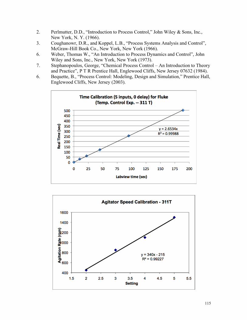
115

2. Perlmutter, D.D., “Introduction to Process Control,” John Wiley & Sons, Inc., New York, N. Y. (1966).

3. Coughanowr, D.R., and Koppel, L.B., “Process Systems Analysis and Control”, McGraw-Hill Book Co., New York, New York (1966).

6. Weber, Thomas W., “An Introduction to Process Dynamics and Control”, John Wiley and Sons, Inc., New York, New York (1973).

7. Stephanopoulos, George, “Chemical Process Control – An Introduction to Theory and Practice”, P T R Prentice Hall, Englewood Cliffs, New Jersey 07632 (1984).

6. Bequette, B., “Process Control: Modeling, Design and Simulation,” Prentice Hall, Englewood Cliffs, New Jersey (2003).

116

Protein Oxidation (311 T) Introduction In this experiment, liquid egg whites are reacted with household bleach in a flow reactor. Raw (i.e. in the chicken egg) egg whites are approximately 12 weight % proteins with a balance of water. The largest component protein in egg whites is ovalbumin, with a molecular weight of 45 kiloDaltons (kDa), also known as 45,000 amu. The powdered (i.e. dehydrated) egg whites to be used as essentially all protein. The solution to be used will be 10% (by weight) of powdered egg whites, with a balance of water. Since the molecular weight of the protein is so large, the molar concentration will be quite small. The active ingredient in household bleach is 6 weight % NaOCl with a balance of water and other inerts. The NaOCl oxidizes the proteins, and heat is released. Practical volumetric flow rates (~ 1 gph or more for each solution) will be used in this experiment. The result will be a great excess of NaOCl compared to the protein on a molar basis. Objectives The objectives include the investigation of a complex reaction system for which the stoichiometry and kinetics are ill defined. The analysis will depend largely on temperature data. Considerable assumptions will be made. This method is contrary to the stated, preferred approach in this course of trying to use literature-based, design modeling to try to predict our observations. Reaction Kinetics Let A ≡ protein, and B ≡ NaOCl. The reaction will be taken to be:

A + nB products (1) where the coefficient n is not known. Assume a simple kinetic rate expression:

!

"rA = # k CACB = Af exp "EA

RT

$

% &

'

( ) CACB (2)

In this experiment,

!

CB" C

Bo>>C

A. Species A will be the key for our modeling.

Reactor Species Balance

Assume a plug flow reactor model. This is gross simplification since typical Reynolds numbers in this experiment will indicate laminar flow. However, a laminar flow analysis will seriously complicate the problem. The plug flow species A balance is given by:

117

!

rA

=dF

A

dV= v

o

dCA

dV (3)

where

!

FA

= CAvo. Equation (2) becomes:

!

"rA # AfCBo exp "EA

RT

$

% &

'

( ) CA (4)

Reactor Energy Balance The reaction to be studied is exothermic, though only a modest temperature rise is expected. Even though the reactor is mostly glass – a good insulator – heat losses should be considered. A plug flow reactor energy balance is assumed:

!

dT

dV="rA( ) "#HrA( ) "Ua T "Tr( )

voc p$ (5)

The heat of reaction and mean physical properties are taken to be constant. The set of Equations (3), (4), and (5) are to be solved simultaneously between the reactor inlet and outlet. However, the thermo-kinetic parameters (Af, ΔHrA, EA) are not known, and must be guessed. Some guidance exists for ΔHrA. The heat of combustion of protein is ~ 5 kcal/gram. This suggests ΔHrA ~ 4 kcal/gram. The other parameters (CBo,

!

c p ,

!

" , vo, CAo) are known or can be estimated. It is recommended that mass units be used for the concentrations. The goal is to find the parameters that result in a decent match to the observed temperatures. Reactor Heat Loss Calibration Consider Eq. (5) without the reaction:

!

dT

dV="Ua T "Tr( )

voc p# (6)

A simple integration yields:

!

lnT "Tr

To "Tr

#

$ %

&

' ( =

"UaV

c p)

#

$ % %

&

' ( ( 1

vo

(7)

A plot of outlet temperature T vs. total volumetric flow rate vo according to Eq. (7) should yield a slope containing the Ua heat loss factor for use in the reactive simulation. If not linear, then Ua might be a function of flow rate – consult the instructor.

118

Procedure Heat Loss Calibration Note: Prior to starting this task, consult with the instructor. 1. Make sure the overhead feed egg white solution container is clean. 2. Locate the extension hose at the house hot water source, and run it into the nearest

sink. Carefully open the hot water valves, and run water into the sink till the water is as warm as you feel it will get – probably about 15 minutes.

3. Once the water is fairly warm, turn off the flow. Carefully stretch the hose over to the Protein Oxidation experiment. Run the hose over the tables.

4. Carefully, fill egg white solution feed solution container with warm water. Carefully coil up the hose and return it.

5. Activate the data collection program on the PC. 6. Begin warm water flow through the reactor using the egg white plumbing. 7. Once the inlet and outlet temperatures are steady, change the warm water flow rate.

Continue the temperature trace for a series of flow rates across the available range of the flow meter. Take at least 4-5 different flow rates. Keep track on the trace (by noting elapsed time) when the flow rate is changed.

8. When finished, empty the egg white solution container of any water prior to filling with egg white solution.

9. Make sure to record room temperature via the analog dial thermometer provided. Preparation of Egg Whites Solution

1. Working on the adjacent bench, prepare ~ 6 gallons of 8-10% (by weight) powdered egg whites in aqueous solution.

2. Use Honeyville Farms egg white powder, together with room temperature tap water. Use a stirring plate but avoid warming.

3. Prepare the solution in batches of ~ 2 liters at a time. 4. Use sufficient agitation to dissolve the powder. Note that some foaming will

occur, though try not over-foam. 5. Pour the solution into the large plastic jug that is on the shelf over the experiment.

Fill the jug on the bench with a funnel, and then carefully lift the jug up onto the shelf. Reconnect the tubing. Ask the instructor for help if needed.

Bleach Solution

1. Make sure the bleach supply jug up on the overhead shelf is filled with 6 gallons of Clorox bleach or equivalent. Confirm with the TA or the instructor.

2. If not, carefully pour 6 gallons of bleach into the jug. Use a funnel. Observe the markings on the side of the jug.

119

Data Acquisition System

There are thermocouple and solution conductivity probes at both ends of the reactor. The signals from each are transferred to a PC running Vernier data collection software. NOTE: It is expected that there will be little conductivity change across the reactor since the NaOCl will be in excess. However, record all data available, and comment in your discussion as to whether the conductivity is indeed fairly constant. If not, consider why.

1. If not already activated, turn on the interfaces connecting the conductivity probes and thermocouples to the PC.

2. Inside the “My Documents” folder, open the “Protein Oxidation” folder. Activate the data collection program entitled “Laminar Reactor 2010.gmbl”. Upon opening, the PC should be ready to collect and plot live conductivity and temperature data.

3. Under the pull-down menu “Experimental”, verify the data collection rate at 1 record every 5 seconds. Set the data collection for “continuous” data collection. The run can be terminated earlier at will.

Reactor Operation The system is complicated with considerable plumbing. Review the system completely, and make sure you know what each valve does before starting.

1. Uncoil the long drain hose, and carefully lay it on the floor with outlet at drain. 2. Turn on the house water supply over on the far wall to the left of the sink.

Coordinate with the “Temperature Control” experiment group if necessary. 3. Direct water flow to the reactor, and rinse out the tube for at least 5 minutes. 4. Set egg white solution flow for recycle back to the feed tank, not the reactor.

Turn on the pump, and set the desired flow rate on the flowmeter. 5. Repeat step 5 for the bleach flow. Set the bleach flowrate to be twice the egg

white solution flow rate. Keep this ratio for all runs. 6. Begin data recording on the PC. 7. Turn off the water flow to the reactor. Begin water flow to the top of the gray,

vertical reactor effluent pipe. This will help to keep the drain hose rinsed. 8. Direct the egg white solution flow to the reactor, and wait for steady signals. 9. Direct the bleach to the reactor. Adjust both flow rates to the desired values. Note

the elapsed time. 10. Once signals are steady, vary both flow rates while keeping the same flow rate

ratio. Note the elapsed time. 11. Try to achieve as many flow rate pairs (i.e. total flow rates) as possible as long as

the bleach and egg white supply tanks have solution. If running low, consult with the instructor. Avoid letting the solutions run out and air enter the feed lines.

System Shutdown and Data Retrieval

1. Turn off both pumps, and set valves for reactant flows to be recycled to the tanks.

120

2. Turn off the water flow to the gray effluent pipe, and redirect water flow to the reactor for at least 10 minutes of washout.

3. While washing out, save the Vernier data file. Also, copy the columns of data into a separate spreadsheet as a backup.

4. Shut down main water source at the far wall, and turn off all valves in the system. 5. Carefully assist the TA in draining out the effluent hose without making a huge

mess on the floor. Coil the empty hose around the distilled water jug at the end of the bench.

Data Analysis, Modeling, and Discussion

1. Regression the “heat loss” temperature data according to Equation (7). 2. Solve the set of Equations (4), (5), and (3) simultaneously between the reactor

inlet and outlet for each run. 3. The estimated parameters should be reasonable. Use care with units! For each

run, vary the estimates until the outlet temperature is close to what was observed experimentally. NOTE: There are a few guidelines that might help:

a. Af and EA > 0; ΔHrA < 0; CA > 0 b. An upper limit on ΔHrA is the heat of combustion of protein (~ 5 kcal/g);

suggest ΔHrA ~ 4 kcal/gram protein.

4. Discuss the observed variation in values for Af and EA. Are the values at all consistent and reasonable? Consider that all three parameters should be constants. Try to choose an “optimal” set of values, and rerun the simulations with this set.

5. Consider reasons for any serious discrepancies. 6. How sure are you of your model? How sure are you of your data? 7. How good is the assumption of a plug flow reactor? Estimate the Reynolds

numbers for your runs. What do you conclude? Nomenclature

T = reactor temperature (K) CB, CA = molar concentrations of NaOCl, protein (moles/liter) FA = molar flow rate of protein in the reactor (moles/min)

!

c p = mean heat capacity of reactor liquid (cal/gram-K) – assume value for water

!

" = mean mass density of reactor liquid (gram/liter) – assume specific gravity of 1.1 k = second order reaction rate constant (liter/mole-min) Af = Arrhenius pre-exponential factor for rate constant (liter/mole-min) EA = Arrhenius activation energy (cal/mole) R = ideal gas constant (1.987 cal/mole-K) rA = rate of reaction based on protein (mole/liter-min) V = reactor volume (liters) vo = volumetric flow rate (liters/min) ΔHrA = heat of reaction per mole of A (cal/mole)

121

To = feed temperature to the reactor (K) CAo = feed concentration of protein to the reactor (mole/liter) U = overall heat transfer coefficient (cal/min-cm2-K) a = heat transfer area / unit reactor volume (cm2/liter) Tr = room temperature (K) References Fogler, H. S., Elements of Chemical Reaction Engineering, 4th ed., Prentice-Hall, NJ (2006). Baker, R. W. R., “Studies on the Reaction between Sodium Hypochlorite and Proteins,” Biochemistry, vol. 41, pp. 337-342 (1947). Paladines, O. L., et al., “Heat of Combustion of the Protein and Fat in the Body and Wool of Sheep,” Journal of Nutrition, vol. 82, no. 1, p. 145+ (1964).