R E S E A R CH A R T I C L E

Charting shared developmental trajectories ofcortical thickness and structural connectivityin childhood and adolescence

Gareth Ball1 | Richard Beare1 | Marc L. Seal1,2

1Developmental Imaging, Murdoch Children's

Research Institute, Melbourne, Victoria,

Australia

2Department of Paediatrics, University of

Melbourne, Melbourne, Victoria, Australia

Correspondence

Gareth Ball, Developmental Imaging, Murdoch

Children's Research Institute, Melbourne,

Victoria, Australia.

Email: gareth.ball@mcri.edu.au

Funding information

National Institute of Mental Health; State

Government of Victoria; University of

Melbourne; Royal Children's Hospital;

Murdoch Childrens Research Institute

Abstract

The cortex is organised into broadly hierarchical functional systems with distinct

neuroanatomical characteristics reflected by macroscopic measures of cortical mor-

phology. Diffusion-weighted magnetic resonance imaging allows the delineation of

areal connectivity, changes to which reflect the ongoing maturation of white matter

tracts. These developmental processes are intrinsically linked with timing coincident

with the development of cognitive function. In this study, we use a data-driven multi-

variate approach, nonnegative matrix factorisation, to define cortical regions that co-

vary together across a large paediatric cohort (n = 456) and are associated with spe-

cific subnetworks of cortical connectivity. We find that age between 3 and 21 years

is associated with accelerated cortical thinning in frontoparietal regions, whereas rel-

ative thinning of primary motor and sensory regions is slower. Together, the subject-

specific weights of the derived set of cortical components can be combined to pre-

dict chronological age. Structural connectivity networks reveal a relative increase in

strength in connection within, as opposed to between hemispheres that vary in line

with cortical changes. We confirm our findings in an independent sample.

K E YWORD S

brain development, connectivity, cortex, diffusion MRI, magnetic resonance imaging, matrix

factorisation, multivariate

1 | INTRODUCTION

Brain development during childhood and adolescence has been

well-characterised in recent years using magnetic resonance imaging

(MRI) (Mills et al., 2016). MRI provides a noninvasive method to examine

neuroanatomy at a multiple scales. Analyses of structural MRI have

found that the volume of grey and white matter follows different

developmental trajectories during childhood.

Longitudinal analyses describe widespread and regionally variable

decreases in cortical volume and thickness over childhood, with the

largest decreases in thickness observed in the parietal lobe and the

smallest changes in primary sensory-motor cortex (Tamnes et al.,

2017; Vijayakumar et al., 2016; Wierenga, Langen, Oranje, & Durston,

2014). During childhood, observable patterns of cortical thinning, in

part, reflect changes to the tissue microstructure (Huttenlocher, 1979;

Pakkenberg & Gundersen, 1997; Vértes & Bullmore, 2015). Over the

same period, significant maturation of the brain's white matter occurs,

with increases in overall volume and continuing axonal myelination

(Lebel & Beaulieu, 2011; Lebel & Deoni, 2018; Tamnes et al., 2010).

The cortex is organised into broadly hierarchical functional systems

with distinct neuroanatomical characteristics, including neuronal den-

sity and cortico-cortical connectivity (Collins, Airey, Young, Leitch, &

Kaas, 2010; Felleman & Van Essen, 1991; Markov et al., 2013). Areal

differences in cortical cytoarchitecture mirror this hierarchy (Collins

et al., 2010), a pattern that is reflected by macroscopic measures of cor-

tical morphology (Wagstyl, Ronan, Goodyer, & Fletcher, 2015). At a

Received: 9 March 2019 Revised: 5 June 2019 Accepted: 5 July 2019

DOI: 10.1002/hbm.24726

4630 © 2019 Wiley Periodicals, Inc. Hum Brain Mapp. 2019;40:4630–4644.wileyonlinelibrary.com/journal/hbm

microscopic level, neuronal density is inversely related to cortical thick-

ness (Cahalane, Charvet, & Finlay, 2012; Schüz & Palm, 1989; Wagstyl

et al., 2015), whereas synaptic density tends to increase with increasing

thickness (Schüz & Palm, 1989).

Diffusion-weighted MRI allows the delineation of macroscale areal

connectivity, changes to which reflect the ongoing maturation of white

matter tracts. These developmental changes vary in timing and extent

in a regional pattern that likely reflects the functional organisation of

the brain. Studies using diffusion MRI have shown markers of tissue

organisation, including fractional anisotropy (FA), increase with age dur-

ing childhood (Lebel, Walker, Leemans, Phillips, & Beaulieu, 2008), with

maturation of commissural and projection fibres regions preceding

intrahemispheric association fibres (Lebel & Beaulieu, 2011). The

effects of white matter maturation on structural connectivity measures

reveal large-scale topological organisation of the structural connectome

with measures of network efficiency and modularity increasing over

childhood and adolescence (Baum et al., 2017; Zhao et al., 2015).

It is likely these developmental processes are intrinsically linked

(Van Essen, 1997; Herculano-Houzel, Mota, Wong, & Kaas, 2010;

Mota & Herculano-Houzel, 2012) with timing coincident with the

development of cognitive function (Blakemore & Choudhury, 2006).

In children, evidence of increased cortical thinning and white matter

maturation from MRI is associated with improved cognitive perfor-

mance (Kharitonova, Martin, Gabrieli, & Sheridan, 2013; Krogsrud

et al., 2018; Squeglia, Jacobus, Sorg, Jernigan, & Tapert, 2013).

Regional variation in both grey and white matter development

reflects the functional organisation of the brain, with lower order motor

and sensory regions developing before areas that support complex, exec-

utive function. In a recent study, Sotiras et al. used a data-driven,

multivariate method for dimension reduction, nonnegative matrix

factorisation (NMF), to identify a set of regional patterns of coordinated

decreases in cortical thickness during adolescence (Sotiras et al., 2017).

They found that changes in cortical thickness were spatially heteroge-

neous, with regional variation mirroring functional organisation and

genetic patterning (Sotiras et al., 2017). This modular organisation is

supported by evidence that cortical regions can be defined based on the

extent of their shared anatomical connections (Bullmore & Sporns, 2012;

Hilgetag, Burns, O'Neill, Scannell, & Young, 2000). Both neuronal density

and dendritic spine density are correlated to areal connectivity (Beul &

Hilgetag, 2019; Scholtens, Schmidt, de Reus, & van den MP, 2014),

and white matter networks derived from MRI can similarly be split in

subnetworks of connections, or modules, that appear to support known

cortical systems, vary together with age and can be disrupted in neu-

rodevelopmental disorder (Ball, Beare, & Seal, 2017; Baum et al., 2017;

Faskowitz, Yan, Zuo, & Sporns, 2018). Therefore, macroscopic markers

of brain development, including cortical thickness and measures of white

matter connectivity reflect regionally-varying patterns of complex, inter-

linked microscopic processes across the white and grey matter.

Multivariate methods, including NMF, are well-suited to neuroim-

aging analysis, enabling pattern discovery in large, complex data sets

(Ball, Beare, & Seal, 2017; Beckmann & Smith, 2005; Calhoun, Liu, &

Adalı, 2009; Sotiras, Resnick, & Davatzikos, 2015). Recently, a number

of multivariate methods have been described that aim to integrate

measures from different imaging modalities (Groves, Beckmann,

Smith, & Woolrich, 2011; Sui, Adali, Yu, & Calhoun, 2012). This allows

correlated patterns to be identified across imaging types, providing mul-

tiple views of developmental processes across tissue compartments.

NMF is particularly apt for MRI analysis given that most MR-derived

anatomical measures are nonnegative (cortical thickness, tissue volume,

FA, etc.) (Sotiras et al., 2015). When applied to anatomical data, NMF

returns sparse components that represent local patterns, or compo-

nents, of covariation that permit interpretation as regions of coordi-

nated growth or maturation (Sotiras et al., 2015, 2017). We have

previously applied this method to structural network data, revealing

subnetworks or network components, with connections that vary

together across subjects (Ball, Beare, & Seal, 2017).

In this article, we aim to combine these approaches to describe

how patterns of regional change in cortical thickness are associated

with specific patterns of change to structural connectivity networks

during childhood and adolescence. In a large development cohort, we

demonstrate that NMF provides hierarchical decomposition of the

cortex based on regional differences in cortical thickness change over

time. Additionally, using a supervised NMF approach, we define spe-

cific patterns of structural connectivity that vary over the population

in line with each cortical pattern.

2 | METHODS

2.1 | Data

Data were acquired from the PING Study (Jernigan et al., 2016). The

PING cohort comprises a large, typically-developing paediatric popula-

tion with participants from several U.S. sites included across a wide

age and socioeconomic range. The human research protections pro-

grams and institutional review boards at all institutions participating in

the PING study approved all experimental and consenting procedures,

and all methods were performed in accordance with the relevant

guidelines, regulations and PING data use agreement (Brown et al.,

2012). Written informed consent was obtained for all PING partici-

pants. Exclusion criteria included: (a) neurological disorders; (b) history

of head trauma; (c) preterm birth (less than 36 weeks); (d) diagnosis of

an autism spectrum disorder, bipolar disorder, schizophrenia, or mental

retardation; (e) pregnancy; and (f) daily illicit drug use by the mother for

more than one trimester (Jernigan et al., 2016). Similar proportions of

males and females participated across the entire age range.

The PING cohort included 1,493 participants aged 3 to 21 years,

of whom 1,249 also had neuroimaging data. Of these, n = 763 imaging

data sets were available to download.

2.2 | Neuroimaging

At each site, pulse sequences were optimised for equivalence in con-

trast properties across scanner manufacturers and models (Brown

et al., 2012; Jernigan et al., 2016). T1-weighted images were acquired

using standardised 3-Tesla high-resolution 3D RF-spoiled gradient

echo sequences with prospective motion correction (PROMO). Image

BALL ET AL. 4631

resolution was 1 × 1 × 1.2 mm (Siemens) or 0.9375 × 0.9375 × 1.2 mm

(GE). Diffusion data were acquired using axial 2D EPI scans with

30-directions, b-value = 1,000, resolution 2.5 × 2.5 mm (Siemens) or

1.875 × 1.875 (GE) and slice thickness = 2.5 mm with a corresponding

reverse-encoded b = 0 map for EPI B0-distortion correction. Detailed

acquisition parameters for each scanner manufacturer can be viewed

at: http://pingstudy.ucsd.edu/resources/neuroimaging-cores.html.

Quality control for the PING data is detailed in Jernigan et al.

(2016). In brief, images were inspected for excessive distortion,

operator compliance or scanner malfunction. We performed addi-

tional, on-site, visual quality control assessment of T1 and diffu-

sion data. This involved a visual inspection of T1 volumes for

motion or image acquisition or reconstruction artefacts. In addi-

tion, we included only diffusion data with at least one complete

30-direction acquisition, after inspection for slice-dropouts or

motion artefacts. Five participants were removed due to excessive

motion in T1-weighted images; a further 312 were removed due to

a lack of matched 30-direction sequences (n = 232), or due to

motion or image artefacts (n = 80).

This resulted in a final cohort of n = 456 participants with both

T1-weighted and 30-direction diffusion data from five scan sites (mean

age + S.D [range] = 12.6 + 4.91 [3.2–21.0] y, 233 male [51.1%]).

Site/scanner-specific demographic data are shown in Table S1.

2.3 | Discovery and validation cohorts

The full cohort was split into discovery and validation cohorts prior to

analysis. A random subset of 152 subjects (33%) were removed and

retained as a held-out validation cohort.

2.4 | Image processing

T1 MRI data were processed as in Ball Adamson, Beare, & Seal, (2017).

Briefly, vertex-wise maps of cortical thickness were constructed with

FreeSurfer 5.3 (http://surfer.nmr.mgh.harvard.edu). This process

includes removal of non-brain tissue, transformation to Talairach space,

intensity normalisation, tissue segmentation, and tessellation of the

grey matter/white matter boundary followed by automated topology

correction. Cortical geometry was matched across individual surfaces

using spherical registration (Dale, Fischl, & Sereno, 1999; Fischl et al.,

2002; Fischl & Dale, 2000; Fischl, Sereno, & Dale, 1999). Any images

that failed initial surface reconstruction, or returned surfaces with topo-

logical errors, were manually fixed and resubmitted to FreeSurfer until

all data sets completed reconstruction. To reduce computational load,

data were downsampled to the fsaverage5 surface comprising 10,242

vertices per hemisphere and smoothed to 10 mm FWHM.

Diffusion data were preprocessed using MRtrix 3.0 (http://www.

mrtrix.org/). Data were first denoised and corrected for EPI distor-

tions using topup/eddy (Andersson & Sotiropoulos, 2016; Veraart,

Fieremans, & Novikov, 2016). The diffusion signal at each voxel was

then modelled using a tensor model, from which we calculated FA

(Basser & Pierpaoli, 1996).

2.5 | Whole-brain tractography

Prior to tractography, each T1 image was segmented into three tissue

classes (grey matter, white matter, and cerebrospinal fluid) using FSL's

FAST (Zhang, Brady, & Smith, 2001) and the cortical grey matter

parcellated into n = 220 cortical regions-of-interest derived from sub-

divisisions of the Desikan-Killiany anatomical atlas using easy_lausanne

(https://github.com/mattcieslak/easy_lausanne) (Daducci et al., 2012;

Hagmann et al., 2008). Tissue segmentations and parcellations were

transformed into diffusion space using Boundary-Based Registration

(Greve & Fischl, 2009) followed by nonlinear registration using ANTS

(Avants, Epstein, Grossman, & Gee, 2008).

Probabilistic whole-brain fibre-tracking was performed using wild

bootstrap diffusion tensor tractography (Jones, 2008) implemented in

MRtrix3. Ten million streamlines were generated per participant with

a step size of 1 mm. Streamlines were seeded from the grey/white

matter interface and anatomically constrained using a 5-tissue-type

(5TT) mask (Smith, Tournier, Calamante, & Connelly, 2012).

Structural connectivity matrices (of size 220 × 220) were constructed

by identifying streamlines that connected cortical regions-of-interest

using a 2-mm radial search from streamline endpoints. For each pair

of connected regions, connection strength was estimated by calcu-

lating mean FA along all connecting streamlines.

After discounting connections that were zero across all subjects,

connectivity matrices were subject to a consistency-based thresholding,

retaining the top 10% most consistent edges across subjects and

resulting in n = 1,538 edges in the final set of networks (Roberts, Perry,

Roberts, Mitchell, & Breakspear, 2017).

2.6 | Site correction

To correct for possible effects of acquisition site on the initial NMF

decomposition, we used ComBat harmonisation (https://github.com/

ncullen93/neuroCombat) to estimate and remove linear site effects

from vertexwise measures of cortical thickness (see also Figure S3).

This method has been shown to remove unwanted sources of scan

variability in multisite analyses of cortical morphometry measures

(Fortin et al., 2018). We did not apply this method to the connectivity

data. Instead, due to the removal of site variation from the H matrix

(see below), we only consider edges that vary with each cortical com-

ponent, and therefore do not vary with site.

2.7 | Projective NMF

We decomposed cortical thickness data into a set of nonnegative,

orthogonal components using projective NMF (Ball, Beare, & Seal,

2017; Sotiras et al., 2015, 2017; Yang & Oja, 2010).

Briefly, NMF is a multivariate method that models an n feature × m

sample data matrix, V, as the product of two nonnegative matrices:

W with dimensions n × r and H with dimensions r × m, such that

V ≈ WH. Generally, the number of basis components r < min(m, n),

thus WH represents a low-rank approximation of the original data in V

(Lee & Seung, 1999).

4632 BALL ET AL.

In projective NMF, the matrix, H is replaced with WTV such that

V ≈ WWTV. PNMF confers a number of benefits over standard NMF

including fewer learned parameters and increased sparsity of the

resulting matrix W (Yang & Oja, 2010).

In this context, the columns of W represent a set of components,

each comprising cortical regions that covary together across the study

population and WTV provides a corresponding set of subject-specific

weights, one per component (Sotiras et al., 2015). Together, these

elements can be combined to approximately reconstruct any subject's

original data set.

We implemented PNMF in Python (3.6.3), performing 20,000 iter-

ations each time. Before NMF, each subject's cortical data were

normalised to unit norm as an equivalent operation to correcting each

vertex for mean cortical thickness, while ensuring nonnegativity.

2.8 | Supervised NMF

To identify structural connections that covary with each of the corti-

cal components, we performed a supervised NMF decomposition of

the structural connectivity data. We derive the subject loadings from

the PNMF decomposition of the cortical data: H=WTcorticalV and

decompose the connectivity data, Vconn by iteratively updating Wconn

to minimise the (Euclidean) distance between the original and

reconstructed matrices, subject to nonnegativity constraints, while

ensuring H remains fixed:

minW ≥0,H≥0

F =12

Xij

Vij− WHð Þijh i2

This results in a set of orthogonal network components, each

comprising a sparse set of (topologically) localised connections (i.e., :

the edge structure of different components does not overlap) and

each varying across the population in line with a given cortical compo-

nent. As with the cortical data, each subject's connectivity was

normalised prior to NMF.

2.9 | Reconstruction error, cross-validation, and ageprediction

For each set of components, we calculated the root mean square error

(RMSE) between the original data matrices and matrices reconstructed

from the NMF components for both cortical thickness and structural

connectivity. To reduce bias in our error estimation, we employedWold

holdouts (Wold, 1978), masking a random subset of 20% of elements

from each data matrix during NMF estimation and calculating error

within the held-out subset. Holdouts were repeated five times and

reconstruction error averaged across repeats.

In addition, to demonstrate the low-rank data representations

retains relevant neurobiological signal, we used each set of compo-

nent timecourses to predict chronological age. We used Gaussian pro-

cess regression implemented in scikit-learn (v0.20.0) to estimate age

for each subject based on their individual component weights within a

10-fold cross-validation framework (Cole et al., 2017). For each set of

components, age prediction error was calculated as the mean absolute

difference between predicted and chronological age.

2.10 | Modelling component timecourses

For each component, we used generalised additive models (GAMs) to

model the relationship between age and component weight using the

mgcv package in Rv3.5.1 (Wood, 2017). GAMs are flexible models that

allow a data-driven estimation of (possibly nonlinear) relationships

between variables. Component weight was modelled as a smooth

function of age, estimated using penalised thin plate regression splines

with automatic smoothness estimation maximising marginal likelihood

(ML) (Wood, 2003, 2011). For each component, we additionally tested

the inclusion of main effects of sex and site alongside age and com-

pared model fit using the Akaike information criterion (AIC).

2.11 | Network component analysis

To test whether network components comprised edge sets that were

significantly enriched for connection involving regions within the

corresponding cortical components, we modelled each component's

edge count using a hypergeometric distribution. We calculated the

probability that the observed proportion of edges connecting within

(or between) cortical components was drawn as a random sample

from the full (thresholded) network:

p= 1−Xx

i=0

Ki

� �M−KN− i

� �MN

� �

where p is the upper cumulative probability of finding x or more edges

connecting at least one region within a given cortical module drawn

randomly without replacement from a set of edges of size N, given

the overall number of edges connecting at least one region within a

given cortical module, K, and the size of the complete set of edges in

the thresholded network,M.

For all components, we calculated both the enrichment ratio

(i.e., : the proportion of network component edges connected to a

given cortical component divided by the proportion in the whole

network) and the hypergeometric probability, p, for edges

connecting at least one region within a given module. We corrected p-

values using false discovery rate (FDR) to account for multiple

comparisons.

2.12 | Hierarchical decomposition

Hierarchical clustering was performed using Ward's linkage based

on Euclidean distance between the component timecourses. The

cophenetic correlation was calculated between pairwise similarity and

dendrogram distance of component timecourses as a measure of hier-

archical organisation. Statistical significance was determined using

random permutations (p < .05, n = 10,000).

BALL ET AL. 4633

2.13 | Neurocognitive data

In addition to imaging data, participants in the PING study undertook

comprehensive behavioural and cognitive assessments (NIH Toolbox

Cognition Battery, NTCB). The NTCB comprises a set of tests that

measure abilities across several cognitive domains, including cognitive

flexibility, inhibitory control, and working memory, resulting in eight

measures of cognitive performance (for full details of these measures

in the PING cohort refer to Akshoomoff et al., 2014). In total, n = 253

(83%) in the discovery cohort and n = 124 (82%) had both imaging

and neurocognitive data.

To test associations between individual component weights

and cognitive performance, we first modelled each cognitive score

as a smooth function of age with an additional main effect of sex

using a GAM (Akshoomoff et al., 2014). For each scale, the resid-

uals of this model represent individual performance at a level

greater or lesser than expected for a given age and sex. Similarly,

the residuals of the nonlinear component model described above

represent relative regional thickness that is greater or lesser than

expected for a given age.

As performance across scales is closely correlated within individ-

uals, and in order to avoid a large number of related statistical tests,

we combined the standardised residuals of each of the cognitive

models using PCA. This resulted in a set of components, each a linear

combination of the original, residualised NTCB variables. Finally, we

modelled associations between the weight of each NMF component

(also residualised to age and sex) and the first 2 NTCB principal com-

ponents (PCs) using a linear model, correcting for multiple tests using

FDR. Statistical analysis was performed in Rv3.5.1.

2.14 | Data availability

PING data are available via the NIMH Data Archive (ID 2607). Dataset

identifier(s): [DOI: 10.15154/1503353].

3 | RESULTS

3.1 | Reconstruction error and age prediction

In the discovery cohort, we performing projective NMF to decompose

cortical thickness data into 2, 5 10, 15, and 20 components and used

the resulting component timecourses to derive a corresponding set of

structural connectivity components.

To determine how well the full thickness and connectivity data sets

were represented by each set of NMF components, we calculated recon-

struction error at each level using five repeated Wold holdouts (Figure 1).

As expected, training error decreased with increasing number of NMF

components for both cortical thickness and structural connectivity.

In contrast, reconstruction error of held-out data points increased

moderately for cortical thickness (mean RMSE for 2, 5, 10, 15, and

20 components: 0.001634, 0.001636, 0.001638, 0.001640, and

0.001641, respectively). For structural connectively, test error remained

relatively stable across component sets, decreasing slightly from 0.00766

for 2 components to 0.007652 for 20 components.

To demonstrate that relevant biological information was retained

by the low-dimensional data representation formed by each set of

components, we used Gaussian process regression to predict age from

the set of component timecourses at each level. Prediction error was

estimated using 10-fold cross-validation within the discovery cohort

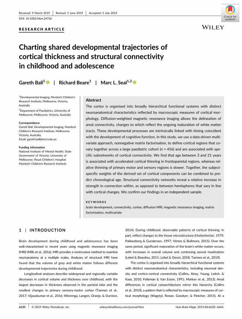
F IGURE 1 Reconstruction error and age prediction for increasing number of NMF components. (a) Reconstruction errors (RMSE; root meansquared error in terms of Euclidean-normed cortical thickness or connectivity values), averaged over 5 Wold holdouts, for cortical thickness (left)and structural connectivity data (right). Error for training datapoints (blue) and held-out test datapoints (green) are shown with 95% C.I. (b) Meanabsolute error in age prediction is shown, averaged over 10 cross-validation folds for each set of NMF components. (c) Individual age predictionsare shown for each set of components [Color figure can be viewed at wileyonlinelibrary.com]

4634 BALL ET AL.

(Figure 1b). Figure 1c shows individual, cross-validated predictions of

age based on each of the NMF component sets. Mean absolute error

in age estimation was similar across all component sets with the low-

est error observed in the 10 component set (mean MAE ± S.D = 2.18

± 0.18) and highest in the 20 component set (2.60 ± 0.30).

As reconstruction errors and age prediction were relatively similar

between component sets, we initially progress by focusing on the five

component set only. For comparison, decompositions of cortical thick-

ness and structural connectivity into 2, 5, and 10 components are

shown in Figure S1.

3.2 | Cortical thickness components

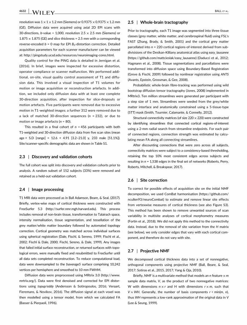
Figure 2 shows the result of projective NMF decomposition of cortical

thickness data into five components, along with corresponding com-

ponent timecourses. Each image represents the spatial distribution of

component weights across the cortex, highlighting regions that vary

across the population together. Each map is associated with a timecourse

that describes the relative contribution of that component to the full

data set and reflects how cortical thickness within the regions described

by each map varies over time.

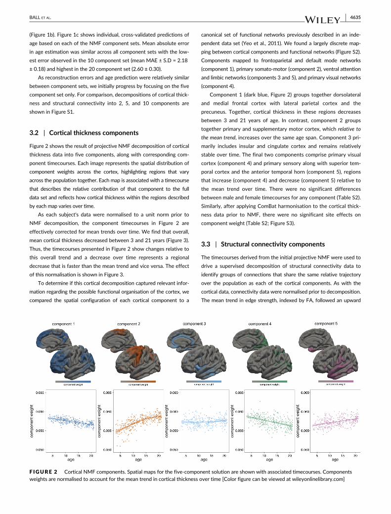
As each subject's data were normalised to a unit norm prior to

NMF decomposition, the component timecourses in Figure 2 are

effectively corrected for mean trends over time. We find that overall,

mean cortical thickness decreased between 3 and 21 years (Figure 3).

Thus, the timecourses presented in Figure 2 show changes relative to

this overall trend and a decrease over time represents a regional

decrease that is faster than the mean trend and vice versa. The effect

of this normalisation is shown in Figure 3.

To determine if this cortical decomposition captured relevant infor-

mation regarding the possible functional organisation of the cortex, we

compared the spatial configuration of each cortical component to a

canonical set of functional networks previously described in an inde-

pendent data set (Yeo et al., 2011). We found a largely discrete map-

ping between cortical components and functional networks (Figure S2).

Components mapped to frontoparietal and default mode networks

(component 1), primary somato-motor (component 2), ventral attention

and limbic networks (components 3 and 5), and primary visual networks

(component 4).

Component 1 (dark blue, Figure 2) groups together dorsolateral

and medial frontal cortex with lateral parietal cortex and the

precuneus. Together, cortical thickness in these regions decreases

between 3 and 21 years of age. In contrast, component 2 groups

together primary and supplementary motor cortex, which relative to

the mean trend, increases over the same age span. Component 3 pri-

marily includes insular and cingulate cortex and remains relatively

stable over time. The final two components comprise primary visual

cortex (component 4) and primary sensory along with superior tem-

poral cortex and the anterior temporal horn (component 5), regions

that increase (component 4) and decrease (component 5) relative to

the mean trend over time. There were no significant differences

between male and female timecourses for any component (Table S2).

Similarly, after applying ComBat harmonisation to the cortical thick-

ness data prior to NMF, there were no significant site effects on

component weight (Table S2; Figure S3).

3.3 | Structural connectivity components

The timecourses derived from the initial projective NMF were used to

drive a supervised decomposition of structural connectivity data to

identify groups of connections that share the same relative trajectory

over the population as each of the cortical components. As with the

cortical data, connectivity data were normalised prior to decomposition.

The mean trend in edge strength, indexed by FA, followed an upward

F IGURE 2 Cortical NMF components. Spatial maps for the five-component solution are shown with associated timecourses. Componentsweights are normalised to account for the mean trend in cortical thickness over time [Color figure can be viewed at wileyonlinelibrary.com]

BALL ET AL. 4635

course, increasing rapidly to around 12 years before plateauing.

The mean trend and raw (unnormalised) component timecourses

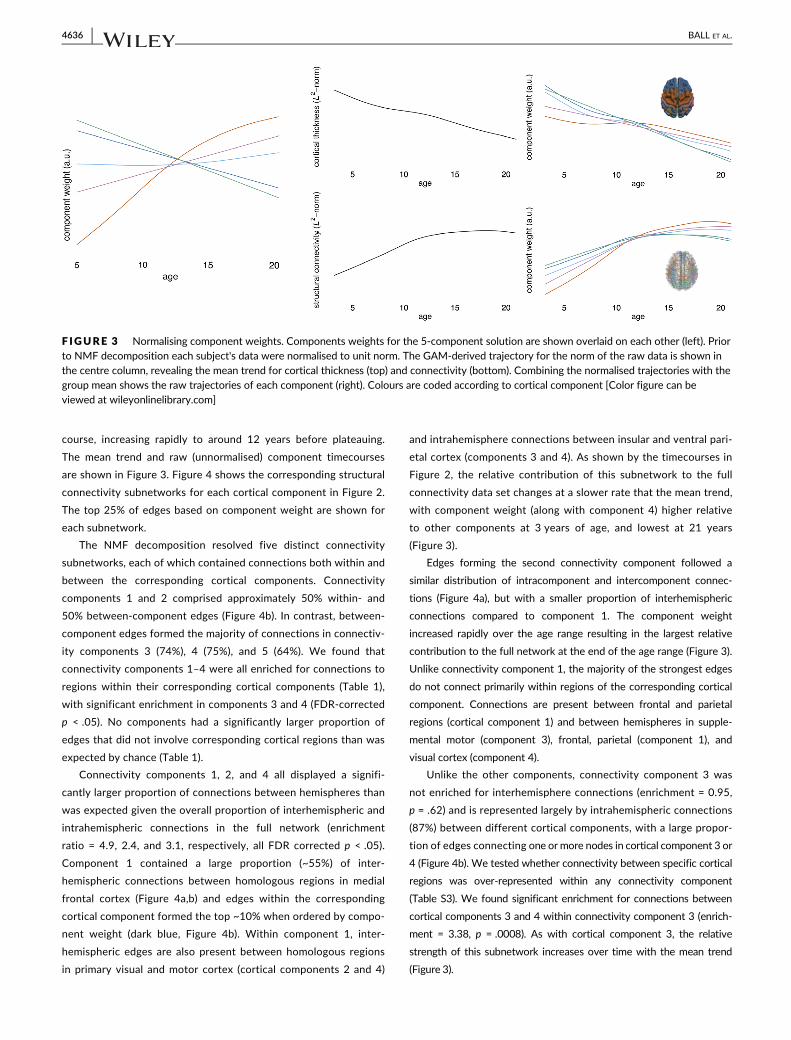
are shown in Figure 3. Figure 4 shows the corresponding structural

connectivity subnetworks for each cortical component in Figure 2.

The top 25% of edges based on component weight are shown for

each subnetwork.

The NMF decomposition resolved five distinct connectivity

subnetworks, each of which contained connections both within and

between the corresponding cortical components. Connectivity

components 1 and 2 comprised approximately 50% within- and

50% between-component edges (Figure 4b). In contrast, between-

component edges formed the majority of connections in connectiv-

ity components 3 (74%), 4 (75%), and 5 (64%). We found that

connectivity components 1–4 were all enriched for connections to

regions within their corresponding cortical components (Table 1),

with significant enrichment in components 3 and 4 (FDR-corrected

p < .05). No components had a significantly larger proportion of

edges that did not involve corresponding cortical regions than was

expected by chance (Table 1).

Connectivity components 1, 2, and 4 all displayed a signifi-

cantly larger proportion of connections between hemispheres than

was expected given the overall proportion of interhemispheric and

intrahemispheric connections in the full network (enrichment

ratio = 4.9, 2.4, and 3.1, respectively, all FDR corrected p < .05).

Component 1 contained a large proportion (~55%) of inter-

hemispheric connections between homologous regions in medial

frontal cortex (Figure 4a,b) and edges within the corresponding

cortical component formed the top ~10% when ordered by compo-

nent weight (dark blue, Figure 4b). Within component 1, inter-

hemispheric edges are also present between homologous regions

in primary visual and motor cortex (cortical components 2 and 4)

and intrahemisphere connections between insular and ventral pari-

etal cortex (components 3 and 4). As shown by the timecourses in

Figure 2, the relative contribution of this subnetwork to the full

connectivity data set changes at a slower rate that the mean trend,

with component weight (along with component 4) higher relative

to other components at 3 years of age, and lowest at 21 years

(Figure 3).

Edges forming the second connectivity component followed a

similar distribution of intracomponent and intercomponent connec-

tions (Figure 4a), but with a smaller proportion of interhemispheric

connections compared to component 1. The component weight

increased rapidly over the age range resulting in the largest relative

contribution to the full network at the end of the age range (Figure 3).

Unlike connectivity component 1, the majority of the strongest edges

do not connect primarily within regions of the corresponding cortical

component. Connections are present between frontal and parietal

regions (cortical component 1) and between hemispheres in supple-

mental motor (component 3), frontal, parietal (component 1), and

visual cortex (component 4).

Unlike the other components, connectivity component 3 was

not enriched for interhemisphere connections (enrichment = 0.95,

p = .62) and is represented largely by intrahemispheric connections

(87%) between different cortical components, with a large propor-

tion of edges connecting one or more nodes in cortical component 3 or

4 (Figure 4b). We tested whether connectivity between specific cortical

regions was over-represented within any connectivity component

(Table S3). We found significant enrichment for connections between

cortical components 3 and 4 within connectivity component 3 (enrich-

ment = 3.38, p = .0008). As with cortical component 3, the relative

strength of this subnetwork increases over time with the mean trend

(Figure 3).

F IGURE 3 Normalising component weights. Components weights for the 5-component solution are shown overlaid on each other (left). Priorto NMF decomposition each subject's data were normalised to unit norm. The GAM-derived trajectory for the norm of the raw data is shown inthe centre column, revealing the mean trend for cortical thickness (top) and connectivity (bottom). Combining the normalised trajectories with thegroup mean shows the raw trajectories of each component (right). Colours are coded according to cortical component [Color figure can beviewed at wileyonlinelibrary.com]

4636 BALL ET AL.

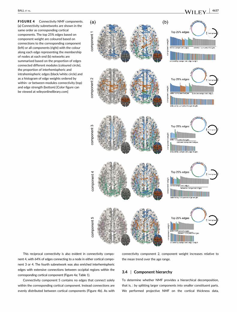
This reciprocal connectivity is also evident in connectivity compo-

nent 4, with 64% of edges connecting to a node in either cortical compo-

nent 3 or 4. The fourth subnetwork was also enriched interhemispheric

edges with extensive connections between occipital regions within the

corresponding cortical component (Figure 4a; Table 1).

Connectivity component 5 contains no edges that connect solely

within the corresponding cortical component. Instead connections are

evenly distributed between cortical components (Figure 4b). As with

connectivity component 2, component weight increases relative to

the mean trend over the age range.

3.4 | Component hierarchy

To determine whether NMF provides a hierarchical decomposition,

that is, : by splitting larger components into smaller constituent parts.

We performed projective NMF on the cortical thickness data,

F IGURE 4 Connectivity NMF components.(a) Connectivity subnetworks are shown in thesame order as corresponding corticalcomponents. The top 25% edges based oncomponent weight are coloured based onconnections to the corresponding component(left) or all components (right) with the colouralong each edge representing the membershipof nodes at each end (b) networks aresummarised based on the proportion of edgesconnected different modules (coloured circle),the proportion of interhemispheric andintrahemispheric edges (black/white circle) andas a histogram of edge weights ordered bywithin- or between-modules connectivity (top)and edge strength (bottom) [Color figure canbe viewed at wileyonlinelibrary.com]

BALL ET AL. 4637

specifying 20 components and clustered the cortical maps and

corresponding structural connectivity networks according to a hierar-

chical clustering of the component timecourses (Figure 5). There was

a significant correlation between timecourse similarity over the

20 components and distance along the clustering dendrogram

(cophenetic correlation = 0.66, p < .001 10,000 random permuta-

tions). By combining maps and networks from the higher level decom-

position according to the hierarchical clustering algorithm, we were

able to recapture patterns derived from NMF decompositions at

coarser levels (2, 5, and 10 components (Figure 5b,c) demonstrating a

stable, hierarchical decomposition of both data sets.

3.5 | Association with cognitive performance

Using neurocognitive scores from the NTCB, we tested for associa-

tions between component weight and cognitive performance. Initial

models showed age accounted for a significant proportion of variance

(R2: 0.41–0.60) in each cognitive score (Table S4). After accounting

for variation due to age and sex, standardised, residualised cognitive

scores were combined using PCA, with the first 2 principal compo-

nents (PCs) together explaining >55% of the remaining variance. After

FDR correction to account for multiple tests, we found two significant

linear associations between the second PC and NMF components

1 and 4. These results showed a small positive correlation (R2 = 0.03,

p = .008) between relatively slower thinning in frontal and parietal

regions and improved performance in attention-related tasks and rela-

tively poorer performance in vocabulary and reading tasks with the

opposite relationship (R2 = 0.03, p = .005) in component 4 (visual and

lateral parietal cortex) (Figure S4).

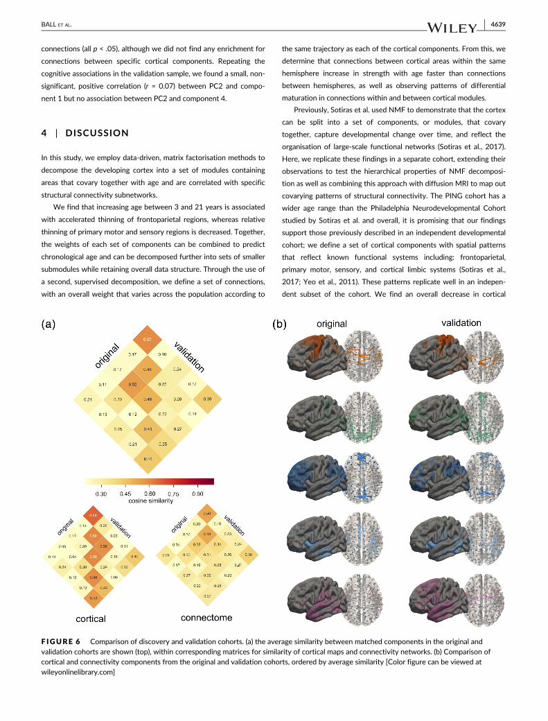
3.6 | Validation cohort

For validation, we repeated the NMF decomposition of cortical thick-

ness and structural connectivity data into five components in the

remaining, held-out subsample (n = 152). The similarity of the resul-

tant cortical maps and connectivity subnetworks are shown in

Figure 6, ordered by average similarity to matched components in the

discovery cohort. Average cosine similarity was significantly higher

between matched components compared to unmatched (t = 4.83,

p < .001) and ranged from 0.4 (component 5) to 0.57 (component 2).

Matching was performed separately for cortical and connectivity com-

ponents; similarity was higher for cortical thickness maps (range:

0.53–0.64; matched vs. unmatched: t = 5.75, p < .001) compared to

connectivity subnetworks (0.27–0.50; t = 3.24, p = .004). Component

timecourses were similar between discovery and validation samples

(Figure S5). We also found similar patterns of edge enrichment in the

network components with enrichment for edges connected to

corresponding cortical component in network components 1 and

2 (enrichment = 1.24, 2.48; p = .09, p = .00002*, respectively, *FDR

corrected p < .05) and all components enriched for interhemispheric

TABLE 1 Enrichment of connectivity component edges forconnections to corresponding cortical components

Connected tocortical component

Not connected tocortical component

Component Enrichment p Enrichment p

1 1.19 .091 0.86 .94

2 1.32 .074 0.92 .95

3 1.57 .0021a 0.68 .99

4 1.58 .0005a 0.73 .99

5 0.92 .674 1.03 .45

aFDR corrected p < .05.

F IGURE 5 Hierarchical decomposition of NMF components. (a) 20 NMF components are clustered based on similarity of component weightsacross subjects. (b) The spatial similarity between NMF decompositions at a level of 2 components are shown with maps constructed through theaddition of hierarchically clustered components at lower levels. (c) Similarity matrices are shown at the 5 and 10 component level [Color figurecan be viewed at wileyonlinelibrary.com]

4638 BALL ET AL.

connections (all p < .05), although we did not find any enrichment for

connections between specific cortical components. Repeating the

cognitive associations in the validation sample, we found a small, non-

significant, positive correlation (r = 0.07) between PC2 and compo-

nent 1 but no association between PC2 and component 4.

4 | DISCUSSION

In this study, we employ data-driven, matrix factorisation methods to

decompose the developing cortex into a set of modules containing

areas that covary together with age and are correlated with specific

structural connectivity subnetworks.

We find that increasing age between 3 and 21 years is associated

with accelerated thinning of frontoparietal regions, whereas relative

thinning of primary motor and sensory regions is decreased. Together,

the weights of each set of components can be combined to predict

chronological age and can be decomposed further into sets of smaller

submodules while retaining overall data structure. Through the use of

a second, supervised decomposition, we define a set of connections,

with an overall weight that varies across the population according to

the same trajectory as each of the cortical components. From this, we

determine that connections between cortical areas within the same

hemisphere increase in strength with age faster than connections

between hemispheres, as well as observing patterns of differential

maturation in connections within and between cortical modules.

Previously, Sotiras et al. used NMF to demonstrate that the cortex

can be split into a set of components, or modules, that covary

together, capture developmental change over time, and reflect the

organisation of large-scale functional networks (Sotiras et al., 2017).

Here, we replicate these findings in a separate cohort, extending their

observations to test the hierarchical properties of NMF decomposi-

tion as well as combining this approach with diffusion MRI to map out

covarying patterns of structural connectivity. The PING cohort has a

wider age range than the Philadelphia Neurodevelopmental Cohort

studied by Sotiras et al. and overall, it is promising that our findings

support those previously described in an independent developmental

cohort; we define a set of cortical components with spatial patterns

that reflect known functional systems including: frontoparietal,

primary motor, sensory, and cortical limbic systems (Sotiras et al.,

2017; Yeo et al., 2011). These patterns replicate well in an indepen-

dent subset of the cohort. We find an overall decrease in cortical

F IGURE 6 Comparison of discovery and validation cohorts. (a) the average similarity between matched components in the original andvalidation cohorts are shown (top), within corresponding matrices for similarity of cortical maps and connectivity networks. (b) Comparison ofcortical and connectivity components from the original and validation cohorts, ordered by average similarity [Color figure can be viewed atwileyonlinelibrary.com]

BALL ET AL. 4639

thickness with age (Figure 3), this support recent findings in multiple

longitudinal cohorts demonstrating a broadly monotonic decrease in

thickness over time in the same age range (Tamnes et al., 2017). After

correcting for this mean trend, we observe regional differences in rate

of change in thickness across cortical components. In contrast to

Sotiras et al., where raw (not normalised) cortical data were used for

NMF, no differences were observed between sexes in component tra-

jectory, suggesting any sex differences were captured by the differ-

ences in mean thickness. Focusing on the five component model, we

find that cortical thinning was fastest in components 1 and 4 compris-

ing regions in dorsolateral frontal and parietal cortex, precuneus and

primary visual cortex, and slowest in primary and supplementary

motor, primary sensory and superior temporal cortex. Regional model-

ling of cortical thickness has found similar patterns, broadly respecting

the organisational hierarchy of the cortex (Fjell et al., 2015; Tamnes

et al., 2010, 2017; Vijayakumar et al., 2016). The differential rate of

thinning is greatest in association cortex (component 1) compared to

primary motor and sensory regions (components 2 and 5), with the

exception of the visual cortex (component 4). We anticipate these dif-

ferences in regional rate of change reflects the differential progress of

microstructural processes including synaptic pruning (Huttenlocher,

1979), although recent evidence has suggested that apparent cortical

thinning in the visual cortex may be dependent on tissue contrast

changes due to intracortial myelination, rather than synaptic

remodelling (Natu et al., 2018).

Our use of supervised NMF to derive a corresponding set of con-

nectivity subnetworks that covary over the population in line with

each cortical component allow the direct comparison of cortical and

white matter development. Other studies have employed different

methods to study concomitant changes across both tissue compart-

ments. These approaches include inspection and comparison of white

matter properties directly subjacent to different cortical regions

(Croteau-Chonka et al., 2016), or examination of white matter tracts

from specific cortical gyri (Jeon, Mishra, Ouyang, Chen, & Huang,

2015) or connections between cortical areas that displaying signifi-

cant age-related changes in surface area in childhood (Cafiero, Brauer,

Anwander, & Friederici, 2019). A strength of our approach is that we

used a data-driven method to select important connections based on

their covariation with each cortical component. This allows the deriva-

tion of spatially (topologically) independent subnetworks, where con-

nections are not shared between components, that vary together

across the population (Ball, Beare, & Seal, 2017). Importantly, this

form of supervised decomposition can be applied to any data set,

imaging or otherwise, that is (or has been transformed to be) nonneg-

ative and is shared by the same participants.

In contrast to previous approaches, this method does not restrict

white matter connections to those that exclusively connect to the

corresponding cortical component, instead selecting groups of edges

where change over time relative to the mean trend mirrors that seen

in the cortex. The mean trend in connectivity strength revealed a rela-

tively quick increase that slows at around 12 years reaching a plateau

by late adolescence. Similar trends in white matter maturation, as

indexed by FA, have been described previously using tractographic

approaches (Chen, Zhang, Yushkevich, Liu, & Beaulieu, 2016). Overall,

connectivity component 2 showed the most rapid increases, with

components 1 and 4 the slowest.

Connectivity component 1 exhibited the largest proportion of

within-module connections and was significantly enriched for connec-

tions to/from regions within its corresponding cortical component, with

a large proportion of edges between homologous regions in frontal and

parietal cortex. There were significantly more edges within this compo-

nent connecting between hemispheres and, as with the cortical compo-

nent, the relative contribution of these edges to the full network

decreases with age, rising slowest between 3 and 21 years. In contrast,

connectivity component 2 contained a lower proportion of inter-

hemispheric connections (though still more than expected by chance)

with edges that show the largest increase with age and connecting pre-

dominately within hemisphere. Similarly, edge strength within compo-

nent 5 increases rapidly with age, plateauing later than components

1 or 4. Edges were not significantly enriched for between-hemisphere

connections and were predominantly within hemisphere These findings

support observations from diffusion tractography studies that found

that interhemispheric commissural tracts display earlier maturation

compared to within-hemisphere association fibres such as the superior

longitudinal and fronto-occipital fasciculi (Lebel & Beaulieu, 2011).

A large proportion of reciprocal connectivity was observed between

subnetworks associated with the spatially adjacent cortical components

3 and 4, supported by connection within connectivity component

3, with a number of edges connecting one areas in each component,

although the cortical components showed differential change over

time. Component 4, comprising a larger portion of interhemispheric

edges decreasing in strength relative to the mean compared to com-

ponent 3. Connectivity component 5 was the only network that was

not significantly enriched for edges connecting to its corresponding

cortical component. This relatively distributed subnetwork con-

tained edges connecting to all cortical components, predominately

within hemisphere. Therefore, this component may represent an

integrative network process that facilitates communication across

the network and have been shown to increase during adolescence

(Dennis et al., 2013).

Using our NMF approach, we found that changes in focal cortical

components were associated with contemporaneous changes in rela-

tively distributed connectivity subnetworks. As the cortical and con-

nectivity components were linked by a shared timecourse, this likely

reflects a combination of developmental processes occurring simulta-

neously within the brain. Cafiero et al. recently demonstrated that

streamlines passing through regions of myelinating white matter in

early childhood terminate within large swathes of the developing cor-

tex (Cafiero et al., 2019). We chose FA to define white matter connec-

tivity strength, a partial proxy for white matter myelination in the

developing brain (Lebel & Beaulieu, 2011). As such, developmental

changes in the core white matter, through which all major white mat-

ter tracts pass will likely impact a wide range of structural network

connections. Despite this, we identified specialised networks with

preferential connections to corresponding cortical regions in 4 out of

5 components. We suggest that this likely reflects the differential

4640 BALL ET AL.

developmental trajectories of major tract systems that carry connec-

tions to/from focal cortical regions (Lebel & Beaulieu, 2011).

To test whether individual variance in regional cortical develop-

ment was associated with neurocognitive parameters, we performed

an additional analysis examining association between component

weight and performance on a suite of cognitive tests. We found only

weak associations between differential thinning in frontparietal regions

(component 1) and visual and lateral parietal regions (component 4) and

performance, that did not explain susbstantial variance in the cognitive

score. Indeed, as with previous studies in this cohort, we found that

age accounted for the majority of individual variance (Akshoomoff

et al., 2014), whereas only a small degree of variation could additionally

be accounted for by neuroanatomical measures, after correcting for age

(Ball, Adamson, et al., 2017). This analysis does not provide strong sup-

port for a relationship between regional patterns of relative cortical

thickness and cognitive performance but, as noted by Akshoomoff

et al., the large age range of the PING cohort means that the majority

of variance in the data will be accounted for by age differences. This

conclusion would benefit from additional studies designed to compare

performance within larger cohorts across a smaller age range, such as

the ongoing ABCD study (Casey et al., 2018).

As is often the case with unsupervised methods, the appropriate

choice of component number poses a difficult challenge. We per-

formed NMF using five different levels: 2, 5, 10, 15, and 20 and com-

pared how well the resulting components could reconstruct the

original data, and how well the resulting timecourses could be used to

predict chronological age. Overall, we did not find significant differ-

ences between the different levels of resolution. Reconstruction error

was relatively stable across all component sets, as was age prediction

error for all levels except for n = 20. Overall, age prediction error was

in range with previous “brain age” estimates (Ball, Adamson, et al.,

2017; Cole et al., 2017; Franke, Luders, May, Wilke, & Gaser, 2012)

confirming that utility of NMF for providing useful low-rank represen-

tations of large imaging data sets (Varikuti et al., 2018).

As the prediction errors were relatively stable, we chose to focus

on the five component set for ease of interpretation. We provide

additional images of cortical and network components in Figure S1

for comparison. We also note that, using split-half repeats as a mea-

sure of reliability, Sotiras et al. found the most reliable decomposi-

tions at similarly coarse levels (2, 7, and 18). The fact that

reconstruction error did not significantly change when increasing the

number of components suggested that the bulk of the original data

matrix was captured by the lowest level of decomposition (i.e., two

components), and that increasing the decomposition resolution fur-

ther resulted in a subdivision of these two, larger components. To

test this hypothesis, we performed a hierarchical clustering of the

highest resolution decomposition, combining cortical and connectiv-

ity components based on the similarity of their timecourses. We

found that there was significant hierarchical structure in the NMF

decompositions and could largely recapture the original

2-component solution by combining a number of smaller compo-

nents (Figure 4). This may allow future studies to compare findings

even if different numbers of components are specified.

We suspect that the broadly hierarchical decomposition may also

explain why cortical error reconstruction did not improve with

increasing numbers of components as may be expected (Figure 1a).

We note that the RMSE for two or five components is not signifi-

cantly different and we think this behaviour, in part, reflects that the

same information is captured with 2 as with 5 components, as the

lower resolution components can be viewed as a weighted combina-

tion of the components resulting from the higher resolution decompo-

sition. Further understanding of this behaviour may be gained through

the use of multilayer NMF methods that respect the hierarchical

structure of the data (Cichocki & Zdunek, 2007).

Finally, we performed a within-cohort validation, running the

NMF decompositions separately in a held-out subset of the full

cohort. We found that, in general, similar spatial maps were defined in

the validation set. Similarity was higher in the cortical components

compared to the connectivity components, suggesting that the

decomposition of the connectivity data may be more variable, or more

dependent on sample size.

We note some limitations to this work. Firstly, there are a number

of considerations when performing structural connectivity analysis:

how to parcellate the brain, which algorithm to use for tractography,

how to threshold the connectivity matrix. However, it remains unclear

which methods are the best choice for structural connectivity ana-

lyses (Zalesky et al., 2010, 2016) We were limited in our choices in

some respect due to the lack of high angular resolution diffusion data.

Our method took advantage of state-of-the-art approaches to limit

false positives, including the use of anatomical constraints (Smith

et al., 2012), we also thresholded our matrices based on a measure of

edge weight consistency shown to improve estimate of consistent

networks across subjects (Roberts et al., 2017). While this process

may reduce the subject-level variability in the group, we view it as an

essential step to remove possible noise sources from the data. Chang-

ing the threshold would result in a slightly different set of edges and

therefore altered network components, though we anticipate that the

core patterns shown in Figure 5 would be retained. Indeed, we have

previously found this when investigating the effects of changing the

initial edge thresholds before NMF decomposition of network data

(Ball, Beare, & Seal, 2017). Secondly, we used a large multisite cohort

for this study. Site and scanner variance can impact neuroanatomical

measures derived from MRI (Fortin et al., 2018; Schnack et al., 2010).

Here, we employed a method for control of batch effects, ComBat,

and found that unwanted site variance was significantly less apparent

within component timecourses (Figure S3). We did not apply this form

of site correction to the connectivity data as, although this method

had been applied to parametric diffusion maps, for example, : FA

(Fortin et al., 2017), inter-site variation may affect the initial whole-

brain tractography prior to FA weighting. Instead, due to the removal

of site variation from the H matrix, we only consider edges that vary

with each cortical component, and therefore do not vary with site.

Due to this, we were not able to perform our method in the reverse

direction, performing PNMF first in the connectivity data, followed by

supervised NMF of the cortical data. Additionally, this study is cross-

sectional and our conclusions would be strengthened by observing

BALL ET AL. 4641

within subject longitudinal changes that mirror the cross-sectional

age-related trends reported here.

In summary, we use a data-driven, multivariate method to identify

patterns of regional cortical development that have a hierarchical

structure and reliable identified across independent cohorts. We find

that these components share developmental trajectories with distinct

subnetworks of structural connectivity.

ACKNOWLEDGMENTS

This research was conducted within the Developmental Imaging

research group, Murdoch Childrens Research Institute and the Chil-

dren's MRI Centre, Royal Children's Hospital, Melbourne, Victoria. It

was supported by the Murdoch Childrens Research Institute, the Royal

Children's Hospital, Department of Paediatrics, The University of Mel-

bourne and the State Government of Victoria‘s Operational Infrastruc-

ture Support Program. The project was generously supported by

RCH1000, a unique arm of The Royal Children's Hospital Foundation

devoted to raising funds for research at The Royal Children's Hospital.

Data and/or research tools used in the preparation of this manuscript

were obtained and analysed from the controlled access data sets

distributed from the NIMH-supported Research Domain Criteria Data-

base (RDoCdb). RDoCdb is a collaborative informatics system created by

the National Institute of Mental Health to store and share data resulting

from grants funded through the Research Domain Criteria (RDoC)

project. Dataset identifier(s): [DOI: 10.15154/1503353].

ORCID

Gareth Ball https://orcid.org/0000-0003-3509-1435

Marc L. Seal https://orcid.org/0000-0002-8396-140X

REFERENCES

Akshoomoff, N., Newman, E., Thompson, W. K., McCabe, C., Bloss, C. S.,

Chang, L., … Jernigan, T. L. (2014). The NIH toolbox cognition battery:

Results from a large normative developmental sample (PING). Neuro-

psychology, 28, 1–10.Andersson, J. L. R., & Sotiropoulos, S. N. (2016). An integrated approach to

correction for off-resonance effects and subject movement in diffu-

sion MR imaging. NeuroImage, 125, 1063–1078.Avants, B. B., Epstein, C. L., Grossman, M., & Gee, J. C. (2008). Symmetric

diffeomorphic image registration with cross-correlation: Evaluating

automated labeling of elderly and neurodegenerative brain. Medical

Image Analysis, 12, 26–41.Ball, G., Adamson, C., Beare, R., & Seal, M. L. (2017). Modelling neuroana-

tomical variation during childhood and adolescence with neighbourhood-

preserving embedding. Scientific Reports, 7, 17796.

Ball, G., Beare, R., & Seal, M. L. (2017). Network component analysis

reveals developmental trajectories of structural connectivity and spe-

cific alterations in autism spectrum disorder. Human Brain Mapping,

38, 4169–4184.Basser, P. J., & Pierpaoli, C. (1996). Microstructural and physiological fea-

tures of tissues elucidated by quantitative-diffusion-tensor MRI. Jour-

nal of Magnetic Resonance. Series B, 111, 209–219.Baum, G. L., Ciric, R., Roalf, D. R., Betzel, R. F., Moore, T. M.,

Shinohara, R. T., … Satterthwaite, T. D. (2017). Modular segregation of

structural brain networks supports the development of executive

function in youth. Current Biology, e8, 1561–1572.Beckmann, C. F., & Smith, S. M. (2005). Tensorial extensions of indepen-

dent component analysis for multisubject FMRI analysis. NeuroImage,

25, 294–311.Beul, S. F., & Hilgetag, C. C. (2019). Neuron density fundamentally relates

to architecture and connectivity of the primate cerebral cortex.

NeuroImage, 189, 777–792.Blakemore, S.-J., & Choudhury, S. (2006). Development of the adolescent

brain: Implications for executive function and social cognition. Journal

of Child Psychology and Psychiatry, 47, 296–312.Brown, T. T., Kuperman, J. M., Chung, Y., Erhart, M., McCabe, C.,

Hagler, D. J., … Dale, A. M. (2012). Neuroanatomical assessment of

biological maturity. Current Biology, 22, 1693–1698.Bullmore, E., & Sporns, O. (2012). The economy of brain network organiza-

tion. Nature Reviews. Neuroscience, 13, 336–349.Cafiero, R., Brauer, J., Anwander, A., & Friederici, A. D. (2019). The concur-

rence of cortical surface area expansion and white matter myelination

in human brain development. Cerebral Cortex, 29, 827–837.Cahalane, D. J., Charvet, C. J., & Finlay, B. L. (2012). Systematic, balancing

gradients in neuron density and number across the primate isocortex.

Frontiers in Neuroanatomy, 6(28). https://doi.org/10.3389/fnana.2012.

00028

Calhoun, V. D., Liu, J., & Adalı, T. (2009). A review of group ICA for fMRI

data and ICA for joint inference of imaging, genetic, and ERP data.

NeuroImage, 45, S163–S172.Casey, B. J., Cannonier, T., Conley, M. I., Cohen, A. O., Barch, D. M.,

Heitzeg, M. M., … Dale, A. M. (2018). The adolescent brain cognitive

development (ABCD) study: Imaging acquisition across 21 sites. Dev

Cogn Neurosci, the Adolescent Brain Cognitive Development (ABCD) Con-

sortium: Rationale, Aims, and Assessment Strategy., 32, 43–54.Chen, Z., Zhang, H., Yushkevich, P. A., Liu, M., & Beaulieu, C. (2016). Matu-

ration along white matter tracts in human brain using a diffusion tensor

surface model tract-specific analysis. Frontiers in Neuroanatomy, 10(9).

https://doi.org/10.3389/fnana.2016.00009

Cichocki, A., & Zdunek, R. (2007). Multilayer nonnegative matrix factoriza-

tion using projected gradient approaches. International Journal of Neu-

ral Systems, 17, 431–446.Cole, J. H., Poudel, R. P. K., Tsagkrasoulis, D., Caan, M. W. A., Steves, C.,

Spector, T. D., & Montana, G. (2017). Predicting brain age with deep

learning from raw imaging data results in a reliable and heritable bio-

marker. NeuroImage, 163, 115–124.Collins, C. E., Airey, D. C., Young, N. A., Leitch, D. B., & Kaas, J. H. (2010).

Neuron densities vary across and within cortical areas in primates. Pro-

ceedings of the National Academy of Sciences of the United States of

America, 107, 15927–15932.Croteau-Chonka, E. C., Dean, D. C., Remer, J., Dirks, H., O'Muircheartaigh, J., &

Deoni, S. C. L. (2016). Examining the relationships between cortical matura-

tion andwhitemattermyelination throughout early childhood.NeuroImage,

125, 413–421.Daducci, A., Gerhard, S., Griffa, A., Lemkaddem, A., Cammoun, L.,

Gigandet, X., … Thiran, J.-P. (2012). The connectome mapper: An

open-source processing pipeline to map connectomes with MRI. PLoS

One, 7, e48121.

Dale, A. M., Fischl, B., & Sereno, M. I. (1999). Cortical surface-based analy-

sis: I. segmentation and surface reconstruction. NeuroImage, 9,

179–194.Dennis, E. L., Jahanshad, N., McMahon, K. L., de Zubicaray, G. I.,

Martin, N. G., Hickie, I. B., … Thompson, P. M. (2013). Development of

brain structural connectivity between ages 12 and 30: A 4-tesla diffu-

sion imaging study in 439 adolescents and adults. NeuroImage, 64,

671–684.Van Essen, D. C. (1997). A tension-based theory of morphogenesis and

compact wiring in the central nervous system. Nature, 385, 313–318.

4642 BALL ET AL.

Faskowitz, J., Yan, X., Zuo, X.-N., & Sporns, O. (2018). Weighted stochastic

block models of the human connectome across the life span. Scientific

Reports, 8, 12997.

Felleman, D. J., & Van Essen, D. C. (1991). Distributed hierarchical

processing in the primate cerebral cortex. Cerebral Cortex, 1991, 1:

1–1:47.Fischl, B., & Dale, A. M. (2000). Measuring the thickness of the human

cerebral cortex from magnetic resonance images. Proceedings of the

National Academy of Sciences of the United States of America, 97,

11050–11055.Fischl, B., Salat, D. H., Busa, E., Albert, M., Dieterich, M., Haselgrove, C., …

Dale, A. M. (2002). Whole brain segmentation: Automated labeling of

neuroanatomical structures in the human brain. Neuron, 33, 341–355.Fischl, B., Sereno, M. I., & Dale, A. M. (1999). Cortical surface-based analy-

sis: II: Inflation, flattening, and a surface-based coordinate system.

NeuroImage, 9, 195–207.Fjell, A. M., Grydeland, H., Krogsrud, S. K., Amlien, I., Rohani, D. A.,

Ferschmann, L., … Walhovd, K. B. (2015). Development and aging of

cortical thickness correspond to genetic organization patterns. Pro-

ceedings of the National Academy of Sciences of the United States of

America, 112, 15462–15467.Fortin, J.-P., Cullen, N., Sheline, Y. I., Taylor, W. D., Aselcioglu, I.,

Cook, P. A., … Shinohara, R. T. (2018). Harmonization of cortical thick-

ness measurements across scanners and sites. NeuroImage, 167,

104–120.Fortin, J.-P., Parker, D., Tunç, B., Watanabe, T., Elliott, M. A., Ruparel, K., …

Shinohara, R. T. (2017). Harmonization of multi-site diffusion tensor

imaging data. NeuroImage, 161, 149–170.Franke, K., Luders, E., May, A., Wilke, M., & Gaser, C. (2012). Brain matura-

tion: Predicting individual BrainAGE in children and adolescents using

structural MRI. NeuroImage, 63, 1305–1312.Greve, D. N., & Fischl, B. (2009). Accurate and robust brain image align-

ment using boundary-based registration. NeuroImage, 48, 63–72.Groves, A. R., Beckmann, C. F., Smith, S. M., & Woolrich, M. W. (2011).

Linked independent component analysis for multimodal data fusion.

NeuroImage, 54, 2198–2217.Hagmann, P., Cammoun, L., Gigandet, X., Meuli, R., Honey, C. J.,

Wedeen, V. J., & Sporns, O. (2008). Mapping the structural core of

human cerebral cortex. PLoS Biology, 6, e159.

Herculano-Houzel, S., Mota, B., Wong, P., & Kaas, J. H. (2010). Connectiv-

ity-driven white matter scaling and folding in primate cerebral cortex.

Proceedings of the National Academy of Sciences of the United States of

America, 107, 19008–19013.Hilgetag, C.-C., Burns, G. A. P. C., O'Neill, M. A., Scannell, J. W., &

Young, M. P. (2000). Anatomical connectivity defines the organization

of clusters of cortical areas in the macaque and the cat. Philosophical

Transactions of the Royal Society of London. Series B, Biological Sciences,

355, 91–110.Huttenlocher, P. R. (1979). Synaptic density in human frontal cortex -

developmental changes and effects of aging. Brain Research, 163,

195–205.Jeon, T., Mishra, V., Ouyang, M., Chen, M., & Huang, H. (2015). Synchro-

nous changes of cortical thickness and corresponding white matter

microstructure during brain development accessed by diffusion MRI

tractography from parcellated cortex. Frontiers in Neuroanatomy, 9

(158). https://doi.org/10.3389/fnana.2015.00158

Jernigan, T. L., Brown, T. T., Hagler, D. J., Jr., Akshoomoff, N., Bartsch, H.,

Newman, E., … Dale, A. M. (2016). The pediatric imaging, neuro-

cognition, and genetics (PING) data repository. NeuroImage, Sharing

the Wealth: Brain Imaging Repositories, 124, 1149–1154.Jones, D. K. (2008). Tractography gone wild: Probabilistic fibre tracking

using the wild bootstrap with diffusion tensor MRI. IEEE Transactions

on Medical Imaging, 27, 1268–1274.Kharitonova, M., Martin, R. E., Gabrieli, J. D. E., & Sheridan, M. A. (2013).

Cortical gray-matter thinning is associated with age-related

improvements on executive function tasks. Developmental Cognitive

Neuroscience, 6, 61–71.Krogsrud, S. K., Fjell, A. M., Tamnes, C. K., Grydeland, H., Due-

Tønnessen, P., Bjørnerud, A., … Walhovd, K. B. (2018). Development of

white matter microstructure in relation to verbal and visuospatial work-

ing memory—A longitudinal study. PLoS One, 13, e0195540.

Lebel, C., & Beaulieu, C. (2011). Longitudinal development of human brain

wiring continues from childhood into adulthood. The Journal of Neuro-

science, 31, 10937–10947.Lebel, C., & Deoni, S. (2018). The development of brain white matter

microstructure. NeuroImage, 182, 207–218.Lebel, C., Walker, L., Leemans, A., Phillips, L., & Beaulieu, C. (2008). Micro-

structural maturation of the human brain from childhood to adulthood.

NeuroImage, 40, 1044–1055.Lee, D. D., & Seung, H. S. (1999). Learning the parts of objects by non-

negative matrix factorization. Nature, 401, 788–791.Markov, N. T., Vezoli, J., Chameau, P., Falchier, A., Quilodran, R., Huissoud, C.,

… Kennedy, H. (2013). Anatomy of hierarchy: Feedforward and feedback

pathways in macaque visual cortex. The Journal of Comparative Neurology,

522, 225–259.Mills, K. L., Goddings, A.-L., Herting, M. M., Meuwese, R., Blakemore, S.-J.,

Crone, E. A., … Tamnes, C. K. (2016). Structural brain development

between childhood and adulthood: Convergence across four longitudi-

nal samples. NeuroImage, 141, 273–281.Mota, B., & Herculano-Houzel, S. (2012). How the cortex gets its folds: An

inside-out, connectivity-driven model for the scaling of mammalian

cortical folding. Frontiers in Neuroanatomy, 6(3). https://doi.org/10.

3389/fnana.2012.00003

Natu, V. S., Gomez, J., Barnett, M., Jeska, B., Kirilina, E., Jaeger, C., … Grill-

Spector, K. (2018). Apparent thinning of visual cortex during childhood

is associated with myelination, not pruning. bioRxiv, 368274. https://

doi.org/10.1101/368274

Pakkenberg, B., & Gundersen, H. J. (1997). Neocortical neuron number in

humans: Effect of sex and age. The Journal of Comparative Neurology,

384, 312–320.Roberts, J. A., Perry, A., Roberts, G., Mitchell, P. B., & Breakspear, M.

(2017). Consistency-based thresholding of the human connectome.

NeuroImage, 145, 118–129.Schnack, H. G., van Haren, N. E. M., Brouwer, R. M., van, B. G. C. M.,

Picchioni, M., Weisbrod, M., … Pol, H. E. H. (2010). Mapping reliability

in multicenter MRI: Voxel-based morphometry and cortical thickness.

Human Brain Mapping, 31, 1967–1982.Scholtens, L. H., Schmidt, R., de Reus, M. A., & van den MP, H. (2014).

Linking macroscale graph analytical organization to microscale neu-

roarchitectonics in the macaque connectome. The Journal of Neurosci-

ence, 34, 12192–12205.Schüz, A., & Palm, G. (1989). Density of neurons and synapses in the cere-

bral cortex of the mouse. The Journal of Comparative Neurology, 286,

442–455.Smith, R. E., Tournier, J.-D., Calamante, F., & Connelly, A. (2012). Anatomi-

cally-constrained tractography: Improved diffusion MRI streamlines

tractography through effective use of anatomical information.

NeuroImage, 62, 1924–1938.Sotiras, A., Resnick, S. M., & Davatzikos, C. (2015). Finding imaging pat-

terns of structural covariance via non-negative matrix factorization.

NeuroImage, 108, 1–16.Sotiras, A., Toledo, J. B., Gur, R. E., Gur, R. C., Satterthwaite, T. D., &

Davatzikos, C. (2017). Patterns of coordinated cortical remodeling dur-

ing adolescence and their associations with functional specialization and

evolutionary expansion. Proceedings of the National Academy of Sciences,

114(13), 3527–3532. https://doi.org/10.1073/pnas.1620928114Squeglia, L. M., Jacobus, J., Sorg, S. F., Jernigan, T. L., & Tapert, S. F.

(2013). Early adolescent cortical thinning is related to better neuropsy-

chological performance. Journal of the International Neuropsychological

Society, 19, 962–970.

BALL ET AL. 4643

Sui, J., Adali, T., Yu, Q., & Calhoun, V. D. (2012). A review of multivariate

methods for multimodal fusion of brain imaging data. Journal of Neuro-

science Methods, 204, 68–81.Tamnes, C. K., Herting, M. M., Goddings, A.-L., Meuwese, R., Blakemore, S.-

J., Dahl, R. E., … Mills, K. L. (2017). Development of the cerebral cortex

across adolescence: A multisample study of inter-related longitudinal

changes in cortical volume, surface area, and thickness. Journal of

Neuroscience: The Official Journal of the Society for Neuroscience, 37,

3402–3412.Tamnes, C. K., Ostby, Y., Fjell, A. M., Westlye, L. T., Due-Tønnessen, P., &

Walhovd, K. B. (2010). Brain maturation in adolescence and young

adulthood: regional age-related changes in cortical thickness and white

matter volume and microstructure. Cereberal Cortex, 20, 534–548.Varikuti, D. P., Genon, S., Sotiras, A., Schwender, H., Hoffstaedter, F.,

Patil, K. R., … Eickhoff, S. B. (2018). Evaluation of non-negative matrix fac-

torization of grey matter in age prediction. NeuroImage, 173, 394–410.Veraart, J., Fieremans, E., & Novikov, D. S. (2016). Diffusion MRI noise

mapping using random matrix theory. Magnetic Resonance in Medicine,

76, 1582–1593.Vértes, P. E., & Bullmore, E. T. (2015). Annual research review: Growth

connectomics--the organization and reorganization of brain networks

during normal and abnormal development. Journal of Child Psychology

and Psychiatry, 56, 299–320.Vijayakumar, N., Allen, N. B., Youssef, G., Dennison, M., Yücel, M.,

Simmons, J. G., & Whittle, S. (2016). Brain development during adoles-

cence: A mixed-longitudinal investigation of cortical thickness, surface

area, and volume. Human Brain Mapping, 37, 2027–2038.Wagstyl, K., Ronan, L., Goodyer, I. M., & Fletcher, P. C. (2015). Cortical thick-

ness gradients in structural hierarchies. NeuroImage, 111, 241–250.Wierenga, L. M., Langen, M., Oranje, B., & Durston, S. (2014). Unique

developmental trajectories of cortical thickness and surface area.

NeuroImage, 87, 120–126.Wold, S. (1978). Cross-validatory estimation of the number of components in

factor and principal components models. Technometrics, 20, 397–405.Wood, S. (2017). Generalized additive models: An introduction with R (2nd ed.).

Boca Raton, Florida: CRC Press.

Wood, S. N. (2003). Thin plate regression splines. Journal of the Royal Sta-

tistical Society Part B, 65, 95–114.

Wood, S. N. (2011). Fast stable restricted maximum likelihood and marginal

likelihood estimation of semiparametric generalized linear models. Jour-

nal of the Royal Statistical Society Part B, 73, 3–36.Yang, Z., & Oja, E. (2010). Linear and nonlinear projective nonnegative matrix

factorization. IEEE Transactions on Neural Networks, 21, 734–749.Yeo, B. T. T., Krienen, F. M., Sepulcre, J., Sabuncu, M. R., Lashkari, D.,

Hollinshead, M., … Buckner, R. L. (2011). The organization of the

human cerebral cortex estimated by intrinsic functional connectivity.

Journal of Neurophysiology, 106, 1125–1165.Zalesky, A., Fornito, A., Cocchi, L., Gollo, L. L., van den Heuvel, M. P., &

Breakspear, M. (2016). Connectome sensitivity or specificity: Which is

more important? NeuroImage, 142, 407–420.Zalesky, A., Fornito, A., Harding, I. H., Cocchi, L., Yücel, M., Pantelis, C., &

Bullmore, E. T. (2010). Whole-brain anatomical networks: Does the

choice of nodes matter? NeuroImage, 50, 970–983.Zhang, Y., Brady, M., & Smith, S. (2001). Segmentation of brain MR images

through a hidden Markov random field model and the expectation-

maximization algorithm. IEEE Transactions on Medical Imaging, 20, 45–57.Zhao, T., Cao, M., Niu, H., Zuo, X.-N., Evans, A., He, Y., … Shu, N. (2015).

Age-related changes in the topological organization of the white mat-

ter structural connectome across the human lifespan. Human Brain

Mapping, 36, 3777–3792.

SUPPORTING INFORMATION

Additional supporting information may be found online in the

Supporting Information section at the end of this article.

How to cite this article: Ball G, Beare R, Seal ML. Charting

shared developmental trajectories of cortical thickness and

structural connectivity in childhood and adolescence. Hum

Brain Mapp. 2019;40:4630–4644. https://doi.org/10.1002/

hbm.24726

4644 BALL ET AL.