Chapter 7wellsmat.startlogic.com/sitebuildercontent/sitebuilderfiles/... · Example: What is the...
112
Chapter 7 Hypothesis Testing
Transcript of Chapter 7wellsmat.startlogic.com/sitebuildercontent/sitebuilderfiles/... · Example: What is the...
Chapter 7
Hypothesis Testing

Lesson 7-1
Introduction
Introduction
Use a random sample to learn something
about a larger population.
Two ways to learn about a population
Confidence Intervals ( Chapter 6)
Hypothesis Testing (Chapter 7)
Confidence Intervals and
Hypothesis Testing
Allow us to use sample data to estimate a population
value, like the true mean or the true proportion.
Example: What is the true average amount
students spend weekly on gas?
Allows us to use sample data to test a claim about a
population, such as testing whether a population
proportion or population mean equals some number.
Example: Is the true average amount that
students spend weekly on gas $20.
Lesson 7-2
Basic of Hypothesis Testing
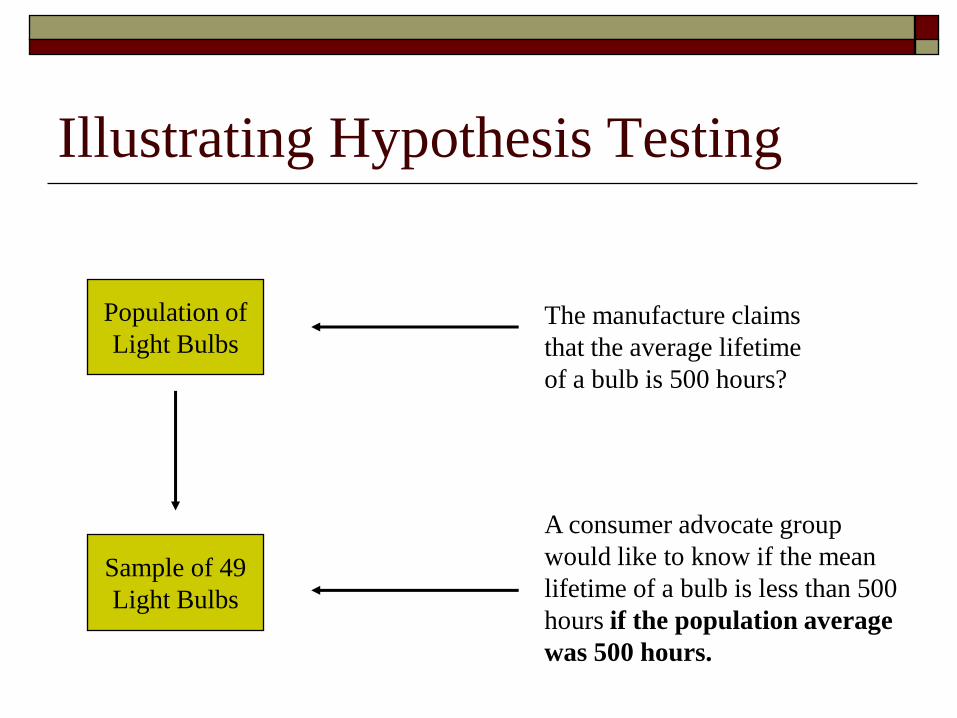
Illustrating Hypothesis Testing
Population of
Light Bulbs
Sample of 49
Light Bulbs
The manufacture claims
that the average lifetime
of a bulb is 500 hours?
A consumer advocate group
would like to know if the mean
lifetime of a bulb is less than 500
hours if the population average
was 500 hours.
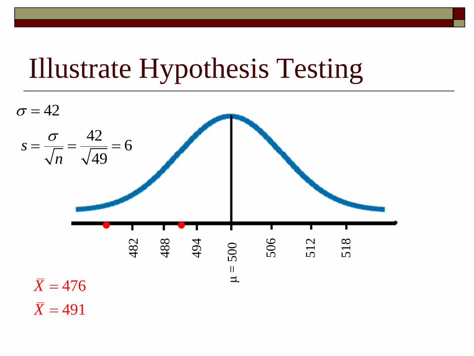
Illustrate Hypothesis Testing
426
49 s
n
μ=
50
0
49
4
48
8
48
2
51
8
51
2
50
6
42
476
491
X
X
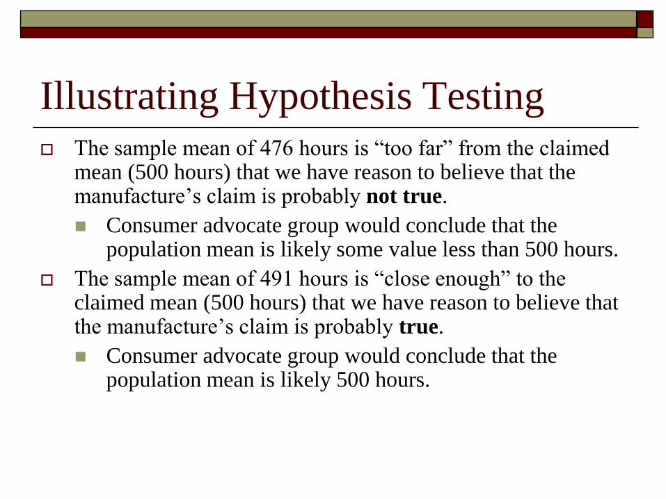
Illustrating Hypothesis Testing The sample mean of 476 hours is “too far” from the claimed
mean (500 hours) that we have reason to believe that the manufacture’s claim is probably not true.
Consumer advocate group would conclude that the population mean is likely some value less than 500 hours.
The sample mean of 491 hours is “close enough” to the claimed mean (500 hours) that we have reason to believe that the manufacture’s claim is probably true.
Consumer advocate group would conclude that the population mean is likely 500 hours.
Illustrating Hypothesis Testing
This raises an interesting question. How far
from the presumed mean of 500 hours can our
sample man be before we reject the idea that
the bulb lasts 500 hours?
To answer this question requires hypothesis
testing.
Definitions
In statistics, a hypothesis is a claim or
statement about a characteristic of a
population.
A hypothesis test (or test of significance) is
standard procedure for testing a claim about a
characteristic of a population.
The claims that we test regard the population
mean, population proportion and population
standard deviations.
Rare Event Rule for Inferential
Statistics If, under a given assumption, the probability
of a particular observed event is exceptionally
small, we conclude that the assumption if
probably not correct.
Example – Page 385, #2
What do you conclude? Use the rare event rule (Under a given assumption, the
probability of a particular observed event is exceptionally small, we conclude that
the assumption is probability not correct.
Claim: A gender selection method is effective in helping couples
have baby girls and among 50 babies, 49 are girls.
Gender selection appears to be effective. There is sufficient
evidence to support the claim. Under the assumption that the claim
is not true, having 49 girls among 50 babies would be a
rare event (unusual).
Two Types of Hypotheses
Null Hypothesis Ho
Includes the assumed value of the population parameter
Is the statement to be tested.
It is assume true until evidence we have indicated otherwise
Alternative Hypothesis H1 or Ha
The statement that the parameter has a value that somehow differs from the null hypothesis.
Is the claim to be tested.

Criminal Trial Analogy
First, State the 2 hypothesis
H0: Defendant is not guilty
H1: Defendant is guilty.
Then, collect evidence such finger prints, blood spots, hair samples, etc.
In statistics, the data is the evidence
Then, make initial assumption.
Defendant is innocent until proven guilty.
In statistics, we always assume the null hypothesis is true.
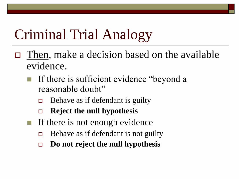
Criminal Trial Analogy
Then, make a decision based on the available evidence.
If there is sufficient evidence “beyond a reasonable doubt”
Behave as if defendant is guilty
Reject the null hypothesis
If there is not enough evidence
Behave as if defendant is not guilty
Do not reject the null hypothesis

Important Points
Neither decision entails proving the null
hypothesis or the alternative hypothesis.
We merely state there is enough evidence to
behave one way or the other.
This is also always true in statistics! No
matter what decision we make, there is
always a chance we made an error.
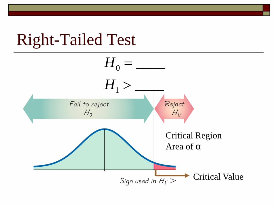
Right-Tailed Test
0
1
____
____
H
H
Critical Region
Area of α
Critical Value
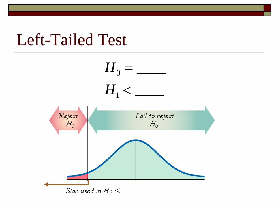
Left-Tailed Test
0
1
____
____
H
H
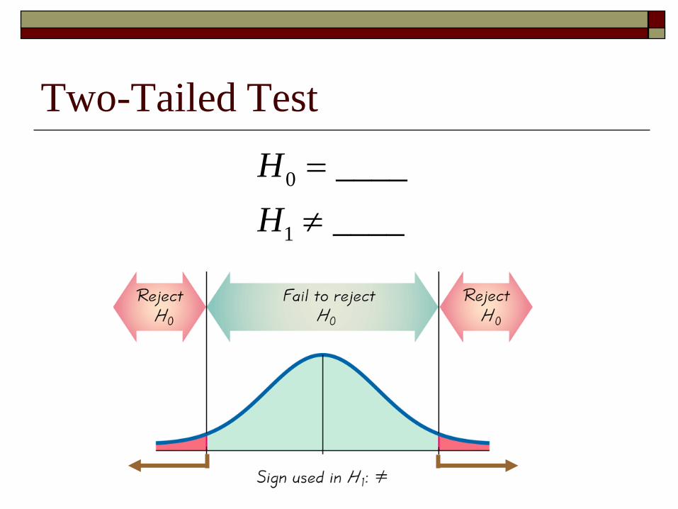
Two-Tailed Test
0
1
____
____
H
H

Example – Page 386, #6
Examine the given statements, than express the null hypothesis and alternative
hypothesis in symbolic form. Be sure to use the correct symbol (μ, σ, p) for
the indicated parameter.
The mean IQ of statistic students is at least 110.
0 : 110H
1 : 110H
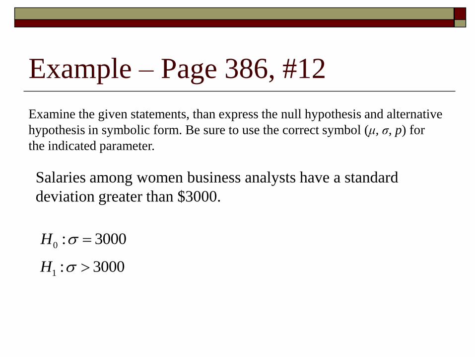
Example – Page 386, #12
Examine the given statements, than express the null hypothesis and alternative
hypothesis in symbolic form. Be sure to use the correct symbol (μ, σ, p) for
the indicated parameter.
Salaries among women business analysts have a standard
deviation greater than $3000.
0 : 3000H
1 : 3000H
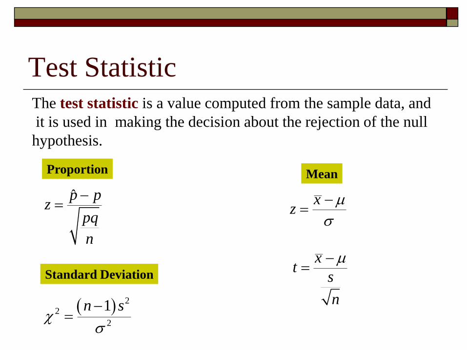
Test StatisticThe test statistic is a value computed from the sample data, and
it is used in making the decision about the rejection of the null
hypothesis.
Proportion Mean
Standard Deviation
p̂ pz
pq
n
2
2
2
1n s
xz
xt
s
n

Example – Page 387, #24
Find the test statistics. The claim is that the proportion of drivers stopped by
police in a year is different from the 10.3% reported by the Department of
Justice. Sample statistics include n = 800 randomly selected drivers with
12% of them stopped in the past year.
p̂ pz
pq
n
0.103
800
0.12ˆ
p
n
p
0.12 0.1031.5819 1.58
0.103 0.897
800
Definitions
The critical region or rejection region is the set of all values
of the test statistics that cause us to reject the null hypothesis.
The significance level () is the probability that the test
statistic will fall in the critical region when the null hypothesis
is actually true.
If the test statistic falls in the critical region, we reject the null hypothesis, so is the probability of making a mistake
of rejecting the null hypothesis when it is true.
Definitions
A critical value is any value that separates the
critical region (where reject the null
hypotheses) from the values of the test statistics
that do not lead to rejection of the null
hypothesis.
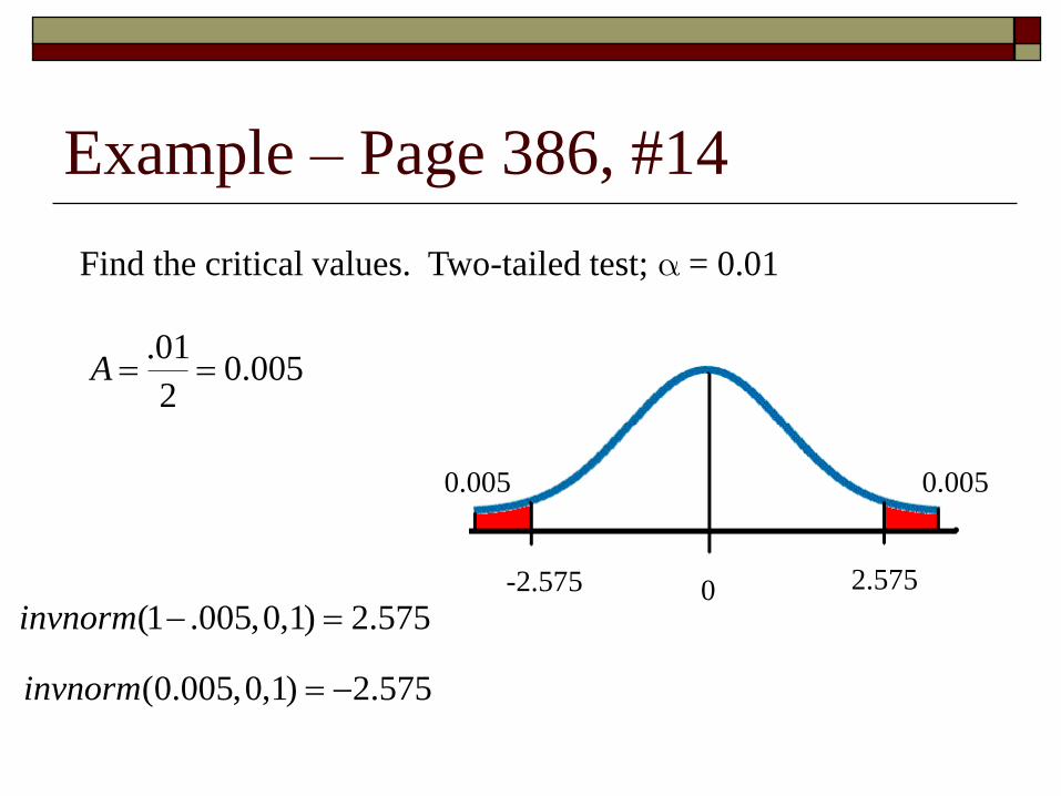
Example – Page 386, #14
Find the critical values. Two-tailed test; = 0.01
0
0.0050.005
(1 .005,0,1) 2.575invnorm
2.575
(0.005,0,1) 2.575invnorm
-2.575
.010.005
2A
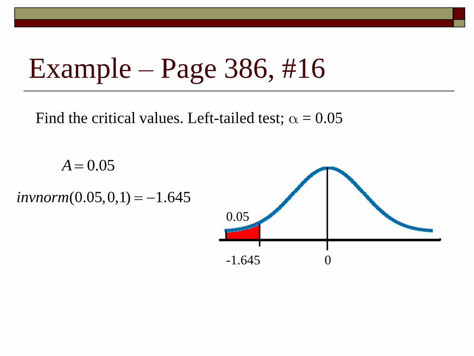
Example – Page 386, #16
Find the critical values. Left-tailed test; = 0.05
0
0.05
(0.05,0,1) 1.645invnorm
-1.645
0.05A
P-Values or Probability Values
The p-value is the probability of getting a value of the test statistic that is at least as extreme as the one representing the sample data, assuming that the null hypothesis is true.
The p-value represents how likely we would be to observe such an extreme sample if the null hypothesis were true.
If the p-value is “small” (Typically less than 0.05), we reject the null hypothesis.
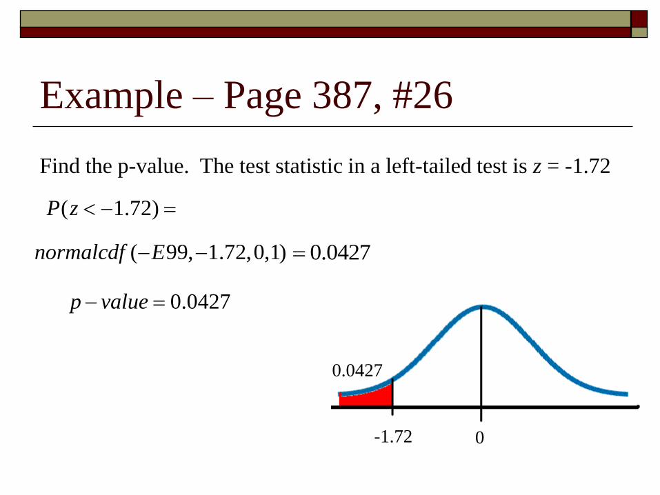
Example – Page 387, #26
Find the p-value. The test statistic in a left-tailed test is z = -1.72
0-1.72
( 1.72)P z
( 99, 1.72,0,1)normalcdf E 0.0427
0.0427
0.0427p value
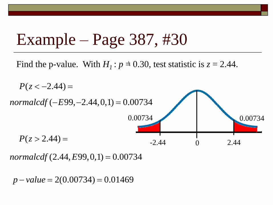
Example – Page 387, #30
Find the p-value. With H1 : p = 0.30, test statistic is z = 2.44.
0-2.44
( 2.44)P z
( 99, 2.44,0,1) 0.00734normalcdf E
2.44( 2.44)P z
(2.44, 99,0,1) 0.00734normalcdf E
2(0.00734) 0.01469p value
0.007340.00734
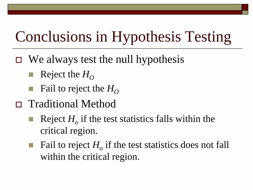
Conclusions in Hypothesis Testing
We always test the null hypothesis
Reject the HO
Fail to reject the HO
Traditional Method
Reject Ho if the test statistics falls within the
critical region.
Fail to reject Ho if the test statistics does not fall
within the critical region.

Conclusions in Hypothesis Testing
P-value Method
Reject the HO if P-value α (where α is the
significance level, such as 0.05).
Fail to reject the HO if P-value > α
Confidence Intervals
Because the confidence interval estimate of a
population parameter contains the likely values of
that parameter, reject a claim that the population
parameter has value that is not included in the
confidence interval.

Example – Page 387, #34
State the conclusion. Original claim: The proportion of college graduates who
smoke is less than 0.27. Initial conclusions: Reject the null hypothesis
There is sufficient evidence to support the claim that the
proportion of college graduates who smoke is less than 0.27.
: 0.27
: 0.27
o
a
H p
H p
Reject H0
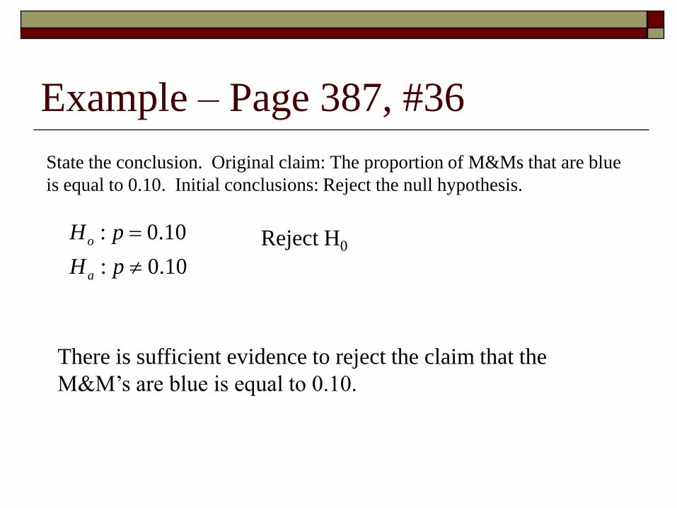
Example – Page 387, #36
State the conclusion. Original claim: The proportion of M&Ms that are blue
is equal to 0.10. Initial conclusions: Reject the null hypothesis.
There is sufficient evidence to reject the claim that the
M&M’s are blue is equal to 0.10.
: 0.10
: 0.10
o
a
H p
H p
Reject H0

Type I and Type II Errors
A Type I error is the mistake of rejecting the
null hypothesis when it is true.
The symbol α (alpha) is used to represent the
probability of making a type I error.
A Type II error is the mistake of failing to
reject the null hypothesis when it is false.
The symbol β (beta) is used to represent the
probability of a type II error
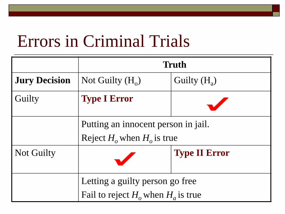
Errors in Criminal Trials
Truth
Jury Decision Not Guilty (Ho) Guilty (Ha)
Guilty Type I Error
Putting an innocent person in jail.
Reject Ho when Ho is true
Not Guilty Type II Error
Letting a guilty person go free
Fail to reject Ho when Ha is true
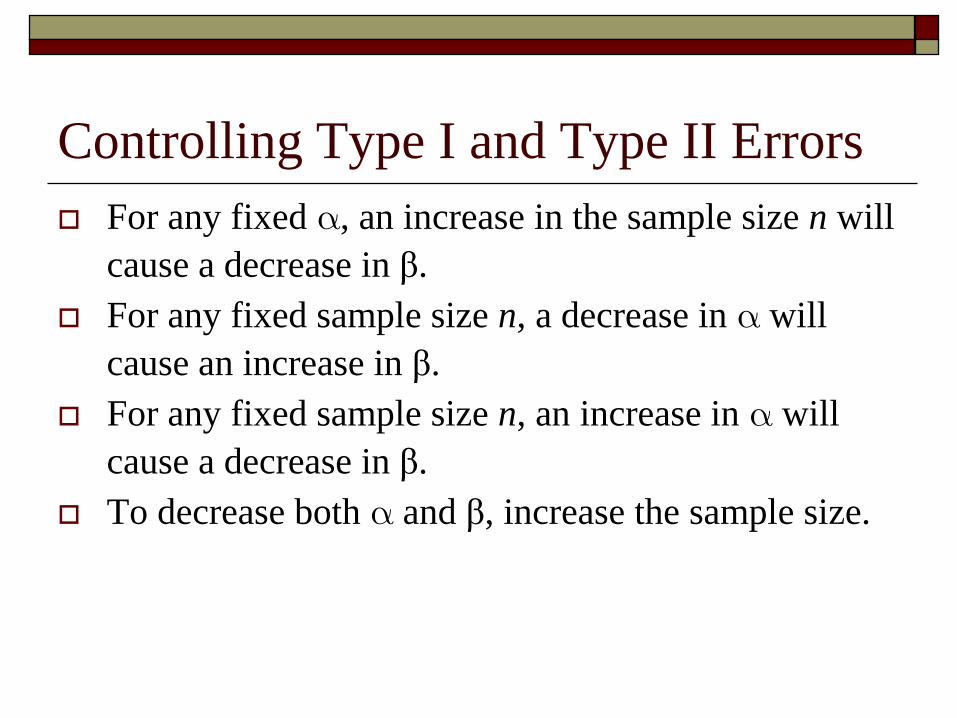
Controlling Type I and Type II Errors
For any fixed , an increase in the sample size n will
cause a decrease in β.
For any fixed sample size n, a decrease in will
cause an increase in β.
For any fixed sample size n, an increase in will
cause a decrease in β.
To decrease both and β, increase the sample size.
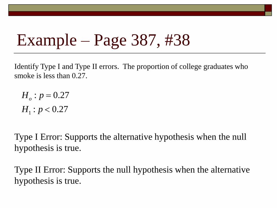
Example – Page 387, #38
Identify Type I and Type II errors. The proportion of college graduates who
smoke is less than 0.27.
1
: 0.27
: 0.27
oH p
H p
Type I Error: Supports the alternative hypothesis when the null
hypothesis is true.
Type II Error: Supports the null hypothesis when the alternative
hypothesis is true.

Lesson 7-3
Testing a Claim about a Proportion
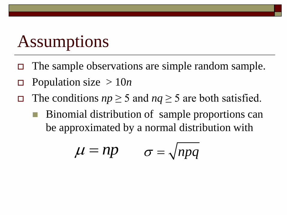
Assumptions
The sample observations are simple random sample.
Population size > 10n
The conditions np ≥ 5 and nq ≥ 5 are both satisfied.
Binomial distribution of sample proportions can
be approximated by a normal distribution with
np npq

Test Statistic
n = sample size of number of trials
p = population proportion
(used in the null hypothesis)
ˆx
pn
1q p
p̂ pz
pq
n
sample proportion
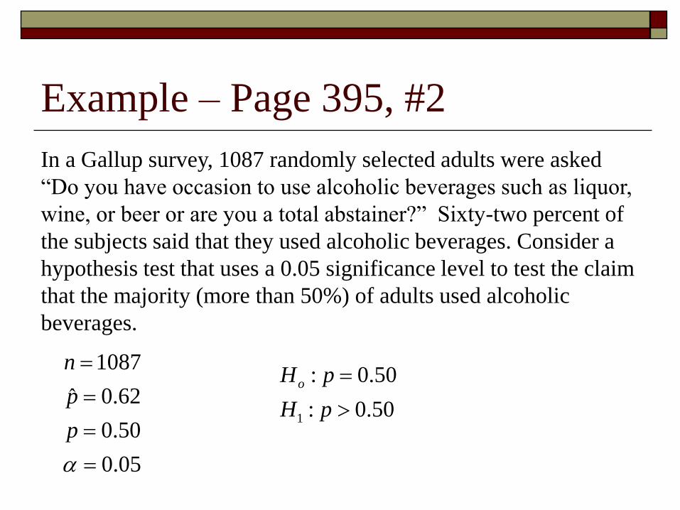
Example – Page 395, #2
In a Gallup survey, 1087 randomly selected adults were asked
“Do you have occasion to use alcoholic beverages such as liquor,
wine, or beer or are you a total abstainer?” Sixty-two percent of
the subjects said that they used alcoholic beverages. Consider a
hypothesis test that uses a 0.05 significance level to test the claim
that the majority (more than 50%) of adults used alcoholic
beverages.
1087
0.62ˆ
0.50
0.05
n
p
p
1
: 0.50
: 0.50
oH p
H p
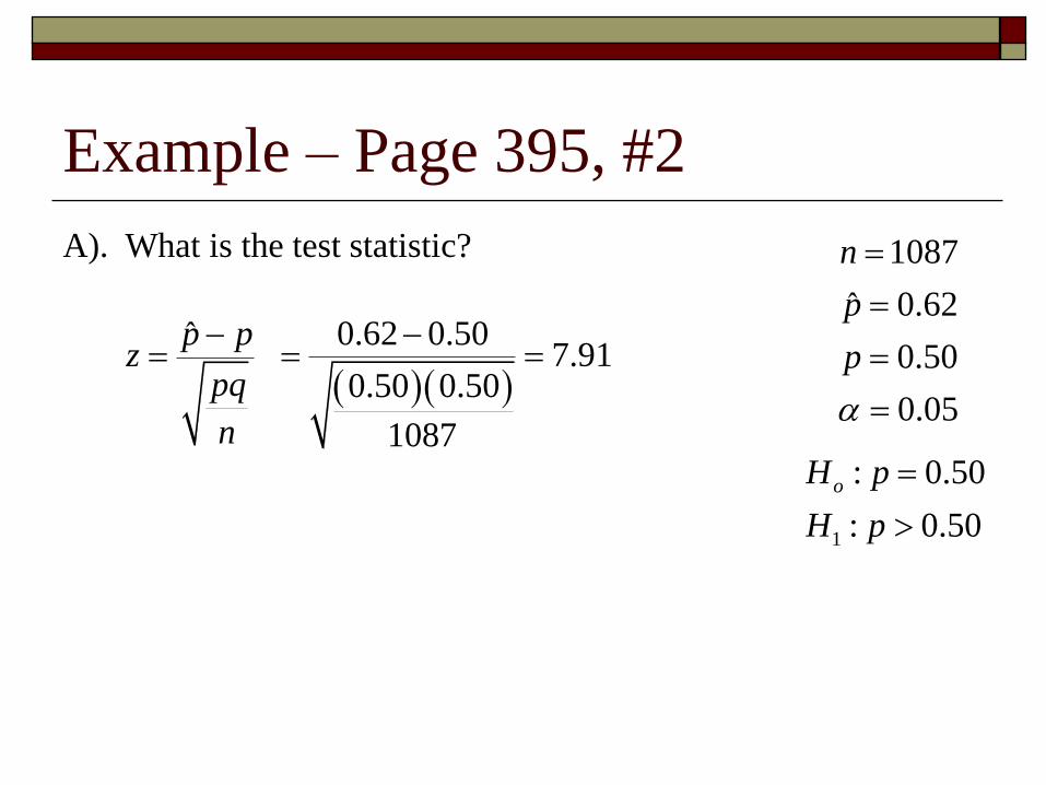
Example – Page 395, #2
A). What is the test statistic? 1087
0.62ˆ
0.50
0.05
n
p
p
1
: 0.50
: 0.50
oH p
H p
p̂ pz
pq
n
0.62 0.507.91
0.50 0.50
1087

Example – Page 395, #2
1087
0.62ˆ
0.50
0.05
n
p
p
1
: 0.50
: 0.50
oH p
H p
B). What is the critical value?
ˆ7.91pz
0.05
(1 .05,0,1) 1.645invnorm
1.645 7.91
Example – Page 395, #2
1087
0.62ˆ
0.50
0.05
n
p
p
1
: 0.50
: 0.50
oH p
H p
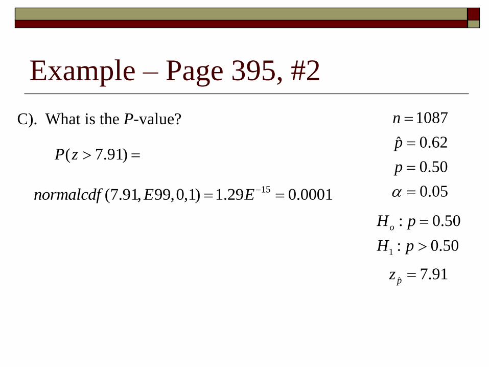
C). What is the P-value?
ˆ7.91pz
15(7.91, 99,0,1) 1.29 0.0001normalcdf E E
( 7.91)P z
Example – Page 395, #2
1
: 0.50
: 0.50
oH p
H p
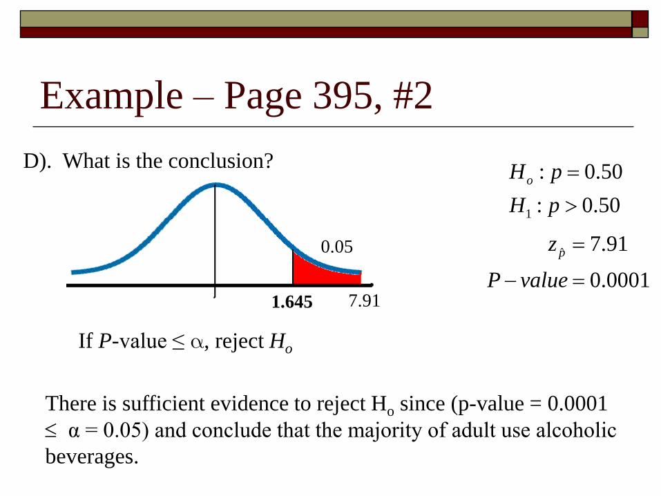
D). What is the conclusion?
ˆ7.91
0.0001
pz
P value
0.05
1.645 7.91
If P-value ≤ , reject Ho
There is sufficient evidence to reject Ho since (p-value = 0.0001
α = 0.05) and conclude that the majority of adult use alcoholic
beverages.
Example – Page 395, #2
E). Based on the preceding results, can we conclude that 62% is
significantly greater than 50% for all such hypothesis tests?
No, 62% might not be significantly greater than 50% for some
samples, such as one with n = 50

Example – Page 395, #2
Stats/Tests/5:1-PropZTest
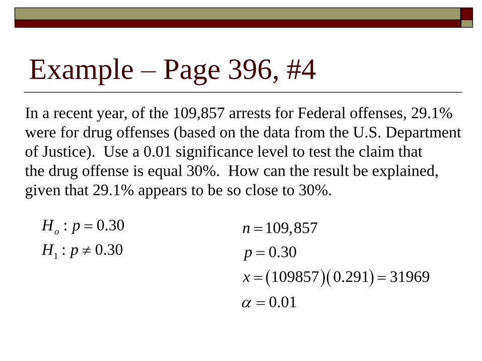
Example – Page 396, #4
In a recent year, of the 109,857 arrests for Federal offenses, 29.1%
were for drug offenses (based on the data from the U.S. Department
of Justice). Use a 0.01 significance level to test the claim that
the drug offense is equal 30%. How can the result be explained,
given that 29.1% appears to be so close to 30%.
1
: 0.30
: 0.30
oH p
H p
109,857
0.30
109857 0.291 31969
0.01
n
p
x
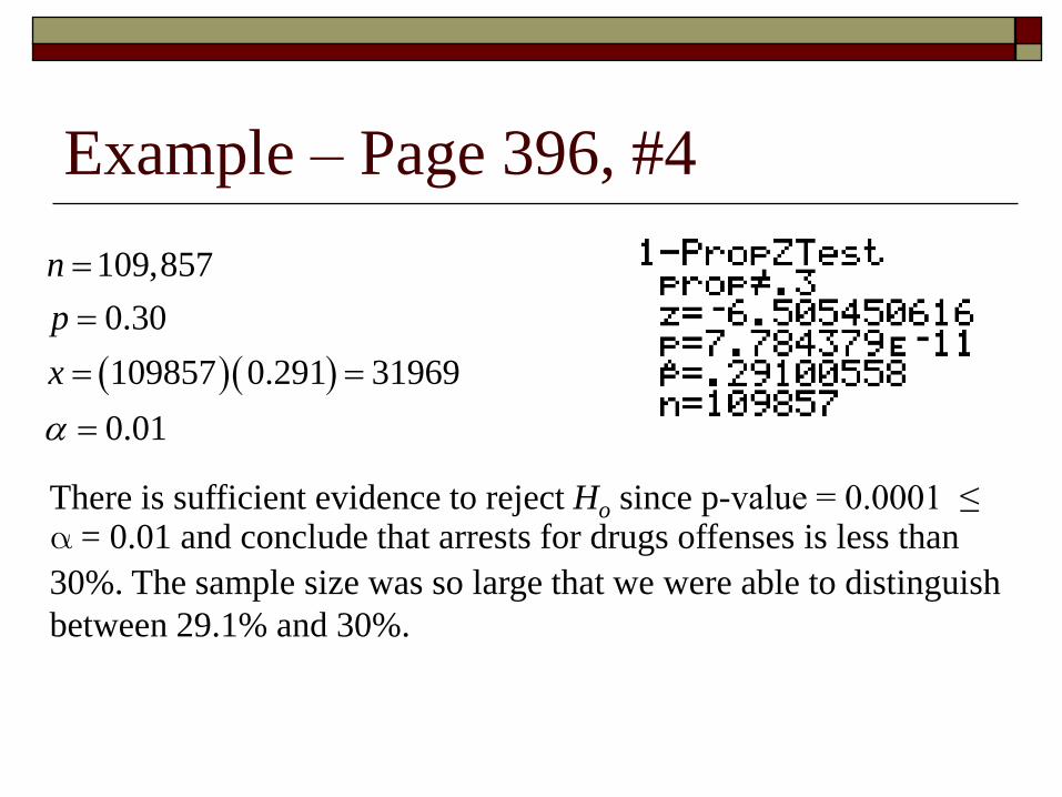
Example – Page 396, #4
109,857
0.30
109857 0.291 31969
0.01
n
p
x
There is sufficient evidence to reject Ho since p-value = 0.0001 ≤ = 0.01 and conclude that arrests for drugs offenses is less than
30%. The sample size was so large that we were able to distinguish
between 29.1% and 30%.
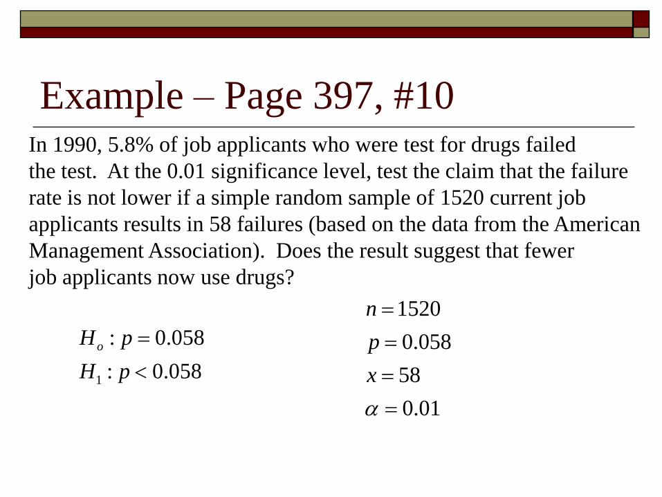
Example – Page 397, #10In 1990, 5.8% of job applicants who were test for drugs failed
the test. At the 0.01 significance level, test the claim that the failure
rate is not lower if a simple random sample of 1520 current job
applicants results in 58 failures (based on the data from the American
Management Association). Does the result suggest that fewer
job applicants now use drugs?
1520
0.058
58
0.01
n
p
x
1
: 0.058
: 0.058
oH p
H p
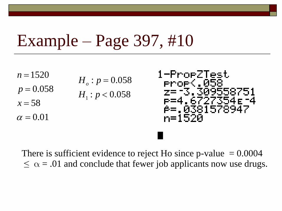
Example – Page 397, #10
1520
0.058
58
0.01
n
p
x
1
: 0.058
: 0.058
oH p
H p
There is sufficient evidence to reject Ho since p-value = 0.0004≤ = .01 and conclude that fewer job applicants now use drugs.

Example – Page 397, #16A simple random sample of households with TV sets in use show that 1024 of
them were tuned to 60 Minutes while 3836 were tuned to some other show. Use a
0.025 significance level to test the claim of a CBS executive that “60 Minutes gets
more than a 20 share,” which means that more than 20% of the sets in use are
turned to 60 Minutes. If you are a commercial advertiser and you are trying to
negotiate lower costs, what would you argue?
4860
1024
0.20
0.025
n
x
p
1
: 0.20
: 0.20
oH p
H p
p = proportion of households that were tuned to 60 Minutes.
Step 1 – Identify the population of interest and the parameter you want to draw
conclusions about.

Example – Page 397, #16
4860
1024
0.20
0.025
n
x
p
1
: 0.20
: 0.20
oH p
H p
Use a one proportion z-test
Question stated SRS
Population size > 10(4860) = 48600
np = (4860)(0.20) = 972 ≥ 5
and nq = (4860)(.80) = 3888 ≥ 5
Step 2 – Choose the appropriate inference procedure. Verify
conditions for using the selected procedure.
Example – Page 397, #16
4860
1024
0.20
0.025
n
x
p
1
: 0.20
: 0.20
oH p
H p
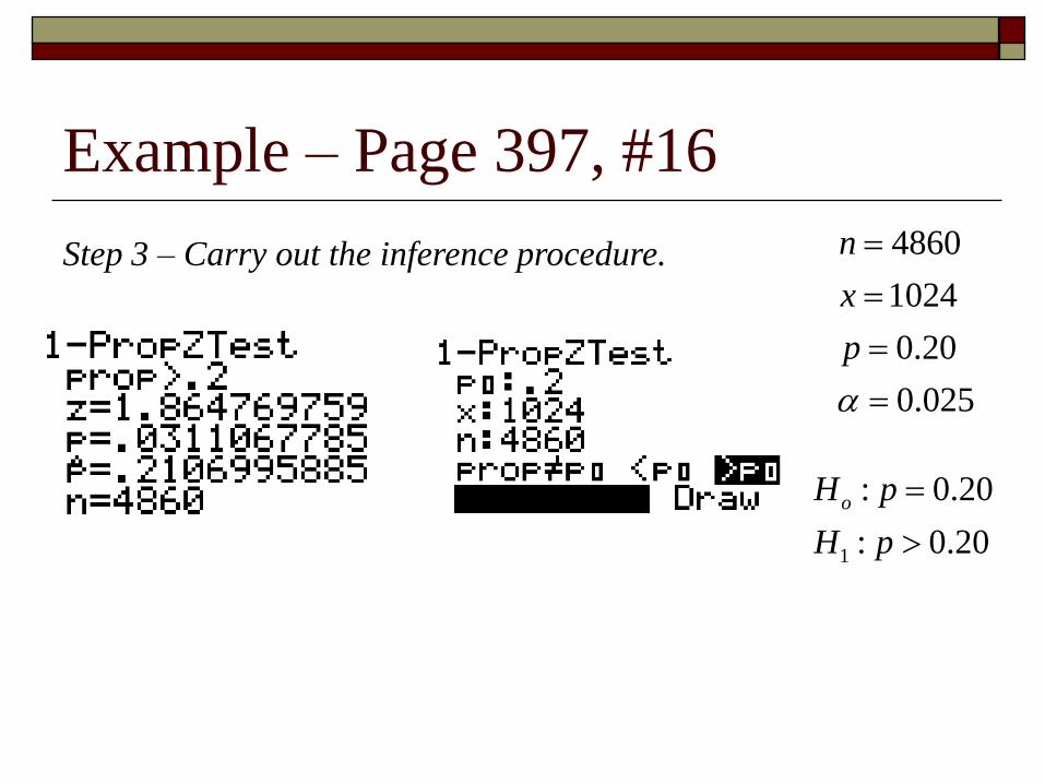
Step 3 – Carry out the inference procedure.
Example – Page 397, #16
4860
1024
0.20
0.025
n
x
p
1
: 0.20
: 0.20
oH p
H p
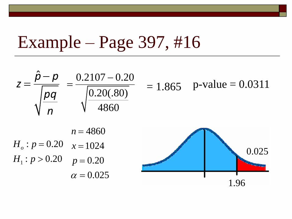
p̂ pz
pq
n
0.025
0.2107 0.20
0.20(.80)
4860
= 1.865 p-value = 0.0311
1.96
Example – Page 397, #16
There is sufficient evidence to fail to reject Ho since P-value = 0.0311 > = 0.025 and are unable to conclude
that more than 20% of households are watching 60
Minutes.
Even though happens to be greater than 20%,
that is not enough evidence to 97.5% (1 – 0.025 = 0.975)
certain that the true population proportion is greater
than 20%.
0.211p̂
Step 4 – Interpret your results in the context of the problem.
Lesson 7-4
Testing a Claim About a Mean: σ Known
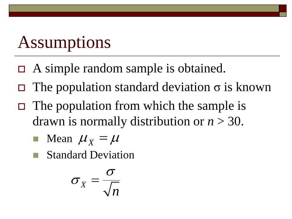
Assumptions
A simple random sample is obtained.
The population standard deviation σ is known
The population from which the sample is
drawn is normally distribution or n > 30.
Mean
Standard Deviation
X
Xn
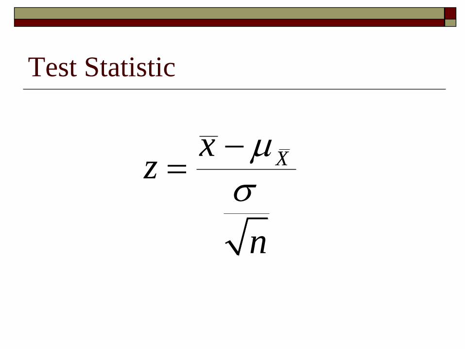
Test Statistic
Xxz
n
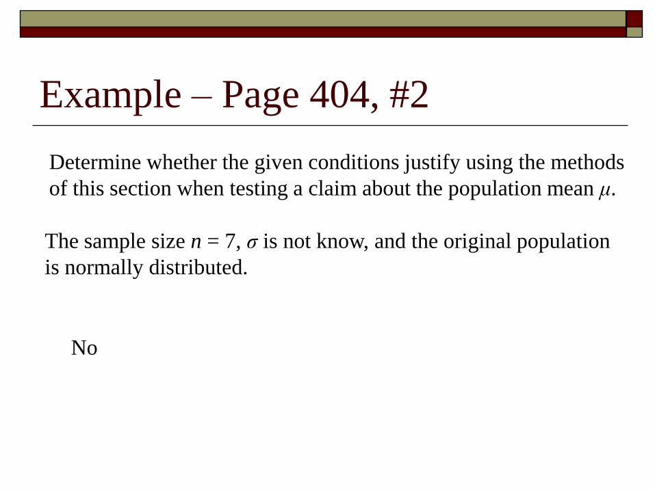
Example – Page 404, #2
Determine whether the given conditions justify using the methods
of this section when testing a claim about the population mean μ.
The sample size n = 7, σ is not know, and the original population
is normally distributed.
No
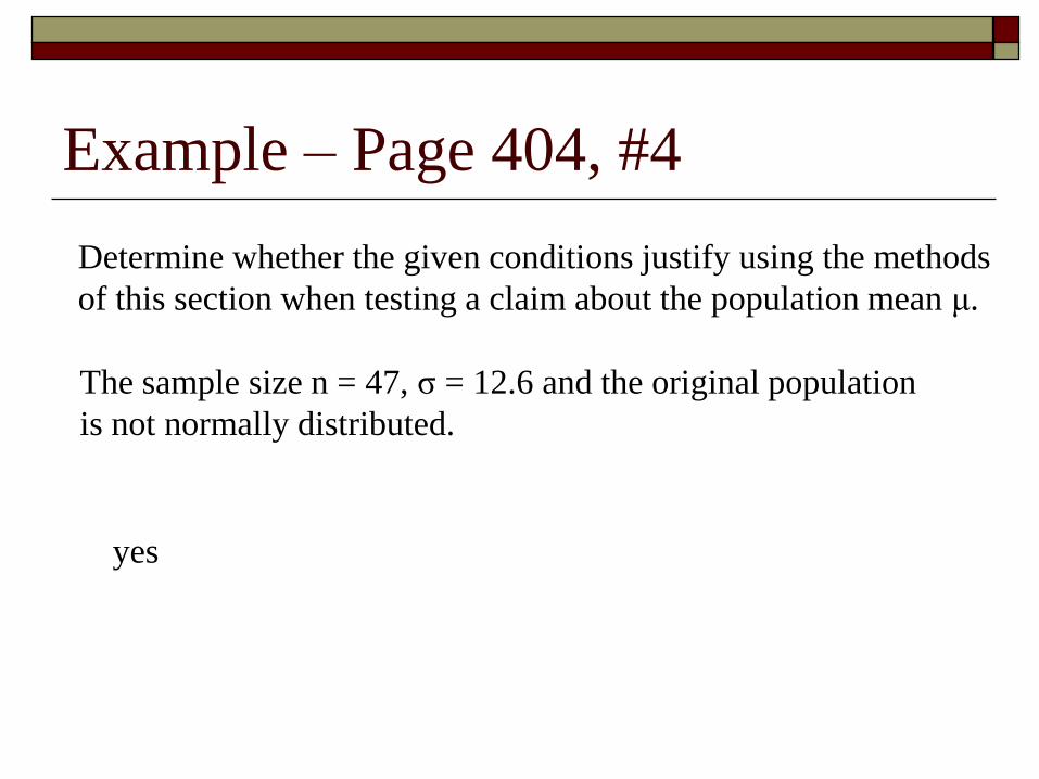
Example – Page 404, #4
Determine whether the given conditions justify using the methods
of this section when testing a claim about the population mean μ.
The sample size n = 47, σ = 12.6 and the original population
is not normally distributed.
yes
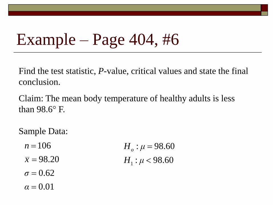
Example – Page 404, #6
Find the test statistic, P-value, critical values and state the final
conclusion.
Claim: The mean body temperature of healthy adults is less
than 98.6° F.
Sample Data:
106
98.20
0.62
0.01
n
x
σ
α
1
: 98.60
: 98.60
oH μ
H μ
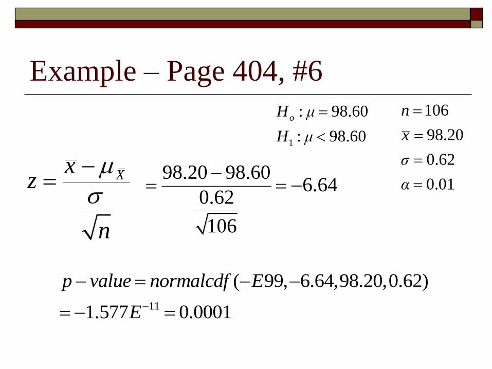
Example – Page 404, #6
106
98.20
0.62
0.01
n
x
σ
α
1
: 98.60
: 98.60
oH μ
H μ
Xxz
n
98.20 98.60
6.640.62
106
11
( 99, 6.64,98.20,0.62)
1.577 0.0001
p value normalcdf E
E

Example – Page 404, #6
106
98.20
0.62
0.01
n
x
σ
α
1
: 98.60
: 98.60
oH μ
H μ
0.01
2.33
(0.01) 2.33invnorm
Critical Value
Example – Page 404, #6
Final Conclusion
Reject Ho since the P-value ≤ , there is sufficient evidence
to support the claim that the mean is less than 98.6°F.
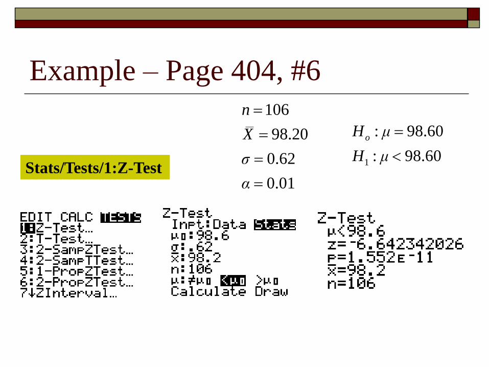
Example – Page 404, #6
106
98.20
0.62
0.01
n
X
σ
α
1
: 98.60
: 98.60
oH μ
H μ
Stats/Tests/1:Z-Test
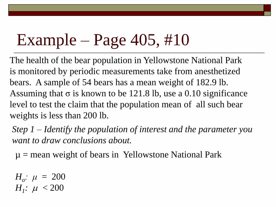
Example – Page 405, #10The health of the bear population in Yellowstone National Park
is monitored by periodic measurements take from anesthetized
bears. A sample of 54 bears has a mean weight of 182.9 lb.
Assuming that σ is known to be 121.8 lb, use a 0.10 significance
level to test the claim that the population mean of all such bear
weights is less than 200 lb.
µ = mean weight of bears in Yellowstone National Park
Ho: μ = 200
H1: < 200
Step 1 – Identify the population of interest and the parameter you
want to draw conclusions about.
Example – Page 405, #10
Use a one sample z-test
Not sure if it’s a SRS – should be representative the population.
Standard deviation of the population is known
Approximately normal distributed since n > 30
Step 2 – Choose the appropriate inference procedure. Verify the
conditions for using the selected procedure.
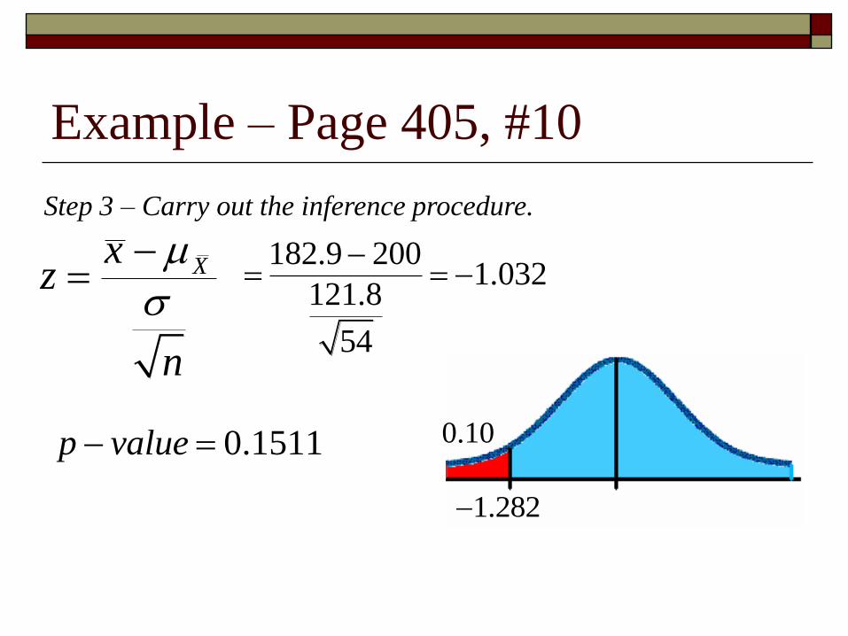
Example – Page 405, #10
Xxz
n
0.10
1.282
182.9 2001.032
121.8
54
0.1511p value
Step 3 – Carry out the inference procedure.
Example – Page 405, #10
There is sufficient evidence to fail to reject Ho since (p-value =
0.151 > α = 0.10) and are unable to conclude that weight of
bears in Yellowstone National Park is less than 200 lbs.
Step 4 – Interpret your results in the context of the problem
Underlying Rational of
Hypothesis Testing If the sample results can easily occur when
assumption (null hypothesis) is true, we attribute the
relatively small discrepancy between the assumption
and the sample results to chance.
If the sample results cannot easily occur when that
assumption (null hypothesis) is true, we explain the
relatively large discrepancy between the assumption
and the sample by concluding that the assumption is
not true.
Example – Page 406, #14
Analysis of the last digits of sample data values sometimes reveals
whether the data have been accurately measured and reported. When
single digits 0 through 9 are randomly selected with replacement,
the mean should be 4.50 and the standard deviation should be 2.87.
Reported data (such as weights or heights) are often rounded so
that the last digits include disproportionately more 0s and 5s. The
last digits in the reported lengths (in feet) of the 73 home runs hit
by Barry Bonds in 2001 are used to test the claim that they come from
a population with mean 4.50 (based on data from USA Today). When
Minitab is used to test the claim, the display is as shown here. Using
a 0.05 significance level, interpret the Minitab results. Does it
appear that the distances were accurately measured?
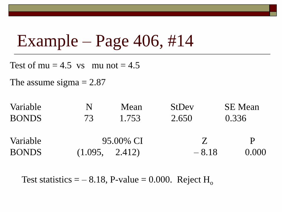
Example – Page 406, #14
Test of mu = 4.5 vs mu not = 4.5
The assume sigma = 2.87
Variable N Mean StDev SE Mean
BONDS 73 1.753 2.650 0.336
Variable 95.00% CI Z P
BONDS (1.095, 2.412) – 8.18 0.000
Test statistics = – 8.18, P-value = 0.000. Reject Ho
Lesson 7-5
Testing a Claim about a Mean: σ Not Known
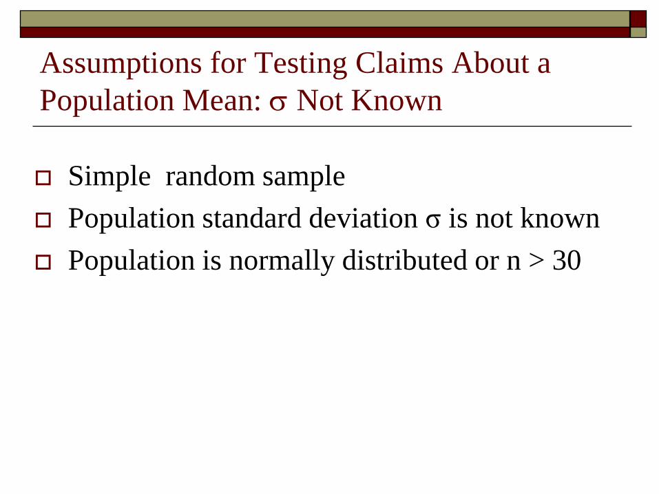
Assumptions for Testing Claims About a
Population Mean: Not Known
Simple random sample
Population standard deviation σ is not known
Population is normally distributed or n > 30
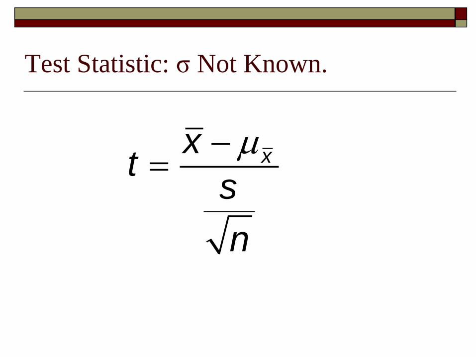
Test Statistic: σ Not Known.
xxt
s
n
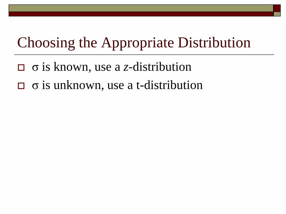
Choosing the Appropriate Distribution
σ is known, use a z-distribution
σ is unknown, use a t-distribution
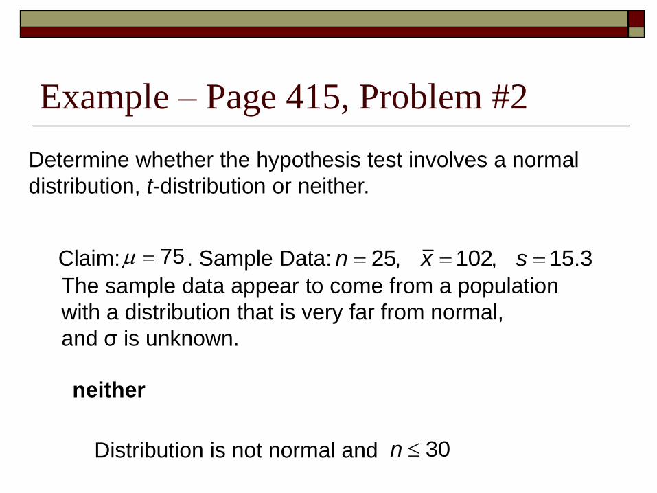
Example – Page 415, Problem #2
Claim: . Sample Data: 75 25, 102, 15.3n x s
Determine whether the hypothesis test involves a normal
distribution, t-distribution or neither.
The sample data appear to come from a population
with a distribution that is very far from normal,
and σ is unknown.
neither
Distribution is not normal and 30n
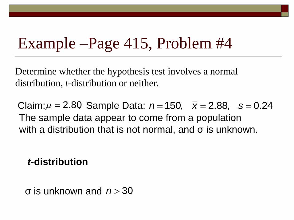
Example –Page 415, Problem #4
Claim: . Sample Data: 2.80 150, 2.88, 0.24n x s
Determine whether the hypothesis test involves a normal
distribution, t-distribution or neither.
The sample data appear to come from a population
with a distribution that is not normal, and σ is unknown.
t-distribution
σ is unknown and 30n

Example - Page 415, Problem #8
Two-Tailed test with and test statistic
Find the P-value.
9n 1.577t
Use Table A-3 8df
1.577 Falls between: 1.860 and 1.397
P-value is between: 0.10 and 0.20
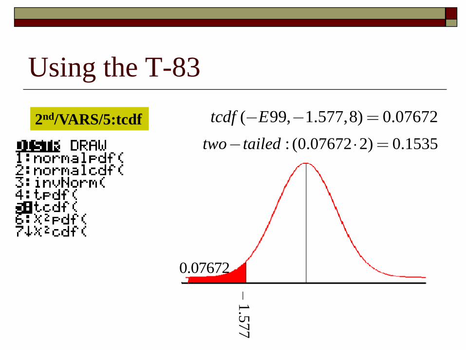
Using the T-83
2nd/VARS/5:tcdf ( 99, 1.577,8) 0.07672tcdf E
: (0.07672 2) 0.1535two tailed
0.07672
–1.5
77
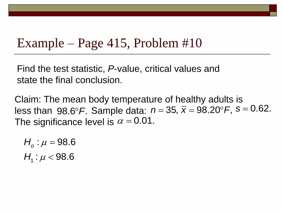
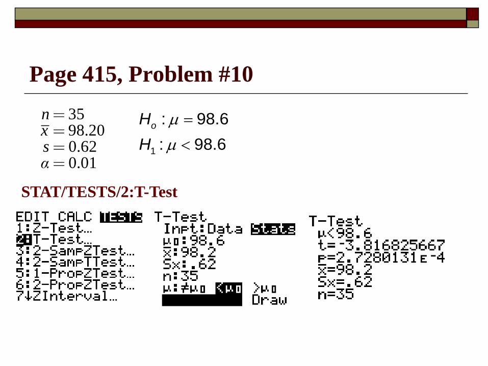
Example – Page 415, Problem #10
Find the test statistic, P-value, critical values and
state the final conclusion.
Claim: The mean body temperature of healthy adults is
less than Sample data:
The significance level is 98.6 .F 35,n 98.20 ,x F 0.62.s
0.01.
1
: 98.6
: 98.6
oH
H
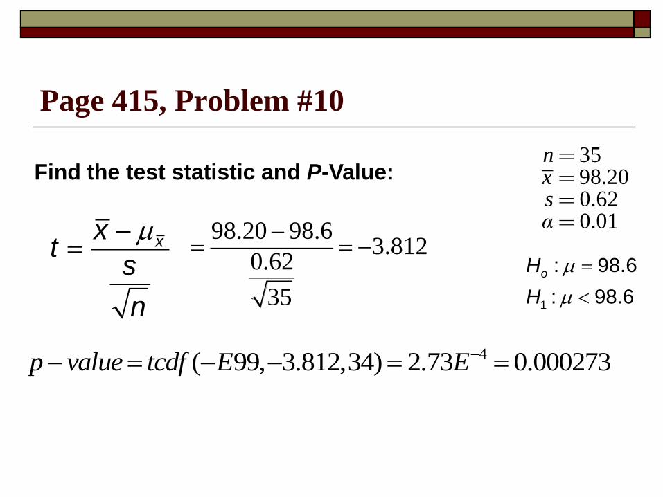
Page 415, Problem #10
1
: 98.6
: 98.6
oH
H
Find the test statistic and P-Value:3598.200.620.01
nxsα
xxt
s
n
98.20 98.63.812
0.62
35
4( 99, 3.812,34) 2.73 0.000273p value tcdf E E

Page 415, Problem #10
1
: 98.6
: 98.6
oH
H
Final Conclusion3598.200.620.01
nXsα
0.000273pv
Reject Ho since P-value ≤ α, there is
sufficient evidence to conclude that
μ < 98.6
Page 415, Problem #10
1
: 98.6
: 98.6
oH
H
3598.200.620.01
nxsα
STAT/TESTS/2:T-Test
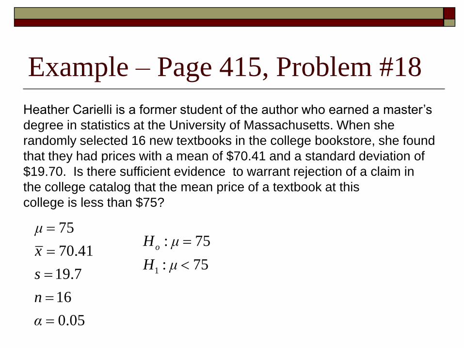
Example – Page 415, Problem #18
Heather Carielli is a former student of the author who earned a master’s
degree in statistics at the University of Massachusetts. When she
randomly selected 16 new textbooks in the college bookstore, she found
that they had prices with a mean of $70.41 and a standard deviation of
$19.70. Is there sufficient evidence to warrant rejection of a claim in
the college catalog that the mean price of a textbook at this
college is less than $75?
1
: 75
: 75
oH μ
H μ
75
70.41
19.7
16
0.05
μ
x
s
n
α
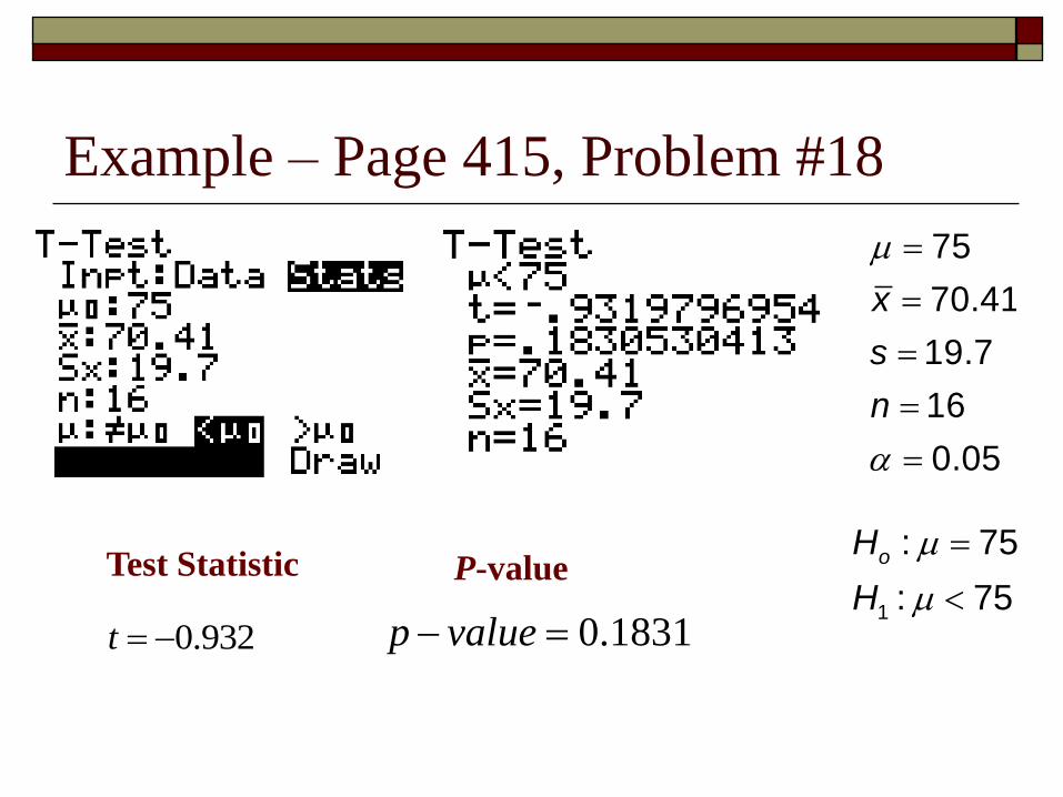
Example – Page 415, Problem #18
1
: 75
: 75
oH
H
75
70.41
19.7
16
0.05
x
s
n
0.932 t 0.1831 p value
Test Statistic P-value
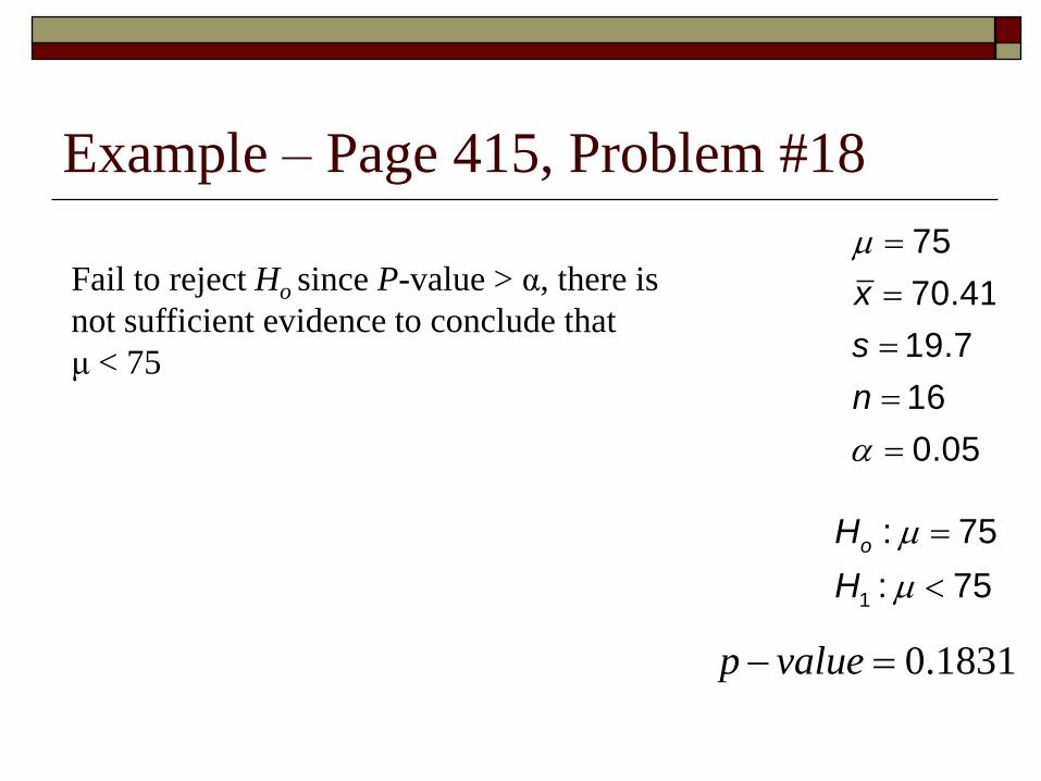
Example – Page 415, Problem #18
1
: 75
: 75
oH
H
75
70.41
19.7
16
0.05
x
s
n
0.1831 p value
Fail to reject Ho since P-value > α, there is
not sufficient evidence to conclude that
μ < 75
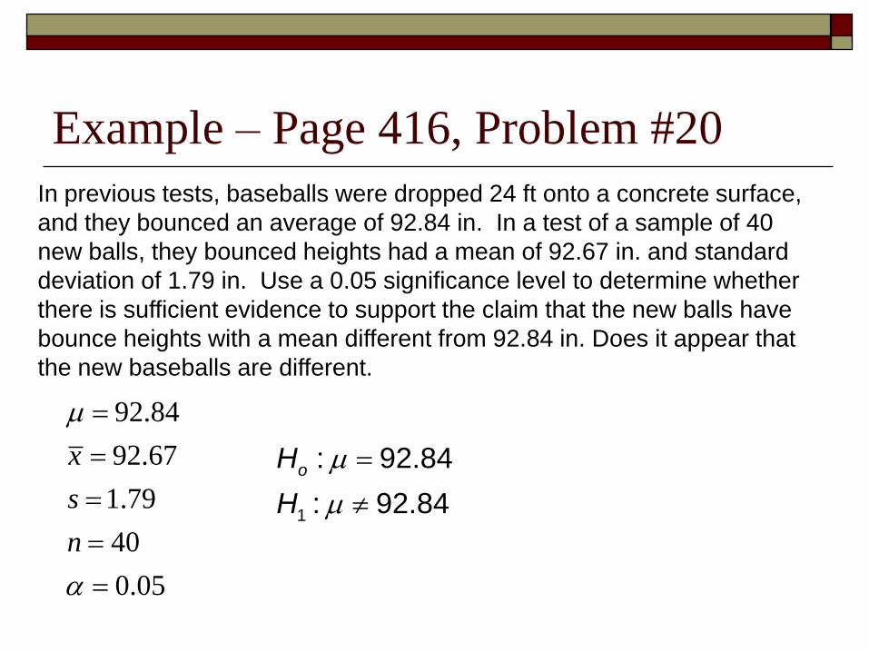
Example – Page 416, Problem #20
In previous tests, baseballs were dropped 24 ft onto a concrete surface,
and they bounced an average of 92.84 in. In a test of a sample of 40
new balls, they bounced heights had a mean of 92.67 in. and standard
deviation of 1.79 in. Use a 0.05 significance level to determine whether
there is sufficient evidence to support the claim that the new balls have
bounce heights with a mean different from 92.84 in. Does it appear that
the new baseballs are different.
1
: 92.84
: 92.84
oH
H
92.84
92.67
1.79
40
0.05
x
s
n
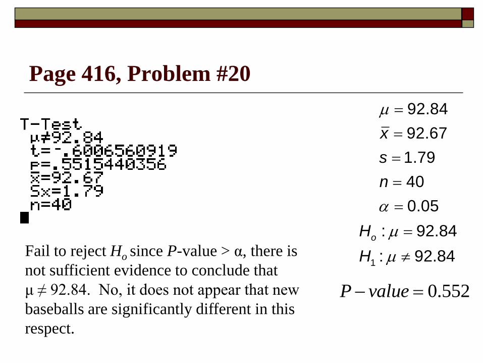
Page 416, Problem #20
1
: 92.84
: 92.84
oH
H
92.84
92.67
1.79
40
0.05
x
s
n
Fail to reject Ho since P-value > α, there is
not sufficient evidence to conclude that
μ ≠ 92.84. No, it does not appear that new
baseballs are significantly different in this
respect.
0.552P value
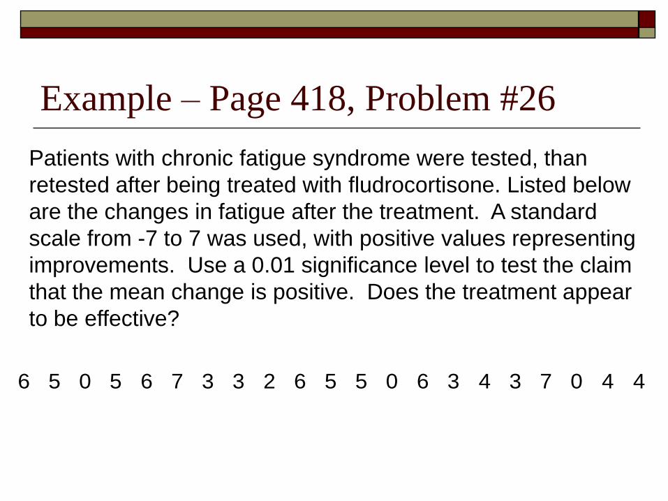
Example – Page 418, Problem #26
Patients with chronic fatigue syndrome were tested, than
retested after being treated with fludrocortisone. Listed below
are the changes in fatigue after the treatment. A standard
scale from -7 to 7 was used, with positive values representing
improvements. Use a 0.01 significance level to test the claim
that the mean change is positive. Does the treatment appear
to be effective?
6 5 0 5 6 7 3 3 2 6 5 5 0 6 3 4 3 7 0 4 4
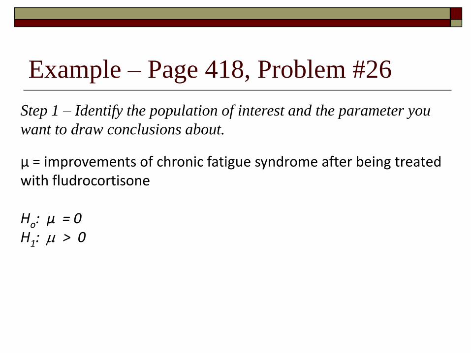
Example – Page 418, Problem #26
µ = improvements of chronic fatigue syndrome after being treated with fludrocortisone
Ho: μ = 0 H1: > 0
Step 1 – Identify the population of interest and the parameter you
want to draw conclusions about.
Example – Page 418, Problem #26
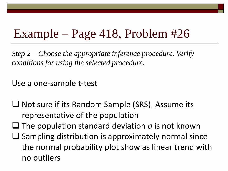
Use a one-sample t-test
Not sure if its Random Sample (SRS). Assume itsrepresentative of the population
The population standard deviation σ is not known Sampling distribution is approximately normal since
the normal probability plot show as linear trend withno outliers
Step 2 – Choose the appropriate inference procedure. Verify
conditions for using the selected procedure.
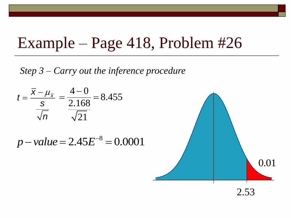
Example – Page 418, Problem #26
xx
ts
n
0.01
2.53
4 08.455
2.168
21
82.45 0.0001p value E
Step 3 – Carry out the inference procedure
Example – Page 418, Problem #26
There is sufficient evidence to reject Ho since
(p-value = 0.0001 α = 0.01) and conclude that
there was improvements for patients with chronic
fatigue syndrome that was treated with
fludrocortisone.
Step 4 – Interpret your results in the context of the problem
Lesson 7-6
Testing a Claim about a Standard Deviation or
Variance
Main Idea of
Standard Deviation and Variance
The main idea is that the standard deviation
and the variance are measures of consistency.
The less consistent the values of a variable,
the higher the standard deviation of the
variable

Assumptions for Testing Claims
about σ and σ²
The sample is simple random
The population has a normal distribution.

Test Statistic for Testing Claim
about σ and σ²
22
2
( 1)n s
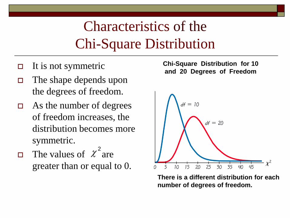
Characteristics of the
Chi-Square Distribution
It is not symmetric
The shape depends upon
the degrees of freedom.
As the number of degrees
of freedom increases, the
distribution becomes more
symmetric.
The values of are
greater than or equal to 0.There is a different distribution for each
number of degrees of freedom.
Chi-Square Distribution for 10
and 20 Degrees of Freedom
2
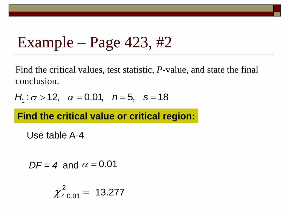
Example – Page 423, #2
Find the critical values, test statistic, P-value, and state the final
conclusion.
1 : 12, 0.01, 5, 18H n s
Find the critical value or critical region:
Use table A-4
DF = 4 and 0.01
2
4,0.01 13.277
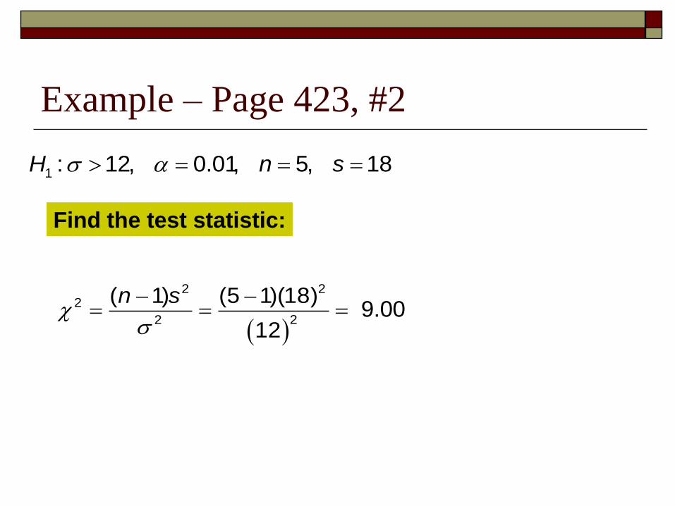
Example – Page 423, #2
1 : 12, 0.01, 5, 18H n s
Find the test statistic:
2 22
22
( 1) (5 1)(18)
12
n s
9.00

Example – Page 423, #2
1 : 12, 0.01, 5, 18H n s
Find the P-value:
Use Table A-4
4df and 9.00
0.05 0.10p value
Use TI-83
2 (9, 99,4)cdf E 0.0611
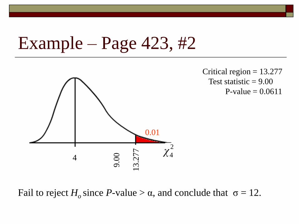
Example – Page 423, #2
Critical region = 13.277
Test statistic = 9.00
P-value = 0.0611
4
2
4χ
0.0113
.27
7
9.0
0
Fail to reject Ho since P-value > α, and conclude that σ = 12.

Example – Page 424, #4
Find the critical values, test statistic, P-value, and state the final
conclusion.
1 : 4, 0.05, 81, 4.7H n s
Find the critical value or critical region:
Use table A-4
DF = 80 and = 0.05
2 2
.025 106.629Rχ χ 2 2
.975 57.153Lχ χ
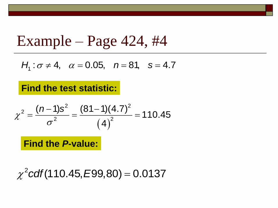
Example – Page 424, #4
2 22
22
( 1) (81 1)(4.7)110.45
4
n s
1 : 4, 0.05, 81, 4.7H n s
Find the test statistic:
Find the P-value:
2 (110.45, 99,80) 0.0137cdf E
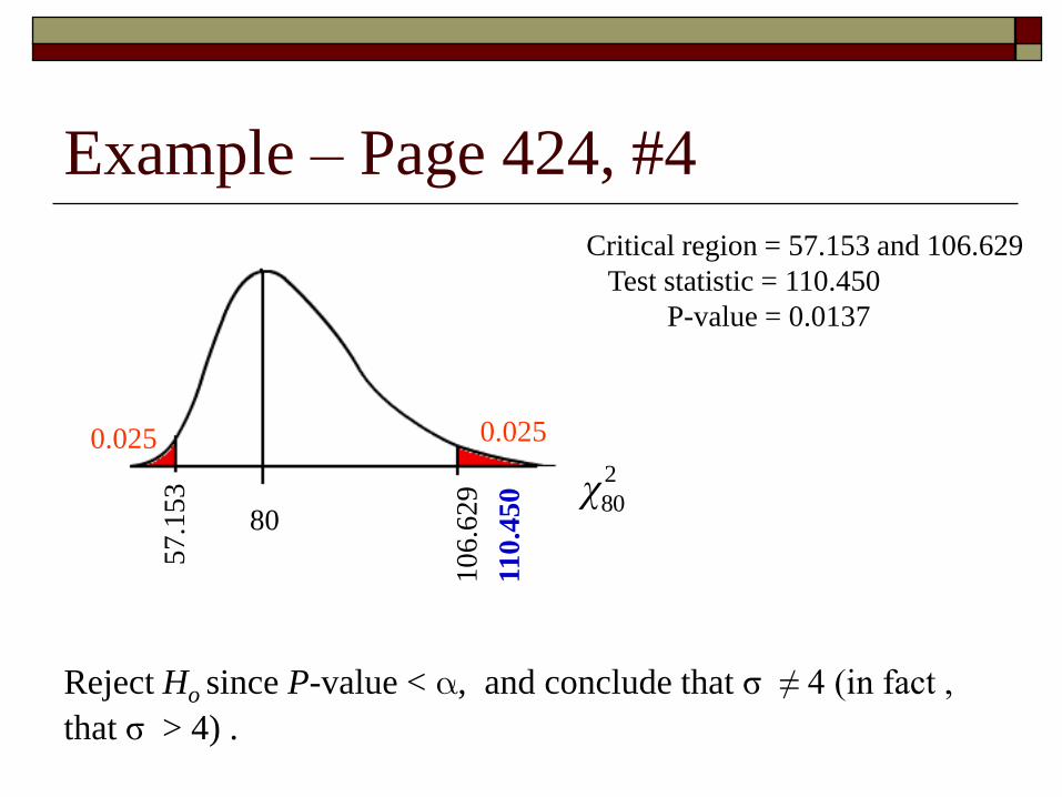
Example – Page 424, #4
Critical region = 57.153 and 106.629
Test statistic = 110.450
P-value = 0.0137
80
2
80χ
0.025
10
6.6
29
11
0.4
50
Reject Ho since P-value < , and conclude that σ ≠ 4 (in fact ,
that σ > 4) .
0.025
57
.15
3

Example – Page 424, #8
1
: 14.1
: 14.1
oH
H
Tests in the author’s past statistics classes have scores with a
standard deviation equal to 14.1. One of his recent classes has
27 test scores with a standard deviation of 9.3. Use 0.01 significance
level to test the claim that this current class has less variation than
past classes. Does lower standard deviation suggest that current
class is doing better?
Identify the population of interest and parameter
you want to Draw conclusions about. State the
hypothesis in words and symbols
σ = standard deviation of class test scores
Example – Page 424, #8
Choose the appropriate inference procedure. Verify the
Conditions for using the selected procedure.
Use a σ test
Conditions
Simple Random Sample
Population is normally distributed
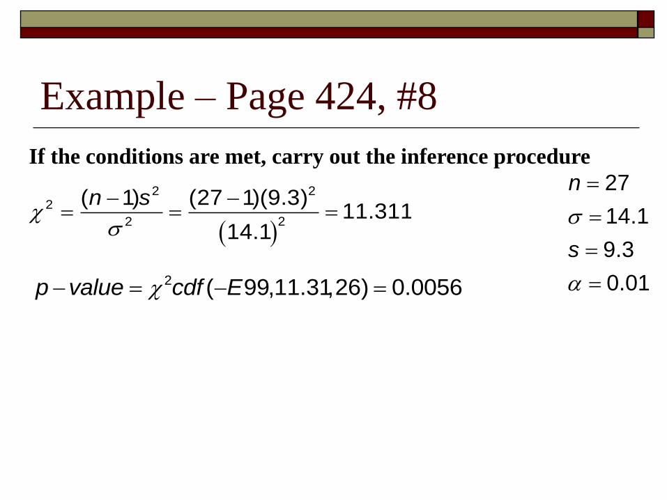
Example – Page 424, #8
27
14.1
9.3
0.01
n
s
2 ( 99,11.31,26) 0.0056p value cdf E
2 22
22
( 1) (27 1)(9.3)11.311
14.1
n s
If the conditions are met, carry out the inference procedure

Example – Page 424, #8
Reject Ho since P-value ≥ α, there and conclude that the standard
deviation of test scores is less than 14.1.
No, a lower standard deviation does not suggest that the current
class is doing better, but they are more similar to each other and
show less variation. Standard deviation speaks only about the
spread of the scores not their location.
Interpret your results in the context of the problem